mode i fracture criterion and the finite...
TRANSCRIPT

MODE I FRACTURE CRITERION AND THE FINITE-WIDTH CORRECTION FACTOR FOR NOTCHED LAMINATED COMPOSITES
By
BOKWON LEE
A THESIS PRESENTED TO THE GRADUATE SCHOOL OF THE UNIVERSITY OF FLORIDA IN PARTIAL FULFILLMENT
OF THE REQUIREMENTS FOR THE DEGREE OF MASTER OF SCIENCE
UNIVERSITY OF FLORIDA
2003

Copyright 2003
by
Bokwon Lee

To my parents, Jonghan Lee and Jongok Woo
iv
ACKNOWLEDGMENTS
I am grateful to Dr. Bhavani V. Sankar for giving me the opportunity of pursuing this
research and for the insightful guidance he provided me, not only in the research work, but
throughout the course of my graduate studies at the University of Florida. I would also like to
express my gratitude to Dr. Peter G. Ifju and Dr. Ashok V. Kumar for serving as my
supervisory committee members and for giving me advice.
I must also acknowledge the Korea Airforce for giving me an opportunity to study
abroad and meet wonderful people in the research world. The experience I have gained at the
Center for Advanced Composites will be greatly helpful to me in my duties as an Airforce
Logistics Officer.
I wish to thank all my fellow students for the fun and support. I greatly look forward to
having all of them as colleagues in the years ahead.
The final acknowledgement goes to all of my family, Jonghan Lee, Jongok Woo, and
Hongwon Lee, for their unconditional support and love.

v
TABLE OF CONTENTS
page
ACKNOWLEDGMENTS ...................................................................................................iv LIST OF TABLES .............................................................................................................. vii LIST OF FIGURES ........................................................................................................... viii ABSTRACT.........................................................................................................................xi CHAPTERS
1 INTRODUCTION........................................................................................................... 1 1.1 Background and Objectives ........................................................................................ 1 1.2 Literature Review........................................................................................................ 3
2 LAY-UP INDEPENDENT FRACTURE CRITERION.................................................... 7
2.1 Introduction................................................................................................................ 7 2.2 Stress Intensity Factor Measurements.......................................................................... 8 2.2.1 Experimental Background.................................................................................. 8 2.2.2 Stress Intensity Factor Calculations.................................................................. 10 2.3 Derivation of Stress Intensity Factor in the Load-Carrying Ply.................................... 12 2.4 Results and Discussion.............................................................................................. 15
3 FINITE ELEMENT ANALYSIS ................................................................................... 18
3.1 2D Finite Element Global Model................................................................................ 18 3.2 2D Finite Element Sub-Model................................................................................... 26 3.3 Comparison and FE Results and Analytical Model..................................................... 31 3.4 Finite-Width Correction Factor ................................................................................. 34 3.4.1 Isotropic Finite-Width Correction Factor......................................................... 34 3.4.2 Orthotropic Finite-Width Correction Factor..................................................... 35 3.4.2.1 Developing procedure for FWC solution............................................. 35 3.4.2.2 Anisotropy parameter, ..................................................................... 42

vi
3.5 Effect of Blunt Crack Tip........................................................................................... 43 3.5.1 2D FE Modeling Procedure ............................................................................ 43 3.5.2 Results and Discussion.................................................................................... 44 3.6 Effect of Local Damage............................................................................................. 46 3.6.1 3D FE Modeling Procedure for Delamination................................................... 49 3.6.2 3D FE Modeling Procedure for Axial Splitting ................................................. 51 3.6.3 Results and Discussion.................................................................................... 52 3.7 Summary of FE Results and Discussion...................................................................... 53
4 CONCLUSIONS AND FUTURE WORK.................................................................... 55
4.1 Conclusions .............................................................................................................. 55 4.2 Future Work............................................................................................................. 59
APPENDIX A LAMINATION THEORY ............................................................................................ 60 B MATHEMATICAL THEORY OF BRITTLE FRACTURE........................................... 63 LIST OF REFERENCES ................................................................................................... 67 BIOGRAPHICAL SKETCH.............................................................................................. 69
vii
LIST OF TABLES
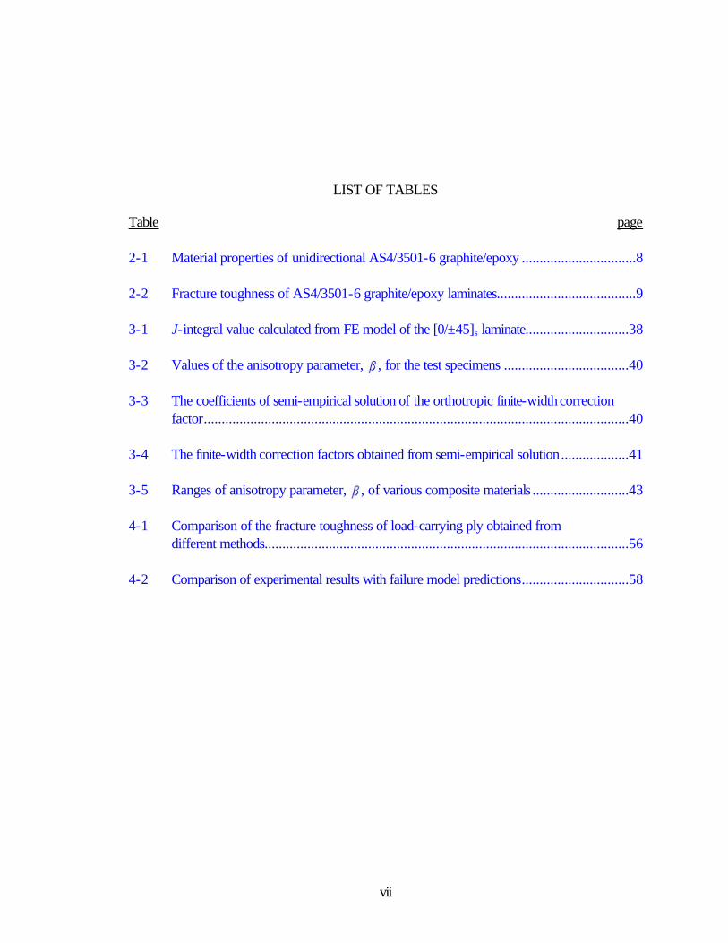
Table page 2-1 Material properties of unidirectional AS4/3501-6 graphite/epoxy ................................8 2-2 Fracture toughness of AS4/3501-6 graphite/epoxy laminates.......................................9 3-1 J-integral value calculated from FE model of the [0/±45]s laminate.............................38 3-2 Values of the anisotropy parameter, , for the test specimens ...................................40 3-3 The coefficients of semi-empirical solution of the orthotropic finite-width correction
factor.......................................................................................................................40 3-4 The finite-width correction factors obtained from semi-empirical solution...................41 3-5 Ranges of anisotropy parameter, , of various composite materials ...........................43 4-1 Comparison of the fracture toughness of load-carrying ply obtained from different methods......................................................................................................56 4-2 Comparison of experimental results with failure model predictions..............................58

viii
LIST OF FIGURES
Figure page 2-1 Specimen specification and fiber directions..................................................................8 2-2 Local coordinate system of crack tip area stress components ....................................12 2-3 Comparison of the fracture toughness of the load-carrying ply ...................................15 3-1 Scheme of two-dimensional FE model of [0/±45]s laminate.......................................20 3-2 Finite element global model mesh and boundary condition.........................................21 3-3 Scheme of 2D FE global model analysis procedure ...................................................22 3-4 Normal stress distribution in the global model in the [0/±45]s laminate........................24 3-5 Stress intensity factor in the global model in the [0/±45]s laminate ..............................24 3-6 distribution in the [0/±45]s laminate under a load of 351.14 MPa .........................25 3-7 Different sizes of sub-model......................................................................................27 3-8 Comparison of SIF obtained from different sizes of sub-model..................................27 3-9 Finite element sub-model mesh and linking with global model.....................................28 3-10 Normal stress distribution in the sub-model in case of [0/±45]s laminate.....................29 3-11 Stress intensity factor in the sub-model in case of [0/±45]s laminate ...........................29 3-12 distribution in the [0/±45]s laminate under a load of 351.14 MPa..........................30 3-13 Comparison of normal stress distribution in the sub-model and global model in
case of [0/±45]s laminate..........................................................................................32 3-14 Stress intensity factor in the global model in case of [0/±45]s laminate........................32

ix
3-15 Stress intensity factor in the sub-model in case of [0/±45]s laminate ...........................33
3-16 Comparison of the fracture toughness of principal load-carrying ply...........................33 3-17 Comparison of the finite-width correction factors in an isotropic plate computed by the
finite element methods with the closed form solution..................................................37 3-18 J-integral vs. contour line calculated from FE model of the [0/±45]s laminate..............38 3-19 The finite-width correction factors vs. ratio of crack size to panel width.....................39 3-20 The finite-width correction factors vs. anisotropy parameter ......................................39 3-21 The finite-width correction factors as a function of anisotropy parameter, ,and
ratio of crack size to panel width, a/w ......................................................................41 3-22 Anisotropy parameter, , as a function of lamination angle for graphite/epoxy [± ]s
and [0/± ]s laminates...............................................................................................42 3-23 Crack tip shape profiles............................................................................................44 3-24 Effect of crack tip shape on predicted fracture toughness of [0/±45]s laminate ; 2D
FE global model results ............................................................................................45 3-25 Effect of crack tip shape on predicted fracture toughness of [0/±45]s laminate ; 2D
FE sub-model results................................................................................................45 3-26 Von-Mises stress distribution in [0/±45]s laminate.....................................................48 3-27 Comparison of stress intensity factor of the load-carrying ply between 2D and 3D
global model............................................................................................................49 3-28 Scheme of ply interface mesh in the [0/±45]s laminate................................................50 3-29 Estimated delamination area on interface between 0E and +45E ply in the [0/±45]s
laminate ...................................................................................................................50 3-30 Axial splitting failure mode in the load-carrying ply.....................................................51 3-31 Estimated axial splitting area on interface between 0E and +45E ply...........................52 3-32 Effect of the local damage on normal stress distribution in the load-carrying ply in
the [0/±45]s laminate................................................................................................53

x
3-33 Effect of the local damage on stress intensity factor in the load-carrying ply................54 4-1 Comparison of the fracture toughness of the load-carrying ply ...................................56 4-2 Comparison of experimental results with failure model predictions..............................57 4-3 Comparison of experimental results with failure model predictions (log scale) .............58 A-1 Laminated plate geometry.........................................................................................61 B-1 Stress components in the vicinity of crack tip.............................................................65

xi
Abstract of Thesis Presented to the Graduate School of the University of Florida in Partial Fulfillment of the Requirements for the Degree of Master of Science
MODE I FRACTURE CRITERION AND THE FINITE-WIDTH CORRECTION FACTOR FOR NOTCHED LAMINATED COMPOSITES
By
Bokwon Lee
August 2003
Chair: Bhavani V. Sankar Major Department: Mechanical and Aerospace Engineering
The purpose of this study was to investigate the applicability of the existing lay-up
independent fracture criterion for notched composite laminates. A detailed finite element analysis
of notched graphite/epoxy laminates was performed to understand the nature of stresses and
crack tip parameters in finite-width composite panels. A new laminate parameter β has been
identified which plays a crucial role in the fracture of laminated composites. An empirical
formula has been developed for finite-width correction factors for composite laminates in terms
of crack length to panel width ratio and β . The effects of blunt crack tip and local damage on
fracture behavior of notched composite laminates are investigated using the FE analysis. The
results of experiments performed elsewhere are analyzed in the light of new understanding of
crack tip stresses, and the applicability of the lay-up independent fracture criterion for notched
composite laminates is discussed. It is determined that the analytical lay-up independent fracture

xii
model that considers local damage effect provides good correlation with experimental data, and
the use of orthotropic finite-width correction factor improves the accuracy of notched strength
prediction of composite laminates.

1
CHAPTER 1 INTRODUCTION
1.1 Background and Objectives
Composite laminates are widely used in aerospace, automobile and marine
industries. Because of their high strength-to-weight and stiffness-to-weight ratio, use of
fiber-reinforced composite materials in advanced engineering structures such as high-
performance aircraft has been increasing. Recently, laminated composites have been
increasingly used in military fighter airframes and external surfaces because those
designs are required to handle high aerodynamic forces, be lightweight for maximizing
air-to-air performance, minimize radar cross section, and withstand foreign object and
battle damage. In addition, by properly sequencing the stacking lay-up, a wide range of
design requirements can be met. Laminated composites posses distinctive advantages as
mentioned above; however, fiber-reinforced composites exhibit notch sensitivity, and this
can be an important factor in determining safe design. The problem of predicting the
notched strength of laminated composites has been the subject of extensive research in
the past few years. Owing to the inherent complexity and the number of factors involved
in their fracture behavior, several semi-empirical failure criteria have been proposed and
have gained popularity. Some failure criteria are based on concepts of linear-elastic
fracture mechanics (LEFM), while others are based on the characteristic length and stress
distribution in the vicinity of the notch. In general, these models rely on a curve-fitting
procedure for the determination of a number of material and laminate parameters,
involving testing of notched and unnotched specimens for each selected lay-up.

2
One limitation commonly reported is that the fracture toughness in many cases is
dependent upon laminate configuration, the specific fiber/matrix system, etc. The use of
these failure criteria without properly accounting for this dependence has led to some
mixed results. Awerbuch and Madhukar [1] reviewed some of the most commonly used
fracture criteria for notched laminated composites. They collected data from several
sources and different materials and evaluated the performance of each criterion. They
concluded that the parameters are strongly dependent on laminate configuration and
material system and must be determined experimentally for each new material system
and laminate configuration. To overcome this limitation of those popular failure criteria,
recently a lay-up independent fracture criterion was developed by employing linear-
elastic fracture mechanics concepts. The fracture toughness of the load-carrying ply in
the presence of fiber breakage was considered as the principal fracture parameter.
The main objective of this research was to further verify and also improve the
existing lay-up independent fracture criterion for notched laminated composites. Detailed
finite element analyses, both 2D and 3D, of the laminate were performed to understand
the average laminate stresses as well as stresses in individual layers. An analytical model
for determining the principal fracture parameter, fracture toughness of the load-carrying
ply, was also developed. It has been found that factors such as crack bluntness, local
damage such as fiber splitting, delamination, etc. in the vicinity of crack tip play a
significant role in reducing the stresses in angle plies and thus increasing the stresses and
stress intensity factor in the load-carrying ply. A new laminate parameter, referred to as
β , has been identified. This parameter represents the ratio of the axial and normal
stresses at points straight ahead of crack tip, and plays a crucial role in the failure of the

3
notched laminate.
A secondary objective was to develop a semi-empirical solution for finite-width
correction factor (FWC) for laminated composites to improve the accuracy of prediction
of notched strength. Due to the lack of a closed form solution for orthotropic finite-width
correction factor, most existing failure criterion used the isotropic finite-width correction
factor for prediction of notched strength of laminates. In some cases, the application of
the isotropic finite-width correction factors to estimate the anisotropic or orthotropic
finite-width correction factors can cause significant error. An attempt was made to
reduce the error in predicting the notched strength by developing an orthotropic finite-
width correction factor for various laminates configurations.
1.2 Literature Review
Numerous failure models have been developed for the prediction of the notched
strengths of composite laminates. Due to the complication of analyzing the fracture
behavior of notched composite laminates, a number of assumptions and approximations
were contained in most commonly used failure models to predict the tensile strengths of
notched composite laminates. In recent years several simplified fracture models have
been proposed. The scope of this research was limited to laminated composites
containing a straight center crack when subjected to uniaxial tensile loading.
Waddoups, Eisenmann, and Kaminkski (WEK-LEFM models) [2] applied Linear
Elastic Fracture Mechanics to composites. Their approach was to treat the local damage
zone as a crack, and apply fracture mechanics. Whitney and Nuismer [3] proposed the
stress-failure models. These models named the Average-Stress Criterion (ASC) and the
Point-Stress Criterion (PSC) assumed that fracture occurs when the point stress or the
4
average stress over some characteristic distance away from the discontinuity is equal to
the ultimate strength of the unnotched laminate. The characteristic distances in point
stress criterion and average-stress criterion, are considered to be material constants and
the evaluation of the notched tensile strength is based on the closed form expressions of
the stress distribution adjacent to the circular hole. Tan [4] extended this concept and
developed more general failure models, the Point Strength Model (PSM) and Minimum
Strength Model (MSM). These models successfully used to predict the notched strength
of composite laminates subjected to various loading conditions. Such models using a
characteristic length concept have been widely used to predict ultimate strength in the
presence of notches. The main disadvantage is that the characteristic length is not a
material constant and depends on factors such as the lay-up configuration, the geometry
of the notch, etc. Therefore, the characteristic length obtained from tests on one laminate
configuration may not be extrapolated to predict the failure of other laminates of the same
material system. Mar and Lin [5] proposed LEFM fracture model called Mar-Lin
criterion, the damage zone model, and the damage zone criterion. They assumed that the
laminate fracture must occur through the propagation of a crack lying in matrix material
at the matrix/filament interface. It was able to provide good correlation with experimental
data and at the same time is very simple to apply. However, the fracture parameter, which
was used in Mar-Lin criterion, depends on the laminate lay-up configuration. Therefore,
the application of this fracture criterion requires experimental determination of the
fracture parameter for each laminate. Chang and Chang [6] and Tan [7] proposed
progressive damage models which were developed to predict the extent of damage and
damage progression, respectively, in notched composite laminates. The models accounted

5
for the reduced stress concentration associated with mechanisms of damage growth at a
notch tip by reducing local laminate stiffness.
Past experimental investigations, which were carried out by Poe [8], have
revealed that fiber failure in the principal load-carrying plies governs the failure of
notched laminated composites. Poe and Sova [8, 9] proposed a general fracture-
toughness parameter, critical strain intensity factor, which is independent of laminate
orientation. This parameter was derived on the basis of fiber failure of the principal load-
carrying ply and it is proportional to the critical stress intensity factor. Such an idea was
adopted by Kageyama [10] who estimated the fracture toughness of the load-carrying ply
by three dimensional finite element analysis. Such analyses led to lay-up independent
fracture criteria based on the failure mechanism of the load-carrying ply, which governs
the failure of entire laminate. Recently, Sun et al. [11, 12] proposed a new lay-up
independent fracture criterion for composites containing center cracks. In their analysis,
the fracture toughness of the load-carrying ply was introduced as the material parameter.
Such an analysis is approximate, since it does not take into account any stress
redistribution caused by local damage and it used the isotropic form factor instead of an
orthotropic finite-width correction factor to account for finite width of the laminated
specimens.
There are several analytical and numerical methods [13-15] to determine the
orthotropic finite-width correction factor including the boundary integral equation, finite
element analysis, modification of isotropic finite-width correction factor, etc. However,
no closed form solutions are available. Therefore, the closed form solution for isotropic
materials is frequently used for orthotropic material as well.

6
Current study aims to further verify the lay-up independent model including new
fracture parameter and improve the accuracy for the notched strength prediction of
composite laminates by using orthotropic finite-width correction factor.
Chapter 1 provides an introduction and a literature review of fracture models for
notched laminated composites. Chapter 2 describes a general concept of the lay-up
independent fracture model and the analytical derivation of the stress intensity factor in
the load-carrying ply. Chapter 3 describes a FE modeling procedure including damage
modeling and the development of the orthotropic finite-width correction factor based on
FE analysis. Conclusions and some recommendations for future work are presented in
Chapter 4.

7
CHAPTER 2 LAY-UP INDEPENDENT FRACTURE CRITERION
2.1 Introduction
Fibrous composite materials have high strength and stiffness as mentioned before.
Under tension loading, however, most advanced laminated composites are severely
weakened by notches or by fiber damage. Thus, a designer needs to know the fracture
toughness of composite laminates in order to design damage tolerant structures. The
fracture toughness of composite laminates depends on material property and laminates
configuration. Consequently, testing to determine fracture toughness for each possible
laminate configuration would be expensive and time-consuming work. Thus, a single
fracture parameter can be used to predict fracture toughness for all laminates
configurations of the same material system. Poe and Sova [8, 9] proposed a general
fracture toughness parameter, CQ , which was derived using a strain failure criterion for
fibers in the load-carrying ply. Sun and Vaiday [11] also proposed a single fracture
parameter, stress intensity factor in the load-carrying ply which was derived using
classical lamination theory and LEFM theory.
In this chapter, exact LEFM analytical expression for lay-up independent failure
model is presented and it is compared with the similar methodology proposed by Sun and
Vaiday [11]

8
2.2 Stress Intensity Factor Measurements
2.2.1 Experimental Background
As mentioned earlier we have analyzed the results of fracture tests performed by
Sun et al. [11, 12]. The material properties, laminate configurations used and failure load
are presented here for the sake of completion. Nine different laminate configurations
made from AS4/3501-6 (Hercules) graphite/epoxy were tested. The panels were made of
unidirectional prepreg tape with a nominal thickness of 0.127 mm. The material
properties for this unidirectional prepreg tape are shown in Table 2-1. The panel
specifications, geometry, and coordinate system used for the present analysis is shown in
Figure 2-1. All the test specimens reported here were fabricated using the hand lay-up
technique and cured in an autoclave. Different laminate configurations were selected such
that each one had at least one principal load-carrying ply (0E), i.e., plies with fibers
aligned along the loading direction.
Table 2-1 Material properties of unidirectional AS4/3501-6 graphite/epoxy
Young’s Moduli (GPa) Poisson’s Ratio
Shear modulus Material
EL ET vLT GLT, (GPa)
Prepreg thickness
(mm) graphite/epoxy 138 9.65 0.3 5.24 0.127
Figure 2-1 Specimen specification and fiber directions

9
To make the crack, a starter hole was first drilled in the laminates to minimize any
delamination caused by the waterjet. The crack was then made by a waterjet cut and
further extended with a 0.2 mm thick jeweler’s saw blade.
The failure stress (load over nominal cross section of the laminate) for each
laminate configuration tested are shown in Table 2-2. The fracture toughness estimated
using the nominal stress intensity factor for the laminate is shown under the column
“Laminate fracture toughness”. This is computed using the formula
awaYK yQ πσ )/(∞= (1)
where ∞yσ is the remote stress and Y is the finite-width correction factor. Sun et al. [11, 12]
used the Y for isotropic material which is equal to 1.0414 for the present case
(a/w=0.2627). One can note that the fracture toughness estimated using this method is not
the same for different laminates and hence cannot be considered as a material property.
The last column of Table 2-2 is the fracture toughness of the load-carrying ply calculated
by Sun and Vaiday [11], which will be discussed in subsequent sections.
Table 2-2 Fracture toughness of AS4/3501-6 graphite epoxy laminates [11]
Notation Laminate configuration
Failure stress (MPa)
Laminate fracture toughness QK ( )mMPa
Fracture toughness of the load-carrying ply
LQK ( )mMPa
S1 [0/90/±45]s 343.00 44.83 ± 3.05 115.66
S2 [±45/90/0]s 323.27 42.19 ± 1.87 108.82
S3 [90/0/±45]s 316.05 41.25 ± 1.46 106.43 S4 [0/±15]s 695.84 90.82 ± 4.01 101.81 S5 [0/±30]s 466.14 60.84 ± 3.14 101.00 S6 [0/±45]s 351.14 45.83 ± 2.17 106.32 S7 [0/90]2s 446.76 58.31 ± 5.30 109.04
S8 [±45/0/±45]s 287.16 37.48 ± 0.43 119.81 S9 [±452/0/±45]s 248.40 32.42 ± 0.60 123.64

10
2.2.2 Stress Intensity Factor Calculations
A parameter commonly used to represent the notch sensitivity of materials is the
critical stress intensity factor (S.I.F.) or the fracture toughness, QK . Numerous
investigations have attempted to determine the critical stress intensity factor for a variety
of composite laminates, and those results indicate that it depends primarily on the
material, laminate configuration, stacking sequence, specimen geometry and dimensions,
notch length, etc. In addition, stress intensity factor is strongly affected by the extent of
damage and failure modes at the notch tip. Therefore, it is a critical parameter to design
composite laminates structure.
The stress intensity factor of notched laminates can be calculated in three
different ways.
1. From Eq. (1) using failure stress directly from the experiment
2. Finite Element Analysis I : From the normal stress distribution obtained from a
series of finite element models using the following equation.
rrK yrI πσ 2)0,(lim0→
= (2)
where r is the distance from the crack tip and normal stress component yσ (r,0) is the
average stress of the each ply.
3. Finite Element Analysis II : From the J- integral calculated from finite element
models. The relation of the energy release rate and stress intensity factor is given by the
following equation [17].
2/1
11
6612
2/1
11
222/1
22112
22
2
++
=
aaa
aaaa
KG II (3)

11
where ija are elastic constants. When the remote applied stress is the failure stress, stress
intensity factor IK becomes the fracture toughness QK . The stress intensity factor of the
load-carrying ply, LQK , can be estimated in two different ways.
1. From simple stress analysis using LEFM and lamination theory by calculating
the portion of the applied load that is carried by the load-carrying ply. The analytical
derivation of the fracture toughness of the load-carrying ply is presented in following
section.
2. Same procedure as in Eq. (2) but using normal stress field of the load-carrying
ply extracted from a series of finite element models using the following equation.
rrK Lyr
LI πσ 2)0,(lim
0→= (4)
In order to estimate fracture toughness of various laminates configurations, the
failure stresses of the notched laminates have to be determined from experiments.
However, if the general fracture parameter, the fracture toughness of the load-carrying
ply which is lay-up independent, is determined from preliminary test, laminates fracture
toughness can be obtained using simple analysis. Consequently, it will be discussed in the
following section.
2.3 Derivation of Stress Intensity Factor in the Load-Carrying Ply
In this section, we derive an analytical expression for the stress intensity factor for
the load-carrying ply in terms of the average laminate stress intensity factor obtained
using three methods mentioned earlier. The derivation of stress intensity factor presented
here is based on LEFM and classical lamination theory. The detailed derivation
procedure can be found in Appendix A and B.

12
Figure 2-2 Local coordinate system of crack tip area stress components
The state of stress in the vicinity of a crack in an orthotropic material is given by
[ ]1Re2
)0,(r
Kr I
y πσ = (5.a)
( ) [ ]21Re2
0, ssr
Kr I
x −=π
σ (5.b)
where the parameters s1 and s2 are related to the orthotropic elastic constants as explained
in Appendix B. We will use a new laminate parameter β to denote the ratio between the
two normal stresses shown in Eqs. (5.a) and (5.b).
( )( ) [ ]21Re
0,0, ss
rr
y
x −==σσβ (6)
We will use the classical lamination theory to extract the stresses in the load-carrying ply
from the force resultants acting in the entire laminate. According to the classical
lamination theory presented in Appendix A, in the case of symmetric laminated plates
without coupling under plane stress or plane strain conditions, the force-mid-plane strain
equations can be expressed in matrix form as

13
=
0
0
0
662616
262212
161211
xy
y
x
zy
y
x
AAAAAAAAA
NNN
γεε
(7)
where [A] is the laminate extensional stiffness matrix. The inverse relation is given by
=
xy
y
x
xy
y
x
N
NN
AAA
AAAAAA
*66
*26
*16
*26
*22
*12
*16
*12
*11
0
0
0
γεε
(8)
where superscript * denotes the component of inverse matrix of [ ]A . The stresses in the
load-carrying ply can be derived from the mid-plane strains as
=
0
0
0
662616
262212
161211
xy
y
x
LLL
LLL
LLL
Lxy
Ly
Lx
QQQ
QQQ
QQQ
γεε
τσσ
(9)
where superscript L indicates the load carrying ply and the quantities Qij (i,j = 1, 2, 6) are
the stiffness coefficients of the principal load carrying plies. Substituting Eq. (8) into Eq.
(9) yields the following equation.
=
xy
y
x
LLL
LLL
LLL
Lxy
Ly
Lx
NNN
AAAAAAAAA
QQQ
QQQ
QQQ
*66
*26
*16
*26
*22
*12
*16
*12
*11
662616
262212
161211
τσσ
(10)
In the vicinity of the crack tip the force resultants can be written in terms of the average
stresses in the orthotropic laminate
0,, ===== xyxyyyyxx tNtNttN τσβσσ (11)

14
where t is the total thickness of laminates. Substituting from Eq. (11) into Eq. (10) we
obtain the stresses in the load-carrying ply as
( )yLLL
LLL
LLL
Lxy
Ly
Lx
tAAAA
AA
QQQ
QQQ
QQQ
σβββ
τσσ
+++
=
*26
*16
*22
*12
*12
*11
662616
262212
161211
(12)
In particular we are interested in the stress component Lyσ responsible for fracture and it
is obtained from Eq. (9) as
( ) ( )[ ] ( )y
LLLy tAAQAAQ σββσ *
22*1222
*12
*1112 +++= (13)
Then the stress intensity factor LQK in the load-carrying ply can be expressed in terms of
the laminate stress intensity factor QK as
( ) ( )[ ] Q
LLLAQ KAAQAAQtK *
22*1222
*12
*1112)( +++= ββ (14)
In deriving Eq. (14) we have used the assumption QLQy
Ly KK // =σσ .
The lay-up independent fracture criteria assume that there is a critical value of
LQK for each material system and is independent of laminate configuration as long as
there is a load-carrying ply in the laminate. In order to verify this concept we computed
QK from the experimental failure loads [11] using Eq. (1). Then LQK at the instant of
fracture initiation was computed using Eq. (14). The resulting fracture toughness will be
called LAQK )( .
Sun and Vaiday [11] used a similar approach to calculate the stress intensity
factor in the load-carrying ply, but they used the remote stresses applied to the laminate

15
in order to determine the ratio of yx σσ / . Since the applied load is uniaxial, this ratio
was equal to zero in their case. This is equivalent to taking the factor β as equal to zero.
It should be emphasized that this stress ratio is not equal to zero in the vicinity of the
crack tip, as there is a nonzero component of xσ is present (see Eq. 5b). We denote this
fracture toughness as LBQK )( . Thus the relation between L
BQK )( and QK can be obtained by
setting β =0 in Eq. (14) and it takes the form
[ ] Q
LLLBQ KAQAQtK *
2222*1212)( += (15)
2.4 Results and Discussion
The values of LAQK )( and L
BQK )( are shown in Figure 2-3 for the nine laminate
configurations. The average values and corresponding standard deviation are 74.35 MPa-
m1/2 and 18.35 % for LAQK )( , and 110.28 MPa-m1/2 and 9.8 % for L
BQK )( . Surprisingly the
case B wherein the β value was taken as zero yielded consistent layer independent
fracture toughness compared to the case A where the actual stress ratio (β>0) was used.
0
20
40
60
80
100
120
140
S1 S2 S3 S4 S5 S6 S7 S8 S9
Figure 2-3 Comparison of the fracture toughness of the load-carrying ply
Laminate configuration
LBQK )(
LAQK )(
F
ract
ure
toug
hnes
s,
(MP
a-m
1/2
)
16
Such analyses are approximate, since they do not consider any stress
redistribution caused by physical fracture behavior such as local damage in the form of
matrix cracking, delamination, etc. In order to fully understand the nature of crack tip
stress field in finite-width laminates a detailed finite element analysis was performed.
The procedures and the results are discussed in Chapter 3.

17
CHAPTER 3 FINITE ELEMENT ANALYSIS
A detailed finite element analysis of fracture behavior of notched laminated
composites was conducted in conjunction with the analytical failure models described
earlier. The purpose of the finite element analysis was to develop a model that could
predict the fracture parameters of notched laminated composites and investigate the effect
of local damage and crack tip shape on the stress intensity factor for notched laminated
composites. Another goal of the study was to determine the orthotropic finite-width
correction factor using J- integral. One of the leading commercial FE packages, ABAQUS
6.2 [18] was used to analyze the various test specimens. Two types of analyses were
performed. In the 2D model the specimens were modeled as orthotropic laminate. In the
second model 3D solid elements were used to model the individual layers of the laminate.
In both cases sub-modeling was performed to improve the accuracy of the calculated
crack tip parameters such as stress intensity factor and J-Integral. The mode I stress
intensity factor, IK , can be calculated in two different ways based on the finite element
analysis as mentioned earlier.
However, stress intensity factor of the load-carrying ply can be calculated only
one way using the Eq. (4) because ABAQUS can not calculate J-integral for each ply
level. )0,(rLyσ is extracted from normal stress field in the load-carrying ply of FE model.
The stress intensity factors obtained using the above methods from two types of
FE models are compared with the analytical models in the subsequent section.

18
It is noted that overall analysis procedure and detailed results are presented for
case of the [0/±45]s laminate and the results of other eight laminate configurations are
summarized.
3.1 2D Finite Element Global Model
The purpose of the 2D analysis is to compare the results with the analytical model
so that the effect of finite-width of the specimen can be understood. Further FE models
can be used to understand the effects of blunt crack tip and also other forms of damage
such as delamination and fiber splitting. The various laminate configurations with center
notch were modeled with eight node plane stress elements (CPS8R element). A quarter
model was used, with symmetric boundary conditions. The width of the model, w, was
19.05 mm, and the length was 254 mm. The notch was modeled as a sharp crack with a
half width, a= 5 mm. Since the lay-up is symmetric, it was only necessary to model half
of the thickness.
The main difference between global model and sub-model is mesh refinement.
The FE global model uses relatively coarse mesh compared to the FE sub models. A
fixed element size with width of 1 mm was used in the FE global model. A relatively fine
mesh was used adjacent to the notch. The geometry and the finite element models were
created using ABAQUS/CAE modeling tool and ABAQUS keyword editor. Figure 3-2
shows the initial mesh of the upper left quadrant. Separate elements were used to
represent each ply and common nodes were used for interface of plies. Figure 3-1 shows
the scheme of two-dimensional FE model of [0/±45]s laminate. Figure 3-3 shows the
overall global modeling procedure in case of [0/±45]s laminate. The material property of
each ply was modeled as a homogeneous linear elastic orthotropic material throughout

19
this FE analysis. In order to use a single global coordinate system, the material properties
of angle plies were transformed using the transformation relation for engineering
constants. Orthotropic properties for AS4/3501-6 graphite/epoxy unidirectional prepreg
were defined as shown in Table 2-1. The material property of each angle ply was
implemented in ABAQUS by means of user material subroutine (UMAT). The fixed grip
loading condition was simulated by constraining the nodes along the edge of the plate to
have the same displacement under an applied load. This was also implemented by using
the EQUATION command. The failure load obtained from experiments (see Table 2-1)
was applied. In global model analysis, J- integral also was calculated using ten contour
lines to determine the orthotropic finite-width correction factors. It will be discussed in
Chapter 3.4.

20
Figure 3-1 Scheme of two-dimensional FE model of [0/±45]s laminate

21
Figure 3-2 Finite element global model mesh and boundary condition

22
Figure 3-3 Scheme of 2D FE global model analysis procedure
FE commercial package ABAQUS 6.2
PRE-PROCESSING
ANALYSIS: ABAQUS/Strandard
POST-PROCESSING: ABAQUS/Viewer
ABAQUS/CAE Keyword Editor
User Material Subroutine
G_S42D.inp : modeling input data G_S42D.fil : results for interpolation to sub-model boundary G_S42D.dat : numerical data of FE analysis G_S42D.odb : visualization data
Microsoft EXCEL
MATLAB � Convert J-integral to K using Eq. 3
G_S42D.cae/msg/res/com/...etc
� Transform material property of 0E ply to angle ply
� Geometry modeling * elcopy, element shift=10000, shift nodes=0 : duplicate element to model
each ply and common nodes are used for interface of each ply
Par
t/Ass
embl
y
� Material property modeling for each ply : User material subroutine M
ater
ial
� Boundary and load condition * Equation : define grip condition : define symmetric boundary condition Lo
ad
� History output and field output request * contour integral, contours=10,symm : stress, displacement, contour integral, ,crack,1.0,0.0 : request J-intergral UVAR and define crack tip normal vector * node file, U,S : request data for
interpolation to submodel boudnary St
ep
� Mesh modeling and Element definition : CPS8R element M
esh
Sub-model Analysis
� Visualize the stress and displacement distribution
� Calculate K using Eqs. 2, 4
� Request to generate G_S42D.inp � Submit input file to ABAQUS/standard Jo
b
User Variable Subroutine � Define a user variable

23
Figure 3-4 shows the distribution of normal stress of the load-carrying ply and
average normal stress of the laminate, respectively, for the global model. From the
normal stress distribution in the Figure 3-4, it is clear that yσ stress in the load-carrying
ply is much higher than the average and hence that of angle ply. In the Figure, yσ was
defined as 3
4545 −+ ++ yyLy σσσ
. A contour plot of yσ distribution is shown in Figure 3-6.
Figure 3-5 shows the values of rLy πσ 2 and ry πσ 2 as a function of r in the [0/±45]s
laminate. The stress intensity factor of the load-carrying ply and the laminate can be
obtained by extrapolating measured normal stress distribution from the FE global model
based on Eqs. (2) and (4). The stress intensity factor obtained from global FE model
agree well with the analytical model case B (Eq. 15) which was calculated assuming xσ =
0 ahead of crack tip.

24
0.00E+00
1.00E+09
2.00E+09
3.00E+09
4.00E+09
5.00E+09
6.00E+09
0.00E+00 2.00E-03 4.00E-03 6.00E-03 8.00E-03 1.00E-02 1.20E-02 1.40E-02
Figure 3-4 Normal stress distribution in the global model in the [0/±45]s laminate
0.00E+00
5.00E+07
1.00E+08
1.50E+08
2.00E+08
2.50E+08
3.00E+08
0.00E+00 2.00E-03 4.00E-03 6.00E-03 8.00E-03 1.00E-02 1.20E-02 1.40E-02
Figure 3-5 Stress intensity factor in the global model for [0/±45]s laminate
Distance from crack tip, r (m)
N
orm
al s
tres
s, (
MP
a)
Lyσ in the load-carrying ply Lxσ in the load-carrying ply
yσ in the laminate
xσ in the laminate
Distance from crack tip, r (m)
S
tres
s In
tens
ity fa
ctor
,
(MP
a-m
1/2
)
rLy πσ 2 in the load-carrying ply
ry πσ 2 in the laminate
Extrapolation line y = 1.17E+10x + 1.07E+08
Extrapolation line y = 4.88E+09x + 4.59E+07

25
(a) Load-carrying ply, 0Edegree
(b) +45E ply
Figure 3-6 yσ distribution in the [0/±45]s laminate under a load of 351.14 MPa

26
3.2 2D Finite Element Sub-Model
The analysis was repeated with a very refined element size in order to investigate
the local fracture behavior and the sensitivity of the results to mesh refinement. All other
aspects of the analysis were kept the same as global model. For efficiency of
computation, the finite element sub-modeling analysis technique was adopted. The sub-
modeling analysis is most useful when it is necessary to obtain an accurate, detailed
solut ion in a local area region based on interpolation of the solution from an initial,
relatively coarse, global model. The sub-model is run as a separate analysis. The link
between the sub-model and the global model is the transfer of results saved in the global
model to the relevant boundary nodes of the sub-model. Thus, the response at the
boundary of the sub-model is defined by the solution of the global model. However, in
order to adopt sub-modeling technique, the accuracy of sub-model should be ensured by
checking the comparing important parameter to determine reasonable sub-modeling size.
Three different sizes of sub-models were modeled to determine adequate sub-model size
to minimize the execution time and maximize accuracy. Figure 3-7 shows the different
size of sub-model and Figure 3-8 shows the results of comparison of stress intensity
factor obtained from sub-models with stress intensity factor obtained from J- integral
using Eq. (3). For efficiency of computation, sub-model size B was chosen for
subsequent studies.

27
Figure 3-7 Different sizes of sub-model (A= 10 %, B= 20 %, C= 40 % of crack size, a)
Figure 3-8 Comparison of SIF obtained from different sizes of sub-model
0
10
20
30
40
50
60SIF obtained from J-integral in the global model
A B C
S
tres
s In
tens
ity fa
ctor
,
(MP
a-m
1/2
)
sub-model A sub-model B sub-model C
28
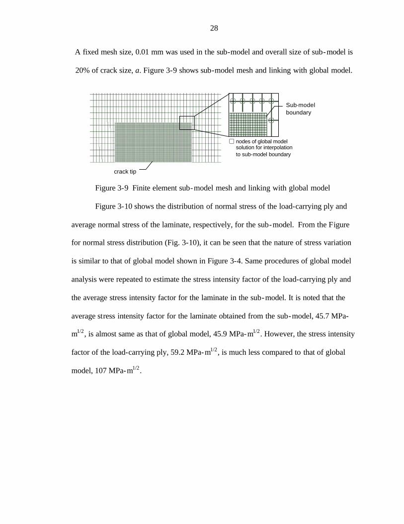
A fixed mesh size, 0.01 mm was used in the sub-model and overall size of sub-model is
20% of crack size, a. Figure 3-9 shows sub-model mesh and linking with global model.
Figure 3-9 Finite element sub-model mesh and linking with global model
Figure 3-10 shows the distribution of normal stress of the load-carrying ply and
average normal stress of the laminate, respectively, for the sub-model. From the Figure
for normal stress distribution (Fig. 3-10), it can be seen that the nature of stress variation
is similar to that of global model shown in Figure 3-4. Same procedures of global model
analysis were repeated to estimate the stress intensity factor of the load-carrying ply and
the average stress intensity factor for the laminate in the sub-model. It is noted that the
average stress intensity factor for the laminate obtained from the sub-model, 45.7 MPa-
m1/2, is almost same as that of global model, 45.9 MPa-m1/2. However, the stress intensity
factor of the load-carrying ply, 59.2 MPa-m1/2, is much less compared to that of global
model, 107 MPa-m1/2.
Sub-model boundary
nodes of global model solution for interpolation to sub-model boundary
crack tip

29
0.00E+00
2.00E+09
4.00E+09
6.00E+09
8.00E+09
1.00E+10
0.00E+00 1.00E-04 2.00E-04 3.00E-04 4.00E-04 5.00E-04
Figure 3-10 Normal stress distribution in the sub-model in case of [0/±45]s laminate
0.00E+00
2.00E+07
4.00E+07
6.00E+07
8.00E+07
1.00E+08
1.20E+08
0.00E+00 1.00E-04 2.00E-04 3.00E-04 4.00E-04 5.00E-04
Figure 3-11 Stress intensity factor in the sub-model in case of [0/±45]s laminate
Lyσ in the load-carrying ply Lxσ in the load-carrying ply
yσ in the laminate
xσ in the laminate
rLy πσ 2 in the load-carrying ply
ry πσ 2 in the laminate
Extrapolation line y = 9.73E+10x + 5.92E+07
Extrapolation line y = 7.52E+10x + 4.57E+07
Distance from crack tip, r (m)
N
orm
al s
tres
s, (
MP
a)
Distance from crack tip, r (m)
S
tres
s In
tens
ity fa
ctor
,
(MP
a-m
1/2
)
30
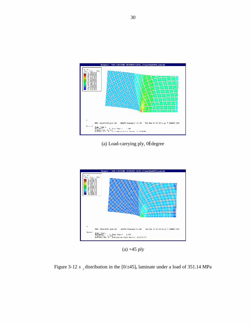
(a) Load-carrying ply, 0Edegree
(a) +45 ply
Figure 3-12 yσ distribution in the [0/±45]s laminate under a load of 351.14 MPa

31
3.3 Comparison of FE Results and Analytical Model
The stress intensity factor in the load-carrying ply was calculated using both the
global and sub-model. The laminate stress intensity factors calculated from the two
models were in good agreement for all laminate configurations indicating that the mesh
refinement was sufficient. From the laminate stress intensity factor, we can calculate the
finite-width correction factor Y using the relation
aYK yQ πσ ∞= (16)
The values of Y for various laminate configurations are shown as a function of
a/w and β in Figure 3-21. It has been found that the finite-width correction factor is a
strong function of the newly introduced lamination parameter β . More on this effect and
significance of β will be presented in Chapter 3.4. The results for the load-carrying ply
stress intensity factor yielded some interesting trends. The results of LQK estimated
through the finite element analysis are shown in Figure 3-16 and compared with two
analytical models. The LBQK )( calculated from Eq. (15) agrees well with the results of the
global model, which has a relatively coarse mesh. On the other hand, the LAQK )(
calculated from the exact LEFM solution, Eq. (14), shows good agreement with the
results of sub-model, which has a very fine mesh. It is obvious from the results that the
xσ stresses ahead of the crack tip play a significant role in the estimation of LQK . The
coarse mesh of global model does not have sufficient nodes to capture the xσ effect,
although it is good enough for determining yσ . The global model is not able to present a
complete picture of stresses in the vicinity of the crack tip.

32
0.00E+00
2.00E+09
4.00E+09
6.00E+09
8.00E+09
1.00E+10
0.00E+00 1.00E-04 2.00E-04 3.00E-04 4.00E-04 5.00E-04
global model
global model
sub-model
sub-model
Figure 3-13 Comparison of normal stress distribution in the sub-model and global model in case of [0/±45]s laminate
0.00E+00
5.00E+07
1.00E+08
1.50E+08
2.00E+08
2.50E+08
3.00E+08
0.00E+00 2.00E-03 4.00E-03 6.00E-03 8.00E-03 1.00E-02 1.20E-02 1.40E-02
global model
global model
Figure 3-14 Stress intensity factor in the global model in case of [0/±45]s laminate
Lyσ in global model Lxσ in global model Lyσ in sub-model Lxσ in sub-model
Distance from crack tip, r (m)
N
orm
al s
tres
s, (
MP
a)
Distance from crack tip, r (m)
S
tres
s In
tens
ity fa
ctor
,
(MP
a-m
1/2
)
Extrapolation line y = 1.17E+10x + 1.07E+08
Extrapolation line y = -5.44E+08x + 1.35E+07
rLy πσ 2 in global model
βπσ /2 rLx
in global model

33
0.00E+00
2.00E+07
4.00E+07
6.00E+07
8.00E+07
1.00E+08
1.20E+08
0.00E+00 1.00E-04 2.00E-04 3.00E-04 4.00E-04 5.00E-04
sub-model
sub-model
Figure 3-15 Stress intensity factor in the sub-model in case of [0/±45]s laminate
0
20
40
60
80
100
120
140
160
S1 S2 S3 S4 S5 S6 S7 S8 S9
sun ourglobal model submodel
Figure 3-16 Comparisons of the fracture toughness of principal load-carrying ply
Laminate configuration
Eq. (15) Eq. (14)
F
ract
ure
toug
hnes
s,
(MP
a-m
1/2
)
Distance from crack tip, r (m)
S
tres
s In
tens
ity fa
ctor
,
(MP
a-m
1/2
)
Extrapolation line y = 9.73E+10x + 5.92E+07
Extrapolation line y = -1.21E+11x + 6.03E+07
rLy πσ 2 in sub-model
βπσ /2 rLx
in sub-model
LBQK )(
LAQK )(

34
3.4 Finite-Width Correction (FWC) Factor
3.4.1 Isotropic Finite-Width Correction Factor
The lay-up independent failure model presented in Ref. [11] enables the
prediction of the notched strength of composite laminates. This model was formulated
assuming that the plates are of infinite width, thus, the infinite width notched strength,
∞Nσ , is predicted. However, experimental data provide notched strength data on finite
width specimens, Nσ . To account for finite width of the specimen, the finite-width
correction (FWC) factor Y is required to estimate the stress intensity factor accurately.
According to the definition, the finite-width correction factor is a scale factor, which is
applied to multiply the notched infinite solution to obtain the notched finite plate result.
A common method used extensively in the literature is to relate experimental notched
strength, Nσ , for plates of finite width to the notched strength of plates of infinite width
is to simply multiply Nσ by the finite-width correction factor Y, where IK is the mode I
stress intensity factor.
∞∞ =
I
INN K
Kσσ (17)
The mode I critical stress intensity factor for isotropic plate of finite width is
calculated from following equation.
aYK NISOQ πσ= (18)
Due to the lack of an analytical expression for orthotropic or anisotropic finite-width
correction factors, the existing lay-up independent failure models used isotropic finite-
width correction factor, YISO , to evaluate stress intensity factor of notched composite

35
laminates. Usually YISO is a 3rd order polynomial in a/w, which was developed
empirically for the case of center cracks in isotropic panels. For example
32 )/(5254.1)/(2881.0)/(1282.01 wawawaYISO +−+= (19)
can be found in Ref. [11]
However, the isotropic finite-width correction factor does not properly account
for the anisotropy exhibited by different laminate configuration. In some cases, the
application of the isotropic finite-width correction factors to estimate the anisotropic or
orthotropic finite-width correction factors can cause significant error.
3.4.2 Orthotropic Finite-Width Correction Factor
3.4.2.1 Developing procedure for FWC solution
To improve the accuracy of notched strength predictions for finite-width notched
composite laminates, orthotropic finite-width correction factor is obviously required.
There are a couple of methods to determine the orthotropic finite-width correction factor
[13-15]. However, no closed form solution is available. For this purpose, closed form of
orthotropic finite-width correction factor is developed empirically based on the results of
finite element analysis. It is found that Y depends on ß also.
The finite-width correction factor for orthotropic plate can be obtained from
following equation, where )0,(xy∞σ is the normal stress distribution in an infinite plate.
aK
Yy
IOT
πσ 2∞= (20)
where ∞yσ is the remote uniaxial stress, and a is the half crack length.
However, a closed form expression for IK does not exist. To estimate values of
IK for various laminate configurations, the commercial finite element code, ABAQUS

36
6.2/Standard, was used. The stress intensity factor, KI, can be calculated in two different
ways based on the finite element analysis as mentioned earlier.
The accuracy of these methods is investigated by comparison between a known
closed form solution Eq. (19) for notched isotropic plate and the solution obtained from
ABAQUS finite element models. In the finite element analysis, eight node, plane stress
elements were used to model notched plates made from isotropic material with material
property E = 100 GPa and v = 0.25. Geometry and mesh size of the global model were
used to evaluate the J- integral for the range of crack sizes given by wa / = 0.05, 0.1, 0.2,
0.2625 (specimen), 0.3, 0.4, 0.5. Ten contour lines were used to evaluate the J- integral in
the finite element models. Each contour is a ring of elements completely surrounding the
crack tip starting from one crack face and ending at the opposite crack face. These rings
of elements are defined recursively to surround all previous contours. ABAQUS 6.2
automatically finds the elements that form each ring from the node sets given as the
crack-tip or crack-front definition. Each contour provides an evaluation of the J- integral
Figure 3-17 shows the estimated finite-width correction factor determined by
finite element methods and a closed form solution for an isotropic notched plate with
various notch sizes. Excellent agreement between these analysis methods is noted over
the whole notch size of the plate.

37
0.95
1.00
1.05
1.10
1.15
1.20
0.00 0.05 0.10 0.15 0.20 0.25
Finite Element J-Integral
Finite Element Stress
Closed form solution
Figure 3-17 Comparison of the finite-width correction factors in an isotropic plate computed by the finite element methods with the closed form solution
The most accurate method, finite element J- integral, was adopted to develop the
finite-width correction factor for orthotropic plates. Figure 3-18 shows the calculated J-
integral value from FE global model for the material and lay-ups in Table 2-1. Ten
contour lines were used to evaluate J- interagl and these values are reasonably
independent of the path as expected. The first four J- integral values were taken to
calculate average J- integral and it was used to estimate KI using Eq. (3). The orthotropic
finite-width correction factor obtained using Eq. (20) are shown in Figure 3-19. As
expected, the finite-width correction factors increase with the crack size to panel width
ratio. Additionally, the finite-width correction factor strongly depends on the anisotropy
of laminate characterized by ß. Figure 3-20 shows the finite-width correction factor for
different values of anisotropy parameter β and the β values of laminated composite
panel using Eq. (6) are shown in Table 3-2.
a/w
Fin
ite-w
idth
cor
rect
ion
fact
or
Standard Deviation ¡ 0.107 % r 0.461 %
Intensity Factor

38
0.00E+00
2.00E+02
4.00E+02
6.00E+02
8.00E+02
1.00E+03
1.20E+03
1 2 3 4 5 6 7 8 9 10
a/w=10%
a/w=20%
a/w=26%
a/w=30%
a/w=40%
a/w=50%
Figure 3-18 J-integral vs. contour line calculated from FE model of the [0/±45]s laminate
Table 3-1 J- integral value calculated from FE model of the [0/±45]s laminate
Crack size (a/w) 0.1 0.2 0.26 0.3 0.4 0.5
Contour 1 1.31E+02 2.72E+02 3.75E+02 4.44E+02 6.71E+02 9.63E+02
Contour 2 1.31E+02 2.81E+02 3.88E+02 4.59E+02 6.82E+02 9.75E+02
Contour 3 1.31E+02 2.81E+02 3.88E+02 4.59E+02 6.82E+02 9.75E+02
Contour 4 1.26E+02 2.81E+02 3.88E+02 4.59E+02 6.82E+02 9.75E+02
Contour 5 1.29E+02 2.81E+02 3.88E+02 4.59E+02 6.82E+02 9.75E+02
Contour 6 1.37E+02 2.70E+02 3.88E+02 4.59E+02 6.82E+02 9.75E+02
Contour 7 1.48E+02 2.76E+02 3.73E+02 4.59E+02 6.82E+02 9.75E+02
Contour 8 1.64E+02 2.87E+02 3.81E+02 4.41E+02 6.82E+02 9.75E+02
Contour 9 1.75E+02 3.16E+02 3.96E+02 4.44E+02 6.55E+02 9.75E+02
Contour 10 1.97E+02 3.38E+02 4.04E+02 4.59E+02 6.60E+02 9.75E+02
Contour line
J-in
tegr
al
Crack size

39
1.00
1.10
1.20
1.30
1.40
1.50
0.00 0.10 0.20 0.30 0.40 0.50
isotropic
[0/±45]s
[0/±15]s
[0/±30]s
[0/90]2s
[±45/0/±45]s
[±45/±45/0/±45]s
[0/90/±45]s
[90/0/±45]s
Figure 3-19 The finite-width correction factors vs. ratio of crack size to panel width
1
1.1
1.2
1.3
1.4
1.5
0.1 0.3 0.5 0.7 0.9
2a/w=0.22a/w=0.262a/w=0.32a/w=0.42a/w=0.5
Figure 3-20 The finite-width correction factors vs. anisotropy parameter, β
Fin
ite-w
idth
cor
rect
ion
fact
or
Anisotropy parameter, β
a/w
Fin
ite-w
idth
cor
rect
ion
fact
or
S4
S5
S6 S8 S9 S1,2,3,7

40
Table 3-2 Values of the anisotropy parameter, ß, for the test specimens
specimen S1 S2 S3 S4 S5 S6 S7 S8 S9
β 1 1 1 0.285 0.396 0.656 1 0.767 0.823
The above results indicated that there is a definite relation between the finite-
width correction factors, geometric parameter, a/w, and anisotropy parameter, β . Thus,
the general semi-empirical solution of orthotropic finite-width correction factor was
developed using multiple least square regressions to fit measured data in the finite
element analysis. It can be expressed in terms of ß and ratio of crack size, a/w, in the
following form
( ) )1()1(11 265
3
32
43
2
22
211 BcBcwa
bBcBcwa
bBcBcwa
bYOT ++
+++
+++
+= (21)
where B is defined as 1- β , and the coefficients of least square fit are shown in Table 3-3.
A 3D plot of the finite-width correction factors is given in Figure 3-21 and estimated
values of the factor are summarized in Table 3-4. Note that YOT increases with a/w and
B.
Table 3-3 The coefficients of semi-empirical solution of orthotropic finite-width correction factor
b1 c1 c2 b2 c3 c4 b3 c5 c6
0.1091 5.0461 -2.1324 -0.2319 -2.9103 -4.4927 1.4727 -1.5124 -0.0375

41
Figure 3-21 The finite-width correction factors as a function of anisotropy parameter, ß, and ratio of crack size to panel width, a/w.
Table 3-4 The finite-width correction factors obtained from the semi-empirical solution (Eq. 21)
Orthotropic, YOT Isotropic, a/w
S1 S2 S3 S4 S5 S6 S7 S8 S9 YISO
0.10 1.011 1.011 1.011 1.046 1.041 1.029 1.010 1.023 1.020 1.01
0.20 1.024 1.024 1.024 1.107 1.094 1.065 1.024 1.052 1.045 1.02
0.26 1.040 1.040 1.040 1.152 1.134 1.092 1.040 1.075 1.066 1.04
0.30 1.051 1.051 1.051 1.182 1.160 1.111 1.052 1.091 1.082 1.05
0.40 1.101 1.101 1.101 1.269 1.239 1.173 1.101 1.148 1.136 1.10
0.50 1.181 1.181 1.181 1.369 1.331 1.254 1.181 1.227 1.214 1.18
42
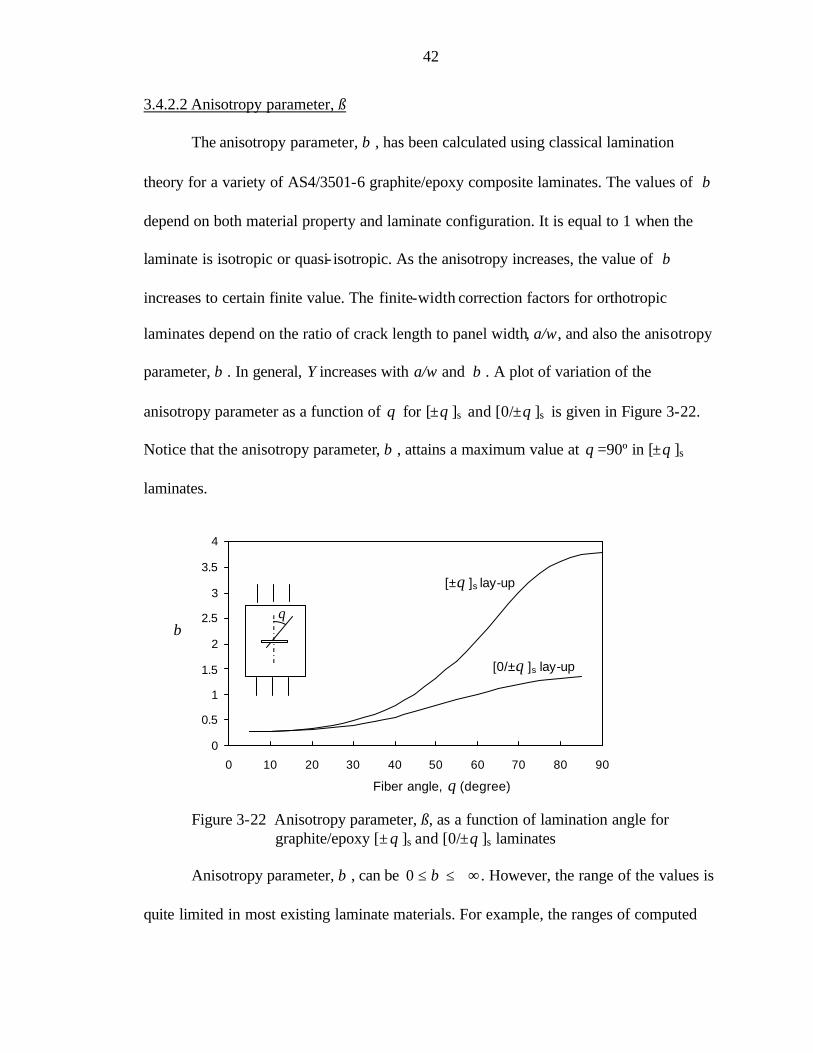
3.4.2.2 Anisotropy parameter, ß
The anisotropy parameter, β , has been calculated using classical lamination
theory for a variety of AS4/3501-6 graphite/epoxy composite laminates. The values of β
depend on both material property and laminate configuration. It is equal to 1 when the
laminate is isotropic or quasi- isotropic. As the anisotropy increases, the value of β
increases to certain finite value. The finite-width correction factors for orthotropic
laminates depend on the ratio of crack length to panel width, a/w, and also the anisotropy
parameter, β . In general, Y increases with a/w and β . A plot of variation of the
anisotropy parameter as a function of θ for [±θ ]s and [0/±θ ]s is given in Figure 3-22.
Notice that the anisotropy parameter, β , attains a maximum value at θ =90º in [±θ ]s
laminates.
0
0.5
1
1.5
2
2.5
3
3.5
4
0 10 20 30 40 50 60 70 80 90
Figure 3-22 Anisotropy parameter, ß, as a function of lamination angle for graphite/epoxy [± θ ]s and [0/±θ ]s laminates
Anisotropy parameter, β , can be +∞≤≤ β0 . However, the range of the values is
quite limited in most existing laminate materials. For example, the ranges of computed
Fiber angle, θ (degree)
θ β
[0/±θ ]s lay-up
[±θ ]s lay-up
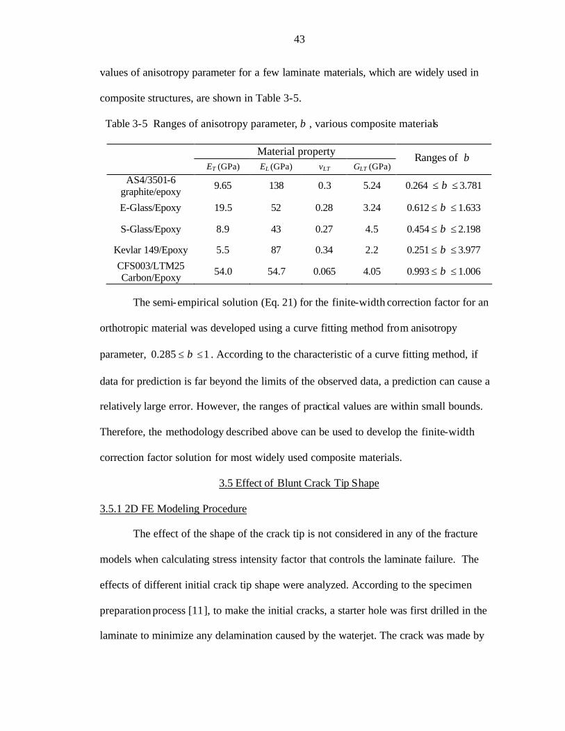
43
values of anisotropy parameter for a few laminate materials, which are widely used in
composite structures, are shown in Table 3-5.
Table 3-5 Ranges of anisotropy parameter, β , various composite materials
Material property
ET (GPa) EL (GPa) vLT GLT (GPa) Ranges of β
AS4/3501-6 graphite/epoxy 9.65 138 0.3 5.24 0.264 ≤≤ β 3.781
E-Glass/Epoxy 19.5 52 0.28 3.24 0.612 ≤≤ β 1.633
S-Glass/Epoxy 8.9 43 0.27 4.5 0.454 ≤≤ β 2.198
Kevlar 149/Epoxy 5.5 87 0.34 2.2 0.251 ≤≤ β 3.977
CFS003/LTM25 Carbon/Epoxy 54.0 54.7 0.065 4.05 0.993 ≤≤ β 1.006
The semi-empirical solution (Eq. 21) for the finite-width correction factor for an
orthotropic material was developed using a curve fitting method from anisotropy
parameter, 1285.0 ≤≤ β . According to the characteristic of a curve fitting method, if
data for prediction is far beyond the limits of the observed data, a prediction can cause a
relatively large error. However, the ranges of practical values are within small bounds.
Therefore, the methodology described above can be used to develop the finite-width
correction factor solution for most widely used composite materials.
3.5 Effect of Blunt Crack Tip Shape
3.5.1 2D FE Modeling Procedure
The effect of the shape of the crack tip is not considered in any of the fracture
models when calculating stress intensity factor that controls the laminate failure. The
effects of different initial crack tip shape were analyzed. According to the specimen
preparation process [11], to make the initial cracks, a starter hole was first drilled in the
laminate to minimize any delamination caused by the waterjet. The crack was made by

44
waterjet cut and further extended with a 0.2mm thick jeweler’s saw blade. Thus, in the
present analysis, the crack tip thickness was assumed less than 0.2mm and three different
crack tip shapes, elliptical, triangle, and rectangular, were considered. These assumptions
were carefully investigated through the series of FE sub-models and the results are
discussed below for the case of [0/±45]s laminate.
Figure 3-23 Crack tip shape profiles
3.5.2 Results and Discussion
Figures 3-24 and 3-25 compare the effect of crack tip profile and crack thickness
on the stress intensity factor of principal load-carrying ply using global and sub-model. In
this analysis, thickness of the crack was assumed to be less than 0.2 mm. The global
nature of FE models requires that the details of the crack tip shape are not explicitly
modeled due to the mesh size. Therefore, the global model may not accurately capture the
details near the crack tip and is not reliable in capturing the behavior of the crack tip
shape. From the results of the global model, it is evident that stress intensity factors of
global model are not greatly influenced by crack tip shape.

45
40
50
60
70
80
90
100
110
120
0 0.05 0.1 0.15 0.2 0.25
rectangle
semi-circle
triangle h/c=2
triangle h/c=1
Figure 3-24 Effect of crack tip shape on predicted fracture toughness of [0/±45]s laminate ; 2D FE global model results
20
30
40
50
60
70
80
90
100
110
120
0 0.05 0.1 0.15 0.2 0.25
rectanglesemi-circletriangle h/c=2triangle h/c=1
Figure 3-25 Effect of crack tip shape on predicted fracture toughness of [0/±45]s laminate ; 2D FE sub-model results
Crack thickness, 2h
F
ract
ure
toug
hnes
s,
(MP
a-m
1/2 )
Crack thickness, 2h
F
ract
ure
toug
hnes
s,
(MP
a-m
1/2 )
46
However, the results of the sub-model indicate that the crack tip shape has a
significant effect on the stress intensity factor at the crack tip. Furthermore, the large
variation was observed in the results shown in Figure 3-25. It indicates that the stress
intensity factor is very sensitive to the crack tip slope ahead of the crack tip. The results
shows that the crack tip slope near the crack tip is a more critical parameter than the
crack tip thickness. The results clearly indicate that the stress intensity factors at the crack
tip are strongly affected by the behavior of the crack tip shape.
3.6 Effect of Local Damage
The complicated nature of fracture behavior in notched composite laminates
makes it difficult to predict the exact position and size of every fiber break, matrix crack,
and delamination even in a relatively simple notched panel studied here. The philosophy
is not to model exactly, but to make approximations that agree well with actual behavior.
The objective of this section is to study the effect of damage in the vicinity of
crack tip such as delamination and fiber splitting by comparing stress intensity factor
computed using the three-dimensional FE analysis. It has been noted that for a tension
loaded laminate, local damage is produced ahead of the crack tip in the form of the
matrix cracks in off-axis plies, splitting in 0E plies and some delamination [11]. This
local damage acts as a stress-relieving mechanism and relieves some portion of the high
stress concentrated around the crack tip. This damage, such as matrix cracking and
delamination, may significantly affect the structural integrity of the structures when they
become sufficiently severe. However, failure models discussed in the previous section do
not represent any effects of local damage. Axial splitting and delamination are the most
common types of damage in laminated fiber reinforced composites due to the ir relatively

47
weak interlaminar strengths.
Previous finite element analysis used plane stress element in two-dimensional
modeling. Therefore, the effect of delamination between plies in the thickness direction
can not be modeled. In present finite element models, three-dimensional analysis was
adopted to investigate the effect of delamination and axial splitting using twenty node,
solid element (C3D20R element). Typically, solid element with reduced integration, is
used to form the element stiffness for more accurate results and reduce running time.
Sub-modeling analysis can be applied to shell-to-solid sub-model, however, the z-
direction (thickness direction) stress and strain field can not be interpolated to 3D solid
sub-model boundary from 2D global model. Thus, 3D global models were modeled to
analyze 3D sub-model with local damage. Figure 3-26 shows the Von-Mises stress
distribution in the [0/±45]s laminate of 3D global model and 3D sub-model. It should be
noted that before interpolating the results of the 3D global model, the comparison
between the results of 2D global model and 3D global model should be checked for
consistent analysis. In Figure 3-27, the estimated stress intensity factors in the load-
carrying ply from 3D global model are compared with those of 2D global model. The
stress intensity factors obtained from 3D global model are slightly underestimated
compared to those of the 2D global-model, however, these estimated values are fairly
consistent for the nine laminate configurations. Consequently, two types of damage were
modeled using 3D sub-model to predict the effect of local damage on the stress intensity
factor of the load-carrying ply.

48
(a) 3D global model
(b) 3D sub-model
Figure 3-26 Von-Mises stress distribution in [0/"45]s laminate

49
0
20
40
60
80
100
120
140
S1 S2 S3 S4 S5 S6 S7 S8 S9
2D global model 3D global model
Figure 3- 27 Comparison of stress intensity factor of the load-carrying ply between 2D and 3D global model
3.6.1 3D FE Modeling Procedure for Delamination
All aspects of the finite element model were kept the same as 3D sub-model
except interface of ply. Each ply was modeled by four elements through the thickness as
shown in Figure 3-26(b). Elements of layers are connected through either side of any ply
interfaces at common nodes except where delamination is expected. The delamination
was modeled as separate, unconnected nodes with identical coordinates. Figure 3-28
show the schematic of ply interface mesh where delamination is expected. To estimate
delamination area, a simple delamination criterion was implemented in ABAQUS by
means of a UVAR user subroutine using the following equation.
Delamination area : Tzzyzxz S≤++ 222 σττ (22 )
where ST is critical stress of matrix which is 75 MPa based on typical epoxy yield
strength. Figure 3- 29 shows the estimated delamination area using the above
Laminate configuration
Str
ess
inte
nsity
fact
or,
(MP
a-m
1/2
)

50
delamination criterion in the ply between the load-carrying ply and +45E ply of [0/±45]s
laminate.
(a) no damage (b) delamination
Figure 3-28 Scheme of ply interface mesh in the [0/±45]s laminate
Figure 3-29 Estimated delamination area on interface between 0E and +45E ply in the [0/±45]s laminate
crack line

51
3.6.2 3D FE Modeling Procedure for Axial Splitting
When a notched composite panel is subjected to tension loading axial splitting
occurs in the crack tip area due to high stress concentration and low matrix tensile
strength. Apparently, this failure mode causes severe stiffness reduction in transverse
direction. Thus, transverse stiffness of axial splitting area can be modeled by taking
0≈TE . This failure mode and assumption are illustrated in Figure 3-30. Similar method
described in the previous section was used to estimate axial splitting area where reduced
stiffness property was implemented, ET =10 Pa that is extremely small compared to initial
modulus, ET =9.65 GPa. A critical stress of 75 MPa was used, based on a typical epoxy
yield stress. Figure 3-31 shows the estimated axial splitting area in the interface between
0E and +45E ply for a tensile loading 351.14 MPa.
Figure 3-30 Axial splitting failure mode in the load-carrying ply

52
Figure 3-31 Estimated axial splitting area on interface between 0E and +45E ply 3.6.3 Results and Discussion Typical damage in notched laminated composites occurs in the form of axial
splitting in the load-carrying ply and delamination. This damage was modeled to study
effect of local damage on the normal stress distribution in the vicinity of crack tip in the
load-carrying ply. The estimated delamination area and axial splitting area are modeled
by having duplicate nodes and reduced stiffness, respectively.
Results of normal stress distribution are shown in Figure 3-32. From the results it
is observed that s y distribution in the FE model without damage shows the typical square
root singularity. Axial splitting and delamination removes the singularity, though there
still is a region of high stress concentration near the crack tip. It also can be seen that yσ
distribution increases away from the crack tip and xσ distribution in the model with
damage decreases than in the model with no damage. Thus, the stress field is strongly
affected by the presence of local damage. From the results, it is obvious that the local
crack line

53
damage serve as main mechanism to increase yσ distribution and decreases xσ
distribution in the load-carrying ply. This simulation is similar to the redistribution of
stress in the presence of small scale yielding in homogenous materials.
0.00E+00
2.00E+09
4.00E+09
6.00E+09
8.00E+09
1.00E+10
0.00E+00 1.00E-04 2.00E-04 3.00E-04 4.00E-04 5.00E-04
with no damage
with no damage
with damage
with damage
Figure 3-32 Effect of the local damage on normal stress distribution in the load- carrying ply in the [0/±45]s laminate
3.7 Summary of FE Results and Discussion
It is well established that the fracture behavior of composite laminates depends on
a variety of variables. All may affect to varying degrees the fracture behavior of the
notched laminates. A comprehensive evaluation is still lacking regarding the effects of all
variables on the notch sensitivity of composite laminates. Through the detailed finite
element analysis, we investigated effect of distinct factors such as crack tip shape and
local damage.
The presence of blunt crack tip has a significant effect on the behavior of notched
composites, and leads to stress redistribution. This relives the stresses in the non- load-
carrying plies and increases the SIF of the load-carrying plies. Similar effects are
observed when local damage such as matrix cracking and delamination are introduced.
s y s x
s y s x
Distance from crack tip, r (m)
N
orm
al s
tres
s, (M
Pa)

54
Figure 3-33 shows the results of finite element sub-model, which include blunt crack tip
and local damage. From the comparison of the results between models with and without
damage, it is obvious that these effects also increase the stress intensity factor of the load-
carrying ply as a result of the reduction in xσ stress concentration in the laminate. By
comparing the results of finite element analysis with analytical failure model, it can be
reasonably assumed that the effect of initial damage is accounted by reducing the
xσ component ahead of crack tip to zero.
0
20
40
60
80
100
120
140
S1 S2 S3 S4 S5 S6 S7 S8 S9
no damage in 3D sub-model damage in 3D sub-model
Figure 3-33 Effect of the local damage on stress intensity factor in the load- carrying ply
Laminate configuration
F
ract
ure
toug
hnes
s,
MP
a-m
1/2

55
CHAPTER 4 CONCLUSIONS AND FUTURE WORK
CONCLUSIONS
The SIF of the load-carrying ply is a critical parameter for predicting the failure of
notched composite laminates. The SIF of the load-carrying ply, LQK , can be estimated by
using a detailed 3D FE analysis which can model local damage modes such as fiber
splitting and delamination that occurs prior to fracture. Then the SIF of the load-carrying
ply can be calculated accurately and compared with the critical value for the material
system to predict fracture. The results from this model are presented in Column 2 of
Table 4-1.
On the other hand, a simpler analytical model could be used. In this model finite-
width correction factor for orthotropic laminates should be used. The effects of local
damage at the crack tip is accounted for by setting the parameter β=0 in Eq. (15) for
calculating the SIF of the load-carrying ply. Results from such analysis are shown in
Column 3 of Table 4-1. The results from calculations performed by Sun and Vaiday [11]
are given in Column 4 for comparison.
Using a mean value of 113.81 MPa-m1/2 for LQK in the analytical model, the
predictions of the laminate fracture toughness are compared with the experimental results
in Figure 4-2 for various value of η .

56
0
20
40
60
80
100
120
140
S1 S2 S3 S4 S5 S6 S7 S8 S9
Figure 4-1 Comparison of the fracture toughness of load-carrying ply
Table 4-1 Comparison of the fracture toughness of load-carrying ply obtained from different methods
Fracture toughness of load-carrying ply, L
QK , MPa-m1/2
Specimen 3D FE analysis Analytical model
Ref. [11]
S1 116.65 115.66 115.66 S2 114.23 108.82 108.82 S3 115.71 106.43 106.43 S4 118.16 112.62 101.81 S5 115.21 109.97 101.00 S6 113.53 111.52 106.32 S7 121.40 109.04 109.04 S8 116.01 123.66 119.81 S9 110.51 126.58 123.64
average 115.71 113.81 110.28 S.D.† 3.03 % 6.95 % 9.80 %
† standard deviation
Analytical model
LAQK )(
3D FE analysis
Laminate configuration
F
actu
re to
ughn
ess,
(M
Pa-
m1
/2)

57
The variable η was defined as ratio of stress intensity factor of the load-carrying
ply to that of laminate and can be obtained from Eq. (15). It should be noted that ?, like ß,
depends entirely on the laminate properties. Good agreement is observed between the
experiments and predictions. By comparison with experimental results, it is concluded
that the proposed lay-up independent model with orthotropic finite-width correction
factor is capable of predicting fracture toughness of notched laminated composites with
reasonable accuracy for mode I loading.
S9
0
20
40
60
80
100
120
140
160
0 0.5 1 1.5 2 2.5 3 3.5 4 4.5 5
S8S1S6
S7
S5S4
Predicted curve(analytical model)
S2S3
§ η is defined as [ ]*2222
*1212
)( AQAQtK
K LL
Q
LBQ +==η from Eq. (15)
Figure 4-2 Comparison of experimental results with failure model predictions
η §
Lam
inat
e fr
actu
re to
ughn
ess,
(M
Pa-
m1
/2)

58
1
1.2
1.4
1.6
1.8
2
2.2
2.4
0 0.1 0.2 0.3 0.4 0.5 0.6 0.7
experiment prediction
S4
S5S7
S6
S1
S2 S3
S8 S9
Figure 4-3 Comparison of experimental results with failure model predictions
(log scale)
Table 4-2 Comparison of experimental results with failure model predictions
Specimen Fracture toughness of laminates, QK (MPa-m1/2)
Notation Lay-up η
Experiment† Prediction‡ Relative error (%)
S1 [0/90/±45]s 2.5791 44.67768 44.1295 1.23
S2 [±45/90/0]s 2.5791 40.22554 44.1295 -9.71
S3 [90/0/±45]s 2.5791 41.16729 44.1295 -7.20
S4 [0/±15]s 1.1209 100.4675 101.5384 -1.07
S5 [0/±30]s 1.6619 66.24291 68.48451 -3.38
S6 [0/±45]s 2.3215 48.07307 49.02623 -1.98
S7 [0/90]2s 1.8706 58.19245 60.84379 -4.56
S8 [±45/0/±45]s 3.1979 38.68474 35.59036 7.99
S9 [±452/0/±45]s 3.8168 33.19171 29.81933 10.16
† Fracture toughness of laminates obtained using Eq. (1) with orthotropic finite-width correction factor in Table 3-4. ‡ Predicted fracture toughness of laminates calculated using the mean value, 113.81 MPa-m1/2, for L
QK in the analytical model.
log(η )
log,
(KQ)

59
FUTURE WORK
There seems to be ample room for further investigation of this problem. Fracture
problem studied in the current study was limited to AS4/3501-6 graphite/epoxy laminated
panel containing a center straight crack subjected to tension loading. For general
application, validity of currently proposed lay-up independent criterion can be further
verified for the case of laminated composite panels containing double edge notch, single
edge notch, circular hole, etc. with different material systems using experimental and
numerical analyses for mode II and mixed loading conditions. Additionally, this failure
model can be compared with other popular failure models such as Point Stress Criterion,
Average Stress Criterion, Mar-Lin failure model, etc. so that composite structure
designers can select an appropriate failure model in diverse practical situations.

60
APPENDIX A LAMINATION THEORY
For laminated plates with bending-extension coupling under plane stress, the
complete set of force-mid-plane deformation equations can be expressed in matrix form
as
=
κε 0
||DBBA
MN (A-1)
where N and M are the in-plane forces and moments, respectively, and 0ε is the mid-
plane strains, and κ is the curvature.
In the case of symmetric laminates without coupling, Eq. (A-1) is reduced to
=
0
0
0
662616
262212
161211
xy
y
x
zy
y
x
AAAAAAAAA
NNN
γεε
(A-2)
where the laminate extensional stiffness are given by
∫−=
2/
2/)(
t
t kijij dzQA (A-3)
where t is the thickness of the laminate. If there are N layers in the lay-up, we can rewrite
the above equations as a summation of integrals over the laminate. The material
coefficients will then take the form
∑=
−−=N
kkkkijij zzQA
11)()( (A-4)

61
Figure A-1 Laminated plate geometry
where the kz and 1−kz in these equation indicate that the k th lamina is bounded by
surfaces kz and 1−kz . Thus, the ijQ depend on the material properties and fiber
orientation of the k th layer. It can be obtained using the following equation.
[ ] [ ] [ ] [ ] [ ] [ ]11 −−= RTRQTQ (A-5)
where
−−−=
22
22
22
22][
nmmnmnmnmn
mnnmT , [ ]
=
200010
001
R (A-6)
m=cosθ and n=sinθ
where the ijQ are the components of the transformed lamina stiffness matrix which are
defined as follows
θθθθ 226612
422
41111 cossin)2(2sincos QQQQQ +++=
)cos(sincossin)4( 4412
2266221112 θθθθ ++−+= QQQQQ
θθθθ 226612
422
41122 cossin)2(2cossin QQQQQ +++=
θθθθ cossin)2(cossin)2( 3662212
366121116 QQQQQQQ +−+−−=
θθθθ 3662212
366121126 cossin)2(cossin)2( QQQQQQQ +−+−−=
)cos(sincossin)22( 4466
226612121166 θθθθ ++−−+= QQQQQQ (A-7)

62
=
zy
y
x
xy
y
x
NNN
AAAAAAAAA
*66
*26
*16
*26
*22
*12
*16
*12
*11
0
0
0
γεε
(A-8)
where superscript * denotes the component of inverse matrix of [ ]A
The stresses in each ply can be recovered form the mid-plane strains. In particular,
the stresses in the load-carrying ply can be expressed as
=
0
0
0
662616
262212
161211
xy
y
x
LLL
LLL
LLL
Lxy
Ly
Lx
QQQQQQQQQ
γεε
τσσ
(A-9)
where superscript L means the component of principal load carrying ply
The normal stress field applied in the load-carrying ply can be obtained by
calculating the portion of the applied load that is carried by the load-carrying ply using
lamination theory using Eqs. (A-8) and (A-9).
=
xy
y
x
LLL
LLL
LLL
Lxy
Ly
Lx
NN
N
AAAAAA
AAA
QQQQQQ
QQQ
*66
*26
*16
*26
*22
*12
*16
*12
*11
662616
262212
161211
τσ
σ
(A-10)

63
APPENDIX B MATHEMATICAL THEORIES OF BRITTLE FRACTURE
The objective of this Appendix was to provide the brief review of mathematical
formulation of crack problems for derivation of stress intensity factor in homogeneous
orthotropic materials [17].
For orthotropic materials in the case of plane stress, the generalized Hooke law
can be expressed as
xyyyxxxy
xyyyxxyy
xyyyxxxx
aaa
aaa
aaa
τσσγ
τσσε
τσσε
662616
262212
161211
++=
++=
++=
(B-1)
0=== zyzxz σσσ
The equilibrium equations under plane stress conditions are
0=∂
∂+
∂∂
yxxyxx
τσ, 0=
∂
∂+
∂
∂
yxyyyx στ
(B-2)
The equilibrium equations will be satisfied if the stress function U(x,y) is
expressed as
2
2
yU
xx ∂∂
=σ , 2
2
xU
yy ∂∂
=σ , xy
Uxy ∂∂
∂−=
2
τ (B-3)
Substituting for xxσ , yyσ , xyτ from Eq. (B-3) in the compatibility equation
yxxyxyyyxx
∂∂
∂=
∂
∂+
∂∂ γεε
2
2
2
2
(B-4)

64
The governing characteristic equation of plane stress of orthotropic materials can
be expressed as
02)2(2 4
4
113
4
1622
4
661223
4
264
4
22 =∂∂
+∂∂
∂−
∂∂∂
++∂∂
∂−
∂∂
yU
ayxU
ayx
Uaa
yxU
axU
a (B-5)
Defining the operators Dj (j= 1, 2, 3, 4) as
xyD jj ∂
∂−
∂∂
= µ (j= 1, 2, 3, 4) (B-6)
The governing equation in U(x,y) becomes
D1 D2 D3 D4 U (x,y) = 0 (B-7)
and jµ are the roots of the characteristic equation.
02)2(2 22262
66123
164
11 =+−++− aaaaaa jjjj µµµµ (B-8)
The roots are either complex or purely imaginary and cannot be real and can be
expressed as
1111 δαµ is +== , 2222 δαµ is +== ,
13 uu = , 24 uu = (B-9)
where iα , jδ (j= 1, 2) are real constants.
The stress function U(x,y) can be expressed in the form
U(x,y)=2 Re [U1(z1)+U2(z2)] (B-10)
where U1(z1) and U2(z2) are the arbitrary functions of the complex variables ysxz 11 +=
and ysxz 22 += , respectively. Let new functions
111 /)( dzdUz =φ , 222 /)( dzdUz =ψ (B-11)
Substituting the stress function from Eq. (B-10) into the Eq. (B-3) and taking into
account the relations in Eq. (B-11), the stress components can be expressed as

65
)](')('Re[2
)](')('Re[2)]('2)('2Re[2
2211
21
2221
21
zszs
zzzszs
xy
y
x
ψφτ
ψφσψφσ
+−=
+=+=
(B-12)
For pure mode I case, the stress components in the vicinity of crack tip can be
expressed in terms of stress intensity factor, KI , and the roots of characteristic Eq. (B-8)
+−
+−=
θθθθπσ
sincossincos
1Re
2 1
2
2
1
21 s
s
s
sssr
K Iy
+−
+−=
θθθθπσ
sincossincosRe
2 1
1
2
2
21
21
s
s
s
sss
ss
r
K Ix (B-13)
+−
+−=
θθθθπτ
sincos1
sincos1
Re2 2121
21
ssssss
rK I
xy
Figure B-1 Stress components in the vicinity of crack tip
when θ = 0, the new parameter ß introduced in the Chapter 2.3 can be expressed as (
( )( ) [ ]21Re
0,0, ss
rr
y
x −==σσβ (B-14)
Consequently, the model I stress intensity factor can be expressed as
rrK yrI πσ 2)0,(lim0→
= (B-15)

66
KI can also be expressed in terms of xσ as
β
πσ rrK
xrI
2)0,(lim0→= (B-16)
The increase in strain energy due to the presence of the crack can be calculated
using following equation for mode I case.
∫−
∆=∆a
ayyy dxuxW )0,(
21
σ (B-17)
The derivative of W∆ with respect to crack size, a, yield
+=
∂∆∂
21
2122
2 Ressss
iaKaW
I (B-18)
The energy release rate can be expressed in terms of stress intensity factor
+=
21
2122
2
Re2 ss
ssia
KG I
I (B-19)
where si (j = 1,2) are the roots of the characteristic equation (B-8) which can be derived
from the elastic constants as
2/1
11
2221
−=
aa
ss ,
2/1
11
6612
2/1
11
2221 2
22
++
=+
aaa
aa
iss (B-20)
Then, the relation equation between GI and KI for an orthotropic material can be
expressed as
2/1
11
6612
2/1
11
222/1
22112
22
2
++
=
aaa
aaaa
KG II (B-21)

67
LIST OF REFERENCES
[1] Awerbuch J, Madhukar M.S., “Notched strength of composite laminates: prediction and experiments-a review.” Journal of Reinforced Plastics and Composites 1985;4:3-159
[2] Waddoups M.E., Eisenmann J.R., Kaminski B.E., “Macroscopic fracture
mechanics of advanced composites materials.” Journal of Composites Materials 1971;5:446-54
[3] Whitney J.M., Nuismer R.J., “Stress fracture criteria for laminated composites
containing concentrations.” Journal of Composite Materials 1974;8:253-65. [4] Tan S.C., “Effective stress fracture models for unnotched and notched
multidirectional laminates.” Journal of Composites Material 1988;22:322-40. [5] Mar L.W., Lin K.Y., “Fracture mechanics correlation for tensile failure of
filamentary composites with holes.” Journal of Aircraft 1977;14:703-707 [6] Chang F.K., Chang K.Y., “Progressive damage model for laminated composites
containing stress concentration.” Journal of Composites Materials 1987;21:834-855
[7] Tan S.C., “A progressive failure model for composite laminates containing
openings.” Journal of Composites Materials 1991;25:556-577 [8] Poe C.C. Jr., “An unified strain criterion of fracture of fibrous composite
laminates.” Engineering Fracture Mechanics 1983;17:153-171 [9] Poe C.C. Jr., Sova J.A., “Fracture toughness of boron/aluminum laminates with
various proportions of 0E and ±45Eplies.” NASA Technical Paper 1707. Nov 1980
[10] Kageyama K., “Fracture mechanics of notched composite laminates.” Application
of Fracture Mechanics to Composites Materials 1989;327-396 [11] Sun C.T., Vaiday R.S., “Fracture criterion for notched thin composite laminates.”
AIAA Journal 1998;36:81-8. [12] Sun C.T., Vaiday R.S., Klug J.C., “Effect of ply thickness on fracture of notched
composite laminates.” AIAA Journal 1988;36:81-8.

68
[13] Tan S.C., “Finite-width correction factors for anisotropic plate containing a central opening.” Journal of Composite Materials 1998;22:1080-1098
[14] Naik N.K., Shembekar P.S., “Notched strength of fabric laminates.” Composites
Science and Technology 1992;44:1-12. [15] Gillespie, J.W. Jr., Carlsson L.A., “Influence of finite width on notched laminate
strength predictions.” Composites Science and Technology 1988;32:15-30 [16] Wisnom M.R., Chang F.K., “Modeling of splitting and delamination in notched
cross-ply laminates.” Composites Science and Technology 2000;60:2849-2856 [17] Sih G.C., Liebowitz H., Fracture and an Advanced Treatise. Volume II
Mathematical Fundamentals edited by Liebowitz H. 1968, Academic Press, New York and London
[18] Hibbit, Karlsson, Sorensen, ABAQUS version 6.2 Theory Manual published by
Hibbit, Karlsson & Sorensen, Inc. 1998, U.S.A.
69
BIOGRAPHICAL SKETCH
Bokwon Lee was born on July 15, 1973, in Kyungki province, Republic of Korea,
as the second son of Jonghan Lee and Jongok Woo. He graduated from Korea Airforce
Academy with a B.S. degree in aeronautical engineering in March 1996. After
graduation, He worked at the 19th Fighter Wing, Jungwon, Republic of Korea, for 3 years.
After promotion to Captain, he worked for Airforce Logistics Command as a technical
assistant for tactical combat aircrafts.
He came to the University of Florida for his graduate study in August 2001 and
began his research with Dr. Bhavani V. Sankar in the Department of Mechanical and
Aerospace Engineering. He completed his master’s program in August 2003.