Modal Regression using Kernel Density Estimation: aReview

Yen-Chi Chen∗

Abstract

We review recent advances in modal regression studies using kernel density estima-tion. Modal regression is an alternative approach for investigating relationship betweena response variable and its covariates. Specifically, modal regression summarizes theinteractions between the response variable and covariates using the conditional modeor local modes. We first describe the underlying model of modal regression and itsestimators based on kernel density estimation. We then review the asymptotic prop-erties of the estimators and strategies for choosing the smoothing bandwidth. We alsodiscuss useful algorithms and similar alternative approaches for modal regression, andpropose future direction in this field.

1 Introduction

Modal regression is an approach for studying the relationship between a response variable

Y and its covariates X. Instead of seeking the conditional mean, the modal regression

searches for the conditional modes (Collomb et al., 1986; Lee, 1989; Sager and Thisted,

1982) or local modes (Chen et al., 2016a; Einbeck and Tutz, 2006) of the response variable

Y given the covariate X = x. The modal regression would be a more reasonable modeling

approach than the usual regression in two scenarios. First, when the conditional density

function is skewed or has a heavy tail. When the conditional density function has skewness,

the conditional mean may not provide a good representation for summarizing the relations

between the response and the covariate (X-Y relation). The other scenario is when the

conditional density function has multiple local modes. This occurs when the X-Y relation

∗Department of Statistics, University of Washington

1

arX

iv:1

710.

0700

4v2

[st

at.M

E]

7 D

ec 2

017

contains multiple patterns. The conditional mean may not capture any of these patterns so

it can be a very bad summary; see, e.g., Chen et al. (2016a) for an example. This situation

has already been pointed out in Tarter and Lock (1993), where the authors argue that we

should not stick to a single function for summarizing the X-Y relation and they recommend

looking for the conditional local modes.

Modal regression has been applied to various problems such as predicting Alzheimer’s

disease (Wang et al., 2017), analyzing dietary data (Zhou and Huang, 2016), predicting

temperature (Hyndman et al., 1996), analyzing electricity consumption (Chaouch et al.,

2017), and studying the pattern of forest fire (Yao and Li, 2014). In particular, Wang et al.

(2017) argued that the neuroimaging features and cognitive assessment are often heavy-tailed

and skewed. A traditional regression approach may not work well in this scenario, so the

authors propose to use a regularized modal regression for predicting Alzheimer’s disease.

The concept of modal regression was proposed in Sager and Thisted (1982). In this

pioneering work, the authors stipulated that the conditional (global) mode be a monotone

function of the covariate. Sager and Thisted (1982) also pointed out that a modal regression

estimator can be constructed using a plug-in from a density estimate. Lee (1989) proposed

a linear modal regression that combined a smoothed 0-1 loss with a maximum likelihood

estimator (see equation (7) for how these two ideas are connected). The idea proposed in

Lee (1989) was subsequently modified in many studies; see, e.g., Kemp and Silva (2012);

Krief (2017); Lee (1989, 1993); Lee and Kim (1998); Manski (1991); Yao and Li (2014).

The idea of using conditional local modes has been pointed out in Tarter and Lock (1993)

and the 1992 version of Dr. David Scott’s book Multivariate density estimation: theory,

practice, and visualization (Scott, 1992). The first systematic analysis was done in Einbeck

and Tutz (2006), where the authors proposed a plug-in estimator using a kernel density

estimator (KDE) and computed their estimator by a computational approach modified from

the meanshift algorithm (Cheng, 1995; Comaniciu and Meer, 2002; Fukunaga and Hostetler,

1975). The theoretical analysis and several extensions, including confidence sets, prediction

sets, and regression clustering were later studied in Chen et al. (2016a). Recently, Zhou and

Huang (2016) extended this idea to measurement error problems.

The remainder of this review paper is organized as follows. In Section 2, we formally

2

define the modal regression model and discuss its estimator by KDE. In Section 3, we review

the asymptotic theory of the modal regression estimators. Possible strategies for selecting

the smoothing bandwidth and computational techniques are proposed in Section 4 and 5,

respectively. In Section 6, we discuss two alternative but similar approaches to modal re-

gression – the mixture of regression and the regression quantization method. The review

concludes with some possible future directions in Section 7.

2 Modal Regression

For simplicity, we assume that the covariate X is univariate with a compactly supported

denisty function. Two types of modal regression have been studied in the literature. The

first type, focusing on the conditional (global) mode, is called uni-modal regression (Collomb

et al., 1986; Lee, 1989; Manski, 1991; Sager and Thisted, 1982). The other type, which finds

the conditional local modes, is calld multi-modal regression (Chen et al., 2016a; Einbeck and

Tutz, 2006).

More formally, let q(z) denote the probability density function (PDF) of a random vari-

able Z. We define the operators

UniMode(Z) = argmaxz

q(z)

and

MultiMode(Z) = {z : q′(z) = 0, q′′(z) < 0},

which return the global mode and local modes of the PDF of Z, respectively. Note that we

need q to be twice differentiable. Uni-modal regression searches for the function

m(x) = UniMode(Y |X = x) = argmaxy

p(y|x) (1)

whereas multi-modal regression targets

M(x) = MultiMode(Y |X = x) =

{y :

∂

∂yp(y|x) = 0,

∂2

∂y2p(y|x) < 0

}. (2)

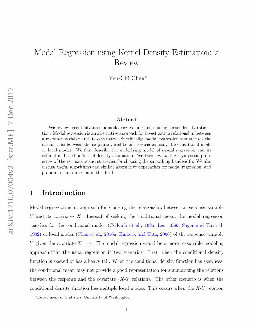
Note that the modal function M(x) may be a multi-valued function. Namely, M(x) may take

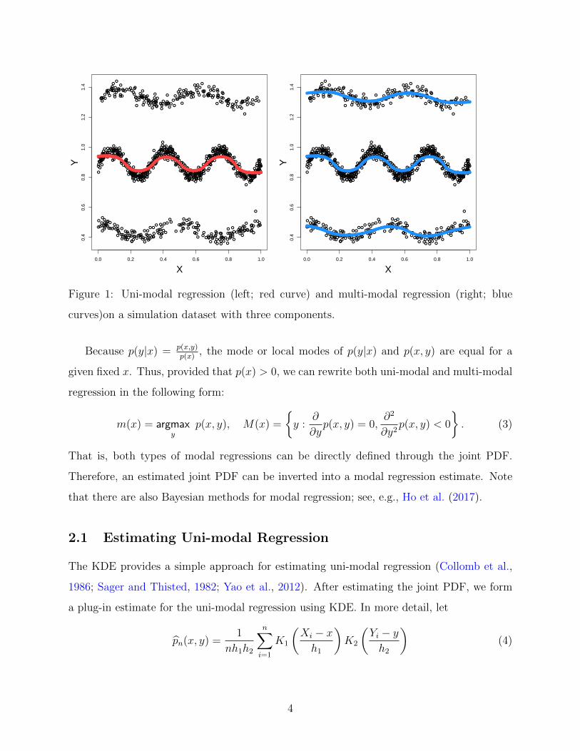
multiple values at a given point x. Figure 1 presents examples of uni-modal and multi-modal

regression using a plug-in estimate from a KDE.

3

●

●

●

●

●

●

●

●●

●

●●

● ●

●

●●

●

●● ●

●●

●●

●

●

●●

●

●

●

●

●●

●●

●

●

●

●

●

●

●

●●

●

●

●

●

●

●

●

●●●

●

●

●

●●

●

●

●

●

●

●

●●

●

●

●

●●

●

●●●

●

●

●

●

●●

●

●●

●

● ●

●

●

●

●

●

●

●

●●●

●●●

●

●

●

●

●●

●

●

●

●

●

●

●●

●●

●

●

●

●

●

●

● ●

●

●●

●

● ●●●

●●

●●

●

●●

● ●● ●

●

●●

● ●●

●

●

●

●

●●

●

●● ●

●● ●

●

●

●●

●

●●

●●

●●●

●

●

●

●

●●

●

●●

●●

● ●

●

●

●

●●

●●

● ●●

●●

●

●

●

●

● ●

●

●

●

●

●●

●

●

●●

●

●

●● ●

●

●

●

●

●

●

● ●

●

●

●

● ●

●

●

●

●

●

●● ●

●●

●

●

●● ●

●

●

●

●

●

●

●

●

●

●●

●

●

●

●

●

●

●

● ●

●●● ●

●

●

●

●

●

●

●

●

● ●

●

●

● ●

●

●● ●

●

●●●

●

●

●

●

●

●

●

●

● ●

●

●

●●

●

●

●

●

●

●

●

●

●

●

●●

●

●

●

●●

●

●

●●

●

●

●

●

●

●

●●

●

●

●

●

● ●

●

●

●●

●

●●

●

●●

●

●

●

●

●●

●

●

●

●

●●

●

●

●

●

●

●

●

●

●●

●

●●

●

●

●

●

●

●

●

●

●

●

●

●

●

●

●

●

●

●

●●

● ●

●

●●

●

●

●

●

●

●

●

●

●

●

● ●● ●

●

●

●

●

●

●

●

●●

● ●●●

●

●

●

●

●●●

●

●

●

●

●●

●

●

●

●

●

● ●

●

●●

●

●

●

●

●

●

●

●

●

●●

●

●

●

●

●

●

●

●

●

●

●

●●

●

●

●

●

●

●

●

●●

●

●

●

●

●●

●

●

●

●

●

●●

●

●

●

●●●

●●

●

●

●

●

●

●

●

●

●

●

●

●●

● ●

●

●

●

●

●

●●

●●

●

●●

●

●

●

●

●●

●●

●

●

●

●

●

●

●

●

●●

●

●●

●●

●●

●

●

●

● ●

●

●

●● ●

●

●●

●

●

● ●

●

●

●●

●

●

●●

●

●

●

●

●

●

●

●

●●

●●

●

●

●

●

●

●

●

●

● ●

●

●

●

●

●

●

●

●

●

●

●

●

●

●

●●●●

●●

●

●●●

●

●

●

●

●

●

●

●

●

●

●

●

●●

●

●●

●

●

●

●

●

●●

●

●●

●

●

●

●●

●

●

●

●

●

●●

●

●

● ●

●

●

●

●

●

●

●

●

●

●

●

●

●

●

●

●

●

●

●

●●

●

●

●●

●

●

●

●

●

●

● ●

●

●

●

●

●

●

●

●

●

●

●

●

●

●

●●

●

● ●

●

●

●

●●●

●

●

●

●●

●●

●

●●

●

●

●

●

●

●●

●

●

●

●●

●

●●●

●

●

●

●

●●

●●

●

●

●

●●

●●

●

●

●

●

●

●●

●

●●

●

● ●

●

●

●

● ●

●

● ●

●

●

●

●

●

●

●●

●

●

●●●●

●

●

●

●

●

●●

●●

●●

●

●

● ●

●●

●●

●

●

●

●●

●

●

● ●

●●

●●

●

●

●●

●

●

●

●●

●●

●

● ●●

●

●

●

●●

●

●

●●

●

●

●

●

●

●

●●

●●

●

●

●

●●

●●●

●

●

●

●

●●

●

●●

● ●

●

●

●● ●

●●

●●

●

●

●●●

●

●●

●

●●

●

●

●

●

●

●●

●

●●

●●

● ●

●●

●●

●●

●●

●

●

●

●

●

●

●

●

●

●

●●

● ●●

●● ●●

●

●

●

●●

●●

●●

●●

●

●

●

●

●

●●

●

●

● ● ●

●

●

●

●●●

●

●

●

●

●

●

●

●●

●

●●

●●

●

0.0 0.2 0.4 0.6 0.8 1.0

0.4

0.6

0.8

1.0

1.2

1.4

X

Y ●●●●●●●●●●●●●●●●●

●●●

●●●●●●●●●●●●●●●●●● ●●

●●●●●●●●●●●●●●●●●●

●●●●●●●●●●●●●●●●●●●●●●●●●●●●●●●●●

●●●●●●●●●●●●●●●●

●●●●●●●●●●●●●●●●

●●●●●●●●●●●●●●●●●

●●●●●●●●●●●●●●●●●●

●●●●●●●●●●●●●

●

●

●

●

●

●

●

●●

●

●●

● ●

●

●●

●

●● ●

●●

●●

●

●

●●

●

●

●

●

●●

●●

●

●

●

●

●

●

●

●●

●

●

●

●

●

●

●

●●●

●

●

●

●●

●

●

●

●

●

●

●●

●

●

●

●●

●

●●●

●

●

●

●

●●

●

●●

●

● ●

●

●

●

●

●

●

●

●●●

●●●

●

●

●

●

●●

●

●

●

●

●

●

●●

●●

●

●

●

●

●

●

● ●

●

●●

●

● ●●●

●●

●●

●

●●

● ●● ●

●

●●

● ●●

●

●

●

●

●●

●

●● ●

●● ●

●

●

●●

●

●●

●●

●●●

●

●

●

●

●●

●

●●

●●

● ●

●

●

●

●●

●●

● ●●

●●

●

●

●

●

● ●

●

●

●

●

●●

●

●

●●

●

●

●● ●

●

●

●

●

●

●

● ●

●

●

●

● ●

●

●

●

●

●

●● ●

●●

●

●

●● ●

●

●

●

●

●

●

●

●

●

●●

●

●

●

●

●

●

●

● ●

●●● ●

●

●

●

●

●

●

●

●

● ●

●

●

● ●

●

●● ●

●

●●●

●

●

●

●

●

●

●

●

● ●

●

●

●●

●

●

●

●

●

●

●

●

●

●

●●

●

●

●

●●

●

●

●●

●

●

●

●

●

●

●●

●

●

●

●

● ●

●

●

●●

●

●●

●

●●

●

●

●

●

●●

●

●

●

●

●●

●

●

●

●

●

●

●

●

●●

●

●●

●

●

●

●

●

●

●

●

●

●

●

●

●

●

●

●

●

●

●●

● ●

●

●●

●

●

●

●

●

●

●

●

●

●

● ●● ●

●

●

●

●

●

●

●

●●

● ●●●

●

●

●

●

●●●

●

●

●

●

●●

●

●

●

●

●

● ●

●

●●

●

●

●

●

●

●

●

●

●

●●

●

●

●

●

●

●

●

●

●

●

●

●●

●

●

●

●

●

●

●

●●

●

●

●

●

●●

●

●

●

●

●

●●

●

●

●

●●●

●●

●

●

●

●

●

●

●

●

●

●

●

●●

● ●

●

●

●

●

●

●●

●●

●

●●

●

●

●

●

●●

●●

●

●

●

●

●

●

●

●

●●

●

●●

●●

●●

●

●

●

● ●

●

●

●● ●

●

●●

●

●

● ●

●

●

●●

●

●

●●

●

●

●

●

●

●

●

●

●●

●●

●

●

●

●

●

●

●

●

● ●

●

●

●

●

●

●

●

●

●

●

●

●

●

●

●●●●

●●

●

●●●

●

●

●

●

●

●

●

●

●

●

●

●

●●

●

●●

●

●

●

●

●

●●

●

●●

●

●

●

●●

●

●

●

●

●

●●

●

●

● ●

●

●

●

●

●

●

●

●

●

●

●

●

●

●

●

●

●

●

●

●●

●

●

●●

●

●

●

●

●

●

● ●

●

●

●

●

●

●

●

●

●

●

●

●

●

●

●●

●

● ●

●

●

●

●●●

●

●

●

●●

●●

●

●●

●

●

●

●

●

●●

●

●

●

●●

●

●●●

●

●

●

●

●●

●●

●

●

●

●●

●●

●

●

●

●

●

●●

●

●●

●

● ●

●

●

●

● ●

●

● ●

●

●

●

●

●

●

●●

●

●

●●●●

●

●

●

●

●

●●

●●

●●

●

●

● ●

●●

●●

●

●

●

●●

●

●

● ●

●●

●●

●

●

●●

●

●

●

●●

●●

●

● ●●

●

●

●

●●

●

●

●●

●

●

●

●

●

●

●●

●●

●

●

●

●●

●●●

●

●

●

●

●●

●

●●

● ●

●

●

●● ●

●●

●●

●

●

●●●

●

●●

●

●●

●

●

●

●

●

●●

●

●●

●●

● ●

●●

●●

●●

●●

●

●

●

●

●

●

●

●

●

●

●●

● ●●

●● ●●

●

●

●

●●

●●

●●

●●

●

●

●

●

●

●●

●

●

● ● ●

●

●

●

●●●

●

●

●

●

●

●

●

●●

●

●●

●●

●

0.0 0.2 0.4 0.6 0.8 1.0

0.4

0.6

0.8

1.0

1.2

1.4

XY

●●●●●●●●●●●●●●●●●●●●●●●●●●●●●●●●●●●●●●●●●●●●●●●●●●●●●●●●●●●●●●●●●●●●●●●●●●●●●●●●●●●●●●●●●●●●●●●●●●●●●●●●●●●●●●●●●●●●

●●●●●●●●●●●●●●●●●

●●●

●●●●●●●●●●●●●●●●●●

●●●●●●●●●●●●●●●●●●

●●●●●●●●

●●●●●●●●●●●●●●●●●●●●

●●●●●●●●●●●●●●●●●●●●●●●●●●●●●●●●●

●●●●●●●●●●●●●●●●

●●●●●●●●●●●●●●●●

●●●●●●●●●●●●●●●●●

●●●●●●●●●●●●●●●●●●

●●●●●●●●●●●●●

●●●●●●●●●●●●●●●●●●●●●●●●●●●●●●●●●●●●●●●●●●●●●●●●●●●●●●●●●●●●●●●●●●●●●●●●●●●●●●●●●●●●●●●

●●●●●●●●●●●●●●●●●●●●●●●●●●●●●●●●●●●●●●●●●●●●●●●●●●●●●●●●●●●●●●●●●●●●●●●●●●●●●●●●●●●●●●●●●●●●●●●●●●●●

Figure 1: Uni-modal regression (left; red curve) and multi-modal regression (right; blue

curves)on a simulation dataset with three components.

Because p(y|x) = p(x,y)p(x)

, the mode or local modes of p(y|x) and p(x, y) are equal for a

given fixed x. Thus, provided that p(x) > 0, we can rewrite both uni-modal and multi-modal

regression in the following form:

m(x) = argmaxy

p(x, y), M(x) =

{y :

∂

∂yp(x, y) = 0,

∂2

∂y2p(x, y) < 0

}. (3)

That is, both types of modal regressions can be directly defined through the joint PDF.

Therefore, an estimated joint PDF can be inverted into a modal regression estimate. Note

that there are also Bayesian methods for modal regression; see, e.g., Ho et al. (2017).

2.1 Estimating Uni-modal Regression

The KDE provides a simple approach for estimating uni-modal regression (Collomb et al.,

1986; Sager and Thisted, 1982; Yao et al., 2012). After estimating the joint PDF, we form

a plug-in estimate for the uni-modal regression using KDE. In more detail, let

pn(x, y) =1

nh1h2

n∑i=1

K1

(Xi − xh1

)K2

(Yi − yh2

)(4)

4

be the KDE where K1 and K2 are kernel functions such as Gaussian functions and h1, h2 > 0

are smoothing parameters that control the amount of smoothing. An estimator of m is

mn(x) = argmaxy

pn(x, y). (5)

Note that the joint PDF can be estimated by other approaches such as local polynomial

estimation as well (Einbeck and Tutz, 2006; Fan et al., 1996; Fan and Yim, 2004).

Equation (4) has been generalized to the case of censored response variables. Khardani

et al. (2010, 2011); Ould-Saıd and Cai (2005). Suppose that instead of observing the response

variables Y1, · · · , Yn, we observe Ti = min{Yi, Ci} and an indicator δi = I(Ti = Yi) that

informs whether Yi is observed or not and Ci is an random variable that is independent of

Xi and Yi. In this case, equation (4) can be modified to

p†n(x, y) =1

nh1h2

n∑i=1

K1

(Xi − xh1

)K2

(Ti − yh2

)× δi

Sn(Ti), (6)

where Sn(t) is the Kaplan-Meier estimator (Kaplan and Meier, 1958)

Sn(t) =

∏n

i=1

(1− δ(i)

n−i+1

)I(T(i)≤t)if t < T(n),

0 otherwise,

with T(1) ≤ T(2) ≤ · · · ≤ T(n) being the ordered Ti’s and δ(i) being the value of δ for the i-th

ordered observation. Replacing pn by p†n in equation (5), we obtain a uni-modal regression

estimator in the censoring case.

Uni-modal regression may be estimated parametrically as well. When K2 is a spherical

(box) kernel K2(x) = 12I(|x| ≤ 1), the argmax operation is equivalent to the argmin opeartor

on a flattened 0 − 1 loss. In more detail, consider a 1D toy example with observations

Z1, · · · , Zn and a corresponding KDE q(z) = 12nh

∑ni=1 I(|z − Zi| ≤ h) obtained with a

spherical kernel. It is easily seen that

argmaxz

q(z) = argmaxz

1

2nh

n∑i=1

I(|z − Zi| ≤ h)

= argmaxz

n∑i=1

I(|z − Zi| ≤ h)

= argminz

n∑i=1

I(|z − Zi| > h).

(7)

5

Parametric uni-modal regression forms estimators using equation (7) or its generalizations

(Kemp and Silva, 2012; Khardani and Yao, 2017; Krief, 2017; Lee, 1989, 1993; Lee and Kim,

1998; Manski, 1991; Yao and Li, 2014). Parameters estimated through the maximizing crite-

rion in equation (7) is equivalent to maximum likelihood estimation. Conversely, parameter

estimation through the minimization procedure in equation (7) is equivalent to empirical

risk minimization. For example, to fit a linear model to m(x) = β0 + β1x (Lee, 1989; Yao

and Li, 2014), we can use the fitted parameters

β0, β1 = argmaxβ0,β1

1

2nh

n∑i=1

I(|β0 + β1Xi − Yi| ≤ h)

= argminβ0,β1

n∑i=1

I(|β0 + β1Xi − Yi| > h)

(8)

to construct our final estimate of m(x).

Using equation (7), we can always convert the problem of finding the uni-modal regression

into a problem of minimizing a loss function. Here, the tuning parameter h can be interpreted

as the smoothing bandwidth of the applied spherical kernel. Choosing h is a persistently

difficult task. Some possible approaches will be discussed in Section 4.

2.2 Estimating Multi-modal Regression

Like uni-modal regression, multi-modal regression can be estimated using a plug-in estimate

from the KDE (Chen et al., 2016a; Einbeck and Tutz, 2006). Recalling that pn(x, y) is the

KDE of the joint PDF, an estimator of M(x) is

Mn(x) =

{y :

∂

∂ypn(x, y) = 0,

∂2

∂y2pn(x, y) < 0

}. (9)

Namely, we use the conditional local modes of the KDE to estimate the conditional local

modes of the joint PDF. Plug-ins from a KDE have been applied in estimations of many

structures (Chen, 2017; Scott, 2015) such as the regression function(Nadaraya, 1964; Watson,

1964), modes (Chacon and Duong, 2013; Chen et al., 2016b), ridges (Chen et al., 2016a;

Genovese et al., 2014), and level sets (Chen et al., 2017a; Rinaldo and Wasserman, 2010).

An alternative way of estimating the multi-modal regression was proposed in Sasaki et al.

(2016).

6

In the measurement error case where the covariates X1, · · · , Xn are observed with noises,

we can replace K1 by a deconvolution kernel to obtain a consistent estimator (Zhou and

Huang, 2016). In more detail, let

Wi = Xi + Ui, i = 1, · · · , n,

where U1, · · · , Un are IID measurement errors that are independent of the covariates and

responses. We assume that the PDF of U1, fU(u), is known. Here we observe not Xi’s but

pairs of (W1, Y1), · · · , (Wn, Yn). Namely, we observe the response variable and its corrupted

covariate. In this case, (4) is replaced by

pn(x, y) =1

nh1h2

n∑i=1

KU

(Wi − xh1

)K2

(Yi − yh2

), (10)

where

KU(t) =1

2π

∫e−its

φK1(s)

φU(s/h1)ds

with φK1 and φU being the Fourier transforms of K1 and fU , respectively. The estimator of

M then becomes the conditional local modes of p:

Mn(x) =

{y :

∂

∂ypn(x, y) = 0,

∂2

∂y2pn(x, y) < 0

}(11)

For more details, the reader is referred to Zhou and Huang (2016).

2.3 Uni-modal versus Multi-modal Regression

Uni-modal and multi-modal regression have their own advantages and disadvantages. Uni-

modal regression is an alternative approach for summarizing the covariate-response relation-

ship using a single function. Multi-modal regression performs a similar job but allows a

multi-valued summary function. When the relation between the response and the covariate

is complicated or has several distinct components (see, e.g., Figure 1), multi-modal regression

may detect the hidden relation that cannot be found by uni-modal regression. In particu-

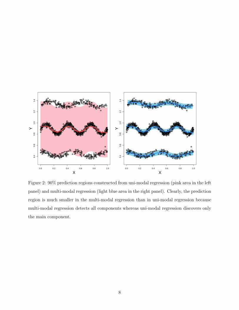
lar, the prediction regions tend to be smaller in multi-modal regression than in uni-modal

regression (see Figure 2 for an example). However, multi-modal regression often returns a

multi-valued function that is more difficult to interpret than the output from a uni-modal

regression.

7

0.0 0.2 0.4 0.6 0.8 1.0

0.4

0.6

0.8

1.0

1.2

1.4

X

Y

●

●

●

●

●

●

●

● ●

●

●●

● ●

●

●●

●

●● ● ●

●

●●

●

●

●●

●

●

●

●

●●

●●

●

●

●

●

●

●

●

●●

●

●

●

●

●

●

●

●●●

●

●

●

● ●●

●

●

●

●

●

●●

●●

●

●●

●

●●●

●

●

●

●

●●●

●●

●

● ●

●

●

●

●

●

●

●

●●●

●●●

●

●

●

●

●●

●

●

●

●

●

●

● ●

●●

●

●

●

●

●

●

● ●

●

●●

●

● ●●●

●●

●●

●

●●

● ●● ●

●

●●

● ●●

●

●

●●

●●

●

●● ●

●● ●

●

●●

●

●

●●

●●

●●●

●

●

●

●

●●

●

●●

●●

● ●

●

●

●

●●

●●

● ●●

●●

●

●

●

●

● ●

●

●

●

●

●●

●

●

●●

●

●

●● ●

●

●

●

●

●

●

● ●

●

●

●

● ●

●

●

●

●

●

●● ●

●●

●

●

●● ●

●

●

●

●

●

●

●

●

●

●●

●

●

●

●

●

●

●

● ●

●●● ●

●

●

●

●

●

●

●

●

● ●

●

●

● ●

●

●● ●

●

●●●

●

●

●

●

●

●

●

●

● ●

●

●

●●

●

●

●

●

●

●

●

●

●

●

●●

●

●

●

●●

●

●

●●●

●

●

●

●

●

●●

●

●

●

●

● ●

●

●

●●

●

●●

●

●●

●

●

●

●

●●

●

●

●

●

●●

●

●

●

●

●

●

●

●

●●

●

●●

●

●

●

●

●

●

●

●

●

●

●

●

●

●

●

●

●

●

●●

● ●

●

●●

●

●

●●

●

●

●

●

●

●

● ●● ●

●

●

●

●

●

●

●

●●

● ●●●

●

●

●

●

●●●

●

●

●

●

●●

●

●

●

●

●● ●

●

●●

●

●

●

●

●

●

●

●

●

●●

●

●

●

●

●

●

●

●

●

●

●

●●

●

●

●

●

●

●

●

●●

●

●

●

●

●●

●

●

●

●

●

●●

●

●

●

●●●

●●

●

●

●

●

●

●

●

●

●

●

●

●●

● ●

●

●

●

●

●

●●

●●

●

●●

●

●

●

●

●●

●●

●●

●

●

●

●

●

●

●●

●●

●

●●

●●

●

●

●

● ●

●

●

●● ●

●

●●

●

●

● ●

●

●

●●

●

●●

●

●

●

●

●

●

●

●

●

●●

●●

●

●

●

●

●

●

●

●

● ●

●●

●

●

●

●

●

●

●

●

●

●

●

●

●●●●

●●

●

●●●

●

●

●

●

●

●

●

●

●

●

●

●

●●

●

●●

●●

●

●

●

●●

●

●●

●

●

●

●●

●

●

●

●

●

●●

●

●

● ●

●

●

●

●

●

●

●

●

●

●

●

●

●

●

●●

●

●

●

●●

●

●

●●

●

●

●

●

●

●

● ●

●

●

●

●

●

●

●

●●

●

●

●

●●

●●

●

● ●

●

●

●

●●●

●

●

●

●●

●●

●

●●

●

●

●

●

●

●●

●

●

●

● ●

●

●●●

●

●

●

●

●●

●●

●

●

●

●●

●●

●

●

●

●

●

●●

●

●●

●

● ●

●

●

●

● ●

●

● ●

●

●

●

●

●

●

●●

●

●

●●●●

●

●

●

●

●

●●

●●

●●

●

●

● ●

● ●

●●

●

●

●

●●

●

●

● ●

●●

●●

●

●

●●

●

●

●

●●●

●●

● ● ●

●

●

●

●●

●

●

●●

●

●

●

●

●

●

●●

●●

●

●

●

●●

●●●

●

●

●

●

●●

●

●●

● ●

●

●

●● ●

●●

●●

●

●

●●●

●

●●

●

●●

●

●

●

●

●

●●

●

●●

●●

● ●

●●

●●

●●

●●

●

●

●

●

●

●●

●

●

●

●●

● ●●

● ● ●●●

●

●

●●

●●

●●

●●

●

●

●

●

●

●●

●

●

● ● ●

●

●

●

●●●

●●

●

●

●

●●

●●

●

●●

●●

●

0.0 0.2 0.4 0.6 0.8 1.0

0.4

0.6

0.8

1.0

1.2

1.4

X

Y

●

●

●

●

●

●

●

● ●

●

●●

● ●

●

●●

●

●● ● ●

●

●●

●

●

●●

●

●

●

●

●●

●●

●

●

●

●

●

●

●

●●

●

●

●

●

●

●

●

●●●

●

●

●

● ●●

●

●

●

●

●

●●

●●

●

●●

●

●●●

●

●

●

●

●●●

●●

●

● ●

●

●

●

●

●

●

●

●●●

●●●

●

●

●

●

●●

●

●

●

●

●

●

● ●

●●

●

●

●

●

●

●

● ●

●

●●

●

● ●●●

●●

●●

●

●●

● ●● ●

●

●●

● ●●

●

●

●●

●●

●

●● ●

●● ●

●

●●

●

●

●●

●●

●●●

●

●

●

●

●●

●

●●

●●

● ●

●

●

●

●●

●●

● ●●

●●

●

●

●

●

● ●

●

●

●

●

●●

●

●

●●

●

●

●● ●

●

●

●

●

●

●

● ●

●

●

●

● ●

●

●

●

●

●

●● ●

●●

●

●

●● ●

●

●

●

●

●

●

●

●

●

●●

●

●

●

●

●

●

●

● ●

●●● ●

●

●

●

●

●

●

●

●

● ●

●

●

● ●

●

●● ●

●

●●●

●

●

●

●

●

●

●

●

● ●

●

●

●●

●

●

●

●

●

●

●

●

●

●

●●

●

●

●

●●

●

●

●●●

●

●

●

●

●

●●

●

●

●

●

● ●

●

●

●●

●

●●

●

●●

●

●

●

●

●●

●

●

●

●

●●

●

●

●

●

●

●

●

●

●●

●

●●

●

●

●

●

●

●

●

●

●

●

●

●

●

●

●

●

●

●

●●

● ●

●

●●

●

●

●●

●

●

●

●

●

●

● ●● ●

●

●

●

●

●

●

●

●●

● ●●●

●

●

●

●

●●●

●

●

●

●

●●

●

●

●

●

●● ●

●

●●

●

●

●

●

●

●

●

●

●

●●

●

●

●

●

●

●

●

●

●

●

●

●●

●

●

●

●

●

●

●

●●

●

●

●

●

●●

●

●

●

●

●

●●

●

●

●

●●●

●●

●

●

●

●

●

●

●

●

●

●

●

●●

● ●

●

●

●

●

●

●●

●●

●

●●

●

●

●

●

●●

●●

●●

●

●

●

●

●

●

●●

●●

●

●●

●●

●

●

●

● ●

●

●

●● ●

●

●●

●

●

● ●

●

●

●●

●

●●

●

●

●

●

●

●

●

●

●

●●

●●

●

●

●

●

●

●

●

●

● ●

●●

●

●

●

●

●

●

●

●

●

●

●

●

●●●●

●●

●

●●●

●

●

●

●

●

●

●

●

●

●

●

●

●●

●

●●

●●

●

●

●

●●

●

●●

●

●

●

●●

●

●

●

●

●

●●

●

●

● ●

●

●

●

●

●

●

●

●

●

●

●

●

●

●

●●

●

●

●

●●

●

●

●●

●

●

●

●

●

●

● ●

●

●

●

●

●

●

●

●●

●

●

●

●●

●●

●

● ●

●

●

●

●●●

●

●

●

●●

●●

●

●●

●

●

●

●

●

●●

●

●

●

● ●

●

●●●

●

●

●

●

●●

●●

●

●

●

●●

●●

●

●

●

●

●

●●

●

●●

●

● ●

●

●

●

● ●

●

● ●

●

●

●

●

●

●

●●

●

●

●●●●

●

●

●

●

●

●●

●●

●●

●

●

● ●

● ●

●●

●

●

●

●●

●

●

● ●

●●

●●

●

●

●●

●

●

●

●●●

●●

● ● ●

●

●

●

●●

●

●

●●

●

●

●

●

●

●

●●

●●

●

●

●

●●

●●●

●

●

●

●

●●

●

●●

● ●

●

●

●● ●

●●

●●

●

●

●●●

●

●●

●

●●

●

●

●

●

●

●●

●

●●

●●

● ●

●●

●●

●●

●●

●

●

●

●

●

●●

●

●

●

●●

● ●●

● ● ●●●

●

●

●●

●●

●●

●●

●

●

●

●

●

●●

●

●

● ● ●

●

●

●

●●●

●●

●

●

●

●●

●●

●

●●

●●

●

Figure 2: 90% prediction regions constructed from uni-modal regression (pink area in the left

panel) and multi-modal regression (light blue area in the right panel). Clearly, the prediction

region is much smaller in the multi-modal regression than in uni-modal regression because

multi-modal regression detects all components whereas uni-modal regression discovers only

the main component.

8

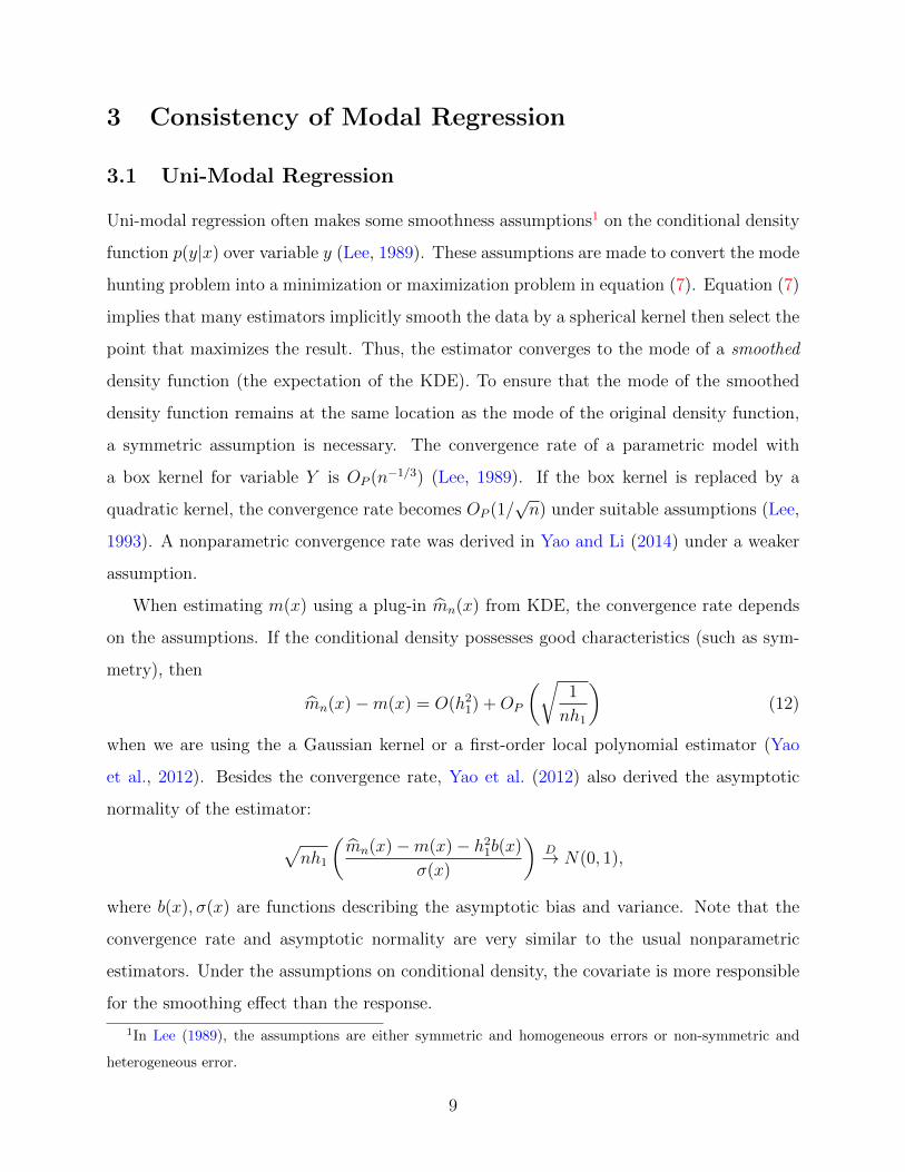
3 Consistency of Modal Regression

3.1 Uni-Modal Regression

Uni-modal regression often makes some smoothness assumptions1 on the conditional density

function p(y|x) over variable y (Lee, 1989). These assumptions are made to convert the mode

hunting problem into a minimization or maximization problem in equation (7). Equation (7)

implies that many estimators implicitly smooth the data by a spherical kernel then select the

point that maximizes the result. Thus, the estimator converges to the mode of a smoothed

density function (the expectation of the KDE). To ensure that the mode of the smoothed

density function remains at the same location as the mode of the original density function,

a symmetric assumption is necessary. The convergence rate of a parametric model with

a box kernel for variable Y is OP (n−1/3) (Lee, 1989). If the box kernel is replaced by a

quadratic kernel, the convergence rate becomes OP (1/√n) under suitable assumptions (Lee,

1993). A nonparametric convergence rate was derived in Yao and Li (2014) under a weaker

assumption.

When estimating m(x) using a plug-in mn(x) from KDE, the convergence rate depends

on the assumptions. If the conditional density possesses good characteristics (such as sym-

metry), then

mn(x)−m(x) = O(h21) +OP

(√1

nh1

)(12)

when we are using the a Gaussian kernel or a first-order local polynomial estimator (Yao

et al., 2012). Besides the convergence rate, Yao et al. (2012) also derived the asymptotic

normality of the estimator:√nh1

(mn(x)−m(x)− h21b(x)

σ(x)

)D→ N(0, 1),

where b(x), σ(x) are functions describing the asymptotic bias and variance. Note that the

convergence rate and asymptotic normality are very similar to the usual nonparametric

estimators. Under the assumptions on conditional density, the covariate is more responsible

for the smoothing effect than the response.

1In Lee (1989), the assumptions are either symmetric and homogeneous errors or non-symmetric and

heterogeneous error.

9

Various studies have reported the convergence of uni-modal regression with dependent

covariates (Attaoui, 2014; Collomb et al., 1986; Dabo-Niang and Laksaci, 2010; Khardani

et al., 2010, 2011; Ould-Saıd, 1993, 1997; Ould-Saıd and Cai, 2005). Strong consistency was

investigated in (Collomb et al., 1986; Ould-Saıd, 1993, 1997). The convergence rate has also

been derived in uni-modal regression with functional dependent covariates Attaoui (2014);

Dabo-Niang and Laksaci (2010), and with censored response Khardani et al. (2010, 2011);

Ould-Saıd and Cai (2005).

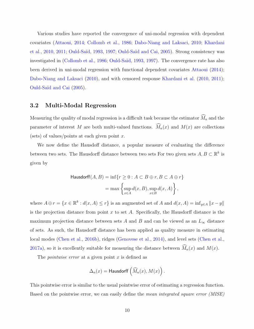
3.2 Multi-Modal Regression

Measuring the quality of modal regression is a difficult task because the estimator Mn and the

parameter of interest M are both multi-valued functions. Mn(x) and M(x) are collections

(sets) of values/points at each given point x.

We now define the Hausdoff distance, a popular measure of evaluating the difference

between two sets. The Hausdorff distance between two sets For two given sets A,B ⊂ Rk is

given by

Hausdorff(A,B) = inf{r ≥ 0 : A ⊂ B ⊕ r, B ⊂ A⊕ r}

= max

{supx∈A

d(x,B), supx∈B

d(x,A)

},

where A⊕ r = {x ∈ Rk : d(x,A) ≤ r} is an augmented set of A and d(x,A) = infy∈A ‖x− y‖

is the projection distance from point x to set A. Specifically, the Hausdorff distance is the

maximum projection distance between sets A and B and can be viewed as an L∞ distance

of sets. As such, the Hausdorff distance has been applied as quality measure in estimating

local modes (Chen et al., 2016b), ridges (Genovese et al., 2014), and level sets (Chen et al.,

2017a), so it is excellently suitable for measuring the distance between Mn(x) and M(x).

The pointwise error at a given point x is defined as

∆n(x) = Hausdorff(Mn(x),M(x)

).

This pointwise error is similar to the usual pointwise error of estimating a regression function.

Based on the pointwise error, we can easily define the mean integrated square error (MISE)

10

and uniform errors

MISEn =

∫∆2n(x)dx, ∆n = sup

x∆n(x).

These quantities are generalized from the errors in nonparametric literature (Scott, 2015).

The convergence rate of Mn(x) has been derived in Chen et al. (2016a):

∆n(x) = O(h21 + h22) +OP

(√1

nh1h32

)

∆n = O(h21 + h22) +OP

(√log n

nh1h32

)

MISEn = O(h41 + h42) +O

(log n

nh1h32

).

(13)

The bias is now contributed by smoothing covariates and response. The convergence rate

of the stochastic variation, OP

(√1

nh1h32

), depends on the amount of smoothing in both the

covariate and response variable as well. The component h32 can be decomposed as h2 · h22,

where the first part h2 is the usual smoothing and the second part, h22, is from derivative

estimations. Note that the convergence rates in equation (13) require no symmetric-like

assumption on the conditional density, but only smoothness and bounded curvature at each

local mode. Therefore, the assumptions ensuring a consistent estimator are much weaker in

multi-modal regression than in uni-modal regression. However, the convergence rate is much

slower in multi-modal regression than in uni-modal regression (equation (12)). Note that

under the same weak assumptions as multi-modal regression, uni-modal regression can also

be consistently estimated by a KDE and the convergence rate will be the same as equation

(13).

Chen et al. (2016a) also derived the asymptotic distribution and a bootstrap theory of ∆n.

When we ignore the bias, the uniform error converges to the maximum of a Gaussian process

and the distribution of this a maximum can be approximated by the empirical bootstrap

(Efron, 1979). Therefore, by applying the bootstrap, one can construct a confidence band

for the modal regression.

In the case of measurement errors, a similar convergence rate to equation (13) can also

be derived under suitable conditions (Zhou and Huang, 2016). Note that in this case, the

distribution of measurement errors also affects the estimation quality.

11

4 Bandwidth Selection

Modal regression estimation often involves some tuning parameters. In a parametric model,

we have to choose a window size h in equation (7). In other models, we often require two

smoothing bandwidths: one for the response variable, the other for the covariate. Here we

briefly summarize some bandwidth selectors proposed in the literature.

4.1 Plug-in Estimate

In Yao et al. (2012), uni-modal regression was estimated by a local polynomial estimator.

One advantage of uni-modal regression is the closed-form expression of the first-order error.

Therefore, we can use a plug-in approach to obtain an initial error estimate and convert it

into a possible smoothing bandwidth. This approach is very similar to the plug-in bandwidth

selection in the density estimation problem (Sheather, 2004).

This approach was designed to optimally estimating the error of a uni-modal regression

estimate. However, this method is often not applicable to multi-modal regression because a

closed-form expression of the first-order error is often unavailable. Moreover, this approach

requires a pilot estimate for the first error. If the pilot estimate is unreliable, the performance

of the bandwidth selector may be seriously compromised.

4.2 Adapting from Conditional Density Estimation

A common approach for selecting the tuning parameter is based on optimizing the estimation

accuracy of conditional density function (Fan et al., 1996; Fan and Yim, 2004). For instance,

the authors of Einbeck and Tutz (2006) adapted the smoothing bandwidth to multi-modal

regression by optimizing the conditional density estimation rate and the Silverman’s normal

reference rule (Silverman, 1986).

The principle of adapting from estimating the conditional density often relies on opti-

12

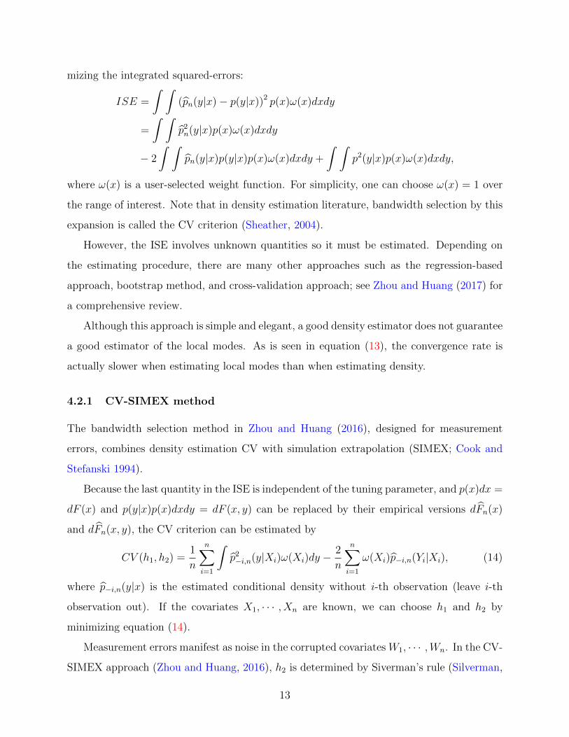
mizing the integrated squared-errors:

ISE =

∫ ∫(pn(y|x)− p(y|x))2 p(x)ω(x)dxdy

=

∫ ∫p2n(y|x)p(x)ω(x)dxdy

− 2

∫ ∫pn(y|x)p(y|x)p(x)ω(x)dxdy +

∫ ∫p2(y|x)p(x)ω(x)dxdy,

where ω(x) is a user-selected weight function. For simplicity, one can choose ω(x) = 1 over

the range of interest. Note that in density estimation literature, bandwidth selection by this

expansion is called the CV criterion (Sheather, 2004).

However, the ISE involves unknown quantities so it must be estimated. Depending on

the estimating procedure, there are many other approaches such as the regression-based

approach, bootstrap method, and cross-validation approach; see Zhou and Huang (2017) for

a comprehensive review.

Although this approach is simple and elegant, a good density estimator does not guarantee

a good estimator of the local modes. As is seen in equation (13), the convergence rate is

actually slower when estimating local modes than when estimating density.

4.2.1 CV-SIMEX method

The bandwidth selection method in Zhou and Huang (2016), designed for measurement

errors, combines density estimation CV with simulation extrapolation (SIMEX; Cook and

Stefanski 1994).

Because the last quantity in the ISE is independent of the tuning parameter, and p(x)dx =

dF (x) and p(y|x)p(x)dxdy = dF (x, y) can be replaced by their empirical versions dFn(x)

and dFn(x, y), the CV criterion can be estimated by

CV (h1, h2) =1

n

n∑i=1

∫p2−i,n(y|Xi)ω(Xi)dy −

2

n

n∑i=1

ω(Xi)p−i,n(Yi|Xi), (14)

where p−i,n(y|x) is the estimated conditional density without i-th observation (leave i-th

observation out). If the covariates X1, · · · , Xn are known, we can choose h1 and h2 by

minimizing equation (14).

Measurement errors manifest as noise in the corrupted covariates W1, · · · ,Wn. In the CV-

SIMEX approach (Zhou and Huang, 2016), h2 is determined by Siverman’s rule (Silverman,

13

1986) and we give a brief summary for the selection of h1 as follows. We first generate

W ∗1 , · · · ,W ∗

n where W ∗i = Wi + U∗i and U∗1 , · · · , U∗n are IID from the measurement error

distribution. Then we construct the estimator p∗n by replacing X1, · · · , Xn by W ∗1 , · · · ,W ∗

n .

We modify equation (14) by replacing X1, · · · , Xn by W1, · · · ,Wn and replacing pn by p∗n

Note that the weight ω will also be updated according to the range of W ’s. Let CV ∗(h1) be

the resulting CV criterion. Now we compute another CV criterion as follows. We generate

W ∗∗1 , · · · ,W ∗∗

n where W ∗∗i = W ∗

i + U∗∗i and U∗∗1 , · · · , U∗∗n are IID from the measurement

error distribution. Similar to the previous steps, we compute a new (conditional) density

estimator p∗∗n by replacing X1, · · · , Xn by W ∗∗1 , · · · ,W ∗∗

n . To obtain a new CV criterion, we

again modify equation (14) by replacing X1, · · · , Xn by W ∗1 , · · · ,W ∗

n and replacing pn by

p∗∗n . This leads to a new CV criterion which we denoted as CV ∗∗(h1). We then repeat the

above process multiple times and calculate the average CV∗(h1) and CV

∗∗(h1). Then we

choose h∗1 to be the minimizer of CV∗(h1) and h∗∗1 to be the minimizer of CV

∗∗(h1). The

final choice of smoothing bandwidth is h1 =h∗21h∗∗1

.

The CV procedure assesses the quality of estimating the conditional density. The simu-

lation process (SIMEX part) exploits the similarity between the optimal h1–h∗1 relation and

the h∗1–h∗∗1 relation, i.e., h1,opt

h∗1≈ h∗1

h∗∗1. Thus, the smoothing bandwidth is selected by equating

this approximation.

However, CV-SIMEX optimizes the quality of estimating the conditional density, not the

conditional local modes. As confirmed in equation (13), the optimal convergence rate differs

between density and local modes estimation, so this choice would undersmooth the local

modes estimation.

4.2.2 Modal CV-criteria

Zhou and Huang (2017) proposed a generalization of the density estimation CV criterion to

the multi-modal regression. The idea is to replace the ISE by

ISEM =

∫Hausdorff2

(Mn(x),M(x)

)p(x)ω(x)dx

and find an estimator of the above quantity. Optimizing the corresponding estimated ISEM

leads to a good rule for selecting the smoothing bandwidth. In particular, Zhou and Huang

14

(2017) proposed to use a bootstrap approach to estimate ISEM . The quantity ISEM is

directly tailored to the modal regression rather than conditional density estimation so it

reflects the actual accuracy of modal regression.

4.3 Prediction Band Approach

Another bandwidth selector for multi-modal regression was proposed in Chen et al. (2016a).

This approach optimizes the size of the prediction bands using a cross-validation (CV) in

the regression analysis. After selecting a prediction level (e.g., 95%), the data is split into

a training set and a validation set. The modal regression estimator is constructed from

the data in the training set, and the residuals of the observations are derived from the

validation set. The residual of a pair Xval, Yval is based on the shortest distance to the

nearly conditional local mode. Namely, the residual for an observation (Xval, Yval) in the

validation set is eval = miny∈Mn(Xval)‖Yval − y‖. The 95% quantile of the residuals specifies

the radius of a 95% prediction band. The width of a prediction band is twice the estimated

radius. After repeating this procedure several times as the usual CV, we obtain an average

size (volume of the prediction band) of the prediction band of each smoothing bandwidth.

The smoothing bandwidth is chosen to be the one that has the smallest (in terms of volume)

prediction band.

When h is excessively small, there will be many conditional local modes which leads to

a large prediction band. On the other hand, when h is too large, the number of conditional

local modes are small but each of them has a very large band, yielding a large total size of

the prediction band. Consequently, this approach leads to a stable result.

However, the prediction band approach is beset with several problems. First, the optimal

choice of smoothing bandwidth depends on the prediction level, which cannot be definitely

selected at present. Second, calculating the size of a band is computationally challenging

in high dimensions. Third, there is no theoretical guarantee that the selected bandwidth

follows the optimal convergence rate.

Note that Zhou and Huang (2017) proposed a modified CV criterion for approximating

the size of prediction band without specifying the prediction level. This approach avoids the

problem of selecting a prediction level and is computationally more feasible.

15

5 Computational Methods

In the modal regression estimation, a closed-form solution to the estimator is often unavail-

able. Therefore, the estimator must be computed by a numerical approach. The parameters

in uni-modal regression with a parametric model can be estimated by a mode-hunting pro-

cedure (Lee, 1989). When estimating uni-modal regression by a nonparametric approach,

the conditional mode can be found by the gradient ascent method or an EM-algorithm (Yao

and Li, 2014; Yao et al., 2012).

The conditional local modes in multi-modal regression can also be found by a gradient

ascent approach. If the kerne function of the response variable K2 has a nice form such

as being a Gaussian function, gradient ascent can be easily performed by a simple algo-

rithm called meanshift algorithm (Cheng, 1995; Comaniciu and Meer, 2002; Fukunaga and

Hostetler, 1975). In the following, we briefly review the EM algorithm and the meanshift

algorithm for finding modes and explain their applications to modal regression.

5.1 EM Algorithm

A common approach for finding uni-modal regression is the EM algorithm (Dempster et al.,

1977; Wu, 1983). In the case of modal regression, we use the idea from a modified method

called the modal EM algorithm (Li et al., 2007; Yao et al., 2012). For simplicity, we illustrate

the EM algorithm using the linear uni-modal regression problem with a single covariate (Yao

and Li, 2014). Let (X1, Y1), · · · , (Xn, Yn) be the observed data and recall that the uni-modal

regression finds the parameters using

β0, β1 = argmaxβ0,β1

1

nh

n∑i=1

K

(Yi − β0 − β1Xi

h

). (15)

Note that when we take K(x) = K2(x) = 12I(|x| ≤ 1), we obtain equation (8).

Given an initial choice of parameters β(0)0 , β

(0)1 , the EM algorithm iterates the following

two steps until convergence (t = 1, 2, · · · ):

16

• E-step. Given β(t−1)0 , β

(t−1)1 , compute the weights

π(i|β(t−1)

0 , β(t−1)1

)=

K

(Yi−β

(t−1)0 −β(t−1)

1 Xi

h

)∑n

j=1K

(Yj−β

(t−1)0 −β(t−1)

1 Xj

h

)for each i = 1, · · · , n.

• M-step. Given the weights, update the parameters by

β(t)0 , β

(t)1 = argmax

β0,β1

1

n

n∑i=1

π(i|β(t−1)0 , β

(t−1)1 ) logK

(Yi − β0 − β1Xi

h

).

When the kernel function K is a Gaussian, the M-step has a closed-form expression:

β(t)0 , β

(t)1 = (XTW(t)XT )−1XTW(t)Y,

where XT = ((1, X1)T , (1, X2)

T , · · · , (1, Xn)T ) is the transpose of the covariate matrix in

regression problem and W(t) is an n× n diagonal matrix with elements

π(1|β(t−1)0 , β

(t−1)1 ), · · · , π(n|β(t−1)

0 , β(t−1)1 )

and Y = (Y1, · · · , Yn)T is the response vector. This is because the problem reduces to a

weighted least square estimator in linear regression. Thus, the updates can be done very

quickly.

Note that the EM algorithm may stuck at the local optima (Yao and Li, 2014) so the

choice of initial parameters is very important. In practice, we would recommend to rerun

the EM algorithm with many different initial parameters to avoid the problem of falling in

a local maximum.

The EM algorithm can be extended to nonparametric uni-modal regression as well. See

Yao et al. (2012) for an example of applying the EM algorithm to find the uni-modal regres-

sion using a local polynomial estimator.

5.2 Meanshift Algorithm

To illustrate the principle of the meanshift algorithm (Cheng, 1995; Comaniciu and Meer,

2002; Fukunaga and Hostetler, 1975), we return to the 1D toy example. Suppose that we

17

observe IID random samples Z1, · · · , Zn ∼ q. Let q be a KDE with a Gaussian kernel

KG(x) = 1√2πe−x

2/2. A powerful feature of the Gaussian kernel is that its nicely behave

derivative:

K ′G(x) = −x · 1√2πe−x

2/2 = −x ·KG(x).

The derivative of the KDE is then

q′(z) =d

dz

1

nh

n∑i=1

KG

(Zi − zh

)=

1

nh3

n∑i=1

(Zi − z)KG

(Zi − zh

)=

1

nh3

n∑i=1

ZiKG

(Zi − zh

)− z

nh3

n∑i=1

KG

(Zi − zh

).

Multiplying both sides by nh3 and dividing them by∑n

i=1KG

(Zi−zh

), the above equation

becomesnh3∑n

i=1KG

(Zi−zh

) · q′(z) =

∑ni=1 ZiKG

(Zi−zh

)∑ni=1KG

(Zi−zh

) − z.Rearranging this expression, we obtain

z︸︷︷︸current location

+nh3∑n

i=1KG

(Zi−zh

) · q′(z)︸ ︷︷ ︸gradient aescent

=

∑ni=1 ZiKG

(Zi−zh

)∑ni=1KG

(Zi−zh

)︸ ︷︷ ︸next location

Namely, given a point z, the value of∑n

i=1 ZiKG(Zi−z

h )∑ni=1KG(Zi−z

h )is a shifted location by applying a

gradient ascent with amount nh3∑ni=1KG(Zi−z

h )·q′(z). Therefore, the meanshift algorithm updates

an initial point z(t) as

z(t+1) =

∑ni=1 ZiKG

(Zi−z(t)

h

)∑n

i=1KG

(Zi−z(t)

h

)for t = 0, 1, · · · . According to the above derivation, this update moves points by a gradient

ascent. Thus, the stationary point z(∞) will one of the local modes of the KDE. Note that

although some initial points do not converge to a local modes, these points forms a set with

0 Lebesgue measure, so can be ignored (Chen et al., 2017b).

To generalize the meanshift algorithm to multi-modal regression, we fix the covariate and

shift only the response variable. More specifically, given a pair of point (x, y(0)), we fix the

18

covariate value x and update the response variable as follows:

y(t+1) =

∑ni=1 YiK1

(Xi−xh1

)K2

(Yi−y(t)h2

)∑n

i=1K1

(Xi−xh1

)K2

(Yi−y(t)h2

) , (16)

for t = 0, 1, · · · . Here K2 = KG is the Gaussian kernel although the meanshift algorithm

accomodates other kernel functions; see Comaniciu and Meer (2002) for a discussion. The

update in equation (16) is called the conditional meanshift algorithm in Einbeck and Tutz

(2006) and the partial meanshift algorithm in Chen et al. (2016a). The conditional local

modes include the stationary points y(∞). To find all conditional local modes, we often start

with multiple initial locations of the response variable and apply equation (16) to each of

them.

The kernel function for the covariate K1 in equation (16) is not limited to a Gaussian

kernel. K1 can even be a deconvolution kernel in the presence of measurement errors (Zhou

and Huang, 2016).

5.3 Available Softwares

There are many statistical packages in R for modal regression. On CRAN, there are two

packages that contain functions for modal regression:

• hdrcde: the function modalreg computes a multi-modal regression using the method

of Einbeck and Tutz (2006).

• lpme: the function modereg performs a multi-modal regression that can be used in

situations with or without measurement errors. This package is based on the methods

in Zhou and Huang (2016). Moreover, it also has two functions for bandwidth selection

– moderegbw and moderegbwSIMEX – that apply the bandwidth selectors described in

Zhou and Huang (2017) and Zhou and Huang (2016).

Note that there is also an R package on github for modal regression: https://github.com/

yenchic/ModalRegression. This package is based on the method of Chen et al. (2016a).

19

6 Similar Approaches to Modal Regression

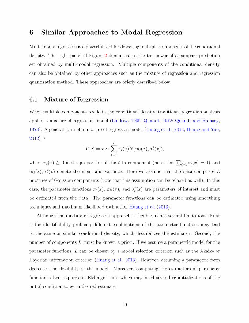
Multi-modal regression is a powerful tool for detecting multiple components of the conditional

density. The right panel of Figure 2 demonstrates the the power of a compact prediction

set obtained by multi-modal regression. Multiple components of the conditional density

can also be obtained by other approaches such as the mixture of regression and regression

quantization method. These approaches are briefly described below.

6.1 Mixture of Regression

When multiple components reside in the conditional density, traditional regression analysis

applies a mixture of regression model (Lindsay, 1995; Quandt, 1972; Quandt and Ramsey,

1978). A general form of a mixture of regression model (Huang et al., 2013; Huang and Yao,

2012) is

Y |X = x ∼L∑`=1

π`(x)N(m`(x), σ2` (x)),

where π`(x) ≥ 0 is the proportion of the `-th component (note that∑L

`=1 π`(x) = 1) and

m`(x), σ2` (x) denote the mean and variance. Here we assume that the data comprises L

mixtures of Gaussian components (note that this assumption can be relaxed as well). In this

case, the parameter functions π`(x), m`(x), and σ2` (x) are parameters of interest and must

be estimated from the data. The parameter functions can be estimated using smoothing

techniques and maximum likelihood estimation Huang et al. (2013).

Although the mixture of regression approach is flexible, it has several limitations. First

is the identifiability problem; different combinations of the parameter functions may lead

to the same or similar conditional density, which destabilizes the estimator. Second, the

number of components L, must be known a priori. If we assume a parametric model for the

parameter functions, L can be chosen by a model selection criterion such as the Akaike or

Bayesian information criterion (Huang et al., 2013). However, assuming a parametric form

decreases the flexibility of the model. Moreover, computing the estimators of parameter

functions often requires an EM-algorithm, which may need several re-initializations of the

initial condition to get a desired estimate.

20

6.2 Regression Quantization

Alternatively, the authors of Loubes and Pelletier (2017) detected multiple components in a

conditional density function by combining k-means (vector quantization; Gersho and Gray

2012; Graf and Luschgy 2007) algorithm and k-nearest neighbor (kNN) approach. Their

method is called regression quantization. To illustrate the idea, we consider a 1D Gaussian

mixture model with L distinct components. If the components are well-separated and their

proportions are similar, the a k-means algorithm with k = L will return k points (called

centers in the k-means literature) that approximate the centers of Gaussians. Thus, the

centers of k-means correspond to the centers of components in our data.

In a regression setting, the k-means algorithm is combined with kNN. To avoid conflict

in the notations, we denote the number of centers in the k-means by L, although the algo-

rithm itself is called k-means. For a given point x, we find those Xi’s within the k-nearest

neighborhood of x, process their corresponding responses by the k-means algorithm. Let

Wn,i(x) =

1k

if Xi is among the k nearest neighbor of x

0 otherwise

be the weight of each observation. Given a point x, the estimator in Loubes and Pelletier

(2017) was defined as

c1(x), · · · , cL(x) = argminc1,··· ,cL

n∑i=1

minj=1,··· ,L

Wn,i(x)‖Yi − cj‖2.

Namely, we apply the k-means algorithm to the response variable of the k-NN observations.

For correct choices of k and L, the resulting estimators properly summarize the data. Be-

cause k behaves like the smoothing parameter in the KDE, the choice of k = kn has been

theoretically analyzed (Loubes and Pelletier, 2017). However, the choice of L often relies on

prior knowledge about the data (number of components), although L can be chosen by a

gap heuristic approach (Tibshirani et al., 2001).

7 Discussion

This paper reviewed common methods for fitting modal regressions. We discussed both

uni-modal and multi-modal approaches, along with relevant topics such as large sample

21

theories, bandwidth selectors, and computational recipes. Here we outline some possible

future directions of modal regression.

• Multi-modal regression in complex processes. Although the behavior of uni-

modal regression has been analyzed in dependent and censored scenarios (Collomb

et al., 1986; Khardani et al., 2010, 2011; Ould-Saıd and Cai, 2005), the behavior of

multi-modal regression is still unclear. The behavior of multi-modal regression in

censoring cases remains an open question. Moreover, by comparing the estimator in

censored response variable cases and measurement error cases (equation (6) and (10),

respectively), we find that to account for censoring, we must change the kernel function

of the response variable, whereas to adjust the measurement errors , we need to modify

the kernel function of the covariate. Thus, we believe that the KDE can be modified

to solve the censoring and measurement error problems at the same time.

• Valid confidence band. In Chen et al. (2016a), the confidence band of the multi-

modal regression was constructed by a bootstrap approach. However, because this

confidence band does not correct bias in KDE, it requires an undersmoothing assump-

tion. Recently, Calonico et al. (2017) proposed a debiased approach that constructs a

bootstrap nonparametric confidence set without undersmoothing. The application of

this approach to modal regression is another possible future direction.

• Conditional bump hunting. A classical problem in nonparametric statistics is bump

hunting (Burman and Polonik, 2009; Good and Gaskins, 1980; Hall et al., 2004), which

detects the number of significant local modes. In modal regression analysis, the bump

hunting problem may be studied in a regression setting. More specifically, we want to

detect the number of significant local modes of the conditional density function. The

output will be an integer function of the covariate that informs how the number of

significant local modes changes over different covariate values.

22

Acknowledgement

We thank two referees and the editor for their very helpful comments. Yen-Chi Chen is

supported by NIH grant number U01 AG016976.

23

References

Attaoui, S. (2014). On the nonparametric conditional density and mode estimates in the

single functional index model with strongly mixing data. Sankhya A, 76(2):356–378.

Burman, P. and Polonik, W. (2009). Multivariate mode hunting: Data analytic tools with

measures of significance. Journal of Multivariate Analysis, 100(6):1198–1218.

Calonico, S., Cattaneo, M. D., and Farrell, M. H. (2017). On the effect of bias estimation

on coverage accuracy in nonparametric inference. Journal of the American Statistical

Association, (just-accepted).

Chacon, J. and Duong, T. (2013). Data-driven density derivative estimation, with appli-

cations to nonparametric clustering and bump hunting. Electronic Journal of Statistics,

7:499–532.

Chaouch, M., Laıb, N., and Louani, D. (2017). Rate of uniform consistency for a class of

mode regression on functional stationary ergodic data. Statistical Methods & Applications,

26(1):19–47.

Chen, Y.-C. (2017). A tutorial on kernel density estimation and recent advances. Biostatistics

& Epidemiology, 1(1):161–187.

Chen, Y.-C., Genovese, C. R., Tibshirani, R. J., and Wasserman, L. (2016a). Nonparametric

modal regression. The Annals of Statistics, 44(2):489–514.

Chen, Y.-C., Genovese, C. R., and Wasserman, L. (2016b). A comprehensive approach to

mode clustering. Electronic Journal of Statistics, 10(1):210–241.

Chen, Y.-C., Genovese, C. R., and Wasserman, L. (2017a). Density level sets: Asymptotics,

inference, and visualization. Journal of the American Statistical Association, pages 1–13.

Chen, Y.-C., Genovese, C. R., and Wasserman, L. (2017b). Statistical inference using the

morse-smale complex. Electronic Journal of Statistics, 11(1):1390–1433.

24

Cheng, Y. (1995). Mean shift, mode seeking, and clustering. Pattern Analysis and Machine

Intelligence, IEEE Transactions on, 17(8):790–799.

Collomb, G., Hardle, W., and Hassani, S. (1986). A note on prediction via estimation of the

conditional mode function. Journal of Statistical Planning and Inference, 15:227–236.

Comaniciu, D. and Meer, P. (2002). Mean shift: A robust approach toward feature space

analysis. Pattern Analysis and Machine Intelligence, IEEE Transactions on, 24(5):603–

619.

Cook, J. R. and Stefanski, L. A. (1994). Simulation-extrapolation estimation in parametric

measurement error models. Journal of the American Statistical association, 89(428):1314–

1328.

Dabo-Niang, S. and Laksaci, A. (2010). Note on conditional mode estimation for functional

dependent data. Statistica, 70(1):83–94.

Dempster, A., Laird, N., and Rubin, D. (1977). Maximum likelihood from incomplete data

via the sems algorithm. Journal of the Royal Statistical Society. Series B (Methodological),

39(1):1–38.

Efron, B. (1979). Bootstrap methods: Another look at the jackknife. Annals of Statistics,

7(1):1–26.

Einbeck, J. and Tutz, G. (2006). Modelling beyond regression functions: an application of

multimodal regression to speed–flow data. Journal of the Royal Statistical Society: Series

C (Applied Statistics), 55(4):461–475.

Fan, J., Yao, Q., and Tong, H. (1996). Estimation of conditional densities and sensitivity

measures in nonlinear dynamical systems. Biometrika, 83(1):189–206.

Fan, J. and Yim, T. H. (2004). A crossvalidation method for estimating conditional densities.

Biometrika, 91(4):819–834.

25

Fukunaga, K. and Hostetler, L. (1975). The estimation of the gradient of a density function,

with applications in pattern recognition. Information Theory, IEEE Transactions on,

21(1):32–40.

Genovese, C. R., Perone-Pacifico, M., Verdinelli, I., and Wasserman, L. (2014). Nonpara-

metric ridge estimation. The Annals of Statistics, 42(4):1511–1545.

Gersho, A. and Gray, R. M. (2012). Vector quantization and signal compression, volume

159. Springer Science & Business Media, Berlin/Heidelberg, Germany.

Good, I. and Gaskins, R. (1980). Density estimation and bump-hunting by the penalized

likelihood method exemplified by scattering and meteorite data. Journal of the American

Statistical Association, 75(369):42–56.

Graf, S. and Luschgy, H. (2007). Foundations of quantization for probability distributions.

Springer, New York, NY.

Hall, P., Minnotte, M. C., and Zhang, C. (2004). Bump hunting with non-gaussian kernels.

The Annals of Statistics, 32(5):2124–2141.

Ho, C.-s., Damien, P., and Walker, S. (2017). Bayesian mode regression using mixtures of

triangular densities. Journal of Econometrics, 197(2):273–283.

Huang, M., Li, R., and Wang, S. (2013). Nonparametric mixture of regression models.

Journal of the American Statistical Association, 108(503):929–941.

Huang, M. and Yao, W. (2012). Mixture of regression models with varying mixing pro-

portions: A semiparametric approach. Journal of the American Statistical Association,

107(498):711–724.

Hyndman, R. J., Bashtannyk, D. M., and Grunwald, G. K. (1996). Estimating and visualizing

conditional densities. Journal of Computational and Graphical Statistics, 5(4):315–336.

Kaplan, E. L. and Meier, P. (1958). Nonparametric estimation from incomplete observations.

Journal of the American statistical association, 53(282):457–481.

26

Kemp, G. C. and Silva, J. S. (2012). Regression towards the mode. Journal of Econometrics,

170(1):92–101.

Khardani, S., Lemdani, M., and Saıd, E. O. (2010). Some asymptotic properties for a smooth

kernel estimator of the conditional mode under random censorship. Journal of the Korean

Statistical Society, 39(4):455–469.

Khardani, S., Lemdani, M., and Saıd, E. O. (2011). Uniform rate of strong consistency for

a smooth kernel estimator of the conditional mode for censored time series. Journal of

Statistical Planning and Inference, 141(11):3426–3436.

Khardani, S. and Yao, A. F. (2017). Non linear parametric mode regression. Communications

in Statistics-Theory and Methods, 46(6):3006–3024.

Krief, J. M. (2017). Semi-linear mode regression. The Econometrics Journal, 20(2):149–167.

Lee, M.-j. (1989). Mode regression. Journal of Econometrics, 42(3):337–349.

Lee, M.-J. (1993). Quadratic mode regression. Journal of Econometrics, 57(1-3):1–19.

Lee, M.-J. and Kim, H. (1998). Semiparametric econometric estimators for a truncated

regression model: A review with an extension. Statistica Neerlandica, 52(2):200–225.

Li, J., Ray, S., and Lindsay, B. G. (2007). A nonparametric statistical approach to clustering

via mode identification. Journal of Machine Learning Research, 8(8):1687–1723.

Lindsay, B. G. (1995). Mixture models: theory, geometry and applications. In NSF-CBMS

regional conference series in probability and statistics, pages i–163. JSTOR.

Loubes, J.-M. and Pelletier, B. (2017). Prediction by quantization of a conditional distribu-

tion. Electronic Journal of Statistics, 11(1):2679–2706.

Manski, C. (1991). Regression. Journal of Economic Literature, 29(1):34–50.

Nadaraya, E. A. (1964). On estimating regression. Theory of Probability & Its Applications,

9(1):141–142.

27

Ould-Saıd, E. (1993). Estimation non parametrique du mode conditionnel. application a la

prevision. Comptes rendus de l’Academie des sciences. Serie 1, Mathematique, 316(9):943–

947.

Ould-Saıd, E. (1997). A note on ergodic processes prediction via estimation of the conditional

mode function. Scandinavian journal of statistics, 24(2):231–239.

Ould-Saıd, E. and Cai, Z. (2005). Strong uniform consistency of nonparametric estimation

of the censored conditional mode function. Nonparametric Statistics, 17(7):797–806.

Quandt, R. E. (1972). A new approach to estimating switching regressions. Journal of the

American statistical association, 67(338):306–310.

Quandt, R. E. and Ramsey, J. B. (1978). Estimating mixtures of normal distributions and

switching regressions. Journal of the American statistical Association, 73(364):730–738.

Rinaldo, A. and Wasserman, L. (2010). Generalized density clustering. The Annals of

Statistics, 38(5):2678–2722.

Sager, T. W. and Thisted, R. A. (1982). Maximum likelihood estimation of isotonic modal

regression. The Annals of Statistics, 10(3):690–707.

Sasaki, H., Ono, Y., and Sugiyama, M. (2016). Modal regression via direct log-density

derivative estimation. In International Conference on Neural Information Processing,

pages 108–116. Springer.

Scott, D. W. (1992). Multivariate density estimation: theory, practice, and visualization.

John Wiley & Sons, Hoboken, NJ.

Scott, D. W. (2015). Multivariate density estimation: theory, practice, and visualization.

John Wiley & Sons, Hoboken, NJ.

Sheather, S. J. (2004). Density estimation. Statistical Science, 19(4):588–597.

Silverman, B. W. (1986). Density Estimation for Statistics and Data Analysis. Chapman

and Hall, London, United Kingdom.

28

Tarter, M. E. and Lock, M. D. (1993). Model-free curve estimation, volume 56. CRC Press,

Boca Raton, FL.

Tibshirani, R., Walther, G., and Hastie, T. (2001). Estimating the number of clusters in a

data set via the gap statistic. Journal of the Royal Statistical Society: Series B (Statistical

Methodology), 63(2):411–423.

Wang, X., Chen, H., Shen, D., and Huang, H. (2017). Cognitive impairment prediction in

alzheimer’s disease with regularized modal regression. In Advances in Neural Information

Processing Systems, pages 1447–1457.

Watson, G. S. (1964). Smooth regression analysis. Sankhya: The Indian Journal of Statistics,

Series A, pages 359–372.

Wu, C. J. (1983). On the convergence properties of the em algorithm. The Annals of

Statistics, 11(1):95–103.

Yao, W. and Li, L. (2014). A new regression model: modal linear regression. Scandinavian

Journal of Statistics, 41(3):656–671.

Yao, W., Lindsay, B. G., and Li, R. (2012). Local modal regression. Journal of nonparametric

statistics, 24(3):647–663.

Zhou, H. and Huang, X. (2016). Nonparametric modal regression in the presence of mea-

surement error. Electronic Journal of Statistics, 10(2):3579–3620.

Zhou, H. and Huang, X. (2017). Bandwidth selection for nonparametric modal regression.

To appear in Communications in Statistics - Simulation and Computation.

29