Modal Acoustic Transfer Vectors Make Acoustic Radiation Models Practical for Engines and Rotating

Machinery Colin McCulloch, Michel Tournour and Pierre Guisset

LMS International, Leuven, Belgium Abstract: The paper presents Acoustic Transfer Vectors (ATVs) and Modal Acoustic Transfer Vectors (MATVs) and their use in acoustic radiation prediction, particularly from the surfaces of engines and their components and from other rotating machinery. Acoustic Transfer Vectors are input-output relations between the normal structural velocity of the radiating surface and the sound pressure at a specific point in the field. The Modal counterpart gives a similar relation, but expressed in the modal coordinates of the radiating structure. The structural response, computed with a standard FE model such as ANSYS®, can be determined either directly in the frequency domain, or (often more-efficiently) using a modal model, and this provides the boundary conditions or ‘drivers’ for the acoustic radiation.

Rotating machinery applications frequently require multiple loadcases, related to different rotational speeds such as an engine run-up, as well as multiple frequencies in the acoustic response. Using ATVs or MATVs, together with interpolation techniques, the amount of heavy computations needed to produce a large volume of results in such multi-rpm/loadcase/multi-frequency problems is dramatically reduced. A speed-up factor of 100 is common, compared to conventional BEM in which each frequency has to be solved explicitly. Re-analysis with design modifications is made possible, within timescales that make the results valuable in the product development and optimisation.

The computations are controlled by a new model- and solver-management environment, Virtual.LabTM, which provides an integrated tool for the functional performance analysis process, many different solution sequences using internal and external solvers, and graphical tools for creating meshes for acoustic radiation from the structural FE mesh.

Introduction In the automotive and other industries where there are rotating machines such as engines, or components attached to them, which radiate noise, reducing and controlling that noise is often an important functional performance criterion of the design. There are many other conflicting design attributes (weight, power, torque, fuel consumption, durability…) and it is usually too late in the development process to optimise, or even achieve a good compromise, on such parameters, once a physical prototype is available. Therefore, using predictive methods at the design stage is very attractive. Structural FE models have become standard in this process, for static and dynamic solutions. The Boundary Element Method (BEM) is also effective for acoustic radiation prediction, but suffers from the problem that the computation times are often excessive, especially when the multiple loadcases, as well as multiple frequencies, of a rotating-machinery application are taken into account. The structural analysis, usually based on a modal model and then modal superposition solution, provides boundary conditions for the acoustic radiation, but the volume of data is often very large, because of the multiple frequencies and loadcases.

The process presented in this paper, using Acoustic Transfer Vectors (ATVs) and Modal ATVs, provides a dramatic reduction in the overall computation time for acoustic radiation prediction in such applications, without losing the accuracy inherent in a proper solution of the acoustic wave behavior around the radiating surface using BEM

ATV Methodology The acoustic BEM is well established for solving acoustic radiation prediction in unbounded domains. The standard approach solves an equation system for multiple loadcases, but this can be time-consuming since

the BE matrices are full, complex and frequency-dependent, so they require assembly and inversion at each frequency.

The Acoustic Transfer Vector (ATV) concept re-organises the solution process, so that the computational effort is minimised. The ATVs are input-output relations between the normal surface velocity and the sound pressure at specific field points. They can also be referred to as contribution vectors or acoustic sensitivities, and they depend only on the surface geometry, the fluid properties (density and sound speed) and any acoustic surface treatment (locally-reacting impedance). Importantly, they do not depend on the loading (vibration boundary conditions, defined by the structural FE analysis). Therefore, the ATVs can be computed even before the structural response is known.

A highly efficient procedure for computing the ATVs has been implemented in the LMS SYSNOISE program, which limits the computational cost to the cost of a single frequency-sweep. Further to that, when exterior radiation is considered, the ATVs are rather smoothly-varying with frequency, so it is only necessary to compute them at selected (‘master’) frequencies, and the ATVs which may be needed at intermediate frequencies in the final radiation computation can be derived with sufficient accuracy by interpolation.

Once the ATVs are known, the acoustic pressure ( )ωp at a field point is computed by a rapid vector-vector product of ATV and normal vibration shape on the surface ( ){ }ωnv , which requires very little calculation time:

( ) ( ){ } ( ){ }ωωω nT vATVp = (1)

The process for computing the structural response frequently relies on modal superposition, so that:

( ){ } [ ] ( ){ }ωωω mrspjv nn Φ= (2)

where [ is the matrix of modal vectors, projected on the local normal direction of the radiating surface,

and

]}

nΦ{ ( )ωmrsp is the modal response (vector of modal participation factors). The structural analysis in a

standard FE program can provide the participation factors of the modes, at each frequency, for each loadcase.

Considering again Equation (1), we can use the mode shape vectors (for the radiating surface only) as surface vibration shapes, thus deriving Modal Acoustic Transfer Vectors as: iMATV

( ){ } { }niTi ATVjMATV φωω= ((33

}))

where { niφ iiss tthhee ((pprroojjeecctteedd)) sshhaappee vveeccttoorr ooff tthhee iith mmooddee sshhaappee.. Then, the final acoustic result is determined by multiplying the MATVs by the modal participations:

th

( ) ( ){ } ( ){ }ωωω mrspMATVp T= ((44))

Sound power derivation Using ATVs or MATVs gives only pressure results at points in the field. However, it has been found that the rules in ISO3744 for calculating radiated sound power from measured pressure data can be used in predictive models, so that sound power can be calculated from a limited number of field points (or microphone positions) with good accuracy in most applications. The microphone positions are at optimal locations related to the characteristic dimensions of the radiating object and its position versus a reflective floor (if any). In order to investigate the surface behaviour, for example to find the relative contributions to radiated power from different parts of the surface, contribution analysis techniques (also based on the ATVs) can be used, but further discussion of these techniques is beyond the scope of this paper.

Reduced data transfer and re-use of saved data Using Modal ATVs brings an important reduction in data volumes to be transferred from the FE structural model to the acoustic BE model: the mode shapes remain constant, irrespective of multiple loadcases and frequencies that may be solved structurally and acoustically. However, this introduces a dependence on the structural model: if structural design changes occur, such as modifications to stiffness, the modes will change and the MATVs have to be recomputed. If the geometry of the exterior radiating envelope surface does not change, however, the ATVs will remain as before and the additional computations are minimal. Thus, a structural optimisation procedure can be used, and can include the acoustic results as part of its objective function, without large computational costs when iterations or re-analyses are required.

Applications Two applications to the radiation of noise from automotive engines are presented:

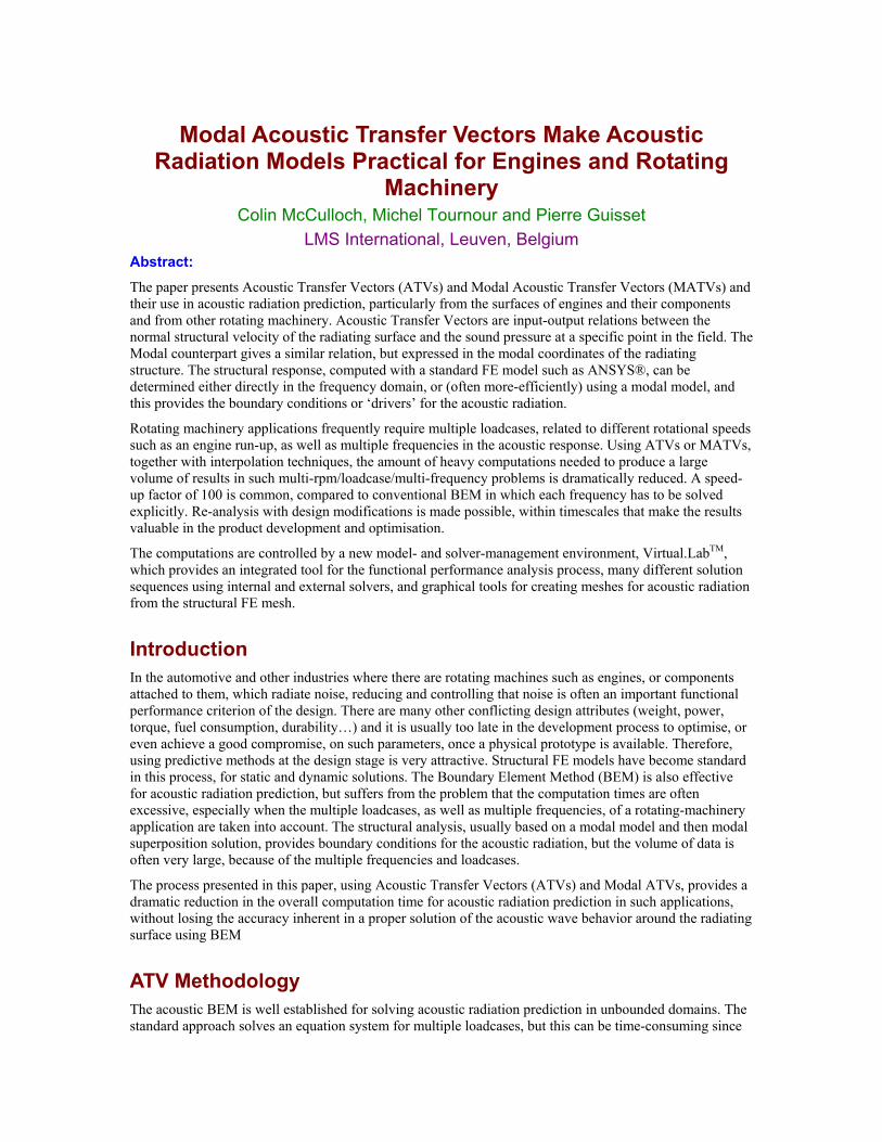
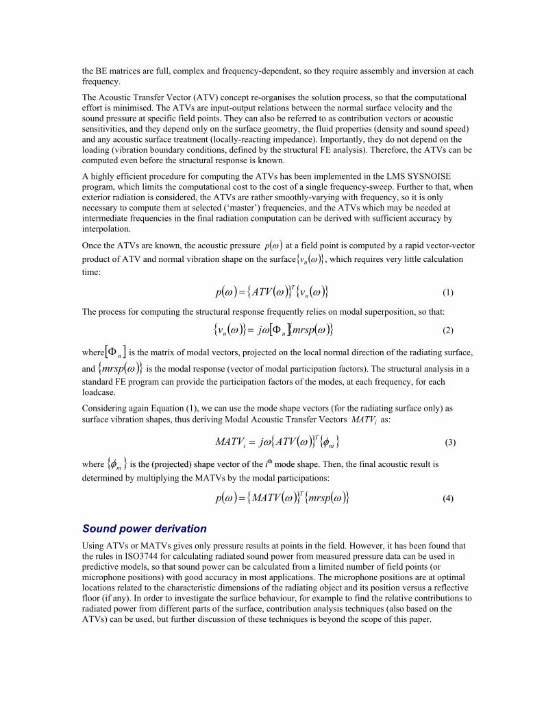
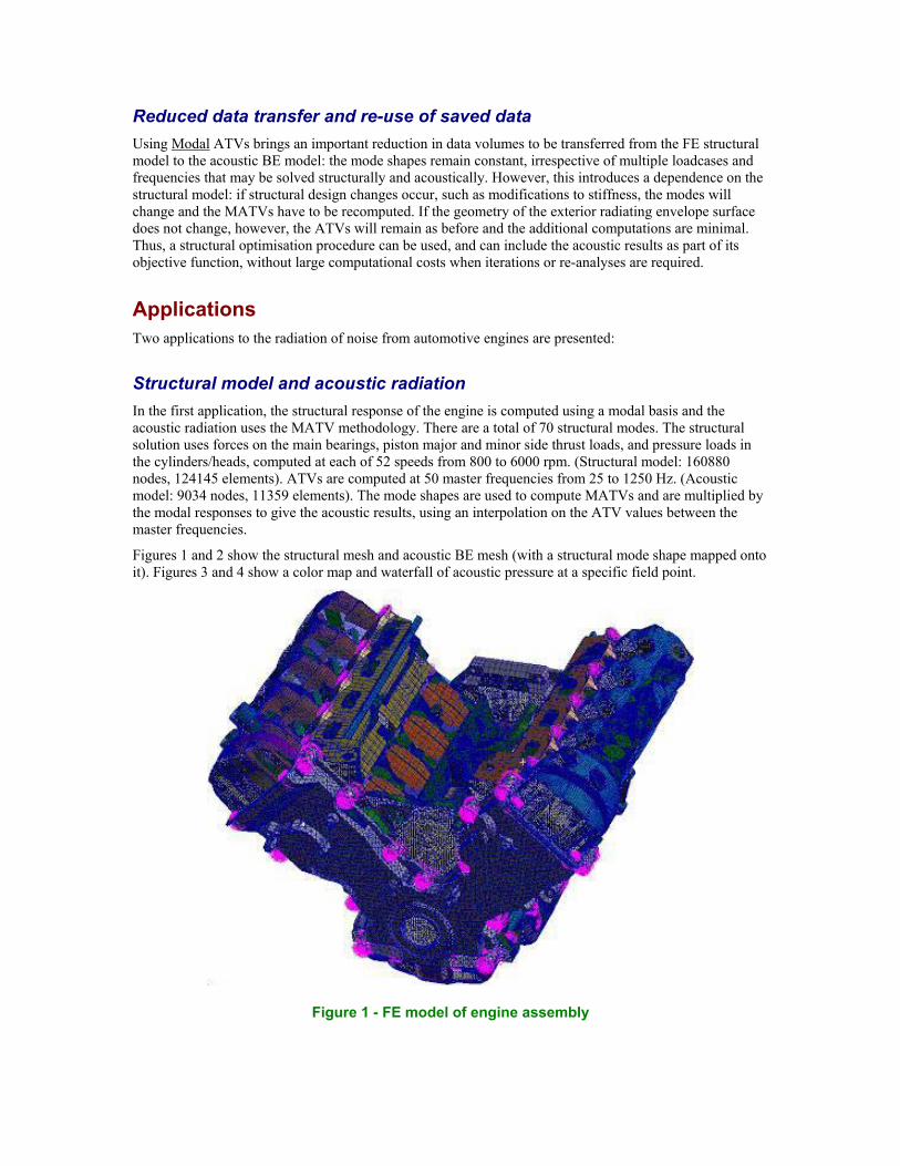
Structural model and acoustic radiation In the first application, the structural response of the engine is computed using a modal basis and the acoustic radiation uses the MATV methodology. There are a total of 70 structural modes. The structural solution uses forces on the main bearings, piston major and minor side thrust loads, and pressure loads in the cylinders/heads, computed at each of 52 speeds from 800 to 6000 rpm. (Structural model: 160880 nodes, 124145 elements). ATVs are computed at 50 master frequencies from 25 to 1250 Hz. (Acoustic model: 9034 nodes, 11359 elements). The mode shapes are used to compute MATVs and are multiplied by the modal responses to give the acoustic results, using an interpolation on the ATV values between the master frequencies.

Figures 1 and 2 show the structural mesh and acoustic BE mesh (with a structural mode shape mapped onto it). Figures 3 and 4 show a color map and waterfall of acoustic pressure at a specific field point.

Figure 1 - FE model of engine assembly

Figure 2 - Mode shape mapped on BE mesh

Figure 3 - Color map of acoustic pressure (1)

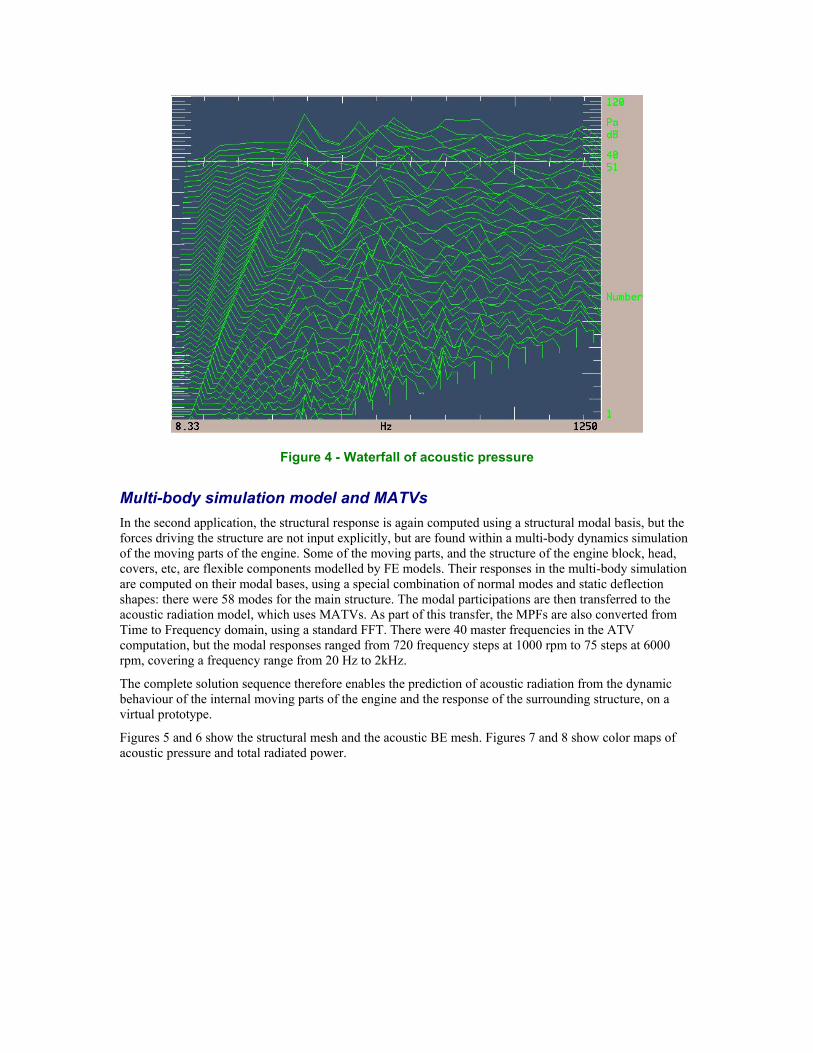
Figure 4 - Waterfall of acoustic pressure

Multi-body simulation model and MATVs In the second application, the structural response is again computed using a structural modal basis, but the forces driving the structure are not input explicitly, but are found within a multi-body dynamics simulation of the moving parts of the engine. Some of the moving parts, and the structure of the engine block, head, covers, etc, are flexible components modelled by FE models. Their responses in the multi-body simulation are computed on their modal bases, using a special combination of normal modes and static deflection shapes: there were 58 modes for the main structure. The modal participations are then transferred to the acoustic radiation model, which uses MATVs. As part of this transfer, the MPFs are also converted from Time to Frequency domain, using a standard FFT. There were 40 master frequencies in the ATV computation, but the modal responses ranged from 720 frequency steps at 1000 rpm to 75 steps at 6000 rpm, covering a frequency range from 20 Hz to 2kHz.

The complete solution sequence therefore enables the prediction of acoustic radiation from the dynamic behaviour of the internal moving parts of the engine and the response of the surrounding structure, on a virtual prototype.

Figures 5 and 6 show the structural mesh and the acoustic BE mesh. Figures 7 and 8 show color maps of acoustic pressure and total radiated power.

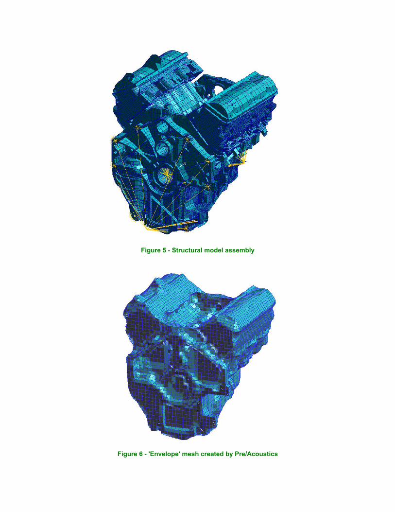
Figure 5 - Structural model assembly

Figure 6 - 'Envelope' mesh created by Pre/Acoustics

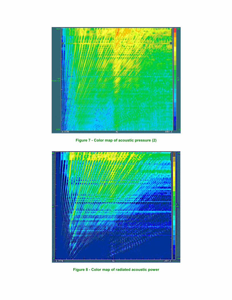
Figure 7 - Color map of acoustic pressure (2)

Figure 8 - Color map of radiated acoustic power

Remarks In both examples, it can be observed that there are both resonance-related responses (at fixed frequencies, irrespective of engine speed) and order-related responses (at frequencies varying with some multiple of engine speed). The treatment of problems (namely, high noise outputs) of these two types, is typically very different. Only by computing complete color maps or waterfalls, such as shown here, can such problems be identified and solutions investigated. As detailed below, the MATV-based solution sequence enables re-computation after making design changes, within feasible timescales.

Calculation Time Benefits The enormous speed-up in overall calculation times, from using the M/ATV method, has been reported by users in many practical cases. For the examples given above: in the first case, the ATV computation for 19 field points at 50 frequencies took about 35 hours on an HP C3000 workstation, after which the 'solve' sequence (ATVs x modes shapes x MPFs) took about 6 hours. To perform the same computation ‘directly’ using the conventional BEM approach, with a solution time of about 30 minutes per frequency and 60 frequencies at each of 52 engine speeds, would take in excess of 1500 hours.

On the second example given above (acoustic model: 7500 nodes) the ATV computation at 40 frequencies took about 10 hours on a large HP workstation (J-series) and the 'solve' sequence for a total of 21,400 frequency points, covering 1000 rpm to 6000 rpm in 50 rpm steps, took a total of 3.5 hours.

If the same solution had been attempted for 21,400 frequency steps, using a conventional BEM solution with each frequency solved separately (since frequencies are rarely identical for different RPMs) and taking 0.2 hours per frequency, the total time would have been about 180 days! The M/ATV methodology makes the impossible, practical.

A further benefit of the Modal ATV approach in particular, is that the data file sizes and file/data transfer requirements are much reduced: only structural modes have to be transferred to the acoustic model (for example from .rst files) and the modal participations at multiple frequencies and speeds are relatively very small arrays of data.

User Environment and Solution Control The ATV/MATV methodology was implemented in LMS SYSNOISE Revision 5.5 for the acoustic part of the calculations and can be used with an FE code, such as ANSYS, for the structural part. The control and execution of the process is made much easier, and integrated with other modelling and solution actions, in a new user environment, LMS Virtual.LabTM. Virtual.Lab provides a graphical user environment, with control of the solution sequence using a unique ‘specification tree’ that provides graphical insight into the process flow and inter-relationships of models and data, and a re-usable template, and visualisation of the results such as colour maps or waterfalls of multi-frequency/multi-rpm data. The Virtual.Lab structural response solution can import the structural modes from FE software such as ANSYS and compute structural (modal) responses, using loadings derived from multi-body simulations (also performed in Virtual.Lab) or imported, or acquired from measured data in a unique ‘hybrid’ approach. The modal responses can then be passed to the MATV acoustic radiation prediction, in the Virtual.Lab ATV Response solution. By linking analyses using the specification tree in an interactive and guided way, the whole process is made straightforward even for inexperienced or occasional users. Model data, results and relationships between models (for example, how an acoustic model is driven by the responses in a structural model) are all stored in single, consistent, databases.

Figure 9 shows a typical Virtual.Lab screenshot for a structural/MATV analysis.

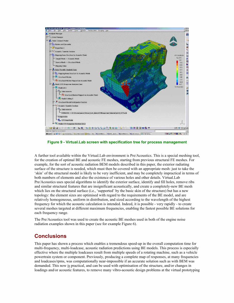
Figure 9 - Virtual.Lab screen with specification tree for process management

A further tool available within the Virtual.Lab environment is Pre/Acoustics. This is a special meshing tool, for the creation of optimal BE and acoustic FE meshes, starting from previous structural FE meshes. For example, for the sort of acoustic radiation BEM models described in this paper, the exterior radiating surface of the structure is needed, which must then be covered with an appropriate mesh: just to take the ‘skin’ of the structural model is likely to be very inefficient, and may be completely impractical in terms of both numbers of elements and also the existence of various holes and other details. Virtual.Lab Pre/Acoustics uses special algorithms to identify the exterior surface, identify and fill holes, remove ribs and similar structural features that are insignificant acoustically, and create a completely-new BE mesh which lies on the structural surface (i.e., ‘supported’ by the basic skin of the structure) but has a new topology: the element sizes are optimised with regard to the requirements of the BE model, and are relatively homogeneous, uniform in distribution, and sized according to the wavelength of the highest frequency for which the acoustic calculation is intended. Indeed, it is possible - very rapidly - to create several meshes targeted at different maximum frequencies, enabling the fastest possible BE solutions for each frequency range.

The Pre/Acoustics tool was used to create the acoustic BE meshes used in both of the engine noise radiation examples shown in this paper (see for example Figure 6).

Conclusions This paper has shown a process which enables a tremendous speed-up in the overall computation time for multi-frequency, multi-loadcase, acoustic radiation predictions using BE models. This process is especially effective where the multiple loadcases result from multiple speeds of a rotating machine, such as a vehicle powertrain system or component. Previously, producing a complete map of responses, at many frequencies and loadcases/rpms, was computationally near-impossible if an accurate solution such as with BEM was demanded. This now is practical, and can be used with optimisation of the structure, and/or changes in loadings and/or acoustic features, to remove many vibro-acoustic design problems at the virtual prototyping

stage. Building these methods into an interactive user environment for analysis process control and integration of other modeling and solution tools, further enhances control, repeatability and engineering understanding of the functional performance of the design.

Acknowledgements Figures 1 to 4 and model data and calculation times for the first example: by courtesy of Ford Motor Company, Dearborn, MI (Mr. M Felice, Mr. Abbas Selmane).

Figures 5 to 8 and model data for the second example: by courtesy of General Motors Corporation, Warren, MI.

References "Boundary Elements in Acoustics: Advances and Applications", ed. O von Estorff, WIT Press (2001).

Seybert, A F, "Review of the boundary element method in acoustics", Noise Control Foundation, New York, NY, USA 2532, 25-31 (1991).

Burton A J and Miller G F, "The application of integral equation methods to the numerical solution of some exterior boundary value problems", Proc Royal Soc, London, A323, 201-210 (1971).

"SYSNOISE Rev 5.5 Users Manual" LMS International, Leuven, Belgium (2001).