mobility and gender at the top tail of the earnings

The Economic and Social Review, Vol. 37, No. 2, Summer/Autumn, 2006, pp. 149-173

Mobility and Gender at the Top Tail of theEarnings Distribution*

ROSS FINNIEStatistics Canada

IAN IRVINEConcordia University

Abstract: The increasing share of the top fractile in the earnings distributions of several Anglo-Saxon heritage economies since the 1970s has been dramatic, and well documented. To date,however, little is known about the socio-economic origins and gender composition of the very toptail in the modern era. This paper takes a first step in filling some of the holes in our knowledge.We use a tax-filer data base for Canada for the period 1983-2003 that contains about eightymillion observations. We show first that male earners in the top one thousandth of the distributioncome very disproportionately from families with incomes in the top decile. In contrast, individualsin the remaining part of the top centile have more dispersed socio-economic origins. Second weshow that female participation in the top fractiles has been very low, and that growth inparticipation has been slow yet definite. In contrast, female earnings in this echelon are almoston par with male earnings. Third, we show that there is an enormous asymmetry between thegenders when it comes to spousal earnings: high-earning women have very high-earning spouses,but not vice versa. ‘Secondary males’ have earnings levels almost ten times as high as ‘secondaryfemales’, suggesting that, even at this extremely elevated earnings level there is truth to theadage about who lies ‘behind’ successful individuals. Finally, it is illustrated that the earningsconcentration that has characterised the last three decades did not change with the end of the‘tech boom’ in the year 2000.

149

*An earlier version was presented at the Conference on Macroeconomic Perspectives in Honour ofBrendan M. Walsh, held at University College Dublin on 7 October, 2005. Ross Finnie works atStatistics Canada, and is a Fellow of the School of Policy Studies, Queen’s University, Ontario,Canada. Ian Irvine is a Professor at Concordia University, Montreal, Quebec, Canada, H4X 1T9.The authors are grateful to Statistics Canada for providing access to the data base, to AndreBernard for excellent research assistance, and to the Journal editor and referees for comments onthe early drafts of this paper. Corresponding author is Irvine at [email protected].

I INTRODUCTION

The recent growth in share of the very top fractiles of the incomedistribution in Anglo-Saxon heritage economies has been truly

remarkable. Saez and Veall (2005) show that the pattern of gain has beenbroadly similar in the United Stated and Canada, with the latter laggingslightly: the wage-income share of the top 1 per cent has approximatelydoubled from 6 per cent to 12 per cent over the period 1975 to 2000, and theshare of the top 0.1 per cent has approximately quadrupled over the same timeframe – from just over 1 per cent to 5 per cent. These patterns are illustratedin Figures 1 and 2, which are taken from Saez and Veall.

Atkinson (2005) and Atkinson and Leigh (2004) have shown that a similarpattern characterises the data for the UK, Australia and New Zealand, thoughthe trends in the Antipodes have not been quite so strong. A recent paper forIreland – another primarily English-speaking economy – by Nolan (2005)indicates a pattern of top fractile growth similar to the economies examined byAtkinson and Leigh. Piketty and Saez (2003) initially charted the patterns for

150 THE ECONOMIC AND SOCIAL REVIEW

Figure 1: Top Decile Shares, Canada

Source: Saez and Veall (2005).

the US. In contrast, many other studies have found no such pattern in thedata for France (Piketty, 2003), Japan (Moriguchi and Saez, 2005), theNetherlands (Atkinson and Salverda, 2005), Switzerland (Dell, Piketty andSaez, 2005) or Spain (Alvaredo and Saez, 2005) as examples.

Such a growth in concentration raises a number of questions about thoseindividuals who inhabit the very top echelon of the distribution: what is thedegree of social mobility in this world? Does there exist a ‘glass ceiling’ forwomen that restricts their participation in this group? For those women whoare members of this elite, are their earnings comparable to male earnings?What are the spousal earnings of individuals in the top fractiles? How havethese patterns evolved in recent decades? To date the literature has shed verylittle light on these issues.

These questions are of interest not just to economists, but to sociologistsand public policy makers broadly defined. In the present paper we explorethese questions and succeed in providing answers with the help of aremarkable data base composed of about 80 million Canadian tax filers. Whilewe obviously cannot generalise our findings to other economies, even English-

MOBILITY AND GENDER IN EARNINGS DISTRIBUTION 151

Figure 2: Top Decile Shares, Canada and the US

Source: Saez and Veall (2005).

speaking ones, our results will hopefully motivate similar investigationselsewhere.

But first, why are we interested? For some, the concentration of incomeand/or wealth may be just the inevitable consequence of the incentivesnecessary for a more efficient functioning of a market economy. If this is so,then we could take the position that, provided the poor are not completelydestitute, there is little reason for concern: the growth in the top tail incomesmay not have been at the expense of those at the bottom in the distributionand, therefore, any resulting increase in inequality or polarisation may notreflect a worsening of the absolute status of the poor.

An alternative perspective sees polarisation as potentially welfarereducing, even if it is brought about by an increase in the distance of the toptail from the median without increasing the distance between the median andthose in the lower tail. Increased polarisation may result in elevated crimerates or even social disintegration in the extreme (Diamond, 2005).1 Crimemay also spread in less equal societies (Fajnzylber, Lederman and Loayza,2002) because the opportunity costs to the disenfranchised fall. Rioting bymarginalised groups in France in the Autumn of 2005 was arguably areflection of the divide between insiders and outsiders.2

A second consequence of increasing income spreads is reduced socialmobility. Higher incomes in the upper centiles reduce the likelihood ofintergenerational income mobility as a result of bequests and trusts. Recentevidence (Corak, 2004) suggests that social mobility in the US may now be aslow as some of ‘Old Europe’, although mobility in Canada is high, despite therecent surge in top incomes there. Reduced mobility may also result from amore easily acquired and financed education on the part of the offspring ofthose with very high incomes.

Third, increases in income concentration at the top tail cannot but lead toincreases in the concentration of wealth. Kennickell (2001), indicates that thetop 1 per cent of the US wealth distribution now owns about 35 per cent of allpersonal wealth, the next 9 per cent, owns about one-third, and the remaining90 per cent of the population owns less than one-third. Concentrations ofwealth also lead to reduced social mobility, and an increase in political power.Glaeser (2005) proposes that greater concentrations of wealth can increase thelobbying and political power of those at the upper tail and thereby increaseinequality further.


1As an example, The Washington Post reported in September 2005 that, in Brazil, 36,000 peoplehad been killed with guns in 2004. Sala-i-Martin (2002) indicates that Brazil’s income distributionnot only displays much more inequality than virtually all countries at a comparable level ofdevelopment, but that it is actually bimodal.2Duclos, Esteban and Ray (2004) examine the link between alienation and polarisation.

Fourth, greater polarisation may decrease the demand for common publicgoods. The rich may prefer gated communities built around golf courses withtheir own security forces, road maintenance, and local public goods, while thegreater part of the income distribution may desire more public-schoolinvestment. A substantial literature (e.g., Alesina, Baqir and Easterly, 1999)exists on this, that shows not only does the polarisation of demands, itselfdriven by income polarisation, decrease redistributive possibilities, but canalso lead to inefficient levels of human capital investment for the economy atlarge.

Finally there is the question of public policy. If it is desirable to place somelimit on polarisation, or income/wealth concentration, it is necessary tounderstand why and how the observed concentrations develop and change. Arethe giant shifts in shares recently observed the result of taxation policy, orchanges in social norms, or the fruits of invention, technological shocks andluck? If public policy measures have indeed been behind these seismic shifts,then we need to understand the linkages between public policy andwealth/income concentrations.

Understanding why earnings have become so concentrated at the top tailis additionally important in view of the role that has been attributed totechnological change in the last decade. The accepted wisdom is thattechnological change has been of the skill-biased type, and hence benefitedthose with high skills and incomes. At the same time, the fact that only the top1 per cent of the distribution has increased its share of total earnings inCanada (and several of the English-speaking economies) in a substantial way,whereas one would expect that the whole of the top decile at least would havebenefited from skill-biased technological change, raises the possibility that thebenefits of skill-biased technological change have been largely appropriated bya very small group. Eckstein and Nagypal (2004) indicate that the returns toeducation have been very non-linear, and that postgraduates, rather thanuniversity graduates at large, have gained disproportionately in the last threedecades in the US. Postgraduates are very small in number and therefore thispattern is consistent with what emerges from an examination of the very toptail of the earnings distribution.

Saez and Veall (2005) and Piketty and Saez (2003) have each proposedthat the growing share of the top fractiles can be understood best as reflectingprimarily a change in social norms – at least in Anglo-Saxon heritageeconomies, rather than being attributable to a change in tax structure (assuggested by Feldstein (1995)), the impact of skill-biased technological change,or the spectacular growth of stock options in the nineties.

The current paper examines the characteristics of those individuals whocompose the top echelons of the distribution. In line with recent practice, we


compare the top one thousandth of the distribution with the remainder of thetop centile and in turn with the remainder of the top decile and the rest of thepopulation. We first focus on intergenerational mobility. Buchinsky and Hunt(1999) have found that income mobility has lessened substantially in the USin recent decades. They used a representative sample from the NLSY. Incontrast we investigate the extreme top tail of the distribution – though ourdata do not permit us to examine how mobility has changed over time – forreasons that will become clear in our discussion of the data. Second, weexamine the composition of the top fractiles from a gender standpoint. Thereexists an extensive literature on women in the labour market, and a subset ofthis focuses upon what is termed the ‘glass ceiling’ – proposing that thereexists a less visible set of obstacles to the progress of women into the very topsalary ranks. As part of this search we examine the earnings of spouses ofthose in the top fractiles. In each case the novelty of the present work springsfrom the fact that we examine the extreme top of the income distribution, afocus made possible by our access to tax-based data that accurately capturesthis tail.

II DATA

The Longitudinal Administrative Database (LAD) represents a 20 per centlongitudinal sample of Canadian tax-filers constructed from Canada Customsand Revenue Agency (CCRA – previously Revenue Canada) tax files. The firstyear of data is 1983 and the LAD currently goes to 2003, thus determining theperiod covered by this analysis. The relatively recent final year of the dataallows us to examine patterns in the post tech-bubble period. The LAD filepossesses on the order of five million observations per recent year, and thework reported here is based on the full LAD base, making for generoussamples at the extremes of the distribution.

Individuals are selected into the LAD according to a random numbergenerator based on Social Insurance Numbers (SINs) and are followed overthe time by the same means.3 Individuals drop out of the LAD if they do notfile taxes, or if they die or emigrate, while new filers are continually added tothe database in the fixed 20 per cent of population ratio. The size of the filehas grown over time, commensurate with the growth in the underlying tax-filing population.


3Individuals are tracked across any changes in their SIN, an event that characterisesapproximately 3 per cent of all tax filers in any given year.

The LAD’s coverage of the adult population is good since the rate of taxfiling is very high. Higher- and middle-income Canadians are required by lawto do so, while lower income individuals have incentives to file in order torecover income tax and other payroll tax deductions made through the yearand, since 1986, to benefit from various tax credits and the National Child TaxBenefit introduced in the nineties. The full set of tax files from which the LADis constructed are estimated to cover upwards of 90 per cent of the targetpopulation, thus comparing favourably with other databases. Furthermore, ahigh proportion of those not included are non-labour market participants(older married women in particular), and it is on account of this status thatthey do not file taxes.4 But from the standpoint of the present study, the LADhas a very comprehensive coverage of those at the top end of the incomedistribution. Moreover, the work of Saez and Veall is partly based on this dataset, and therefore our estimates are comparable to theirs.

The LAD includes information derived from individuals’ tax files: basicdemographic characteristics, income (sources, amounts), deductions, and taxpaid.5 Important to this analysis is the quality of the income information: theincome variable is constructed in a consistent manner over the full period weanalyse.6

When sorting individuals into family units, the main criterion is theaddress of the individual(s). This means that both common law and standard(legal) marriages are recognised. The resulting household unit thereforecorresponds closely to what is usually termed an ‘economic’ family – one thatshares resources by virtue of living at the same domicile. The data are alsocharacterised by a constant definition of the filing unit, unlike many othereconomies’ data bases, where the filing unit has changed from the family to theindividual, or gives the option of filing in either status (see, for example, thediscussion in Atkinson and Leigh (2004)).

III SAMPLE SELECTION

Most of the samples in our analysis are constructed by imposing thefollowing restrictions on a year-by-year (cross-sectional) basis. First, individ-uals had to be between 20 and 59 years of age in a given year, thus eliminating


4See Atkinson et al. (1992) for discussion of the general advantages of administrative data of thistype over survey data in terms of sample representation, the accuracy of the information collected,and in other ways.5For those matched into families, information pertaining to the other family members and therelevant family totals are appended to individuals’ records.6For most of its surveys, Statistics Canada now attempts to gain participants’ permission to usetheir tax files to gather data on incomes.

many students and semi-retired workers whose earnings tend to be low and tovary from year-to-year for their own special reasons. Second, full-time post-secondary students were excluded (based on various tuition and othereducation-related deductions) on the grounds that they have a diminishedattachment to the labour force and their earnings do not necessarily reflectlabour-market opportunities. The results of applying these selection criteria tothe 20 per cent of population LAD yielded samples for the top one thousandthof the distribution of between two and three thousand individuals in each year.

3.1 Social MobilityEconomic and social immobility between generations is a particular

consequence of economic inequality. Societies may be more willing to tolerateinequalities and extremes if such mobility is high rather than low. NorthAmerican economies were traditionally thought of as being more open andmobile than the ‘old world’ economies of nineteenth-century Western Europe.But that appears to have changed in the twentieth century. Scandinavianeconomies not only have lower rates of poverty and inequality than the US andCanada but have higher rates of intergenerational economic mobility than theUS. In addition, the Canadian and US economies have diverged whereintergenerational mobility is concerned.

Figure 3 below is from Corak (2004). It plots various intergenerationalelasticity values relating mostly the earnings of fathers and sons. Among thethree English-speaking economies, the similarity of top tail share growthbreaks down when it comes to intergenerational mobility. Elasticites for theUS and UK are substantially higher than for Canada, whose estimates lie inthe ‘Scandinavian range’. The technical details of this literature were firstmapped out by Solon (1989) and (1992). Corak emphasises that method-ological differences explain much of the variability in the US results and,therefore, care must be exercised in cross-country comparisons.

While the Forbes Four Hundred yields socio-economic information on asmall number of very top wealth holders, to our knowledge no work has yetbeen undertaken that explicitly focuses upon the socio-economic origins ofthose in the very top tail of the distribution. Since the LAD begins in the earlyeighties it affords the potential to explore the backgrounds of relatively youngindividuals currently in the top tail: tracing the parental income stratum ofcurrent high earners involves locating these earners in their parental familywhile they were still members of that household, which is when they were intheir late teens. Accordingly, our strategy is to take all individuals in the LAD falling in the age bracket 35-38 years in the year 2003, and seek to locate their parental ‘family market income’ decile approximately twenty yearsearlier. We then compute transition probabilities for the top tail of this


distribution of young earners – the top decile, the top 1 per cent and the top0.1 per cent.

Our strategy obviously does not uncover the family background of all theyoung high-earning individuals. For example, they may come from immigrantfamilies who were not domiciled in Canada in the early eighties, or theirparents may not have filed a tax return in the early eighties. Table 1 containsthe first set of results. Each number in that table is rounded to a 0 or 5.Consequently, the zero elements that appear in the top fractile column can beinterpreted as ‘small number’ rather than as a strict zero. It is evident thatlow-value cells, such as those containing ‘0’ or ‘5’, limit the conclusions that canbe drawn.

We identified 370,205 individuals in the 2003 LAD sample in the agegroup 35-38 years, and then attempted to locate each of these individuals in atleast one of the years 1982, 1983, 1984. Approximately half were not located(182,865), and some of those located were living as independents rather thanin a family context (56,685). This means that the family background wasidentified for about 35 per cent of the 2003 distribution of young earners. Foreach year 1982, 1983, 1984 all families in the LAD were ranked by incomedecile. When the family in which a 2003 earner resided was identified, thedecile rank of the family was associated with the young earner. The parental


Note: Each vertical bar represents the value of a reported earnings elasticity. Source: Corak (2004).

Figure 3: Intergenerational Earnings Elasticities

Within and cross-country variations in reported generational earnings elasticities forfathers and sons.

US

UK

FRANCE

GERMANY

SWEDEN

NORWAY

CANADA

FINLAND

DENMARK

Inherited Earnings Advantage

decile search was started in 1984 and continued back to the earlier years if theindividual was not located in the later of the three base years.

There are two well-known challenges in getting reliable estimates ofintergenerational income correlations. The first was initially addressed bySolon (1992), who showed that the intergenerational earnings correlationcoefficient is biased downward if the annual observed income of the parentdiffers from the parent’s permanent income. The results in Table 1 are basedon a single year’s parental income. Using multiple years for the parentalincome is feasible, though it would result in a loss of sample size. Nonetheless,there are two reasons why the bias in our results is likely minimal. First, weuse family income rather than individual parental income or individualparental earnings. The use of a family measure reduces the year-to-yearvariation compared to an individual-based measure. In addition, income is abroader measure of household well-being than earnings alone.

The second challenge concerns the point in the lifecycle at which theparents are observed. Grawe (2006) shows that this is a key element inreconciling the differing estimates of intergenerational mobility found in USdata. To address the possibility that age rather than socio-economicbackground may be driving the results, we estimated the average decile age ofthe parents of each of the four quantiles in Table 1 (this was not possible formuch of the very top quantile on account of the small numbers involved). Two


Table 1: Unadjusted Transition Matrix: Parental Income – Offspring Earnings

Offspring Earnings QuantileParental Family Market income 1–90 (low) 91–99 99.1–99.9 99.91–100 Total

Decile 1 (low) 3,700 205 15 0 3,920Decile 2 6,200 435 30 0 6,665Decile 3 7,395 670 35 5 8,105Decile 4 8,435 830 65 0 9,330Decile 5 9,655 1,020 65 10 10,750Decile 6 10,760 1,265 95 5 12,125Decile 7 12,595 1,665 135 10 14,405Decile 8 15,385 2,300 180 15 17,870Decile 9 18,320 3,405 325 25 22,075Decile 10 (high) 19,440 5,000 815 130 25,385Total located in 80s 111,885 16,795 1,760 200 130,630Not observed in 80s 182,865Observed in 80s not with parents 56,685Total 2003 370,205

patterns emerge from this search. First, lower-decile parents tend to beyounger than higher-decile parents, as a basic life-cycle model would predict.Despite this, there is very minimal variation in the age of parents within agiven decile across earnings quantiles of their children: parents in a givendecile whose offspring are high earners are no different age-wise than parentswhose offspring are low earners.

The next data challenge relates to the decile size of the located households:Table 1 indicates that many more individuals who were 35-38 years in 2003 were located in the upper deciles of the eighties distribution than in the lower deciles. This is illustrated in the final column. For example, theninth decile of parents contains 17 per cent of located young earners(22,075/130,630), while the second-from-bottom decile contains just 5 per cent(6,665/130,630).

The lower representation from lower-decile parents means that theoffspring of such parents were less likely to be filing a tax return while stilldomiciled in the parental home. Whether this means they were less likely towork, or less likely to have an income sufficient to warrant filing, or whetherthey have disproportionately left home (and hence among the 56,685individuals we have located in this category) cannot be established. Teenagersin Canada tend to apply for a social insurance number when they begin towork. Despite this pattern, we show below that this differential retrieval rateshould not affect the main conclusions.

The transitions data in Table 1, unadjusted for differential retrieval rates,indicate that the top 0.1 per cent of earners comes disproportionately from topdecile families. Of the 200 whose origins were traced, 130 come from the topdecile. Even allowing for the different retrieval rates for the parental deciles,there is a substantial difference in the probability of a top earner coming fromthe top parental decile as opposed to the ninth parental decile. The adjustedprobability is approximately four and a half times higher: if the 25 individualswhose parents are in the ninth decile are weighted by the relative recoveryratio (25,385/22,075) the 25 becomes 29 and therefore the relative probabilityof a top one thousand earner coming from the top parental decile is 4.5 timesthe probability of coming from the next decile (130/29 = 4.5). Yet the prob-ability of coming from the ninth parental decile is not very different from theprobability of coming from any of the fifth to eighth deciles. Sample sizes hereare small and caution is obviously appropriate.

The transition probabilities based on rescaled values are presented inTable 2. For illustration: the retrieval rate for decile 10 was 1.72 times theretrieval rate for decile 7 (25,385/14,405 = 1.72). Scaling all numbers in Table1 by their own retrieval rates and calculating the transition probabilitiesbased on these scaled values yields the probabilities in Table 2.


Our first conclusion is, therefore, that even accounting for differentretrieval rates, an earner in the top 0.1 per cent of the distribution has agreater than 50 per cent probability of coming from the top decile of theparental income distribution, but we cannot discern meaningful differences inthe probability of coming from immediately lower deciles.

In contrast, for the remainder of the top 1 per cent of the young earnersdistribution, the relative probability of coming from the top parental decile ismuch smaller – about twice as high as coming from the ninth decile and threetimes as high as the probability of coming from the eighth decile. Proceedingdown the parental distribution, the probabilities of coming from these lowerdeciles decline more smoothly than in the case of the top 0.1 per cent.Considering finally the origins of those in the remaining nine centiles withinthe top decile, the pattern is much more akin to what is observed for the 99.1– 99.9 fractile than for the 99.91 – 100 fractile: a relatively smooth anddeclining probability function.

In sum, the pattern defining the socio-economic origins of the extreme topof the earnings distribution is different from the patterns defining theremaining parts of the top decile of young earners. For those in the top onethousandth of the distribution, the probability of coming from the top decile ofthe parental distribution is in excess of 50 per cent, and the probabilities ofcoming from other deciles do not decay smoothly as they do with the otherparts of this top earnings decile.

The sample size was not sufficiently large to permit a breakdown of thesetransition probabilities between men and women. Only about 10 per cent ofthe top 0.1 per cent are women. From a total of 200 individuals retrieved for


Table 2: Transition Probabilities Adjusted for Retrieval Differentials

Offspring Earnings QuantileParental Family Market Income 1–90 (low) 91–99 99.1–99.9 99.91–100

Decile 1 (low) 0.11 0.05 0.04 0.00Decile 2 0.11 0.06 0.05 0.00Decile 3 0.10 0.08 0.04 0.06Decile 4 0.10 0.08 0.07 0.00Decile 5 0.10 0.09 0.06 0.10Decile 6 0.10 0.10 0.08 0.04Decile 7 0.10 0.11 0.09 0.07Decile 8 0.10 0.12 0.10 0.09Decile 9 0.09 0.14 0.15 0.12Decile 10 (high) 0.09 0.18 0.32 0.53

this fractile the percentage formed by women is much too small given thatindividuals must be allocated across all parental deciles.

Finally, there is the possibility that the difference in retrieval rates acrossparental deciles may bias the results. In Table 2 the retrieved data were scaledassuming that the ‘missing’ individuals come from the parental distribution inthe same proportion as the observed individuals. However, it is more likelythat the ‘undiscovered’ individuals come disproportionately from the lowerparts of the parental decile. Those individuals not included in the 130,630belong to three main groups: children of parents who migrated to Canada after1984; children observed to be living outside of the parental household(numbering 56,685) and a large remaining number, most of whom would havebeen living in the parental household without a social insurance number.

It is difficult to say anything definite about the likely placement of thoseof immigrant origin. However, for the second group – those individuals livingindependently in their late teens, it is less likely that they went to universityor obtained third level education than those who continued to live in theparental household, and therefore it is less probable that they would show upin the top part of the earnings distribution of 35-38 year olds in 2003. Thelargest missing group is likely those with no social insurance number and stillliving at home in the early eighties. Since most teens in Canada obtain a SINwhen they first take a temporary job, our ‘retrieved’ individuals are likelythose who have some employment income while a teen and living at home,while the ‘unretrieved’ individuals have not a SIN and hence unlikely to haveincome as a teen. For our results to be overstated we would have to believethat teens who have no income are more likely to be successful later in lifethan teens who do have some income. Such an argument is difficult to support.

3.2 Top Fractile Representation of WomenA body of literature now exists that focuses upon wage disparities between

men and women at different parts of the distribution. A ‘glass ceiling’ is theterm that is frequently used to describe a situation when the conditionaldistribution of earnings for one group – in this case women – differs from thatof another – men. Albrecht et al. (2003) is an example. They find this kind ofdisparity characterises the distributions in Sweden.

While our prime interest is in the extreme top of the distribution, findingsfor four components of the distribution are presented in Table 3: the top 0.1per cent, the next 0.9 per cent, the following 9 per cent and then the ‘bottom’90 per cent. This enables us to compare the representation of women with menat different points at the top of the distribution. Table 3 contains theproportion of the quantiles composed of women for a series of years between1983 and 2003. We have computed the statistics for every year, but since the



Tabl

e 3:

Ear

nin

gs D

istr

ibu

tion

s C

har

acte

rist

ics

by G

end

er

Qu

anti

leC

oun

tQ

uan

tile

Fem

ale/

Mea

nF

emal

e/S

um

Mal

eE

arn

ings

Mal

eC

atch

-up

Ind

ex (

alph

a)N

um

bers

Ear

nin

gs0.

20.

50.

8

1983

0–90

F1,

225,

100

7,90

00–

90M

98,3

840

2208

940

1.25

14,6

000.

5490

.1–9

9F

26,3

3038

,400

90.1

–99

M19

4,58

522

0915

0.14

40,3

000.

950.

800.

640.

3699

.1–9

9.9

F1,

195

77,2

0099

.1–9

9.9

M20

,900

2209

50.

0678

,400

0.98

0.90

0.76

0.44

99.9

1–10

0F

110

219,

900

99.9

1–10

0M

2,35

024

600.

0523

0,80

00.

950.

910.

790.

48

1985

0–90

F1,

232,

935

9,20

00–

90M

999,

825

2232

760

1.23

16,4

000.

5690

.1–9

9F

27,1

1042

,800

90.1

–99

M19

6,17

522

3285

0.14

44,7

000.

960.

800.

640.

3599

.1–9

9.9

F1,

500

87,7

0099

.1–9

9.9

M20

,830

2233

00.

0788

,600

0.99

0.88

0.73

0.41

99.9

1–10

0F

115

279,

900

99.9

1–10

0M

2,37

024

850.

0527

5,30

01.

020.

910.

780.

45

1987

0–90

F1,

289,

205

10,4

000–

90M

1,04

4,60

023

3380

51.

2318

,000

0.58

90.1

–99

F32

,130

47,3

0090

.1–9

9M

201,

260

2333

900.

1649

,300

0.96

0.77

0.61

0.33

99.1

–99.

9F

2,01

599

,300

99.1

–99.

9M

21,3

2523

340

0.09

101,

500

0.98

0.85

0.70

0.39

99.9

1–10

0F

160

257,

900

99.9

1–10

0M

2,43

525

950.

0733

8,50

00.

760.

890.

780.

53

MOBILITY AND GENDER IN EARNINGS DISTRIBUTION 163Ta

ble

3: E

arn

ings

Dis

trib

uti

ons

Ch

arac

teri

stic

s by

Gen

der

(co

ntd

)

Qu

anti

leC

oun

tQ

uan

tile

Fem

ale/

Mea

nF

emal

e/S

um

Mal

eE

arn

ings

Mal

eC

atch

-up

Ind

ex (

alph

a)N

um

bers

Ear

nin

gs0.

20.

50.

8

1989

0–90

F1,

354,

570

12,3

000–

90M

1,13

4,26

524

8883

51.

1920

,600

0.60

90.1

–99

F35

,285

55,1

0090

.1–9

9M

213,

600

2488

850.

1757

,300

0.96

0.77

0.60

0.32

99.1

–99.

9F

2,27

012

8,60

099

.1–9

9.9

M22

,620

2489

00.

1013

3,60

00.

960.

840.

690.

3999

.91–

100

F18

550

9,90

099

.91–

100

M2,

580

2765

0.07

574,

900

0.89

0.88

0.75

0.46

1991

0–90

F1,

394,

390

13,1

000–

90M

1,18

2,74

025

7713

01.

1819

,900

0.66

90.1

–99

F46

,485

59,0

0090

.1–9

9M

211,

230

2577

150.

2261

,800

0.95

0.70

0.54

0.29

99.1

–99.

9F

2,54

513

0,60

099

.1–9

9.9

M23

,230

2577

50.

1113

6,70

00.

960.

830.

680.

3899

.91–

100

F17

041

3100

99.9

1–10

0M

2,69

528

650.

0649

1,90

00.

840.

890.

770.

50

1993

0–90

F1,

458,

190

13,2

000–

90M

1,23

2,11

526

9030

51.

1819

,500

0.68

90.1

–99

F55

,645

61,5

0090

.1–9

9M

213,

385

2690

300.

2664

,200

0.96

0.66

0.50

0.26

99.1

–99.

9F

2,94

513

7,40

099

.1–9

9.9

M23

,955

2690

00.

1214

3,80

00.

960.

810.

660.

3799

.91–

100

F19

547

5,10

099

.91–

100

M2,

795

2990

0.07

560,

400

0.85

0.89

0.76

0.49


Tabl

e 3:

Ear

nin

gs D

istr

ibu

tion

s C

har

acte

rist

ics

by G

end

er (

con

td.)

Qu

anti

leC

oun

tQ

uan

tile

Fem

ale/

Mea

nF

emal

e/S

um

Mal

eE

arn

ings

Mal

eC

atch

-up

Ind

ex (

alph

a)N

um

bers

Ear

nin

gs0.

20.

50.

8

1995

0–90

F1,

484,

595

13,8

000–

90M

1,25

9,70

027

4429

51.

1820

,300

0.68

90.1

–99

F55

,475

64,1

0090

.1–9

9M

218,

970

2744

450.

2567

,300

0.95

0.67

0.51

0.27

99.1

–99.

9F

3,34

015

0,20

099

.1–9

9.9

M24

,110

2745

00.

1415

8,50

00.

950.

800.

640.

3599

.91–

100

F21

553

9,10

099

.91–

100

M28

3530

500.

0860

6,80

00.

890.

880.

740.

46

1997

0–90

F1,

495,

185

14,8

000–

90M

1,27

2,80

027

6798

51.

1721

,600

0.69

90.1

–99

F56

,380

68,5

0090

.1–9

9M

220,

425

2768

050.

2671

,800

0.95

0.67

0.51

0.27

99.1

–99.

9F

3,68

517

7,30

099

.1–9

9.9

M23

,995

2768

00.

1518

5,90

00.

950.

780.

620.

3499

.91–

100

F22

068

6,60

099

.91–

100

M2,

855

3075

0.08

827,

500

0.83

0.88

0.75

0.48

1999

0–90

F1,

513,

720

16,4

000–

90M

1,28

4,41

527

9813

51.

1823

,500

0.70

90.1

–99

F60

,325

74,6

0090

.1–9

9M

219,

495

2798

200.

2777

,800

0.96

0.65

0.49

0.25

99.1

–99.

9F

3,97

519

9,60

099

.1–9

9.9

M24

,005

2798

00.

1721

0,30

00.

950.

770.

600.

3399

.91–

100

F27

582

5,00

099

.91–

100

M2,

835

3110

0.10

989,

200

0.83

0.85

0.72

0.46

MOBILITY AND GENDER IN EARNINGS DISTRIBUTION 165Ta

ble

3: E

arn

ings

Dis

trib

uti

ons

Ch

arac

teri

stic

s by

Gen

der

(co

ntd

.)

Qu

anti

leC

oun

tQ

uan

tile

Fem

ale/

Mea

nF

emal

e/S

um

Mal

eE

arn

ings

Mal

eC

atch

-up

Ind

ex (

alph

a)N

um

bers

Ear

nin

gs0.

20.

50.

8

2001

0–90

F1,

536,

650

18,5

000–

90M

1,32

2,72

528

5937

51.

1625

,900

0.71

90.1

–99

F65

,670

82,3

0090

.1–9

9M

220,

270

2859

400.

3086

,000

0.96

0.62

0.47

0.24

99.1

–99.

9F

4,44

523

1,90

099

.1–9

9.9

M24

,150

2859

50.

1824

3,30

00.

950.

740.

580.

3199

.91–

100

F28

51,

058,

600

99.9

1–10

0M

2,89

531

800.

101,

237,

100

0.86

0.85

0.71

0.44

2003

0–90

F1,

549,

380

19,6

000–

90M

1,33

5,56

028

8494

01.

1627

,000

0.73

90.1

–99

F72

,110

86,7

0090

.1–9

9M

216,

410

2885

200.

3390

,800

0.95

0.59

0.44

0.23

99.1

–99.

9F

4,75

023

7,10

099

.1–9

9.9

M24

,100

2885

00.

2024

9,20

00.

950.

730.

570.

3199

.91–

100

F32

01,

012,

900

99.9

1–10

0M

2,88

532

050.

111,

173,

500

0.86

0.83

0.69

0.43

numbers are not highly cyclical, just a subset of the years is presented. Thesmallest sample in any year in this table is of the order of two and a halfmillion individuals.

The ‘female/male numbers’ column contains the percentage of eachspecified quantile that is composed of females. This ratio attains a value of0.11 for the top 0.1 per cent of the distribution in the most recent year of dataavailability – 2003 – starting from 0.05 in 1983. Its ascent has been gradual,with a stumble that coincided with the early nineties recession. The growth ofthis statistic in the remaining part of this top centile has been more rapid: ithas increased from just over 0.06 to 0.20. Furthermore, the share appears notto have been impacted by the nineties recession. The ratio in the remainder ofthe top decile (excluding the top 1 per cent) has increased from 0.14 to 0.33.(Of course, the share of females in these deciles is smaller than the foregoingfractions, being the ratio of the number of females to the total, rather than tothe number of males).

Evidently these percentages are small, and rates of share growth are low.At the same time it is not the case that progress is only outside of the topcentile. There may be a glass ceiling, but it is receding slowly throughout thewhole upper decile.

These participation rates tell us nothing about the distribution of maleand female earnings within the various quantiles. In particular, the very topof the distribution is likely characterised by a heavily skewed, perhaps Pareto,tail and it may be optimistic to believe that women and men are distributed inthe same manner throughout this tail. We have, therefore, computed theaverage income level of men and women in each of the quantiles. These aregiven in the next column headed ‘mean earnings’ and the following column‘female/male earnings’ defines the relative mean earnings values.Interestingly, the shortfall of female earnings is small and there is no strongpattern over time for this top 0.1 per cent of earners. The same pattern holdstrue for the remainder of the top centile and the remainder of the top decile.

Since the averages for women are generally below the averages for men,the lower participation rate for women than men in essence understates whatmight be termed the ‘income representation’ of women. In the povertyliterature, measures exist that capture both the rate of poverty and the incomeshortfall of the poor – for example Sen (1976), Foster, Greer and Thorbecke(1984) and Shorrocks (1995). But, to our knowledge, there are no indices thatcombine these dimensions at the top of the distribution. The Sen andShorrocks indices are essentially the product of a headcount index and anaverage income shortfall index, weighted linearly. They are not readilyadaptable to the top tail however, because the ‘excess income’ beyond athreshold defined by a fractile boundary, relative to the threshold, is not


constrained to be less than one. A measurement solution suggests itself, which we term a ‘catch-up’ index.

This measures both the shortfall in representation of one group relative toanother in the high echelons of the distribution, and also the degree to whichthe incomes of the less favoured group fall short of the incomes of the favouredgroup. Define the proportion of females in the top group by Hf and theproportion of men by Hm – analogous to the headcount measure used inpoverty analysis. Let the mean income of each group be µf and µm. Then aslong as µm > µf and Hm > Hf the index

µfα Hf

(1–α)I = 1 – ––––––––––

µmα Hm

(1–α)

is bounded between zero and one for alpha lying on the unit interval, wherealpha represents one’s aversion to representation relative to income shortfall.

The index values are given in the final columns of Table 3 for differentvalues of the sensitivity parameter. There is a general decline in these overtime reflecting the increased participation of women in the top fractiles. Theindex that places a larger weight on earnings than participation has a valuecloser to zero, indicating more equality between men and women, since the lowparticipation of women in these fractiles is heavily discounted.

3.3 Spousal IncomesA frequently proposed reason for why women are under-represented in the

very top fractiles is that they have less social and familial support from theirpartners. While many men in the top fractiles have female partners who arefull-time supporters and family managers, this is much less true of women.Since the LAD contains separate information on the earnings for eachindividual in the household, it is an ideal database for investigating thishypothesis, and to establish the degree to which patterns have changed since1982.

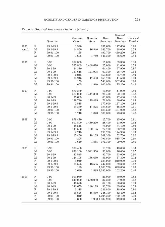
While tax payers file on an individual basis in Canada, the LAD alsomatches individuals with their partners using a variety of matching criteria.The samples upon which Table 4 are based include individuals in the same agegroup as above, and the mean spousal earnings figures are for those spouseswho have some minimal connection with the labour market – in this case weset a minimum earnings level of $1,000 for a spouse to be defined to haveearnings.

The final two columns in Table 4 indicate that spousal earnings patternsare very asymmetric in the top fractiles. Women in the top 0.1 per cent havehusbands with positive earnings in about 90 per cent of cases, and this



Table 4: Spousal Earnings Patterns

SpousalQuantile Quantile Mean Mean Per Cent

Quantile Count Sum Earnings Earnings Positive

1983 F 0-90 789,500 7,300 25,500 0.88M 0-90 389,420 1,178,920 16,600 12,400 0.36F 90.1-99 14,305 38,300 39,300 0.87M 90.1-99 92,500 106805 40,200 15,200 0.19F 99.1-99.9 740 77,800 105,700 0.89M 99.1-99.9 9,530 10,270 79,100 19,100 0.06F 99.91-100 75 220,200 180,900 0.87M 99.91-100 12,05 1,280 234,300 32,500 0.28

1985 F 0-90 776,520 8,600 28,600 0.88M 0-90 409,275 1,185,795 18,700 13,600 0.45F 90.1-99 14,965 42,800 44,800 0.86M 90.1-99 99,010 1,139,75 44,600 16,700 0.30F 99.1-99.9 915 87,800 108,600 0.83M 99.1-99.9 10,410 11,325 89,100 21,700 0.23F 99.91-100 80 291,100 410,100 0.81M 99.91-100 1,300 1,380 277,800 38,400 0.36

1987 F 0-90 799,920 10,100 31,300 0.88M 0-90 448,145 1,248,065 20,800 15,000 0.54F 90.1-99 18,490 47,300 51,600 0.88M 90.1-99 111,135 129,625 49,200 18,900 0.45F 99.1-99.9 1,265 99,600 126,700 0.86M 99.1-99.9 11,685 12,950 101,800 25,900 0.39F 99.91-100 105 254,000 232,000 0.81M 99.91-100 1,410 1,515 339,500 46,600 0.46

1989 F 0-90 842,060 12,200 35,400 0.87M 0-90 516,380 1,358,440 23,900 17,000 0.60F 90.1-99 21,330 55,300 65,300 0.90M 90.1-99 128,640 149,970 57,200 22,100 0.56F 99.1-99.9 1,515 129,000 153,200 0.89M 99.1-99.9 13,595 15,110 133,900 32,100 0.51F 99.91-100 145 433,900 815,700 0.93M 99.91-100 1,590 1,735 602,300 68,700 0.52

1991 F 0-90 818,335 13,500 36,700 0.83M 0-90 520,745 1,339,080 23,800 18,900 0.58F 90.1-99 27,840 59,200 64,200 0.88M 90.1-99 129,390 157,230 61,800 25,500 0.60F 99.1-99.9 1,670 131,600 139,700 0.89M 99.1-99.9 14,035 15,705 136,900 34,900 0.52F 99.91-100 130 422,300 472,700 0.92M 99.91-100 1,620 1,750 491,500 61,600 0.50

1993 F 0-90 84,5825 14,200 37,400 0.80M 0-90 54,7790 1,393,615 24,000 20,200 0.55F 90.1-99 34040 61700 62900 0.87M 90.1-99 133635 167675 64200 27600 0.62


Table 4: Spousal Earnings Patterns (contd.)

SpousalQuantile Quantile Mean Mean Per Cent

Quantile Count Sum Earnings Earnings Positive

1993 F 99.1-99.9 1,990 137,600 147,600 0.90contd. M 99.1-99.9 14,850 16,840 143,700 38,000 0.55

F 99.91-100 135 490,700 430,200 0.89M 99.91-100 1,605 1,740 546,300 66,600 0.44

1995 F 0-90 852,805 15,000 39,300 0.80M 0-90 555,805 1,408,610 25,000 21,000 0.55F 90.1-99 34,380 64,400 67,900 0.87M 90.1-99 137,615 171,995 67,300 28,700 0.64F 99.1-99.9 2,245 150,800 155,700 0.89M 99.1-99.9 15,245 17,490 158,700 41,500 0.59F 99.91-100 155 548,800 502,600 0.90M 99.91-100 1,655 1,810 600,800 75,200 0.44

1997 F 0-90 870,380 16,000 41,900 0.80M 0-90 577,000 1,447,380 26,400 22,100 0.58F 90.1-99 35,635 68,800 77,400 0.88M 90.1-99 139,780 175,415 71,900 30,600 0.65F 99.1-99.9 2,515 177,600 157,100 0.89M 99.1-99.9 15,360 17,875 185,600 46,800 0.61F 99.91-100 160 683,500 431,000 0.88M 99.91-100 1,710 1,870 800,800 78,600 0.48

1999 F 0-90 878,470 17,700 45,000 0.81M 0-90 601,800 1,480,270 28,400 23,900 0.62F 90.1-99 38,545 74,900 84,100 0.89M 90.1-99 141,560 180,105 77,700 33,700 0.69F 99.1-99.9 2,715 199,700 174,900 0.89M 99.1-99.9 15,450 18,165 209,300 52,700 0.62F 99.91-100 205 791,800 535,700 0.90M 99.91-100 1,640 1,845 971,300 99,000 0.46

2001 F 0-90 903,460 19,700 48,800 0.83M 0-90 638,100 1,541,560 30,800 26,000 0.67F 90.1-99 42,545 82,700 93,000 0.90M 90.1-99 144,105 186,650 86,000 37,300 0.72F 99.1-99.9 3,040 233,900 210,000 0.90M 99.1-99.9 15,525 18,565 242,000 59,600 0.62F 99.91-100 195 1,008,700 698,800 0.90M 99.91-100 1,690 1,885 1,180,000 102,200 0.46

2003 F 0-90 903,980 21,000 50,900 0.83M 0-90 649,000 1,552,980 32,300 27,900 0.68F 90.1-99 46,520 87,100 90,600 0.89M 90.1-99 143,655 190,175 90,700 39,800 0.73F 99.1-99.9 3,315 236,800 188,900 0.90M 99.1-99.9 15,525 18,840 248,100 62,400 0.62F 99.91-100 240 1,028,300 730,100 0.90M 99.91-100 1,660 1,900 1,132,900 119,000 0.43

number is relatively constant throughout the sample period. In contrast, menhave wives with positive earnings in about 50 per cent of cases in the modernera, and a somewhat lower percentage in the early eighties.

These patterns are broadly similar to those in the remainder of the toppercentile, though in the latter case a higher number of female spouses havepositive earnings – about 60 per cent rather than 50 per cent. But the figurefor male spouses in this fractile is similar to the male figure recorded in thetop 0.1 per cent. The first part of the conventional wisdom is therefore borneout by these data.

The actual earnings data indicate that the asymmetry between men andwomen is much more severe at the top compared with the asymmetry in theparticipation rates. Women in the top 0.1 per cent of the distribution havepartners who earn about 70 per cent of the female earnings in the most recentperiod, and about 100 per cent of female earnings in the eighties. For example,in 2003 the top 0.1 per cent of women earned just in excess of one milliondollars while their partners earned about $730,000. In contrast, men in the top0.1 per cent have spouses who, when in the labour market, earn about one-tenth of the male figure. For example, in 2003 the respective figures were$1.13m and $119,000.

The asymmetry is slightly less severe for the remaining part of the topcentile – men have spouses who earn about one-fifth of male earnings whenworking. What these earnings figures indicate about hours of work, this database does not allow us to ascertain, even if it is recognised that labour supplydecisions within the household are made jointly. Nor does our data base haveany information on educational attainment, which is one marker of the degreeof ‘assortative mating’ in the population.

3.4 The Post ‘Tech Bust’ EraAs a postscript to this analysis it is worth noting that the earnings shares

of the top fractiles have not declined in the post-2000 era. If the growing shareof the top one thousandth of the distribution is being driven by the earningspatterns of individuals working in corporations, the tech-bust of 2000 has not had a perceptible impact on this growth. In addition, like Saez and Veall,we have investigated the ‘permanent’ incomes of those at the top by takingthree-year moving averages of earnings. Gottschalk and Moffitt (1994)proposed that some of the increase in US inequality in the modern era isattributable to a greater variance in transitory incomes. However, such anaveraging has virtually no impact on the share growth at the very top for thewhole period that we have examined, nor does it have any impact in the post-2000 era.


IV CONCLUSIONS

This paper investigates some of the socio-economic characteristics of thenew class of Canadian ‘super earners’ that has emerged in the last twodecades. Virtually all other English-speaking economies, including Ireland,have also witnessed the emergence of a top group whose incomes haveincreased dramatically. We have been fortunate to have at our disposal a database of about eighty million tax filers that has yielded large reliable samplesat the very extremity of the earnings distribution. Our principal findings are:first, the top one thousandth of the distribution comes disproportionately fromthe top decile of the parental distribution, whereas the remaining componentof the top centile is considerably more likely to have its origins in the parentaldeciles below the top. Second, women have a low, but increasing, rate ofparticipation in the very top tail; they now form about 10 per cent of the group,as opposed to 5 per cent in the early eighties. In contrast, the earnings ofwomen in this group are not so different from male earnings. Third, there is avery severe asymmetry in the earnings patterns of male and female spouses.About half of top male earners have working partners, whereas about 90 percent of top female earners have working partners. Furthermore, the earningsof ‘secondary males’ are between five and ten times the earnings of ‘secondaryfemales’ in the top 0.1 per cent of the distribution. Fourth, the concentrationof earnings at the top tail is not attributable to any growth in the transitorycomponent of earnings, nor was there any break in this pattern with the ‘techbust’ of 2000.

All data bases have limitations, and the LAD is no exception. While it isrich in the income dimension it has no information on human capital oroccupation. This clearly limits the inferences that can be drawn from it. Inaddition, it is clear that we cannot say if these patterns that we haveestablished for Canada are mirrored in the US, the UK, New Zealand,Australia or Ireland. But they represent a step in filling some of the holes inour knowledge of the characteristics of those individuals and households whoinhabit the very top tail of the earnings distribution in Canada.

REFERENCES

ALBRECHT, J., A. BJORKLAND and S. VROMAN, 2003. “Is There a Glass Ceiling inSweden?” Journal of Labor Economics, Vol. 21, No. 1, pp. 145-177.

ALESINA, A., R. BAQIR and W. EASTERLY, 1999. “Public Goods and EthnicDivisions”, Quarterly Journal of Economics, Vol. 114, pp. 1243-1284.

ALVAREDO, F., E. SAEZ, 2005. “Income and Wealth Concentration in Spain in aHistorical and Fiscal Perspective”, Working Paper, Department of Economics,


University of California at Berkeley, September.ATKINSON, A., 2005. “Top Incomes in the United Kingdom over the Twentieth

Century”, Journal of the Royal Statistical Society, Series A, Part 2, pp. 325-343.ATKINSON, A., F. BOURGUIGNON and C. MORRISON, 1992. Empirical Studies of

Earnings Mobility, Switzerland: Harwood Academic Publishers.ATKINSON, A. and A. LEIGH, 2004. “Understanding the Distribution of Top Incomes

in Anglo-Saxon Countries over the Twentieth Century”, Department of Economics,Australian National University, November.

ATKINSON, A. and W. SALVERDA, 2005. “Top Incomes in the Netherlands and theUK in the Twentieth Century”, Journal of the European Economic Association, Vol. 3, pp. 883-913.

BANERJEE, A. and T. PIKETTY, 2003. “Top Indian Incomes, 1922-2000”, CEPRDiscussion Paper, # 4632, 2003.

BUCHINSKY, M. and J. HUNT, 1999. “Wage Mobility in the United States”, Review ofEconomics and Statistics, Vol. 81, No. 3, pp. 351-368.

CORAK, M., 2004. “Do Poor Children Become Poor Adults? Lessons for Public Policyfrom a Cross Country Comparison of Generational Earnings Mobility”, DiscussionPaper, UNICEF Innocenti Research Centre, Florence, Italy, September .

CORAK, M. and A. HEISZ, 1999. “The Intergenerational Earnings and IncomeMobility of Canadian Men: Evidence from Longitudinal Income Tax Data”, Journalof Human Resources, Vol. 34, pp. 504-533.

DELL, F., T. PIKETTY and E. SAEZ, 2005. “Income and Wealth Concentration inSwitzerland over the 20th Century”, CEPR Discussion Paper 5090, May.

DIAMOND, J., 2005. “Collapse. How Societies Choose to Fail or Succeed”, New York:Viking Press.

DUCLOS, J.Y., J. ESTEBAN and D. RAY, 2004. “Polarisation: Concepts, Measurement,Estimation”, Econometrica, Vol. 72, pp. 1737-1772.

ECKSTEIN, Z. and E. NAGYPAL, 2002. “The Evolution of U.S. Earnings Inequality:1961-2002”, Federal Reserve Bank of Minneapolis, Quarterly Review, December.

FAJNZYLBER, P., D. LEDERMAN and N. LOAYZA, 2002. “Inequality and Crime”,Journal of Law and Economics, Vol 45, No. 1.

FELDSTEIN, M., 1995. “The Effect of Marginal Tax Rates on Taxable Income: A PanelStudy of the 1986 Tax Reform Act”, Journal of Political Economy, Vol. 103, No. 3,pp. 551-572.

FOSTER, J., J. GREER and E. THORBECKE, 1984. “A Class of Decomposable PovertyMeasures”, Econometrica, Vol. 52, No. 3, pp. 761-766.

GLAESER, E., 2005. “Inequality”, Harvard Institute of Economic Research, DiscussionPaper Number 2078, July.

GOTTSCHALK, P. and R. MOFFITT, 1994. “The Growth of Earnings Instability in theUS Labor Market”, Brookings Papers on Economic Activity, pp. 217-272.

GRAWE, N., forthcoming, 2006. “The Extent of Lifecycle Bias in Estimates ofIntergenerational Earnings Persistence”, Labour Economics.

KENNICKELL, A., 2001. “An Examination of Changes in the Distribution of Wealthfrom 1989 to 1998: Evidence from the Survey of Consumer Finances”, WorkingPaper, Washington: Federal Board.

MORIGUCHI, C. and E. SAEZ, 2005. “The Evolution of Income Concentration inJapan, 1885-2002: Evidence from Tax Statistics”, Working Paper, Department ofEconomics, University of California at Berkeley.


NOLAN, B., 2006. “Long-Term Trends in Top Income Shares in Ireland”, in A. B.Atkinson and T. Piketty (eds.), Top Incomes over the Twentieth Century, Oxford:Oxford University Press.

PIKETTY, T., 2003. “Income Inequality in France, 1901-1998”, Journal of PoliticalEconomy, Vol. 111, No. 5, pp. 1004-1042.

PIKETTY, T. and E. SAEZ, 2003. “Income Inequality in the United States, 1913-1998”,Quarterly Journal of Economics, Vol. 118, No. 1, pp. 1-39.

SALA-I-MARTIN, X., 2002. “The World Distribution of Income”, Columbia University,Economics Department Working Paper, April.

SAEZ, E. and M. VEALL, 2005. “The Evolution of High Incomes in Northern America:Lessons from Canadian Evidence”, American Economic Review, Vol. 95, No. 3, pp.831-849.

SEN, A., 1976. “Poverty an Ordinal Approach to Measurement”, Econometrica, Vol. 44,pp. 219-231.

SHORROCKS, A., 1995. “Revisiting the Sen Poverty Index”, Econometrica, Vol. 63, pp.1225-1230.

SOLON, G., 1992. “Intergenerational Income Mobility in the United States”, AmericanEconomic Review, Vol. 82, pp. 393-408.

SOLON, G., 1989. “Biases in the Estimation of Intergenerational EarningsCorrelations”, Review of Economics and Statistics, Vol. 71, pp. 172-174.


mobility and gender at the top tail of the earnings

Documents