mobilisation of soil-bound dioxins at an old sawmill...
TRANSCRIPT

Mobilisation of soil-bound dioxins at an old sawmill area.
Impact of excavation on groundwater levels of PCDF/PCDDs at Norrbyskär.
Daniel Larsson
Daniel Larsson
Master Thesis 45 ECTS
Report passed: 12th of July 2016
Supervisor: Staffan Lundstedt
Examiner: Erik Björn


Abstract
High concentrations of polychlorinated dibenzofurans (PCDFs) and polychlorinated
dibenzo-p-dioxins (PCDDs) can be found in the soil at the old industrial sawmill area
on the island group Norrbyskär, Sweden. These persistent organic pollutants are
found as a consequence of historical use of chlorophenol based preservatives that
were used to treat freshly sawn goods. As remediation through excavation has been
suggested for the site, the present project was launched in order to assess the risk of
mobilisation of PCDF/PCDDs via groundwater during such an excavation. A small
scale excavation was carried out upgradient of two groundwater wells termed GW100
and GVR1. Groundwater samples were acquired for five different time points (one
prior and four after excavation) and subsequently analysed with gas chromatography
coupled with high resolution mass spectrometry. Furthermore, soil and wood
samples from the site were analysed and compared to the groundwater samples. The
results of the analysis showed that the excavation caused a significant increase in
GW100 groundwater PCDF/PCDD levels. It was also argued that such an increase
should be present for GVR1 as well, but in between the analysed time points.
Homologue profiles were the same for groundwater, wood and soil samples
suggesting a common source of contamination, which was suggested to be a 2,3,4,6-
tetrachlorophenol based preservative. Furthermore, the main mode for mobilisation
was suggested to be via soil colloids for GW100 and via dissolved organic carbon for
GVR1 groundwater.

II

III
List of abbreviations
Dioxins:
PCDFs polychlorinated dibenzofurans
PCDDs polychlorinated dibenzo-p-dioxins
TCDFs tetrachlorinated dibenzofurans
PeCDFs pentachlorinated dibenzofurans
HxCDFs hexachlorinated dibenzofurans
HpCDFs heptachlorinated dibenzofurans
OCDF octachlorinated dibenzofuran
TCDDs tetrachlorinated dibenzo-p-dioxins
PeCDDs pentachlorinated dibenzo-p-dioxins
HxCDDs hexachlorinated dibenzo-p-dioxins
HpCDDs heptachlorinated dibenzo-p-dioxins
OCDD octachlorinated dibenzo-p-dioxin
Other abbreviations:
ASE Accelerated Solvent Extractor
DOC dissolved organic carbon
DOM dissolved organic matter
GC gas chromatography
GC-HRMS gas chromatography high resolution mass spectrometry
IS internal standard
IUPAC International Union of Pure and Applied Chemistry
Kow n-octanol-water partitioning coefficient
Kpw sediment (particle)-water partitioning coefficient
LOI loss-on-ignition
MQ water Milli-Q water
OM organic matter
POM particulate organic matter
POPs persistent organic pollutants
QS quantification standard
RS recovery standard
SPE discs solid phase extraction discs
TEFs toxic equivalence factors
TEQ toxic equivalent
WHO World Health Organisation
WHO-TEFs World Health Organisation toxic equivalence factors
WHO-TEQs World Health Organisation toxic equivalents
WHO-TEQ LB World Health Organisation toxic equivalents lower bound

IV

V
Table of contents
Abstract .......................................................................................................................... I
List of abbreviations ................................................................................................... III
Table of contents .......................................................................................................... V
1. Popular scientific summary including social and ethical aspects .............................. 1
1.1 Popular scientific summary .................................................................................. 1
1.2 Social and ethical aspects .....................................................................................2
2. Introduction ...............................................................................................................3
2.1 Norrbyskär ...........................................................................................................3
2.2 Dioxins – toxic and persistent organic pollutants .............................................. 4
2.3 Organisation of the project .................................................................................. 5
2.4 Aim of the diploma work ..................................................................................... 5
3. Experimental ............................................................................................................ 6
3.1 Excavation and soil sampling.............................................................................. 6
3.2 Groundwater sampling method and materials .................................................. 6
3.2.1 Pumped groundwater samples .................................................................... 6
3.2.2 Bailer samples .............................................................................................. 6
3.3 Dioxin analysis .................................................................................................... 6
3.3.1 Consumables and materials ......................................................................... 6
3.3.2 Filtration of groundwater samples ............................................................... 7
3.3.3 Soil and wood work-up prior to extraction.................................................. 8
3.3.4 Extraction of samples .................................................................................. 8
3.3.5 Sample clean-up prior to GC-HRMS analysis ............................................. 9
3.3.6 Gas chromatography coupled with high resolution mass spectrometry
(GC-HRMS) .......................................................................................................... 9
3.3.7 Quantification of 2,3,7,8-substituted PCDF/PCDDs .................................. 10
3.4 Additional analyses ............................................................................................ 10
3.4.1 Loss-on-ignition .......................................................................................... 10
3.4.2 Analyses performed by ALcontrol .............................................................. 10
4. Results and Discussion ............................................................................................ 11
4.1 Impact of the upgradient excavation ................................................................. 11
4.1.1 Impact on GW100 groundwater .................................................................. 11
4.1.2 Impact on GVR1 groundwater .................................................................... 12
4.1.3 Comparison between GW100 and GVR1 .................................................... 14
4.2 Dioxin distribution in the particulate and dissolved phase .............................. 14
4.3 Comparison between the conventional bailer sampling method and the low-
flow pumping method utilized in this study ............................................................ 15
4.4 Dioxin concentrations in soil and woodchips ................................................... 16
4.5 Homologue profile comparison ......................................................................... 17
4.6 Quality control of the analytical results ............................................................. 19
4.6.1 Laboratory blanks ....................................................................................... 19
4.6.2 Determination of PCDF/PCDD concentrations in a reference material ... 20
4.7 Additional analyses ............................................................................................ 21
4.8 Mobilisation of 2,3,7,8-PCDF/PCDDs ............................................................. 23
5. Conclusions .............................................................................................................. 27
6. Outlook ................................................................................................................... 28

VI
7. Acknowledgements ................................................................................................. 29
8. Appendix ................................................................................................................. 30
8.1 Derivation of the formula used for quantification of dioxins ........................... 30
8.2 Additional Tables and Figures .......................................................................... 32
9. References ................................................................................................................ 45

1
1. Popular scientific summary including social and
ethical aspects
1.1 Popular scientific summary
Today the island group of Norrbyskär outside of Umeå, Sweden, is a popular
attraction for nature-loving tourists. Tens of thousands of people visit the islands
every year. In addition to the bountiful nature found there, the islands have a
fascinating history. Between the years of 1895 and 1952, one of Europe’s largest
sawmills was operational at Norrbyskär. The entirety of Norrbyskär was dedicated to
this industry and workers and their families lived on the islands. In fact, an entire
functional community was formed, with schools for the young and every necessity
available – all centred around the sawmill industry.
Sawn goods, such as planks, are often treated with chemicals in order to prolong
their “lifetime”. This process is referred to as impregnation. At Norrbyskär the
freshly sawn goods were sprayed with preservatives in order to prevent decay and
discoloration. Unfortunately, the preservatives they used also contained toxic by-
products that are termed dioxins. Dioxins are regarded as “persistent organic
pollutants” and can still be found in soil at Norrbyskär to this date.
Since Norrbyskär is frequently visited by tourists and also have a number of
domiciled inhabitants parts of the year, it has been suggested that the toxic soil
should be dug up and moved somewhere safer. However, there is a concern that such
digging will cause a significant part of the dioxins to end up in the groundwater and
then transported out into the ocean and areas adjacent to the contaminated sites.
Therefore, this study was initiated to assess the risk of dioxins ending up in the
groundwater during the suggested excavation processes.
Trenches were dug upstream of tw0 groundwater wells, and changes in dioxin levels
in the groundwater was studied. Groundwater samples were acquired both before,
and then 2, 7, 15 and 56 days and after the excavation. Soil samples and wood from
the site was also collected during the excavation and was compared to the
groundwater samples.
The results of the study show that a noticeable increase of dioxins was detected in
one of the groundwater wells about a week after the digging. The present study also
argues that a similar effect likely took place in the other groundwater well. Based on
the “chemical fingerprints” found in all the samples, the commercial mixture of
preservative most likely used at Norrbyskär around a century ago was identified. In
one of the groundwater wells the mode of transport of dioxins was suggested to be
via colloids, which are small particles that remain suspended in a liquid due to their
small size (similar to the fat in a glass of milk). For the other groundwater well the
mode of transport was suggested to be similar in the way that it was facilitated by
“carriers”, but different in the way that the carriers were smaller and by definition
dissolved – i.e. the dioxins were likely transported via dissolved organic carbon
(DOC). DOC is defined as organic carbon that is sufficiently small to pass through a
filter of a given pore size, and often consists of a vast number of chemicals that are
hard to define.

2
In conclusion a significant effect, in terms of increased dioxin levels in the
groundwater, was noted as a result of the excavation, and thus care should be taken
to prevent such “leakage” of dioxins when large-scale excavation takes place at
Norrbyskär.
1.2 Social and ethical aspects
Even though only low (if any) concentrations of the most toxic tetra- and penta
chlorinated PCDF/PCDDs were found at Norrbyskär, all of the 2,3,7,8-substituted
PCDF/PCDD congeners are toxic to humans and wildlife. Indeed the main reason for
the suggested remediation process is the risk associated with these compounds.
A very important question is which scenario that poses the greatest risk to humans
and the environment – remediation or letting the pollutants remain in the soil? This
constitutes an ethical dilemma. The present study showed that an excavation process
will cause mobilisation of dioxins via the groundwater. In addition, previous studies
have shown limited levels of soil-bound dioxins on the surrounding areas and
wildlife. The author suggests that very careful risk assessment is performed prior to
any remediation activities. Perhaps it is safer to leave the dioxins where they are? It
should also be noted that the remediation is of interest from a financial point of view
as the cost of a remediation process may reach and even exceed 100 million SEK,
which perhaps could be put to better use.
The fact that the present study caused mobilisation of dioxins in the environment
could be regarded as unethical. However, compared to excavation of the entire
contaminated area this mobilisation should be small and may provide information
that can aid in prevention of a large-scale mobilisation of dioxins during the coming
remediation. Indeed, this study was performed with permission from Umeå
Municipality in order to aid with risk assessment of the site. Therefore the actions
taken should be justified.
As for laboratory work, great care was taken to dispose of chemicals and
contaminated materials in a correct fashion. Soil and wood spilled in the fume hoods
was wiped up and disposed as hazardous waste. All laboratory equipment in contact
with samples were rinsed with first acetone and then toluene (where applicable) in
order to both account for the majority of the sample in the analysis as well as prevent
chemicals from ending up in the environment or contaminating future laboratory
analyses. However, it is unlikely that all of the dioxins were accounted for, and
cleaning of laboratory equipment in the dishwasher may have caused some of the
dioxins to end up in the drain water. This fraction should be very small, however, and
should have negligible effect on the environment. It should also be noted that large
amounts of solvents were used for the laboratory analyses. Thus the methodology
cannot be considered “Green”, even if the solvents were disposed of correctly.

3
2. Introduction
2.1 Norrbyskär
The picturesque island group Norrbyskär is situated approximately 40 km south of
the city of Umeå, Sweden, and approximately 2.5 km from the mainland. The islands
are only accessible by ferry – however, this fact do not deter tens of thousands of
visitors every year1. A large part of the islands’ unique atmosphere is accounted for by
the blend of bountiful nature and the ruins of an old sawmill industry.
One of Europe’s largest sawmill industries was operational at Norrbyskär between
the years 1895 and 1952, and at the peak of production, around 1920, it produced
approximately 95 000 m3 sawn goods per year. Figure 1 shows an aerial photograph
of the sawmill industry at Norrbyskär taken around 1930. In order to prevent
spoilage of the sawn goods by Ophiostomatales fungi they were sprayed with
chlorophenol preservatives1. Old records have shown that a commonly used
chlorophenol-based preservative named “Dowicide” was used at Norrbyskär2.
Figure 1. Aerial photograph of the sawmill industry at Norrbyskär taken around
1930. The actual sawmill can be seen at the tip of the middle island. Picture from
MoDo's picture archive, Holmen AB. Reproduced with permission from Norstedt, S
(2016).
Today, it is known that chlorophenol preservatives contained high molecular weight
chlorinated impurities in the form of polychlorinated dibenzo-p-dioxins (PCDDs)
and polychlorinated dibenzofurans (PCDFs)3,4. Indeed, very high levels of
PCDF/PCDDs have been found in the soil at plank-yards, and (especially) at the
sawmill-area at Norrbyskär1. Possible reasons for the soil contamination are that the
sawn goods dripped contaminated preservative onto the ground and that dried wood
was planed/dressed2 thus forming contaminated wood-shavings. Chlorophenols,
however, were only found below site-specific threshold values in a main study
performed by Tyréns AB1, which is likely attributed to relatively high water solubility
and short half-lives of these compounds5.

4
2.2 Dioxins – toxic and persistent organic pollutants
The name “dioxins” is commonly used to refer to a class of polychlorinated aromatic
hydrocarbon compounds with similar structure and chemical behaviour6. Two sub-
groups of chemicals are commonly included in this class, namely the PCDDs and
PCDFs7. Some authors also include the “dioxin-like” polychlorinated biphenyls
(PCBs)6, but they are disregarded in this study. In terms of PCDDs and PCDFs,
“polychlorinated” often refers to tetra- to octachlorinated compounds (even though
dioxins also can be mono- to trichlorinated), which can be divided into “homologue
groups”, namely: tetra- (TCDDs), penta- (PeCDDs), hexa- (HxCDDs), hepta-
(HpCDDs) and octachlorinated dibenzo-p-dioxin (OCDD) for PCDDs and tetra-
(TCDFs), penta- (PeCDFs), hexa-(HxCDFs), hepta- (HpCDFs) and octachlorinated
dibenzofuran (OCDF) for PCDFs8. Each of these homologue groups consists of a
given number of congeners, i.e. specific chemical compounds. In total, 136 tetra-
octachlorinated congeners exist8. However, only seven PCDFs and 10 PCDDs are
considered to have dioxin-like toxicity6,7. These 17 congeners are commonly found in
literature under the name of 2,3,7,8-substituted congeners8,9, as they all are
substituted at positions 2, 3, 7 and 8. The numbering used in the nomenclature for
PCDFs and PCDDs is illustrated in Figure 2. As an example, the PCDD congener with
chlorine substitutions at location 2, 3, 7 and 8 is called 2,3,7,8-tetrachlorinated
dibenzo-p-dioxin (2,3,7,8-TCDD).
Figure 2. Numbering used for naming dioxins based on the positions where hydrogen
atoms may be substituted with chlorine atoms in a) PCDFs and b) PCDDs6.
Chemical and physical properties of dioxins vary according to the degree of chlorine
substitutions6, for example; aqueous solubility10–12 and liquid vapour pressure11–13
decrease with an increased degree of chlorination, while the n-octanol-water
partitioning coefficient (Kow)11–13, the sediment (particle)-water partitioning
coefficient (Kpw)13 and molar volume11 increase with increasing degree of
chlorination.
Dioxins are considered one of the most important classes of persistent organic
pollutants (POPs) as they are highly persistent in nature, particularly in soil and
sediments, and in adipose tissues in animals. They partition strongly to organic
matter (OM) in soils and “avoid” aqueous phases14. Suggested degradation half-lived
can be found in an article by Sinkonnen and Paasivirta15, where the shortest
degradation half-life of chosen PCDF/PCDDs in soil is approximately 17 years, and
the longest approximately 274 years. Dioxins in nature (biota and environment) are
found in complex mixtures of PCDF/PCDD congeners with concentrations that vary
between trophic levels16.
Abel and Haarmann-Stemmann17 refer to 2,3,7,8-TCDD as “the most potent man-
made toxicant that can cause teratogenesis, tumor promotion, endocrine disruption,

5
immune and liver toxicity, as well as distinctive skin disorders (chloracne)”. The
toxicological mechanism is mediated via the aryl hydrocarbon receptor, which is a
ligand-activated transcription factor located in the cytosol17,18. There appears to be
some controversy regarding the exact mechanism as three different papers, spanning
over three years, differ in the proposed mechanisms17–19.
In terms of risk assessment, the complexity of dioxin distribution in natural systems
is addressed by means of Toxic Equivalence Factors (TEFs). As dioxin toxicity is
mediated via the same toxicological mechanism, toxic PCDF/PCDD concentrations
are given relative to the most toxic congener, 2,3,7,8-TCDD. 2,3,7,8-TCDD is given a
TEF of 1, and as an example, 1,2,3,4,7,8-HxCDD which only is 10% as toxic, is given a
TEF of 0.16,16,20. The overall toxic equivalent (TEQ) concentration is determined by
the following formula16,20:
∑ ∑ ∑
Please note that the “dioxin-like” PCBs are excluded from this equation in the
present study.
In the year 1997, consensus toxic equivalency factors were re-evaluated by an
initiative from the World Health Organisation (WHO). These TEFs are referred to as
WHO-TEFs and are found in the review by Van den Berg et al.16. The newest version
of these TEFs, from 2005, are used in this paper21.
2.3 Organisation of the project
This project has been performed as a part of a development project that is run in
parallel to the planning of the remediation of the contaminated areas on
Norrbyskär22. The project stems from a main study performed by Tyréns AB on
behalf of Umeå Municipality1, in which it was suggested that the soil at the site
should, at least partly, be remediated through excavation. Following this suggestion,
in conjunction with previous experiences from other studies, the present project was
initiated.
2.4 Aim of the diploma work
The overall aim of this project was to study the impact of excavation, which will take
place during the coming site remediation, on the mobilisation of dioxins in the soil at
the highly contaminated saw mill area at Norrbyskär.
The specific objectives were:
• To measure whether the dioxin levels in groundwater downgradient of
excavation points change as a result of a mobilisation process.
• To determine how the dioxins in the groundwater are distributed between the
particulate and the dissolved phase, including both the freely dissolved
molecules and the fraction associated with dissolved organic carbon (DOC),
and how this affects the mobilization.
• To compare homologue profiles for groundwater and upgradient soil.
• To correlate dioxin levels with relevant chemical properties in order to
explain their leaching behaviour.
• To compare a pumped, low flow sampling method with a more traditional
bailer based method.

6
3. Experimental
3.1 Excavation and soil sampling
An excavator was hired by Umeå municipality 08-09-2015. Trenches were dug five
meter upgradient of the two groundwater wells to be used in this study. The
dimensions of the trenches were approximately 5 x 1 x 2.5 m (length, width and
depth). Groundwater was encountered at approximately 1.5 m depth. Soil samples
were collected from excavated masses, into gas tight bags, during the excavation and
from two depth intervals, i.e. 0-1 m and 1-2 m and put in an icebox during transport.
After 1-2 hours the soil was put back into the trenches, as the ground was considered
to have been sufficiently disturbed. The soil samples were put in a freezer until
analysis.
3.2 Groundwater sampling method and materials
3.2.1 Pumped groundwater samples
The groundwater samples were acquired from two groundwater wells, termed
GW100 (installed 11-08-2015) and GVR1 (installed 2009) and were sampled just
before the excavation, 2 ,7, 15 and 56 days after excavation. Please note that heavy
rain took place during Day 15. Each sample was pumped alternately into one 1 L glass
bottle and a 250 mL plastic bottle by filling a third of each bottle at the time. This was
done to obtain “identical” water in both bottles. Two of these “double” samples were
collected from both groundwater wells at each sampling occasion. The pumping was
done by an Eijkelkamp 12 Vdc peristaltic pump with an improvised flow-cell and
operated at a low-flow. The pumping rate was between 100 mL and 200 mL per
minute. Prior to sampling, the groundwater was pumped at low flow until steady
state was reached. Steady state was assayed by measuring indicator parameters,
namely: pH, oxidation-reduction potential, percentage of dissolved oxygen,
conductivity, total dissolved solids and temperature, utilizing a Hanna Instruments
HI-9828 Multi-Parameter Water Quality Portable Meter. Several studies have shown
this pumping method to produce representative samples with low variability23–25.
Subsequent to sampling, the samples were stored cold in an icebox during transport.
The plastic bottles were delivered to ALcontrol for analysis of DOC and suspended
substances, while the glass bottles were brought to the Environmental Chemistry
Laboratory at Umeå University, put in a laboratory fridge until the next day, when
they were filtered and analysed as a part of this study. Samples were termed
“groundwater well”-“sample number” “Sample date”, e.g. GVR1-1 150915.
3.2.2 Bailer samples
In order to investigate differences between sampling techniques two bailer samples
were taken 15 days after excavation after the pumped samples had been acquired.
Bailer samples were only acquired for GW100. With the exception of the sampling
method and an additional type of filter (below), the bailer samples were treated the
same way as the other groundwater samples.
3.3 Dioxin analysis
3.3.1 Consumables and materials
This section will list and summarize the consumable materials of the experimental
section. The context in which they were used is found in the coming sections of 3.3.

7
0.45 µm polyamide filters: Sartorius Stedim Biotech. Solid phase extraction (SPE)
discs: ENVI-DISC™, SUPELCO Analytical. Glass Microfiber filters: GF/B, GE
Healthcare Life Sciences, Whatman™. 30 mm cellulose filters: Dionex Corporation.
“Hydromatrix”: Thermo Scientific™ Dionex™ ASE™ Prep DE (inert diatomaceous
earth). Na2CO3: Sodium Carbonate, anhydrous for analysis, Merck KGaA. Na2SO4:
Sodium Sulphate, anhydrous GR for analysis, Merck KGaA. Neutral silica: Silica gel
60 (0.063-0.200 mm) for column chromatography, Merck KGaA. Activated carbon:
AX21, Anderson Development Co., Adrian, MI, USA. Celite: Silicagel Celpure, Celite
® 545, Sigma Aldrich. Gas chromatography (GC)-vials: 1.5 mL, VWR. GC-vial
inserts: Micro-Insert 0.1 mL, VWR. KOH pellets: AnalR NORMAPUR pellets, VWR.
Methanol: HPLC grade Fisher Scientific. Concentrated HCL: 37% AnalR
NORMAPUR, VWR. Toluene: AnalR NORMAPUR, VWR. Acetone: HPLC grade,
Fisher Scientific. Tetradecane: analytical standard, Fluka Analytical.
Dichloromethane: Analytical reagent grade, Fisher Scientific. H2SO4: 95-97% for
Analysis, Merck KGaA. n-Hexane: CHROMASOLV® for HPLC, ≥97.0% (GC), Sigma-
Aldrich.
Activated silica was prepared by first purifying silica gel in an oven at 550° C for 24 h,
then storing it at 130° C for at least 1 day prior to use. KOH-silica was prepared from
168 g KOH pellets, 800 mL methanol, and 300 g silica gel, mixed at 55 °C for 90 min,
and cleaned with 2 x volume methanol and 2x volume dichloromethane and
subsequently dried at room temperature. 40 % H2SO4-silica was prepared from 300 g
activated silica gel and 200 g H2SO4. Na2SO4 and Na2Co3 were purified in the same
way as the silica gel. AX21 carbon and Celite were mixed in the following
proportions: 7.9:92.1.
All multi-use glassware was cleaned in a dishwasher followed by a laboratory oven at
550° C, warm-up time: 270 min, heat time: 120 min. All other equipment that was in
contact with the samples was cleaned in a dishwasher and rinsed with first acetone
and then toluene (where applicable).
Internal standards (IS) consisted of 13C-labelled 2,3,7,8-substituted PCDF/PCDDs.
40µL (5.9-12 pg/µL). IS was added to each sample and quantification standard (QS).
Recovery standards (RS) consisted of 13C-labelled PCDF/PCDDs of 1,2,3,4-TCDD,
1,2,3,4,6-PeCDF, 1,2,3,4,6,9-HxCDF and 1,2,3,4,6,8,9-HpCDF. 40 µL RS (15 pg/µL)
was added to each sample and QS just prior to the gas chromatography high
resolution mass spectrometry (GC-HRMS) analysis. The QS consisted of non-labelled
2,3,7,8-substituted PCDF/PCDDs in known amounts (95 – 1001 pg). IS, RS and QS
were used as in Liljelind et al.26.
3.3.2 Filtration of groundwater samples
The groundwater samples were vacuum-filtered the day after sampling, first through
0.45 µm polyamide filters and finally through a SPE disc. The polyamide filters were
used to collect suspended particles (≥0.45 µm in diameter) and the SPE disc to
collect the “dissolved organic phase” (including suspended particles <0.45 µm in
diameter, DOC and freely dissolved compounds). For each batch of samples, one
laboratory blank was analysed, consisting of Milli-Q (MQ) water (18.2 MΩ cm at
25°C, Q-POD®, Millipore). As a general rule, the laboratory blanks were filtered first
(with the exception of the first batch of samples). After each step, the used equipment
was rinsed with first acetone, then toluene and this “rinse” was stored in a glass
bottle in a laboratory fridge.

8
Prior to filtration, the mass of each sample bottle was determined. The groundwater
was then vacuum-filtered through polyamide filters which were collected and stored
in glass petri dishes. After separating the particulate fraction from the rest of the
sample, 6 mL methanol, IS and 25 drops of concentrated HCl were added to the
filtrate. Furthermore, IS was added to a vial of QS for each batch of samples. The SPE
disc was washed with 20 mL toluene, conditioned with 6 mL methanol and 10 mL
MQ water. It was not allowed to run dry, i.e. some water was left prior to application
of the sample. Vacuum-filtration through the SPE disc was then done the same was
as for the polyamide filters. After filtration, the SPE discs were stored with the filters
and moved to the laboratory freezer. Finally, the mass of the empty, rinsed and dry
water bottles was determined such that the sample mass could be calculated.
Selected samples, i.e. GW100-2 150915, GW100-2 031115, GVR1-2 150915 and GVR1-
2 031115, were split in terms of filters and SPE discs, which were individually
analysed in order to determine if the dioxins were mainly present in the particulate
fraction or the dissolved organic fraction.
The bailer samples were filtered and treated in the same way as the pumped samples
with two exceptions; the filtration took place 9 days after sampling and prior to the
filtration they were first filtered through glass microfiber filters as both sample
bottles had notable amounts of soil particles in the bottom.
3.3.3 Soil and wood work-up prior to extraction
The soil samples were picked out of the freezer and dried for 48 hours at room
temperature in large petri dishes, as they were too wet to be sifted. The samples were
then sifted through a 2 mm sieve and stored at room temperature for one day prior to
extraction, as the extraction equipment had to be cleaned overnight (below). Pieces
of wood were picked out in approximately equal amounts from both sample depths
for each trench, mixed together and subsequently shaved/ cut into small pieces with
a scalpel.
3.3.4 Extraction of samples
The extraction was done by an Accelerated Solvent Extractor (ASE) 350 (Dionex
Corporation). Prior to sample extraction, 34 mL stainless steel extraction cells were
assembled with 30 mm cellulose filters, filled with Hydromatrix and washed in the
ASE 350 with toluene at 150° C27, three static cycles of 5 min each; 100% rinse
volume and 60 sec purge time.
Samples were put in the washed cells, surrounded with the washed Hydromatrix and
mounted in the ASE 350. The extraction of all samples was performed with the same
parameters as in the washing step, except for 10 min static times. The extracts were
collected in vessels covered with aluminium foil, which then were stored in a
laboratory fridge until further work-up. The pumped groundwater samples and
corresponding blanks were extracted in three separate batches and the bailer, soil,
wood and reference samples in a fourth batch.
For groundwater samples, filters and SPE discs were put in the same extraction cells,
with the exception of the split samples. For the two bailer samples, the glass
microfiber filters were also included.

9
Two replicates, of approximately 5 g each, were extracted for each soil sample, and
approximately 3 g of each wood sample. The soil blank consisted of Hydromatrix
only. A reference sample, consisting of dried and homogenised sediment previously
analysed at the laboratory and also in an intercalibration study (3rd InterCinD,
2014/15, QA/QC Study)28 was analysed in parallel in order to check the accuracy of
the method used. IS was added to the soil, wood and reference samples in the ASE
cells.
3.3.5 Sample clean-up prior to GC-HRMS analysis
Each extract was transferred to a round bottom flask together with the “rinse” (from
the filtration), and evaporated to approx. 5 mL. Residual water was removed by the
addition of anhydrous Na2CO3. IS was added to the particulate (filter) fractions of
split samples, and the rinse of these samples were then only combined with their
corresponding dissolved (SPE disc) fractions. Each sample was transferred to a pear-
shaped flask using 3 x 5 mL toluene. 100 µL tetradecane was added and the extracts
were evaporated until only tetradecane remained. Multilayer-columns were
prepared: a 16 mm glass column was packed with, in order: 1: glass wool, 2: 3 g
KOH-silica, 3: 1.4 g neutral activated silica, 1,5 g 40 % H2SO4-silica and 3 g Na2SO4.
The column was washed with n-hexane, two times the volume of column contents.
The samples were transferred to columns with approximately 3 x 1 mL n-hexane.
Elution into pear-shaped flasks was made with 100 mL n-hexane. Evaporation of the
samples was performed until 1 mL sample remained. Carbon-celite columns were
prepared: a 10 mL glass column, cut at both ends, was packed with glass wool, 0.5 g
activated carbon mixed with celite, and glass wool. The column was washed with 10
mL dichloromethane/methanol/toluene 15/4/1 (V/V/V), 5 mL dichloromethane/n-
hexane 1/1 (V/V) and 10 mL n-hexane. The samples were transferred to columns
with 3 x 1 mL n-hexane. Unwanted compounds were eluted with 50 mL
dichloromethane/n-hexane 1/1 (V/V). PCDFs and PCDDs were then back-eluted with
40 mL toluene. 40 µL tetradecane was added to the fraction and evaporated in a
small pear-shaped flask until only tetradecane remained. An additional multilayer
column was prepared as above, but in Pasteur pipettes and in smaller amounts: 0.1 g
KOH-silica, 0.1 g activated silica, 0.2 g 40 % H2SO4-silica and 0.1 g Na2SO4. Elution
of the fraction into 12 mL glass vials was made with 8 mL n-hexane. Samples were
stored in a laboratory fridge at this step until the day prior to GC-HRMS analysis.
The day before GC-HRMS analysis the samples and quantification standards were
evaporated by blowing gently with N2 gas. Towards the end of the evaporation RS
was added and evaporation was continued until only tetradecane remained. The
samples and standards were transferred to GC-vials with insert tubes (100 µL).
3.3.6 Gas chromatography coupled with high resolution mass spectrometry
(GC-HRMS)
The GC-HRMS analysis was performed on a Hewlett–Packard 5890 gas
chromatograph (Agilent Technologies) equipped with a DB5MS column (60 m, 0.25
mm, 0.25 µm) and connected to an Autospec Ultima NT 2000D high resolution mass
spectrometer (Waters Corporation) operated in splitless mode. The following
parameters were used: carrier gas: helium - constant flow mode and injection into a
splitless injector at 280 °C. Oven temperature: 190° C for 2 min, followed by an
increase to 278° C – 3.0 °C/min and then to 315° C – 10°C/min, which was held for
4.5 min. The utilised ionisation technique was electron impact. For further details, an
experimental output file from the software can be acquired from the author.

10
3.3.7 Quantification of 2,3,7,8-substituted PCDF/PCDDs
The output files acquired from the GC-HRMS were
visualised in Waters MassLynx™ Software v. 4.1 for
Windows with the ChroTool plugin. The target
compounds were identified by comparing retention
times of selected ions in the mass-spectra of the
samples with those of the QS. Quantification was
performed using the internal standard technique26,
comparing peak areas of the selected ions in the
samples with those in the QS. The equation used for
quantification is found and derived in section 8.1 of the
Appendix. Peak area integration was done with the
following parameters: smoothing (enabled): window
size (scans) – ±3, number of smooths – 2, smoothing
method – mean. ApexTrack (enabled): Peak-to-peak
Baseline Noise – 442 (automatic), Peak Width at 5%
Height (Mins) – 0.227 (automatic), Baseline Start
Threshold% – 0.00, Baseline End Threshold% – 0.50,
Detect shoulders (enabled).
The quantification was done in an accredited excel
sheet provided by the Environmental Chemistry
Laboratory, Department of Chemistry – Umeå
University. In this paper, only the 17 2,3,7,8-
substituted PCDF/PCDDs were quantified
individually. These congeners are summarised in Table
1. WHO-TEQ values were calculated based on the 2005 WHO-TEFs21.
3.4 Additional analyses
3.4.1 Loss-on-ignition
Loss-on ignition (LOI) was performed to estimate the amount of water and organic
material in sifted soil and wood-shavings from section 3.3.3. Approximately 1-2 g of
each sample was put in a glass vial which was put in a laboratory oven. The samples
were then baked at 105 °C overnight in order to remove water. The next day the mass
of each sample was denoted and they were subsequently put back into the oven at
550 °C for three hours. Finally, the masses of the samples without organic matter
were determined.
3.4.2 Analyses performed by ALcontrol
250 mL plastic bottles were filled with groundwater, for each replicate, as described
above. These bottles were then delivered to ALcontrol AB in Umeå for analysis of
DOC (according to SS-EN 1484 ver. 1) and suspended particles (according to SS-EN
872, mod).
Table 1. The 2,3,7,8-
substituted PCDF/PCDD
congeners quantified in
this study.
PCDF congeners
2,3,7,8-TCDF 1,2,3,7,8-PeCDF
2,3,4,7,8-PeCDF
1,2,3,4,7,8-HxCDF
1,2,3,6,7,8-HxCDF
1,2,3,7,8,9-HxCDF
2,3,4,6,7,8-HxCDF
1,2,3,4,6,7,8-HpCDF
1,2,3,4,7,8,9-HpCDF
OCDF
PCDD congeners
2,3,7,8-TCDD
1,2,3,7,8-PeCDD
1,2,3,4,7,8-HxCDD
1,2,3,6,7,8-HxCDD
1,2,3,7,8,9-HxCDD 1,2,3,4,6,7,8-HpCDD
OCDD

11
4. Results and Discussion
4.1 Impact of the upgradient excavation
Mean 2,3,7,8-PCDF/PCDD congener concentrations (pg/kg groundwater) and
WHO-TEQ-values were determined for both groundwater wells (GW100 and GVR1),
at all five sampling dates (Table 4, Appendix). Concentrations of the dominant
2,3,7,8-PCDF/PCDD congeners and how they vary over time are shown in Figure 3
and 4 for GW100 and GVR1 respectively. The concentrations are plotted against the
number of days subsequent to the excavation, where the concentrations at Day 0
correspond to the sample taken just before excavation. The concentrations of the two
replicates taken at each time point and from each well are shown as data points, and
the lines correspond to the mean levels of these points. Please note that the lines in
these plots do not correspond to confirmed levels (horizontally) in between the data
points. The purpose of the lines is to simplify viewing of the plot. Congeners with a
low degree of chlorination are excluded in these figures due to poor visibility as their
concentrations were close to the detection limit. However, these compounds are
included in both the WHO-TEQ concentrations as well as the total homologue group
concentrations (Figure 10, 11, 12 and 13 Appendix).
4.1.1 Impact on GW100 groundwater
In decreasing order of concentration the main PCDF/PCDDs found were:
1,2,3,4,6,7,8-HpCDF, OCDF, OCDD, 1,2,3,4,6,7,8-HpCDD and 1,2,3,6,7,8-HxCDD
(Figure 3), while the other PCDF/PCDDs were found in notably lower
concentrations (and were thus excluded from the figure). As for the general trend,
the levels of GW100 PCDF/PCDDs decreased until two days after excavation, ranging
from a 23% decrease of OCDF to a 50% decrease of OCDD. However, after seven days
a large increase in concentration was observed for many of the PCDF/PCDDs. The
smallest increase was observed for OCDF, which still increased 109%, and the largest
for 1,2,3,4,6,7,8-HpCDD which increased with 337%. The dominant congener,
1,2,3,4,6,7,8-HpCDF, increased 173% (2,73 times) from Day 2 to Day 7. This peak in
concentration was followed by a decrease observed Day 15, which showed about the
same levels as Day 2. After 56 days the concentrations appeared to have reached
stable levels as the levels were virtually unchanged from day 15. The same general
trend, with the initial decrease, subsequent peak and stabilisation of concentrations,
was also observed for the WHO-TEQ values (Table 4, Appendix and Figure 10,
Appendix) and for the total sum of congeners in each homologue group, (Table 5,
Appendix and Figure 11, Appendix). An explanation to the initial decrease of
PCDF/PCDD concentrations, as well as why the initial levels prior to excavation
appear to be higher than the end levels, is the fact that this specific groundwater tube
was recently installed (11-08-2015), and that the installation process might have had
a similar influence on the groundwater levels (although much more locally) as the
excavation. This was studied in a project performed in parallel to the present project,
and in which the PCDF/PCDD-levels in the groundwater was measured at several
occasions during four weeks after the tube had been installed22. The results showed a
similar course of events as after the excavation, i.e. an initial increase in
PCDF/PCDD-levels followed by a decrease. However, this decrease continued
throughout the whole study period, and the decrease seen in the beginning of the
present study (Figure 3), which followed immediately after the other study, is likely a
continuation of the decrease seen there.

12
Figure 3. Impact of the upgradient soil excavation on GW100 groundwater 2,3,7,8-
PCDF/PCDD concentrations (pg/kg) over time (0, 2, 7, 15 and 56 days after
excavation), for the dominant congeners. Each data point corresponds to the
concentration of the given congener found in one of the two individual replicates
(separately sampled), at the given time point, in both the particulate and the
dissolved phase. The lines show the mean concentration based on the two replicates,
for each congener and time point. Low-degree chlorinated PCDF/PCDDs were not
included due to concentrations close to the detection limit.
The peak in PCDF/PCDD concentration, observed in the present study, shows that
the excavation process had an effect on the mobilization of dioxins. Indeed, the
concentrations found in the GW100 groundwater appear to reach levels between
about two and four times times that of the “normal” levels (assuming concentrations
at day 15 and 56 to be “normal” concentrations). This peak also coincided with great
difficulties during the filtration process in the laboratory as the filters clogged
rapidly, suggesting that the amount of suspended particles in the obtained
groundwater sample had increased. Furthermore, the WHO-TEQ value increased
about 30% between Day 0 and Day 7 (Figure 10, Appendix) as a direct consequence
of the increased concentration of the PCDF/PCDDs. In other words the “toxic
concentrations” of the GW100 groundwater increased as a result of upgradient
excavation of soil.
4.1.2 Impact on GVR1 groundwater
Like in GW100, the main PCDF/PCDD-congeners found in the GVR1 groundwater
were, in decreasing order of concentration: 1,2,3,4,6,7,8-HpCDF, OCDF, OCDD and
1,2,3,4,6,7,8-HpCDD. However, in this case there was only a small increase in the
concentrations of some PCDF/PCDDs during the first three data points (0, 2 and 7
days after excavation, Figure 4). In fact, the only PCDF/PCDDs that notably
increased in concentration were 1,2,3,4,6,7,8-HpCDF and OCDF, which increased
with 22% and 19% from Day 0 to Day 7, respectively. The rest of the PCDF/PCDDs
were present in relatively constant levels throughout the experiment. The same trend
was seen when the total concentrations of the whole homologue groups were plotted
in the same way, (Figure 12, Appendix). It could be speculated, however, that there
indeed was a peak of dioxins between Day 2 and Day 7, based on the 1,2,3,4,6,7,8-
0
50
100
150
200
250
300
350
400
0 10 20 30 40 50 60
Co
ng
en
er
co
nc
en
tra
tio
n (
pg
/kg
wa
ter
)
Days after excavation
123678-HxCDD
1234678-HpCDF
1234678-HpCDD
OCDF
OCDD

13
HpCDF levels at these data points. The levels at these dates were similar and could
represent points on either side of a peak similar to what was observed in the GW100
samples. In retrospect it would likely have been agreeable to include a few more
samples during the first week of the study (if sufficient time and financial means had
been available).
The samples collected after two and seven days were difficult to filter as they clogged
the filters rapidly, suggesting a large amount of particles ≥0.45 µm in diameter
during these two time points. Indeed, this indicates that large amounts of particles
were mobilised by the excavation process. However, the reason why this was not
accompanied by a corresponding increase in total dioxin levels in this well is
unknown. Perhaps the main part of the dioxin-carrying particles arrived to the well
sometime in between Day 2 and Day 7, or that the main mode of mobilisation – as a
result of excavation – is different from GW100.
Figure 4. Impact of the upgradient soil excavation on GVR1 groundwater 2,3,7,8-
PCDF/PCDD concentrations (pg/kg) over time (0, 2, 7, 15 and 56 days after
excavation), for the dominant congeners. Each data point corresponds to the
concentration of the given congener found in one of the two individual replicates
(separately sampled), at the given time point, in both the particulate and the
dissolved phase. The lines show the mean concentration based on the two replicates,
for each congener and time point. Low-degree chlorinated PCDF/PCDDs were not
included due to concentrations close to the detection limit.
In the GVR1 samples the WHO-TEQ levels were highest prior to excavation which
hints that excavation causes the “toxic concentration” of the groundwater to
decrease, which seems unlikely (Figure 13, Appendix). Especially since the
contaminated soil was not moved off site but instead put back after the excavation.
One possible explanation to these results is that the levels in the blank was rather
high at Day 0 (see section 4.6.1), which in combination with higher concentrations of
some low-chlorinated 2,3,7,8-PCDF/PCDDs (Table 4, Appendix), might have caused
an overestimation of the WHO-TEQ value. Another unexpected result was that the
0
20
40
60
80
100
120
140
160
0 10 20 30 40 50 60
Co
ng
en
er
co
nc
en
tra
tio
n (
pg
/kg
wa
ter
)
Days after excavation
1234678-HpCDF
1234678-HpCDD
OCDF
OCDD

14
dioxin levels at Day 15 and Day 56 were markedly lower than Day 0. Unlike GW100,
this groundwater tube was installed more than five years ago and should have had
time to reach steady-state conditions before the excavation. However, the obtained
results may indicate that the effect of excavation is more complicated than just
resulting in an increase followed by a return to “normal” groundwater
concentrations. Perhaps much of the available PCDF/PCDDs were “flushed out” of
the area downgradient of the excavation site (assuming a significant increase of
PCDF/PCDD levels in between data points).
4.1.3 Comparison between GW100 and GVR1
All groundwater samples shared the same dominant 2,3,7,8-substituted
PCDF/PCDDs, i.e. 1,2,3,4,6,7,8-HpCDF, OCDF, OCDD and 1,2,3,4,6,7,8-HpCDD,
Figure 3 and 4. HpCDF, HpCDD, OCDF and OCDD were the main homologue groups
as well as HxCDF (which contained high levels of non-2,3,7,8-HxCDFs). Homologue
group concentrations plotted against time are found in 11 and 12, Appendix. As for
the WHO-TEQ values the situation was the opposite for the two groundwater wells:
in GW100 the toxic concentrations increased after excavation and in GVR1 it appears
to decrease. However, a peak similar to the peak observed in GW100 can be imagined
between Day 2 and Day 7 for GVR1. The author cannot come up with a feasible
explanation as to why the WHO-TEQ concentration would decrease other than that
the dioxins in area downgradient of the excavation site were “flushed out”. This
discussion may also be applied to GW100 as the initial levels where higher than the
final levels in those samples as well. Note, however, that another explanation was
suggested above – namely that the GW100 groundwater tube was recently installed.
Visually, the soil upgradient the two groundwater wells differed. The soil adjacent to
GW100 appeared to be coarser, with larger mineral particles and woodchips, while
the soil adjacent to GVR1 appeared to be more sandy and fine. However, further
characterisation of the soil was not performed in this study.
4.2 Dioxin distribution in the particulate and dissolved phase
The GW100-2 and GVR1-2 samples from Day 7 and Day 56 were split, after the
filtration process, in one particulate phase (collected by the 0.45 µm polyamide
filters) and one dissolved phase (subsequently collected by the SPE discs). In all
other groundwater samples the particulate and dissolved phases were extracted and
analysed together. The calculated concentrations (pg/kg groundwater) in each
fraction of the split samples (GW100-2 and GVR1-2) as well as their corresponding
“whole” sample replicates (GW100-1 and GVR1-1) are shown in Table 6, and 7,
Appendix, for GW100 and GVR1 respectively. The distribution of 1,2,3,4,6,7,8-
HpCDF in the particulate and dissolved phases (“-2” replicates) and whole sample
replicates (“-1”) are further visualised in Figure 5. 1,2,3,4,6,7,8-HpCDF
concentrations are used to visualise the distribution of 2,3,7,8-PCDF/PCDDs in the
split samples in order to simplify viewing of the plot. The other relevant
PCDF/PCDDs generally followed the same distribution trend.
In terms of GW100 concentrations it appears that the majority of the dioxins were
present in the particulate fraction (85% Day 7 and 65% Day 56) and that only a small
fraction was accounted for by the dissolved phase. In other words, the majority of
dioxins from GW100 were associated with particles ≥ 0.45 µm in diameter.
Interestingly, the situation is reversed for GVR1 concentrations, as they are mainly
accounted for by the dissolved phase (68% Day 7 and 85% Day 56). Thus it appears

15
that the majority of dioxins in GVR1 are associated with suspended particles < 0.45
µm, DOC and/or are freely dissolved. However, due to the extremely low aqueous
solubility of PCDF/PCDDs10–12 freely dissolved PCDF/PCDDs are likely only found to
an insignificant extent. As dioxins with lower degree of chlorination are more water
soluble it could be argued that some of those PCDF/PCDDs should be present as
freely dissolved compounds. However, virtually no low-degree substituted
PCDF/PCDDs were found in the present study.
The difference in distribution between the two wells is likely a result of differences in
the soil which, unfortunately, was not characterized further than by the observation
that GW100 soil was coarser and contained larger woodchips/chunks of wood than
GVR1, which was sandier and more “homogenous”.
For both wells, the split samples (“-2”) had higher total concentrations of the
specified congener Day 7 and the whole samples (“-1”) higher total concentrations
Day 56. As no overall trend such as, for example, the whole sample replicates having
a consistently higher concentration than the sum of the split samples, it appears that
the uncertainty from splitting the sample is less than the actual sample variation.
However, no statistical verification of this was performed.
Another interesting trend is that in both groundwater wells the relative amount of
dioxins in the dissolved phase increased over time while the fraction associated with
particles decreased. This trend will be addressed further in section 4.8.
Figure 5. The distribution of 1,2,3,4,6,7,8-HpCDF in the particulate (≥0.45 µm) and
dissolved (particles <0.45 µm, dissolved organic carbon, and/or freely dissolved
compounds) phases of selected samples (stacked bars) as well as the concentration of
their corresponding whole sample replicate.
4.3 Comparison between the conventional bailer sampling method and
the low-flow pumping method utilized in this study
In Sweden the conventional method (in a practical sense) for groundwater sampling
by consulting businesses and regulatory authorities is the utilization of a bailer
(personal communication with Jeffrey Lewis at Tyréns AB, Umeå). The reason for its
0
50
100
150
200
250
300
350
400
Me
an
1,2
,3,4
,6,7
,8-H
pC
DF
co
nc
en
tra
tio
n
(pg
/kg
wa
ter
)
Whole sample
Dissolvedphase
Particulatephase

16
common use is that it is a simple sampling method and applicable for non-volatile
substances29. This section of the report compares dioxin concentrations in the
GW100 groundwater samples acquired at Day 15 by means of a bailer and by low-
flow pumping respectively.
Tabulated data for the bailer samples is found in Table 8, Appendix, for PCDF/PCDD
concentrations and in Table 9, Appendix, for the homologue profiles. The
concentrations found in the pumped samples are found in Table 4, Appendix. Based
on the acquired data it is immediately apparent that the two samples greatly differ as
the bailer concentrations were found in much higher concentrations than the
pumped samples. As an example; the 1,2,3,4,6,7,8-HpCDF concentration in the
bailer sample is approximately 100 times higher than the concentrations found in the
pumped sample. This is not surprising as the bailer samples contained large amounts
of sedimented soil particles. In the analysis process the bailer sample was treated the
same way as the pumped samples, i.e. the complete content of the sample bottle was
analysed. According to the Swedish Geotechnical Society one should take care when
using the bailer sampler, so that the bailer does not hit the bottom in the
groundwater tube (which may easily happen)29. Perhaps the groundwater should
have been decanted such that the main portion of sediment and soil particles were
excluded from the analysis29. This may have yielded a more “true” groundwater
sample. However, it may be argued that such a decantation process is subjective and
subject to human error. However, it would have been interesting to additionally
compare a decanted bailer sample with the pumped sample.
Furthermore, the bailer sample appear to contain lower proportions of 1,2,3,4,6,7,8-
HpCDD and OCDD (relative to the PCDFs) in comparison to the groundwater
samples (shown in previous sections). This will be further addressed in the
homologue profile section, below.
4.4 Dioxin concentrations in soil and woodchips
During the excavation process, soil and pieces of wood were sampled from
approximately 0-1 and 1-2 m depth in the trenches. The 2,3,7,8-dioxin
concentrations (pg/g dw) of these samples are shown in Figure 14, 15 and 16,
Appendix, for soil upgradient of GW100, GVR1 and wood from both sites,
respectively. Tabulated values of the 2,3,7,8-PCDF/PCDD concentrations and WHO-
TEQ values for GW100 and GVR1 soil samples as well as wood from both locations
are found in Table 10, Appendix. Furthermore, the homologue concentrations of
these samples are found in Table 11, Appendix.
In the cases of the soil, both plots and both trench depths are dominated by
1,2,3,4,6,7,8-HpCDF and OCDF. All soil is contaminated, but the soil from 1-2 m
depth is more so than the soil from 0-1 m depth. The 2,3,7,8-congener profiles in the
soils are very similar, which verifies that the source of the contamination most likely
is the same throughout the area (see below). Pieces of wood were sampled from both
depths, pooled and analysed together. PCDF/PCDD levels in both wood samples
were lower than the concentrations found in soil. However, the 2,3,7,8-congener
profiles were similar in all soil and wood samples. This suggests that – if the wood
was the original source of the dioxin contamination – the dioxins have to the main
extent ended up in the soil. The soil was not characterised to a great extent in this
study, with respect to components, humus, minerals etc. However, the organic

17
portion of the soil and wood samples was investigated via LOI30. The water content
as well as the organic content in dry samples is shown in Table 2.
Table 2. The water and organic matter content of soil and wood samples collected at
two sampling depths upgradient of the groundwater wells based on loss-on-ignition
(LOI).
GW100
0-1 m GW100 1-2 m
GVR1 0-1 m
GVR1 1-2 m
Wood GW100
Wood GVR1
Water content (%)
24 59 24 39 61 71
Organic matter content (%)
15 42 7,8 16 69 61
In the soil both the organic matter and the dioxin concentrations increased with
depth. Indeed, this is in agreement with the properties of the dioxins as they have e.g.
low aqueous solubility and high Kow values10–13. The old sawmill was demolished 1987
and large parts of the demolished buildings and other construction material were
used to fill out the ground, which was then covered with vegetable soil2. The
demolition activities most likely account for the fact that dioxins are found deep in
the soil. Dioxins may also be mobilised by materials and chemicals they have high
affinity for e.g. oil31, dissolved organic matter and/or biologically produced
compounds that are surface active32. The fact that soil from 1-2 m had higher
concentrations could be attributed to such partial vertical mobilisation by other
chemicals, possibly originating from the vegetable soil. The soil at deeper levels,
which had higher organic carbon content, may then have stopped further vertical
leakage.
Chlorophenol preservative was sprayed onto the surface of the sawn goods at
Norrbyskär1, and as a consequence the highest levels of dioxins should be found
superficially on these surfaces. However, the analysed wood samples were not only
from wood surfaces, but whole wood pieces, which likely account for the fact that the
wood samples had lower average concentrations than the soil. Furthermore, the
wood surfaces have been more exposed than the rest of the wood and thus more
likely been subject to a higher degree of tear. It is reasonable to assume that large
parts of these contaminated surfaces are presently situated in the soil (defined as
material passed through a 2 mm sieve). Furthermore, surface interactions with the
soil may account for soil concentrations.
4.5 Homologue profile comparison
In order to compare the dioxin distribution in the above described samples,
homologue profiles were constructed. Homologue profile analysis is commonly used
during source tracing (of contaminations) analysis and well utilized when addressing
PCDF/PCDDs in scientific literature8,33–37. A homologue profile is expressed as the
total concentration of each homologue group divided by the total dioxin (PCDF
+PCDD) concentration, and is thus given as a relative percentage of each homologue
group8.
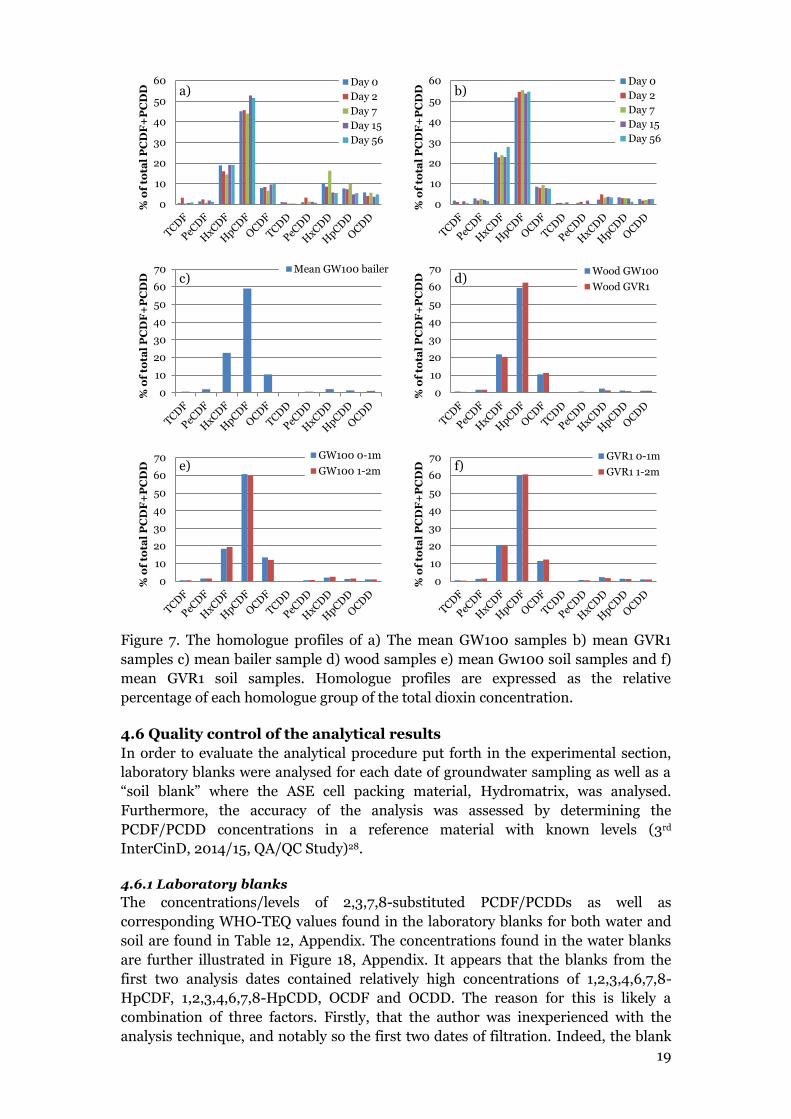
Figure 7 shows the homologue profiles of a) mean GW100 groundwater samples over
time b) mean GVR1 groundwater samples over time c) the mean GW100 bailer
sample d) the wood samples for the two sampling locations e) mean GW100 soil
samples and f) mean GVR1 soil samples. Overall, the profiles are highly similar and

18
we can be fairly certain that the source of the dioxins in groundwater is the
contaminated soil and wood found in the ground upgradient of the groundwater
wells. As for the GW100 groundwater the first three samples are notable as the
proportion of HxCDD and HpCDD are higher and the corresponding furans are
found in somewhat lower proportions, especially the sample from Day 7 which
corresponds to the peak shown in Figure 3. Indeed, the major trend for both
(pumped) groundwater types appear to be that HxCDDs, HpCDDs and OCDDs are
found in greater proportions than in the soil and wood samples, at the expense of the
corresponding PCDFs. One would expect, if different homologue profiles were
observed for soil and groundwater profiles, that PCDF/PCDDs with a higher aqueous
solubility as well as lower values of Kow and Kpw would be found to a higher extent in
the groundwater10–13. In this case the situation is the opposite. Whatever the means
for this dioxin mobilisation are, the most hydrophobic dioxins appear to have a
somewhat higher affinity than the furans for something in the groundwater. The
dioxin mobilisation will be further addressed in section 4.8.
The bailer, wood and soil samples have virtually the same homologue profile. This
further verifies that the original source of contamination is the same for both areas.
Although this was assumed at the start of the study, such verification is found
agreeable. The fact that the bailer has the same profile as soil is not surprising as the
majority of PCDF/PCDDs indeed came from soil particles present in the groundwater
sample.
In the pre-study by Fernerud Engineering, historical records were stated to show that
a pentachlorophenol based impregnating agent named “Dowicide” was used as the
main wood preservation agent at Norrbyskär2. Indeed, a pentachlorophenol based
impregnating agent termed “Dowicide G” has been widely used in Sweden4.
However, the homologue profiles of all the samples in this study do not correspond
to the PCDF/PCDD-profile found in Dowicide G. As shown by Persson et al.4,
Dowicide G is dominated by approximately 75% OCDD and 15% HpCDD (estimated
from Figure 3a in Persson et al.). The acquired homologue profiles at Norrbyskär are
much more similar (almost identical) to the PCDF/PCDD-profiles found in a
preservative termed Ky-5, which is a 2,3,4,6-tetrachlorophenol based preservative4,
Figure 6. Based on a PubChem Open Chemistry Database search an alternative name
for this preservative, distributed as a sodium salt, is “Dowicide F”38. Perhaps the
historical records only mentioned “Dowicide” and an assumption was made that this
stood for the commonly used preservative Dowicide G.
Figure 6. The chemical structure of the main active constituent, 2,3,4,6-
tetrachlorophenol, in the suspected original contamination source, the wood
preservative marketed as Ky-54 or Dowicide F38.
OCl
Cl
Cl
Cl
H
H
19
Figure 7. The homologue profiles of a) The mean GW100 samples b) mean GVR1
samples c) mean bailer sample d) wood samples e) mean Gw100 soil samples and f)
mean GVR1 soil samples. Homologue profiles are expressed as the relative
percentage of each homologue group of the total dioxin concentration.
4.6 Quality control of the analytical results
In order to evaluate the analytical procedure put forth in the experimental section,
laboratory blanks were analysed for each date of groundwater sampling as well as a
“soil blank” where the ASE cell packing material, Hydromatrix, was analysed.
Furthermore, the accuracy of the analysis was assessed by determining the
PCDF/PCDD concentrations in a reference material with known levels (3rd
InterCinD, 2014/15, QA/QC Study)28.
4.6.1 Laboratory blanks
The concentrations/levels of 2,3,7,8-substituted PCDF/PCDDs as well as
corresponding WHO-TEQ values found in the laboratory blanks for both water and
soil are found in Table 12, Appendix. The concentrations found in the water blanks
are further illustrated in Figure 18, Appendix. It appears that the blanks from the
first two analysis dates contained relatively high concentrations of 1,2,3,4,6,7,8-
HpCDF, 1,2,3,4,6,7,8-HpCDD, OCDF and OCDD. The reason for this is likely a
combination of three factors. Firstly, that the author was inexperienced with the
analysis technique, and notably so the first two dates of filtration. Indeed, the blank
0
10
20
30
40
50
60
% o
f to
tal
PC
DF
+P
CD
D Day 0
Day 2
Day 7
Day 15
Day 56
0
10
20
30
40
50
60
% o
f to
tal
PC
DF
+P
CD
D Day 0
Day 2
Day 7
Day 15
Day 56
0
10
20
30
40
50
60
70
% o
f to
tal
PC
DF
+P
CD
D Mean GW100 bailer
0
10
20
30
40
50
60
70
% o
f to
tal
PC
DF
+P
CD
D Wood GW100
Wood GVR1
0
10
20
30
40
50
60
70
% o
f to
tal
PC
DF
+P
CD
D GW100 0-1m
GW100 1-2m
0
10
20
30
40
50
60
70
% o
f to
tal
PC
DF
+P
CD
D GVR1 0-1m
GVR1 1-2m
a) b)
c) d)
e) f)

20
from 11-09-2015 was contaminated as the vacuum pump was shut off prior to
removing the tubing (and thus vacuum) to the suction flask. This caused back-flow of
water from the vacuum pump into to the sample. Furthermore it is suspected that the
metal grids used in the filtration apparatus (which were used over and over again)
had not been treated at 550° C prior to the first filtration (which was the routine
later), but only rinsed with acetone and toluene at these occasions. Additionally,
there might be some contaminations that arise from the ASE 350’s needle. This
hypothesis is based on the fact that levels of 1,2,3,7,8,9-HxCDF, 2,3,4,6,7,8-HxCDF,
1,2,3,4,7,8-HxCDD,1,2,3,4,6,7,8-HpCDF, 1,2,3,4,7,8,9-HpCDF, 1,2,3,4,6,7,8-HpCDD,
OCDF and OCDD were found in the soil blank as well, Figure 17, Appendix. The high
1,2,3,4,6,7,8-HpCDF as well as OCDF values may largely be due to cross-
contamination between the samples, but the rest of the PCDF/PCDDs are found in
(proportionally) higher amounts than in the actual samples. This suggests additional
contamination from an unknown source. Indeed the proportions of PCDF/PCDDs
found in the groundwater blanks and the soil blank were different from the
proportions found in the samples.
For further evaluation, Table 13 and 14, Appendix, show the proportion of each
concentration that the blank accounts for (i.e. blank/sample 100), for groundwater
and soil respectively. In these tables, samples where the blank levels correspond to
50% or more are marked with a red “*”. Levels of PCDF/PCDDs that were found
close to the limit of detection were naturally accounted for much more by the blank
levels than PCDF/PCDDs found in very high amounts. For the GW100 groundwater
samples two trends are observed: levels of 1,2,3,7,8,9-HxCDF, as well as the levels of
most congeners from Day 2 (excluding 1,2,3,4,6,7,8-HpCDF) are accounted for
largely, if not entirely, by the blank concentrations. As for the GVR1 groundwater
samples, the same trends are observed and additionally 1,2,3,4,6,7,8-HpCDD and
OCDD as well as all congeners in the samples from Day 0.
The highest levels of 1,2,3,7,8,9-HxCDF were only three times as high as the limit of
detection, and overestimated levels of this congener should not greatly increase the
WHO-TEQ (about 0.3 pg/kg groundwater). As for the samples acquired Day 2 it is
reasonable to assume that the concentrations and WHO-TEQ values are slightly
overestimated due to contamination during sample preparation. Levels of
1,2,3,4,6,7,8-HpCDD and OCDD in GVR1 were mostly accounted for by the blank
concentrations, with the exception of Day 7. This fact indicates that the relatively
high proportions of these congeners in the GVR1 groundwater homologue profile
(above) are exaggerated. As the WHO-TEFs for these congeners are very low21, the
WHO-TEQ should not be influenced to a great extent. That the GVR1 concentrations
were influenced by blank concentrations at Day 0 are to large extent due to the low
dioxin concentrations found that day. This means that the WHO-TEQ (Figure 13,
Appendix) and 2,3,7,8-dioxin concentrations found at Day 0 are exaggerated (Figure
4).
4.6.2 Determination of PCDF/PCDD concentrations in a reference material
In order to assess the accuracy of the analytical procedure, PCDF/PCDD-
concentrations of a given reference material (3rd InterCinD, 2014/15, QA/QC
Study)28, were determined and compared to consensus data by means of a Z-score
method39. Z-scores are the number of standard deviations from a consensus mean. A
criterion for good quality is that the determined values should be within 2 standard
deviations of the consensus mean value39. Table 3 shows the acquired Z-scores from

21
this study and the Z-scores from a previous analysis of the same reference material at
the Environmental Chemistry Laboratory, Umeå University.
Table 3. Quality control of the method used (starting at the extraction step): Z-score
method. Z = the number of standard deviations from mean consensus value.
Compound
(2,3,7,8-PCDF/PCDDs) Z-score My data
Z-score Env. Chem. data
2378-TCDF 0,62 0,12
2378-TCDD 1,6 -0,49 12378-PeCDF 0,53 0,85
23478-PeCDF 1,5 1,1
12378-PeCDD 2,0 0,26 123478-HxCDF 2,5a 0,25
123678-HxCDF -0,43 0,60 123789-HxCDF 1,2 1,6
234678-HxCDF 0,69 -0,28
123478-HxCDD 4,9a 1,5 123678-HxCDD -1,1 -0,26
123789-HxCDD 0,29 0,50 1234678-HpCDF -0,55 1,0
1234789-HpCDF -0,22 -0,25
1234678-HpCDD 0,81 1,2 OCDF 0,48 1,2
OCDD 0,65 1,0 a = outside 2 standard deviations
Overall, the obtained values are well within two standard deviations, with two
exceptions: 1,2,3,4,7,8-HxCDF and 123478-HxCDD. The reason for this deviation
from the consensus mean is likely the parameters used when performing the
integrations in Mass-Lynx. These congeners co-elute from the GC with 1,2,3,6,7,8-
HxCDF and 1,2,3,6,7,8-HxCDD respectively, which are values below the mean
consensus value. The parameters and mathematical functions for discrimination
between peaks can be set and adjusted in the software. In this case the criterion for
this discrimination was visual only, i.e. when the discrimination “looked good”.
Please note that the same settings were used in the software for the integration of all
PCDF/PCDDs and samples in this report. Perhaps greater care should have been
taken when adjusting these settings and someone with greater experience with Mass-
Lynx should have been consulted. Based on the rest of the Z-scores it is likely that all
data would be within two standard deviations if these steps had been taken. Even
though the amounts of 1,2,3,4,7,8-HxCDF and 123478-HxCDD may be
overestimated and 1,2,3,6,7,8-HxCDF and 1,2,3,6,7,8-HxCDD underestimated, the
discussion in section 4.6.1 is still valid as the same criterions were used for both
blanks and samples.
4.7 Additional analyses
For each (pumped) groundwater replicate, a 250 mL plastic bottle was filled and sent
to ALcontrol AB in Umeå for analysis of DOC and suspended particles. Data on
suspended particles was reported so low that it was deemed no point in looking at it
further (personal communication with Nadja Lundgren at Tyréns AB, Umeå). That
the data was so low seems strange as approximately only 100 mL groundwater
clogged a 0.45 µm polyamide filter Day 7. As for DOC, the results are plotted in
Figure 8, and 9 (GW100 and GVR1 respectively) together with corresponding WHO-

22
TEQ lower bound (LB) values. WHO-TEQ LB is the WHO-TEQ when all values under
detection limit are assumed to be 0.
Figure 8 shows GW100 DOC and WHO-TEQ LB levels over time. It seems that the
DOC and WHO-TEQ LB were not correlated to each other several days after the
excavation as the peak in DOC Day 2, corresponded to a “dip” in WHO-TEQ
concentrations. Furthermore, when the WHO-TEQ LB concentration was observed
as a peak Day 7, the DOC, in turn, “dipped”. It should be noted that the WHO-TEQ
followed the same trend as 2,3,7,8-PCDF/PCDD concentrations (Figure 3) as well as
the homologue concentrations (Figure 11, Appendix). Concentrations acquired in the
other, parallel, project22 mentioned in section 4.1.1 showed that the GW100
concentrations appeared to be correlated to DOC prior to the excavation Thus it
seems that the main mode of mobilisation changed for a short period after the
excavation, from DOC to something else. This is further discussed in section 4.8
Figure 8. GW100 dissolved organic carbon (DOC, mg/L water) and WHO-TEQ lower
bound (pg/kg water) over time (0, 2, 7, 15 and 56 days after excavation). Please note
that the DOC is plotted on the left y-axis and that WHO-TEQ is plotted on the right
y-axis.
As for GVR1, Figure 9, the situation appears to have been different. The DOC and the
WHO-TEQ LB followed the same trends, with an initial dip in concentration followed
by a small peak. If DOC is compared with the 2,3,7,8-PCDF/PCDDs it is observed
that 1,2,3,4,6,7,8-HpCDF did not have the same “dip” at Day 2 but otherwise
followed the same trend as DOC. OCDF and OCDD appeared to follow the DOC, but
the changes are harder to detect the lower the specific 2,3,7,8-PCDF/PCDD
concentration were. When looking at the homologue concentrations, Figure 12,
Appendix, the same trend was observed for the homologue group HpCDF as for
1,2,3,4,6,7,8-HpCDF. OCDF and HxCDF appeared to follow the DOC-trend. HxCDD
concentration peaked at Day 2, but the concentration was comparatively low. It
should be noted that Day 2 also coincided with significant clogging of filters,
signifying large amounts of suspended particles. In Figure 5, it was observed that a
part of 1,2,3,4,6,7,8-HpCDF was situated on particles, but to a minority. It could thus
be argued that the majority of 1,2,3,4,6,7,8-HpCDF followed DOC, but also that a
notable fraction were situated on particles. Effectively, this likely resulted in that the
“dip” of concentration of this congener was not seen in Figure 4. Indeed, as the
0
1
2
3
4
5
6
7
8
9
10
0
5
10
15
20
25
30
0 10 20 30 40 50 60
Σ W
HO
-TE
Q (
pg
/kg
wa
ter
)
DO
C (
mg
/ L
)
Days after excavation
DOC GW100 Σ WHO-TEQ (LB)

23
concentrations in GVR1 appear to have followed the DOC, it is suspected that DOC is
responsible for mobilisation in this system.
Figure 9. GVR1 dissolved organic carbon (DOC, mg/L water) and WHO-TEQ lower
bound (pg/kg water) over time (0, 2, 7, 15 and 56 days after excavation). Please note
that the DOC is plotted on the left y-axis and that WHO-TEQ is plotted on the right
y-axis.
4.8 Mobilisation of 2,3,7,8-PCDF/PCDDs
This section will be dedicated to discussing the above presented results with
reference to scientific literature. Shortly, the results presented in the previous
sections are: 1) the same dominant 2,3,7,8-PCDF/PCDDs were found throughout all
samples. 2) The excavation process had a marked effect on 2,3,7,8-PCDF/PCDD
concentrations found in GW100 but not GVR1 (based on the time points analysed).
3) It is suspected that GVR1 had a similar peak in concentration as GW100, but this
likely occurred in between the investigated time points. 4) The majority of dioxins
were adsorbed on particles >0.45 µm in GW100 groundwater and in the case of
GVR1 the dioxins appear to be present mainly in the dissolved phase. 5) In both
groundwater wells, the amount of dioxins in the dissolved phase increased over time
as the amount associated with particles decreased. 6) The particle rich bailer-samples
gave rise to approximately 100 times higher concentrations than the samples
acquired via low-flow pumping. 7) All analysed soils were contaminated, but the soil
from 1-2m depth was more so than the soil from 0-1 m depth. 8) The PCDF/PCDD-
concentration in the sampled wood pieces was generally lower than in the soil
samples. The 2,3,7,8-PCDF/PCDD-profiles appear to be approximately the same for
wood, bailer and soil samples which verifies that the contamination source most
likely is the same. 9) The homologue profiles were highly similar throughout all
groundwater, soil and wood samples and the source of the contamination was
suggested to be “Dowicide F”, i.e. a 2,3,4,6-tetrachlorophenol based wood
preservative. 10) The general trend for the (pumped) groundwater samples appeared
to be that HxCDDs, HpCDDs and OCDDs were found in higher proportions than in
the soil and wood samples, at the expense of the corresponding PCDFs (at least for
GW100). 11) GW100 2,3,7,8-PCDF/PCDD concentrations did not follow the DOC-
levels the days after the excavation, however in GVR1 they appeared to do so. The
quality control section is discussed independently above.
0
1
2
3
4
5
6
0
5
10
15
20
25
30
0 10 20 30 40 50 60
Σ W
HO
-TE
Q (
pg
/kg
wa
ter
)
DO
C (m
g /
L)
Days after excavation
DOC GVR1 Σ WHO-TEQ (LB)

24
Three aspects of the results jointly points to that the dioxins in the GW100
groundwater were mainly mobilized (as a result of excavation) on soil colloids,
namely: 1) what appeared to be clear groundwater clogged the 0.45 µm polyamide
filters during filtration, especially so the dates when the highest dioxin
concentrations were found, 2) the majority of 2,3,7,8-PCDF/PCDDs in the “split”
GW100 groundwater samples were found in the particulate phase (≥0.45 µm) and 3)
GW100 groundwater did not appear to follow DOC several days after the excavation.
The results in the present study suggest that the main dioxin mobilisation (as a result
of excavation) in GVR1 groundwater occurs via association with DOC, more
specifically: 1) significant clogging of polyamide filters was not associated with a
particularly large increase in PCDF/PCDD concentrations (except for a small
increase of 1,2,3,4,6,7,8-HpCDF), 2) the majority of 2,3,7,8-PCDF/PCDDs in the
“split” GVR1 groundwater samples were found in the dissolved phase and 3) GVR1
groundwater concentrations appeared to follow the DOC levels.
In order to understand the results, definitions of DOC and colloids must be made.
The International Union of Pure and Applied Chemistry (IUPAC) definition of
colloids is that they are particles that are not subject to gravitational forces due to
their small size and which have at least 1 dimension between 1 µm and 1 nm40.
Persson et al.41 defined the colloidal fraction as particles between 0,7 – 0.2 µm.
Vignati and Dominik40 divided colloids into “coarse colloids” (in the range between
1.2 – 0.45 µm) and small colloids (smaller than 0.45 µm). Furthermore, they defined
the fraction passing through a 0.45 µm filter as “small colloids and the truly
dissolved fraction”. The DOC analysis provided by ALcontrol followed the European
standard EN 1484, which defines DOC as carbon-containing compounds that pass
through a 0.45 µm (pose size) filter42. Indeed this appears to be a common definition
and readily found in scientific literature43–45. It should be noted, however, that some
authors consider DOC to be (dissolved) organic carbon that passes through a 0.22
µm filters as exemplified by the work done by Pokrovsky and Shirokova46.
Furthermore, it is important to remember that the membrane filtrate not only
contains DOC, but also other organic fractions such as dissolved organic
phosphorous and dissolved organic nitrogen. The entirety of the organic fraction is
thus classified as dissolved organic matter (DOM)43. Quoting Evans et al.43, [the
number of different compounds that may pass through a 0.45 µm filter] “is
effectively limitless, and it is thus impossible to provide a general chemical
description of DOM.” Hopefully, the above mentioned definitions of colloids and
DOC aid in illustrating that the actual dioxin transport is very complex, even when
only considering their affinity to colloidal particles or DOC. Colloidal particles may
be smaller than the common definition of DOC (0.45 µm), and DOC does not
indicate how the organic carbon is dissolved. Is DOC dissolved as “particles”, “truly
dissolved” or both? At what size does a “particle” stop being a particle and can be
regarded as “truly dissolved”? An entire paper could be dedicated to searching for
answers to the above posed questions. The present thesis will not deal with these
questions further, but the exact mechanism for dioxin mobilisation cannot be
elucidated without them.
Typically large, bulky and foremost highly lipophilic compounds such as
PCDF/PCDDs are considered immobile in soil due to their high sorption to organic
matter 31,41,47–49. Even so, PCDF/PCDDs have previously been observed to be mobile
in soil due to particle and DOC facilitated transport47. The PCDF/PCDDs found in

25
this study were mainly highly chlorinated and it has been found that such
compounds easily associate with colloid particles due to their large logKow41. Indeed,
the majority of dioxins found in a column leaching test were found to be associated
with natural colloids41. Persson et al.50 have previously found that the majority of
PCDDs in groundwater from an old Swedish sawmill site were associated with
colloidal particles (see Figure 1 in that study, the table includes a contaminated
sample which is excluded in the Figure). Additional findings were that PCDF was
most prevalent in larger particles (i.e. not colloids according to their definition) and
that PCDFs were more readily found in the dissolved phase than PCDDs which was
attributed to the generally higher water solubility of these compounds (relative to
degree of chlorination). In the present study, mainly PCDFs were obtained and were
for GW100 most likely associated with colloids, and for GVR1 associated with DOC,
which differ from their results. However, the fact that they observed a small fraction
of dissolved (<0.2 µm) PCDFs indicate that they indeed may be associated with DOC.
Their study also showed that PCDDs had a very high affinity for colloidal particles
which might help explain why higher relative levels of dioxins are found in the
groundwater samples (mainly GW100) than in the soil in the present study. Exactly
why the PCDD are enriched on the (suspected) colloids and/or DOC remains,
however, to be elucidated. It might require surface and component characterisation
of the soil, particles and DOC. Frankki et al.51 hypothesized that “POM possess in
average larger hydrophobic structures than DOM that in turn are more favourable
for the partitioning of the most hydrophobic contaminants” (POM being an
abbreviation for particulate organic matter). This explanation could help elucidate
why dioxins were likely found on colloids in GW100 groundwater. It is not applicable
to dioxins in GVR1 groundwater, unless they were associated particles smaller than
0.45 µm. The currently used definition of DOM does not allow for this, however. Kim
et al.52 concluded that (in a laboratory experiment) increased concentrations of
dissolved humic matter resulted in increased leachability of PCDF/PCDDs, which
seems consistent with the association of GVR1 PCDF/PCDDs with DOC.
Mobility of dioxins may also be facilitated by the presence of co-contaminants or
“facilitators” such as surfactants that are present at concentrations higher than their
critical micelle concentrations48. PCDF/PCDDs also partition to a greater extent in
organic solvents than in soil and as a consequence wood-preserving oil containing
pentachlorophenol can act as a carrier of dioxins31. In the case of the data acquired in
this study, little information exists of co-contaminants. Additionally it may be argued
that such mobile compounds are likely not present to-date, as the contamination
took place around a century ago.
Mechanisms for DOC-facilitated transport nature appear to be difficult to find in
scientific literature. The same can be said for soil colloids. Indeed, it is stated by
Grolimund et al.53 that: “The processes of particle generation and transport in
natural subsurface porous media are still poorly understood” and “particle transport
studies with colloidal particles and porous media are rather scarce”. However,
inorganic colloidal particles appear to have been well studied as may be exemplified
by the massive review by Ryan and Elimelech54. In the discussion above it was stated
that sizes of colloids and DOC may overlap and what DOC actually consists of is
poorly defined. Indeed, Persson et al.41 stated that: “Dissolved organic carbon or fine
particles may be transported through the soil profile as colloids”, so the actual mode
of transport for DOC may very well be via small colloidal particles. If both the soil
colloids and the DOC observed in the present study are regarded as solubilised

26
particles (of varying size), it is the author’s view that concepts from inorganic colloid-
facilitated transport may be applied to further understand the observed mobilisation
at Norrbyskär.
In order for colloid-facilitated transport to arise three main criteria are required: 1)
formation of mobile colloid particles, 2) association of contaminant (PCDF/PCDDs)
with said colloids and 3) the subsequent transport of such contaminant-associated
particles in groundwater. This has been stated for both inorganic and soil
colloids53,54. According to the review by Ryan and Elimelech54, two main processes
can account for “1) generation of mobile colloid particles”, namely chemical
perturbations in the groundwater and physical perturbations. Chemical
perturbations likely have little effect in the present study, as no chemicals were
introduced into the system. However, chemical equilibriums should have been
disturbed as a consequence of physical perturbations. This likely caused the observed
changes in DOC concentrations. Physical perturbations were further categorized into
perturbations during groundwater sampling, rapid infiltration of water through soils
and colloid mobilisation by groundwater flow through fractured soil54. In the present
study all of these situations may have had an effect on colloid generation and DOC (if
viewed as small colloids) release. Low flow pumping was utilized in order to avoid
perturbations in the groundwater wells23,24. Nevertheless, the pumping rate (between
100 and 200 mL per minute) was slightly higher than the recommended flow-rate for
avoidance of colloids i.e. 100 mL per minute25. This may have caused some artefacts
but they should likely be small as the flow-rate was not greatly exceeded. Rapid
infiltration of water likely contributed little to the mobilisation of colloids at
Norrbyskär, though some periods were particularly rainy. Together with the
fracturing of the soil, however, it might have played a role in the mobilisation. The
excavation process certainly fractured the soil and this unnatural perturbation
should have caused a significant formation of soil colloids which were mobilised by
the groundwater flow through this disrupted media. Furthermore, it likely had an
effect of DOC concentrations. As for the mobilisation of dioxins the experiment was
set up so that horizontal transport 5 m downstream could be detected, and so it was.
However, this study was not set up in such a way that the extent of the mobilisation
could be estimated, i.e. it is not known how far these mobilised particles and DOC
were transported before deposition.
The present study showed that the fraction of dioxins associated with the dissolved
phase appeared to increase over time. Based on the above discussion that DOC may
consist of smaller colloids, this process may be attributed to the phenomenon of size
exclusion. Size exclusion suggests that smaller particles have more “paths” to take
through the ground than the large particles. The large particles subsequently move
faster than the smaller particles through the pores of the media, in this case soil53,54.
The soil system may thus be regarded like an unrefined version of size exclusion
chromatography55.
As for factors influencing the mobility in a soil colloidal system, Grolimund et al.53
concluded that divalent cations such as Ca2+ and Mg2+ influence fate, stability and
reactivity of colloidal particles. A change in pH between 4.0 and 5.5 did not affect the
rate of deposition of such particles but changes of pore water velocity did. They also
concluded that such deposition follows first order kinetics53. Persson et al.41 saw that
the pore water velocity did not significantly affect the mobilisation of soil particles
and that such changes did not really influence parameters such as pH, dissolved

27
organic carbon, turbidity and concentrations of PCDF/PCDD. However, they also
concluded that their method was less suitable for highly hydrophobic compounds41,
such as the main contaminants in the present study. For DOC, Mertens el al.56
concluded that the spatial variability in fluxes of DOC in the deeper horizons of
investigated soil in the field was mainly related to water flux. Hydrophobic fractions
of DOM forms strong complexes with, and is flocculated by, Al3+ 51. Such interactions
may thus help form colloids which subsequently can mobilise highly organic
pollutants such as PCDF/PCDDs.
5. Conclusions
A significant effect of excavation on groundwater levels of 2,3,7,8-PCDF/PCDDs was
observed in this study. Concentrations of WHO-TEQs, homologue groups and
individual 2,3,7,8-PCDF/PCDD congeners notably increased in the groundwater well
GW100 a few days after the excavation. Furthermore, it was argued that the
groundwater in the other well (GVR1) likely behaved in a similar fashion, although in
between measured data points.
After the excavation, dioxins in the GW100 groundwater appeared to be mainly
mobilised by particles ≥0.45 µm and dioxins in GVR1 mainly associated with the
dissolved phase, and appeared to follow DOC levels.
The first week after the excavation appears critical and, in retrospect, more samples
should have been obtained during this period. However, this may not be true for
other similar systems as the mobility should depend on factors such as the soil,
ground water flow and distance from the excavation points to the downgradient
wells. As the excavated soil was put back after the excavation it is important to note
that the effect presented in this report may correspond to a worst case scenario.
An unexpected result was that the original contaminant was found to likely be
another impregnation agent than what has been stated in previous studies of the site.
Based on homologue profile analysis, the author suggested that the original
contamination source was the 2,3,4,6-tetrachlorophenol based preservative Dowicide
F which has a similar composition as the preservative Ky5.
As for uncertainties of the study, relatively high blank levels of highly chlorinated
dioxins were observed in the groundwater samples, especially the first two samples.
Largely, this is due to the low levels present in the groundwater samples. The soil
levels were not really influenced by blank levels due to their inherent high
concentrations of dioxins. Careful attention should perhaps be given in order to trace
these contaminations, which did not quite exhibit the same fingerprints as the
samples. The author suspects that contaminants were associated with metal grids
used in the beginning of this study as well as possible contaminants in the ASE and
possibly even the GC-HRMS system. Additionally, some cross-contamination in
between samples is likely to have occurred. Nevertheless, analysis of a reference
sample showed that the quantification was accurate, although the discrimination
between some co-eluting peaks was suboptimal. Fortunately, these peaks were not
found in significant levels in any of the samples in this study and due to the nature of
WHO-TEQs, these values remained unchanged, as did the levels of homologue
groups.

28
The author has not been able to identify any similar studies; where an upgradient soil
perturbation caused mobilisation of PCDF/PCDD contaminants via groundwater.
The novelty of these results may help in future understanding of similarly
contaminated soil-groundwater systems and suggest that additional thought should
be given prior to initiating an excavation process – perhaps colloid formation or DOC
release may arise?
6. Outlook
The results of this study should be sufficient to establish that an excavation at
Norrbyskär will cause mobilisation of PCDF/PCDDs, likely both via association with
colloids, and DOC. As a consequence there is a risk of PCDF/PCDD transport and
subsequent contamination of the surroundings should a large scale excavation
process be undertaken.
Previous studies at Norrbyskär have concluded that sediment levels of the
surrounding aquatic systems were not notably higher than those of the Baltic Sea in
general. Furthermore, dioxins were not found in raspberries and potatoes and
concentrations found in sheep and fish from the site were below European Union
threshold values. Concentrations of dioxins were, however, found in aquatic
molluscs1. The fact that PCDF/PCDDs may be transported via groundwater could
affect both biota and surrounding sediments, should an excavation process take
place.
As an alternative to excavation at Norrbyskär, the author suggests that the
contaminated areas should be covered by non-contaminated masses such as e.g. sand
and soil, as was suggested as one of the remediation alternatives in a main study by
Tyréns AB1. It is essential that such masses should not contain leachable organic
matter that could mobilise dioxins in the soil below. Much smaller amounts of money
would need to be spent in this case and investments in informing tourists and locals
about the pollution at the site, as well as monitoring biota and groundwater, could be
made instead.
The mobilisation process is also very interesting from a scientific standpoint. In
order to understand the mobilisation further, characterisation of the soil, colloid
particles and DOC should be made. A good starting point for such characterisation
could be methods presented by Grolimund et al.53, where transmission electron
microscopy, estimation of particle size, hydrodynamic diameter, mineralogical
composition by X-ray diffraction analysis and electrophoretic mobility by means of
microelectrophoresis were used to study soil colloids. Persson et al.50 also utilized X-
ray photoelectron spectroscopy to characterize colloidal particles as well as Frankki,
et al.51 who used this technique to compare organic carbon chemistry between both
DOM and POM.
For similar future studies the author would recommend that a groundwater well is
used as a negative control, i.e. no excavation is made upgradient of a specified
groundwater well. The sample replicates in this study were taken one after the other
and some variations may occur as a result of this sampling technique. More
representative replicates could likely be obtained by means of e.g. filling a third of
each of the replicate sampling bottles at the time, thus accounting for time dependent
differences during the sampling. If differences in colloidal particle sizes are of

29
interest, several filters with varying pore sizes could be used as done by Persson et al. 50. Furthermore, it would be very interesting if all samples were split according to
particulate and dissolved phases and subsequently characterised by techniques such
as those described above.
7. Acknowledgements
First and foremost, I would like to thank Staffan Lundstedt for being an incredible
supervisor. He’s been helping me every step of the way, from suggesting the project
in the first place to always taking time, even out of a busy schedule, to answer
questions and discuss the project. Thank you so much!
I would also like to thank Nadja Lundgren and Jeffrey Lewis at Tyréns AB for
allowing me to take part of the present project. Thank you both! Finally, I would like
to thank Per Liljelind for his help with the mass spectrometer and the related
software.

30
8. Appendix
8.1 Derivation of the formula used for quantification of dioxins
⁄
The ratio between the concentration of a native congener and one found in the 13C-labeled internal standard is the same as the ratio between the masses of these congeners.
The ratio between areas (chromatographic peak) of the native congener and the internal standard congener is the same as the ratio between the masses multiplied with a constant. This can also be thought of as a regression .
By rearranging the equation it can be solved for k. k is the same value in both the analysed sample and the quantification standard. As the mass of each congener in both the quantum standard (QS) and the internal standard is known, k can be solved from the quantification standard with added internal standard once areas from chromatographic peaks have been obtained.
(
)
Thus we define k as the above equation.
(
)
(
)
The relationship between sample (S) areas and masses can be written as the above equation.
Cn = Concentration of native congener (12C) mis = mass of congener in internal standard Cis = Concentration of internal standard congener (13C) Vn = Volume of native sample mn = mass of native congener Vis = Volume of internal standard
An = area of native congener Ais = area of internal standard congener k = constant

31
(
)
(
)
(
)
These two expressions can be combined as “k” is the same. The following equation is acquired:
(
)
(
)
(
)
As mis is the same for both expressions it is cancelled out and the following is acquired:
(
)
(
)
By rearranging this equation we get:
(
)
(
)
This equation can be used to calculate amounts of congeners in a sample based on known areas of the native congener and the internal standard congener in the sample and the quantification standard as well as the mass of congener in the quantification standard. In this study another version of this equation was used, namely:
(∑
∑ )
(∑
∑ )
The same result is acquired, but areas for both 35Cl and 37Cl are included. I.e. ∑An = An (12C and 35Cl) + An (12C and 37Cl) and ∑Ais = Ais (13C and 35Cl) + Ais (13C and 37Cl). This equation was used for each congener in each sample.

32
8.2 Additional Tables and Figures Table 4. Mean PCDF/PCDD concentrationsa of 2,3,7,8-PCDF/PCDDs and the sum of WHO-TEQ (higher and lower bound) in the groundwater samples. Compound
(2,3,7,8-PCDF/PCDDs)
GW100 mean groundwater PCDF/PCDD concentrations (pg/kg)
Sorted by days after excavation
GVR1 mean groundwater PCDF/PCDD concentrations (pg/kg)
Sorted by days after excavation
Day 0 Day 2 Day 7 Day 15 Day 56 Day 0 Day 2 Day 7 Day 15 Day 56
2378-TCDF <1.0 1.3 <1.0 <1.0 <1.0 <1.0 <1.0 <1.0 <1.0 <1.0
2378-TCDD <1.0 1.3 <1.0 <1.0 <1.0 <1.0 <1.0 <1.0 <1.0 <1.0
12378-PeCDF <1.0 1.4 <1.0 <1.0 <1.0 <1.0 <1.0 <1.0 <1.0 <1.0
23478-PeCDF 2.2 2.2 <1.0 <1.0 <1.0 3.5 <1.0 1.3 <1.0 <1.0
12378-PeCDD 2.0 1.2 1.6 <1.0 <1.0 <1.0 <1.0 <1.0 <1.0 <1.0
123478-HxCDF 3.2 3.2 5.2 <1.0 <1.0 3.3 2.2 2.9 <1.0 1.3
123678-HxCDF 3.1 2.1 3.3 <1.0 <1.0 1.6 <1.0 <1.0 <1.0 <1.0
123789-HxCDF 3.0 2.2 3.2 1.4 2.3 2.0 1.7 1.9 1.8 <1.0
234678-HxCDF 3.2 2.3 3.5 1.5 <1.0 2.5 2.6 2.1 1.6 1.3
123478-HxCDD <1.0 <1.0 <1.0 <1.0 <1.0 <1.0 <1.0 <1.0 <1.0 <1.0
123678-HxCDD 7.8 4.0 17 2.7 1.5 2.0 2.4 1.0 <1.0 <1.0
123789-HxCDD 3.5 1.8 8.7 <1.0 <1.0 <1.0 <1.0 <1.0 <1.0 <1.0
1234678-HpCDF 180 120 320 120 110 110 130 140 69 60
1234789-HpCDF 1.7 1.7 1.4 <1.0 <1.0 1.2 <1.0 <1.0 <1.0 <1.0
1234678-HpCDD 25 13 56 8.7 9.0 9.1 7.2 8.0 4.0 2.7
OCDF 47 36 75 33 33 34 31 40 18 15
OCDD 34 17 64 13 16 10 7.0 8.9 5.8 5.3
Σ WHO-TEQ (LB): 7.1 6.2 9.5 1.8 1.6 3.4 2.3 2.6 1.1 1.0
Σ WHO-TEQ (HB): 8.3 6.3 11 4.7 4.4 5.8 5.0 5.1 4.0 3.8 a: based on two replicates for each sample.

33
Figure 10. The WHO-TEQ values (pg/kg) for the mean GW100 groundwater samples over time.
Figure 11. Homologue group concentrations (pg/kg) for the mean GW100 groundwater samples. Error bars are given as the levels of the levels of the individual replicates.
Figure 12. Homologue group concentrations (pg/kg) for the mean GVR1 groundwater samples. Error bars are given as the levels of the levels of the individual replicates.
Figure 13. The WHO-TEQ values (pg/kg) for the mean GVR1 groundwater samples over time.
0
2
4
6
8
10
12
0 10 20 30 40 50 60
Σ W
HO
-TE
Q (
pg
/ k
g w
ate
r)
Days after excavation
Σ WHO-TEQ (LB)
Σ WHO-TEQ (HB)
0
100
200
300
400
500
600
0 10 20 30 40 50 60
Su
m o
f c
on
ge
ne
r c
on
ce
ntr
ati
on
(p
g /
kg
wa
ter
)
Days after excavation
Sum TCDF Sum TCDD
Sum PeCDF Sum PeCDD
Sum HxCDF Sum HxCDD
Sum HpCDF Sum HpCDD
OCDF OCDD
0
50
100
150
200
250
300
0 10 20 30 40 50 60
Su
m o
f c
on
ge
ne
r c
on
ce
ntr
ati
on
(p
g /
kg
wa
ter
)
Days after excavation
Sum TCDF: Sum TCDD:
Sum PeCDF: Sum PeCDD:
Sum HxCDF: Sum HxCDD:
Sum HpCDF: Sum HpCDD:
OCDF OCDD
0,0
1,0
2,0
3,0
4,0
5,0
6,0
7,0
0 10 20 30 40 50 60Σ
WH
O-T
EQ
(p
g /
kg
wa
ter
)
Days after excavation
Σ WHO-TEQ (LB):
Σ WHO-TEQ (HB):

34
Table 5. Mean concentrationsa of the sum of 2,3,7,8-PCDF/PCDDs in each homologue group and the total sum of PCDF, PCDD and PCDF+PCDD respectively for the groundwater samples.
Homologue group GW100 mean groundwater PCDF/PCDD concentrations (pg/kg)
Sorted by days after excavation
GVR1 mean groundwater PCDF/PCDD concentrations (pg/kg)
Sorted by days after excavation Day 0 Day 2 Day 7 Day 15 Day 56 Day 0 Day 2 Day 7 Day 15 Day 56
Sum TCDF 3.3 14 5.8 2.3 3.1 7.1 4.5 <1.0 3.6 1.2
Sum TCDD 6.6 4.0 3.9 1.3 1.1 2.4 3.0 1.6 2.3 <1.0
Sum PeCDF 8.5 11 9.2 6.4 4.0 11 7.3 11 5.0 3.2
Sum PeCDD 6.3 14 16 4.1 2.5 2.8 4.5 <1.0 4.2 <1.0
Sum HxCDF 110 69 170 66 62 99 89 100 54 55
Sum HxCDD 61 37 190 20 18 8.8 19 13 8.6 6.6
Sum HpCDF 270 200 500 180 170 200 210 240 130 110
Sum HpCDD 46 32 110 17 18 13 12 13 6.6 2.6
OCDF 47 36 75 33 33 34 31 40 18 15
OCDD 34 17 64 13 16 10 7.0 8.9 5.8 5.3
Total sum PCDF 440 330 760 290 270 360 350 390 210 180
Total sum PCDD 150 100 380 55 55 38 45 37 27 15
Total sum PCDF+PCDD 590 430 1100 350 330 400 400 430 240 200 a: based on two replicates for each sample.

35
Table 6. Congener concentrations of 2,3,7,8-PCDF/PCDDs and the sum of WHO-TEQ (higher and lower bound) in the split GW100-2 groundwater samples (filter or disc) and their corresponding full sample replicates, GW100-1.
Compound (2,3,7,8-PCDF/PCDDs)
GW100-1 groundwater PCDF/PCDD concentrations
(pg/kg) Sorted by days after excavation
GW100-2 groundwater PCDF/PCDD concentrations in discs, filters and the sum of discs and filters in “split” samples.
(pg/kg) Sorted by days after excavation and sample type
Day 7 Day 56 Day 7
Filter Day 7 Disc
Day 7 Sum
Day 56 Filter
Day 56 Disc
Day 56 Sum
2378-TCDF <1.0 <1.0 <1.0 <1.0 <1.0 <1.0 <1.0 <1.0 2378-TCDD <1.0 <1.0 <1.0 <1.0 <1.0 <1.0 <1.0 <1.0
12378-PeCDF 1.7 <1.0 <1.0 <1.0 <1.0 <1.0 <1.0 <1.0
23478-PeCDF 1.9 <1.0 <1.0 <1.0 <1.0 <1.0 <1.0 <1.0 12378-PeCDD 3.2 <1.0 <1.0 <1.0 <1.0 <1.0 <1.0 <1.0
123478-HxCDF 5.2 1.8 4.0 1.3 5.3 <1.0 <1.0 <1.0 123678-HxCDF 3.5 1.0 3.0 <1.0 3.0 <1.0 <1.0 <1.0
123789-HxCDF 2.6 1.7 2.1 1.7 3.8 1.3 1.7 3
234678-HxCDF 3.7 1.8 2.3 1.0 3.3 <1.0 <1.0 <1.0 123478-HxCDD <1.0 <1.0 <1.0 <1.0 <1.0 <1.0 <1.0 <1.0
123678-HxCDD 23 3.0 11 <1.0 11 <1.0 <1.0 <1.0 123789-HxCDD 12 1.1 5.9 <1.0 5.9 <1.0 <1.0 <1.0
1234678-HpCDF 300 120 290 52 340 68 37 105
1234789-HpCDF 2.8 <1.0 <1.0 <1.0 <1.0 <1.0 <1.0 <1.0 1234678-HpCDD 69 13 41 2.5 44 3.1 2.4 5.5
OCDF 72 39 67 12 79 16 10 26 OCDD 68 20 58 3.1 61 6.1 3.5 9.6
Σ WHO-TEQ (LB): 12 2.4 6.1 0.95 7.1 0.72 0.56 1.3
Σ WHO-TEQ (HB): 14 5.0 8.7 3.8 13 3.9 3.6 7.5

36
Table 7. Congener concentrations of 2,3,7,8-PCDF/PCDDs and the sum of WHO-TEQ (higher and lower bound) in the split GVR1-2 groundwater samples (filter or disc) and their corresponding full sample replicates, GVR-1.
Compound (2,3,7,8-PCDF/PCDDs)
GVR1-1 groundwater PCDF/PCDD concentrations
(pg/kg) Sorted by days after excavation
GVR1-1-2 groundwater PCDF/PCDD concentrations in discs, filters and the sum of discs and filters in “split” samples.
(pg/kg) Sorted by days after excavation and sample type
Day 7 Day 56 Day 7
Filter Day 7 Disc
Day 7 Sum
Day 56 Filter
Day 56 Disc
Day 56 Sum
2378-TCDF <1.0 <1.0 <1.0 <1.0 <1.0 <1.0 <1.0 <1.0 2378-TCDD <1.0 <1.0 <1.0 <1.0 <1.0 <1.0 <1.0 <1.0
12378-PeCDF <1.0 <1.0 <1.0 <1.0 <1.0 <1.0 <1.0 <1.0
23478-PeCDF 1.1 <1.0 <1.0 1.5 1.5 <1.0 <1.0 <1.0 12378-PeCDD <1.0 <1.0 <1.0 <1.0 <1.0 <1.0 <1.0 <1.0
123478-HxCDF 3.5 1.6 <1.0 2.2 2.2 <1.0 1.1 1.1 123678-HxCDF 1.4 <1.0 <1.0 <1.0 <1.0 <1.0 <1.0 <1.0
123789-HxCDF 1.5 <1.0 <1.0 2.2 2.2 <1.0 1.0 1.0
234678-HxCDF 2.3 1.5 <1.0 1.9 1.9 <1.0 1.1 1.1 123478-HxCDD <1.0 <1.0 <1.0 <1.0 <1.0 <1.0 1.1 1.1
123678-HxCDD 2.0 1.1 <1.0 <1.0 <1.0 <1.0 <1.0 <1.0 123789-HxCDD <1.0 <1.0 <1.0 <1.0 <1.0 <1.0 <1.0 <1.0
1234678-HpCDF 130 64 48 100 150 8.3 48 56
1234789-HpCDF <1.0 1.2 <1.0 <1.0 <1.0 <1.0 <1.0 <1.0 1234678-HpCDD 8.8 3.6 2.7 4.4 7.1 <1.0 1.7 1.7
OCDF 46 16 14 20 34 2.9 12 15 OCDD 9.1 7.7 3.7 5.1 8.8 1.6 1.2 2.8
Σ WHO-TEQ (LB): 2.8 1.1 0.51 2.1 2.6 0.08 0.93 1.01
Σ WHO-TEQ (HB): 5.1 3.9 3.7 4.7 8.4 3.2 3.7 6.9

37
Table 8. Mean congener concentrationsa of 2,3,7,8-PCDF/PCDDs and the sum of WHO-TEQ (higher and lower bound) in the bailer sample.
Compound (2,3,7,8-
PCDF/PCDDs)
GW100 mean bailer sample PCDF/PCDD concentration
(pg/kg)
2378-TCDF 7.3
2378-TCDD 4.7
12378-PeCDF 17
23478-PeCDF 51
12378-PeCDD 24
123478-HxCDF 180
123678-HxCDF 150
123789-HxCDF 43
234678-HxCDF 110
123478-HxCDD 5.7
123678-HxCDD 56
123789-HxCDD 26
1234678-HpCDF 11000
1234789-HpCDF 82
1234678-HpCDD 220
OCDF 3000
OCDD 310
Σ WHO-TEQ (LB): 220
Σ WHO-TEQ (HB): 220 a: based on two bailer replicates.
Table 9. Mean concentrationsa of the sum of 2,3,7,8-PCDF/PCDDs in each homologue group and the total sum of PCDF, PCDD and PCDF+PCDD respectively in the bailer sample.
Homologue group GW100 mean bailer sample PCDF/PCDD concentration
(pg/kg)
Sum TCDF 180
Sum TCDD 42
Sum PeCDF 580
Sum PeCDD 190
Sum HxCDF 6600
Sum HxCDD 630
Sum HpCDF 17000
Sum HpCDD 400
OCDF 3000
OCDD 310
Total sum PCDF 28000
Total sum PCDD 1600
Total sum PCDF+PCDD 30000 a: based on two bailer replicates.
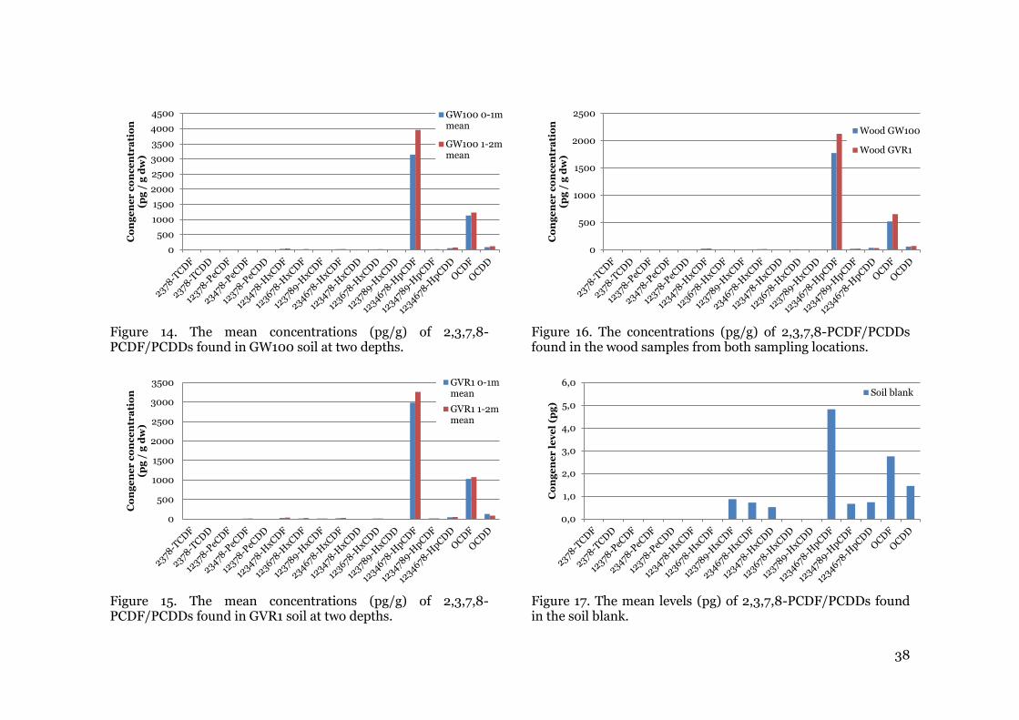
38
Figure 14. The mean concentrations (pg/g) of 2,3,7,8-PCDF/PCDDs found in GW100 soil at two depths.
Figure 15. The mean concentrations (pg/g) of 2,3,7,8-PCDF/PCDDs found in GVR1 soil at two depths.
Figure 16. The concentrations (pg/g) of 2,3,7,8-PCDF/PCDDs found in the wood samples from both sampling locations.
Figure 17. The mean levels (pg) of 2,3,7,8-PCDF/PCDDs found in the soil blank.
0
500
1000
1500
2000
2500
3000
3500
4000
4500
Co
ng
en
er
co
nc
en
tra
tio
n
(pg
/ g
dw
)
GW100 0-1mmean
GW100 1-2mmean
0
500
1000
1500
2000
2500
3000
3500
Co
ng
en
er
co
nc
en
tra
tio
n
(pg
/ g
dw
)
GVR1 0-1mmean
GVR1 1-2mmean
0
500
1000
1500
2000
2500
Co
ng
en
er
co
nc
en
tra
tio
n
(pg
/ g
dw
)
Wood GW100
Wood GVR1
0,0
1,0
2,0
3,0
4,0
5,0
6,0
Co
ng
en
er
le
ve
l (p
g)
Soil blank

39
Table 10. Mean congener concentrationsa of 2,3,7,8-PCDF/PCDDs and the sum of WHO-TEQ (higher and lower bound) in soil samples as well as concentrations found in wood samples.
Compound (2,3,7,8-
PCDF/PCDDs)
GW100 mean soil PCDF/PCDD concentrations
(pg/g dw) Sorted by sample depth
GVR1 mean soil PCDF/PCDD concentrations
(pg/g dw) Sorted by sample depth
GW100 wood PCDF/PCDD
concentrations (pg/g dw)
GVR1 wood PCDF/PCDD
concentrations (pg/g dw)
0-1 m 1-2 m 0-1 m 1-2 m
2378-TCDF 2.5 3.4 1.5 2.7 2.3 1.7
2378-TCDD 0.59 2.8 <0.50 <0.50 0.77 <0.50
12378-PeCDF 3.6 5.1 3.3 3.9 2.4 3.3
23478-PeCDF 8.7 14 7.4 9.7 7.6 7.1
12378-PeCDD 6.1 9.4 2.2 3.1 4.4 2.7
123478-HxCDF 33 46 28 35 23 26
123678-HxCDF 15 28 12 21 12 11
123789-HxCDF 11 15 10 10 5.6 6.3
234678-HxCDF 26 31 20 27 14 16
123478-HxCDD <0.50 1.3 <0.50 <0.50 1.9 <0.50
123678-HxCDD 18 23 10 10 9.9 8.5
123789-HxCDD 10 10 4.9 4.7 5.2 3.8
1234678-HpCDF 3200 4000 3000 3300 1800 2100
1234789-HpCDF 16 23 13 15 21 23
1234678-HpCDD 58 83 45 49 36 34
OCDF 1100 1200 1000 1100 520 650
OCDD 90 120 130 84 62 71
Σ WHO-TEQ (LB): 53 73 44 51 30 33
Σ WHO-TEQ (HB): 53 73 44 51 30 33 a: based on two replicates for each soil sample. Only one replicate was used for each of the wood samples.

40
Table 11. Mean concentrationsa of the sum of 2,3,7,8-PCDF/PCDDs in each homologue group and the total sum of PCDF, PCDD and PCDF+PCDD respectively in soil and wood samples.
Homologue group GW100 mean soil PCDF/PCDD concentration
(pg/g dw) Sorted by sample depth
GVR1 mean soil PCDF/PCDD concentration
(pg/g dw) Sorted by sample depth
GW100 wood PCDF/PCDD concentration
(pg/g dw)
GVR1 wood PCDF/PCDD concentration
(pg/g dw)
0-1 m 1-2 m 0-1 m 1-2 m
Sum TCDF 44 63 24 45 40 35
Sum TCDD 14 26 7.1 11 12 4.3
Sum PeCDF 130 150 120 150 88 100
Sum PeCDD 46 84 27 28 38 13
Sum HxCDF 1500 2200 1400 1500 1100 1200
Sum HxCDD 170 250 96 85 120 81
Sum HpCDF 5100 6400 4700 5200 3000 3600
Sum HpCDD 110 160 76 81 65 52
OCDF 1100 1200 1000 1100 520 650
OCDD 90 120 130 84 62 71
Total sum PCDF 7900 10000 7300 8000 4700 5600
Total sum PCDD 430 640 330 290 300 220
Total sum PCDF+PCDD 8300 11000 7600 8300 5000 5800 a: based on two replicates for each soil sample. Only one replicate was used for each of the wood samples.

41
Table 12. Congener concentrations of 2,3,7,8-PCDF/PCDDs and the sum of WHO-TEQ (higher and lower bound) in the laboratory blanks for both groundwater and the “soil”.
Compound (2,3,7,8-
PCDF/PCDDs)
PCDF/PCDD concentrations/levels found in laboratory blanks (pg/kg – water, pg – soil)
Sorted by date (dd-mm-yy) and sample type (disc, filter, sum or full samples)
09-09-15
Full sample 11-09-15
Full sample 16-09-15
Full sample 24-09-15
Full sample 04-11-15
Filter 04-11-15
Disc 04-11-15
Sum Soil blank
(pg)
2378-TCDF <1.0 1.6 <1.0 <1.0 <1.0 <1.0 <1.0 <0.50 2378-TCDD <1.0 1.1 <1.0 <1.0 <1.0 <1.0 <1.0 <0.50
12378-PeCDF <1.0 1.8 <1.0 <1.0 <1.0 <1.0 <1.0 <0.50
23478-PeCDF <1.0 1.8 <1.0 <1.0 <1.0 <1.0 <1.0 <0.50 12378-PeCDD <1.0 1.7 <1.0 <1.0 <1.0 <1.0 <1.0 <0.50
123478-HxCDF 1.0 2.6 <1.0 <1.0 <1.0 <1.0 <1.0 <0.50 123678-HxCDF <1.0 1.9 <1.0 <1.0 <1.0 <1.0 <1.0 <0.50
123789-HxCDF 1.5 2.6 <1.0 1.6 <1.0 1.2 1.2 0.87
234678-HxCDF 1.4 1.7 <1.0 <1.0 <1.0 <1.0 <1.0 0.72 123478-HxCDD <1.0 <1.0 <1.0 <1.0 <1.0 <1.0 <1.0 0.52
123678-HxCDD 1.8 1.8 <1.0 <1.0 <1.0 <1.0 <1.0 <0.50 123789-HxCDD <1.0 1.9 <1.0 <1.0 <1.0 <1.0 <1.0 <0.50
1234678-HpCDF 12 9.2 3.8 3.5 1.2 3.8 5.0 4.83
1234789-HpCDF <1.0 1.9 <1.0 <1.0 <1.0 <1.0 <1.0 0.67 1234678-HpCDD 7.0 5.8 1.8 <1.0 1.0 1.5 2.5 0.74
OCDF 7.3 17 2.5 2.8 1.0 3.1 4.1 2.75 OCDD 15 15 2.9 3.1 1.4 3.9 5.3 1.45
Σ WHO-TEQ (LB): 0.77 5.0 0.060 0.19 0.02 0.17 0.19 0.27
Σ WHO-TEQ (HB): 3.5 5.1 3.2 3.2 3.2 3.2 6.4 1.69

42
Table 13. Proportion of the water blank 2,3,7,8-congener concentrations “in” groundwater samples (Blank/sample 100, %). When the sample concentration is under detection limit that value is given a 0.00. Compound
(2,3,7,8-PCDF/PCDDs)
Proportion of the blank “in” GW100 samples (Blank/sample 100, %)
Sorted by days after excavation
Proportion of the blank “in” GVR1 samples (Blank/sample 100, %)
Sorted by days after excavation
Day 0 Day 2 Day 7 Day 15 Day 56 Day 0 Day 2 Day 7 Day 15 Day 56
2378-TCDF 0.00 120* 0.00 0.00 0.00 0.00 0.00 0.00 0.00 0.00
2378-TCDD 0.00 86* 0.00 0.00 0.00 0.00 0.00 0.00 0.00 0.00
12378-PeCDF 0.00 130* 0.00 0.00 0.00 0.00 0.00 0.00 0.00 0.00
23478-PeCDF 0.00 81* 0.00 0.00 0.00 0.00 0.00 0.00 0.00 0.00
12378-PeCDD 0.00 150* 0.00 0.00 0.00 0.00 0.00 0.00 0.00 0.00
123478-HxCDF 32 81* 0.00 0.00 0.00 31 120* 0.00 0.00 0.00
123678-HxCDF 0.00 94* 0.00 0.00 0.00 0.00 260* 0.00 0.00 0.00
123789-HxCDF 50* 120* 0.00 110* 51* 75* 150* 0.00 86* 0.00
234678-HxCDF 45 75* 0.00 0.00 0.00 57* 65* 0.00 0.00 0.00
123478-HxCDD 0.00 0.00 0.00 0.00 0.00 0.00 0.00 0.00 0.00 0.00
123678-HxCDD 23 45 0.00 0.00 0.00 89* 74* 0.00 0.00 0.00
123789-HxCDD 0.00 104* 0.00 0.00 0.00 0.00 0.00 0.00 0.00 0.00
1234678-HpCDF 6.9 7.9 1.2 3.0 4.3 11 7.1 2.7 5.0 8.2
1234789-HpCDF 0.00 110* 0.00 0.00 0.00 0.00 0.00 0.00 0.00 0.00
1234678-HpCDD 28 45 3.2 0.00 28 77* 79* 23 0.00 94*
OCDF 16 48 3.3 8.4 12 22 55* 6.2 15 27
OCDD 43 86* 4.5 25 34 150* 210* 33 54* 100* * Blank concentrations make up more than 50% of the congener.

43
Table 14. Proportion of the soil blank 2,3,7,8-congener concentrations “in” soil samples (Blank/sample 100, %). When the sample concentration is under detection limit, that value is given as 0.
Compound (2,3,7,8-PCDF/PCDDs)
Proportion of the blank “in” soil samples (Blank/sample 100, %)
Sorted by sample
GW100 0-1m mean GW100 1-2m mean GVR1 0-1m mean GVR1 1-2m mean
2378-TCDF 0.00 0.00 0.00 0.00
2378-TCDD 0.00 0.00 0.00 0.00
12378-PeCDF 0.00 0.00 0.00 0.00
23478-PeCDF 0.00 0.00 0.00 0.00
12378-PeCDD 0.00 0.00 0.00 0.00
123478-HxCDF 0.00 0.00 0.00 0
123678-HxCDF 0.00 0.00 0.00 0
123789-HxCDF 34 38 37 47
234678-HxCDF 27 29 81* 28
123478-HxCDD 0.00 0.00 0.00 0.00
123678-HxCDD 0.00 0.00 0.00 0.00
123789-HxCDD 0.00 0.00 0.00 0.00
1234678-HpCDF 3.3 2.2 4.2 4.0
1234789-HpCDF 39 58* 0.00 120*
1234678-HpCDD 3.9 2.3 8.2 9.0
OCDF 6.7 5.1 8.4 8.5
OCDD 5.6 3.8 9.3 17 * Blank concentrations make up more than 50% of the congener.

44
Figure 18. The concentrations of 2,3,7,8-PCDF/PCDDs found in the laboratory groundwater blanks. The blanks are named after their filtration date.
0
2
4
6
8
10
12
14
16
18
20
Co
ng
en
er
co
nc
en
tra
tio
n
(pg
/ k
g w
ate
r)
150909150911150916150924151104 filter+disc

45
9. References
(1) Tyréns AB. Utvärderingsrapport - Huvudstudie Norrbyskär 2013
http://www.umea.se/download/18.3f589399144bbe9c36610600/1397631105
506/Utv%C3%A4rderingsrapport+Huvudstudie+Norrbysk%C3%A4r+2014-
04-09.pdf (accessed Apr 29, 2016).
(2) Fernerud Engineering. Miljöteknisk Förstudie Norrbyskär med avseende på
Sågverket 2010
http://www.umea.se/download/18.4166f9b6137178df873a29/1361887742413
/F%C3%B6rstudie_100326.pdf (accessed Apr 24, 2016).
(3) Levin, J.-O.; Rappe, C.; Nilsson, C.-A. Scand. J. Work. Environ. Health 1976,
2 (2), 71.
(4) Persson, Y.; Lundstedt, S.; Öberg, L.; Tysklind, M. Chemosphere 2007, 66 (2),
234.
(5) Fytianos, K.; Voudrias, E.; Kokkalis, E. Chemosphere 2000, 40 (1), 3.
(6) Kulkarni, P. S.; Crespo, J. G.; Afonso, C. A. M. Environ. Int. 2008, 34 (1), 139.
(7) Dopico, M.; Gómez, A. J. Air Waste Manag. Assoc. 2015, 65 (9), 1033.
(8) Ogura, I.; Masunaga, S.; Nakanishi, J. Chemosphere 2001, 45 (2), 173.
(9) Aries, E.; Anderson, D. R.; Fisher, R.; Fray, T. A. T.; Hemfrey, D. Chemosphere
2006, 65 (9), 1470.
(10) Yang, G.; Zhang, X.; Wang, Z.; Liu, H.; Ju, X. J. Mol. Struct. THEOCHEM
2006, 766 (1), 25.
(11) Shiu, W. Y.; Doucette, W.; Gobas, F. A. P. C.; Andren, A.; Mackay, D. Environ.
Sci. Technol. 1988, 22 (6), 651.
(12) Åberg, A.; MacLeod, M.; Wiberg, K. J. Phys. Chem. Ref. Data 2008, 37 (4),
1997.
(13) Govers, H. A. J.; Krop, H. B. Chemosphere 1998, 37 (9–12), 2139.
(14) Jones, K. C.; de Voogt, P. Environ. Pollut. 1999, 100 (1–3), 209.
(15) Sinkkonen, S.; Paasivirta, J. Chemosphere 2000, 40 (9–11), 943.
(16) Van den Berg, M.; Birnbaum, L.; Bosveld, A. T.; Brunström, B.; Cook, P.;
Feeley, M.; Giesy, J. P.; Hanberg, A.; Hasegawa, R.; Kennedy, S. W.; Kubiak,
T.; Larsen, J. C.; van Leeuwen, F. X.; Liem, A. K.; Nolt, C.; Peterson, R. E.;
Poellinger, L.; Safe, S.; Schrenk, D.; Tillitt, D.; Tysklind, M.; Younes, M.;
Waern, F.; Zacharewski, T. Environ. Health Perspect. 1998, 106 (12), 775.
(17) Abel, J.; Haarmann-Stemmann, T. Biol. Chem. 2010, 391 (11), 1235.
(18) White, S. S.; Birnbaum, L. S. J. Environ. Sci. Health Part C 2009, 27 (4), 197.
(19) Denison, M. S.; Soshilov, A. A.; He, G.; DeGroot, D. E.; Zhao, B. Toxicol. Sci.
2011, 124 (1), 1.
(20) van Leeuwen, F. X. R.; Feeley, M.; Schrenk, D.; Larsen, J. C.; Farland, W.;
Younes, M. Chemosphere 2000, 40 (9–11), 1095.
(21) Berg, M. V. den; Birnbaum, L. S.; Denison, M.; Vito, M. D.; Farland, W.;
Feeley, M.; Fiedler, H.; Hakansson, H.; Hanberg, A.; Haws, L.; Rose, M.; Safe,
S.; Schrenk, D.; Tohyama, C.; Tritscher, A.; Tuomisto, J.; Tysklind, M.;
Walker, N.; Peterson, R. E. Toxicol. Sci. 2006, 93 (2), 223.
(22) Utveklingsprojekt - Norrbyskär 2015
http://www.umea.se/download/18.3f589399144bbe9c36610609/1397631202
727/Bilaga+3+-+Utvecklingsprojekt+Norrbysk%C3%A4r.pdf (accessed Apr
29, 2016).
(23) Puls, R. W.; Powell, R. M. Ground Water Monit. Remediat. 1992, 12 (3), 167.
(24) Barcelona, M. J.; Wehrraann, H. A.; Varljen, M. D. Ground Water 1994, 32
(1), 12.

46
(25) Kearl, P. M.; Korte, N. E.; Cronk, T. A. Ground Water Monit. Remediat. 1992,
12 (2), 155.
(26) Liljelind, P.; Söderström, G.; Hedman, B.; Karlsson, S.; Lundin, L.; Marklund,
S. Environ. Sci. Technol. 2003, 37 (16), 3680.
(27) Dionex Application Note 323
http://www.dionex.com/en-us/webdocs/4329-AN323-ASE-Dibenzo-p-
Dioxins-Furans-21Jun2011-LPN0812-04.pdf (accessed May 2, 2016).
(28) Libralato, S. Accredia, 3rd InterCinD, 2014/15, QA/QC Study 2015
(29) Svenska Geotekniska Föreningen. Fälthandbok, Undersökningar av
förorenade områden 2013
http://www.commonforum.eu/Documents/Questionnaires/AEIRS/Falthandb
ok_Publicerad_2014.pdf (accessed Apr 22, 2016).
(30) Hoogsteen, M. J. J.; Lantinga, E. A.; Bakker, E. J.; Groot, J. C. J.; Tittonell, P.
A. Eur. J. Soil Sci. 2015, 66 (2), 320.
(31) Bulle, C.; Bertrand, F.; Samson, R.; Deschênes, L. Chemosphere 2008, 73 (1,
Supplement), 149.
(32) Laine, M. M.; Ahtiainen, J.; Wågman, N.; Öberg, L. G.; Jørgensen, K. S.
Environ. Sci. Technol. 1997, 31 (11), 3244.
(33) Nie, Z.; Die, Q.; Yang, Y.; Tang, Z.; Wang, Q.; Huang, Q. Environ. Sci. Pollut.
Res. 2014, 21 (13), 7863.
(34) Xu, M.; Yan, J.; Lu, S.; Li, X.; Chen, T.; Ni, M.; Dai, H.; Wang, F.; Cen, K.
Environ. Sci. Technol. 2009, 43 (4), 1023.
(35) Wu, W. Z.; Schramm, K.-W.; Xu, Y.; Kettrup, A. Water Res. 2001, 35 (12),
3025.
(36) Green, N. J. L.; Jones, J. L.; Jones, K. C. Environ. Sci. Technol. 2001, 35 (14),
2882.
(37) Zhang, H.; Ni, Y.; Chen, J.; Su, F.; Lu, X.; Zhao, L.; Zhang, Q.; Zhang, X.
Chemosphere 2008, 73 (10), 1640.
(38) Pubchem. Dowicide F | C6H2Cl4NaO+ - PubChem
https://pubchem.ncbi.nlm.nih.gov/compound/24180825#section=Top
(accessed Apr 24, 2016).
(39) Beckman Coulter. Quality control (QC) - Information and Troubleshooting
Guide
https://www.beckmancoulter.com/ucm/idc/groups/public/documents/webas
set/glb_bci_152294.pdf (accessed Apr 25, 2016).
(40) Vignati, D.; Dominik, J. Aquat. Sci. 2003, 65 (2), 129.
(41) Persson, Y.; Hemström, K.; Öberg, L.; Tysklind, M.; Enell, A. Chemosphere
2008, 71 (6), 1035.
(42) European standard EN1484
http://www.globallab.com.br/download/artigos/toc/norma_din_en_1484.pd
f (accessed May 20, 2016).
(43) Evans, C. D.; Monteith, D. T.; Cooper, D. M. Environ. Pollut. 2005, 137 (1),
55.
(44) Leenheer, J. A.; Croué, J.-P. Environ. Sci. Technol. 2003, 37 (1), 18A.
(45) Urban-Rich, J. J. Exp. Mar. Biol. Ecol. 1999, 232 (1), 107.
(46) Pokrovsky, O. S.; Shirokova, L. S. Water Res. 2013, 47 (2), 922.
(47) Weber, R.; Gaus, C.; Tysklind, M.; Johnston, P.; Forter, M.; Hollert, H.;
Heinisch, E.; Holoubek, I.; Lloyd-Smith, M.; Masunaga, S.; Moccarelli, P.;
Santillo, D.; Seike, N.; Symons, R.; Torres, J. P. M.; Verta, M.; Varbelow, G.;
Vijgen, J.; Watson, A.; Costner, P.; Woelz, J.; Wycisk, P.; Zennegg, M.
Environ. Sci. Pollut. Res. 2008, 15 (5), 363.

47
(48) Grant, S.; Mortimer, M.; Stevenson, G.; Malcolm, D.; Gaus, C. Environ. Sci.
Technol. 2011, 45 (2), 406.
(49) Bulle, C. S. M.; Samson, R.; Deschênes, L. Chemosphere 2011, 83 (2), 117.
(50) Persson, Y.; Shchukarev, A.; Oberg, L.; Tysklind, M. Environ. Sci. Pollut. Res.
2008, 15 (6), 463.
(51) Frankki, S.; Persson, Y.; Shchukarev, A.; Tysklind, M.; Skyllberg, U. Environ.
Pollut. 2007, 148 (1), 182.
(52) Kim, Y.-J.; Lee, D.-H.; Osako, M. Chemosphere 2002, 47 (6), 599.
(53) Grolimund, D.; Elimelech, M.; Borkovec, M.; Barmettler, K.; Kretzschmar, R.;
Sticher, H. Environ. Sci. Technol. 1998, 32 (22), 3562.
(54) Ryan, J. N.; Elimelech, M. Colloids Surf. Physicochem. Eng. Asp. 1996, 107, 1.
(55) Berek, D. J. Sep. Sci. 2010, 33 (3), 315.
(56) Mertens, J.; Vanderborght, J.; Kasteel, R.; Pütz, T.; Merckx, R.; Feyen, J.;
Smolders, E. J. Environ. Qual. 2007, 36 (2), 597.