mobile robot sonar for target localization and...

Mobile Robot Sonar for Target Localization andClassification1

LINDSAY KLEEMAN2 and ROMAN KUC3

AbstractA novel sonar array is presented that has applications in mobile robotics forlocalization and mapping of indoor environments. The ultrasonic sensor localizes andclassifies multiple targets in two dimensions to ranges of up to 8 meters. Byaccounting for effects of temperature and humidity, the system is accurate to within amillimeter and 0.1 degrees in still air. Targets separated by 10 mm in range can bediscriminated. The error covariance matrix for these measurements is derived toallow fusion with other sensors. Targets are statistically classified into four reflectortypes: planes, corners, edges and unknown.

The paper establishes that two transmitters and two receivers are necessaryand sufficient to distinguish planes, corners and edges. A sensor array is presentedwith this minimum number of transmitters and receivers. A novel design approach isthat the receivers are closely spaced so as to minimize the correspondence problem ofassociating different receiver echoes from multiple targets.

A linear filter model for pulse transmission, reception, air absorption anddispersion is used to generate a set of templates for the echo as a function of range andbearing angle. The optimal echo arrival time is estimated from the maximum cross-correlation of the echo with the templates. The use of templates also allowsoverlapping echoes and disturbances to be rejected. Noise characteristics are modeledfor use in the maximum likelihood estimates of target range and bearing.Experimental results are presented to verify assumptions and characterize the sensor.

1Work performed while L. Kleeman was on sabbatical leave at the Intelligent Sensors Laboratory,Department of Electrical Engineering, Yale University.2 Author for correspondence, Intelligent Robotics Research Centre, Department of Electrical andComputer Systems Engineering, Monash University, Wellington Rd, Clayton 3168, AUSTRALIA.3Intelligent Sensors Laboratory, Department of Electrical Engineering, Yale University, PO Box208284, New Haven CT 06520-8284, USA.

2

1. IntroductionUltrasonic sensors provide a cheap and reliable means for robot localization

and environmental sensing when the physical principles and limitations of theiroperation are well understood. This paper presents models and approaches that allowsensors composed of multiple transmitters and receivers to be exploited in asystematic, robust and accurate manner. A sensor design is presented that approachesthe fundamental physical limitations of sonar in terms of accuracy and discrimination.The performance is limited only by the physical properties of air, the reflectors andnoise.

The objective of our research is to investigate the optimal deployment ofultrasonic transducers and the associated signal processing for indoor roboticsapplications. We concentrate on environments composed of specular surfaces, suchas smooth walls, bookcases, desks and chairs, that reflect acoustic energy analogous toa mirror reflecting light. Rough surfaces can be treated with other techniques (Bozmaand Kuc 1991). The applications of primary interest are robot localization fromsensing known environmental features, such as wall and corner positions (Leonardand Durrant-Whyte 1991, Nagashima and Yuta 1992, Manyika and Durrant-Whyte1993), and conversely, mapping of unknown environments for later use forlocalization and navigation (Bozma and Kuc 1991a, Iijima and Yuta 1992, Bozma andKuc 1991, Elfes 1987, Crowley 1985, Moravec and Elfes 1985). Obstacle avoidance(Kuc 1990, Borenstein and Koren 1988) is another application of the sensor.

A classification standard for indoor target types emerging is that of planes,corners and edges (Bozma and Kuc 1991a, Barshan and Kuc 1990, Peremans et al1993, Sabatini 1992, Leonard and Durrant-Whyte 1991, McKerrow 1993). Thesensor approach presented here is novel in the sense that it classifies all three targettypes with the one stationary sensor, simultaneously in some cases, with high accuracyand discrimination. Our approach has higher speed and accuracy, particularly inbearing, compared to single transducer systems that rely on multiple displacedreadings and wheel odometery for target classification (Bozma and Kuc 1991,McKerrow 1993, Leonard and Durrant-Whyte 1991). Sonar sensors have beenreported previously that can classify two of the three target types -- Barshan and Kuc(1990) discriminate planes and corners based on pulse amplitude measurements; andPeremans et al (1993) uses time of flight (TOF) to classify planes and edges andemploys sensor movement to distinguish corners and planes. Three dimensional sonartarget classification based on pulse amplitude measurements is proposed in (Hong andKleeman 1992), where statistical tests are derived for classifying planes and concavecorners of two and three intersecting orthogonal planes. Other sonar array sensors thatreport range and bearing to targets have been reported (Munro et al 1989, Yang et al1992, Suoranta 1992, Manyika and Durrant-Whyte 1993) and proposed (Sabatini1992).

This paper is organized as follows: Section 2 establishes that a minimum oftwo transmitters and two receivers are required to classify planes, corners and edgeswithout sensor movement. The physical separation of the receivers is considered inSection 3 in relation to the important problem of establishing correspondence betweenmultiple echoes on two receivers. A solution is proposed that does not requireadditional transducers over the minimum for classification of planes, corners andedges. In Section 4 we consider the design of a sensor module called a vector sensorthat can measure both range and bearing to an ultrasonic target. In Section 5, the

3

vector sensor module is included as a component of a minimal transducer arrangementfor classifying planes, corners and edges. The interaction of the sensor to the threetarget types is derived and used to establish a statistical test for classifying targets. InSection 6 pulse shape is modeled as a function of range, transmitter and receiverangles, and air characteristics. These results allow the optimal estimation of distanceof flight (DOF) as described in Section 7 where error models are developed based onexperiments. Strategies for handling overlapping echoes and noise disturbances arediscussed in Section 8 and experimental results are presented in Section 9 to verify theperformance of the sensor. Conclusions and future extensions are given in the finalsection of the paper.

Throughout the paper, the terms transducer, transmitter and receiver refer toindividual ultrasonic devices, while sensor refers to a combination of transducers andintelligence required to actively sense the environment.

2. Minimum Sensor RequirementsIn this section, the minimum requirements of an array of transducers are

established in order to identify commonly occurring primitive reflector types in anindoor environment. The reflector types agreed upon in the literature (Barshan andKuc 1990, Peremans et al 1993, Sabatini 1992, Leonard and Durrant-Whyte 1991,McKerrow 1993) and considered in this paper are planes, corners and edges. A planereflector is assumed to be smooth and reflect ultrasound specularly. The corner isassumed to be a concave right angle intersection of two planes. An edge representsphysical objects such as convex corners and high curvature surfaces, where the pointof reflection is approximately independent of the transmitter and receiver positions.These reflector types are considered in two dimensions in this paper. For a mobilerobot, vertical planes, corners and edges are of interest. Since the robot is assumed tomove in a horizontal plane, the vertical coordinates of environmental features do notprovide essential information for localization and map building for localization. Thework presented here can be extended to three dimensional targets, if required, byincluding a second sensor that is rotated by 90o.

Although transmitters and receivers are considered separately, they may becombined into one physical transducer. We use the construct of virtual imagesborrowed from an optical context. The virtual image of a transducer in a plane isobtained by reflecting the true position of the transducer about the plane. The virtualimage of a transducer in a corner is obtained by reflecting about one plane and thenthe other which results in a reflection about the line of intersection of the planes.

First, we establish that one transmitter and any number of receivers areinsufficient to distinguish corners from planes in any orientation. Any receiver in atransducer array will see the virtual image of the transmitter sensor reflected in theplane or corner. The sensing problem is entirely equivalent to replacing the reflectorand transmitter by a transmitter placed at the position of the virtual image transmitter.No matter how many receivers are present, the corner and plane are indistinguishablein terms of distance of flight when only one transmitter is employed, as illustrated inFigure 1(a). Note however that the virtual image orientation of the transmitter isreversed between the plane and the corner. With this orientation of plane, it isconceivable to distinguish planes from corners using the amplitude of the receivedpulse, since the amplitude is a function of the absolute value of angles of transmissionand reception (Barshan and Kuc 1990). However, the two virtual images are identical

4

in orientation when the plane is aligned with the transmitter as shown in Figure 1(b).Therefore in general, planes and corners are not distinguishable with just onetransmitter.

T

Plane

Corner

Virtual image

T'

T T'

R

R

R arbitarily positioned

(a)

T

Plane

Corner

Virtual image

T'

T T'

R

R

R arbitarily positioned

(b)

Figure 1 Indistinguishability of planes and corners using DOF. (a) Plane notaligned with Transmitter (T) - virtual images observed at Receiver (R) are

indistinguishable with DOF but distinguishable with amplitude of echo pulse.(b) Plane aligned with Transmitter - virtual images indistinguishable between

plane and corner.

Can any number of transmitters and one receiver distinguish planes fromcorners? The construction in Figure 2 shows the virtual image, Rplane, of a receiverin an arbitrarily positioned plane. If the vertex of a corner is positioned at theintersection between the line joining the receiver to its image and the plane, then thereceiver sees the same DOF for both transmitters. Moreover, for planes aligned withthe receiver, the virtual images in the plane and corner coincide exactly in orientation.This case renders the corner and the plane indistinguishable, even with pulseamplitude measurements. Therefore, for the general case of any orientation, at leasttwo transmitters and two receivers are required for differentiation of planes andcorners.

R

T1

Tn

Virtual image of receivers

RplaneRcorner

. . .

Figure 2 - Virtual images of a receiver in a plane and corner for n transmitters.

5

As will be seen below, the configuration of two transmitters and two receiversis sufficient to discriminate planes, corners and edges, and hence the important resultfollows:

Two transmitters and two receivers are necessary and sufficient fordiscriminating planes, corners and edges in two dimensions.

Designs of sensors have been published (Peremans et al 1993, Sabatini 1992)with one transmitter and three receivers, that can discriminate planes from edges andcorners from edges, but require movement of the sensor to discriminate planes fromcorners. The sensor movement is equivalent to placing another transmitter at the newlocation. The use of three receivers provides redundancy that can be exploited in anattempt to solve the correspondence problem, described in the next section.

3. The Correspondence Problem and Receiver SeparationIn an ideal environment containing only one reflector, each echo is directly

attributed to the reflector. In practice many reflectors are present and multiple echoesare observed on each receiver channel. The correspondence problem is how toassociate echoes on different receivers with each other and ultimately to physicalreflectors. The more general association problem of mapping multiple observations tomultiple physical sources occurs in many areas of robotics and computer vision.

When an incorrect association is made between incoming echoes on differentreceivers, gross errors can occur. For example a reflector's bearing can be incorrectlyreported by a large margin, producing phantom targets unrelated to physical objects.The effect on robot navigation and mapping depends on the robustness of higher levelinterpretation of sensor readings.

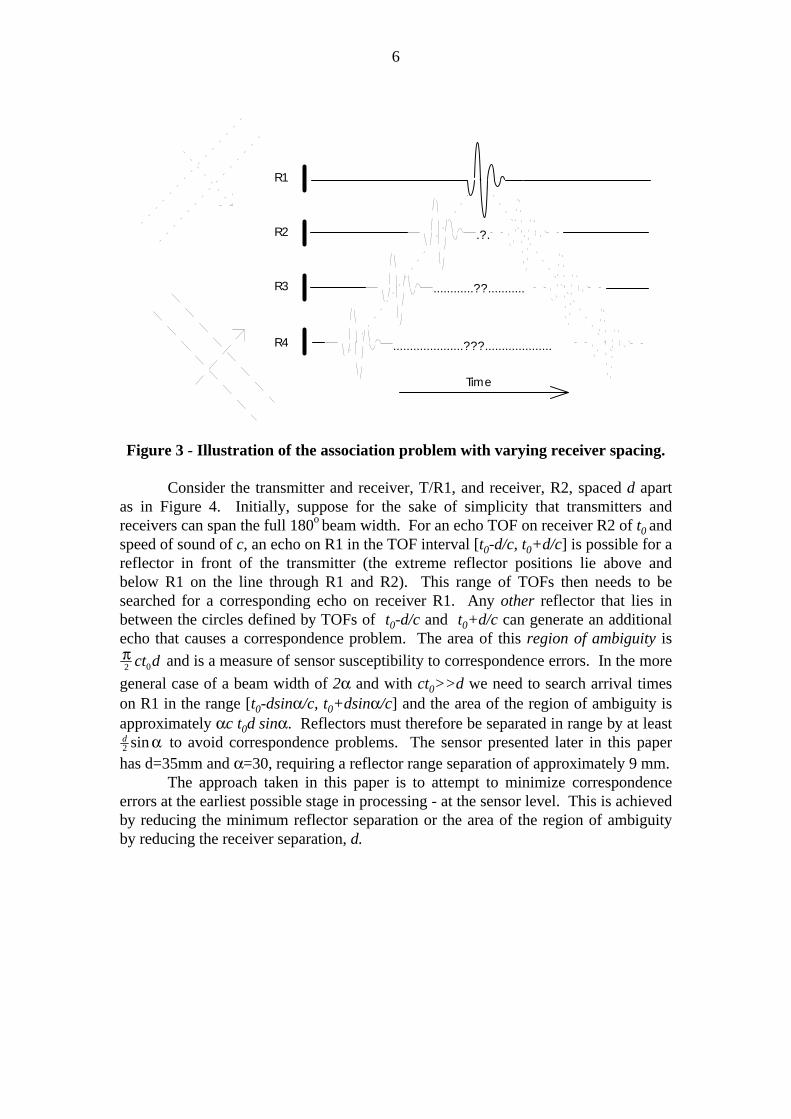
Four equally spaced receivers R1, R2, R3 and R4 are shown in Figure 3. Anecho is received on R1 and we wish to find the corresponding echoes on R2, R3 andR4 for the same wave front. For a given angular beam width of the receivers, theextremes of arrival directions are represented by the dashed and dotted wave fronts inFigure 3. These arrival directions define the search time intervals on receiverchannels R2, R3 and R4 about the arrival time of the echo on R1. The ends of thesearch time intervals are shown with dotted and dashed pulse outlines. Note that thesearch interval spreads in proportion to the separation between R1 and the otherreceiver, and thus increasing the chance of incorrect associations. For widely-spacedreceivers, occlusion problems can result in the absence of an echo on the otherreceiver and no association is then possible.

6

.?.

............??...........

.....................???....................

Time

R1

R2

R3

R4

Figure 3 - Illustration of the association problem with varying receiver spacing.

Consider the transmitter and receiver, T/R1, and receiver, R2, spaced d apartas in Figure 4. Initially, suppose for the sake of simplicity that transmitters andreceivers can span the full 180o beam width. For an echo TOF on receiver R2 of t0 andspeed of sound of c, an echo on R1 in the TOF interval [t0-d/c, t0+d/c] is possible for areflector in front of the transmitter (the extreme reflector positions lie above andbelow R1 on the line through R1 and R2). This range of TOFs then needs to besearched for a corresponding echo on receiver R1. Any other reflector that lies inbetween the circles defined by TOFs of t0-d/c and t0+d/c can generate an additionalecho that causes a correspondence problem. The area of this region of ambiguity isπ2 0ct d and is a measure of sensor susceptibility to correspondence errors. In the more

general case of a beam width of 2α and with ct0>>d we need to search arrival timeson R1 in the range [t0-dsinα/c, t0+dsinα/c] and the area of the region of ambiguity isapproximately αc t0d sinα. Reflectors must therefore be separated in range by at leastd2 sin α to avoid correspondence problems. The sensor presented later in this paperhas d=35mm and α=30, requiring a reflector range separation of approximately 9 mm.

The approach taken in this paper is to attempt to minimize correspondenceerrors at the earliest possible stage in processing - at the sensor level. This is achievedby reducing the minimum reflector separation or the area of the region of ambiguityby reducing the receiver separation, d.

7

R2

d

region of correspondence

T/R1

d

x1

x2

x1+x2=t0/c

possible reflector positions

Figure 4 - Region of ambiguity - reflectors in this region cause a correspondenceproblem.

A possible disadvantage of small receiver separation is that less accuratebearing information may be extracted from arrival times in the presence of noise.With the sensor design described later in the paper, high accuracy in bearing angle hasbeen achieved despite the receivers being spaced as close as the transducers physicallyallow.

Due to our closely-spaced receivers, correspondence problems are rare and arehandled by simply discarding the measurements that have a correspondenceambiguity. Other approaches are to use information such as echo power and shape toresolve ambiguity. Redundant receivers can be employed also, such as in threereceiver systems (Peremans et al 1993). However, the presence of noise in thereceived signals or certain geometric arrangements may still cause unreliablecorrespondences.

4. Vector SensorIn this section we show how two receivers can be combined to form a vector

sensor which measures bearing to a target in addition to the range available from onereceiver. The vector sensor will be used later as a useful building block in a sensor.Just one transducer and the echo pulse amplitude can be employed to extract theabsolute value of the angle of arrival as described in (Barshan and Kuc 1990, Hongand Kleeman 1992, Sabatini 1992). However, we require the sign of the arrival anglefor a complete sensor system. Moreover, the use of amplitude measurements as ameans of bearing estimation is avoided in this paper due the requirement to detectedges and cylinders whose reflected echo amplitude depends on the geometricproperties of the target, such as surface curvature.

In a two dimensional plane, the angle of reception of an echo can be foundfrom the arrival times of two receivers. For plane wave fronts as shown in Figure 5,the angle to the normal of the receivers, θ, is given by

8

θ = sin-1 c t

ddiff�

��

(1)

where tdiff is the difference in arrival times, c is speed of sound and d is the receiverseparation.

d

θd sin θ

R1

R2

plane wave

Figure 5 - Plane wave arrival at two receivers.

In practice, a plane wave front is an approximation for a spherical wave frontemerging from a point source. The point source may be attributed to a reflector withhigh curvature such as an edge or cylinder and consequently acts as a point source atthe range of the reflector. Alternatively, the point source can arise due to the virtualimage of a transmitter reflected in a plane or corner and acts as a point source withtwice the range as the reflector. Both these cases are modeled as the point source P inFigure 6, where r1 and r2 are the distances from P to the receivers R1 and R2. Forplanes and corners r1 and r2 are directly available from the DOFs from the transmitterto receivers. In the case of an edge reflector, r1 is half the DOF for a transmitter atthe same position4 as R1 and r1-r2 is the difference in DOFs.

θ

R1

R2

P

A

B

r2

r190−θd

Figure 6 - Point source geometry for two receivers.

4 With an edge reflector and a transmitter at different position to R1, r1 and r2 can be still expressed asfunction of DOFs and the transmitter position.

9

From the cosine rule on triangle APB:

r d r d r22 2

12

12 90= + − −cos( )θ (2)

and hence

θ = + −��

��

−sin 12

12

22

12d r r

d r (3)

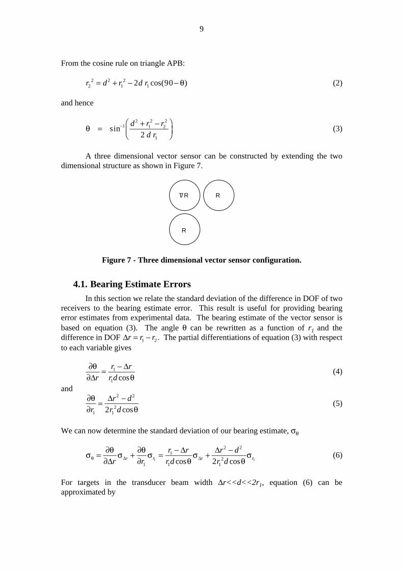
A three dimensional vector sensor can be constructed by extending the twodimensional structure as shown in Figure 7.

T/R R

R

Figure 7 - Three dimensional vector sensor configuration.

4.1. Bearing Estimate Errors

In this section we relate the standard deviation of the difference in DOF of tworeceivers to the bearing estimate error. This result is useful for providing bearingerror estimates from experimental data. The bearing estimate of the vector sensor isbased on equation (3). The angle θ can be rewritten as a function of r1 and thedifference in DOF ∆r r r= −1 2 . The partial differentiations of equation (3) with respectto each variable gives

∂θ∂ θ∆

∆r

r rrd

= −1

1 cos (4)

and∂θ∂ θr

r dr d1

2 2

122

= −∆cos

(5)

We can now determine the standard deviation of our bearing estimate, σθ

σ ∂θ∂

σ ∂θ∂

σθ

σθ

σθ = + = − + −∆

∆ ∆∆ ∆r r

r rrd

r dr dr r r r

1

1

1

2 2

121 12cos cos

(6)

For targets in the transducer beam width ∆r<<d<<2r1, equation (6) can beapproximated by

10

σθ

σθ

σθ ≈ −12 1

2 1dd

rr rcos cos∆ (7)

The second term in equation (7) is much smaller than the first and can beignored in practice. For small bearing angles we have the approximation

σ σθ ≈ ∆r

d (8)

5. Application of Vector Sensor to Plane/Corner/EdgeIdentification

The sensor arrangement employed in experiments reported in this paper isshown in Figure 8. There are two receivers and two transmitters which is theminimum required to identify planes, corners and edges. The two receivers areclosely spaced to minimize any correspondence ambiguity and also to form a vectorsensor as described in the previous section. The transmitters are spaced sufficiently toperform reflector classification at the furthest range conceived for the sensor of 5 to 7meters. The transducers are Polaroid 7000 series devices (Polaroid 1987).

The sensor arrangement has one less receiver than other published systems(Peremans et al 1993, Sabatini 1992). This is a significant saving due to the datacapture and processing requirements of a receiver channel. The deployment of asecond transmitter in the sensor is comparatively cheap in terms of hardware, but doesincur an additional measurement delay since transmitters need to be fired alternately.The sensor is stationary for results reported this paper. At the expense of sensoraccuracy, onboard robot odometry measurements can compensate for a movingsensor. A future smart sensor may be able to exploit the absence of reflectors atcertain ranges to overlap transmission.

T/R R T

35mm 225mm

T/V

Figure 8 - Sensor arrangement, T=transmitter R=receiver V=vector receiver.

The sensor arrangement is interfaced to a 33 MHz 386 PC via a Biomation8100 dual channel transient recorder with 8 bit conversion at a sample rate of 1 MHzas shown in Figure 9. The PC controls the firing of the transmitters and the triggeringand control of the Biomation transient recorder. All processing and display of thereceived data are performed on the PC. The interface electronics consists of twosimple receiver preamplifiers and two single transistor transmitter circuits. A 300VDC power supply provides the transducer biasing.

11

PC 386

InterfaceElectronics

BiomationDual channel8 BIT ADC 1MHz

Trigger R2 dataR1 data

Trigger and fire controlT2

R2

R1/T1

Digital data

Control

Figure 9 - Experimental Setup for Sensor.

The interaction of the sensor with each of the reflector types is derived in theSections 5.1, 5.2 and 5.3. Statistical tests for classification into plane, corner, edge orunknown reflector type are derived from these geometrical relationships in Section5.4.

5.1. Plane Geometry

Figure 10 shows the sensor encountering a plane reflector. Note that the tworeceivers and transmitter labeled as T/V act as a transmitter and vector receiver at thelocation of the transmitter when bearing is estimated using equation (3). This ispossible due to the assumption of a plane reflector allowing the distance to be knownto the point source that is the virtual image in this case.

T2 T2'

T1/V T1/V'

b b

α1α2

β

VIRTUAL IMAGE

α1

b sin α1

b cos α1r2

r1

A

Figure 10 - Sensor image in plane reflector.

From the geometry in Figure 10, the range, r2, and bearing, α2, of the virtualimage T2' are functions of the range, r1, and bearing, α1, of the virtual image T1'.Consequently, we can write r2plane(r1, α1) and α2plane(r1, α1). From triangle T1/VT2' A, the bearing difference between the two transmitters is

12

β ααplane

b

r b=

−��

��

−tancos

sin1 1

1 1

(9)

andα α α β2 1 1 1plane planer( , ) = + (10)

r r r b b

r r b bplane2 1 1 1 1

21

2

12

1 122

( , ) ( sin ) ( cos )

sin

α α αα

= − += − +

(11)

Note that the plane must be sufficiently wide to produce the two reflections. Forr1>>b, the plane must be at least (b cosα1)/2 wide.

5.2. Corner Geometry

The virtual image of the sensor in a corner is obtained by reflecting the sensorabout one plane of the corner and then the other plane. This gives rise to a reflectionthrough the point of intersection of the corner as shown in Figure 11. The situation issimilar to the plane except that the angle between the transmitter images, β, isopposite in sign:

β ααcorner

b

r b= −

−��

��

−tancos

sin1 1

1 1

(12)

α α α β2 1 1 1corner cornerr( , ) = + (13)

r r r r b bcorner2 1 1 12

1 122( , ) sinα α= − + (14)

To be seen fully by the sensor, the corner must subtend an arc of approximatelytan-1(2b/r1).

T2

T2'

T1/V

T1/V'

b

b

α1α2 −β

VIRTUAL IMAGE

α1

b sin α1

b cos α1

r2

r1 A

Figure 11 - Sensor image in corner reflector.

13

5.3. Edge Geometry

An edge represents physical objects such as convex corners and high curvaturesurfaces, where the point of reflection is approximately independent of transmitter andreceiver positions. Consequently, the reflection from an edge has equal bearings fromeach transmitter (α2edge(r1, α1) =α1). The DOF r2edge is obtained from the cosinerule:

r r r r r

r r b r b

edge2 1 1 1 2 1

1 12 2

1 1

2 2

4 4

2

( , ) / ( / )

sin

α

α

= + −

=+ + −

(15)

T2

T1/V

b

α1 = α2

r2 - r1/2

r1/2edge reflector

Figure 12 - Sensor with an edge reflector.

5.4. Geometric Hypothesis Testing

In this section we determine statistical tests for discriminating between planes,corners and edges. We assume that our reflectors are geometrically perfect in thesense that planes are perfectly flat and edges act as a point reflector. Imperfections inreflectors will be discussed in conjunction with experimental data in Section 9.

From the previous three sections, the differences between planes, corners andedges can be seen in terms of the sensor perception. To discriminate planes, cornersand edges, the angle difference between bearings of the two transmitters can be used,since it is β for a plane, -β for a corner and 0 for an edge. The DOF information canbe exploited to aid differentiation of edges from corners and planes. For example inFigure 13 the bearing and DOF are shown for the three reflector types at a range of

0.5 meters. For small bearing angles and range much larger than b, β ≈ b

r1. Also for

the DOF r2 the difference between a corner or plane and an edge is approximately b

r

2

12.

As ranges increase these margins decrease while standard deviations of errors inbearing and DOF increase, and a range limit for the sensor discrimination capability isreached at the range where the margins and errors are equal.

14

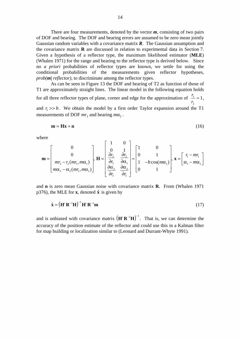
There are four measurements, denoted by the vector m, consisting of two pairsof DOF and bearing. The DOF and bearing errors are assumed to be zero mean jointlyGaussian random variables with a covariance matrix R. The Gaussian assumption andthe covariance matrix R are discussed in relation to experimental data in Section 7.Given a hypothesis of a reflector type, the maximum likelihood estimator (MLE)(Whalen 1971) for the range and bearing to the reflector type is derived below. Sinceno a priori probabilities of reflector types are known, we settle for using theconditional probabilities of the measurements given reflector hypotheses,prob(m| reflector), to discriminate among the reflector types.

As can be seen in Figure 13 the DOF and bearing of T2 as function of those ofT1 are approximately straight lines. The linear model in the following equation holds

for all three reflector types of plane, corner and edge for the approximation of r

r1

2

1≈ ,

and r b1 >> . We obtain the model by a first order Taylor expansion around the T1measurements of DOF mr1 and bearing mα1 .

m Hx n= + (16)

where

m H x=−−

�

�

�

��

=

�

�

�

��

≈−

�

�

�

��

=−−

��

��

0

0

1 0

0 1 1 0

0 1

1

0 12 2 1 1

2 2 1 1

2

1

2

1

2

1

2

1

1

1 1

1 1mr r mr m

m mr m

r

r

r

r r

b m

r mr

m( , )

( , )

,cos( )

,α

α α α

∂∂

∂∂α

∂α∂

∂α∂

α α α

and n is zero mean Gaussian noise with covariance matrix R. From (Whalen 1971p376), the MLE for x, denoted $x is given by

$ ' 'x H R H H R m= − − −1 1 1 � (17)

and is unbiased with covariance matrix H R H' − −1 1 � . That is, we can determine the

accuracy of the position estimate of the reflector and could use this in a Kalman filterfor map building or localization similar to (Leonard and Durrant-Whyte 1991).

15

alpha1 (degrees ) ->

-40

-30

-20

-10

0

10

20

30

40

plane

edge

corner

alpha1 (degrees ) ->

900

950

1000

1050

1100

1150plane/corner edge

Figure 13 - Received angle and DOF for transmitter 2 for r1=1 meter.

We can evaluate the confidence associated with each target type hypothesis byexamining the noise residual of our MLE for each reflector. The weighted sum ofsquare errors, S

S = − −−( $ )' ( $ )Hx m R Hx m1 (18)

has a chi-square distribution with four degrees of freedom (Papoulis 1984). A 95%confidence corresponds to S≤ 0 71. and 80% to S≤ 1 65. . If none or more than onereflector type has an acceptable confidence level then the target is classified asunknown. This situation arises when the errors in the bearing and range are too largeto effectively discriminate reflector types. The sensor will then report lack ofdiscrimination - an important feature.

It is also possible (but unlikely) that a range/bearing measurement may match,to an acceptable confidence level, more than one other range/bearing measurementsderived from the other transmitter. We adopt the "fail safe" approach and classify allthe ambiguous range/bearing measurements as unknown. This approach effectivelyavoids the correspondence problem of associating range/bearing measurements ondifferent transmitters. More sophisticated approaches are left for future research.

6. Modeling Pulse ShapeEstimating bearing and range to reflectors depends on an accurate TOF

estimate. The maximum likelihood estimate of TOF of an echo pulse with additiveGaussian white noise is obtained by finding the maximum of the correlation functionof the received pulse with the known pulse shape (Woodward 1964). Knowing thepulse shape in the absence of noise is important for determining TOF and also foridentifying overlapping echoes and disturbances as discussed in Section 8. Modelingpulse shape is therefore considered important for robustness and performance of thesensor design. Note that the pulse amplitude is also modeled in this section but is notemployed in the arrival time determination.

16

Reflector

s(t)

rec(t)

hair

hreflhtrans

hrec

θT

θ R

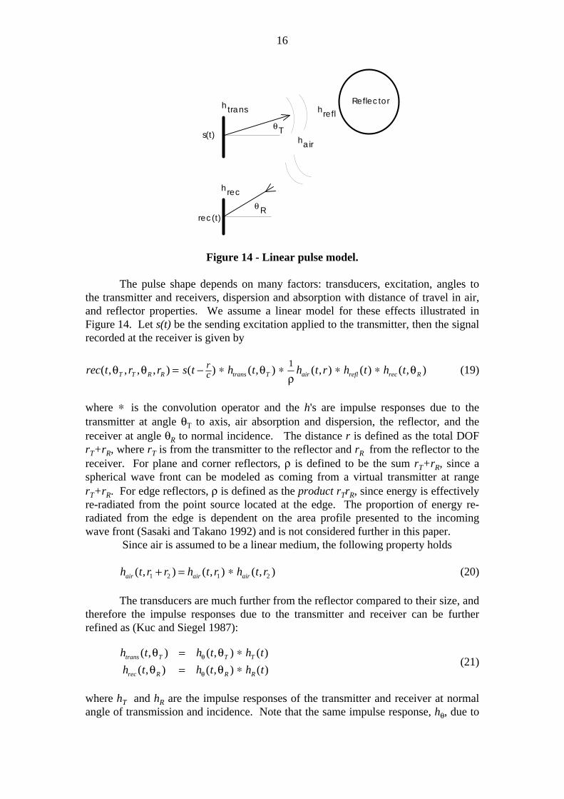
Figure 14 - Linear pulse model.

The pulse shape depends on many factors: transducers, excitation, angles tothe transmitter and receivers, dispersion and absorption with distance of travel in air,and reflector properties. We assume a linear model for these effects illustrated inFigure 14. Let s(t) be the sending excitation applied to the transmitter, then the signalrecorded at the receiver is given by

rec t r r s t h t h t r h t h tT T R R trans T air refl rec Rrc( , , , , ) ( ) ( , ) ( , ) ( ) ( , )θ θ θ

ρθ= − ∗ ∗ ∗ ∗1

(19)

where ∗ is the convolution operator and the h's are impulse responses due to thetransmitter at angle θT to axis, air absorption and dispersion, the reflector, and thereceiver at angle θR to normal incidence. The distance r is defined as the total DOFrT+rR, where rT is from the transmitter to the reflector and rR from the reflector to thereceiver. For plane and corner reflectors, ρ is defined to be the sum rT+rR, since aspherical wave front can be modeled as coming from a virtual transmitter at rangerT+rR. For edge reflectors, ρ is defined as the product rTrR, since energy is effectivelyre-radiated from the point source located at the edge. The proportion of energy re-radiated from the edge is dependent on the area profile presented to the incomingwave front (Sasaki and Takano 1992) and is not considered further in this paper.

Since air is assumed to be a linear medium, the following property holds

h t r r h t r h t rair air air( , ) ( , ) ( , )1 2 1 2+ = ∗ (20)

The transducers are much further from the reflector compared to their size, andtherefore the impulse responses due to the transmitter and receiver can be furtherrefined as (Kuc and Siegel 1987):

h t h t h t

h t h t h ttrans T T T

rec R R R

( , ) ( , ) ( )

( , ) ( , ) ( )

θ θθ θ

θ

θ

= ∗= ∗

(21)

where hT and hR are the impulse responses of the transmitter and receiver at normalangle of transmission and incidence. Note that the same impulse response, hθ, due to

17

angular dependence applies to transmitter and receiver, due to reciprocity betweentransmitter and receiver. From equations (20) and (21), equation (19) can be rewrittenas:

rec t r r ref t h t h t r r h tT T R R Tref

air ref R

r

c( , , , , ) ( ) ( , ) ( , ) ( , )θ θ θ

ρρ

θθ θ= − ∗ ∗ − ∗ (22)

where

ref t s t h t h t r h t h tTref

air ref refl R( ) ( ) ( ) ( , ) ( ) ( )= ∗ ∗ ∗ ∗1ρ

(23)

is obtained by storing a reference echo pulse from a plane5 aligned to the transmitterand receiver at a range rref/2. A typical value of rref/2 is 1 meter. For separatetransmitter and receiver, ref(t) can be obtained from a corner positioned as in Figure15. The remaining functions, hθ and hair, are determined from the transducerdiameter and calibration respectively as described in Sections 6.2 and 6.3 below. Amatrix of templates of received pulse shapes can be generated off-line for discreteangles and ranges. The appropriate range can be selected from an approximateestimate of the arrival time, and the angles chosen from the best correlation match asdescribed in Section 7.

T

R

Figure 15 - Collecting a reference pulse with separate transmitter and receiver.

6.1. Transmitted Pulse Shape

The pulse shape seen at the receiver is determined by equation (19). We havecontrol over the excitation, s(t), and the selection of transducer in determining thepulse shape. There are many different approaches to choosing the excitation - gatedsquare waves and chirps (Polaroid 1982, Sasaki and Takano 1992) and even Barkercoding (Peremans et al 1993). The main objectives are

(i) accurate TOF estimates,(ii) fine discrimination of targets,(iii) large range capability, and(iv) simplicity.

Objectives (i) and (ii) suggest a wide bandwidth pulse, and (iii) a large energy content,while (ii) suggests a narrow pulse width or a coded sequence of narrow pulses(Peremans et al 1993). A narrow pulse with large amplitude is chosen for simplicityand wide bandwidth. A wide bandwidth pulse has a sharp auto correlation peak andlow side peaks and allows a better estimate of TOF as described in Section 7.1.

5 A plane reflector was found in practice to adequately represent corners, cylinders and edges pointingtowards the sensor in terms of echo pulse shape. Pulses from edges with one plane facing away fromthe sensor are inverted in amplitude (Sasaki and Takano 1992) and are not implemented in this paper.

18

The pulse is generated by approximating an impulse applied to the transmitterwith a rectangular pulse of 10 µsec duration and 300V amplitude on a Polaroid 7000transducer. The protective cover of the transducer is removed to eliminatereverberation, thereby producing shorter cleaner pulses. The echo pulse is ACcoupled and amplified with two operational amplifiers. A typical pulse shape at 1meter from a plane reflector is shown in Figure 16. The pulse duration is 50 µsecwhich corresponds to a range discrimination of 9 mm. A narrow pulse also results ina low computational burden in the correlation calculations employed in TOFestimation.

T ime (us ec)->

0 10 20 30 40 50 60

Figure 16 - Received pulse shape from a plane reflector at 1 meter range.

6.2. Angle Dependence

The angular impulse response hθ can be obtained from the transducer shape.The received amplitude is proportion to the area exposed to the pressure impulse, andthus the response is the height profile as the impulse grazes past the surface at anangle α to the surface normal. For a circular transducer, the impulse response has theshape of the positive half of an ellipse with width equal to the propagation time acrossthe face of the transducer, tw=Dsin(|α|)/c, where D is the transducer diameter (Kucand Siegel 1987). That is

h tc

D

t

t

tt

t

otherwisew

w w

θ αα

π α( , )cos

sin,

,

= −��

− < <�

��

��

41

2

0

2

2 2 (24)

Echoes measured from a combined transmitter/receiver at angles 5o, 10o, 15o and 20o

from normal to a plane are shown in Figure 17, where good agreement betweenexperimental results and results generated from h ref hθ θ∗ ∗ can be seen. The latterechoes contain an enhanced relative level of noise due to their small amplitudes.Correlation values of 0.96 or higher are obtained between the experimental andpredicted pulse shapes over the range 0o to 20o. Moreover the best correlation matchwas within 1o of the measured angle. This suggests using the pulse shape as a meansof estimating the absolute value of the arrival angle of an echo. In practice, howeverlittle additional information is obtained from the pulse shape since the bearingestimate obtained from the arrival times of two receivers in the vector sensor is anorder of magnitude more accurate.

19

Due to the wide bandwidth of the pulse, no nulls or side-lobes occur in thetransducer angular beam pattern. This can be explained by observing that positions ofnulls and peaks in narrow band pulses are a function of frequency and thus a widebandwidth pulse adds a continuum of nulls and peaks at varying positions giving a netsmooth beam pattern. The beam pattern obtained from the energy of the pulseh ref hθ θ∗ ∗ is plotted in Figure 18. The small ripples are due to discrete time sampling

of the impulse response hθ.

T ime (us ec)

-0.2

-0.1

0

0.1

0.2

0 10 20 30 40 50 60 70

T ime (us ec)

-0.02

-0.01

0

0.01

0.02

0.03

0.04

0 10 20 30 40 50 60 70

T ime (us ec)

-0.020

-0.010

0.000

0.010

0.020

0.030

0 10 20 30 40 50 60 70

T ime (us ec)

-0.06-0.04-0.02

00.020.040.060.08

0 10 20 30 40 50 60 70

Figure 17 - Experimental and predicted echoes at 5o, 10o, 15o, 20o to transducer.

Angle (degrees )

-35

-30

-25

-20

-15

-10

-5

0

-30 -20 -10 0 10 20 30

Figure 18 - Beam pattern corresponding to the pulse shape.

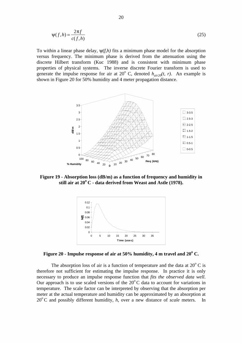
6.3. Ultrasound Absorption and Dispersion in Air

The air propagation medium absorbs sound energy as a complicated functionof temperature, humidity and frequency. Measured data (Weast and Astle 1978) ofabsorption losses of still air at 20o C are plotted in Figure 19. The same datameasurements report the speed of sound, c(f,h) against frequency, f, and humidity, h at20o C. The phase delay per meter, ψ(f,h), can be calculated as follows:

20

ψ π( , )

( , )f h

f

c f h= 2

(25)

To within a linear phase delay, ψ(f,h) fits a minimum phase model for the absorptionversus frequency. The minimum phase is derived from the attenuation using thediscrete Hilbert transform (Kuc 1988) and is consistent with minimum phaseproperties of physical systems. The inverse discrete Fourier transform is used togenerate the impulse response for air at 20o C, denoted hair20(t, r). An example isshown in Figure 20 for 50% humidity and 4 meter propagation distance.

0 10 20 30 40 50 60 70 80

Freq (kHz)

020406080100

% Humidity

0

0.5

1

1.5

2

2.5

3

3.5

dB/

m

AAAAAAAAAAAAAAAAAAAAAAAAAAAA


AAAAAAAAAAAAAAAA

AAAA

AAAAAAAAAAAAAAA


AAAAAA

AAAAAAAAAAAAAAAAAAAAAAAAAAAAAAAAAAAA


AAAAAAAAAAAAAAAAAAAA

AAAAAAAAAAA


AAAAA



AAAAAAAAAAAAAAAA

AAAAAAAAAA

AAAAAAAAAAAAAAAAAAAAAAAAAA

AAAAA



AAAAAAAAAAAA

AAA

AAAAAAAAAAAAAAA


AAAAA





AAAAA

AAAAAAAAA

AAAAAAAAAAAAAAAA

AAAA


AAAAAAA

AAAAAAAAAAAAAAAAAAAAAAAAAAAAAAAA



AAAAAAA


AAAAAAAAAAAAAAAAAAAAAAAAAAAAAA

AAAAAAAAAAAA

AAA

AAAAAAAAAAAAAAAAAAAAAAAA




AAAAAAAAA











AAAAAAAAAAAA


AAAAA


AAAAAAAAAAA





AAAAAAAAA





AAAAAAAA





AAAAAAAA





AAAAAAA

AA






AAAAAA


AA


AAAAAAAA

AAAAAA




AAA


AAAAAAAAAA

AAAAAAAA

AAA





AAA




AAAAAAAAAAAAAAAAAAAAAAAAAAAAA

AAAAA



AAAAAAAAAAAA

AAAAAAAAAAAAAAA


AAAAAA





AAAA

AAAAAAAAAAAA

AAAAAAAAAAAAAAAAAAAAAAAAAAAAAAAAAAAAAAAA


AAAAAAAAAA

AAAAAAAAAAAAAAAA

AAAAAAAA



AAAAAAA


AAAAAAAAAA


AAAAAAAAAA




AAAAAA

AAAAAAAA


AAAA



AAAAAAAAAAAAAAAA

AAAA

AAAAAAAAAAAAAAA


AAAAAA





AAAAAA


AAAAAA




AAAAAA

AAAAAAAAAAAA

AAAAAAAAAAAAAAAA

AAAA

AAAAAAAAAAAAAAAAAAAAAAAAAAAAAAAAAAAAAAAAAAAAAAAA

AAAAAAA



AAAAAAA


AAAAAAAAA

AAAAAAAAAAAA


AAAAAAAAAAA

AAAA





AAAAAA


AAAAAA


AAAAAAAAAA

AA


AAAAAAAAAA

AA



AAAAAAAA

AAAAAAAAAAAAAAAA

AAAA


AAAAAAAAAAAAA

AAAAAAAAAAAAAAAA

AAAAA







AAA



AAAAAAAAAAAAAAA


AAAAA

A

AAAAAA



AAAAAAAAAAA

AAAAAAAAAAAAAAAAAAA


AAAAAAAA

AAAAAAAAAAAAAAAAAAAAAAAAAAAAAAAAAAAAAAAAAAAAAAAAAAAA



AAAAAAAA

AAAAAAAAAAAAAAA


AAAAAAAAAAAA

AAAAAAAAAAAAAAAAAAAAAAAAAAAAAAAAAAAAAAAAA

AAA


AAAAAAAAAAAAAAAAAAAAAAAAAAAAAAAAAAAAAAAAAAAAAAAAA

AAAAAAAAAA

AAAAAAAAAAAAAAAAAAAAAAAAAAAAAAAAAAAAAAAAAAAA

AAAAAA




AAAAAAAAAA

AA



AAAAAAAA



AAAAAAA


AAAAAAAA

AAAAAA






AA

AAAAAAAAAAAA

AAA


AAAAAAAAAAA

AAAAAAAAAAAAAAAA

AAAAAAAAAAAAAAAAAAAAAAAAAAAAAAAAAAAAAAAAAAAAAAA

AAA


AAAAAAAAAAAAAAAAAAAAAAAAAAAAAAAAAAAAAAAAAAAAAAAAAAAAAAAA

AAAAAAAAAAA

AAAAAAAAAAAAAAAAAAA


AAAAAAAA

AAAAAAAAAAAAAAAAAAAAAAAAAAAAAAAAAAAAAAAAAAAAAAAAAAAA

AAAAAAAAAAAAAAAAAAAAAAAAAAAAAAAAAAAAAAAAAAAAAAAAAAAAAAAA


AAAAAAAA

AAAAAAAAAAAAAAAAAA


AAAAAAAAAAAAA

AAAAAA

AAAAAAAAAAAAAAAAAAAAAAAAAAAAAAAAAAAAAAAAAAA



AAAAAAAAAA


AAAAAAAAA


AAAAAAAAAAAAAAAAAAA



AAAAAA



AAAAAAAAAAA

AAAAAAAAAAAA








AAAAAA

AAAAAAAAAAAA



AAAAAAAA

AAAAAAAAAAAAAAA


AAAAAAAAAAAAA

AAA

AAAAAAAAAAAAAAAAAAAAAAAAAAAAAAAAAAAAAAAAAA

AA


AAAAAAAAAAAAAAAAAAAAAAAAAAAAAAAAAAAAAAAAAAAAAA

AAAAAAAAAA

AAAAAAAAAAAAAAAA


AAAAAAAA


AAAAAAAAAAAAAAAAAAAAAAAAAAAAAAAAAAAAAAAAAAAAA


AAAAAAA

AAAAAAAAAAAAAAAAAA


AAAAAAAA

AAAAAAAAAAAAAAAA

AAAA

AAAAAAAAAAAAAAAAAAAAAAAAAAAAAAAAAAAAAA


AAAAAAAAAAAA


AAAAAAAAAAAA

AA


AAAAAAAAAA


AAAAAAAAAA


AAAAAAAA


AAAAAAAA


AAAAAAA




AAAAAAAAAAAA

AAA

AAAAAA

AAA

AAAAAAAAAA


AAAAAAAA


AAAAAAAA


AAAAAA


AAAAAA



AAAAAAAAAAA

AAAAAA


AAAAAAAAAA

AAAA





AAAAAAAAA


AAAAAAA


AAAAAAA


AAAAAA


AAAAAAAAAAAA

AAA

AAAAAAAAA

AAAAAAAAAAAAAAAA

AAAA

3-3.5


AAAAA

2.5-3


AAAAA

2-2.5

AAAAAAAAAAAAAAAA

AAAA

1.5-2

AAAAAAAAAAAAAAAA

AAAA

1-1.5

AAAAAAAAAAAAAAAA

AAAA

0.5-1

0-0.5

Figure 19 - Absorption loss (dB/m) as a function of frequency and humidity instill air at 20o C - data derived from Weast and Astle (1978).

T ime (us ec)

0

0.02

0.04

0.06

0.08

0.1

0.12

0 5 10 15 20 25 30 35

Figure 20 - Impulse response of air at 50% humidity, 4 m travel and 20o C.

The absorption loss of air is a function of temperature and the data at 20o C istherefore not sufficient for estimating the impulse response. In practice it is onlynecessary to produce an impulse response function that fits the observed data well.Our approach is to use scaled versions of the 20o C data to account for variations intemperature. The scale factor can be interpreted by observing that the absorption permeter at the actual temperature and humidity can be approximated by an absorption at20o C and possibly different humidity, h, over a new distance of scale meters. In

21

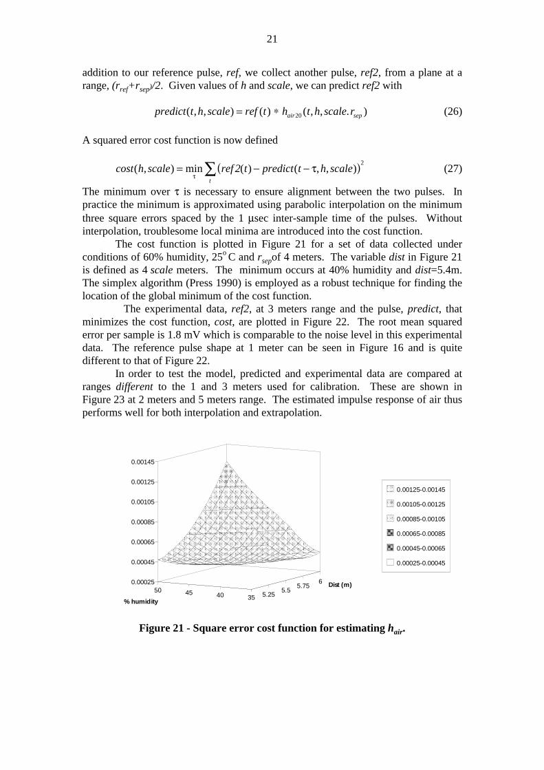
addition to our reference pulse, ref, we collect another pulse, ref2, from a plane at arange, (rref+rsep)/2. Given values of h and scale, we can predict ref2 with

predict t h scale ref t h t h scale rair sep( , , ) ( ) ( , , . )= ∗ 20 (26)

A squared error cost function is now defined

cost h scale ref 2 t predict t h scalet

( , ) min ( ) ( , , )= − −∑ττ� �2 (27)

The minimum over τ is necessary to ensure alignment between the two pulses. Inpractice the minimum is approximated using parabolic interpolation on the minimumthree square errors spaced by the 1 µsec inter-sample time of the pulses. Withoutinterpolation, troublesome local minima are introduced into the cost function.

The cost function is plotted in Figure 21 for a set of data collected underconditions of 60% humidity, 25o C and rsepof 4 meters. The variable dist in Figure 21is defined as 4 scale meters. The minimum occurs at 40% humidity and dist=5.4m.The simplex algorithm (Press 1990) is employed as a robust technique for finding thelocation of the global minimum of the cost function.

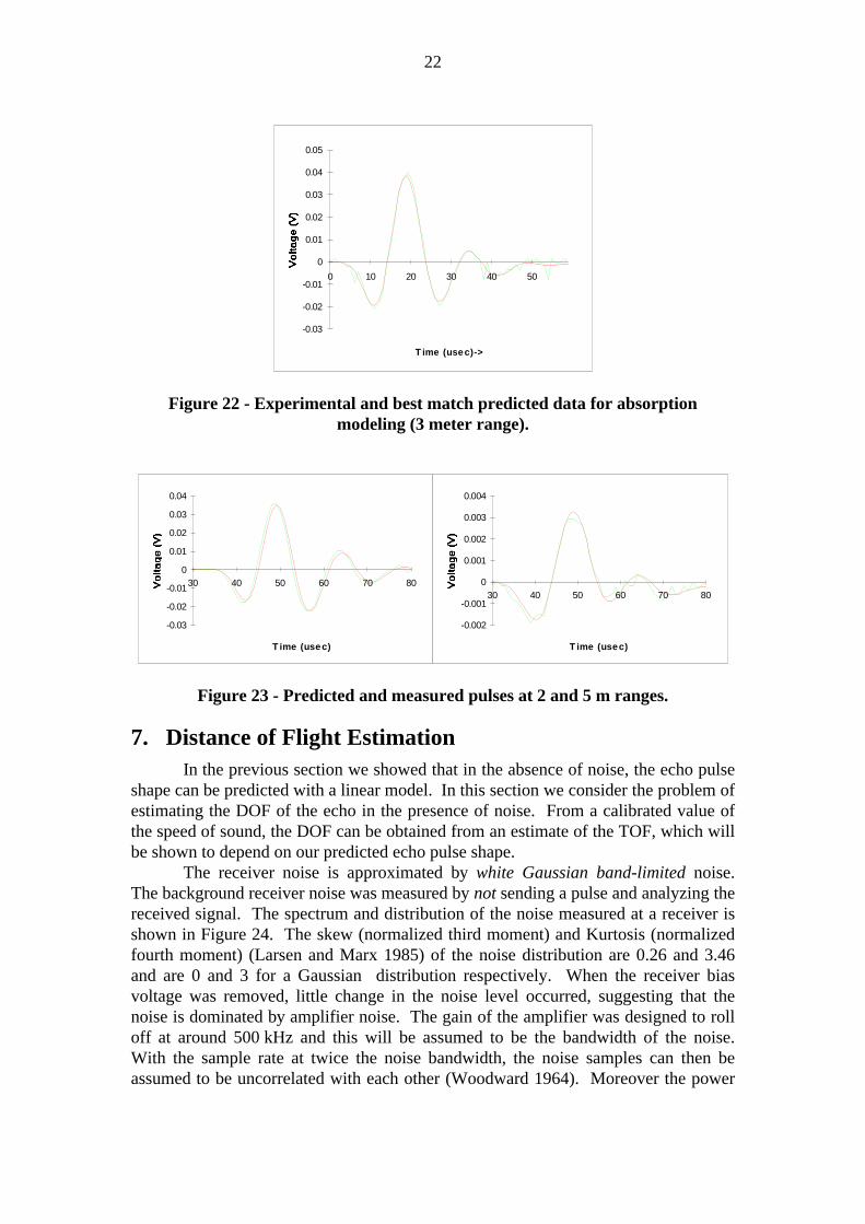
The experimental data, ref2, at 3 meters range and the pulse, predict, thatminimizes the cost function, cost, are plotted in Figure 22. The root mean squarederror per sample is 1.8 mV which is comparable to the noise level in this experimentaldata. The reference pulse shape at 1 meter can be seen in Figure 16 and is quitedifferent to that of Figure 22.

In order to test the model, predicted and experimental data are compared atranges different to the 1 and 3 meters used for calibration. These are shown inFigure 23 at 2 meters and 5 meters range. The estimated impulse response of air thusperforms well for both interpolation and extrapolation.

5.25

5.55.75

6 Dist (m)

35404550

% humidity

0.00025

0.00045

0.00065

0.00085

0.00105

0.00125

0.00145

AAAAAAAAAAAAAAAAAAAAAAAAAAAAAAAAAAAAAAAAAA









AAAAAAAAAAAAAAAA

AAAAAA


AAAAAAAA





AAAAAAAAAAAAAA


AAAAAAAAAAAAAA


AAAAAAAAAAAAAA

AAAAAAAA

AAAAAAAAAAAAAAAA


AAAAAAAAAAAAAAAA

AAAAAA

AA

AAAAAAAAAAAAAAAAAAAAAA


AAAAAAAAAAAAAAAAAA

AAAAAAAAAAAAAAAA

AAAAAAAAAAAA

AAAAAAAAAAAAAAAA

AAAAAAAAAAAA


AAAAAAAAAAAAAAA


AAAAAAAAAAAAAAA


AAAAAAAAAAAAAAA

AAAAAAAAAAAAAAAA

AAAAAAAAAAAA

AAAAAAAAAAAA

AAAAAAAAA





AAAAAA


AAAAAAAAAA

AA


AAAAAAAAAA

AA



AAAAAAAA


AAAAAAA

AAAAAA


AAAAAAA


AAAAAAAAA

AAAAAAAAAAAA



AAAAAAAAAAAAAAAAAAAAA




AAAAAAAAAAAAAAAAAA

AAAAAAAAAA

AAAAAAAAAAAAAAAA

AAAAA

AAAAAAAA

AAAAAAAAAAAAAAAA

AAAAA

AAAAAAAAAAAAAAAA

AAAAAAA

AAA

AAAAAAAAAAAAAAAAAAAAAA


AAAAAAAAAAAAAAA


AAAAAAAAAAAAAAA


AAAAAAAAAA


AAAAAAAAAA


AAAAAAAAAA

AAAAAAAAAAAAAAAA

AAAAAAAA

AAAAAAAAAAAA

AAAAAA

AAAAAAAAAAAA

AAAAAAAAAAAA

AAAAAAAA

AAAAAAAA

AAAAAAAAAAAAAAAA


AAAAAAAAAAAAAAAA





AAAAAAAAAAAAAAAA

AAAAAAAAAAAAAAAAAAAAAAAAAAAAAAAAA

AAAAAAAAAAAAAAAAAAAAAAAAAAAAAAAAAA




AAAAAAAAAAAAAA


AAAAAAAAAAAAAA


AAAAAAAAAAAA

AAAAAAAAAA

AAAAAAAAAAAAAAAA


AAAAAAAAAAAAAAAA

AAAAAA

AAAA

AAAAAAAAAAAAAAAA

AAAAAAA

AAAAAA


AAAAAAAAAAAAAAA


AAAAAAAAAAAAAAA


AAAAAAAAAAAAAAAAAA


AAAAAAAAAAAAAAA


AAAAAAAAAAAAAAA

AAAAAAAAAAAAAAAA

AAAAAAAAAAAA

AAAAAAAAAAAA

AAA

AAAAAAAAAAAA

AAA

AAAAAAAAAAAAAAAA

AAAAAAAAAAAA


AAAAAAAA

A


AAAAAAAAA

AA



AAAAAAAAAAAAAAAAAAAAAAAAAAAAAAAAAA

AAAAAAAA


AAAAAAAA


AAAAAAAA

AAAAAAAAA





AAAAAAAAAAAAAAAAAA


AAAAAAAAAAAAAAAAAA

AAAAAAAAAAAAA

AAAAAAAAAAAA

AAAA

AAAAAAAAAA

AAAAAAAAAAAA

AAAA


AAAAA

AAAAAAAAA



AAAAAAAAAAAAAAA


AAAAAAAAAAAA


AAAAAAAAAAAA


AAAAAAAAAAAA

AAAAAAAAAAAAAAAA

AAAAAAAA

AAAAAAAAAAAAAAAA

AAAAAAAA

AAAAAAAAAAAA

AAAAAAAAAAAA

AAAAAAAAAA


AAAAAAAAAAAAAAAA

AAAAAA


AAAAAAAA





AAAAAAAAAAAAAA


AAAAAAAAAAAAAA


AAAAAAAAAAAAAAAAAA

AAAAAAAAAA

AAAAAAAAAAAAAAAA


AAAAA


AAAAAAA

AA


AAAAAAAA

AAA


AAAAAAAAAAAAAAAAAA


AAAAAAAAAAAAAAAAAA


AAAAAAAAAAAAAAAAAA


AAAAAAAAAAAAAAA

AAAAAAAAAAAAAAAA

AAAAAAAAAAAA

AAAAAAAAAAAAAAAA

AAAA

AAAAAAAAAAAAAAAA

AAAA

AAAAAAAAAAAAAAAA

AA

AAAA

AAAAAAAA


AAAAAAA

AAAAAA


AAAAAAA


AAAAAAAA

AAAAAA








AAAAAAAAAA

AAAAAAAAAAAAAAAA

AAAAA

AAAAAAAA

AAAAAAAAAAAAAAAA

AAAAA


AAAAAAAAAAAAAAAAAAAAAAA

AAA


AAAAAAAAAAAAAA


AAAAAAAAAAAA


AAAAAAAAAA


AAAAAAAAAA

AAAAAAAAAAAAAAAA

AAAAAAAA

AAAAAAAAAAAA

AAAAAAAAAAAA

AAAAAA

AAAAAA

AAAAAAAA




AAAAAAAAAAAAAA





AAAAAAAAAAAAAAAA

AAAAAAAAAAAAAAAA


AAAAA


AAAAAAA

AA


AAAAAAA

AA




AAAAAAAAAAAAAAAAAA


AAAAAAAAAAAAAAA


AAAAAAAAAAAAAAA

AAAAAAAAAAAAAAAA

AAAAAAAAAAAA

AAAAAAAAAAAA

AAAAAAAA

AA

AAAAAAAAAA

AAAAAAAAAAAAAA

AAAAAAAAAA









AAAAAAAAAAAA

AAAA




AAAAAAAAAAAA


AAAAAAAAAAAA


AAAAAAAAAA


AAAAAAAAAA

AAAAAAAAAAAAAAAA

AAAAAAAAAAAAAAAA

AAAAAAAAAAAAAAAA

AAA

AAAAAAAAAAAA

AA

AAAAAAAA

AA

AAAAAAAAAAAA

AAAAAAAAA




AAAAAAA


AAAAAAA

AAAAAAAAAAAAAAAA

AAAAAAAA

AAAAAAAAAAAA



AAAAAAA


AAAAAAA


AAAAAAAAAAAAAAAAAA


AAAAAAAAAAAAAAAAAA


AAAAAAAAAAAAAAA

AAAAAAAAAAAAAAAA

AAAAAAAAAAAA

AAAAAAAAAAAAAAAA

AAAA

AAAAAAAAAAAAAAAA

AAAA

AAAAAAAAAAAAAAAA

AAAAAAAAAAAAAAAA

AAAAAAAAAAAA

AAAAAA

AAAAAAAAAAAA

AAAAAA






AAAAAAAAAAAA


AAAAAAAAAAAA


AAAAAAAAAAAA


AAAAAAAAAA

AAAAAAAAAAAAAAAA

AAAAAAAA

AAAAAAAAAAAAAAAA

AAAAAAAAAAAAAAAA

AAAAAAAAAAAA

AAAAAAAAAAAA

AAAAAAAA

AAAAAAAA

AAAAAAAAAAAA

AAA

AAAAAAAAAAAA

AAA

AAAAAAAAAAAA

AAAAAAAAA

AAAAAAAAAAAA

AAAAAAAAA


AAAAAA

AAAAAAAAAAAA







AAAAAAAAAAAAAAAAAA


AAAAAAAAAAAAAAA


AAAAAAAAAAAAAAA

AAAAAAAAAAAA

AAAAAAAAAAAA

AAA

AAAAAAAAAAAA

AAAAAAAAAAAAAAAA

AAAAAAAA

AAAAAAAAAAAAAAAA

AAAAAAAAAAAAAAAA

AAAAAAAAAAAAAAAA

AAAAAAAA

AAAAAAAAAAAAAAAA

AAAAAAAA

AAAAAAAAAAAAAAAA

AAAAAAAA


AAAAAAAAAAAA


AAAAAAAAAAAA


AAAAAAAAAAAA


AAAAAAAAAAAA



AAAAAAAAAAAA

AAAAAAAAA

AA

AAAAAAAA

AAAAAAAAAAAAAAAA

AAAAAAAAAAAA

AAA

AAAAAAAAAAAA

AAA

AAAAAAAAAAAAAAAA

AAAAAAAAAAAA

AAAAAAAAAAAAAAAA

AAAAAAAAAAAA

AAAAAAAAAAAAAAAA

AAAAAAAAAAAA


AAAAAAAAAAAAAAA


AAAAAAA

AA


AAAAAA

AAAAAAAAAAAAAAAAAAAAAAAAA

AAAAAAAAAAAAAAAAAA


AAAAAAAAAAAAAAAAAA


AAAAA


AAAAA

AAAAAAAAAAAA

AAAAAAAAAAAA

AAA

AAAAAA

AAAAAAAAAAAAAAAAAAAAAAAAAAA

AAAAAAAAAAAAAAAA

AAAAAAAA

AAAAAAAAAAAAAAAA

AAAAAAAA

AAAAAAAAAAAAAAAA

AAAAAAAA


AAAAAAAAAA


AAAAAAAAAA






AAAAAAAAAA

AAAAAAAAAAAAAAAA

AAAAAAAAAAAAAAAA

AAAAAAAAAAAAAA

AAAAAAAAA

AAAAAAAAAAAA

AAA

AAAAAAAAAAAA

AAAAAAAAAAAAAAAA

AAAA

AAAAAAAAAAAAAAAA

AAAA

AAAAAAAAAAAAAAAA

AAAAAAAAAAAA

AAAAAAAAAAAAAAAA

AAAAAAAAAAAA


AAAAAAAAAAAAAAA


AAAAAAAAAAAAAAA


AAAAAAAAA


AAAAAA

A



AAAAAAAA


AAAAAA


AAAAAA



AAAAAAAAAAAA

AAAAAAAAAAAA

AAAA

AAAAAAAA

AAAAAAAAAAAAAAAA

AAAAAAAAAAAA

AAAAAAAAAAAA

AAAAAAAAAAAAAAAA

AAAAAAAA

AAAAAAAAAAAA

AAAAAA

AAAAAAAAAAAAAAAA

AAAAAAAA


AAAAAAAAAA


AAAAAAAAAAAA






AAAAAAAAAAAAAAAA


AAAAAAAAAAAAAAAA

AAAAAAAAAAAAAAAAAAAAAAAAAAAAAAAAAAAAAAA

AAAAAAAAAAAAAAAAAAAAAAAAAAAAAAAAAAAAAAA


AAAAA

0.00125-0.00145

AAAAAAAAAAAAAAAA

AAAA

0.00105-0.00125


AAAAA

0.00085-0.00105


AAAAA

0.00065-0.00085

AAAAAAAAAAAAAAAA

AAAA

0.00045-0.00065

0.00025-0.00045

Figure 21 - Square error cost function for estimating hair.

22

T ime (us ec)->

-0.03

-0.02

-0.01

0

0.01

0.02

0.03

0.04

0.05

0 10 20 30 40 50

Figure 22 - Experimental and best match predicted data for absorptionmodeling (3 meter range).

T ime (us ec)

-0.03

-0.02

-0.01

0

0.01

0.02

0.03

0.04

30 40 50 60 70 80

T ime (us ec)

-0.002

-0.001

0

0.001

0.002

0.003

0.004

30 40 50 60 70 80

Figure 23 - Predicted and measured pulses at 2 and 5 m ranges.

7. Distance of Flight EstimationIn the previous section we showed that in the absence of noise, the echo pulse

shape can be predicted with a linear model. In this section we consider the problem ofestimating the DOF of the echo in the presence of noise. From a calibrated value ofthe speed of sound, the DOF can be obtained from an estimate of the TOF, which willbe shown to depend on our predicted echo pulse shape.

The receiver noise is approximated by white Gaussian band-limited noise.The background receiver noise was measured by not sending a pulse and analyzing thereceived signal. The spectrum and distribution of the noise measured at a receiver isshown in Figure 24. The skew (normalized third moment) and Kurtosis (normalizedfourth moment) (Larsen and Marx 1985) of the noise distribution are 0.26 and 3.46and are 0 and 3 for a Gaussian distribution respectively. When the receiver biasvoltage was removed, little change in the noise level occurred, suggesting that thenoise is dominated by amplifier noise. The gain of the amplifier was designed to rolloff at around 500 kHz and this will be assumed to be the bandwidth of the noise.With the sample rate at twice the noise bandwidth, the noise samples can then beassumed to be uncorrelated with each other (Woodward 1964). Moreover the power

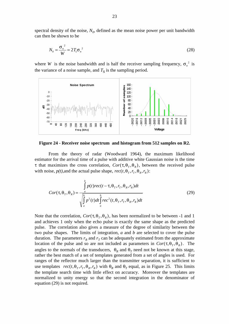
23

spectral density of the noise, N0, defined as the mean noise power per unit bandwidthcan then be shown to be

NW

Tns n0

222= =σ σ (28)

where W is the noise bandwidth and is half the receiver sampling frequency, σn2 is

the variance of a noise sample, and Ts is the sampling period.

Noise S pectrum

F req (kH z)

-70

-60

-50

-40

-30

-20

-10

0

Voltage

020406080

100120140160

Figure 24 - Receiver noise spectrum and histogram from 512 samples on R2.

From the theory of radar (Woodward 1964), the maximum likelihoodestimator for the arrival time of a pulse with additive white Gaussian noise is the timeτ that maximizes the cross correlation, Cor T R( , , )τ θ θ , between the received pulsewith noise, p(t),and the actual pulse shape, rec t r rT T R R( , , , , )θ θ :

Cor

p t rec t r r dt

p t dt rec t r r dt

T R

T T R R

a

b

a

b

T T R R

a

b( , , )

( ) ( , , , , )

( ) ( , , , , )

τ θ θτ θ θ

θ θ

=−�

� �2 2

(29)

Note that the correlation, Cor T R( , , )τ θ θ , has been normalized to be between -1 and 1and achieves 1 only when the echo pulse is exactly the same shape as the predictedpulse. The correlation also gives a measure of the degree of similarity between thetwo pulse shapes. The limits of integration, a and b are selected to cover the pulseduration. The parameters rR and rT can be adequately estimated from the approximatelocation of the pulse and so are not included as parameters in Cor T R( , , )τ θ θ . Theangles to the normals of the transducers, θR and θT need not be known at this stage,rather the best match of a set of templates generated from a set of angles is used. Forranges of the reflector much larger than the transmitter separation, it is sufficient touse templates rec t r rT T R R( , , , , )θ θ with θR and θT equal, as in Figure 25. This limitsthe template search time with little effect on accuracy. Moreover the templates arenormalized to unity energy so that the second integration in the denominator ofequation (29) is not required.

24

Angle(degrees )

0.60

0.65

0.70

0.75

0.80

0.85

0.90

0.95

1.00

0 2 4 6 8 10 12 14 16 18 20

Figure 25 - Measured correlation against θθR =θθT for a plane at 10o inclination totransmitter and receiver.

In practice, discrete time versions of the signals are only available and soCor T R( , , )τ θ θ is evaluated at discrete times (1 µsec apart in our sensor) withsummations rather than the integrals. To achieve sub-sample resolution, parabolicinterpolation is performed on the maximum three samples of Cor T R( , , )τ θ θ to find abetter estimate of the position of the maximum. If the three maxima y0, y1, and y2occur at integer sample numbers 0,1 and 2, the parabolic estimate of the position ofthe maximum is

maxposy y y

y y y= − +

− +2 1 0

2 1 0

4 32 2( )

(30)

7.1. Distance of Flight Jitter

The estimate of DOF described above inevitably has errors due to receivernoise and actual physical variations in the TOF due to random properties of air, suchas turbulence, local temperature fluctuations and gradients. These DOF estimateerrors, called jitter here, need to be characterized so that the level of confidence ofmeasurements and reflector discrimination can be determined.

We start by examining the jitter attributed to receiver noise. From Woodward(1964), when the energy of a pulse, E, is much larger than the noise power spectraldensity, N0 , the standard deviation of the correlation estimate of arrival time, σR, is

σR B

N

E= 1

20 (31)

where Β is the bandwidth of the pulse defined by the normalized second moment ofthe pulse power spectrum:

BF f f df

F df=

−��

2

20

2

2π

( ) (32)

where F is the Fourier transform of the pulse, f is frequency and f0 is the centroid ofthe power spectrum defined by:

25

fF f df

F df0

2

2= ��

(33)

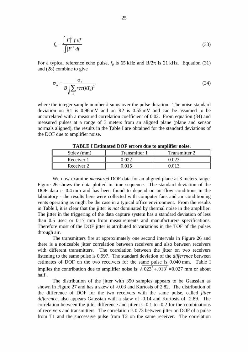
For a typical reference echo pulse, f0 is 65 kHz and Β/2π is 21 kHz. Equation (31)and (28) combine to give

σ σR

n

sk

B rec kT=

∑ ( )2 (34)

where the integer sample number k sums over the pulse duration. The noise standarddeviation on R1 is 0.96 mV and on R2 is 0.55 mV and can be assumed to beuncorrelated with a measured correlation coefficient of 0.02. From equation (34) andmeasured pulses at a range of 3 meters from an aligned plane (plane and sensornormals aligned), the results in the Table I are obtained for the standard deviations ofthe DOF due to amplifier noise.

TABLE I Estimated DOF errors due to amplifier noise.Stdev (mm) Transmitter 1 Transmitter 2Receiver 1 0.022 0.023Receiver 2 0.015 0.013

We now examine measured DOF data for an aligned plane at 3 meters range.Figure 26 shows the data plotted in time sequence. The standard deviation of theDOF data is 0.4 mm and has been found to depend on air flow conditions in thelaboratory - the results here were collected with computer fans and air conditioningvents operating as might be the case in a typical office environment. From the resultsin Table I, it is clear that the jitter is not dominated by thermal noise in the amplifier.The jitter in the triggering of the data capture system has a standard deviation of lessthan 0.5 µsec or 0.17 mm from measurements and manufacturers specifications.Therefore most of the DOF jitter is attributed to variations in the TOF of the pulsesthrough air.

The transmitters fire at approximately one second intervals in Figure 26 andthere is a noticeable jitter correlation between receivers and also between receiverswith different transmitters. The correlation between the jitter on two receiverslistening to the same pulse is 0.997. The standard deviation of the difference betweenestimates of DOF on the two receivers for the same pulse is 0.040 mm. Table I

implies the contribution due to amplifier noise is . .023 0132 2+ =0.027 mm or abouthalf .

The distribution of the jitter with 350 samples appears to be Gaussian asshown in Figure 27 and has a skew of -0.03 and Kurtosis of 2.82. The distribution ofthe difference of DOF for the two receivers with the same pulse, called jitterdifference, also appears Gaussian with a skew of -0.14 and Kurtosis of 2.89. Thecorrelation between the jitter difference and jitter is -0.1 to -0.2 for the combinationsof receivers and transmitters. The correlation is 0.73 between jitter on DOF of a pulsefrom T1 and the successive pulse from T2 on the same receiver. The correlation

26

between jitter differences on successive transmitters is 0.45. Therefore the covariancematrix R of Section 5.4 has significant off-diagonal elements. Correlationcoefficients for experimental data at other DOFs are plotted in Figure 30. These arediscussed in the next section.

The results above can be explained by local variations of the speed of soundslow enough to show correlation after times in the order of seconds. The spatialcorrelation of the speed of sound variations is high compared to the receiver spacing.This is necessary for high bearing accuracy with closely spaced receivers. Theseeffects are most likely caused by the slow mixing of air of different temperatures, likea cold draft on a Winter's night. The increased fluctuation of DOF with increased airflow observed in the laboratory is consistent with this view. Other authors havereported similar results (Brown 1985 and Peremans 1993).

Figures 28 and 29 show the standard deviation of 400 samples of measuredDOF and difference in DOF for a range of 0.5 m to 5 m of an aligned plane. Thestandard deviation at DOF less than 2 meters is mostly due to the data capturetriggering component of 0.17 mm as discussed above. This data shows the effect ofdistance in the jitter of measurements and it can be seen that the jitter is somewhatspurious due to local air currents in the laboratory. The difference jitter in Figure 29shows a more definite trend with distance. The difference jitter due to the amplifiernoise is shown as the solid line and approaches the actual difference jitter as the rangeincreases due to declining signal to noise ratio.

Distance of flight

Sample

me

ters

5.995

6.000

6.005

6.010

1 51 101 151 201 251 301

Figure 26 - Measured DOF against sample for an aligned plane at 3 metersrange. The top two traces are from transmitter T1 with receivers R1 and R2,

and the bottom two closely spaced traces are T2 with R1 and R2.

27

Dis tance of F light E rror His togram

Dis tance error

0

5

10

15

20

25

30

35

40

45

Figure 27 - Measured distribution of DOF and Gaussian distribution with samestandard deviation.

DOF (m)

Sta

nd d

ev

DO

F (m

)

0

0.0001

0.0002

0.0003

0.0004

1 2 3 4 5 6 7 8 9 10

T2

T1

T1model

Figure 28 - Standard deviation of measured DOF (400 samples each meter) andmodel for an aligned plane.

28

DOF (m)

Sta

nd D

ev

Diff

ere

nce

in D

OF

(m)

0.00E+00

2.00E-05

4.00E-05

6.00E-05

8.00E-05

1 2 3 4 5 6 7 8 9 10

Diff2

Diff1

diff_amp

Diff1_model

Figure 29 - Standard deviation of measured difference in DOF for an alignedplane (triangles from T1, squares from T2) and the estimate amplifier noise (line)from measured echo energy, bandwidth and a fitted noise spectral density. The

dashed line is that used in the model.

DOF (m)

Co

rre

latio

n C

oe

ffic

ient

s

-0.1

0

0.1

0.2

0.3

0.4

0.5

0.6

1 2 3 4 5 6 7 8 9 10

T1T2

T1T2_model

Diff1Diff2

Diff1Diff2_model

T1Diff1

T1diff1_model

T2Diff2

T2Diff2_model

Figure 30 - Significant correlation coefficients of measurements and model for analigned plane.

7.2. A Model for Distance of Flight and Bearing Errors

A simple model is presented for the standard deviation of the DOF and bearingestimates of the sensor. The model is employed for the statistical discrimination ofplanes, corners and edges presented in Section 5.4. We consider three contributions.The first contribution, nair, is due to fluctuations in the speed of sound, and thesecond, ntrig, is due to jitter in the data capture triggering. The third contribution,namp, is due to the amplifier noise and is estimated from known pulse and amplifiernoise characteristics. The noise in the DOF from transmitter T (1 or 2) and receiver R(1 or 2) is denoted by ndofTR

29

ndof nair ntrig nampTR TR TR TR= + + (35)

and is described in terms of noise variables n's which are each independent, zeromean, Gaussian, unity variance random variables:

nair k k k kTR air a alocalR

diff difflocal= + + − +−σ n n n na aT diff diffT( ) ( )1 1 �

ntrig k kTR trig trigR

trigdiff= + − −σ n ntrigT trigdiffT( )1 1 �nampTR ampTR= σ nampTR (36)

where the k's are fixed constants defined to have a sum of squares of 1 within eachcontribution so that nair's and ntrig's all have variances σair

2 and σtrig2. Each term in

equation (36) has a physical explanation. The terms kana and kdiffndiff are due to thejitter and jitter difference common to all four DOF measurements. The kalocalnaT andkdifflocalndiffT terms account for correlation between receiver measurements taken at thesame time. The ktrigntrigT is the jitter in triggering the data capture system common toboth receivers and ktrigdiffntrigdiffT is the trigger jitter in the difference of the receivers.The σampTRnampTR term is the independent contribution due to amplifier noise on eachreceiver/transmitter combination and σampTR is obtained from cσR in equation (34) andis a function of the amplifier noise, pulse energy and bandwidth, all of which areknown by the sensor software.

The jitter variance attributed to air, σair, is assumed to be proportional to theDOF, dof

σ σair adof2 2= (37)

This makes the reasonable assumption that the air path is composed of manyindependent jitter elements whose net sum is the overall contribution.

From equation (36) we can evaluate the variances of the DOF

σ σ σ σndof air trig ampTT1

2 2 21

2= + + (38)

From equation (8), the bearing noise, nαT and its noise variance,σ αn T

2 from transmitter

T is given by

nk k k

d

k k k

d

T

air diff difflocal trig trigdiff ampT ampT

nair diff difflocal trig trigdiff ampT ampT

T

α

α

σ σ σ σ

σσ σ σ σ

=+ + + −

=+ + + +

2 2

4 4

1 2

22 2 2 2 2

12

22

2

n n n n ndiff diffT trigdiffT ampT 1 ampT 2 �

( )

(39)

The covariance matrix R of the measurement noise vector [ndof11 nα1 ndof21 nα2]T isgiven by

30

R =

�

�

�

��

σ σ σ σσ σ σ σσ σ σ σσ σ σ σ

α α

α α α α α

α α

α α α α α

ndof ndof n ndof ndof ndof n

ndof n n ndof n n n

ndof ndof ndof n ndof ndof n

ndof n n n ndof n n

11 11 1 11 21 11 2

11 1 1 21 1 1 2

11 21 21 1 21 21 2

11 2 1 2 21 2 2

2

2

2

2

(40)

Each of these components is a simple function of σ's, k's and d:

σσ σ σ

αndof nair diff difflocal trig trigdiff ampk k k

d11 1

2 22 2 2 2 211

2

=+ + +( )

(41)

σ σndof ndof air a diffk k11 21

2 2 2= +( ) ,σσ

αndof nair diffk

d11 2

2 2 2

= ,σσ

αndof nair diffk

d21 1

2 2 2

= ,σσ

α αn nair diffk

d1 2

4 2 2

2=

σσ σ σ

αndof nair diff difflocal trig trigdiff ampk k k

d21 2

2 22 2 2 2 221

2

=+ + +( )

The above model has been fitted, using a spreadsheet with trial and error, tothe experimental data in Figures 28, 29 and 30, and reasonable agreement has beenobtained. The following values have been employed:

σ

σa a alocal diff

difflocal trig trigdiff trig

m k k k

k m k k

= = = =

= = = =

0 0001 0 83 0 55 0 044

0 01 0 00017 0 04 0 9992

0 5. , . , . , .

. , . , . , .

.

The values of half of the constants are approximately independent of air conditionsexperienced in the laboratory. Over four experiments under varying air conditions, thefollowing constants varied significantly:

σa a

alocal diff

m k

k k

= − = −= − = −0 00008 0 0003 0 83 0 93

0 35 0 55 0 023 0 049

0 5. . , . . ,

. . , . .

.

A calibration procedure may be necessary in practice if high precision error estimatesare required by an application.

The experimental results for an aligned plane have been presented to show thejitter effects due to the air propagation medium. More generally, the covariancematrix for off-axis planes and other reflectors share the same air propagation and datacapture jitter characteristics but have different components due to amplifier noise,since the bandwidth and energy of the pulses are dependent on the angle oftransmission and reception and reflector efficiency. Since the bandwidth and energyare easily predicted from our linear model, we can estimate our covariance matrix Rfor all received pulses. The bandwidth versus range and angle is plotted in Figure 31.Note that as bandwidth decreases, the amplifier noise contribution to the jitterincreases and the overall error becomes less correlated as a result.

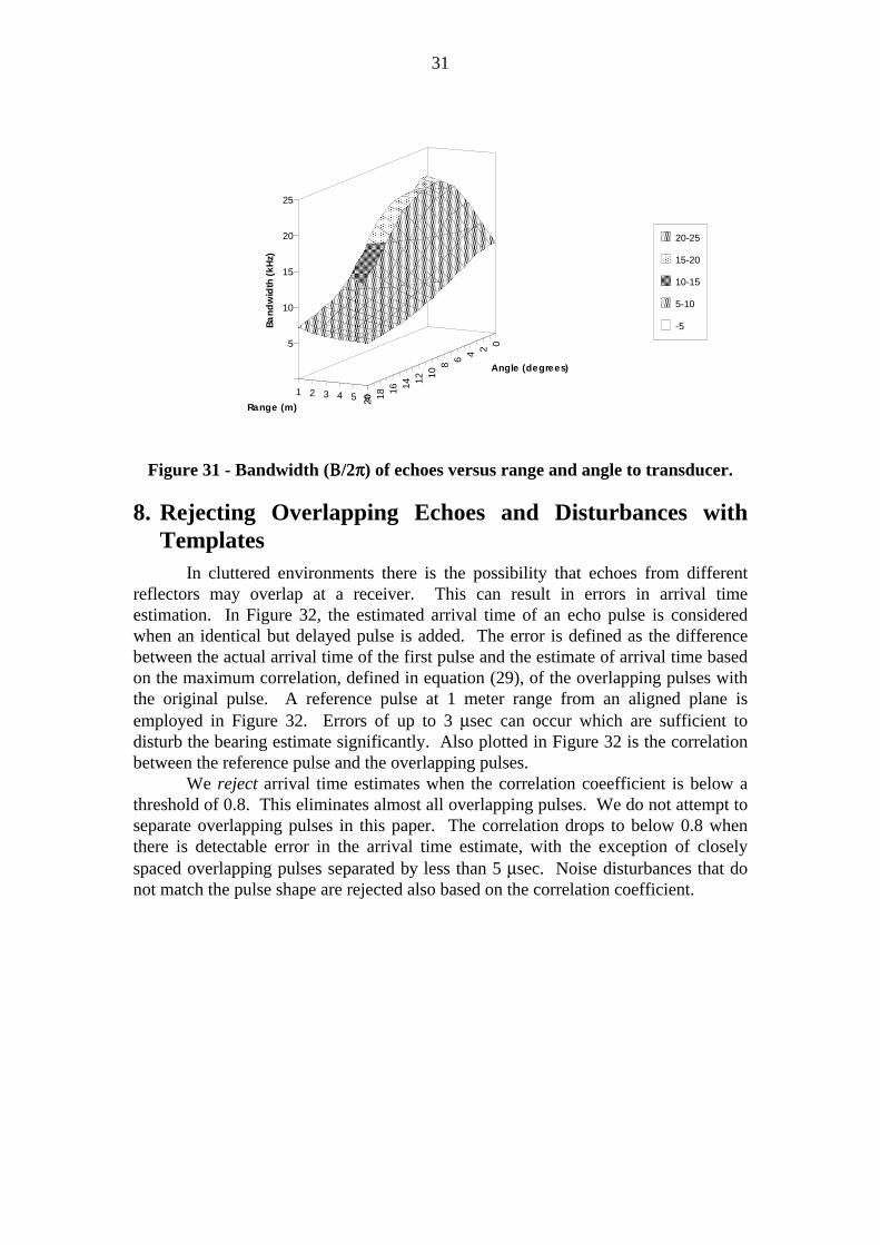
31

02468101214161820

Angle (degrees)

1 2 3 4 5 6Range (m)

5

10

15

20

25

Band

wid

th (

kHz)

AAAAAAAAAAAAAAAA

AAAAAAAAAAAAAAAA

AAAA


AAAAA

AAAAAAAAAAAAAAAA

AAAAAAAA


AA

AAAAAAAA

AAAA

AAAAAAAAAAAA

AAA

AAAAAAAA

AAAAAAAAAAAAAAAA

AAAAAAAAAAAAAAAA

AAAA

AAAAAAAAAAAAAAAA

AAAAAAAAAAAAAAAA





AAAAAAAAAAAA


AAAAAAAAAAAAAAAA

AAAAAAAA


AAAAAAAA


AAAAAAAAAAAAAAAAAA

AAAA


AAAAAAAAAAAA

AAAAAAAA





AAAAAAAAAAAA


AAAAAAAAAAAA


AAAAAA


AAAAAAAAAAAAA

AAA


AAAAAAAA

AAA





AAAAA









AAAAA

AAAAAAAA

AAAAAAAA

AAAAAA

AAAAAAAAA

AAAAAAAAAAAA

AAAAAAAAAAAAAAAA

AAAAAAAAAAAA

AAA

AAAAAAAAAAAAAAAA

AAAAAAAA

AAAAAA

AAAAAAAAAAAAAAAA

AAAA

AAAAAAAAAAAA

AAAAAAAAAAAAAAAA

AAAAAAA

AAA


AAAAAAAAAAAAAA

AA


AAAAAAAAAAAAAA

AA







AAAAAAAAAAAAAAAA


AAAAAAA


AAAAAAAAAAAAAA


AAAAAAAAAAAAAAAAAAA

AAAAAA


AAAAAAAAAAAA

AAAAAAAA





AAAAAAAAA


AAAAAAAAAAAAAA

AAAAAA


AAAAAAAAAAAAAA

AAAAAAAAAAAAAAAA

AAAAAAAAAAA

AAAAAA


AAAAA

AAAAAAAAAAAA











AAAAAAAAAAAAAAAA

AAAAAAAAAAAAAAAA

AAAAAAAAAAAAAAAA

AAAAAAAAAAAAAAAA









AAAAAAAAAA



AAAAAAAA


AAAAAAAA

AAAAAAAAAAAA


AAAAAAAAAAAAAAAA


AAAAAAAAAAA



AAAAAAAAAAA


AAAAAA



AAAA


AAAAAAAAAA

AA





AAAAAAAA


AAAAAAAAAAAA

AAAAAAAAAA


AAAAAAAAAAAA


AAAAAAAAAAAAAA

AAAAAAAA


AAAAAAAAA

AAAAAAAA

AAA







AAAAA

AAAAAAAAAAAAAAAA

AAAAAAAAAAAAAAAA

AAAAAAAAAAAAAAAA

AAAAAAAAAAAAAAAA

AAAAAAAAAAAAAAAA

AAAAAAAAAAAAAAAA

AAAAAAAAAAAA

AAAAAAAAAAAA

AAA

AAAAAAAAAAAAAAAA

AAAAAAAAAAAAAAAA



AAAAAA


AAAAAAAAAA

AAAAAAAAA



AAAAAA


AAAAAAAAAAAAAAAA

AAAAAAAAAAAAAAAA


AAAAAAA



AAAAAAA



AAAAAAAAAAAAAA


AAAAAAAAAAAAAAAAAA

AAAAAAAAAAAAAAAA


AAAAAAAA

AAAAAAAAAAAAAAA


AAAAAAAAAAAAAAAAAAA


AAAAAAAAAAAAAAAAAAA



AAAAAAAAAA





AAAAAAAAAAAAAAAA

AAAAAAAA

AAAAAAAAAAAAAAAA

AAAAA

AAAAAAAAAAAAAAAA

AAAAAAAA

AAAAAAAAAAAAAAAA

AAAAAAAAAA


AAAAAAAAAA

AAAA


AAAAAAAAAA

AAAA









AAAAAAAAAAAA

AAAAAAAAAAAA

AAAAAAAAAAAAAAAA

AAAAAAAAAAAAAAAA

AAAAAAAAAAAAAAAA

AAAAAAAAAAAAAAAA

AAAAAAAAAAAA

AAAAAAAAAAAA

AAAAAAAAAAAA

AAAAAAAAAAAA


AAAAAAAAAAAAAAAA

AAAAAA


AAAAAAAAAAAAAAAAA



AA


AAAAAAAAAAAAAAAAAAA

A



AAAAAAAA







AAAAAA


AAAAAAAAAAAAAAAA

AAAAAA


AAAAAAAA

AAAAAAAAAAAAA


AAAAAA

AAAAAAAAAAAAAAAA


AAAAAAAAAAAA


AAAAAAAAAA

AAAAAAAAAAAAAAAA


AAAAAAAAA

AAAAAAAA


AAAAAAAAAAAAA


AAAAAAAAAAAAA







AAAAAAAAAAAAAAAA

AAAAAAAAAAAAAAAA

AAAA

AAAAAAAAAAAAAAAA

AAAAAAAAAAAAAAAA

AAAAAAAAAAAAAAAA

AAAAAAAAAAAAAAAA

AAAAAAAAAAAAAAAA

AAAAAAAAAAAAAAAA

AAAAAAAAAAAA

AAAAAAAAAAAA

AAA

AAAAAAAAAAAAAAAA

AAAAAAAAAAAAAAAA

AAAAAAAAAAAA

AAAAAAAAAAAA

AAAAAAAAAAAAAAAA

20-25


15-20

AAAAAAAAAAAAAAAA

10-15

AAAAAAAAAAAAAAAA

5-10

-5

Figure 31 - Bandwidth (ΒΒ/2ππ) of echoes versus range and angle to transducer.

8. Rejecting Overlapping Echoes and Disturbances withTemplates

In cluttered environments there is the possibility that echoes from differentreflectors may overlap at a receiver. This can result in errors in arrival timeestimation. In Figure 32, the estimated arrival time of an echo pulse is consideredwhen an identical but delayed pulse is added. The error is defined as the differencebetween the actual arrival time of the first pulse and the estimate of arrival time basedon the maximum correlation, defined in equation (29), of the overlapping pulses withthe original pulse. A reference pulse at 1 meter range from an aligned plane isemployed in Figure 32. Errors of up to 3 µsec can occur which are sufficient todisturb the bearing estimate significantly. Also plotted in Figure 32 is the correlationbetween the reference pulse and the overlapping pulses.

We reject arrival time estimates when the correlation coeefficient is below athreshold of 0.8. This eliminates almost all overlapping pulses. We do not attempt toseparate overlapping pulses in this paper. The correlation drops to below 0.8 whenthere is detectable error in the arrival time estimate, with the exception of closelyspaced overlapping pulses separated by less than 5 µsec. Noise disturbances that donot match the pulse shape are rejected also based on the correlation coefficient.

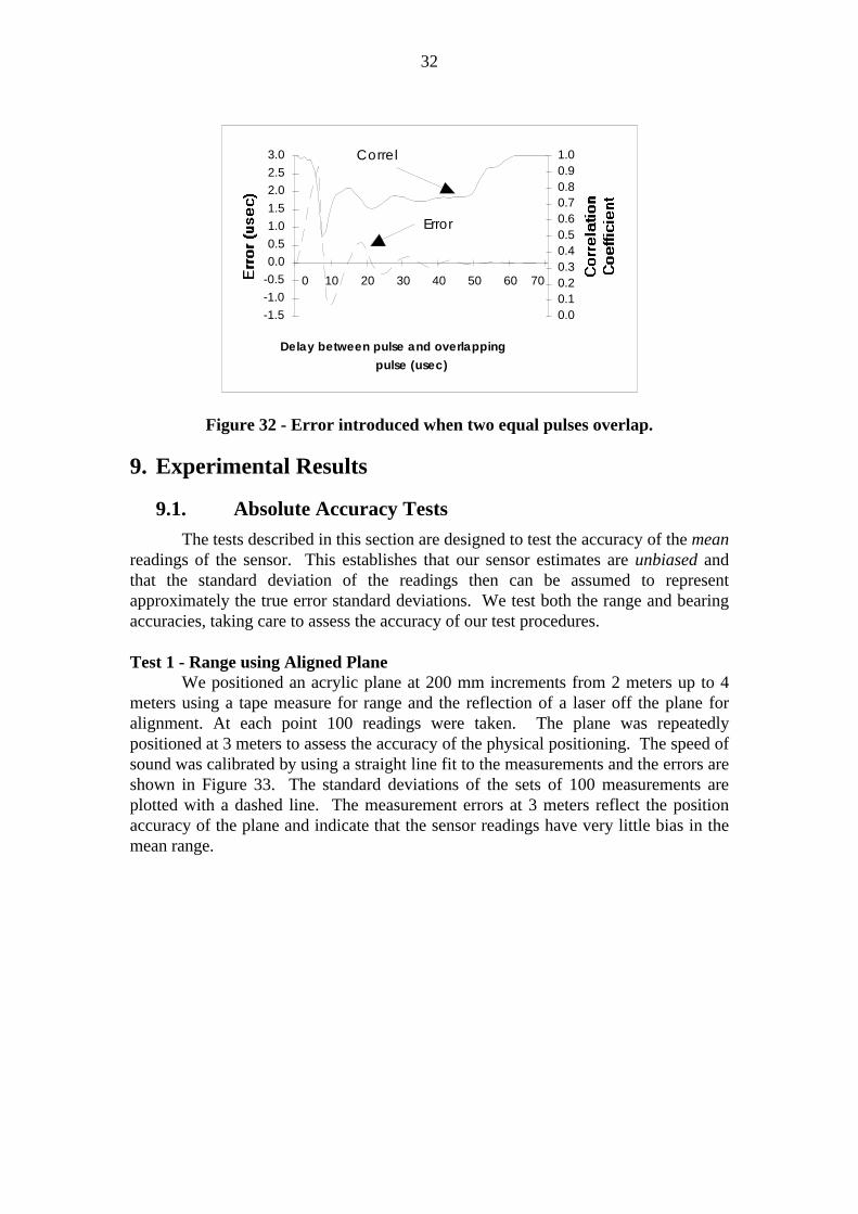
32

Delay between pulse and overlappingpulse (usec)

-1.5

-1.0

-0.5

0.00.5

1.0

1.5

2.02.5

3.0

0 10 20 30 40 50 60 70

0.00.10.20.30.40.50.60.70.80.91.0Correl

Error

Figure 32 - Error introduced when two equal pulses overlap.

9. Experimental Results

9.1. Absolute Accuracy Tests

The tests described in this section are designed to test the accuracy of the meanreadings of the sensor. This establishes that our sensor estimates are unbiased andthat the standard deviation of the readings then can be assumed to representapproximately the true error standard deviations. We test both the range and bearingaccuracies, taking care to assess the accuracy of our test procedures.

Test 1 - Range using Aligned PlaneWe positioned an acrylic plane at 200 mm increments from 2 meters up to 4

meters using a tape measure for range and the reflection of a laser off the plane foralignment. At each point 100 readings were taken. The plane was repeatedlypositioned at 3 meters to assess the accuracy of the physical positioning. The speed ofsound was calibrated by using a straight line fit to the measurements and the errors areshown in Figure 33. The standard deviations of the sets of 100 measurements areplotted with a dashed line. The measurement errors at 3 meters reflect the positionaccuracy of the plane and indicate that the sensor readings have very little bias in themean range.

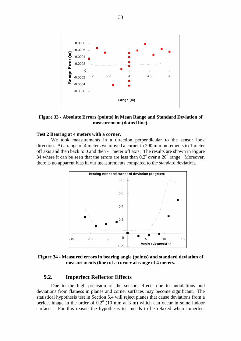
33

Range (m)

-0.0006

-0.0004

-0.0002

0

0.0002

0.0004

0.0006

0.0008

2.5 3 3.5 42

Figure 33 - Absolute Errors (points) in Mean Range and Standard Deviation ofmeasurement (dotted line).

Test 2 Bearing at 4 meters with a corner.We took measurements in a direction perpendicular to the sensor look

direction. At a range of 4 meters we moved a corner in 200 mm increments to 1 meteroff axis and then back to 0 and then -1 meter off axis. The results are shown in Figure34 where it can be seen that the errors are less than 0.2o over a 20o range. Moreover,there is no apparent bias in our measurements compared to the standard deviation.

Angle (degrees) ->

Bearing error and standard deviation (degrees)

-0.2

0

0.2

0.4

0.6

0.8

-15 -10 -5 5 10 15

Figure 34 - Measured errors in bearing angle (points) and standard deviation ofmeasurements (line) of a corner at range of 4 meters.

9.2. Imperfect Reflector Effects

Due to the high precision of the sensor, effects due to undulations anddeviations from flatness in planes and corner surfaces may become significant. Thestatistical hypothesis test in Section 5.4 will reject planes that cause deviations from aperfect image in the order of 0.2o (10 mm at 3 m) which can occur in some indoorsurfaces. For this reason the hypothesis test needs to be relaxed when imperfect

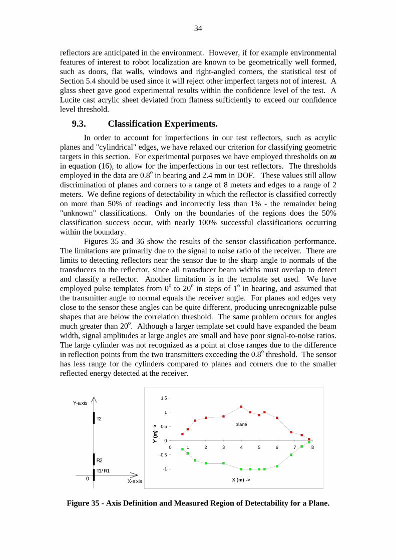
34

reflectors are anticipated in the environment. However, if for example environmentalfeatures of interest to robot localization are known to be geometrically well formed,such as doors, flat walls, windows and right-angled corners, the statistical test ofSection 5.4 should be used since it will reject other imperfect targets not of interest. Aglass sheet gave good experimental results within the confidence level of the test. ALucite cast acrylic sheet deviated from flatness sufficiently to exceed our confidencelevel threshold.

9.3. Classification Experiments.

In order to account for imperfections in our test reflectors, such as acrylicplanes and "cylindrical" edges, we have relaxed our criterion for classifying geometrictargets in this section. For experimental purposes we have employed thresholds on min equation (16), to allow for the imperfections in our test reflectors. The thresholdsemployed in the data are 0.8o in bearing and 2.4 mm in DOF. These values still allowdiscrimination of planes and corners to a range of 8 meters and edges to a range of 2meters. We define regions of detectability in which the reflector is classified correctlyon more than 50% of readings and incorrectly less than 1% - the remainder being"unknown" classifications. Only on the boundaries of the regions does the 50%classification success occur, with nearly 100% successful classifications occurringwithin the boundary.

Figures 35 and 36 show the results of the sensor classification performance.The limitations are primarily due to the signal to noise ratio of the receiver. There arelimits to detecting reflectors near the sensor due to the sharp angle to normals of thetransducers to the reflector, since all transducer beam widths must overlap to detectand classify a reflector. Another limitation is in the template set used. We haveemployed pulse templates from 0o to 20o in steps of 1o in bearing, and assumed thatthe transmitter angle to normal equals the receiver angle. For planes and edges veryclose to the sensor these angles can be quite different, producing unrecognizable pulseshapes that are below the correlation threshold. The same problem occurs for anglesmuch greater than 20o. Although a larger template set could have expanded the beamwidth, signal amplitudes at large angles are small and have poor signal-to-noise ratios.The large cylinder was not recognized as a point at close ranges due to the differencein reflection points from the two transmitters exceeding the 0.8o threshold. The sensorhas less range for the cylinders compared to planes and corners due to the smallerreflected energy detected at the receiver.

X-axis

Y-axis

0

T2

R2

T1/R1

X (m) ->

-1

-0.5

0

0.5

1

1.5

0 1 2 3 4 5 6 7 8

plane

Figure 35 - Axis Definition and Measured Region of Detectability for a Plane.

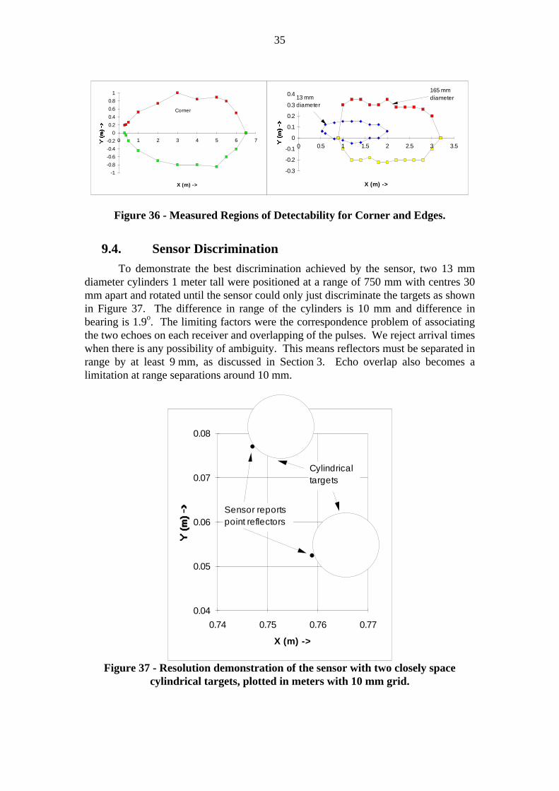
35

X (m) ->

-1

-0.8

-0.6

-0.4

-0.2

0

0.2

0.4

0.6

0.8

1

0 1 2 3 4 5 6 7

Corner

X (m) ->

-0.3

-0.2

-0.1

0

0.1

0.2

0.3

0.4

0 0.5 1 1.5 2 2.5 3 3.5

13 mm diameter

165 mm diameter

Figure 36 - Measured Regions of Detectability for Corner and Edges.

9.4. Sensor Discrimination

To demonstrate the best discrimination achieved by the sensor, two 13 mmdiameter cylinders 1 meter tall were positioned at a range of 750 mm with centres 30mm apart and rotated until the sensor could only just discriminate the targets as shownin Figure 37. The difference in range of the cylinders is 10 mm and difference inbearing is 1.9o. The limiting factors were the correspondence problem of associatingthe two echoes on each receiver and overlapping of the pulses. We reject arrival timeswhen there is any possibility of ambiguity. This means reflectors must be separated inrange by at least 9 mm, as discussed in Section 3. Echo overlap also becomes alimitation at range separations around 10 mm.

X (m) ->

0.04

0.05

0.06

0.07

0.08

0.74 0.75 0.76 0.77

Cylindricaltargets

S ens or reportspoint reflectors

Figure 37 - Resolution demonstration of the sensor with two closely spacecylindrical targets, plotted in meters with 10 mm grid.

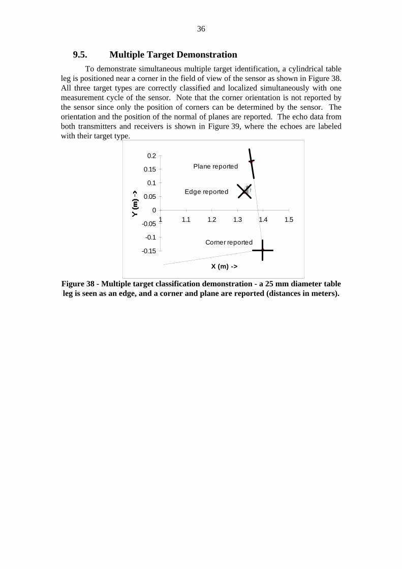
36

9.5. Multiple Target Demonstration

To demonstrate simultaneous multiple target identification, a cylindrical tableleg is positioned near a corner in the field of view of the sensor as shown in Figure 38.All three target types are correctly classified and localized simultaneously with onemeasurement cycle of the sensor. Note that the corner orientation is not reported bythe sensor since only the position of corners can be determined by the sensor. Theorientation and the position of the normal of planes are reported. The echo data fromboth transmitters and receivers is shown in Figure 39, where the echoes are labeledwith their target type.

X (m) ->

-0.15

-0.1

-0.05

0

0.05

0.1

0.15

0.2

1 1.1 1.2 1.3 1.4 1.5



E dge reported

Plane reported

Corner reported

Figure 38 - Multiple target classification demonstration - a 25 mm diameter tableleg is seen as an edge, and a corner and plane are reported (distances in meters).

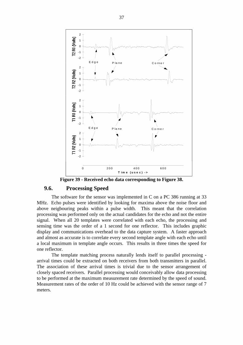
37

-2

-1

0

1

2

-2

-1

0

1

2

-2

-1

0

1

2

-2

-1

0

1

2

T i m e ( u s e c ) ->0 2 0 0 4 0 0 6 0 0

E d g e P la n e C o rn e r

E d g e P la n e C o rn e r

Figure 39 - Received echo data corresponding to Figure 38.

9.6. Processing Speed

The software for the sensor was implemented in C on a PC 386 running at 33MHz. Echo pulses were identified by looking for maxima above the noise floor andabove neigbouring peaks within a pulse width. This meant that the correlationprocessing was performed only on the actual candidates for the echo and not the entiresignal. When all 20 templates were correlated with each echo, the processing andsensing time was the order of a 1 second for one reflector. This includes graphicdisplay and communications overhead to the data capture system. A faster approachand almost as accurate is to correlate every second template angle with each echo untila local maximum in template angle occurs. This results in three times the speed forone reflector.

The template matching process naturally lends itself to parallel processing -arrival times could be extracted on both receivers from both transmitters in parallel.The association of these arrival times is trivial due to the sensor arrangement ofclosely spaced receivers. Parallel processing would conceivably allow data processingto be performed at the maximum measurement rate determined by the speed of sound.Measurement rates of the order of 10 Hz could be achieved with the sensor range of 7meters.

38

10. Conclusions and Future WorkA novel sonar sensor configuration and processing approach has been

presented that can accurately classify and localize planes, corners and edges withoutsensor movement. This has been achieved by adopting physical models fortransmission, propagation, reflectance and reception of ultrasonic pulses combinedwith optimal arrival time processing, all with a reasonable computational burden. Thesensor range and bearing accuracy and target discrimination are often limited only bythe fundamental properties of the transducer, air and reflectors, rather than the sensordata processing.

This paper has shown theoretically that two transmitters and two receivers arenecessary and sufficient for classifying the useful indoor geometric targets of planes,corners and edges. This minimal configuration has been implemented as anexperimental prototype. Range and bearing measurements with errors less than amillimeter and 0.1 degrees have been verified out to 8 meters range. Discriminationof targets separated by as little as 10 mm has been achieved due the narrow pulseshape emitted from the transmitter. Thus the sensor has the capability to workeffectively in cluttered environments.

A template matching approach has been effective in optimally estimating theecho arrival times. Echo shapes for different transmitting and receiving angles andranges are generated and stored. By choosing the best correlation match between theincoming echo and the template set, the optimal arrival time can be estimated. Twoarrival times from the stereo receivers generate a bearing estimate. By transmittingtwo pulses from different transmitters, targets can be classified as planes, corners,edges or unknown. Maximum likelihood estimators for classifying echoes into thesetarget types have been presented in this paper.

A novel feature of the sensor design is the close spacing of the receivers. Thissignificantly reduces the possibility of ambiguity in associating arrival times from thetwo receivers to physical targets. Bearing accuracy is still maintained in practice dueto the optimal arrival time estimation.

The complete received signals are processed by the sensor, as compared tofirst echo systems such as the Polaroid ranging module. This means that distanttargets are not masked by close targets as occurs with the Polaroid ranging module.All targets that return recognizable echoes are reported in our sensor.

Improvements to the sensor are now discussed. The template set can beextended beyond the 20o maximum applied in this paper, for better results at closeranges. The approximation of equal transmitter and receiver angles in the template setcould also be improved by calculating the transmitter angle for each receiver angle inthe template set at close ranges.

Extensions have been presented to allow future three dimensional targetclassification. A useful modification to the sensor is to employ a three dimensionalvector receiver in place of the two dimensional vector receiver presented in the paper.This will allow the rejection of phantom targets due to the pulse propagation not in thehorizontal plane. For example, reflections from the intersection of a floor and wallcould be recognized as not in the horizontal plane of the sensor. The two dimensionalsensor presented here falsely recognizes this reflector as a second plane beyond thewall.

The problem of multiple reflections (apart from single corners) has not beenaddressed in this paper and is a fundamental limitation of all sonar systems. For

39

example, for an edge to be classified and localized incorrectly by the sensor bothtransmitters need to produce the same multiple reflection effect which is unlikely inpractice. Reflectors illuminated by the pulse first bouncing off a plane and back viathe same plane are more easily incorrectly localized. These errors appearindistinguishable to the sensor from real targets at the virtual image location. Theerrors must be rejected by higher level reasoning and different sensor viewpoints thatavoid the intervening plane.

The next stage of research is the incorporation of these sensors into a workingmobile robot for experiments in localization and map building. With the highaccuracy and reliable target classification of the sensors we hope to achieveautonomous robot localization with sonar in unknown indoor environments. Byclassifying targets when sensed, rather than by merging multiple views as with singletransducer systems, the sensor provides significant advantages in associating targetsfor map merging and localization tasks. The high bearing and range accuracy alsoreduces the possibility of incorrect measurement association and of course improvesmap and localization accuracy.

More complex object recognition and docking tasks can be attempted, such asfinding doorways and battery recharging ports. Adaptations of the sensor are alsoenvisaged for obstacle avoidance tasks. For example, a single transmitter and threereceivers could produce range, azimuth and elevation of target without geometricclassification.

Due to our ability to predict accurately the pulse shape as it propagates, it isconceivable that a high repetition pulse rate sonar system could be developed whereincoming pulses can be associated with the firing cycle from their shape andamplitude. Thus pulse rates higher than that dictated by the transmit receive delaymay be then possible.

ReferencesBarshan, B. and Kuc, R. 1990. "Differentiating sonar reflections from corners and

planes by employing an intelligent sensor", IEEE PAMI, Vol 12, No 6, pp 560-569.

Borenstein, J. and Koren, Y. 1988 (April). "Obstacle avoidance with ultrasonicsensors", IEEE Journal Robotics and Automation, , pp 213-218.

Bozma, O. and Kuc, R. 1991. "Characterizing pulses reflected from rough surfacesusing ultrasound", The Journal of the Acoustical Society of America, Vol 89,No 6, pp 2519-2531.

Bozma, O. and Kuc, R. 1991a. "Building a sonar map in a specular environment usinga single mobile sensor" IEEE PAMI Vol 13 No. 12, pp. 1260-1269.

Brown, M. K. 1985 (Dec.). "Feature extraction techniques for recognizing solidobjects with an ultrasonic sensor", IEEE Journal Robotics and Automation, pp.191-205.

Crowley, J. L. 1985 (March). "Navigation for an intelligent mobile robot", IEEEJournal Robotics and Automation, , pp. 31-41.

Elfes, A. 1987. "Sonar-based real world mapping and navigation", IEEE TransRobotics and Automation, pp. 249-265.

Hong, M. L. and Kleeman, L. 1992 (May). "Analysis of ultrasonic differentiation ofthree dimensional corners, edges and planes", IEEE International Conferenceon Robotics and Automation, Nice, France pp 580-584.

40

Iijima, J. and Yuta, S. 1992. "Searching unknown 2-D environment by a mobile robotwith a range sensor", Computers Elect. Engineering Vol 18 No 1 pp 83-98.

Kuc, R. 1988. Introduction to Digital Signal Processing, New York: McGraw-Hill.Kuc, R. 1990 (July). "A spatial sampling criterion for sonar obstacle detection", IEEE

Trans Pattern Analysis and Machine Intelligence, Vol 12, pp. 686-690.Kuc, R. and Siegel, M. W. 1987 (Nov.). "Physically based simulation model for

acoustic sensor robot navigation", IEEE PAMI, Vol 9, No 6, pp 766-778.Larsen, R. J. and Marx, M. L. 1985. An Introduction to Probability and its

Applications, Englewood Cliffs: Prentice-Hall.Leonard, J. F. and Durrant-Whyte, H. F. 1991. "Mobile robot localization by tracking

geometric beacons", IEEE Transactions Robotics and Automation Vol. 7 No 3,pp 376-382.

Manyika, J. M. and Durrant-Whyte, H. F. 1993 (May). "A tracking sonar sensor forvehicle guidance", Proceedings IEEE Robotics and Automation Conference,Atlanta Georgia, pp. 424-429.

McKerrow, P. J. 1993 (Feb.). "Echolocation - from range to outline segments",Proceedings Intelligent Autonomous Systems-3, Pittsburgh, pp. 238-247.

Moravec, H. P. and Elfes, A. 1985. "High resolution maps from wide angle sonar",Proceedings IEEE Robotics and Automation Conference, pp. 116-121.

Munro, W. S. H. et al 1989. "An ultrasonic vehicle guidance system", Proceedings ofIROS 89, Tsukuba Japan, pp.224-227.

Nagashima, Y. and Yuta, S. 1992 (July). "Ultrasonic sensing for a mobile robot torecognize an environment - measuring the normal direction of walls",Proceedings of IROS 92, Raleigh NC, pp. 805-812.

Papoulis, A. 1984. Probability, Random Variables, and Stochastic Processes, 2ndedition New York: McGraw-Hill Book Company.

Peremans, H., Audenaert, K. and Van Campenhout, J. M. 1993. "A high-resolutionsensor based on tri-aural perception", IEEE Trans on Robotics andAutomation, Vol 9, No 1, pp. 36-48.

Polaroid Corporation 1982. Ultrasonic Range Finders.Polaroid Corporation 1987. Data sheet for Series 7000 transducer, Ultrasonic

components group, 119 Windsor St, Cambridge MA 02139 USA..Press, W. H. et al 1990. Numerical Recipes in C, the Art of Scientific Computing,

Cambridge NY: Cambridge Uni Press.Sabatini, A. 1992. "Active hearing for external imaging based on an ultrasonic

transducer array", Proceedings of IROS 92, Raleigh, pp. 829-836.Sasaki, K. and Takano, M. 1992. "Classification of object's surface by acoustic

transfer function", Proceedings of IROS 92, Raleigh, pp 821-828.Suoranta, R. 1992 (Oct.). "Novel ultrasonic beamforming method based on nonlinear

filtering", 1992 IEEE Ultrasonic Symposium, Tucson, Arizona.Weast, R. C. and Astle, M. J. (Editors) 1978. CRC Handbook of Chemistry and

Physics, 59th edition, Boca Raton, Florida: CRC Press.Whalen, A. D. 1971. Detection of Signals in Noise, Orlando: Academic Press Inc.Woodward, P. M. 1964. Probability and Information Theory with Applications to

Radar, 2nd edition, Oxford: Pergamon Press.Yang, M., Hill, S. L. and Gray, J. O. 1992. "Design of ultrasonic linear array system

for multi-object identification", Proceedings of IROS 92, Raleigh, pp. 1625-1632.

mobile robot sonar for target localization and...

Documents