mobile payment adoption: an empirical investigation on alipay
TRANSCRIPT

Mobile Payment Adoption:An Empirical Investigation on Alipay
Yuqian XuGies College of Business, University of Illinois at Urbana-Champaign, Champaign, IL 61820, [email protected]
Anindya GhoseStern Business School, New York University, New York, NY 10012, [email protected]
Binqing XiaoIndustrial Engineering Department, Nanjing University, China, 210093, [email protected]
The rapid development of mobile technology has introduced a new channel for consumer consumption, in
addition to traditional online PC and offline (physical card) payment channels. In this paper, we investigate
the determinants and outcomes of mobile channel adoption on consumer consumption behaviors. We utilize a
unique data set from one of the largest banks in China, which contains the consumer credit card consumption
from PC, offline, and mobile payment channels. The mobile payment channel under study here is from
Alipay, which is now the world’s largest mobile payment platform. In our work, we find that both higher
service demand and higher local penetration are associated with earlier mobile channel adoption. For the
post-adoption behavior analysis, we show that the total transaction amount increases by around 2.4% after
the Alipay adoption, and the total transaction frequency increases by around 23.5%. The relationship is even
stronger for medium income consumers. Furthermore, we find that Alipay channel acts as a substitute for the
offline channel, and as a complement for the PC payment channel. Both substitution and complementarity
effects increase over time. Finally, we find that the increased credit card transaction activity and profitability
are likely to be driven by hedonic shopping behavior with low value items. Our work aims to bring managerial
implications for bank and retail managers on multi-channel management.
Key words : Alipay, adoption, mobile payment, channel, PC, offline, online, credit card.
1
Electronic copy available at: https://ssrn.com/abstract=3270523

Author:2 Article submitted to Management Science; manuscript no.
1. INTRODUCTION
With the rapid development of smartphones, mobile payment is becoming more and more
popular among consumers and is gradually changing the non-cash commerce around the
world. According to the Federal Reserve’s study,1 the amount of mobile transaction in
the US reached 1.3 billion in 2015, accounting for 5.6% of the total non-cash payment
transactions. In some countries, such as China, mobile payment has already become a
counterpart of bank cards. According to the People’s Bank of China,2 mobile transactions
have surpassed total transactions made by physical bank cards by 43%. In addition to the
amount of transactions, the number of different mobile payment users is also increasing
rapidly. For instance, PayPal currently has around 200 million users who have spent US$282
billion in 25 currencies in 202 countries (Farnon (2016)). Also, Apply Pay now has over
87 million users around the world, with more than US$1 million in retail consumption
covering major markets, such as the US, Canada, the UK, Italy, France, New Zealand,
Australia, Russia, and China (see Statista (2017)). Furthermore, according to Bloomberg,3
Apple Pay is adding 1 million new consumers per week. The mobile payment channel under
study in this paper is Alipay, which is now the largest mobile payment platform in the
world4. On December 23, 2010, Alipay collaborated with Bank of China to start a new
service called “fast payment of credit card,”5 which simplified the payment process. After
the establishment of this innovative service, Alipay officially began its mobile payment
1 https://www.federalreserve.gov/newsevents/pressreleases/files/2016-payments-study-recent-developments-
20170630.pdf
2 http://www.pbc.gov.cn/goutongjiaoliu/113456/113469/3273108/2017031514423288068.pdf
3 https://www.bloomberg.com/quicktake/mobile-payments
4 John Heggestuen (11 February 2014). Alipay Overtakes PayPal As The Largest Mobile Payments Platform In The
World. Business Insider. wiki
5 http://it.sohu.com/20101223/n278474761.shtml
Electronic copy available at: https://ssrn.com/abstract=3270523

Author:Article submitted to Management Science; manuscript no. 3
services. As of 2013, Alipay has overtaken PayPal as the largest mobile payment platform
in the world. During the fourth quarter of 2016, Alipay had a 54% market share of China’s
US$5.5 trillion mobile payment market.6 Because mobile payment has become a new trend
for consumer consumption, firms and banks must understand its economic impact.
So far as we know, limited prior work has looked into the new mobile payment channel
adoption and the intrinsic interdependencies that are related to mobile, PC, and offline
(physical card) payment channels. Therefore, our work aims to take an initial step in
understanding the determinants and outcomes of mobile payment adoption. Our ultimate
goal is then to bring managerial implications for bank and retail managers on multi-channel
management. To do so, we utilize a unique data set from one of the largest banks in China,
which contains the consumer credit card transactions from PC, offline, and mobile payment
(Alipay) channels. Our focal bank is the first bank in China that collaborated with Alipay,
and the collaboration started in December 2010. This data set recorded the transactions
of 4,541,583 credit cards issued between 1989 and 2013 from 3,182,237 consumers. Our
observed transactions were made between September 2010 and February 2013. With our
data set, we are able to identify the specific date each consumer first used Alipay to conduct
transactions. We can then exploit the variation among users’ Alipay adoption dates, and
use our econometric methods to estimate the changes in consumption from the PC channel
and physical credit card channel before and after the Alipay adoption.
In the pre-adoption analysis, we conduct survival analysis and find that higher service
demand is associated with earlier mobile channel adoption; and the relationship is even
stronger for frequent travelers due to channel ubiquity. More specifically, we find that a
consumer’s time to adopt the mobile payment channel is reduced by around 0.5% with
6 https://www.ft.com/content/e3477778-2969-11e7-bc4b-5528796fe35c
Electronic copy available at: https://ssrn.com/abstract=3270523

Author:4 Article submitted to Management Science; manuscript no.
a one-unit increase in transaction frequency of the month before adoption. Furthermore,
we find that if a consumer is a frequent traveler, his time to adopt the mobile payment
channel is reduced by at least 0.79% with a one-unit increase in transaction frequency of
the month before adoption. Finally, higher local penetration is also associated with earlier
mobile channel adoption, and a consumer’s time to adopt the mobile payment channel is
reduced by around 0.3% with a one-unit increase in local penetration level.
In the post-adoption analysis, we employ the difference-in-differences (DID) methodology
coupled with propensity score matching (PSM) to estimate our main results. Controlling
for the service demand and local penetration for matched treatment and control groups,
we find that the total transaction amount increases by around 2.4% after Alipay adoption,
and the total transaction frequency increases by around 23.5%. Therefore, mobile channel
adoption is associated with increased credit card transaction activity and profitability, and
we further find that the relationship is increasing over time and is even stronger for medium
income consumers. We also find that the mobile payment channel acts as a substitute
for the offline (physical card) channel and as a complement for the PC payment channel.
More specifically, for the PC payment channel, the total transaction amount increases
by around 0.3% after the Alipay adoption, the share of the transaction amount increases
by around 0.01%, the total transaction frequency increases by around 0.18%, and the
share of transaction frequency increases by around 0.016%. On the other hand, for the
physical card channel, the total transaction amount decreases by around 3.9% after the
Alipay adoption, the share of the transaction amount decreases by around 26.2%, the total
transaction frequency decreases by around 9.4%, and the share of transaction frequency
decreases by around 39.8%. Moreover, we find both substitution and complementarity
effects increase over time. Finally, we find that the increased credit card transaction activity
Electronic copy available at: https://ssrn.com/abstract=3270523

Author:Article submitted to Management Science; manuscript no. 5
and profitability are likely to be driven by hedonic shopping behavior with low value items.
In particular, mobile channel adoption has the largest effect on the groceries category,
followed by entertainment, travel, and service categories.
The remainder of the paper is organized as follows. Section 2 provides a literature review.
Section 3 discusses our main hypotheses. Section 4 presents the details of our data sources.
Section 5 describes our econometric model. Section 6 discusses our empirical results for
both pre- and post-adoption, subset analysis, and robustness checks. Section 7 summarizes
our results and outlines future research directions.
2. RELATED LITERATURE
In this section, we review three streams of literature that are closely related to our work,
namely, (i) PC channel adoption, (ii) features of mobile phone channel, and (iii) interde-
pendencies among different channels.
The first stream of work closely related to ours is on the adoption of the PC channel,
which is found to be associated with changes in service consumption, cost to serve, and
consumer profitability (see Hitt and Frei (2002) and Campbell and Frei (2010)). In par-
ticular, consumers who adopt PC channel are found to be more profitable although the
adoption will cause a reduction in short-term consumer profitability (Campbell and Frei
(2010)); moreover, consumers who adopt PC channel have a lower propensity to leave the
bank (Xue et al. (2011)). Recent work has started looking into the adoption of mobile
banking channel, and find that the mobile banking channel serves as a complement to
the PC banking channel (Liu et al. (2017)). However, so far limited work has been done
on exploring the adoption of mobile payment channel and the associated consequences
of mobile payment adoption. In this paper, we want to fill this void by investigating the
determinants and outcomes of mobile payment channel adoption on consumer consumption
behaviors.
Electronic copy available at: https://ssrn.com/abstract=3270523

Author:6 Article submitted to Management Science; manuscript no.
The second stream of literature closely related to our work is on the features of mobile
phone consumption. Prior work has looked into the effect of the screen size when analyzing
the impact of mobile phone on consumption decisions (see Chae and Kim (2004), Kim
et al. (2011), and Ghose et al. (2012)). Recent research has also focused on improving the
consumer experience of browsing the web on their smartphones (Adipat et al. (2011)).
Portability is also a key feature of mobile phones. Although PCs enable consumers to hold
a global perspective when shopping via the computer (Overby and Lee (2006)), the restric-
tion of portability offsets this benefit. Universality, as another essential feature, refers to
a channel’s ability to provide universal and stable service in space and time. Compared
to PCs, mobile channels overcome the constraints of places, which constantly support
consumers in activities such as information access or immediate transactions (Jung et al.
(2014)). However, the storage limitation of mobile devices constrains the volume of infor-
mation access and impairs the quality of PC services (Napoli and Obar (2014)). Thus,
determining the moderating features associated with mobile channel adoption is crucial
for bank and retail managers.
The third stream is the interdependencies among different channels, which has been
studied by a significant number of papers in the past few years. In general, findings in
these papers provide significant managerial insights into firms’ investment-strategies prob-
lem of whether to diversify their investments or concentrate on a single retail channel.
These papers have looked into the following problems: (1) the effects of substitution and
complementarity between PC and offline channels, (i.e., Brynjolfsson et al. (2009), Choi
et al. (2008), Ellison and Ellison (2006), Forman et al. (2009), Goolsbee (2001), and Prince
(2007)); (2) how offline sales channels could be affected by mobile ads based on location
or context (see Hui et al. (2013) and Molitor et al. (2016)); and (3) the interdependencies
Electronic copy available at: https://ssrn.com/abstract=3270523

Author:Article submitted to Management Science; manuscript no. 7
between the mobile and PC channels (see Bang et al. (2013) and Ghose and Han (2011)).
From these papers, we can see that a new channel will probably be established under the
condition that it has the ability to provide consumers with extra utility relative to what
they have received from the previous channels. For example, when the offline stores enter
the market, local consumers will shift away significantly from the previous PC channels
(Forman et al. (2009)). Despite the benefits of PC shopping, such as lower prices and a
wider area of product selection, the potential reasons why consumers turn to their local
offline stores may include lower traveling and shipping costs, as well as the ability to check
quality. Moreover, PC and offline channels can complement each other (Luo et al. (2013)),
and mobile and PC channels can substitute for and complement each other simultaneously,
depending on the product category (Bang et al. (2013)). Finally, the tablet channel acts
as a substitute for the PC channel and a complement for the smartphone channel (Xu
et al. (2016)). However, so far as we know, limited work has looked into the new mobile
payment channel and the intrinsic interdependencies that are related to mobile, PC, and
offline (physical card) payment channels. Thus, another goal of this paper is to explore
interdependencies among the three channels.
3. HYPOTHESES
A new channel will probably be established under the condition that it has the ability
to provide consumers with extra utility relative to what they have received from the pre-
vious channels. Random utility theory (McFadden (1974)) shows that consumers adopt
the product that provides them with the highest utility given the costs and benefits of
the product, and idiosyncratic consumer tastes. In our work, a consumer’s direct cost and
benefit are captured by the factor of service demand and the indirect cost and benefit are
mainly captured by the factor of local penetration. We discuss how these two factors are
Electronic copy available at: https://ssrn.com/abstract=3270523

Author:8 Article submitted to Management Science; manuscript no.
associated with consumer mobile channel adoption in Section 3.1. After the mobile channel
adoption, the usage of this new channel may change consumers consumption behaviors.
We analyze the consumer behavior changes from three perspectives, namely transaction
activities, consumer profitability, and channel substitution and complementarity. We study
these three aspects in details in Section 3.2.
3.1. Hypotheses: Mobile Channel Adoption
In this subsection, we discuss our two main hypotheses on pre-adoption behavior. We
consider two driven factors, namely service demand and local penetration.
Service Demand. Previous research on Internet payment adoption has shown that con-
sumers whose service-interaction demand is high would gain greater overall benefits from
any kind of service innovation, and thus they are more likely to adopt Internet payment
(see Lee and Lee (2001) and Xue et al. (2011)). Similarly, here those consumers who have
high service demand would also be more likely to adopt mobile payment. In our analysis,
following Xue et al. (2011), we use the transaction frequency to measure the consumers’
service demand. Moreover, previous work has shown that compared to PCs, mobile chan-
nels overcome the constraints of places due to channel ubiquity, and constantly support
consumers in activities such as information access or immediate transactions (Jung et al.
(2014)). This characteristic of channel ubiquity also enables users to enjoy videos to pass
the time and mitigate solitude when traveling (O’Hara et al. (2007)). Bang et al. (2013)
show that ubiquity is an important feature that measures the channel capability. In our
context, similar to Xu et al. (2016), we consider channel ubiquity as the channel’s abil-
ity to offer instant Internet access wherever and whenever a user wants. Intuitively, the
PC channel is constrained by Internet usage and hardware. However, the mobile channel
overcomes this limitation by offering ubiquitous Internet access (see Jung et al. (2014)
Electronic copy available at: https://ssrn.com/abstract=3270523

Author:Article submitted to Management Science; manuscript no. 9
and Venkatesh et al. (2003)). Therefore, we expect that the relationship between service
demand and earlier mobile channel adoption is stronger for consumers in need of channel
ubiquity, i.e., frequent travelers. We now summarize our first hypothesis as follows.
Hypothesis 1 (H1). Higher service demand is associated with earlier mobile channel
adoption; and the relationship is even stronger for frequent travelers due to channel ubiq-
uity.
Local Penetration. Previous product diffusion and network effects literature has shown
that the number of compatible products adopters may affect the product demand, see Bass
(1969) and Katz and Shapiro (1985). Moreover, the Internet payment adoption literature
has shown that local penetration is positively related to faster Internet payment adoption
(Xue et al. (2011)). In the mobile payment context, although consumers may not directly
interact with each other, following similar two reasons as Xue et al. (2011), we expect local
penetration plays an important role in mobile payment adoption. The first reason is the
local word-of-mouth effects found in may previous literature for other products such as PC
groceries, see Stavins (2001), Goolsbee and Klenow (2002), Forman et al. (2008), Choi et al.
(2010). The second reason is the indirect effects such as complementary investments made
by service providers who interact with mobile payment channel and want to expand service
payment channels, see Xue et al. (2011). Both explanations suggest that one may adopt
mobile payment channel faster with more prior adopters in a close area. In our analysis, we
use the number of existing Alipay adopters within the same zip code area as the adopter
under study to measure the level of local penetration. We specify our hypothesis as follows.
Hypothesis 2 (H2). Higher local penetration is associated with earlier mobile channel
adoption.
Electronic copy available at: https://ssrn.com/abstract=3270523
Author:10 Article submitted to Management Science; manuscript no.
3.2. Hypotheses: Post-adoption Behavior Changes
In this subsection, we discuss our three main hypotheses on post-adoption behavior. We
consider three outcomes, i.e., transaction activities, consumer profitability, and channel
substitution and complementarity.
Transaction Activities. One key advantage of mobile channel is the convenience of car-
rying. Compared to mobile phones, devices with larger screens have a negative affect on
the convenience of carrying and on usage rates (Kim et al. (2011)). Similarly, although
PCs enable consumers to hold a global perspective when shopping via the PC (Overby
and Lee (2006)), the restriction of portability offsets this benefit. Therefore, facing the key
advantage of convenience, mobile channel adopters are likely to increase the number of
transactions they perform. Furthermore, we expect transaction activities to be different
across different product values and consumers. For example, low-value products, such as
groceries, are generally more likely to be hedonic shopping targets and e-channel appears
more attractive to small buyers (Langer et al. (2012)); therefore mobile channel adopters
might be more likely to purchase low value products. We next specify our hypothesis on
transaction activity as follows.
Hypothesis 3 (H3). Mobile channel adoption is associated with increased credit card
transaction activity, especially for low-value items.
Consumer Profitability. On one hand, the introduction of mobile payment channel makes
consumption much easier, and increased transaction activities are likely to lead to greater
consumer profitability. Prior research has shown that the online banking adoption is associ-
ated with increasing consumer profitability (Xue et al. (2011)), and multichannel customers
are more profitable than they would be if they were not multichannel (Montaguti et al.
(2016)). However, on the other hand, if most increased activities are associated with lower
Electronic copy available at: https://ssrn.com/abstract=3270523
Author:Article submitted to Management Science; manuscript no. 11
value items, then the overall profitability of consumer is not necessarily increasing. Fol-
lowing Xue et al. (2011), we use the monthly transaction amount to measure consumer
profitability, and we thus test the following hypothesis.
Hypothesis 4 (H4). Mobile channel adoption is associated with increased credit card
consumer profitability.
Channel Substitution and Complementarity. Prior research has shown that mobile and
PC channels can substitute for and complement each other simultaneously, depending on
the product category (Bang et al. (2013)), and the tablet channel acts as a substitute for
the PC channel and a complement for the smartphone channel (Xu et al. (2016)). Recent
work also finds that the mobile banking channel serves as a complement to the PC channel
(Liu et al. (2017)). In the next hypothesis, we want to explore the impact of the mobile
payment channel on consumer consumption, and find the intrinsic interdependencies that
are related to mobile, PC, and offline payment channels. We test the following hypothesis.
Hypothesis 5 (H5). Mobile channel serves as substitute of physical card channel; but
as complement of PC channel.
4. DATA
Our credit card data set contains three parts. The first part records 2,016,132 credit card
issuances between 1989 and 2013 from one of the largest banks in China7 to consumers
in Jiangsu Province. This issuance data discloses detailed information on the card-issuing
date, type of card, annual fee, credit limit, and so on. Here, by knowing the credit card
issuance date, we can easily compute the length of the usage of each credit card, which
later we use as an important control variable in our model.
7 Note that the first credit card in China was issued on February 1, 1987.
Electronic copy available at: https://ssrn.com/abstract=3270523
Author:12 Article submitted to Management Science; manuscript no.
The second part of our data set contains 1,541,769 consumers’ demographic informa-
tion, for example, age, gender, job position (manager or not), education (graduate degree,
bachelor’s degree, high school degree, middle high school degree, elementary school degree,
and non-educated), marriage status (married or not), living status (rent or own), and so
on.
The third part discloses the consumer transaction-level information from September
2010 to February 2013 (29 months), including transaction amount, account balances, trans-
action date, type of transaction (education, service, healthcare, entertainment, groceries,
and travel), interest rate, reward points, and so on. In this part of our data set, we have
159,954,104 observations. By knowing the transaction dates, we can later easily compute
the number of transactions (frequency) per month. Moreover, for each transaction obser-
vation, we can observe an associated label indicating the payment channel, i.e., online PC,
Alipay (mobile channel), offline, etc.8 Note that the payment here for each transaction is
still made through credit card, and each credit card is used through one of the three (online
PC, Alipay, and offline) channels. If the payment channel of one transaction is labeled as
Alipay, then it means that the credit card used for this transaction is linked to Alipay, and
when a consumer makes a payment, he can scan mobile phone codes in restaurants or stores
instead of using a physical card. Note that Alipay also allows consumers to make payments
or transfers to their friends and relatives (as in Paypal), however our study only focuses on
commercial transactions and does not include transactions made to any individual person.
Table 1 shows the summary statistics of key variables in our data set.
8 Note that during our observation period between September 2010 and February 2013, Alipay is the only dominating
mobile payment app in China. The second largest mobile payment app, WeChat Pay, was launched in September
2014.
Electronic copy available at: https://ssrn.com/abstract=3270523

Author:Article submitted to Management Science; manuscript no. 13
Table 1 Summary Statistics
Variable Definition Mean Sd. Min Max N
Numerical Variables
CDT LMT Credit limit in RMB 12,878 52,766 0 5,000,000 4,541,583CDT LEN Card usage length in months 25 14 0 192 4,541,583CDT TYP Main (1) or attached (0) card 0.9700 0.1700 0 1.000000 4,500,933GENDER Male (1) or female (0) 0.4600 0.5000 0 1.000000 3,181,418AGE Age of card holder 29 5.7 12 93 3,181,418TXN AMT Transaction amount per month in RMB 2,239.4 2,133.8 0 4,986,592 159,954,104TXN AMT 5 Average transaction amount last 5 months in RMB 2,478.3 2,259.6 0 4,295,375 159,954,104TXN CNT Transaction frequency per month 72.1 69.8 0 1,500.00 28,619,173ANU FEE Annual fee in RMB 3.2100 56.300 0 3,600.000 28,634,369CDT BAL Account credit balances 4,520.2 23,742 0 2,000,000 335,395
Binary Variables
JOB POS Manager (1) or not (0) 0.35 0.13 0 1 3,179,303EDU0 Non-educated (1) or not (0) 0.11 0.05 0 1 2,381,090EDU1 Elementary school (1) or not (0) 0.15 0.06 0 1 2,381,090EDU2 Middle high school (1) or not (0) 0.16 0.10 0 1 2,381,090EDU3 High school (1) or not (0) 0.15 0.06 0 1 2,381,090EDU4 Bachelor (1) or not (0) 0.27 0.17 0 1 2,381,090EDU5 Graduate (1) or not (0) 0.10 0.05 0 1 2,381,090MAR STS Married (1) or not (0) 0.48 0.27 0 1 2,788,549LIV STS Own (1) or rent (0) 0.44 0.23 0 1 3,154,055
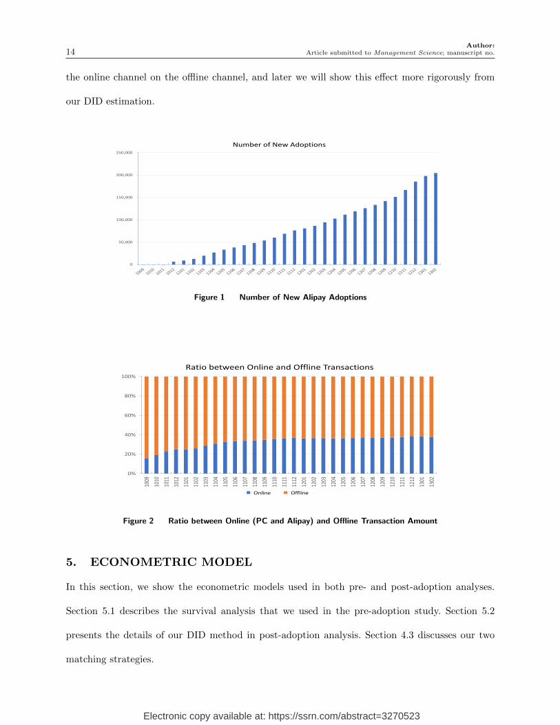
Next, we describe some initial analysis of our data set. First, we find that around 35.14% of
the consumers in the data set have used online payment methods, including both PC and mobile
channels. Among the online channels, Alipay has 204,547 users, and the PC channel has 244,981
users during our entire observation period. Therefore, we can see that by the end of February 2013,
Alipay had almost as many users as the traditional PC payment channel.
Figure 1 shows the number of new consumers who adopted Alipay each month during our
observation period. We can see that, starting from December 2010, when our focal bank started
to collaborate with Alipay, the number of accumulated new adoptions has been growing steadily.
In February 2013, the number of new adoptions had grown to 204,547 (13.3%), which shows that
mobile payment has become more and more popular. Figure 2 compares the percentage of the online
transaction (including both mobile and PC channels) amount with the percentage of the offline
transaction amount made in each month. We can see that the fraction of the online transaction
amount has grown steadily over time, especially since October 2010, whereas the offline transaction
amount has decreased gradually. Figure 2 shows the initial analysis on the substitution effect of
Electronic copy available at: https://ssrn.com/abstract=3270523
Author:14 Article submitted to Management Science; manuscript no.
the online channel on the offline channel, and later we will show this effect more rigorously from
our DID estimation.
0
50,000
100,000
150,000
200,000
250,000
Number of New Adoptions
Figure 1 Number of New Alipay Adoptions
0%
20%
40%
60%
80%
100%
1009
1010
1011
1012
1101
1102
1103
1104
1105
1106
1107
1108
1109
1110
1111
1112
1201
1202
1203
1204
1205
1206
1207
1208
1209
1210
1211
1212
1301
1302
Ratio between Online and Offline Transactions
线上交易 线下交易Online Offline
Figure 2 Ratio between Online (PC and Alipay) and Offline Transaction Amount
5. ECONOMETRIC MODEL
In this section, we show the econometric models used in both pre- and post-adoption analyses.
Section 5.1 describes the survival analysis that we used in the pre-adoption study. Section 5.2
presents the details of our DID method in post-adoption analysis. Section 4.3 discusses our two
matching strategies.
Electronic copy available at: https://ssrn.com/abstract=3270523
Author:Article submitted to Management Science; manuscript no. 15
5.1. Mobile Channel Adoption Analysis
To understand the determinants of mobile payment adoption, we conduct survival analysis, where
a subject leaves the panel when the adoption event happens. Therefore, this approach links the
explanatory variables with the time when consumers adopt the mobile payment channel. Note that
a number of approaches can be used for survival analysis, for instance, the accelerated failure time
(AFT) and proportional hazard (PH) models. Following Tellis et al. (2003) and Xue et al. (2011),
we use a log-logistic distribution AFT model, and consider both the regular regression coefficients
in the log-time format and the time-ratio coefficient, which is computed as the ratio of fail time to
normal time. Note that parametric models have been shown to be more statistically efficient than
nonparametric or semi-parametric models in settings where the focus is on the effects of covariates
that evolve over time.
We now specify our log-logistic distribution AFT model. Denote ti as the event time of adoption
for consumer i, xi as a set of covariates, and εi as the error term. We then have the following
regression function:
ln(ti) = xiβx + εi, (1)
where βx is the set of parameter weights to be estimated. Here, if a regular coefficient is negative
or a time ratio coefficient is less than 1, the result implies faster adoption.
To test our two hypotheses on service demand and local penetration, we now define the key
measures. We first define two measures to compute service demand. The first measure (denoted as
M1) is the same as Xue et al. (2011), which computes each consumer’s total transaction frequency
in the month prior to adoption. As a robustness check, we compute a second measure (denoted
as M2) that is the monthly average transaction frequency before adoption. Next, to define the
frequent and infrequent travelers, we compute the percentage of transactions made in cities other
than the focal consumer’s residential city. We then compute the sample average of this percentage
(0.16 on average). Consumers with values above the sample average are defined as frequent traveler,
Electronic copy available at: https://ssrn.com/abstract=3270523

Author:16 Article submitted to Management Science; manuscript no.
and the ones below the sample average are defined as infrequent traveler. Finally, to discuss the
impact of local penetration on mobile channel adoption, we use the number of existing Alipay
adopters within the same zip code area as the adopter under study to measure the level of local
penetration.
5.2. Post-Adoption Analysis: Difference-in-Difference
Following the same approach as Xu et al. (2016), we use DID together with matching to account
for unobserved systemic bias. The DID technique is an econometric method traditionally used to
measure the treatment effect in a given time period through measuring the difference between a
group that received the treatment and a control group that did not (see Meyer (1995)). In our
work, the treatment group consists of consumers who use Alipay, and the control group consists of
consumers who did not use Alipay during our observation time period. By obtaining the first time
the treated group of consumers use Alipay after our focal bank’s collaboration with Alipay, our DID
approach is able to measure the average treatment effect over the treated group. In particular, we
measure the impact of the introduction of the mobile payment channel on the overall transaction
frequency and amount, as well as the impact on PC payment and offline channels. The central
assumption of DID is the parallel trends, i.e., the trends in the outcome variable would have been
parallel in the treated and control groups if there had been no treatment. We indeed find the trends
to be parallel before the intervention. Note that it is not necessary to have random assignment for
the parallel trends assumption to hold, however the assumption might fail if assignment was based
on some characteristics of the groups. To further account for potential endogenous assignment bias,
we later conduct the synthetic control groups method (see Abadie and Gardeazabal (2003), Abadie
et al. (2010), Abadie et al. (2015)) in Section 6.4, and find our results remain consistent.
To make the treatment and control groups comparable, we further adopt matching strategies,
which we will discuss in Section 5.3, to derive a sample of treated consumers with similar observed
characteristics with a sample of untreated consumers. The idea of our matching strategies is that
each Alipay user is paired with a similar non-user in terms of the propensity of being treated. This
Electronic copy available at: https://ssrn.com/abstract=3270523
Author:Article submitted to Management Science; manuscript no. 17
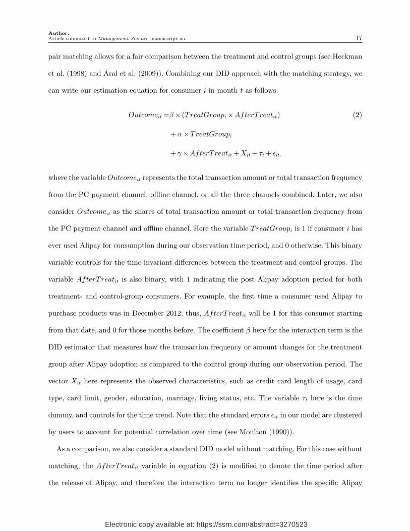
pair matching allows for a fair comparison between the treatment and control groups (see Heckman
et al. (1998) and Aral et al. (2009)). Combining our DID approach with the matching strategy, we
can write our estimation equation for consumer i in month t as follows:
Outcomeit =β× (TreatGroupi×AfterTreatit) (2)
+α×TreatGroupi
+ γ×AfterTreatit +Xit + τt + εit,
where the variableOutcomeit represents the total transaction amount or total transaction frequency
from the PC payment channel, offline channel, or all the three channels combined. Later, we also
consider Outcomeit as the shares of total transaction amount or total transaction frequency from
the PC payment channel and offline channel. Here the variable TreatGroupi is 1 if consumer i has
ever used Alipay for consumption during our observation time period, and 0 otherwise. This binary
variable controls for the time-invariant differences between the treatment and control groups. The
variable AfterTreatit is also binary, with 1 indicating the post Alipay adoption period for both
treatment- and control-group consumers. For example, the first time a consumer used Alipay to
purchase products was in December 2012; thus, AfterTreatit will be 1 for this consumer starting
from that date, and 0 for those months before. The coefficient β here for the interaction term is the
DID estimator that measures how the transaction frequency or amount changes for the treatment
group after Alipay adoption as compared to the control group during our observation period. The
vector Xit here represents the observed characteristics, such as credit card length of usage, card
type, card limit, gender, education, marriage, living status, etc. The variable τt here is the time
dummy, and controls for the time trend. Note that the standard errors εit in our model are clustered
by users to account for potential correlation over time (see Moulton (1990)).
As a comparison, we also consider a standard DID model without matching. For this case without
matching, the AfterTreatit variable in equation (2) is modified to denote the time period after
the release of Alipay, and therefore the interaction term no longer identifies the specific Alipay
Electronic copy available at: https://ssrn.com/abstract=3270523
Author:18 Article submitted to Management Science; manuscript no.
adoption date for each user, but rather a generic date that affects the entire group of potential
adopters through the release of Alipay. The coefficient β then estimates an average treatment effect
of Alipay adoption.
5.3. Post-Adoption Analysis: Matching
We now discuss our two main matching strategies, namely, static and dynamic matching. In static
matching, treated users are matched with non-adopters who resemble them most closely in terms
of their overall propensity scores. Under static matching, the matched control users remain the
same for the entire study period; while dynamic matching requires unique propensity scores for
Alipay adopters for each time unit, and hence adopters are matched with different non-adopters
over time. Following Xu et al. (2016), we here use one month as each time unit. Given the fact that
some attributes of users change over time, the dynamic matching procedure is likely to perform
better, because it accounts for time-varying factors.
To compute the propensity scores for both strategies, we consider covariates such as age, gender,
education, marriage, living status, total transaction amount in the past five months, credit limit,
account balances, local penetration and so on, because these factors are likely to affect Alipay adop-
tion and spending behaviors, see Table 2. In particular, to account for the impact of service demand
and local penetration on adoption decision, we include these two variables as our covariates in the
matching process. We utilize the same set of covariates across all matching procedures. We then
adopt different matching algorithms to assess the robustness of the results with respect to different
matched samples within two types of matching procedures. We first conduct our baseline matching,
that is, to utilize one-to-one matching with replacement to derive the closest matched non-adopter.
Under this process, almost all Alipay adopters (92.1%) have been appropriately matched. Next, we
conduct one-to-one matching without replacement to assess whether the inclusion of more control
users would affect the results. Third, we use nearest-three-neighbors matching as another robust-
ness check. Finally, we conduct matching specifications using the common support requirement
and a tighter caliper size to further assess the stability of results under more stringent matching
conditions.
Electronic copy available at: https://ssrn.com/abstract=3270523

Author:Article submitted to Management Science; manuscript no. 19
To evaluate our matching results, we compare the propensity score distributions of the matched
and unmatched samples (Caliendo and Kopeinig (2008); Haviland A. (2007)), as shown in Figures
3 and 4. In general, we find the distributions for control and treated users to be more similar after
matching. We also conduct a Kolmogorov-Smirnov test to compare the distributions, and find a
strong match between the treated and matched control users.
Following Haviland A. (2007), we next compare the standardized bias before and after matching.
We first compute the standardized bias before matching as:
SBbefore = |µxt −µxp |/√
0.5× (s2xt + s2xp), (3)
where µxt and s2xt are the mean and variance of covariate X for the treated group consumers before
matching, and µxp and s2xp are the mean and variance for unmatched control group consumers. We
next calculate the standardized bias after matching as follows:
SBafter = |µxt −µxc |/√
0.5× (s2xt + s2xc), (4)
where µxt and s2xt are the mean and variance of covariate X for the treated group consumers after
matching, and µxp and s2xp are the mean and variance for the matched control group consumers.
We present the results for the standard bias and the percentage improvement of matching in the
following Table 2.
From Table 2, we can see that before matching, the covariates related to purchase behavior
via Alipay are quite unbalanced. The biases between the treated and control groups are greatly
reduced across most covariates after matching. We further conduct t-test to compare the means
of the treatment and control groups after matching, and the results confirm that the means are
statistically similar after matching.
Electronic copy available at: https://ssrn.com/abstract=3270523

Author:20 Article submitted to Management Science; manuscript no.
1.5
1.0
0.5
00.1 0.2 0.3 0.4 0.5 0.6 0.7 0.8 0.9 1.0
Matched Control Group
Treatment Group
Unmatched Control Group
Figure 3 Estimated Propensity Score for Static Matching
1.5
1.0
0.5
00.1 0.2 0.3 0.4 0.5 0.6 0.7 0.8 0.9 1.0
Matched Control Group
Treatment Group
Unmatched Control Group
Figure 4 Estimated Propensity Score for Dynamic Matching
Electronic copy available at: https://ssrn.com/abstract=3270523

Author:Article submitted to Management Science; manuscript no. 21
Table 2 Comparison before and after Matching
Std. Bias (Before) Std. Bias (After) % Improvement
Static Matchinglog(TXN AMT) 0.1347 0.0004 99.74log(TXN CNT) 0.9707 0.7188 25.95GEN 0.2661 0.2420 9.07 bEDU0 0.3517 0.2343 33.37EDU1 0.0422 0.0474 -12.31EDU2 0.2819 0.2731 31.32EDU3 0.1462 0.0820 43.92EDU4 0.1427 0.1474 -3.29EDU5 0.0065 0.0071 -8.17MAR STS 0.0418 0.0442 -5.69CDT LEN 0.0022 0.0022 1.74CDT TYP 0.0006 0.000006 99.01NUM CDT 0.3179 0.3220 -1.28CDT LMT 0.0024 0.0003 87.50LIV STS 0.4030 0.3523 12.56JOB POS 0.0892 0.0053 94.05AGE 0.0776 0.0069 91.11TXN AMT 5 0.1380 0.0699 49.35CDT BAL 0.0685 0.0099 85.55ANU FEE 0.0377 0.0084 77.72PENETRATION 0.0135 0.0079 41.48
Dynamic Matchinglog(TXN AMT) 0.1347 0.0026 98.07log(TXN CNT) 0.9708 0.7119 26.66GEN 0.2661 0.2770 -4.09EDU0 0.3517 0.3037 13.66EDU1 0.0422 0.0371 12.13EDU2 0.2819 0.2728 3.61EDU3 0.1462 0.1254 14.24EDU4 0.1427 0.1594 -11.66EDU5 0.0066 0.0074 -13.42MAR STS 0.0418 0.0506 -21.07CDT LEN 0.0022 0.0021 2.66CDT TYP 0.0006 0.0001 83.33NUM CDT 0.3179 0.2762 13.11CDT LMT 0.0024 0.0024 -0.95LIV STS 0.4030 0.4171 -3.51JOB POS 0.0892 0.0100 88.73AGE 0.0776 0.0052 93.30TXN AMT 5 0.1380 0.0511 62.97CDT BAL 0.0685 0.0094 86.28ANU FEE 0.0377 0.0081 78.51PENETRATION 0.0135 0.0077 42.96
In addition, we apply a look-ahead matching technique as a robustness check, because both
static and dynamic matching strategies can only match adopters based on observable factors. In
particular, we add an additional restriction in selecting control users under the look-ahead matching
Electronic copy available at: https://ssrn.com/abstract=3270523

Author:22 Article submitted to Management Science; manuscript no.
procedure: the control candidates have to be non-adopters at the time of matching, but adopters
at a future period (see Manchanda et al. (2015)). Therefore, in the look-ahead procedure, we can
select late adopters as a control group for early adopters. In this way, we can use control users who
bear unobserved attributes inherent in adopters that may simultaneously drive Alipay usage and
purchase behavior.
6. EMPIRICAL RESULTS
In this section, we discuss our empirical results. Section 6.1 presents our main estimation results
of pre-adoption behavior. Section 6.2 shows post-adoption behavior changes. Section 6.3 provides
subset analysis of post-adoption behaviors.
6.1. Mobile Channel Adoption
We can see from Table 3 that both the results for regular and time-ratio coefficients indicate a faster
mobile channel adoption. Recall that the first measure M1 in Table 3 computes each consumer’s
total transaction frequency in the month prior to adoption. The second measure M2 is the monthly
average transaction frequency before adoption. The coefficient of M1 (β =−0.005, p < 0.01) shows
that a consumer’s time to adopt the mobile payment channel is reduced by around 0.5% with a
one-unit increase in transaction frequency of the month before adoption. Moreover, the coefficient
of M2 (β =−0.007, p < 0.01) shows that a consumer’s time to adopt the mobile payment channel is
reduced by around 0.7% with a one-unit increase in the pre-adoption monthly average transaction
frequency. Through this paper, we use M1 as our main estimation variable following Xue et al.
(2011), and M2 serves as a robustness check.
Table 3 Service Demand Impact on Mobile Channel Adoption
M1 M2
Variables Regular TR Regular TR
Service Demand -0.005*** 0.876*** -0.007*** 0.903***(0.0004) (0.002) (0.0006) (0.004)
Controls Yes Yes Yes YesN 1,541,769 1,541,769 1,541,769 1,541,769adj. R2 0.262 0.254 0.264 0.251
Notes. Regular stands for the regular coefficient, and TR stands for
the time ratio coefficient. Standard errors in parentheses.∗ p < 0.1, ∗∗ p < 0.05, ∗∗∗ p < 0.01
Electronic copy available at: https://ssrn.com/abstract=3270523

Author:Article submitted to Management Science; manuscript no. 23
Next, we consider the impact of service demand for frequent and infrequent travelers separately,
and present the results in Table 4. From the results in Table 4, we can see first that both the
results for frequent and infrequent travelers show a faster mobile channel adoption. Moreover, if
a consumer is a frequent traveler, his time to adopt the mobile payment channel is reduced by at
least 0.79% (given β = −0.0079, p < 0.01) with a one-unit increase in the transaction frequency
of the month before adoption, and this value decreases to 0.22% if he is an infrequent traveler.
To summarize, the results from both Table 3 and 4 confirm our hypothesis 1 that higher service
demand is associated with earlier mobile channel adoption; and the relationship is even stronger
for frequent travelers due to channel ubiquity.
Table 4 Mobile Channel Adoption of Frequent Travelers
Frequent Traveler Infrequent Traveler
Variables Regular TR Regular TR
Service Demand -0.0079*** 0.945*** -0.0022*** 0.808***(0.0005) (0.003) (0.0001) (0.001)
Controls Yes Yes Yes YesN 770,884 770,884 770,885 770,885adj. R2 0.282 0.274 0.281 0.272
Notes. Regular stands for the regular coefficient, and TR stands for
the time ratio coefficient. Standard errors in parentheses.∗ p < 0.1, ∗∗ p < 0.05, ∗∗∗ p < 0.01
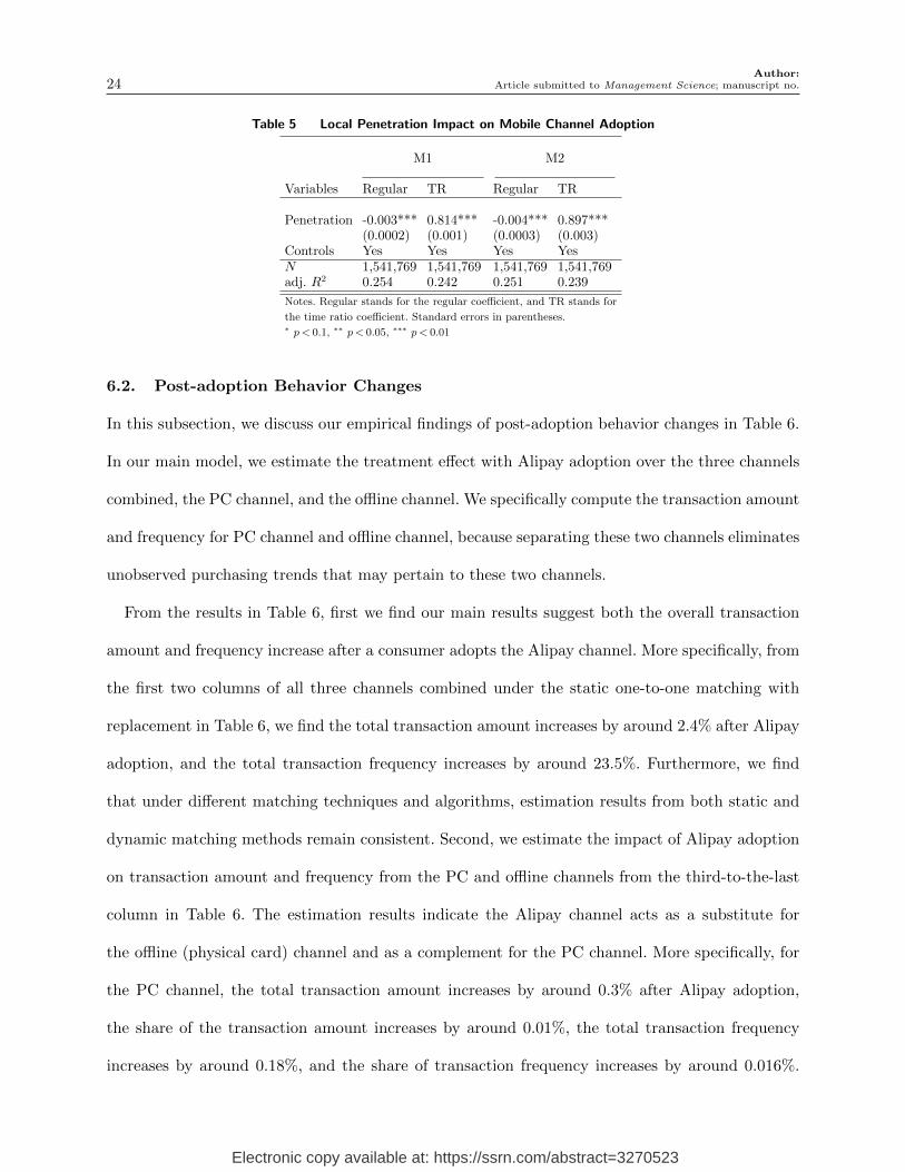
Finally, we discuss the impact of local penetration on mobile channel adoption. The results are
presented in Table 5. Recall that we use the number of existing Alipay adopters within the same
zip code area as the adopter under study to measure the level of local penetration. From results in
Table 5, we find that higher local penetration is associated with earlier mobile channel adoption.
More specifically, a consumer’s time to adopt the mobile payment channel is reduced by around
0.3% with a one-unit increase in the local penetration level (β =−0.003, p < 0.01 for M1).
Electronic copy available at: https://ssrn.com/abstract=3270523
Author:24 Article submitted to Management Science; manuscript no.
Table 5 Local Penetration Impact on Mobile Channel Adoption
M1 M2
Variables Regular TR Regular TR
Penetration -0.003*** 0.814*** -0.004*** 0.897***(0.0002) (0.001) (0.0003) (0.003)
Controls Yes Yes Yes YesN 1,541,769 1,541,769 1,541,769 1,541,769adj. R2 0.254 0.242 0.251 0.239
Notes. Regular stands for the regular coefficient, and TR stands for
the time ratio coefficient. Standard errors in parentheses.∗ p < 0.1, ∗∗ p < 0.05, ∗∗∗ p < 0.01
6.2. Post-adoption Behavior Changes
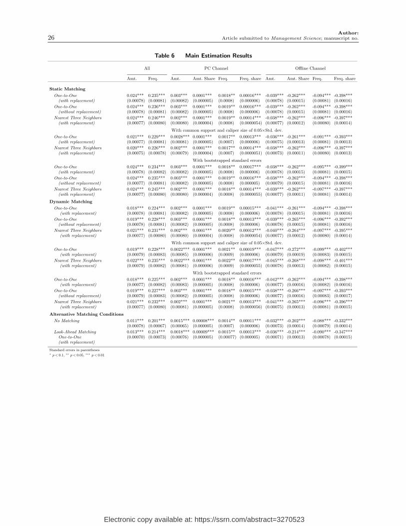
In this subsection, we discuss our empirical findings of post-adoption behavior changes in Table 6.
In our main model, we estimate the treatment effect with Alipay adoption over the three channels
combined, the PC channel, and the offline channel. We specifically compute the transaction amount
and frequency for PC channel and offline channel, because separating these two channels eliminates
unobserved purchasing trends that may pertain to these two channels.
From the results in Table 6, first we find our main results suggest both the overall transaction
amount and frequency increase after a consumer adopts the Alipay channel. More specifically, from
the first two columns of all three channels combined under the static one-to-one matching with
replacement in Table 6, we find the total transaction amount increases by around 2.4% after Alipay
adoption, and the total transaction frequency increases by around 23.5%. Furthermore, we find
that under different matching techniques and algorithms, estimation results from both static and
dynamic matching methods remain consistent. Second, we estimate the impact of Alipay adoption
on transaction amount and frequency from the PC and offline channels from the third-to-the-last
column in Table 6. The estimation results indicate the Alipay channel acts as a substitute for
the offline (physical card) channel and as a complement for the PC channel. More specifically, for
the PC channel, the total transaction amount increases by around 0.3% after Alipay adoption,
the share of the transaction amount increases by around 0.01%, the total transaction frequency
increases by around 0.18%, and the share of transaction frequency increases by around 0.016%.
Electronic copy available at: https://ssrn.com/abstract=3270523

Author:Article submitted to Management Science; manuscript no. 25
On the other hand, for the offline channel, the total transaction amount decreases by around 3.9%
after Alipay adoption, the share of the transaction amount decreases by around 26.2%, the total
transaction frequency decreases by around 9.4%, and the share of transaction frequency decreases
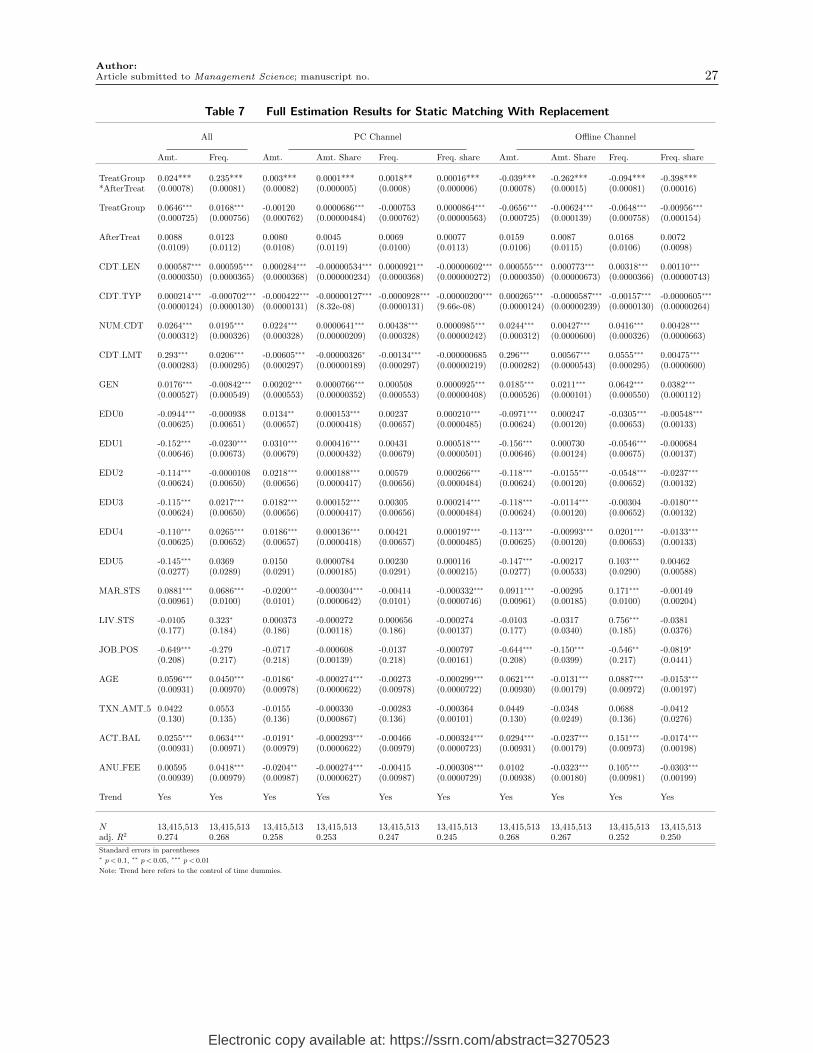
by around 39.8%. We also present our full estimation results of static and dynamic matching with
replacement in Table 7 and 8.
Now we discuss several concerns about our main estimation results. First, we consider the vari-
ance from the estimation of the propensity scores. Following Austin and Small (2014), we bootstrap
the clustered standard errors in the specifications to account for the variance from the estimation of
the propensity scores. Under bootstrapped standard errors, we find the results remain statistically
significant, as shown in Table 6. Furthermore, the positive impact of Alipay adoption is present
where matching is not employed, and also in matched samples derived under the look-ahead match-
ing process, as shown at the bottom of Table 6. Second, interpreting from the baseline models of
one-to-one static and dynamic matching with replacement, we find both the transaction amount
and frequency increase after a consumer utilizes the Alipay channel with her credit card purchase.
However, given the fact that potential hidden bias might exist, matched individuals with the same
observed covariates can have differing probabilities of adopting Alipay, and then can affect the
efficacy of the matching procedure. Thus, we further perform the analysis of Rosenbaum (2002) to
assess the sensitivity of our main results. Such analysis calculates the magnitude of hidden bias that
needs to be present to explain the associations actually observed. The analysis results indicate that
to affect the current results, an unobserved bias needs to produce more than a 1.3-fold increase in
the odds of Alipay adoption and be a strong predictor of outcome variables. Third, the estimation
results may arise due to different pre-existing trends affecting the treatment and control groups.
We then check whether the DID estimates are robust to smaller samples derived from shorter time
windows before and after the release of Alipay. Specifically, we repeat the regressions using samples
that fall within 3, 5, 7, and 9 months before and after the collaboration between our focal bank and
Alipay. The results of this check suggest the main results are not affected by long-term differences
in pre-existing trends.
Electronic copy available at: https://ssrn.com/abstract=3270523
Author:26 Article submitted to Management Science; manuscript no.
Table 6 Main Estimation Results
All PC Channel Offline Channel
Amt. Freq. Amt. Amt. Share Freq. Freq. share Amt. Amt. Share Freq. Freq. share
Static Matching
One-to-One 0.024*** 0.235*** 0.003*** 0.0001*** 0.0018** 0.00016*** -0.039*** -0.262*** -0.094*** -0.398***(with replacement) (0.00078) (0.00081) (0.00082) (0.000005) (0.0008) (0.000006) (0.00078) (0.00015) (0.00081) (0.00016)
One-to-One 0.024*** 0.236*** 0.003*** 0.0001*** 0.0019** 0.00016*** -0.039*** -0.262*** -0.094*** -0.398***(without replacement) (0.00078) (0.00081) (0.00082) (0.000005) (0.0008) (0.000006) (0.00078) (0.00015) (0.00081) (0.00016)
Nearest Three Neighbors 0.024*** 0.246*** 0.002*** 0.0001*** 0.0019** 0.00014*** -0.038*** -0.262*** -0.096*** -0.397***(with replacement) (0.00077) (0.00080) (0.00080) (0.000004) (0.0008) (0.0000054) (0.00077) (0.00012) (0.00080) (0.00014)
With common support and caliper size of 0.05×Std. dev.
One-to-One 0.021*** 0.229*** 0.0028*** 0.0001*** 0.0017** 0.00013*** -0.036*** -0.261*** -0.091*** -0.393***(with replacement) (0.00077) (0.00081) (0.00081) (0.000005) (0.0007) (0.000006) (0.00075) (0.00013) (0.00081) (0.00013)
Nearest Three Neighbors 0.020*** 0.226*** 0.002*** 0.0001*** 0.0017** 0.00014*** -0.038*** -0.262*** -0.096*** -0.397***(with replacement) (0.00075) (0.00078) (0.00079) (0.000004) (0.0007) (0.0000051) (0.00073) (0.00011) (0.00080) (0.00013)
With bootstrapped standard errors
One-to-One 0.024*** 0.234*** 0.003*** 0.0001*** 0.0018** 0.00017*** -0.038*** -0.262*** -0.095*** -0.399***(with replacement) (0.00078) (0.00082) (0.00082) (0.000005) (0.0008) (0.000006) (0.00078) (0.00015) (0.00081) (0.00015)
One-to-One 0.024*** 0.235*** 0.003*** 0.0001*** 0.0019** 0.00016*** -0.038*** -0.262*** -0.094*** -0.398***(without replacement) (0.00077) (0.00081) (0.00082) (0.000005) (0.0008) (0.000005) (0.00079) (0.00015) (0.00081) (0.00016)
Nearest Three Neighbors 0.024*** 0.245*** 0.002*** 0.0001*** 0.0018** 0.00014*** -0.039*** -0.262*** -0.097*** -0.397***(with replacement) (0.00077) (0.00080) (0.00080) (0.000004) (0.0008) (0.0000055) (0.00077) (0.00011) (0.00081) (0.00014)
Dynamic Matching
One-to-One 0.018*** 0.224*** 0.002*** 0.0001*** 0.0019** 0.00015*** -0.041*** -0.261*** -0.094*** -0.398***(with replacement) (0.00078) (0.00081) (0.00082) (0.000005) (0.0008) (0.000006) (0.00078) (0.00015) (0.00081) (0.00016)
One-to-One 0.019*** 0.228*** 0.003*** 0.0001*** 0.0018** 0.00013*** -0.039*** -0.265*** -0.096*** -0.392***(without replacement) (0.00078) (0.00081) (0.00082) (0.000005) (0.0008) (0.000006) (0.00078) (0.00015) (0.00081) (0.00016)
Nearest Three Neighbors 0.021*** 0.231*** 0.002*** 0.0001*** 0.0020** 0.00012*** -0.040*** -0.264*** -0.097*** -0.395***(with replacement) (0.00077) (0.00080) (0.00080) (0.000004) (0.0008) (0.0000054) (0.00077) (0.00012) (0.00080) (0.00014)
With common support and caliper size of 0.05×Std. dev.
One-to-One 0.019*** 0.228*** 0.0022*** 0.0001*** 0.0021** 0.00019*** -0.047*** -0.272*** -0.099*** -0.402***(with replacement) (0.00079) (0.00083) (0.00085) (0.000006) (0.0009) (0.000006) (0.00079) (0.00019) (0.00083) (0.00015)
Nearest Three Neighbors 0.022*** 0.235*** 0.0022*** 0.0001*** 0.0022** 0.00017*** -0.045*** -0.268*** -0.098*** -0.401***(with replacement) (0.00079) (0.00082) (0.00081) (0.000006) (0.0009) (0.0000055) (0.00078) (0.00013) (0.00082) (0.00015)
With bootstrapped standard errors
One-to-One 0.018*** 0.225*** 0.002*** 0.0001*** 0.0018** 0.00016*** -0.042*** -0.262*** -0.094*** -0.398***(with replacement) (0.00077) (0.00082) (0.00083) (0.000005) (0.0008) (0.000006) (0.00077) (0.00016) (0.00082) (0.00016)
One-to-One 0.019*** 0.227*** 0.003*** 0.0001*** 0.0018** 0.00015*** -0.038*** -0.266*** -0.097*** -0.393***(without replacement) (0.00079) (0.00083) (0.00082) (0.000005) (0.0008) (0.000006) (0.00077) (0.00016) (0.00083) (0.00017)
Nearest Three Neighbors 0.021*** 0.232*** 0.002*** 0.0001*** 0.0021** 0.00013*** -0.041*** -0.265*** -0.096*** -0.396***(with replacement) (0.00077) (0.00080) (0.00081) (0.000005) (0.0008) (0.0000056) (0.00075) (0.00013) (0.00081) (0.00015)
Alternative Matching Conditions
No Matching 0.011*** 0.201*** 0.0015*** 0.00008*** 0.0014** 0.00011*** -0.032*** -0.202*** -0.088*** -0.332***(0.00078) (0.00067) (0.00065) (0.000005) (0.0007) (0.000006) (0.00073) (0.00014) (0.00079) (0.00014)
Look-Ahead Matching 0.013*** 0.214*** 0.0018*** 0.00009*** 0.0015** 0.00013*** -0.036*** -0.214*** -0.090*** -0.347***One-to-One (0.00070) (0.00073) (0.00076) (0.000005) (0.00077) (0.000005) (0.00071) (0.00013) (0.00078) (0.00015)(with replacement)
Standard errors in parentheses∗ p < 0.1, ∗∗ p < 0.05, ∗∗∗ p < 0.01
Electronic copy available at: https://ssrn.com/abstract=3270523
Author:Article submitted to Management Science; manuscript no. 27
Table 7 Full Estimation Results for Static Matching With Replacement
All PC Channel Offline Channel
Amt. Freq. Amt. Amt. Share Freq. Freq. share Amt. Amt. Share Freq. Freq. share
TreatGroup 0.024*** 0.235*** 0.003*** 0.0001*** 0.0018** 0.00016*** -0.039*** -0.262*** -0.094*** -0.398****AfterTreat (0.00078) (0.00081) (0.00082) (0.000005) (0.0008) (0.000006) (0.00078) (0.00015) (0.00081) (0.00016)
TreatGroup 0.0646∗∗∗ 0.0168∗∗∗ -0.00120 0.0000686∗∗∗ -0.000753 0.0000864∗∗∗ -0.0656∗∗∗ -0.00624∗∗∗ -0.0648∗∗∗ -0.00956∗∗∗
(0.000725) (0.000756) (0.000762) (0.00000484) (0.000762) (0.00000563) (0.000725) (0.000139) (0.000758) (0.000154)
AfterTreat 0.0088 0.0123 0.0080 0.0045 0.0069 0.00077 0.0159 0.0087 0.0168 0.0072(0.0109) (0.0112) (0.0108) (0.0119) (0.0100) (0.0113) (0.0106) (0.0115) (0.0106) (0.0098)
CDT LEN 0.000587∗∗∗ 0.000595∗∗∗ 0.000284∗∗∗ -0.00000534∗∗∗ 0.0000921∗∗ -0.00000602∗∗∗ 0.000555∗∗∗ 0.000773∗∗∗ 0.00318∗∗∗ 0.00110∗∗∗
(0.0000350) (0.0000365) (0.0000368) (0.000000234) (0.0000368) (0.000000272) (0.0000350) (0.00000673) (0.0000366) (0.00000743)
CDT TYP 0.000214∗∗∗ -0.000702∗∗∗ -0.000422∗∗∗ -0.00000127∗∗∗ -0.0000928∗∗∗ -0.00000200∗∗∗ 0.000265∗∗∗ -0.0000587∗∗∗ -0.00157∗∗∗ -0.0000605∗∗∗
(0.0000124) (0.0000130) (0.0000131) (8.32e-08) (0.0000131) (9.66e-08) (0.0000124) (0.00000239) (0.0000130) (0.00000264)
NUM CDT 0.0264∗∗∗ 0.0195∗∗∗ 0.0224∗∗∗ 0.0000641∗∗∗ 0.00438∗∗∗ 0.0000985∗∗∗ 0.0244∗∗∗ 0.00427∗∗∗ 0.0416∗∗∗ 0.00428∗∗∗
(0.000312) (0.000326) (0.000328) (0.00000209) (0.000328) (0.00000242) (0.000312) (0.0000600) (0.000326) (0.0000663)
CDT LMT 0.293∗∗∗ 0.0206∗∗∗ -0.00605∗∗∗ -0.00000326∗ -0.00134∗∗∗ -0.000000685 0.296∗∗∗ 0.00567∗∗∗ 0.0555∗∗∗ 0.00475∗∗∗
(0.000283) (0.000295) (0.000297) (0.00000189) (0.000297) (0.00000219) (0.000282) (0.0000543) (0.000295) (0.0000600)
GEN 0.0176∗∗∗ -0.00842∗∗∗ 0.00202∗∗∗ 0.0000766∗∗∗ 0.000508 0.0000925∗∗∗ 0.0185∗∗∗ 0.0211∗∗∗ 0.0642∗∗∗ 0.0382∗∗∗
(0.000527) (0.000549) (0.000553) (0.00000352) (0.000553) (0.00000408) (0.000526) (0.000101) (0.000550) (0.000112)
EDU0 -0.0944∗∗∗ -0.000938 0.0134∗∗ 0.000153∗∗∗ 0.00237 0.000210∗∗∗ -0.0971∗∗∗ 0.000247 -0.0305∗∗∗ -0.00548∗∗∗
(0.00625) (0.00651) (0.00657) (0.0000418) (0.00657) (0.0000485) (0.00624) (0.00120) (0.00653) (0.00133)
EDU1 -0.152∗∗∗ -0.0230∗∗∗ 0.0310∗∗∗ 0.000416∗∗∗ 0.00431 0.000518∗∗∗ -0.156∗∗∗ 0.000730 -0.0546∗∗∗ -0.000684(0.00646) (0.00673) (0.00679) (0.0000432) (0.00679) (0.0000501) (0.00646) (0.00124) (0.00675) (0.00137)
EDU2 -0.114∗∗∗ -0.0000108 0.0218∗∗∗ 0.000188∗∗∗ 0.00579 0.000266∗∗∗ -0.118∗∗∗ -0.0155∗∗∗ -0.0548∗∗∗ -0.0237∗∗∗
(0.00624) (0.00650) (0.00656) (0.0000417) (0.00656) (0.0000484) (0.00624) (0.00120) (0.00652) (0.00132)
EDU3 -0.115∗∗∗ 0.0217∗∗∗ 0.0182∗∗∗ 0.000152∗∗∗ 0.00305 0.000214∗∗∗ -0.118∗∗∗ -0.0114∗∗∗ -0.00304 -0.0180∗∗∗
(0.00624) (0.00650) (0.00656) (0.0000417) (0.00656) (0.0000484) (0.00624) (0.00120) (0.00652) (0.00132)
EDU4 -0.110∗∗∗ 0.0265∗∗∗ 0.0186∗∗∗ 0.000136∗∗∗ 0.00421 0.000197∗∗∗ -0.113∗∗∗ -0.00993∗∗∗ 0.0201∗∗∗ -0.0133∗∗∗
(0.00625) (0.00652) (0.00657) (0.0000418) (0.00657) (0.0000485) (0.00625) (0.00120) (0.00653) (0.00133)
EDU5 -0.145∗∗∗ 0.0369 0.0150 0.0000784 0.00230 0.000116 -0.147∗∗∗ -0.00217 0.103∗∗∗ 0.00462(0.0277) (0.0289) (0.0291) (0.000185) (0.0291) (0.000215) (0.0277) (0.00533) (0.0290) (0.00588)
MAR STS 0.0881∗∗∗ 0.0686∗∗∗ -0.0200∗∗ -0.000304∗∗∗ -0.00414 -0.000332∗∗∗ 0.0911∗∗∗ -0.00295 0.171∗∗∗ -0.00149(0.00961) (0.0100) (0.0101) (0.0000642) (0.0101) (0.0000746) (0.00961) (0.00185) (0.0100) (0.00204)
LIV STS -0.0105 0.323∗ 0.000373 -0.000272 0.000656 -0.000274 -0.0103 -0.0317 0.756∗∗∗ -0.0381(0.177) (0.184) (0.186) (0.00118) (0.186) (0.00137) (0.177) (0.0340) (0.185) (0.0376)
JOB POS -0.649∗∗∗ -0.279 -0.0717 -0.000608 -0.0137 -0.000797 -0.644∗∗∗ -0.150∗∗∗ -0.546∗∗ -0.0819∗
(0.208) (0.217) (0.218) (0.00139) (0.218) (0.00161) (0.208) (0.0399) (0.217) (0.0441)
AGE 0.0596∗∗∗ 0.0450∗∗∗ -0.0186∗ -0.000274∗∗∗ -0.00273 -0.000299∗∗∗ 0.0621∗∗∗ -0.0131∗∗∗ 0.0887∗∗∗ -0.0153∗∗∗
(0.00931) (0.00970) (0.00978) (0.0000622) (0.00978) (0.0000722) (0.00930) (0.00179) (0.00972) (0.00197)
TXN AMT 5 0.0422 0.0553 -0.0155 -0.000330 -0.00283 -0.000364 0.0449 -0.0348 0.0688 -0.0412(0.130) (0.135) (0.136) (0.000867) (0.136) (0.00101) (0.130) (0.0249) (0.136) (0.0276)
ACT BAL 0.0255∗∗∗ 0.0634∗∗∗ -0.0191∗ -0.000293∗∗∗ -0.00466 -0.000324∗∗∗ 0.0294∗∗∗ -0.0237∗∗∗ 0.151∗∗∗ -0.0174∗∗∗
(0.00931) (0.00971) (0.00979) (0.0000622) (0.00979) (0.0000723) (0.00931) (0.00179) (0.00973) (0.00198)
ANU FEE 0.00595 0.0418∗∗∗ -0.0204∗∗ -0.000274∗∗∗ -0.00415 -0.000308∗∗∗ 0.0102 -0.0323∗∗∗ 0.105∗∗∗ -0.0303∗∗∗
(0.00939) (0.00979) (0.00987) (0.0000627) (0.00987) (0.0000729) (0.00938) (0.00180) (0.00981) (0.00199)
Trend Yes Yes Yes Yes Yes Yes Yes Yes Yes Yes
N 13,415,513 13,415,513 13,415,513 13,415,513 13,415,513 13,415,513 13,415,513 13,415,513 13,415,513 13,415,513adj. R2 0.274 0.268 0.258 0.253 0.247 0.245 0.268 0.267 0.252 0.250
Standard errors in parentheses∗ p < 0.1, ∗∗ p < 0.05, ∗∗∗ p < 0.01
Note: Trend here refers to the control of time dummies.
Electronic copy available at: https://ssrn.com/abstract=3270523

Author:28 Article submitted to Management Science; manuscript no.
Table 8 Full Estimation Results for Dynamic Matching With Replacement
All PC Channel Offline Channel
Amt. Freq. Amt. Amt. Share Freq. Freq. share Amt. Amt. Share Freq. Freq. share
TreatGroup 0.018*** 0.224*** 0.002*** 0.0001*** 0.0019** 0.00015*** -0.041*** -0.261*** -0.094*** -0.398****AfterTreat (0.00078) (0.00081) (0.00082) (0.000005) (0.0008) (0.000006) (0.00078) (0.00015) (0.00081) (0.00016)
TreatGroup 0.0445∗∗∗ -0.00431∗∗∗ -0.00122 0.0000567∗∗∗ -0.000928 0.0000724∗∗∗ 0.0451∗∗∗ 0.00818∗∗∗ 0.0128∗∗∗ 0.0117∗∗∗
(0.000740) (0.000766) (0.000771) (0.00000503) (0.000772) (0.00000588) (0.000740) (0.000142) (0.000766) (0.000157)
AfterTreat 0.0069 0.0117 0.0092 0.0051 0.0073 0.00101 0.0143 0.0089 0.0155 0.0081(0.0111) (0.0113) (0.0112) (0.0106) (0.0109) (0.0106) (0.0116) (0.0108) (0.0107) (0.0093)
CDT LEN 0.000315∗∗∗ 0.000935∗∗∗ 0.000300∗∗∗ -0.00000625∗∗∗ 0.0000987∗∗∗ -0.00000704∗∗∗ 0.000286∗∗∗ 0.000792∗∗∗ 0.00413∗∗∗ 0.00113∗∗∗
(0.0000359) (0.0000371) (0.0000374) (0.000000244) (0.0000374) (0.000000285) (0.0000359) (0.00000688) (0.0000371) (0.00000760)
CDT TYP 0.000168∗∗∗ -0.000694∗∗∗ -0.000383∗∗∗ -0.000000971∗∗∗ -0.0000988∗∗∗ -0.00000166∗∗∗ 0.000207∗∗∗ -0.0000238∗∗∗ -0.00156∗∗∗ -0.0000244∗∗∗
(0.0000122) (0.0000126) (0.0000127) (8.29e-08) (0.0000127) (9.68e-08) (0.0000122) (0.00000234) (0.0000126) (0.00000258)
NUM CDT 0.0438∗∗∗ 0.0318∗∗∗ 0.0236∗∗∗ 0.0000538∗∗∗ 0.00481∗∗∗ 0.0000905∗∗∗ 0.0423∗∗∗ 0.00307∗∗∗ 0.0739∗∗∗ 0.00305∗∗∗
(0.000299) (0.000310) (0.000312) (0.00000204) (0.000312) (0.00000238) (0.000299) (0.0000574) (0.000310) (0.0000634)
CDT LMT 0.261∗∗∗ 0.0143∗∗∗ -0.00570∗∗∗ -0.00000103 -0.00135∗∗∗ 0.00000107 0.264∗∗∗ 0.00495∗∗∗ 0.0403∗∗∗ 0.00415∗∗∗
(0.000283) (0.000293) (0.000295) (0.00000192) (0.000295) (0.00000225) (0.000283) (0.0000542) (0.000293) (0.0000599)
GEN 0.0189∗∗∗ -0.00744∗∗∗ 0.00174∗∗∗ 0.0000802∗∗∗ 0.00176∗∗∗ 0.0000962∗∗∗ 0.0197∗∗∗ 0.0214∗∗∗ 0.0615∗∗∗ 0.0387∗∗∗
(0.000534) (0.000553) (0.000557) (0.00000363) (0.000557) (0.00000424) (0.000534) (0.000102) (0.000553) (0.000113)
EDU0 -0.0874∗∗∗ -0.0242∗∗∗ 0.0170∗∗∗ 0.000144∗∗∗ 0.00551 0.000205∗∗∗ -0.0900∗∗∗ 0.000849 -0.0948∗∗∗ -0.00407∗∗∗
(0.00595) (0.00616) (0.00620) (0.0000405) (0.00620) (0.0000472) (0.00595) (0.00114) (0.00615) (0.00126)
EDU1 -0.139∗∗∗ -0.0520∗∗∗ 0.0377∗∗∗ 0.000469∗∗∗ 0.00492 0.000590∗∗∗ -0.143∗∗∗ 0.000156 -0.135∗∗∗ -0.000918(0.00616) (0.00638) (0.00642) (0.0000419) (0.00642) (0.0000489) (0.00616) (0.00118) (0.00637) (0.00130)
EDU2 -0.111∗∗∗ -0.0340∗∗∗ 0.0228∗∗∗ 0.000173∗∗∗ 0.00581 0.000252∗∗∗ -0.114∗∗∗ -0.0155∗∗∗ -0.141∗∗∗ -0.0229∗∗∗
(0.00594) (0.00615) (0.00619) (0.0000404) (0.00619) (0.0000472) (0.00594) (0.00114) (0.00614) (0.00126)
EDU3 -0.110∗∗∗ -0.0146∗∗ 0.0183∗∗∗ 0.000134∗∗∗ 0.00321 0.000197∗∗∗ -0.113∗∗∗ -0.0117∗∗∗ -0.0936∗∗∗ -0.0175∗∗∗
(0.00594) (0.00615) (0.00619) (0.0000404) (0.00619) (0.0000472) (0.00594) (0.00114) (0.00614) (0.00126)
EDU4 -0.105∗∗∗ -0.0109∗ 0.0196∗∗∗ 0.000121∗∗∗ 0.00351 0.000183∗∗∗ -0.107∗∗∗ -0.0102∗∗∗ -0.0715∗∗∗ -0.0128∗∗∗
(0.00595) (0.00616) (0.00620) (0.0000405) (0.00620) (0.0000473) (0.00595) (0.00114) (0.00616) (0.00126)
EDU5 -0.135∗∗∗ -0.0195 0.0148 0.0000666 0.00227 0.000103 -0.137∗∗∗ -0.00190 -0.0356 0.00719(0.0281) (0.0291) (0.0293) (0.000191) (0.0293) (0.000223) (0.0281) (0.00539) (0.0291) (0.00595)
MAR STS 0.0494∗∗∗ 0.0943∗∗∗ -0.0214∗∗ -0.000274∗∗∗ -0.00497 -0.000313∗∗∗ 0.0515∗∗∗ -0.00143 0.246∗∗∗ -0.00116(0.00917) (0.00949) (0.00955) (0.0000623) (0.00955) (0.0000728) (0.00916) (0.00176) (0.00948) (0.00194)
LIV STS -0.0628 0.338 -0.00623 -0.000256 -0.00396 -0.000294 -0.0630 -0.0335 0.826∗∗∗ -0.0405(0.248) (0.257) (0.258) (0.00174) (0.258) (0.00197) (0.248) (0.0492) (0.256) (0.0525)
JOB POS -0.228 0.0469 -0.0336 -0.000399 -0.00920 -0.000494 -0.227 -0.0793∗∗∗ 0.181 -0.0499∗
(0.142) (0.147) (0.148) (0.000964) (0.148) (0.00113) (0.142) (0.0272) (0.147) (0.0300)
AGE 0.0255∗∗∗ 0.0735∗∗∗ -0.0193∗∗ -0.000249∗∗∗ -0.00339 -0.000280∗∗∗ 0.0273∗∗∗ -0.0118∗∗∗ 0.169∗∗∗ -0.0153∗∗∗
(0.00883) (0.00914) (0.00920) (0.0000600) (0.00920) (0.0000701) (0.00883) (0.00169) (0.00913) (0.00187)
TXN AMT 5 -0.0940 0.00643 -0.0181 -0.000294 -0.00708 -0.000330 -0.0933 -0.0281 -0.0299 -0.0325(0.220) (0.228) (0.230) (0.00150) (0.230) (0.00175) (0.220) (0.0422) (0.228) (0.0467)
ACT BAL -0.00921 0.0886∗∗∗ -0.0200∗∗ -0.000264∗∗∗ -0.00542 -0.000302∗∗∗ -0.00630 -0.0229∗∗∗ 0.224∗∗∗ -0.0176∗∗∗
(0.00884) (0.00915) (0.00921) (0.0000601) (0.00921) (0.0000702) (0.00884) (0.00170) (0.00915) (0.00187)
ANU FEE -0.0300∗∗∗ 0.0642∗∗∗ -0.0228∗∗ -0.000253∗∗∗ -0.00650 -0.000294∗∗∗ -0.0268∗∗∗ -0.0308∗∗∗ 0.172∗∗∗ -0.0301∗∗∗
(0.00892) (0.00923) (0.00929) (0.0000606) (0.00930) (0.0000708) (0.00892) (0.00171) (0.00923) (0.00189)
Trend Yes Yes Yes Yes Yes Yes Yes Yes Yes Yes
N 13,302,196 13,302,196 13,302,196 13,302,196 13,302,196 13,302,196 13,302,196 13,302,196 13,302,196 13,302,196adj. R2 0.286 0.280 0.272 0.270 0.265 0.262 0.281 0.279 0.272 0.271
Standard errors in parentheses∗ p < 0.1, ∗∗ p < 0.05, ∗∗∗ p < 0.01
Note: Trend here refers to the control of time dummies.
Electronic copy available at: https://ssrn.com/abstract=3270523

Author:Article submitted to Management Science; manuscript no. 29
6.3. Post-adoption: Subset Analysis
In this subsection, we try to explore the driven forces of the increasing transaction amount and fre-
quency. We conduct subset analysis based on purchasing product category and value, and consumer
credit limit level and observation periods.
Product Category. Based on the practice of our focal bank, the credit card department classifies
consumer purchasing products into six categories as shown in the following Table 9. We can see that
grocery shopping has the highest consumption frequency in our data set, followed by education and
entertainment. Intuitively, service, entertainment, groceries, and travel are more related to hedonic
shopping. To examine the impact of mobile channel adoption on the consumption for each category,
we compute the total consumption amount, frequency, and shares of different channels for each of
the six product categories, and then conduct our DID analysis for each category separately and show
our results in Table 10. From the results in Table 10, we can see that both the overall consumption
amount and frequency increase for groceries, entertainment, travel, and service categories. Second,
for these four categories, the complementarity and substitution effects still hold. Third, mobile
channel adoption affects the groceries category the most, followed by the entertainment, travel,
and service categories. Finally, mobile channel adoption seems unlikely to affect education and
healthcare categories, because the estimated coefficients are not statistically significant with our
data set.
Table 9 Consumption Categories
Category Definition Number PercentageEducation School education, professional training, etc. 16,193,466 14.84%Service Cleaning, repairing, etc. 1,462,219 1.34%Healthcare Hospital service, medicine, etc. 1,002,069 0.92%Entertainment Restaurant, gym, etc. 4,326,357 3.96%Groceries Supermarket, wholesale, etc. 43,122,235 39.51%Travel Flight ticket, hotel rooms, subway, etc. 3,832,095 3.51%
Electronic copy available at: https://ssrn.com/abstract=3270523

Author:30 Article submitted to Management Science; manuscript no.
Table 10 Impacts under Different Consumption Categories
All PC Channel Offline Channel
Amt. Freq. Amt. Amt. Share Freq. Freq. share Amt. Amt. Share Freq. Freq. share
Education
Static One-to-One 0.023 0.248 0.007 0.0009 0.0010 0.00022 -0.043 -0.277 -0.091 -0.366(with replacement) (0.03289) (0.27856) (0.04468) (0.005497) (0.04125) (0.005478) (0.034879) (0.26547) (0.13566) (0.35811)
Dynamic One-to-One 0.025 0.223 0.012 0.0015 0.0028 0.00014 -0.038 -0.271 -0.088 -0.361(with replacement) (0.03256) (0.25578) (0.07588) (0.005469) (0.04283) (0.008267) (0.03167) (0.34879) (0.23647) (0.37945)
Service
Static One-to-One 0.038** 0.272*** 0.002*** 0.0005*** 0.0013** 0.00011*** -0.022*** -0.233*** -0.064*** -0.375***(with replacement) (0.00111) (0.00105) (0.00095) (0.000007) (0.0011) (0.000013) (0.00092) (0.00015) (0.00088) (0.00020)
Dynamic One-to-One 0.033** 0.270*** 0.001*** 0.0004*** 0.0011** 0.00009*** -0.020*** -0.231*** -0.062*** -0.371***(with replacement) (0.00113) (0.00102) (0.00091) (0.000005) (0.0021) (0.000011) (0.00087) (0.00012) (0.00082) (0.00017)
Healthcare
Static One-to-One 0.038 0.257 0.011 0.0013 0.0019 0.00017 -0.042 -0.273 -0.088 -0.355(with replacement) (0.03789) (0.24756) (0.04257) (0.005968) (0.04478) (0.005649) (0.034731) (0.27619) (0.16791) (0.36715)
Dynamic One-to-One 0.033 0.249 0.010 0.0012 0.0015 0.00013 -0.031 -0.255 -0.080 -0.352(with replacement) (0.03487) (0.22496) (0.08472) (0.006284) (0.05874) (0.008964) (0.03547) (0.35789) (0.26478) (0.34982)
Entertainment
Static One-to-One 0.049*** 0.294*** 0.011*** 0.0014*** 0.0022** 0.00020*** -0.031*** -0.256*** -0.092*** -0.397***(with replacement) (0.00102) (0.00117) (0.00105) (0.000012) (0.0015) (0.000016) (0.00096) (0.00021) (0.00095) (0.00021)
Dynamic One-to-One 0.043*** 0.281*** 0.007*** 0.0011*** 0.0022** 0.00019*** -0.028*** -0.232*** -0.089*** -0.387***(with replacement) (0.00103) (0.00109) (0.00108) (0.000010) (0.0007) (0.000019) (0.00092) (0.00018) (0.00087) (0.00019)
Groceries
Static One-to-One 0.052*** 0.302*** 0.012*** 0.0018*** 0.0027** 0.00024*** -0.033*** -0.271*** -0.099*** -0.402***(with replacement) (0.00105) (0.00121) (0.00108) (0.000010) (0.0012) (0.000017) (0.00099) (0.00022) (0.00096) (0.00024)
Dynamic One-to-One 0.047*** 0.284*** 0.009*** 0.0013*** 0.0025** 0.00021*** -0.031*** -0.265*** -0.091*** -0.392***(with replacement) (0.00101) (0.00114) (0.00102) (0.000009) (0.0010) (0.000016) (0.00094) (0.00021) (0.00092) (0.00022)
Travel
Static One-to-One 0.041** 0.278*** 0.006*** 0.0011*** 0.0017** 0.00015*** -0.027*** -0.249*** -0.087*** -0.390***(with replacement) (0.00108) (0.00111) (0.00102) (0.000009) (0.0013) (0.000019) (0.00099) (0.00018) (0.00093) (0.00025)
Dynamic One-to-One 0.038*** 0.277*** 0.004*** 0.0009*** 0.0016** 0.00014*** -0.023*** -0.235*** -0.081*** -0.382***(with replacement) (0.00096) (0.00101) (0.00112) (0.000014) (0.0010) (0.000023) (0.00098) (0.00015) (0.00089) (0.00023)
Standard errors in parentheses∗ p < 0.1, ∗∗ p < 0.05, ∗∗∗ p < 0.01
Product Value. We next classify the product value into six value categories: less than 100 RMB,
100 to 500 RMB, 500 to 1,000 RMB, 1,000 to 5,000 RMB, 5,000 to 10,000 RMB, and more than
10,000 RMB. Again, to examine the impact of mobile channel adoption on the consumption for
different value categories, we compute the total consumption amount, frequency and shares of
different channels for each of the six product categories, and then conduct our DID analysis for each
value level separately and show our results in Table 11. From the results in Table 11, we can see
that both overall consumption amount and frequency increase for products less than 10,000 RMB,
and the complementarity and substitution effects still hold for these products. Second, the mobile
channel adoption has the greatest effect on low-value items priced at less than 100 RMB, followed
by 100 to 500 RMB, and 500 to 1,000 RMB items. The impacts on items with values less than
Electronic copy available at: https://ssrn.com/abstract=3270523

Author:Article submitted to Management Science; manuscript no. 31
1,000 to 5,000 RMB and 5,000 to 10,000 RMB seem to be similar. Finally, mobile channel adoption
seems unlikely to affect high-value items priced at more than 10,000 RMB, because the estimated
coefficients are not statistically significant with our data set. Combining the subset analysis results
of product category and value, we find that the increased credit card transaction activity and
profitability are likely to be driven by hedonic shopping behavior with low value items.
Table 11 Impacts under Different Product Values
All PC Channel Offline Channel
Amt. Freq. Amt. Amt. Share Freq. Freq. share Amt. Amt. Share Freq. Freq. share
Less than 100 RMB
Static One-to-One 0.055*** 0.317*** 0.016*** 0.0028*** 0.0033*** 0.00045*** -0.067*** -0.311*** -0.124*** -0.421***(with replacement) (0.00102) (0.00097) (0.00111) (0.000022) (0.0012) (0.000017) (0.00099) (0.00022) (0.00098) (0.00033)
Dynamic One-to-One 0.051*** 0.312*** 0.014*** 0.0025*** 0.0030*** 0.00041*** -0.062*** -0.308*** -0.121*** -0.417***(with replacement) (0.00099) (0.00091) (0.00102) (0.000020) (0.0010) (0.000011) (0.00095) (0.00020) (0.00091) (0.00030)
100 to 500 RMB
Static One-to-One 0.050*** 0.311*** 0.012*** 0.0021*** 0.0030*** 0.00042*** -0.063*** -0.302*** -0.111*** -0.406***(with replacement) (0.00099) (0.00088) (0.00103) (0.000020) (0.0011) (0.000014) (0.00094) (0.00012) (0.00090) (0.00031)
Dynamic One-to-One 0.047*** 0.302*** 0.010*** 0.0017*** 0.0028*** 0.00039*** -0.060*** -0.297*** -0.106*** -0.398***(with replacement) (0.00094) (0.00081) (0.00100) (0.000019) (0.0009) (0.000011) (0.00092) (0.00010) (0.00088) (0.00028)
500 to 1,000 RMB
Static One-to-One 0.041*** 0.297*** 0.010*** 0.0018*** 0.0024*** 0.00037*** -0.058*** -0.287*** -0.100*** -0.387***(with replacement) (0.00077) (0.00062) (0.00087) (0.000015) (0.0008) (0.000010) (0.00090) (0.00009) (0.00081) (0.00022)
Dynamic One-to-One 0.039*** 0.290*** 0.009*** 0.0016*** 0.0021*** 0.00035*** -0.053*** -0.284*** -0.098*** -0.380***(with replacement) (0.00075) (0.00060) (0.00085) (0.000012) (0.0007) (0.000009) (0.00082) (0.00008) (0.00077) (0.00020)
1,000 to 5,000 RMB
Static One-to-One 0.028*** 0.239*** 0.005*** 0.0007*** 0.0016** 0.00019*** -0.042*** -0.266*** -0.097*** -0.405***(with replacement) (0.00098) (0.00087) (0.00085) (0.000009) (0.0010) (0.000009) (0.00083) (0.00019) (0.00087) (0.00018)
Dynamic One-to-One 0.024*** 0.235*** 0.004*** 0.0006*** 0.0014** 0.00017*** -0.040*** -0.265*** -0.095*** -0.403***(with replacement) (0.00095) (0.00085) (0.00084) (0.000008) (0.0009) (0.000007) (0.00081) (0.00017) (0.00085) (0.00016)
5,000 to 10,000 RMB
Static One-to-One 0.027*** 0.238*** 0.005*** 0.0006*** 0.0016** 0.00018*** -0.041*** -0.265*** -0.093*** -0.397***(with replacement) (0.00077) (0.00079) (0.00080) (0.000004) (0.0006) (0.000005) (0.00075) (0.00014) (0.00080) (0.00015)
Dynamic One-to-One 0.019*** 0.223*** 0.004*** 0.0005*** 0.0015** 0.00016*** -0.040*** -0.258*** -0.091*** -0.395***(with replacement) (0.00074) (0.00080) (0.00084) (0.000007) (0.0009) (0.000005) (0.00075) (0.00012) (0.00080) (0.00014)
More than 10,000 RMB
Static One-to-One 0.044 0.267 0.005 0.0006 0.0023 0.00019 -0.035 -0.260 -0.090 -0.395(with replacement) (0.04268) (0.27854) (0.00554) (0.000789) (0.0087) (0.000257) (0.02478) (0.25879) (0.09978) (0.32568)
Dynamic One-to-One 0.041 0.260 0.002 0.0004 0.0020 0.00015 -0.032 -0.255 -0.081 -0.390(with replacement) (0.04546) (0.29945) (0.00658) (0.000812) (0.0098) (0.000325) (0.02587) (0.25647) (0.09358) (0.31578)
Standard errors in parentheses∗ p < 0.1, ∗∗ p < 0.05, ∗∗∗ p < 0.01
Credit Limit. Banks normally determine consumers’ credit limits based on their consumption
ability and income level. Note that here we do not use income data directly because: (i) in China, the
income data are generally self-reported and thus not very reliable; and (ii) a lot of consumers choose
not to release their income, so we see only a small percentage of consumers’ income in our data
set. Moreover, under real banking practice in China, the credit limit is a good proxy for consumer
Electronic copy available at: https://ssrn.com/abstract=3270523

Author:32 Article submitted to Management Science; manuscript no.
income level. We hence separate consumers into different credit-limit percentage categories: bottom
25%, 25% to 50%, 50% to 75%, and top 25%. We show our estimation results in Table 12. Based
on the results in Table 12, we find all the effects remain consistent with our main estimation.
Furthermore, we find that Alipay adoption has a greater impact on consumers with medium credit-
limit levels (i.e., middle 25% to 50% and 50% to 75% categories) than on consumers with the
lowest and highest credit-limit levels. Therefore, we would expect that the positive relationship
between mobile channel adoption and increased credit card transaction activity and profitability is
even stronger for medium income consumers. This subset analysis also checks whether the causal
effects are due to actual usage of Alipay or an artifact driven by unobserved characteristics such
as disposable income. Although the dynamic matching method that takes into account consumers’
behavior over time might alleviate this concern to a certain extent, this subset analysis further
reduces this concern.
Table 12 Credit Limit Subsets Analysis
All PC Channel Offline Channel
Amt. Freq. Amt. Amt. Share Freq. Freq. share Amt. Amt. Share Freq. Freq. share
Bottom 25%
Static One-to-One 0.021*** 0.230*** 0.003*** 0.0005*** 0.0011** 0.00012*** -0.033*** -0.258*** -0.088*** -0.383***(with replacement) (0.00081) (0.00079) (0.00078) (0.000006) (0.0008) (0.000006) (0.00077) (0.00015) (0.00081) (0.00014)
Dynamic One-to-One 0.018*** 0.227*** 0.002*** 0.0004*** 0.0009** 0.00011*** -0.031*** -0.256*** -0.085*** -0.381***(with replacement) (0.00079) (0.00073) (0.00072) (0.000005) (0.0007) (0.000004) (0.00072) (0.00011) (0.00080) (0.00013)
25% to 50%
Static One-to-One 0.032*** 0.243*** 0.009*** 0.0012*** 0.0019** 0.00021*** -0.047*** -0.278*** -0.106*** -0.408***(with replacement) (0.00098) (0.00095) (0.00093) (0.000013) (0.0017) (0.000015) (0.00096) (0.00029) (0.00100) (0.00028)
Dynamic One-to-One 0.030*** 0.241*** 0.007*** 0.0011*** 0.0017** 0.00020*** -0.045*** -0.276*** -0.104*** -0.406***(with replacement) (0.00091) (0.00090) (0.00089) (0.000011) (0.0015) (0.000013) (0.00092) (0.00027) (0.00096) (0.00024)
50% to 75%
Static One-to-One 0.040*** 0.255** 0.018*** 0.0025*** 0.0030** 0.00036*** -0.059*** -0.288*** -0.118*** -0.420***(with replacement) (0.00105) (0.00101) (0.00099) (0.000024) (0.0028) (0.000022) (0.00100) (0.00037) (0.00112) (0.00043)
Dynamic One-to-One 0.038*** 0.251** 0.017*** 0.0023*** 0.0027** 0.00034*** -0.057*** -0.286*** -0.115*** -0.417***(with replacement) (0.00101) (0.00096) (0.00093) (0.000022) (0.0026) (0.000020) (0.00091) (0.00033) (0.00108) (0.00041)
Top 25%
Static One-to-One 0.025*** 0.234*** 0.005*** 0.0007*** 0.0015** 0.00016*** -0.039*** -0.262*** -0.097*** -0.396***(with replacement) (0.00089) (0.00083) (0.00082) (0.000009) (0.0011) (0.000009) (0.00085) (0.00019) (0.00090) (0.00018)
Dynamic One-to-One 0.022*** 0.231*** 0.004*** 0.0006*** 0.0013** 0.00013*** -0.036*** -0.260*** -0.095*** -0.392***(with replacement) (0.00083) (0.00080) (0.00079) (0.000008) (0.0010) (0.000007) (0.00083) (0.00017) (0.00088) (0.00016)
Standard errors in parentheses∗ p < 0.1, ∗∗ p < 0.05, ∗∗∗ p < 0.01
Observation Periods. To understand both short- and long-run impact of Alipay adoption, we
separate our data set into different observation periods. Recalling that we have 29 months of data,
Electronic copy available at: https://ssrn.com/abstract=3270523

Author:Article submitted to Management Science; manuscript no. 33
from September 2010 to February 2013, we now classify our data set into the following categories:
1st to 6th month, 6th to 12th month, 13th to 18th month, 19th to 24th month, and 25th to 29th
month. We show our estimation results in Table 13. Based on the results in Table 13, we find all
the effects remain consistent with our main estimation. Furthermore, we find the impacts of Alipay
adoption on both the PC and physical card channels increase over time, and the impact on the
physical card channel increases more significantly as time passes as compared to the PC payment
channel. Finally, this subset analysis also reduces the concern that our main results might be driven
by the improved performance efficiency of the Alipay app and added features in new versions (as
a new startup company in China, Alipay has been continuously improving its app functions).
Table 13 Time Periods Subsets Analysis
All PC Channel Offline Channel
Amt. Freq. Amt. Amt. Share Freq. Freq. share Amt. Amt. Share Freq. Freq. share
1st to 6th month
Static One-to-One 0.013*** 0.106*** 0.009*** 0.0011*** 0.0012*** 0.00018*** -0.029*** -0.108*** -0.087*** -0.177***(with replacement) (0.00041) (0.00072) (0.00085) (0.000013) (0.0009) (0.000010) (0.00076) (0.00014) (0.00074) (0.00012)
Dynamic One-to-One 0.011*** 0.102*** 0.008*** 0.0009*** 0.0011*** 0.00016*** -0.027*** -0.104*** -0.082*** -0.173***(with replacement) (0.00040) (0.00069) (0.00082) (0.000011) (0.0008) (0.000008) (0.00072) (0.00012) (0.00071) (0.00011)
6th to 12th month
Static One-to-One 0.023*** 0.120*** 0.012*** 0.0019*** 0.0017*** 0.00022*** -0.044*** -0.137*** -0.101*** -0.203***(with replacement) (0.00055) (0.00079) (0.00089) (0.000014) (0.0012) (0.000011) (0.00079) (0.00015) (0.00077) (0.00014)
Dynamic One-to-One 0.021*** 0.118*** 0.011*** 0.0017*** 0.0015*** 0.00020*** -0.042*** -0.135*** -0.100*** -0.199***(with replacement) (0.00052) (0.00075) (0.00086) (0.000013) (0.0012) (0.000010) (0.00076) (0.00014) (0.00073) (0.00012)
13th to 18th month
Static One-to-One 0.032*** 0.134*** 0.019*** 0.0026*** 0.0023*** 0.00031*** -0.067*** -0.159*** -0.132*** -0.239***(with replacement) (0.00072) (0.00090) (0.00097) (0.000025) (0.0033) (0.000039) (0.00091) (0.00028) (0.00085) (0.00029)
Dynamic One-to-One 0.029*** 0.130*** 0.017*** 0.0023*** 0.0021*** 0.00028*** -0.065*** -0.156*** -0.130*** -0.236***(with replacement) (0.00069) (0.00082) (0.00088) (0.000020) (0.0029) (0.000033) (0.00086) (0.00025) (0.00082) (0.00026)
19th to 24th month
Static One-to-One 0.040*** 0.142*** 0.027*** 0.0039*** 0.0039*** 0.00041*** -0.106*** -0.199*** -0.189*** -0.310***(with replacement) (0.00090) (0.00108) (0.00113) (0.000067) (0.0049) (0.000053) (0.00118) (0.00045) (0.00099) (0.00058)
Dynamic One-to-One 0.040*** 0.140*** 0.024*** 0.0035*** 0.0036*** 0.00038*** -0.101*** -0.197*** -0.186*** -0.307***(with replacement) (0.00082) (0.00095) (0.00106) (0.000061) (0.0040) (0.000044) (0.00102) (0.00041) (0.00082) (0.00049)
25th to 29th month
Static One-to-One 0.049*** 0.148*** 0.033*** 0.0045*** 0.0048*** 0.00050*** -0.155*** -0.261*** -0.240*** -0.409***(with replacement) (0.00102) (0.00127) (0.00122) (0.000079) (0.0054) (0.000068) (0.00123) (0.00053) (0.00107) (0.00065)
Dynamic One-to-One 0.045*** 0.146*** 0.030*** 0.0041*** 0.0042*** 0.00047*** -0.152*** -0.259*** -0.238*** -0.401***(with replacement) (0.00099) (0.00123) (0.00119) (0.000073) (0.0051) (0.000065) (0.00119) (0.00048) (0.00101) (0.00062)
Standard errors in parentheses∗ p < 0.1, ∗∗ p < 0.05, ∗∗∗ p < 0.01
6.4. Robustness and Falsification Checks
In this subsection, we present additional four robustness checks to further validate our main esti-
mation results, then we conduct falsification checks to assess whether the observed effects arise
spuriously.
Electronic copy available at: https://ssrn.com/abstract=3270523

Author:34 Article submitted to Management Science; manuscript no.
First, the impact of mobile channel adoption in our analysis might be driven by the expansion
of Alipay among merchants. Although the monthly dummies introduced in our regression might
control for these issues to certain extent, we still want to take a closer look at it. To reduce this
concern, we run our analysis separately for different cities in Jiangsu province (13 cities in total),
because the expansion among merchants should be different across cities. More developed cities,
like Suzhou in Jiangsu province, should have a higher merchant expansion rate, while less developed
cities, like Yancheng, should have a lower expansion rate. We find our main results hold consistently
across different cities.
Second, we consider the individual specific fixed effect model, to account for the potential correla-
tion between the individual specific effects and the independent variables. To attempt an alternative
specification as compared to main estimation model, we estimate the following model:
Outcomeit =β× (TreatGroupi×AfterTreatit) (5)
+αi +Xit + τt + εit,
where αi here characterizes the unobserved time-invariant individual fixed effect. For instance, the
innate ability or habit for individuals. We show our estimation results in Table 14. Based on the
results in Table 14, we find all the effects remain consistent with our main estimation.
Table 14 Individual Fixed Effect Model
All PC Channel Offline Channel
Amt. Freq. Amt. Amt. Share Freq. Freq. share Amt. Amt. Share Freq. Freq. share
Static One-to-One 0.021*** 0.224*** 0.002*** 0.0001*** 0.0015** 0.00013*** -0.031*** -0.257*** -0.081*** -0.366***(with replacement) (0.00069) (0.00075) (0.00077) (0.000004) (0.0007) (0.000005) (0.00071) (0.00012) (0.00071) (0.00012)
Dynamic One-to-One 0.016*** 0.221*** 0.001*** 0.0001*** 0.0017** 0.00012*** -0.038*** -0.255*** -0.0894*** -0.3778***(with replacement) (0.00072) (0.00079) (0.00075) (0.000005) (0.0008) (0.000004) (0.00073) (0.00013) (0.00074) (0.00014)
Standard errors in parentheses∗ p < 0.1, ∗∗ p < 0.05, ∗∗∗ p < 0.01
Third, in our main model, we treat the outcomes of different channels as independent, i.e., we
separately estimate effects on PC and offline purchase amount, frequency, and shares. However,
in reality, the outcomes of different channels could influence one another too. To account for the
Electronic copy available at: https://ssrn.com/abstract=3270523

Author:Article submitted to Management Science; manuscript no. 35
correlation among channels, we consider now a joint analysis that looks at consumption across all
three channels at once. We here use the Dirichlet regression which is a model with compositional
dependent variables, i.e., fraction of sales allocated to mobile, PC, and offline channels. The Dirich-
let model forces the proportions to add up to one in the regression, yet in our main model they
occur independently. We show our estimation results in Table 15. Based on the results in Table 15,
we find all the effects remain consistent with our main estimation.
Table 15 Dirichlet Regression
PC Channel Offline Channel
Amt. Share Freq. share Amt. Share Freq. share
Static One-to-One 0.00009*** 0.00010*** -0.223*** -0.306***(with replacement) (0.000002) (0.000003) (0.00009) (0.00009)
Dynamic One-to-One 0.00007*** 0.00009*** -0.231*** -0.302***(with replacement) (0.000003) (0.000004) (0.00011) (0.00011)
Standard errors in parentheses∗ p < 0.1, ∗∗ p < 0.05, ∗∗∗ p < 0.01
Fourth, we take into account for the potential endogenous assignment bias, we conduct the syn-
thetic control groups method (see Abadie and Gardeazabal (2003), Abadie et al. (2010), Abadie
et al. (2015)) to create a synthetic control group that is a weighted average of a number of potential
control groups, where the weights are chosen so that the synthetic control group mimics the treat-
ment group in terms of pre-intervention trend and pre-determined covariates as closely as possible.
We then conduct our DID analysis again with the synthetic control group, and find our results
remain consistent.
Finally, we conduct falsification checks to assess whether the observed effects arise spuriously. We
try to see whether the DID estimator produces spurious significant results with outcome variables
that are taken from mismatched periods. In particular, we examine the correlation between Alipay
adoption and consumption amount and frequency from periods prior to Alipay adoption, because
the adoption should not affect the consumption trend before adoption. To perform this check
Electronic copy available at: https://ssrn.com/abstract=3270523

Author:36 Article submitted to Management Science; manuscript no.
without reducing the number of observations from the original regression, we exchange the outcome
variables in the post- and pre-treatment periods. We find the main estimated coefficients are not
statistically significant in this falsification test as shown in Table 16, and thus the DID estimator
is unlikely to suffer from issues of spurious correlation.
Table 16 Falsification Test - Outcomes with Mismatched Periods.
All PC Channel Offline Channel
Amt. Freq. Amt. Amt. Share Freq. Freq. share Amt. Amt. Share Freq. Freq. share
Treated Users After 0.055 0.037 -0.008 -0.013 -0.009 -0.011 -0.020 -0.133 -0.075 -0.101Adopting Alipay (0.063) (0.045) (0.028) (0.031) (0.022) (0.021) (0.018) (0.092) (0.119) (0.124)
Standard errors in parentheses∗ p < 0.1, ∗∗ p < 0.05, ∗∗∗ p < 0.01
7. CONCLUDING REMARKS
Mobile payment is changing consumers’ purchasing behaviors in terms of shifting consumers from
the physical card payment channel to the mobile payment channel. Although the PC payment
channel and physical card channel are still widely used for consumer consumption, the mobile
payment channel is gaining prominence. In this paper, we study both pre- and post-adoption
consumer behaviors. To do so, we utilize a unique data set from one of the largest banks in
China, which contains the consumer credit card transactions from PC, offline, and mobile payment
(Alipay) channels. We conduct survival analysis to understand consumer adoption decisions. We
then employ the difference-in-differences methodology coupled with propensity score matching to
study post-adoption behaviors.
We find that a consumer’s time to adopt the mobile payment channel is reduced by around 0.5%
with a one-unit increase in transaction frequency of the month before adoption. Furthermore, the
positive relationship between service demand and adoption decision is even stronger for frequent
travelers due to channel ubiquity. We also find that the level of local penetration also reduces
the time to adoption. In the post-adoption behavior analysis, controlling for the service demand
and local penetration for matched groups, we find that the total transaction amount increases by
around 2.4% after Alipay adoption, and the total transaction frequency increases by around 23.5%.
Electronic copy available at: https://ssrn.com/abstract=3270523

Author:Article submitted to Management Science; manuscript no. 37
Therefore, mobile channel adoption is associated with increased credit card transaction activity
and profitability. We further find that the positive relationship is increasing over time and is even
stronger for medium income consumers. We also find that the mobile payment channel acts as a
substitute for the offline (physical card) channel and as a complement for the PC payment channel.
Moreover, we find both substitution and complementarity effects increase over time. Finally, we
find that the increased credit card transaction activity and profitability are likely to be driven by
hedonic shopping behavior with low value items.
As far as we know, our work is the first to explore the determinants and outcomes of mobile
payment adoption on traditional PC and offline payment consumption. However, our paper still
has a few limitations, and some of them might serve as potential future research directions. First,
our data set does not contain consumers’ browsing and click-through information, which has been
shown in previous IS and marketing literature to be an important driver of consumers’ PC and
mobile shopping behaviors. Future work might combine consumers’ browsing and click-through
data with mobile payment consumption to further explore the mechanism behind the increased
transaction activities. Moreover, although our analysis brings insights on post-adoption behavior
changes, mobile payment adoption might be correlated with other fundamental changes in con-
sumers’ consumption behaviors in the long run. For instance, as more and more mobile apps for
different product categories become available, such as for healthcare and education, these tech-
nologies are changing consumers’ fundamental consumption behaviors. A study with longer time
periods (say, 5-10 years) might bring further insights into changes in consumer behavior.
References
Abadie, A., A. Diamond, J. Hainmueller. 2010. Synthetic control methods for comparative case studies: Esti-
mating the effect of californias tobacco control program. Journal of the American statistical Association
105(490) 493–505.
Abadie, A., A. Diamond, J. Hainmueller. 2015. Comparative politics and the synthetic control method.
American Journal of Political Science 59(2) 495–510.
Electronic copy available at: https://ssrn.com/abstract=3270523

Author:38 Article submitted to Management Science; manuscript no.
Abadie, A., J. Gardeazabal. 2003. The economic costs of conflict: A case study of the basque country.
American Economic Review 93(1) 113–132.
Adipat, B., D. Zhang, L. Zhou. 2011. The effects of tree-view based presentation adaptation on mobile web
browsing. MIS Quarterly 35(1) 99–121.
Aral, S., L. Muchnik, A. Sundararajan. 2009. Distinguishing influence-based contagion from homophily-
driven diffusion in dynamic networks. Proceedings of the National Academy of Sciences 106(51) 21544–
21549.
Austin, Peter C., Dylan S. Small. 2014. The use of bootstrapping when using propensity-score matching
without replacement: A simulation study. Statistics in Medicine 33(24) 4306–4319.
Bang, Y., D.-J Lee, K. Han, M. Hwang, J.-H Ahn. 2013. Channel capabilities, product characteristics,
and the impacts of mobile channel introduction. Journal of Management Information Systems 30(2)
101–126.
Bass, F. 1969. A new product growth for model consumer durables. Management Science 15(5) 215–227.
Brynjolfsson, E., Y.J. Hu, M. Rahman. 2009. Battle of the retail channels: How product selection and
geography drive cross-channel competition. Management Science 55(11) 1755–1765.
Caliendo, Marco, Sabine Kopeinig. 2008. Some practical guidance for the implementation of propensity score
matching. Journal of Economic Surveys 22(1) 31–72.
Campbell, Dennis, Frances Frei. 2010. Cost structure, customer profitability, and retention implications
of self-service distribution channels: Evidence from customer behavior in an online banking channel.
Management Science 56(1) 4–24.
Chae, M., J. Kim. 2004. Do size and structure matter to mobile users? An empirical study of the effects of
screen size, information structure, and task complexity on user activities with standard web phones.
Behaviour & Information Technology 23(3) 165–181.
Choi, J., S. Hui, D. Bell. 2010. Spatiotemporal analysis of imitation behavior across new buyers at an online
grocery retailer. Journal of Marketing Research 47(1) 75–89.
Choi, J., S.K. Hui, D. Bell. 2008. Bayesian spatio-temporal analysis of imitation behavior across new buyers
at an online grocery retailer. Journal of Marketing Research 45.
Electronic copy available at: https://ssrn.com/abstract=3270523

Author:Article submitted to Management Science; manuscript no. 39
Ellison, G., S. Ellison. 2006. Internet retail demand: Taxes, geography, and online-offline competition. Tech.
rep., National Bureau of Economic Research.
Farnon, C. 2016. If you use Paypal, this is what you should know . Yahoo! Finance, September 26.
Forman, C., A. Ghose, A. Goldfarb. 2009. Competition between local and electronic markets: How the
benefit of buying online depends on where you live. Management Science 55(1) 47–57.
Forman, C., A. Ghose, B. Wiesenfeld. 2008. Examining the relationship between reviews and sales: The role
of reviewer identity disclosure in electronic markets. Information Systems Research 19(3) 291–313.
Gerpott, T.J., S. Thomas, M. Weichert. 2013. Characteristics and mobile internet use intensity of consumers
with different types of advanced handsets: An exploratory empirical study of iphone, android and other
web-enabled mobile users in germany. Telecommunications Policy 37(4) 357–371.
Ghose, A., A. Goldfarb, S.P. Han. 2012. How is the mobile internet different? Search costs and local activities.
Information Systems Research 24(3) 613–631.
Ghose, A., S.P. Han. 2011. An empirical analysis of user content generation and usage behavior on the
mobile internet. Management Science 57(9) 1671–1691.
Goolsbee, A. 2001. Competition in the computer industry: Online versus retail. The Journal of Industrial
Economics 49(4) 487–499.
Goolsbee, A., P. Klenow. 2002. Evidence on learning and network externalities in the diffusion of home
computers. The Journal of Law and Economics 45(2) 317–343.
Haviland A., Rosenbaum P.R., Nagin D.S. 2007. Combining propensity score matching and group-based
trajectory analysis in an observational study. Psychological Methods 12(3) 247–267.
Heckman, J., H. Ichimura, P. Todd. 1998. Matching as an econometric evaluation estimator. The Review of
Economic Studies 65(2) 261–294.
Hitt, Lorin M, Frances X Frei. 2002. Do better customers utilize electronic distribution channels? The case
of PC banking. Management Science 48(6) 732–748.
Hui, S.K., J.J. Inman, Y. Huang, J. Suher. 2013. The effect of in-store travel distance on unplanned spending:
Applications to mobile promotion strategies. Journal of Marketing 77(2) 1–16.
Electronic copy available at: https://ssrn.com/abstract=3270523

Author:40 Article submitted to Management Science; manuscript no.
Jung, J.H., A. Umyarov, R. Bapna, J. Ramaprasad. 2014. Mobile as a channel: Evidence from online dating.
Working paper.
Katz, M., C. Shapiro. 1985. Network externalities, competition, and compatibility. The American Economic
Review 75(3) 424–440.
Kim, K.J., S.S. Sundar, E. Park. 2011. The effects of screen-size and communication modality on psychology
of mobile device users. CHI’11 Extended Abstracts on Human Factors in Computing Systems. ACM,
1207–1212.
Langer, N., C. Forman, S. Kekre, B. Sun. 2012. Ushering buyers into electronic channels: An empirical
analysis. Information Systems Research 23(4) 1212–1231.
Lee, E., J. Lee. 2001. Consumer adoption of internet banking: Need-based and/or skill based? Marketing
Management Journal 11(1).
Liu, J., V. Abhishek, B. Li. 2017. The impact of mobile channel adoption on customer omni-channel banking
behavior. Working Paper.
Luo, X., M. Andrews, Z. Fang, C.W. Phang. 2013. Mobile targeting. Management Science 60(7) 1738–1756.
Manchanda, Puneet, Grant Packard, Adithya Pattabhiramaiah. 2015. Social dollars: The economic impact
of customer participation in a firm-sponsored online customer community. Marketing Science 34(3)
367–387.
McFadden, D. 1974. Conditional logit analysis of qualitative choice behavior. Frontiers in Econometrics .
Meyer, B.D. 1995. Natural and quasi-experiments in economics. Journal of Business & Economic Statistics
13(2) 151–161.
Molitor, D., P. Reichhart, M. Spann, A. Ghose. 2016. Measuring the effectiveness of location-based adver-
tising: A randomized field experiment. Working paper.
Montaguti, E., S. A. Neslin, S. Valentini. 2016. Can marketing campaigns induce multichannel buying and
more profitable customers? A field experiment. Marketing Science 35(2) 201–217.
Moulton, B. 1990. An illustration of a pitfall in estimating the effects of aggregate variables on micro units.
The Review of Economics and Statistics 334–338.
Electronic copy available at: https://ssrn.com/abstract=3270523

Author:Article submitted to Management Science; manuscript no. 41
Napoli, P.M., J.A. Obar. 2014. The emerging mobile internet underclass: A critique of mobile internet access.
The Information Society 30(5) 323–334.
O’Hara, K., A.S. Mitchell, A. Vorbau. 2007. Consuming video on mobile devices. Proceedings of the SIGCHI
conference on Human factors in computing systems. ACM, 857–866.
Overby, J.W., E. J. Lee. 2006. The effects of utilitarian and hedonic online shopping value on consumer
preference and intentions. Journal of Business Research 59(10) 1160–1166.
Prince, J. 2007. The beginning of online/retail competition and its origins: An application to personal
computers. International Journal of Industrial Organization 25(1) 139–156.
Rosenbaum, Paul R. 2002. Observational Studies. Springer New York.
Statista. 2017. Apple Pay: Statistics and facts. April.
Stavins, J. 2001. Effect of consumer characteristics on the use of payment instruments. New England
Economic Review (3) 19.
Tellis, G., S. Stremersch, E. Yin. 2003. The international takeoff of new products: The role of economics,
culture, and country innovativeness. Marketing Science 22(2) 188–208.
Venkatesh, V., V. Ramesh, A. Massey. 2003. Understanding usability in mobile commerce. Communications
of the ACM 46(12) 53–56.
Xu, K., J. Chan, A. Ghose, S. Han. 2016. Battle of the channels: The impact of tablets on digital commerce.
Management Science 63(5) 1469–1492.
Xue, Mei, Lorin M Hitt, Pei-yu Chen. 2011. Determinants and outcomes of internet banking adoption.
Management Science 57(2) 291–307.
Electronic copy available at: https://ssrn.com/abstract=3270523