mobile money, remittances and rural household welfare ... · 1 mobile money, remittances and rural...

GRIPS Discussion Paper 14-22

Mobile Money, Remittances and Rural Household Welfare: Panel Evidence

from Uganda

Ggombe Kasim Munyegera

Tomoya Matsumoto

【Emerging State Project】

December 2014

National Graduate Institute for Policy Studies

7-22-1 Roppongi, Minato-ku,

Tokyo, Japan 106-8677

1

Mobile Money, Remittances and Rural Household Welfare: Panel Evidence

from Uganda*

Ggombe Kasim Munyegera† and Tomoya Matsumoto

‡

December 2014

Abstract

Mobile money service in Uganda has expanded rapidly, penetrating as much as over

30 percent of the adult population in just four years since its inception. We

investigate the impact of this financial innovation on household welfare, using

household survey panel data from rural Uganda. Results from our preferred

specification reveal that adopting mobile money services increases household per

capita consumption by 72 percent. The mechanism of this impact is the facilitation of

remittances; user households are more likely to receive remittances, receive

remittances more frequently and the total value received is significantly higher than

that of non-user households. Our results are robust to a number of robustness checks.

JEL (O16, O17, O33, I131)

* We wish to thank Keijiro Otsuka, Chikako Yamauchi and participants at the 2014 Pacific Conference for

Development Economics, Center for Effective Global Action, University of California Los Angeles for their

insightful comments and suggestions. This work was supported by MEXT (Ministry of Education, Culture,

Sports, Science and Technology), Global Center of Excellency and JSPS KANENHI Grant Number

25101002. All errors remain ours. †

Munyegera: National Graduate Institute for Policy Studies, 7-22-1 Roppongi, Minato-ku, Tokyo106-8677,

Japan (email: [email protected]) ‡

Matsumoto: National Graduate Institute for Policy Studies, 7-22-1 Roppongi, Minato-ku, Tokyo106-8677,

Japan (email: [email protected])

mailto:[email protected]

2

1 Introduction

Financial inclusion plays an integral role in reducing rural poverty as it facilitates saving

and borrowing as well as empowering the poor to smooth consumption and insure

themselves against a number of vulnerabilities in their lives (World Bank, 2012). 1

However,

a large fraction of the population in developing countries lacks access to the basic financial

services (Asli and Klapper, 2012). Lack of access to basic financial services restricts the

ability of the rural poor to make savings and investments and engage in both formal and

informal insurance mechanisms aimed at smoothing consumption and curbing poverty

(Dupas and Robinson, 2008).

The prevailing low rate of financial inclusion has attracted the attention of scholars

to investigate its driving factors (Asli and Klapper, 2012; Kumar, 2006; Collins et al., 2009;

Susan and Zarazua, 2011). Among the commonly cited limiting factors is the relative

concentration of formal financial institutions in urban centers with limited penetration

among rural communities. This urban concentration poses high monetary and opportunity

costs involved in accessing and using financial services, especially by the rural poor in

remote locations. In their analysis of financial access and exclusion in Kenya and Uganda,

Susan and Zarazua(2011) re-defined financial inclusion to include semi-formal and

informal financial services like Rotating Saving and Credit Associations (ROSCA) and

Savings and Credit Cooperative Organizations (SACCO). They found that exclusion is

1 Financial inclusion or financial access will be used interchangeably to refer to a situation where an

individual has access to the services of a formal financial institution like a commercial bank, Micro-finance

institutions and insurance companies. Financial exclusion is used in this paper to refer to the involuntary lack

of access to formal financial services.

3

associated with agro-ecological and socio-cultural characteristics of the region, rather than

the mere urban-rural status.

Mobile banking, a recent innovation in the financial sector, is expected to bridge the

financial service access gap, thus allowing for socio-economic improvements especially

among the financially excluded rural communities in many developing countries. Mobile

banking allows users to make, deposits and transfers of funds as well as purchase of some

limited range of goods and services using their mobile phone. This provides a relatively

cheap and convenient means through which family members and friends exchange financial

assistance in the form of remittances especially in remote areas with limited or no access to

formal financial institutions like banks. Empirical studies have illustrated the

developmental role of mobile banking. One such popular channel of this impact is the

change in the pattern of remittances (Mbiti and Weil, 2011). The benefit of mobile money

extends beyond the individual and household levels to businesses and organizations. Aker

et al. (2011) demonstrated that the welfare program that distributed financial assistance for

people to cope with the adverse effects of a severe drought in 2008 was implemented

cheaply through mobile money, relative to conventional transfer mechanisms. This, they

argue, owes to the relative inexpensiveness and convenience of mobile banking.

Jack and Suri (2011) provided evidence that access to mobile money services

facilitates risk sharing by significantly reducing the transaction costs of remittances among

family member and friends in Kenya. They found that households which subscribe to M-

Pesa - Kenya’s most popular mobile money service - were able to cushion themselves

4

against consumption volatilities when struck by income shocks, by receiving remittances

from a wide pool of members in their social networks.

Despite the relative importance of mobile banking in the lives of the rural poor, less

is known about its impact on their welfare. Specifically, there is scanty empirical evidence

on how financial access affects the lives of the rural poor in developing countries. To the

best of our knowledge, there is no empirical study that analyses the socio-economic impact

of mobile banking in the Ugandan context, most of the recent works are based on the

Kenyan experience (Mbiti and Weil, 2011; Jack and Suri, 2011). Besides, the analysis

samples of these studies are inclusive of the urban mobile money users with less focus on

the rural communities which tend to be more financially excluded. Moreover, recent studies

on mobile money in Uganda are centered on analyzing adoption and use patterns (Susan

and Zarazua, 2011; Ndiwalana, 2010) while other studies rely anecdotal evidence.

Following the rapid adoption of mobile money services in Uganda, there is need to assess

whether there is any direct welfare improvement that accrues to its users.

This paper seeks to fill the literature gap by investigating the impact of mobile

money access on the welfare of rural households in Uganda. This study is unique in a way

that it targets particularly households in rural locations which often tend to have less access

to formal banking services coupled with relatively high poverty rates. We use a two-year

panel of 907 households from 94 Local Council 1s in Uganda2, collected in 2009 and 2012.

In less than four years since its inception in March 2009, the number of active mobile

2 An LC1 is the second smallest unit of administration in Uganda.

5

money subscribers has expanded to over nine million users.3 Between December 2011 and

December 2012, the number of mobile money users increased from 2.9 million users to 9

million users. This is expected to facilitate inter-household transfer of funds especially and

thereby increase household welfare. The number of LC1s with at least one mobile money

booth increased from 26 to 90 out of 94 LC1s in our sample between the two survey rounds.

At the same time, household adoption of mobile money services expanded from less than

one percent to 38 percent.

From our preferred specification, results indicate that using mobile money is

associated with a 69 percent increase in household per capita consumption. This is made

possible through the facilitation of remittances among family members and friends. In

particular, we find that households with at least one mobile money subscriber are 20

percentage points more likely to receive remittances from their members in towns and that

the total annual value of remittances received is 33 percent higher compared with their non-

user counterparts.

The rest of the paper is organized as follows. In section II, we provide background

information about mobile money in Uganda. Section III discusses the data and summary

statistics, followed by empirical strategy in section IV. Empirical results are discussed in

section V while section VI concludes.

3 Bank of Uganda estimate as of December 2012.

6

2 Background on mobile money in Uganda.

In March 2009, Mobile Telephone Network (MTN) -Uganda established MTN Mobile

Money, the first of its kind in the country, following the massive success of Safaricom’s M-

PESA in Kenya. Airtel Uganda, formerly known as Zain, joined the service when it rolled

out its Airtel Money in June the same year. This new financial innovation proved to be an

efficient way for telecom companies to increase their market shares by widening the range

of services available to their clients. This attracted Uganda Telecom’s M-Sente in March

2010, followed by Warid Pesa from Warid Telecom in December 2011 and Orange Money

from Orange Telecom in the first half of 2012 (Uganda Communications Commission-

UCC 2012).

Since mobile money was established in Uganda, the number of subscribers has been

steadily increasing. By the end of 2012, Uganda had over 9 million mobile money users all

over the country. This represents a three-fold expansion from 3 million users in 2011. The

number of mobile money transactions increased from 180 million to 242 million between

2011 and 2012 while the total value exchanged through the platform increased from $1.5

billion to $4.5 billion in the same period (BoU, 2012).MTN Mobile Money alone has over

15,000 agents as compared with 455commercial bank branches with 660 Automated Teller

Machines (ATMs). This rapid expansion partly owes to the high rates of both the roll-out of

mobile phone network and adoption of mobile phones. In our sample, the proportion of

households owning a mobile phone increased from 52 percent to 73 percent between the

two survey rounds while all LC1s were covered by mobile phone network in both surveys.

7

Mobile money allows users to deposit money as e-float on a SIM card-based account,

called an m-wallet, which can be converted into cash at any mobile money agent location

all over the country. In the initial stages of its establishment, the range of services offered

was largely limited to person-to-person transfer but with the growing interest from stake-

holders, coupled with competition among the mobile network operators (MNOs), this

platform has expanded the range of services to include more complex uses like payment of

utility bills, school fees, airtime purchase and direct purchase of goods and services.

Recent developments in the mobile banking arena have made it possible for users to

access their bank accounts using their mobile phones without having to physically visit

their bank branches, thanks to the partnership between MNOs and banks.4 This is expected

to raise financial inclusion especially at the lower end of the social spectrum while reducing

the cost of access and use of basic financial services. With the rapid urbanization in Uganda

over the past years, the number of people migrating to towns has been steadily increasing.

Those who migrate to cities often render financial support to their rural households in the

form of remittances. The efficiency of this remittance system heavily relies on the quality

of physical infrastructure as most of these transactions involve physical transfer of cash by

the receiver, sender, and agents like bus and taxi drivers among others informal channels.

Besides, the massive geographical dispersion between senders and receivers implies high

transaction costs in terms of transport fares and travel time involved in sending and

receiving money among household members especially across geographically distant and

remote locations.

4 Major partnerships exist between MTN Mobile Money and Stanbic Bank, M-Sente and Standard Chartered

Bank and WaridPesa and DFCU Bank.

8

3 Data and Summary Statistics

We use data from household and community surveys collected in Uganda in 2009 and 2012

as a part of the Research on Poverty, Environment and Agricultural Technology (RePEAT)

project. This is part of the four survey rounds administered jointly by Makerere University,

the Foundation for Studies on International Development (FASID) and the National

Graduate Institute for Policy Studies (GRIPS) in 2003, 2005, 2009 and 2012. In the

baseline survey of 2003, 94 LC1s were sampled and 10 households were randomly selected

from each of the LC1s, making a total of 940 households. The follow-up surveys of 2005,

2009 and 2012 successfully captured 856, 816 and 866 of the original households,

respectively. The high attrition rate in the third round was partially offset by the inclusion

of neighboring households to replace those that could not be traced

The major household-level information that was captured in the surveys included

demography, income and consumption expenditure, wealth indicators, use of

telecommunication and financial services like mobile phones and mobile banking and

farming practices. Community characteristics like distance and travel time to the market

and district towns, availability of mobile phone network and quality of roads were captured

in the community-level surveys.

Analysis in this paper is based on a balanced panel of 838 households generated from the

third and fourth rounds in 2009 and 2012. We stratify our sample by mobile money

adoption status before and after the introduction of mobile money and report the summary

9

statistics in Table 15. In 2009, less than 0ne percent of the households reported having used

mobile money services and this proportion rose to 38 percent by 2012. Among the

households that adopted mobile money, 54 percent reported having at least one mobile

phone in the initial year of our survey in 2009 compared to 50 percent reported among non-

adopters. By 2012, the proportion of households with at least one mobile phone had

increased to 93 percent and 61 percent among adopters and non-adopters, respectively.

Although bank account information was not captured in 2009, we do not expect a

substantial change between the two rounds. It is not surprising that only 38 percent and 12

percent of adopters and non-adopters reported owning a bank account in 2012, respectively

because our sample households are predominantly from rural-based. This throws light on

the relative exclusion of majority of rural households and individuals from the formal

financial sector services.

At baseline, there was no notable difference between mobile money adopters and

non-adopters in the flow of remittances, with an average proportion of 50 percent receiving

remittances among both groups. By 2012, however, 78 percent of adopters received

remittances at least once a year compared to 65 percent among non-adopters. Similarly, the

number of remittances received was averagely 2.4 for both groups in 2009 while adopters

received 5.5 remittances in 2012 compared to 3.0 remittances received by non-adopters.

The total value of remittances received was statistically similar among users and non-users

in 2009 while adopters received a significantly larger value of remittances in 2012. There

5 Although Mobile Money was introduced in the country in 2009, less than one percent of our sample

households had adopted the service by the time of the 2009 survey. It is therefore reasonable to refer to 2009

as a year before mobile money and the household characteristics reported for 2009 represent the baseline

characteristics of the households.

10

was no notable change in the average land size among users and non-users between the two

survey rounds, with adopters (non-adopters) owning 7.2 acres (5.7 acres) in 2009 and 6.9

acres (5.6 acres) in 2012. On average, a household head was 53 years old for both mobile

money adopters and non-adopters in both survey rounds while heads of adopting

households had two more years of education compared to their non-adopting counterparts.

On average, household were similar in terms of major household characteristics in 2009

with the exception of education of the household head, land and asset holdings. We later

show how we deal with potential household heterogeneity in our empirical strategy.

4 Empirical Strategy

In this section, we estimate three major equations; (i) the determinants of mobile money

adoption at the household level, (ii) the effect of mobile money adoption on household per

capita consumption and (iii) the impact of mobile money use on measures of household

remittances; probability of receiving remittances, frequency and total value of remittances

received.

4.1 Determinants of mobile money adoption.

The decision to adopt mobile money services depends on observed characteristics of the

household and village in the form

Mmoneyijdt = 1{βXit + ɳdt + ɛijdt >0}, (1)

11

where Mmoneyijdt is a dummy variable which takes 1 if household i living in village j in

district d uses mobile money services at time period t and 0 otherwise; ɳdt is expected to

capture the district-year specific unobservable characteristics which would affect mobile

money usage; Xit is a vector of household characteristics including household size, log of

value of assets and land endowments, age, gender and education level of the household

head and a dummy for household mobile phone possession. The Probit regression is

employed for the estimation. Moreover, we also try another specification in which

household-level fixed effects are introduced in order to rule out the effect of

unobservable time-invariant household and village characteristics. A linear probability

model is used for this estimation instead of Probit estimation. As we shall show in the

results section, the change of estimation method does not qualitatively change our results.

4.2 Mobile money and household per capita consumption

We first examine the effect of mobile money adoption on household welfare using a simple

difference-in-differences strategy that compares the monthly per capita consumption of

mobile money users against that of non-users.

cijdt = αi + μMmoneyijdt + ψXit + ɳdt + ѵijdt, (2)

where cijdt is the monthly per capita consumption of household i in village j in district d in

period t and αi is a household fixed effect, The coefficient of Mmoney, μ represents the

parameter of our interest or the welfare impact of mobile money use, which is expected to

be positive. We use household per capita consumption as a proxy for household welfare. As

an alternative, we could use total household income as it is also directly linked to the ability

12

of a household to improve the wellbeing of its members. However, this measure is more

vulnerable to short-term economic effects compared to the consumption measure (Gilligan

and Hoddinott, 2009).

4.3 Mechanisms: Mobile Money and Remittances

To assess whether remittance patterns differ across users and non-users of mobile money,

we estimate the following equation, which is a slight modification of equation (2).

rijdt = κi +π Mmoneyijdt + ϕXit + σjt + ϵijdt, (3)

where r is a measure of remittances received by household i in year t. This measure takes

three variants; the probability that a household receives a remittance, the number of

remittances received in the past 12 months of the respective survey round and the total

value received within the same period. As one of the household-level independent variable,

Xit, we include a dummy variable taking one if the household reported having at least one

member who moved out to search for a job outside the home village, hereafter used

interchangeably as job-seeking behavior and having a migrant worker. In equation (3) we

include a full set of controls as in (2) above.

4.4 Falsification Test

In order to confirm that the observed difference in consumption and remittances between

users and non-users of mobile money is genuinely due to this financial platform, we

replicate the estimation strategy as described above, using RePEAT data for the period

prior to mobile money. We thus estimate equations (3) and (4) using 2003 and 2005 data.

13

This constitutes the first and second rounds of the RePEAT series, as described in the Data

section of this paper. Using this data, we examine whether there existed differences in

consumption and remittance patterns between households that later adopted mobile money

against non-adopters. Since mobile money was not available in this period, we use a

placebo binary treatment variable equal to one for households that adopted mobile money

in/after 2009. We also examine whether having a migrant worker in a household had an

influence over remittance patterns. This strategy enables us to assess whether the

differences in outcome variables (consumption and remittance measures) between users and

non-users are indeed a result of mobile money adoption status. We expect no significant

difference between households that later adopted mobile money services and those that did

not. If this is true, then the emergence of a significant relationship between mobile money

and the outcome variables could be attributed to mobile money.

4.5 Instrumental Variable and Tobit Regressions

So far, we have assumed that mobile money adoption by the household is conditionally

mean-independent, given the other control variables included in the regressions. This

implies that the estimated coefficients are only valid if mobile money adoption is not

correlated with the error term conditional on the other controls. Although we are able to

rule out the effect of unobserved time-invariant household heterogeneity using fixed effects

estimation, the decision to adopt mobile money services may be highly correlated with

time-variant un-observables that also affect household consumption expenditure. Also,

being a remittance recipient in the past might induce the household to adopt mobile money

14

as a cheaper and convenient platform to receive remittances from their members in towns.

This endogeneity resulting from simultaneous effects might confound our OLS and fixed

effects estimates. To address the issue, we resort to instrumental variable estimation of

consumption using log of the distance to the nearest mobile money agent as an instrument

for mobile money adoption at the household level.

The underlying assumption in this framework is that the distance to the nearest

mobile money agent is not correlated with household and village characteristics that could

affect household consumption. For example, agents might select into communities with

larger population densities because of the size of the potential market. This however does

not seem to be a threat because mobile money agents were previously existing local

businessmen selling airtime cards, who took up the mobile money business as a

diversification of their range of services. Besides, the procedure for licensing an agent is

not restrictive and the all applications are reviewed by the mobile network operator against

prescribed requirements without due consideration to the geographical and socio-economic

characteristics of the agent’s location. Besides, we do not find any significant correlation

between these characteristics and mobile money agent placement (results available upon

request).

We employ a Tobit model in combination with a control function method to deal

with two critical challenges associated with our remittance variables. The first challenge

concerns the corner solution nature of the remittance measures, owing to the fact that the

number and total value of remittances received are only available for households which

15

received positive remittances. This implies that these variables have a skewed distribution

given the many zeroes for non-recipients. The control function approach deals with the

second challenge - potential endogeneity resulting from the correlation between remittance

variables and time-variant unobserved household characteristics (Vella, 1993). In both

variants of our Tobit models, we include time averages of household characteristics to rule

out the effect of time-invariant household characteristics that could confound our results

(Mason, 2013). Like in the standard IV method described above, we include the log of

distance to the nearest mobile money agent in estimating the number and total value of

remittances received.

4.6 Reduced form analysis

The effectiveness of mobile money services heavily relies on the availability and ease of

access to mobile money agents as these facilitate cash-in and cash-out transactions. In this

section, we examine whether access to a mobile money agent influences household welfare,

supposedly through mobile money-based remittances. In the spirit of Jack and Suri (2011),

we use the log of distance to the nearest mobile money booth as a measure of access to

mobile money services and use the specification below to assess this relation.6

cijt = γ + αi + π ln Distjt + ψXit + σjt + εijdt, (4)

where ln Distjt is the log of distance in kilometers from village j to the nearest mobile

money booth. We expect π to have a negative sign because the further the mobile money

agent, the harder it may be for a household to access mobile banking services and this

6 Distance to the nearest mobile money location is captured at the community level.

16

might translate into reduced ability of a household to receive financial assistance in form of

remittances from its members. This would, in turn, reduce the power of a household to

smooth consumption as described in earlier sections.

5 Results

5.1 Determinants of household mobile money adoption.

Table 2 presents the determinants of household mobile money adoption. The Probit results

in Column 1 reveal that households with mobile phones are nine percentage points more

likely to use mobile money services. This is not surprising because mobile money services

are offered through a cell phone handset. Education of the household head has a positive

and significant impact on the decision to adopt mobile money services; an additional year

of education of the household head leads to one percentage point increase in the probability

of adopting mobile banking. This could partly capture the literacy effect of educated

household heads who could be more able to operate mobile handsets. Alternatively, it could

be true that educated household heads are more able to send their children to school who,

upon graduation, find jobs in towns and extend financial assistance in form of remittances

through mobile money platforms. This claim is partly supported by the significantly

positive impact of the job-seeking dummy on mobile money use by the household.

These results remain qualitatively unchanged with the fixed effects estimation in

Column 2. The significantly negative coefficient on the distance to the nearest mobile

17

money agent implies that households choose to subscribe to mobile money services if the

distance from the nearest booth is relatively shorter. This further supports the notion that

the relative urban concentration of banks is partially responsible for the slow adoption of

formal financial services. It should be noted that mobile money booths and agents are

instrumental in facilitating mobile money transactions in a way that they act as cash-in and

cash-out agents.

[Insert Table 2 here]

5.2 Mobile money and household per capita consumption

Table 3A reports the results from the estimation of (2) as OLS and fixed effects models

with a full set of household and community characteristics. In column 1 we include district-

by-time controls among the covariates in our OLS model. The results suggest a 13 percent

increase in household per capita consumption given the adoption of mobile money services.

To address the possibility of bias in our OLS results that could potentially result from

unobserved and time-invariant household heterogeneity, we estimate a fixed effects model

with and without district-by-time effects in columns 2 and 3, respectively. Across all

specifications, the estimates remain qualitatively similar, suggesting a significantly higher

level of per capita consumption for mobile money users. The district-by-time effects in

Column 3 capture district-level trends that might be correlated with both mobile money

adoption and per capita consumption.

[Insert Table 3A here]

18

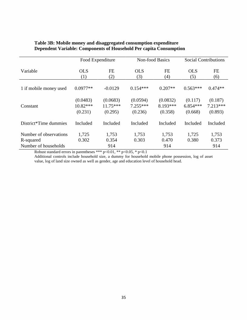
We further disaggregate our consumption expenditure measure into three categories –

expenditure on food items, non-food household basics and social contributions.7 Table 3B

gives a report of these three measures using both OLS and fixed effects estimations.

Column 1 shows that mobile money adoption has a positive impact on per capita food

expenditure, although the relationship disappears after controlling for unobserved time-

invariant household characteristics in Column 2. The average impact for basic expenditure

ranges between 15% and 20% for OLS and fixed effects models, respectively (Columns 3

and 4). Columns 5 and 6 reveal that a household that uses mobile money services

experiences between 47 and 56 percent higher value of social contributions. These results

should, however, be interpreted carefully, as they are likely to be capturing reverse

causality effects.8

Nonetheless, they suggest that social contributions and basic

expenditures respond more strongly to mobile money adoption as compared to food

expenditure. This result is not rather surprising, owing to the rural nature of households in

our sample which implies that a large fraction of consumed food comes from own farms.

Chetty and Looney (2006) argue that when consumption is close to subsistence level, any

shocks to income might not necessarily translate into reduced household consumption

because its level is already too low such that it cannot be reduced any further.

5.3 Mechanisms

5.3.1 Mobile money and household remittances.

7 Expenditure on household basics includes expenditure on school, medical, transport, clothing, cooking and

lighting materials. Social contributions cover expenses on ROSCAs, mutual support organizations – both

funeral and non-funeral, churches and mosques, other local organizations and credit repayments. 8 Household that make numerous social contributions may be convinced by members of their social networks

to join mobile money services for easier transmission of contributions.

19

As we predicted in earlier sections, the impact of mobile money on household welfare is

achieved through the facilitation of remittances. We explore into this claim by examining

whether households that have access to mobile money services have differential access to

remittances. These results are reported in table 4A. Being a mobile money user is

associated with a significantly higher probability of receiving remittances and the

remittances received are larger in number and total value compared with non-users. In

estimating the probability of a household receiving remittance, we estimate equation (4) as

a Probit model, since the dependent variable is binary. The results in Column1 show that

mobile money adoption increases the probability of receiving remittances by seven

percentage points. These results remain qualitatively unchanged when using OLS

regression in Column 2. In columns 3 through 6, we present the results from the other two

measures of remittances – number of remittances and total value received in the past 12

months. From Columns 3 and 4, mobile money users receive approximately one more

remittance at a given time, compared to non-users. The OLS estimates of total value of

remittances in Column 5 reveal that adopting mobile money services increases the total

value of remittance received by 36%. This translates into approximately 116,706 Uganda

Shillings (USD 61), as evaluated at the mean value of non-users. The fixed effects

estimation of remittance value in Column 6 yields similar results even after controlling for

unobserved time-invariant heterogeneity between users and non-users. In all specifications,

we include controls for household characteristics (mobile phone possession, household size,

asset value, land size, as well as age, education and gender of household head). The

20

inclusion of district-by-time effects in our regressions captures local macro trends that may

have differential influence on household access to remittances.

[Insert Table 4A here]

5.3.2 The influence of migration (job-seeking behavior)

We now account for the source of remittances and examine the possibility of differential

remittance structure between households that send their members to find jobs outside the

village in towns and those that do not. These results are reported in Table 4B. Column 1

reveals that, conditional on mobile money status and other covariates, households that send

their members to find town jobs are 11 percentage points more likely to receive remittances.

Columns 2 and 3 report results for the number and total value of remittances received,

respectively. Having a member working outside the village increases the number and total

value of remittances by 1.4 times and 42%, respectively. We believe that the introduction

of mobile money reduced the monetary and opportunity costs that hitherto hindered these

workers from transferring money to villages. Our presumption is that, even when members

were working in towns prior to the introduction of mobile money, the idiosyncratic lack of

a cheap and convenient money transfer mechanism rendered it hard for the members to

remit financial assistance back to their rural households. To check this claim, we perform

similar analysis on a sub-sample covering the period before mobile money inception in

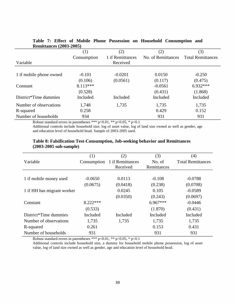
2009 – survey rounds of 2003 and 2005. The results in Table 8 suggest no significant

relationship between working outside the village and all measures of remittances and

21

consumption. The fact that this relationship emerged after mobile money establishment

provides partial evidence in support of impact of mobile money on remittances.

[Insert Table 4B here]

5.4 Results from Reduced Form Analysis

Table 5 reports the results from our reduced form analysis using log of distance to the

nearest mobile money booth as a measure of access to mobile money services at the

community level. The dependent variable in column 1 is the log of monthly household per

capita consumption. As earlier predicted, being located away from the mobile money booth

is associated with a significant reduction in household per capita consumption. The

probability, number and total value of remittances received, as measures of remittances, are

reported in columns 2, 3 and 4, respectively. Results are consistent with those reported in

our previous estimations. Households in located one kilometer away from the mobile

money booth have two percentage point lower probability of receiving remittances

(Column 2). Similarly, the frequency and total value of remittances received reduces

significantly with an increase in the distance to the mobile money agent. Note that the

treatment variable in this case is a community-level variable and the inclusion of district

and time dummies implies that our estimate is a conservative estimate of the true effect of

mobile money access as these controls absorb much of the variations in mobile money

access. Most importantly, controlling for district and time effects rules out the potentially

confounding effect of local access to services that tend to be concentrated in district towns.

22


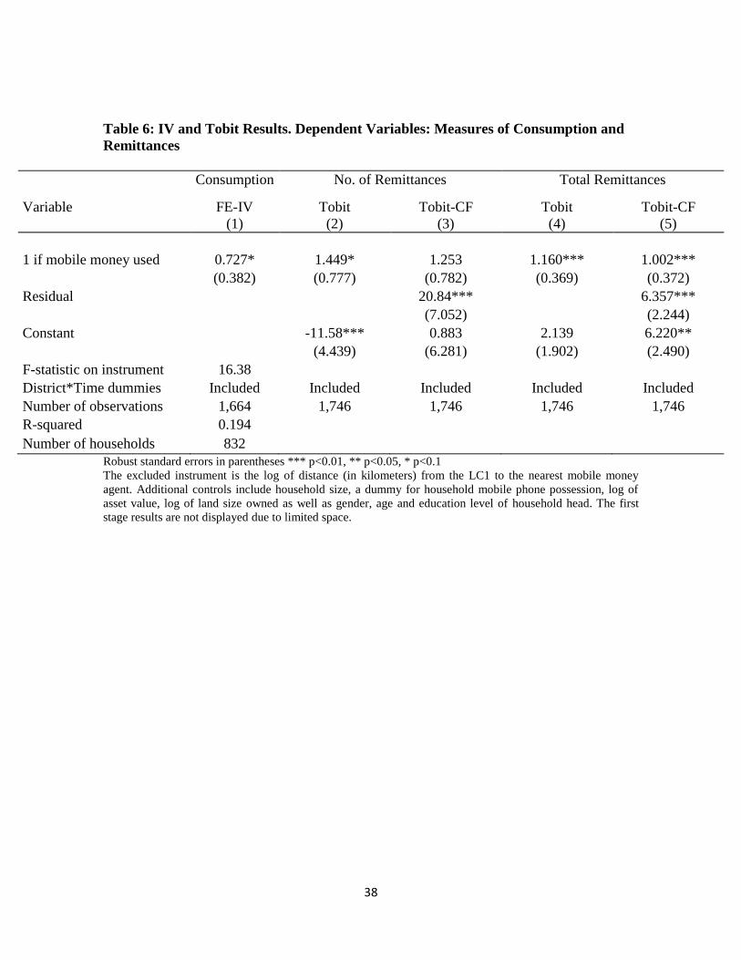
5.5 IV and Tobit Results

Results reported so far rely on the assumption that mobile money is not correlated with the

error term conditional on the other controls included in the regressions. However, where

this assumption does not hold, both OLS and fixed effects estimates may be biased. As

earlier noted, mobile money is potentially endogenous given reverse causality concerns –

households may adopt mobile money when they expect to receive remittances. In this

section, we account for this endogeneity using standard fixed effects IV method for

consumption and Tobit models with a control function approach for remittances. Apart

from capturing potential endogeneity, the latter technique takes into account the corner

solution problem resulting from the censored nature of our remittance variables, that is,

households that never received remittances have no observations for the number and total

value of remittances. In the control function version of our Tobit model, we include

residuals from the first stage estimation of the determinants of mobile money in the main

model. In both methods, we use log of distance to the nearest mobile money agent as an

excluded instrument for the potentially endogenous mobile money variable.

The results of these estimation methods are reported in Table 6. Column 1 reports

results of the consumption measure using standard fixed effects IV method. Columns 2

through 5 report the Tobit estimates of the number and total value of remittances received.

In columns 3 and 5, we combine Tobit with control function methods to control for corner

solution and endogeneity problems. Estimates in Column 1 reveal that per capita

23

consumption increases by 72 percent upon adoption of mobile money. Although we do not

show the first stage results for the IV regression because of space limitation, we report the

F-statistic on the instrument which shows that the instrument if valid. Columns 2 and 3

show that mobile money adoption approximately doubles the total value of remittances

received while Columns 4 and 5 show that users receive more than one additional

remittance relative to non-users. The number of remittances is positively associated with

mobile money usage, although the coefficient is not statistically distinguishable from zero

at conventional levels of significance. In line with Mason 2013, the significance of the

residual in Columns 3 and 5 not only implies potential endogeneity of the treatment

variable but also deals with the problem. We therefore focus on the results in Columns 3

and 5 for our measures of remittances.


5.6 Alternative Explanations

Local economic conditions at the village level could account for changes in mobile money

penetration and household per capita consumption. For example, mobile money agents

could locate in trading centers where economic activities are concentrated, while at the

same time business and employment opportunities near trading centers and towns could

provide alternative income sources that potentially increase consumption. Instrumenting

mobile money possession with distance to the nearest mobile money booth would

potentially capture the spurious positive relationship between mobile money and

24

consumption. We take two measures to address this concern. First, in all our regressions,

we control for the distance between the village center and the nearest district town where

major economic activities are concentrated to capture the local economic potential of the

corresponding villages. Secondly, since we use fixed effect IV (FE-IV) method withy time

and village dummies rather than the conventional IV framework, we smooth out

unobserved fixed attributes of the household as well as local time and village effects that

could potentially confound our results.

One might argue that the changes in remittance patterns could have resulted from

mobile phone possession which could have enabled rural households to contact their

members in towns in times of hardship. If this were the case, then mobile phone possession

would be expected to have a positive and significant effect on the flow of remittances

among the household members even in the absence of mobile money. In order to explore

into this possibility and thus disentangle any impact of mobile phone from that of mobile

money, we examined the relationship between mobile phone possession and household per

capita consumption and remittances prior to the introduction of mobile money. We

therefore run regressions of the outcome variables on a dummy variable of mobile phone

possession using 2003 and 2005 data, including a full set of controls as in previous sections.

As reflected in Table 7, there is no significant relationship between mobile phone

possession on one hand and consumption (Column 1) and remittances on the other

(Columns 2 through 5). At best, the remittance impact of mobile phone possession is

positive and statistically indistinguishable from zero. This partially rules out the possibility

25

that the observed consumption and remittance changes resulted majorly from mobile phone

possession.


6 Conclusion

Lack of access to financial services is a typical challenge to rural livelihood in many

developing countries. Apart from the direct hindrance on the ability to borrow and save, the

associated high costs of remitting funds to financially inaccessible areas impose a limit on

the effectiveness of informal sharing mechanisms among friends and relatives. Mobile

money - a new financial service that allows direct transaction via a mobile phone –serves to

bridge this gap given its relatively lower cost and convenience. In Uganda, mobile money

adoption has expanded tremendously over the past three years since its inception in 2009.

In this paper, we examine the welfare impact associated with this service by estimating its

impact on monthly household per capita consumption. Specifically, we provide evidence

that households using this financial innovation experience a significant increase in per

capita consumption. The result is robust to sensitivity checks, mainly the change in

empirical specification.

Disaggregating consumption into food, basic and social expenditures, we find

stronger impacts of mobile money for the social expenditure measure, partially suggesting

investment in informal social and insurance networks and saving mechanisms. There are a

26

number of potential pathways through which this result might be realized as cited in the

literature including the facilitation of savings (Jack and Suri, 2011) and self-insurance

through remittances. We provide evidence that the estimated impact is achieved through the

facilitation of remittances; households with access to mobile money services are more

likely to receive remittances, receive remittances more frequently and receive higher value

of remittances relative to non-users. Although we do not explicitly demonstrate due to data

limitations, we are convinced, based on anecdotal evidence that the average cost of

remitting funds across households reduced greatly with the event of mobile money

technology. We further venture into the role of family dynamics by comparing remittance

patterns across households with and without members working outside the village. We

provide a falsification test that the relationship between this migration measure and

remittances did not exist prior to mobile money, suggesting that its emergency after 2009

partially reflects reduction in transaction costs that made it possible for workers to remit

funds to their rural households.

The results presented in this paper suggest significant welfare benefits of access to

financial services which might go afield in reducing rural poverty through reduction in

vulnerability by the rural poor. Dercon (2006) suggests stronger welfare benefits of

informal insurance mechanisms if random reductions in consumption affect poverty

dynamics through persistent income reduction in incomes. One concern however is that,

although we plausibly assume reduction in remittance cost as the major pathway of the

welfare and remittance impact of mobile money, we do not test this premise within the

27

limitation of the data. This and the analysis of risk-sharing behavior will form the

foundation for further research.

28

References

Adger, W. N., Winkels, A. (2007). Vulnerability, poverty and sustaining well-being.

Handbook of sustainable development, 189.

Aker, J. C. (2010). Information from markets near and far: Mobile phones and agricultural

markets in Niger. American Economic Journal: Applied Economics, 46-59.

Aker, J. C., Boumnijel, R., McClelland, A., Tierney, N. (2011). Zap It to Me: The Short-

Term Impacts of a Mobile Cash Transfer Program. Center for Global Development

Working Paper, (268).

Becker, S., Hvide, H. (2013). Do entrepreneurs matter?. Unpublished Manuscript.

Buys, P., Dasgupta, S., Thomas, T. S., Wheeler, D. (2009). Determinants of a digital divide

in Sub-Saharan Africa: A spatial econometric analysis of cell phone coverage. World

Development, 37(9), 1494-1505.

Chavan, A. L., Arora, S., Kumar, A., Koppula, P. (2009). How mobile money can drive

financial inclusion for women at the Bottom of the Pyramid (BOP) in Indian urban

centers. In Internationalization, Design and Global Development (pp. 475-484).

Springer Berlin Heidelberg.

Chetty, R., Looney, A. (2006). Consumption smoothing and the welfare consequences of

social insurance in developing economies. Journal of Public Economics, 90(12), 2351-

2356.

Claessens, S. (2006). Access to financial services: A review of the issues and public policy

objectives. The World Bank Research Observer, 21(2), 207-240.

29

Combes, J. L., Ebeke, C. H., Etoundi, S. M. N., & Yogo, T. U. (2014). Are Remittances

and Foreign Aid a Hedge Against Food Price Shocks in Developing Countries?. World

Development, 54, 81-98.

Deaton, A., Zaidi, S. (2002). Guidelines for constructing consumption aggregates for

welfare analysis (No. 135). World Bank Publications.

Demirguc-Kunt, A., Klapper, L. (2012). Measuring Financial Inclusion: The Global

Findex.World Bank Policy Research Wp, 6025.

Dercon, S. (2006). Vulnerability: a micro perspective. Securing Development in an

Unstable World, 117-146.

Dercon, S., Gilligan, D. O., Hoddinott, J., Woldehanna, T. (2009). The impact of

agricultural extension and roads on poverty and consumption growth in fifteen

Ethiopian villages. American Journal of Agricultural Economics, 91(4), 1007-1021.

Donovan, K. (2012). Mobile money for financial inclusion. Information and

communication for development, 61-74.

Elul, R. (1995). Welfare effects of financial innovation in incomplete markets economies

with several consumption goods. Journal of Economic Theory, 65(1), 43-78.

Gilligan, D. O., Hoddinott, J., Taffesse, A. S. (2009). The impact of Ethiopia's Productive

Safety Net Programme and its linkages. The journal of development studies, 45(10),

1684-1706.

Gu, J. C., Lee, S. C., Suh, Y. H. (2009). Determinants of behavioral intention to mobile

banking. Expert Systems with Applications, 36(9), 11605-11616.

30

Heckman, J. J. (1979). Sample selection as a specification error. Econometrica: Journal of

the econometric society, 153-161.

Jack, W., Suri, T. (2011). Mobile money: the economics of M-PESA (No. w16721).

National Bureau of Economic Research.

Jack, W., Suri, T. (2011). Risk sharing and transaction costs: Evidence from Kenya’s

mobile money revolution’. Working paper.

Jack, W., Ray, A., Suri, T. (2013). Transaction Networks: Evidence from Mobile Money in

Kenya. American Economic Review, 103(3), 356-61.

Klein, M., Mayer, C. (2011). Mobile banking and financial inclusion: The regulatory

lessons (No.166). Working paper series//Frankfurt School of Finance & Management.

Marshall, J. N. (2004). Financial institutions in disadvantaged areas: a comparative analysis

of policies encouraging financial inclusion in Britain and the United

States. Environment and Planning A, 36(2), 241-262.

Mbiti, I., Weil, D. N. (2011). Mobile banking: The impact of M-Pesa in Kenya (No.

w17129). National Bureau of Economic Research.

Mohan, R. (2006). Economic Growth, Financial Deepening, and Financial Inclusion.

Muto, M., Yamano, T. (2009). The impact of mobile phone coverage expansion on market

participation: Panel data evidence from Uganda. World Development, 37(12), 1887-

1896.

31

Ndiwalana, A., Morawczynski, O., Popov, O. (2010). Mobile money use in Uganda: A

preliminary study. M4D 2010, 121.

Pousttchi, K., Schurig, M. (2004). Assessment of today's mobile banking applications from

the view of customer requirements. In System Sciences, 2004. Proceedings of the 37th

Annual Hawaii International Conference on (pp. 10-pp). IEEE.

32

Table 1: Summary Statistics by Year and Mobile Money Adoption Status

2009 2012

Non-Adopters Adopters Non-Adopters Adopters

VARIABLES Mean SD Mean SD Mean SD Mean SD

ICT Use

1 if mobile phone owned 0.5099 0.5003 0.5462 0.4985 0.6133 0.4874 0.9320 0.2520

1 if holds bank account - - 0.1269 0.3332 0.3815 0.4865

Wealth

Total value of assets (Ush) 266,466 564,907 411,356 568,729 390,208 555,563 831,826 1,189,717

Land holding size (acre) 5.7931 7.1484 7.1633 10.0797 5.5852 6.1938 6.9291 9.1896

Remittances

1 if received remittance 0.5036 0.5004 0.5098 0.5006 0.6558 0.4755 0.7892 0.4084

No. of Remittances 2.4116 4.7165 2.3838 4.6326 3.0394 5.0995 5.5496 7.3803

Total remittance (Ush) 566,222 1,002,502 558,571 914,789 621,833 1,116,481 1,088,673 1,595,953

Welfare

Per capita consumption (Ush) 27,484 28,121 31,488 25,073 43,524 35,182 54,636 41,080

HH Characteristics

Age of household head 53.1414 14.5252 53.3301 14.1900 52.6536 14.6563 52.7336 13.1949

1 if head is female 0.1170 0.3218 0.1481 0.3557 0.1554 0.3627 0.1569 0.3642

Head education 5.1611 3.6416 7.2138 4.1048 4.9328 3.5509 7.2215 3.9826

Household size 6.8675 3.2063 7.1512 3.6603 6.9068 3.4249 7.3549 3.6206

Village Characteristics

Distance to district town (km) 13.4557 10.9761 11.8712 9.5719 10.3639 8.4176 8.7333 7.5988

Number of households 521 325 521 325

Notes: Authors’ computation based on RePEAT 2009 and 2012. According to the annual Bank of Uganda

Report 2012, 1 USD was equivalent to Ush 2028 and 2557 in financial years 2008/2009 and 2011/2012,

respectively.

33

Table 2: Determinants of Household Mobile Money Adoption

(1) (2)

Variable Probit FE

1 if mobile phone owned 0.0806*** 0.117***

(0.0142) (0.0273)

1 if HH has migrant worker 0.0349*** 0.0908***

(0.0131) (0.0268)

Log of distance to nearest MM agent in km -0.0137*** -0.0442***

(0.00383) (0.0106)

HH head’s years of schooling 0.00543*** 0.0115***

(0.00152) (0.00332)

Head age 0.00192 0.00471

(0.00234) (0.00472)

Head age squared -1.50e-05 -4.16e-05

(2.17e-05) (4.32e-05)

Log of land size in acre 0.00207 0.00132

(0.00710) (0.0185)

Household size 0.000151 0.000378

(0.00135) (0.00365)

1 if head is female 0.0289 -0.0141

(0.0185) (0.0357)

Log value of total assets (UGX) 0.0195*** 0.0248**

(0.00485) (0.0114)

District*Time dummies Included Included

Number of observations 1,745 1,745

R-squared 0.448

Number of households 906 Robust standard errors in parentheses

*** p<0.01, ** p<0.05, * p<0.

34

Table 3A: Mobile money and Household Consumption

Dependent Variable: Household Per capita Consumption

(1) (2) (3)

Variable OLS FE FE

1 if mobile money used 0.135*** 0.110* 0.0947*

(0.0394) (0.0565) (0.0565)

Constant 9.144*** 8.611*** 9.359***

(0.288) (0.377) (0.383)

District*Time dummies

Included

Included

Number of observations

1,753

1,753

1,753

R-squared 0.300 0.272 0.379

Number of households 914 914

Robust standard errors in parentheses *** p<0.01, ** p<0.05, * p<0.1

Additional controls include household size, a dummy for household mobile phone possession, log of asset

value, log of land size owned as well as gender, age and education level of household head.

35

Table 3B: Mobile money and disaggregated consumption expenditure

Dependent Variable: Components of Household Per capita Consumption

Food Expenditure

Non-food Basics Social Contributions

Variable OLS

(1)

FE

(2)

OLS

(3)

FE

(4)

OLS

(5)

FE

(6)

1 if mobile money used 0.0977** -0.0129 0.154*** 0.207** 0.563*** 0.474**

(0.0483) (0.0683) (0.0594) (0.0832) (0.117) (0.187)

Constant 10.82*** 11.75*** 7.255*** 8.193*** 6.854*** 7.213***

(0.231) (0.295) (0.236) (0.358) (0.668) (0.893)


Included

Included

Included

Included

Included

Included

Number of observations

1,725

1,753

1,753

1,753

1,725

1,753

R-squared 0.302 0.354 0.303 0.470 0.380 0.373

Number of households 914 914 914




36

Table 4A: Mobile money and Household Remittances

Dependent Variable: Measures of Remittances

Dependent Variable: 1 if Remittances

Received

(1) (2)

No. of Remittances

(3) (4)

Total Remittances

(5) (6)

Variable Probit OLS OLS FE OLS FE

1 if mobile money used 0.0706* 0.0581* 0.843** 0.940* 0.360*** 0.381*

(0.0399) (0.0324) (0.421) (0.525) (0.133) (0.220)

Constant 0.0273 -5.028** -1.772 5.066*** 5.080***


(0.190)

Included

(2.441)

Included

(3.354)

Included

(0.872)

Included

(1.253)

Included

Number of observations 1,702 1,729 1,736 1,736 1,736 1,736

R-squared 0.228 0.188 0.261 0.278 0.286

Number of households 905 905 Robust standard errors in parentheses *** p<0.01, ** p<0.05, * p<0.1



Table 4B: Mobile Money, Job-seeking and Remittances. Dependent Variable:

Measures of Remittances

(1) (2) (3)

Variable 1 if Remittances

Received

Number of

Remittances

Total

Remittances

1 if mobile money used 0.0952** 1.385** 0.428***

(0.0456) (0.629) (0.163)

1 if HH has migrant worker 0.114*** 1.384*** 0.415***

(0.0327) (0.482) (0.138)

Constant 2.831 9.607***

(2.315) (0.605)

District*Time dummies Included Included Included

Number of observations 1,709 1,736 1,736

R-squared 0.265

Number of households 905 905 Robust standard errors in parentheses *** p<0.01, ** p<0.05, * p<0.1



37

Table 5: Reduced Form Results

(1) (2) (3) (4)

VARIABLES Consumption 1 if

Remittances

Received

No. of

Remittances

Total

Remittances

Log (distance to booth) -0.0481** -0.0211* -0.517*** -0.259**

(0.0238) (0.0127) (0.182) (0.123)

Constant 11.48*** 0.622*** 1.733 9.642***

(0.257) (0.141) (1.687) (1.104)

District*Time dummies Included Included Included Included

Number of observations 1,762 1,750 1,757 1,757

R-squared 0.345 0.216





38

Table 6: IV and Tobit Results. Dependent Variables: Measures of Consumption and

Remittances

Consumption No. of Remittances Total Remittances

Variable FE-IV

(1)

Tobit

(2)

Tobit-CF

(3)

Tobit

(4)

Tobit-CF

(5)

1 if mobile money used 0.727* 1.449* 1.253 1.160*** 1.002***

(0.382) (0.777) (0.782) (0.369) (0.372)

Residual 20.84*** 6.357***

(7.052) (2.244)

Constant -11.58*** 0.883 2.139 6.220**

(4.439) (6.281) (1.902) (2.490)

F-statistic on instrument 16.38

District*Time dummies Included Included Included Included Included

Number of observations 1,664 1,746 1,746 1,746 1,746

R-squared 0.194

Number of households 832


The excluded instrument is the log of distance (in kilometers) from the LC1 to the nearest mobile money

agent. Additional controls include household size, a dummy for household mobile phone possession, log of

asset value, log of land size owned as well as gender, age and education level of household head. The first

stage results are not displayed due to limited space.

39

Table 7: Effect of Mobile Phone Possession on Household Consumption and

Remittances (2003-2005)

(1) (2) (2) (3)

Variable

Consumption 1 if Remittances

Received

No. of Remittances Total Remittances

1 if mobile phone owned -0.101 -0.0201 0.0150 -0.250

(0.106) (0.0561) (0.117) (0.475)

Constant 8.113*** -0.0561 6.932***

(0.528) (0.431) (1.868)



R-squared 0.258 0.429 0.152



Additional controls include household size, log of asset value, log of land size owned as well as gender, age

and education level of household head. Sample of 2003-2005 used.

Table 8: Falsification Test-Consumption, Job-seeking behavior and Remittances

(2003-2005 sub-sample)

(1) (2) (3) (4)

Variable Consumption 1 if Remittances

Received

No. of

Remittances

Total Remittances

1 if mobile money used -0.0650 0.0113 -0.108 -0.0788

(0.0675) (0.0418) (0.238) (0.0708)

1 if HH has migrant worker 0.0245 0.105 -0.0589

(0.0350) (0.243) (0.0697)

Constant 8.222*** 6.967*** -0.0446

(0.533) (1.870) (0.431)



R-squared 0.261 0.153 0.431





mobile money, remittances and rural household welfare ... · 1 mobile money, remittances and rural...

Documents