mobile encounters: pattern analysis and profile embedding for

MOBILE ENCOUNTERS: PATTERN ANALYSIS AND PROFILE EMBEDDING FORMOBILE SOCIAL NETWORKING TESTBEDS

By

SUNGWOOK MOON

A DISSERTATION PRESENTED TO THE GRADUATE SCHOOLOF THE UNIVERSITY OF FLORIDA IN PARTIAL FULFILLMENT

OF THE REQUIREMENTS FOR THE DEGREE OFDOCTOR OF PHILOSOPHY

UNIVERSITY OF FLORIDA

2011

c⃝ 2011 Sungwook Moon

2

To Jin Yun, Dad, Mom, Kaylin Saeyun and my grandparents

3

ACKNOWLEDGMENTS

I sincerely thank to Dr. Ahmed Helmy for his excellent guidance for my Ph.D.

education. He is indeed a great research adviser and educator. I greatly appreciate for

his guidance. I also thank my supervisory committee for their valuable and encouraging

comments. I am truly grateful to my family. My wife, who shared all the great moments

and encouraged me to complete this education. It was a happy journey because I

shared this whole process with her. My parents who supported in every way that they

can possibly do. Just seeing my dad was a great education and motivation for me to

push myself harder. My mom’s countless supporting and caring words were always

big encouragement. My grandfather who was a role model and allowed me to dream

of becoming a great person. My daughter for making me smile and giving amazing

happiness. I appreciate my brother for giving me helps in many of computing techniques

and joy of sharing knowledges. NOMADS group members under Dr. Helmy helped

and supported me in great way as well. I particularly thank Udayan Kumar and Wei-jen

Hsu for sharing great technical and non-technical ideas that helped me to broaden my

experience and knowledge in so many things. I thank Yibin Wang on programming help

for Bluetooth scanning program and his idea of event based scenarios. I also thank

Gautam S. Thakur for many discussions and helps I received for research and defense

preparation. I thank Shao-cheng Wang and Sapon Tenachaiwiwat for their advice and

encouragement, and Jeeyoung Kim for review comments. It was a great opportunity for

me to learn so much from great individuals in NOMADs who not only are intelligent but

also have great personalities. I also thank all of my friends in CISE and South Korea.

Their support was very encouraging. The last but not the least, I thank God for allowing

me to experience such wonderful and valuable moments in my life and to finish the

education.

4

TABLE OF CONTENTS

page

ACKNOWLEDGMENTS . . . . . . . . . . . . . . . . . . . . . . . . . . . . . . . . . . 4

LIST OF TABLES . . . . . . . . . . . . . . . . . . . . . . . . . . . . . . . . . . . . . . 8

LIST OF FIGURES . . . . . . . . . . . . . . . . . . . . . . . . . . . . . . . . . . . . . 9

ABSTRACT . . . . . . . . . . . . . . . . . . . . . . . . . . . . . . . . . . . . . . . . . 11

CHAPTER

1 INTRODUCTION . . . . . . . . . . . . . . . . . . . . . . . . . . . . . . . . . . . 13

1.1 Research Framework . . . . . . . . . . . . . . . . . . . . . . . . . . . . . 131.2 Conceptual Model . . . . . . . . . . . . . . . . . . . . . . . . . . . . . . . 141.3 Mobile Networks . . . . . . . . . . . . . . . . . . . . . . . . . . . . . . . . 151.4 Problem Statements . . . . . . . . . . . . . . . . . . . . . . . . . . . . . . 16

1.4.1 Motivation and Challenge . . . . . . . . . . . . . . . . . . . . . . . 161.4.2 Problem Statements . . . . . . . . . . . . . . . . . . . . . . . . . . 171.4.3 Approaches . . . . . . . . . . . . . . . . . . . . . . . . . . . . . . . 17

1.5 Research Components . . . . . . . . . . . . . . . . . . . . . . . . . . . . 171.5.1 Analysis of Encounter Pattern . . . . . . . . . . . . . . . . . . . . . 181.5.2 Profiles of Mobile Nodes . . . . . . . . . . . . . . . . . . . . . . . . 191.5.3 Profile Based Mobile Social Networking Testbed . . . . . . . . . . 19

1.6 Contribution . . . . . . . . . . . . . . . . . . . . . . . . . . . . . . . . . . . 201.6.1 Effort Contribution . . . . . . . . . . . . . . . . . . . . . . . . . . . 201.6.2 Intellectual Contribution . . . . . . . . . . . . . . . . . . . . . . . . 20

2 RELATED WORK . . . . . . . . . . . . . . . . . . . . . . . . . . . . . . . . . . 21

2.1 Analysis of Encounter Pattern in Mobile Networks . . . . . . . . . . . . . 212.2 Mobile Social Networking Protocols . . . . . . . . . . . . . . . . . . . . . 222.3 Mobile Networking Testbeds . . . . . . . . . . . . . . . . . . . . . . . . . . 24

3 MOBILITY TRACES DATA . . . . . . . . . . . . . . . . . . . . . . . . . . . . . . 26

3.1 Basic Definitions . . . . . . . . . . . . . . . . . . . . . . . . . . . . . . . . 263.2 Network Traces . . . . . . . . . . . . . . . . . . . . . . . . . . . . . . . . . 263.3 Transforming Network Traces to Encounter Traces . . . . . . . . . . . . . 27

3.3.1 Bluetooth Encounter Traces . . . . . . . . . . . . . . . . . . . . . . 283.3.2 WLAN Traces . . . . . . . . . . . . . . . . . . . . . . . . . . . . . . 283.3.3 Transformed Encounter Trace . . . . . . . . . . . . . . . . . . . . . 30

4 UNDERSTANDING ENCOUNTER PATTERNS OF MOBILE NODES . . . . . . 31

4.1 Introduction . . . . . . . . . . . . . . . . . . . . . . . . . . . . . . . . . . . 314.2 Related work . . . . . . . . . . . . . . . . . . . . . . . . . . . . . . . . . . 32

5

4.3 Understanding Periodicity and Regularity of Mobile Nodes . . . . . . . . . 344.3.1 Methodology . . . . . . . . . . . . . . . . . . . . . . . . . . . . . . 344.3.2 Periodicities in Nodal Encounters . . . . . . . . . . . . . . . . . . . 37

4.3.2.1 WLAN trace . . . . . . . . . . . . . . . . . . . . . . . . . 374.3.2.2 Bluetooth trace . . . . . . . . . . . . . . . . . . . . . . . . 43

4.3.3 Periodicity of Individual Encounter Pattern . . . . . . . . . . . . . . 434.3.4 Regular Encounter . . . . . . . . . . . . . . . . . . . . . . . . . . . 47

4.3.4.1 Top frequency . . . . . . . . . . . . . . . . . . . . . . . . 474.3.4.2 Normalized regular encounter . . . . . . . . . . . . . . . 48

4.4 Temporal Stability of Mobile Encounter . . . . . . . . . . . . . . . . . . . . 504.4.1 Stability Window of Encounter History . . . . . . . . . . . . . . . . 514.4.2 Consistency of Encounter Pattern . . . . . . . . . . . . . . . . . . . 524.4.3 Application of Encounter Stability Analysis . . . . . . . . . . . . . . 554.4.4 Comparing Regular Encounter to Non-regular Encounter . . . . . . 56

4.5 Long-term Bluetooth Trace Analysis . . . . . . . . . . . . . . . . . . . . . 574.6 Conclusions and Future Work . . . . . . . . . . . . . . . . . . . . . . . . . 59

5 CAPTURING AND EMBEDDING PROFILES OF MOBILE NODES . . . . . . . 61

5.1 Introduction . . . . . . . . . . . . . . . . . . . . . . . . . . . . . . . . . . . 615.2 Related Work . . . . . . . . . . . . . . . . . . . . . . . . . . . . . . . . . . 625.3 Modeling Encounter Periodicity with Profile . . . . . . . . . . . . . . . . . 625.4 Discussion of Routing Based on Encounter Profiles . . . . . . . . . . . . . 645.5 Community Profiles of Mobile Users . . . . . . . . . . . . . . . . . . . . . 65

5.5.1 Location Visiting Preference . . . . . . . . . . . . . . . . . . . . . . 665.5.2 Encounter Vector . . . . . . . . . . . . . . . . . . . . . . . . . . . . 67

5.6 Conclusions and Future Work . . . . . . . . . . . . . . . . . . . . . . . . . 68

6 DESIGN OF A MOBILE SOCIAL NETWORKING TESTBED . . . . . . . . . . 71

6.1 Introduction . . . . . . . . . . . . . . . . . . . . . . . . . . . . . . . . . . . 716.2 Related Work . . . . . . . . . . . . . . . . . . . . . . . . . . . . . . . . . . 74

6.2.1 Analysis of Human Mobility . . . . . . . . . . . . . . . . . . . . . . 746.2.2 Mobile Networking Testbeds . . . . . . . . . . . . . . . . . . . . . . 756.2.3 Participatory Networks . . . . . . . . . . . . . . . . . . . . . . . . . 77

6.3 Testbed Architecture . . . . . . . . . . . . . . . . . . . . . . . . . . . . . . 786.3.1 Autonomous Mobile Nodes . . . . . . . . . . . . . . . . . . . . . . 786.3.2 Network of Autonomous Robots . . . . . . . . . . . . . . . . . . . . 796.3.3 Participatory Testing . . . . . . . . . . . . . . . . . . . . . . . . . . 806.3.4 Limitation of Controlled and Uncontrolled Environment . . . . . . . 82

6.4 Contact Rule-Based Decision Criteria . . . . . . . . . . . . . . . . . . . . 836.4.1 Power-law Distribution . . . . . . . . . . . . . . . . . . . . . . . . . 866.4.2 Memory . . . . . . . . . . . . . . . . . . . . . . . . . . . . . . . . . 87

6.5 Experiment . . . . . . . . . . . . . . . . . . . . . . . . . . . . . . . . . . . 876.5.1 Simulation Setup . . . . . . . . . . . . . . . . . . . . . . . . . . . . 87

6.5.1.1 Community profile . . . . . . . . . . . . . . . . . . . . . . 87

6

6.5.1.2 On-time scheduler . . . . . . . . . . . . . . . . . . . . . . 876.5.1.3 Environment setup . . . . . . . . . . . . . . . . . . . . . . 88

6.5.2 Experiment Modes . . . . . . . . . . . . . . . . . . . . . . . . . . . 896.5.3 Result Analysis . . . . . . . . . . . . . . . . . . . . . . . . . . . . . 90

6.5.3.1 Contact ratio with friends to strangers . . . . . . . . . . . 906.5.3.2 Rank group size . . . . . . . . . . . . . . . . . . . . . . . 916.5.3.3 Periodic contact pattern . . . . . . . . . . . . . . . . . . . 92

6.5.4 Visualization of Encounter and Mobility . . . . . . . . . . . . . . . . 936.6 Implementation on Autonomous Robots . . . . . . . . . . . . . . . . . . . 95

6.6.1 Controlling iRobot . . . . . . . . . . . . . . . . . . . . . . . . . . . . 956.6.2 Lab Environment . . . . . . . . . . . . . . . . . . . . . . . . . . . . 966.6.3 Evaluation Scenarios for Autonomous Robots . . . . . . . . . . . . 97

6.7 Conclusion and Future Work . . . . . . . . . . . . . . . . . . . . . . . . . 101

7 CONCLUSIONS . . . . . . . . . . . . . . . . . . . . . . . . . . . . . . . . . . . 102

7.1 Conclusions . . . . . . . . . . . . . . . . . . . . . . . . . . . . . . . . . . . 1027.2 Future Work . . . . . . . . . . . . . . . . . . . . . . . . . . . . . . . . . . . 103

REFERENCES . . . . . . . . . . . . . . . . . . . . . . . . . . . . . . . . . . . . . . . 105

BIOGRAPHICAL SKETCH . . . . . . . . . . . . . . . . . . . . . . . . . . . . . . . . 111

7

LIST OF TABLES

Table page

3-1 Statistics of encounter traces. . . . . . . . . . . . . . . . . . . . . . . . . . . . . 27

3-2 Format of WLAN traces . . . . . . . . . . . . . . . . . . . . . . . . . . . . . . . 29

3-3 Format of encounter trace . . . . . . . . . . . . . . . . . . . . . . . . . . . . . . 30

6-1 Properties in each node’s profile . . . . . . . . . . . . . . . . . . . . . . . . . . 87

6-2 Scheduler for on-time period . . . . . . . . . . . . . . . . . . . . . . . . . . . . 88

6-3 Scheduler for on-time duration . . . . . . . . . . . . . . . . . . . . . . . . . . . 88

6-4 Experiment environment . . . . . . . . . . . . . . . . . . . . . . . . . . . . . . . 88

6-5 Experiment modes . . . . . . . . . . . . . . . . . . . . . . . . . . . . . . . . . . 89

8

LIST OF FIGURES

Figure page

1-1 Framework of dissertation . . . . . . . . . . . . . . . . . . . . . . . . . . . . . . 14

4-1 Example encounter trace for a mobile user with one of the encountered nodes 35

4-2 Average autocorrelation coefficient . . . . . . . . . . . . . . . . . . . . . . . . . 36

4-3 Daily encounter: normalized frequency magnitude of frequency componentsfor encountered pairs . . . . . . . . . . . . . . . . . . . . . . . . . . . . . . . . 38

4-4 Encounter frequency: normalized frequency magnitude of frequency componentsfor encountered pairs . . . . . . . . . . . . . . . . . . . . . . . . . . . . . . . . 39

4-5 Encounter duration: normalized frequency magnitude of frequency componentsfor encountered pairs . . . . . . . . . . . . . . . . . . . . . . . . . . . . . . . . 40

4-6 Hourly encounter for Bluetooth pairs: frequency magnitude of frequency componentsfor hourly encounter at UF 08 spring/fall Bluetooth trace . . . . . . . . . . . . . 42

4-7 Daily encounter for individual nodes: normalized frequency magnitude of frequencycomponents for individual nodes’ encounter pattern . . . . . . . . . . . . . . . 44

4-8 Encounter frequency for individual nodes: normalized frequency magnitudeof frequency components for individual nodes’ encounter pattern . . . . . . . . 45

4-9 Encounter duration for individual nodes: normalized frequency magnitude offrequency components for individual nodes’ encounter pattern . . . . . . . . . 46

4-10 Empirical CDF of highest frequency for the encountered pairs at USC 06 springtrace according to daily encounter rate . . . . . . . . . . . . . . . . . . . . . . . 48

4-11 APs accessing preference at USC 06 spring trace . . . . . . . . . . . . . . . . 49

4-12 Ordered location visiting preference by encountered pairs according to dailyencounter rate . . . . . . . . . . . . . . . . . . . . . . . . . . . . . . . . . . . . 49

4-13 Window of encounter history . . . . . . . . . . . . . . . . . . . . . . . . . . . . 52

4-14 Average difference of the daily encounter rate at UF and USC campus accordingto the change of break point for the first window . . . . . . . . . . . . . . . . . . 53

4-15 Average difference of the daily encounter rate at UF and USC campus accordingto the change of break point for the second window . . . . . . . . . . . . . . . . 55

4-16 Average difference of the daily encounter rate at USC campus according tothe change of size for the first window of encounter history . . . . . . . . . . . 56

4-17 Time series data for the mobile user’s Bluetooth encounter . . . . . . . . . . . 58

9

4-18 Empirical CDF for each encounter metric with encountered nodes in the longterm Bluetooth trace . . . . . . . . . . . . . . . . . . . . . . . . . . . . . . . . . 59

4-19 Spectral analysis of long-term Bluetooth encounter . . . . . . . . . . . . . . . . 60

5-1 CDF of top 7 maximum frequencies . . . . . . . . . . . . . . . . . . . . . . . . 63

5-2 Overlay networks using periodicity as a link weight . . . . . . . . . . . . . . . . 65

5-3 Example of embedding profiles in various interfaces . . . . . . . . . . . . . . . 66

5-4 Location based association matrix for each mobile user (courtesy by Hsu [1]) . 67

5-5 Ranked size of groups for campus traces . . . . . . . . . . . . . . . . . . . . . 69

6-1 Bridging the gap between controlled and non-controlled environment . . . . . . 73

6-2 Picture of iRobot, its controlling Nokia N810 PDA and human carrying NokiaN810 PDA . . . . . . . . . . . . . . . . . . . . . . . . . . . . . . . . . . . . . . . 79

6-3 Communication structure among robots, personality interface, and communicationprotocol . . . . . . . . . . . . . . . . . . . . . . . . . . . . . . . . . . . . . . . . 81

6-4 State diagram of friend-stranger decision model . . . . . . . . . . . . . . . . . 84

6-5 Mobility of source node (Me) in each decision . . . . . . . . . . . . . . . . . . . 85

6-6 Visualization of simulation . . . . . . . . . . . . . . . . . . . . . . . . . . . . . . 90

6-7 Contact ratio of friends to strangers . . . . . . . . . . . . . . . . . . . . . . . . 91

6-8 Rank plot for group size in log-log scale in simulation . . . . . . . . . . . . . . . 92

6-9 Spectral analysis for contact with friends over 32 days in simulation . . . . . . . 93

6-10 Snapshots of simulation for each mode with visualization on. . . . . . . . . . . 94

6-11 Snapshot of a proof of concept video for mobile networking testbed . . . . . . 100

10

Abstract of Dissertation Presented to the Graduate Schoolof the University of Florida in Partial Fulfillment of theRequirements for the Degree of Doctor of Philosophy

MOBILE ENCOUNTERS: PATTERN ANALYSIS AND PROFILE EMBEDDING FORMOBILE SOCIAL NETWORKING TESTBEDS

By

Sungwook Moon

December 2011

Chair: Ahmed HelmyMajor: Computer Engineering

Study on human mobility is gaining increasing attention from the research

community for use in mobile networks. To better understand the potential of mobile

nodes as message relays, our study first investigates the encounter pattern of mobile

devices. Specifically, we examine extensive network traces that reflect mobility of

communication devices. We analyze the periodicity and consistency of encounter

patterns by using power spectral analysis. Our result shows the presence of strong

periodicity for rarely encountering mobile nodes and weak periodicity for frequently

encountering nodes. In addition, our investigation on the encounter history shows

that consistency depends on the encounter rate and length of history. With this

understanding of human encounter patterns, we discuss profiling of mobile users

based on their periodic properties in encounter pattern. In addition, we group mobile

users based on encounter days and discover that the rank group size follows power-law

distribution that we use in the assignments of communities for autonomous nodes.

To enhance the mobile networks testing, we utilize our findings to effectively capture

and embed personality of mobile users in simulation and testbed environment. We

propose an encounter rule-based decision to mimic human encounter pattern, which

is an important step toward efficient design of mobile social networking protocols and

services. With the additions of group information and scheduler to the rule-based

decision, we show that our approaches enable autonomous mobile nodes collectively

11

mimic human encounter patterns. We experiment with various types of decision modes

and compare the results to random mobility and real-world networking trace. The result

shows that our proposed approach provides the range of knobs for adjusting parameters

to capture power-law distribution of group sizes, encounter ratio with group members

and periodical encounter patterns that are close to real-world networking trace while far

outperforming random mobility. Finally, we propose a novel mobile networking testbed

that blends the network of autonomous robots and participatory testing via personality

profile. We implement a prototype mobile networking testbed with IRobot and PDAs.

12

CHAPTER 1INTRODUCTION

Research in this dissertation has three main components. The three main

components are: analysis of encounter patterns; capturing and embedding profiles

of mobile nodes; and designing of testbed for mobile networks with autonomous

mobile nodes. We first study the encounter pattern of mobile nodes to understand their

behavior in wireless networking. Specifically, we investigate periodicity and regularity

of the encounter patterns for mobile nodes. Then, we study the encounter history of

mobile nodes. Based on the results of the analysis, we introduce encounter based

profiling of mobile nodes using vectors and its use in encounter pattern modeling. With

the analysis and profile implementation of the encounter patterns, we develop mobile

testbeds using our proposed profiles for autonomous mobile nodes and discuss the

experiment results in simulation. Furthermore, we introduce a prototype implementation

of the mobile networking testbed with robots and PDAs. We conclude with our findings

and contributions of this dissertation.

1.1 Research Framework

We introduce our research framework in this section. Figure 1-1 shows an overview

diagram of our research works. The three square boxes in the top level shows the big

picture of each research work. Each research component has its own components.

The direction of arrow indicates the flow of the study. Arrow to the top indicates that the

small components make the big component. Whereas, down arrow indicates the small

components are the branches of the big component. We first introduce the study of

encounter pattern for mobile users. We analyze the network trace by periodicity, stability

and regularity. Based on our study on the understanding encounter pattern of mobile

nodes, the second component work has started. Specifically, we begin the study of

profiles in mobile nodes to utilize the result of analysis. We build an encounter vector for

each mobile user. We cluster the mobile nodes based on encounter vector and discover

13

Analysis of

Encounter

Patterns

Profiling Based

on Community

Embedding

Profile

Periodicity

Stability

Encounter

Vector

Network

of Robots

Participatory

Testing

Regularity

Cluster

Mobile

Networking

Testbed

Autonomous

Mobile Node

Simulation

Figure 1-1. Framework of dissertation. There are three main components: analysis ofencounter patterns, profiling based on community and embedding profile.The encounter pattern is analyzed with subcomponents of periodicity,regularity and stability. Profiling based on community study is performed bysubcomponent of encounter vector and encounter group size is analyzedusing the encounter vector for group size subcomponent. Profiles areembedded in the two subcomponents: autonomous mobile nodes andmobile networking testbed. Autonomous mobile nodes are simulated andimplemented in its subcomponents of simulation and network of robots.Mobile networking testbed component consists of two subcomponents thatare network of robots and participatory testing. Network of robots is aduplicate component as autonomous mobile nodes are used. Encountervector and participatory testing are mainly used to support othercomponents; thus, filled with a light color.

power-law distribution in the sizes of the groups. Then, we design and develop mobile

testbeds based on the profiling research.

1.2 Conceptual Model

We are living in a world where wireless LAN (WLAN) access is available in many

places, such as school, airport and coffee shop. Proliferation of mobile devices such

as smart phones and tablets demands more wireless networking areas. Advent of

popular smart phones such as iPhone and Android enables easy access to the internet

14

from mobile devices that people carry all the time. However, those mobile devices

are dependent on the infrastructure networks (i.e. wireless access point (AP) and

cell tower). Mobile adhoc networks allow the devices to communicate via wireless

communication when there are no such networking infrastructures available. Yet, they

can also be limited in the distance of communication where mobile devices are sparsely

deployed. Delay Tolerant Network (DTN) [2] is a networking concept that allows a

delay in communication between nodes. DTN can be many types of forms. For existing

networking infrastructure, there can be some links that are off but can be on again after

some time. For mobile networks where mobile nodes play a role of routers, the end

to end paths may exist when opportunity for communication comes in with mobility of

mobile nodes as they become relaying nodes. Consequently, with delays, the range of

wireless communication can be wider with the helps of mobile nodes forwarding data

or messages to the target nodes. We assume that mobile nodes can be relay nodes by

store and forward fashion. They become routers in a sense that they decide a next route

for the data packet and forward it to the next node or end node. In this dissertation, we

study the mobile networks where such concepts can be applied.

1.3 Mobile Networks

Mobile networks are networks that consist of mobile nodes that may roam around

and have wireless connectivity. Direct end-to-end path may not exist in such a network

but permission of delay makes the delivery possible as the new paths may become

available after certain delay. For instance, the new links can be opened when mobile

nodes get close to other nodes. Bluetooth communication (e.g., PDA, smartphone)

is an example of such new communication opportunity. Bluetooth communication,

however, is limited to direct communication. Unlike single hop networks, we assume

a network with multi-hop delivery capability as in existing infrastructure networks, only

the difference being a node can be both end node and relay node. This assumption

makes robust network against the malfunctions of several nodes and eliminates the

15

need of infrastructure; therefore, it is particularly useful in a situation like disaster relief

or military operation. Another upside of such networks is implicit multicast, which is

spreading a message to certain nodes of interest or groups based on their location

visiting preference. [3]

One of the main challenges in this network is unpredictable connectivity with an

exception of scheduled move, which is not our focus in this work. Our interest lies

in an environment where the most of carriers of the mobile devices are human. As

human mobility is unpredictable, so can be message delivery to the destination node. To

increase the prediction rate of connectivity among nodes in certain situations, significant

amount of recent researches have focused on social aspects of user mobility. Many

of these studies proposed a routing protocol that uses social characteristics of human

groups or mobility models to be used in simulation [3–5]. However, little is known about

the encounter pattern of mobile nodes, which is important in predicting next connectivity.

1.4 Problem Statements

We first discuss the motivation of our works along with challenges associated with

them. Then, we describe the problem statements. Explanation of our approaches in a

big picture are followed.

1.4.1 Motivation and Challenge

Motivations of our work are three folds: 1) understanding mobile users encounter

pattern, 2) discovering group encounter pattern of mobile users, and 3) designing a

mobile social networking testbed. For the first motivation of understanding mobile

users’ encounter pattern, it is crucial identifying specific dimension to explore. In

addition, domain knowledge obtained from analysis should be helpful in application of

understanding. The second motivation brings the challenges of define an appropriate

grouping vector and discovering similarity metric to cluster mobile users. The third

motivation has great challenges of designing and implementation of the testbed. To

create a realistic mobile testbed using human mobility, it is critical to use autonomous

16

mobile node that can make independent mobility decision by themselves like human

does. Deploying autonomous mobile nodes brings another challenge of emulating

human mobility pattern without global knowledge.

1.4.2 Problem Statements

To the motivations and challenges, we define our problem statements in four

categories: 1) identify periodic encounter pattern of mobile users; 2) discover encounter

patterns of mobile users using encounter based community; 3) design autonomous

mobile nodes collectively mimicking mobile users encounter pattern; and 4) propose

a novel idea to design a mobile social networking testbed and show a prototype

implementation.

1.4.3 Approaches

Our approaches to each problem statements are as follows. 1) Periodic encounter:

perform spectral analysis for WLAN and Bluetooth encounter traces that reflect

real-world human mobility. 2) Community encounter pattern: cluster mobile users

based on the similarities of encounter vector and embed as a community profile. 3)

Autonomous mobile nodes: embed encounter rule-based decision to the autonomous

mobile nodes along with scheduler and community profile. 4) Design a mobile social

networking testbed: implement a proof of concept on the robots and mobile devices

and develop a simulation tool for large-scale experiment while showing the mobility of

the nodes in graphics and validate the result by comparing to the real-world encounter

pattern appear from WLAN traces.

1.5 Research Components

In this section, we describe the main research components in detail. Each

component is tightly linked with strong relation to other components. We analyze

the encounter patterns first. Then, we propose the methods to capture mobile users’

behavior and create profiles based on them. We propose profile based mobile social

17

networking testbed utilizing analyzed encounter pattern of mobile users and profiling

methods.

1.5.1 Analysis of Encounter Pattern

We investigate the encounter patterns of mobile nodes and analyze their pattern

to apply to the human encounter model and message bundle protocol that uses the

encounter pattern. We use a lower bound metric to calculate the number of required

relay nodes for given success ratio condition. Advantage of this metric is that the source

node can determine the number of message copies according to the importance of

message without causing overload to the network. Then, we analyze the network traces

in various environments and show the presence of strong periodic patterns in nodal

encounter (a.k.a. periodic link connection), using spectral analysis. With this analysis,

we find the periodic patterns that are repetitive and discuss its application. To achieve

this goal of study, we analyze various types of Wireless LAN (WLAN) and Bluetooth

encounter traces. First, we generate encounter trace with an adequate assumption from

WLAN trace. Bluetooth trace is naturally an encounter trace without any transformation

as it recorded the Bluetooth devices identification each device actually encountered.

However, the scale of Bluetooth trace is limited; thus, we also use the processed

WLAN trace for encounter pattern analysis. In addition, we study the encounter history

of mobile nodes. Their encounter patterns can be either consistent or inconsistent

depending on the break point of the history. We divide the encounter history by two

different windows and analyze the consistency of encounter in both windows. Our

analysis result shows that as we have more encounter history data in the first window,

the overall consistency of encounter pattern improves. However, more history data did

not affect to the consistency of encounter pattern significantly. Further, we investigate

the encounter consistency by controlling the size of the second window. The result

shows that bigger second window size lowers the overall encounter consistency. With

these result of analysis, we design a encounter pattern model of mobile nodes that

18

reflects the metrics we found. We also provide a snapshot of the overlay networks with

the characteristics our analysis result shows.

1.5.2 Profiles of Mobile Nodes

With the analysis of mobile nodes, we aim to build profiles of mobile nodes by their

encounter pattern. Two types of profiles can be constructed. Firstly, the profile can be

built for aggregate encounter pattern for each node. Secondly, pair wise profiles can

be built for encounter with each node. The latter type of profiles can be heavier in size.

We focus on the second type of profile as it accurately depicts the encounter pattern

for each user. We cluster the mobile users based on the encounter vector we define

and analyze the trend. This encounter vector is the second type of profile that require N

number of columns, where N is the number of existing nodes. Based on the analyzed

trace, we reveal the distribution of cluster sizes, which is a basis in assignment of

communities in the mobile social networking testbed we discuss in the following section.

1.5.3 Profile Based Mobile Social Networking Testbed

Some of the mobile networking testbeds have been proposed in previous literatures.

The behaviors of mobile nodes, however, are limited to random mobility. To create

a realistic mobile networking testbed, it is imperative to use a behavioral model that

closely resembles human behavior. In order to achieve this goal, we use a concept of

encounter profile we discuss in the previous section. We embed the created profiles

on the robot to build a testbed that emulates the behavior of human. By implementing

the profiles on the robots, we have freedom of controlling the profiles, yet, we also

have advantage of emulate human mobility on the testbeds. However, scalability of

the networks are still limited to the number of mobile nodes created in the lab. For

instance, using mobile robots costs significantly high if purchased more than hundreds.

For successful deployment of mobile networking, it is essential to have large number of

nodes for networking purpose. We adopt a concept of participatory testing to improve

the scalability. With this approach, voluntary human participants carrying smart phones

19

become test subjects. This creates a huge testbed as the size of the testbed can be

as large as the number of participants. Efficient recruiting strategy is a key in drawing

more participants. However, it is out of scope of this dissertation; thus, our focus is on

proposing the realistic testbeds, evaluating the testbed via simulation and showing the

prototype of the testbeds. Our testbeds provide the controllable profiles that reflect

human behavior with scalability by crowd sourcing.

1.6 Contribution

Our contributions include two areas: effort contribution and intellectual contribution.

1.6.1 Effort Contribution

1) We build a trace library and process the traces for the purpose of encounter

pattern analysis. 2) We develop a simulation tool to visualize the encounter pattern of

mobile nodes and generate encounter statistics for encounter vector and time-series

data. 3) We build a prototype mobile testbed for proof of concept, where we embed an

emulation profile on robot nodes to mimic human encounter pattern. 4) We evaluate

the autonomous mobile nodes for community encounter pattern, group distribution and

periodic encounter pattern with various encounter metrics of encounter days, frequency

and duration via simulation.

1.6.2 Intellectual Contribution

1) Our finding from periodicity analysis provides insight into the periodical nature

of encounter pattern for mobile users. 2) We define encounter vector and discover

power-law distribution of mobile encounter clusters. 3) We propose a encounter

rule-based decision for autonomous mobile nodes which collectively emulate community

encounter pattern found from the networking traces.

20

CHAPTER 2RELATED WORK

We discuss related research works in the literature. We first introduce the other

research works that uses related definitions, assumptions and network environments.

In addition, we discuss the projects and literatures that include the data sets we use.

We further discuss the research works that study the mobile networking by describing

the relevant studies of analysis of mobile nodes, modeling and protocols in mobile

networking. We introduce the related testbeds projects and literatures of mobile

networks as well.

2.1 Analysis of Encounter Pattern in Mobile Networks

The advent of Delay Tolerant Networks (DTN) makes the mobile adhoc networks

to have broader concept of networks. With its mobility characteristics in mobile

adhoc networks, mobile networks become available without existing infrastructure.

Allowance of delay encompasses the mobile adhoc networks not only to larger spatial

communication space but also to longer temporal communication space. With similar

definition of DTN, intermittent connectivity and opportunistic networks also play the

same role; thus, these are the basis of the networks environment we study. Pocket

Switched Network [6] is a network where communication is performed among only the

mobile devices. This is also a similar environment with our focus of study; however,

Pocket Switched Networks differs in that it is for only among the mobile devices carried

by human. Whereas, the networks of study in this dissertation includes the statistic

networks such as network infrastructures.

[7] analyze the network traffic and revealed the presence of combination of

periodicity in the case of denial of service attacks on the internet. They apply power

spectral analysis that applies ACF to the time series data before transforming to

frequency domain. This removes sync terms that might appear for a finite set, therefore,

we adapted a similar approach rather than applying DFT to the data sets directly. Kim

21

et al. study the periodic properties of WLAN users association with access points [8].

They measure the diameter of visited APs for highly mobile users whose maximum

diameter within an hour is 100 meter or more from the Dartmouth campus WLAN data.

The result shows the strong presence of periodicity of diameter, particularly 24 hour

and 1 week, for the selected 360 users. Periodic properties of travel distance for highly

mobile users are interesting findings. This is the closet work to our frequency analysis in

that it uses DFT (Discrete Fourier Transform) to analyze the periodicity of user mobility.

However, we investigate the different aspect of user mobility pattern, namely, their

encounter pattern. Further, ACF (Auto Correlation Function) is used before applying

DFT to remove sync terms that might appear for a finite set; additionally, we analyze the

rich data set, including over 10,000 users per WLAN trace and Bluetooth trace.

2.2 Mobile Social Networking Protocols

Many of the studies in mobile networks were devoted in routing. Specifically,

large portion of mobile networks routing study focused on using human mobility for

routing messages and data. The main characteristics used in mobile networks routing

from social networks are community, mobility and encounter of human. To use such

characteristics in routing, deep understanding of human behavior is essential. Gonzalez

et al. [9] has shown that individual human tends to follow simple reproducible patterns

based on the cell phone user traces. Hsu et al. proposed time-variant community model

[10] that reflects the periodic encounters. Community structure of social networks from

networking traces are discussed in [11]. Social relationship between mobile nodes

for DTN routing is discussed in [4] [5]. Miklas et al. [12] divided human encounters

to friends and strangers according to the length of encounter. These works study

human encounter pattern; however, we are the first to analyze the periodicity of human

encounter extensively by spectral analysis. Prophet [13] is one of the first routing

algorithms using encounter history in DTN [2]. It uses encounter frequency to determine

a relay node. The chosen node will forward the message bundle to the encountered

22

node and delegate the responsibility of delivery to the node if the node has higher

encounter frequency to the destination node. However, it is unclear how to determine

the probability of encounter using frequency. To use encounter frequency for probability,

total number of possible encounters should be known, which otherwise could be infinite.

Further, it is possible that frequent encounters in short time can mislead prediction

of future encounter. Timely-count probability [14] is an idea that regards encounters

belonging to the same interval as one encounter; thus, it provides standard procedure to

calculate the encounter probability. In our work, we used it for an idea of daily encounter

whose interval is a day. Our analysis part of the study in this dissertation can be the

basis to improve the performance of protocols in DTN. Profile-cast [3] is a forwarding

protocol to the group of nodes, sharing the same interest. It has two ways in message

distribution: 1) source node propagates the message to the node with similar profile

to the destination group, which may also forward to other nodes that are more similar

(gradient ascending); 2) the source node can try to distribute the message to the nodes

that have different profiles, such that its different mobility can give more chance to reach

the destination group. Both profile-cast and prophet protocols can enhance their stability

of delivery by incorporating periodic properties of encounter for consistent predictability.

Studies for predictability of human mobility and encounter [15] [16] can also be extended

by considering different periodic properties as well as worm propagation pattern via

human encounter [17] [18].

Recent studies show the applications of using human mobility and encounter

for message propagation [19] [13] [20] [21] [22]. MobiTrade [22] is implemented on

Android phones for sharing the data with incentive. Human mobility in theme park is

implemented on message delivery in [19]. Popularity of locations is shown to influence

routing decision for efficient delivery of message using human mobility [21].

23

2.3 Mobile Networking Testbeds

There are research projects to design and develop mobile networking testbeds. We

explain the testbeds that are related to our works. MiNT [23] is a miniaturized network

testbed that solely uses iRobots in a controlled space. A server computer controls

the movements and communication amongst iRobots that are equipped with WLAN.

Although this testbed can expand with multiple numbers of iRobots and be effective

in experiments for small-scale mobile adhoc networks, it still suffers from scalability

and a diversity of nodes. Roomba MADNeT [24] showed the capability of using iRobot

for DTN. The researchers mounted a wireless router that runs on Linux by connecting

through modified serial cable. This process might take advantage of a costumed

lightweight programming board to utilize the wireless communication feature specifically

for the testing purpose. However, this process can be tedious and cumbersome to

many researchers who are not skilled in this area. Our method is simple and uses the

existing device. Connection requires a minimum of steps and effort: either Bluetooth

pairing or connecting a serial cable directly with a distant or attached computer. In

[25], the authors proposed a DTN testbed. They used enclosures to contain the laptop

computers and measure the signal attenuation for implemented DTN protocol. The

design is centralized and users can view the wireless nodes moving around from the

server computer. Mobility is limited to a controlled environment, as the participants are

to follow the given paths and required to be in the experiment range. Mobile Emulab [26]

is wireless sensor networks testbed that manages its MiCa2 mote based robot nodes

from a central computer with video camera. GUI interface provides location precision of

1cm for moving robot nodes.

In our presentation, nodes can have complete control of their movements, including

message propagation decisions. Moreover, measurements are decentralized in our

experiment, as each measurement record is kept inside the mobile nodes. SCORPION

[27] is a heterogeneous networking testbed, which uses iRobots, Buses, Aircrafts and

24

humans with briefcase nodes. It provides a testbed to experiment communication

between diverse movements; however, mobility of all the mobile nodes are limited to

controlled movements; thus, social aspects are not reflected. Our unique contribution

comes from the autonomous robots with behavioral profiles and participatory humans

that provides uncontrolled, thus, realistic testing environment.

25

CHAPTER 3MOBILITY TRACES DATA

It is crucial to have extensive and realistic data sets for the analysis of mobility. We

introduce the data sets we used and collected for our analysis along with definitions and

assumptions. In addition, we describe the details of transforming the network data sets

into the encounter traces for our analysis.

3.1 Basic Definitions

Before we explain the network traces, we first describe the basic terminologies that

we use in our work. Mobile node is an entity that can move around with different speeds

in different time and space. Mobile node is capable of wireless communication. Mobile

nodes can encounter each other when they are close enough to discover each other.

Specifically, the term encounter in this work indicates the event that two or more mobile

nodes present within the wireless communication range. The terms, encounter and

contact, are used interchangeably in literatures [1] [28] and we use the term encounter

throughout the paper for consistency. Mobile nodes have on-line and off-line behaviors.

In off-line mode, other nodes may not discover the mobile nodes even if they are in

the proximity of wireless communication range. These mobile nodes can be the smart

phones or PDAs human carry around or wireless communication devices that move

around or stay in static locations.

3.2 Network Traces

For accurate analysis of encounter patterns for mobile nodes, it is essential to have

large data sets. There are two types of a contact trace. First approach is obtaining

a trace by the synthetic trace. The synthetic trace is a artificially made trace based

on mobility model. The advantage of using such trace is freedom of manipulating the

data to fit the purpose of analysis. However, the synthetic trace is limited in that it is

based on the assumptions and observed parameters from previous analysis; thus, its

closeness to reality depends on the quality and quantity of samples used in analysis

26

Table 3-1. Statistics of encounter traces.Trace Trace Analyzed Unique users Encounter pairssource duration durationUSC 2006 Jan-May 128 days 28,173 25,359,454

2007 Jan-May 35,274 19,057,0892008 Jan-May 42,587 31,289,100

UF 2007 Aug-Dec 128 days 46,115 12,493,4032008 Jan-May 50,549 16,807,427

Monteral 2004 Aug-Dec 128 days 455 2,512Bluetooth 2/25 - 3/7/2008 256 hours 10 1,277

11/17-27/2008 27 1,655Long-term Bluetooth 2010/9-2011/4 180 days 1 27,870

for the model. Second approach is using a real world trace. The real world trace can

be divided into the trace by the mobile robots, human mobility and hybrid of both. By

using the robots, researchers can control the mobility of each robot for the purpose

of their experiments. This is similar to the synthetic trace but it differs in that it can be

experimented in real world environment as opposed to artificial environment in synthetic

trace. Collecting human contact pattern is limited in size to the participants willing to

follow the instructions.

Table 3-1 shows the traces we use in our analysis. Privacy issues of the traces are

out of scope of this dissertation. Interested readers regarding the anonymity of traces

and privacy issues are encouraged to read [29] [30] [31] [32] [33]. The WLAN traces

are publicly available for download at [34] [35]. Bluetooth traces are obtained by class

students and obtained with consent by participants for research purpose.

3.3 Transforming Network Traces to Encounter Traces

We use the two types of data sets for nodal encounter: Bluetooth traces and WLAN

traces. Bluetooth traces reflect the encounters of users carrying mobile devices with

Bluetooth communication capabilities. The limitation of Bluetooth traces is the scalability,

because the data set is limited to the number of participants willing to run the Bluetooth

discovery program. Whereas, WLAN traces can be very large as the centralized

system can continuously collect the data via access points belonging to the particular

27

organization (e.g., college campus). As discussed earlier, we use an assumption that

the users who accessed to the same access points (APs) have encounter events. This

assumption may not reflect the exact encounter; however, it is close to real encounter

considering the users accessed the same APs were at the close proximity of each other

and could have communicated each other through the AP.

3.3.1 Bluetooth Encounter Traces

Scale of Bluetooth encounter data is considerably small, compared to WLAN traces

due to the difficulty of finding subjects to participate. Some of the available Bluetooth

encounter data include the conference encounter [36] and bus encounter [37] [38].

While these data sets may be useful for particular scenarios, we conducted our own

experiment to observe general Bluetooth encounter, which matches to the WLAN trace

we also collect. Each of graduate students taking the Computer Networking course in

2008 was assigned a PDA (HP iPAQ or Nokia N800/810) and was strongly encouraged

to carry the mobile device as often as possible with the Bluetooth encounter collection

program running. This program broadcasts the beacon signal every 60 seconds and

logs the Bluetooth device information that acknowledges the beacon signal, including

the time stamp. This experiment was performed for two semesters (2008 spring and fall)

[35], each with different groups of students. Due to the short length of experiment, we

observed hourly encounter instead of daily encounter. As Table 3-1 shows, there are

10 and 27 subjects in spring semester and fall semester respectively. These collected

Bluetooth traces contain the information of the encountered nodes, namely their MAC

addresses and timestamps for acknowledgements.

3.3.2 WLAN Traces

There are many forms of network traces available in public, which can be obtained

from [34], including the city of Montreal trace [34] that we use in this paper. To obtain

large scale network traces that cover the entire campus over a length of more than

one academic semester, we collected campus-wide WLAN traces at the University of

28

Table 3-2. Format of WLAN tracesMAC Access Point Time stamp Duration of Associationab-cd-34-4d-23-12 lbw343-win-ap1200-1 1201889300 34003a-3d-4f-fe-ca-b8 lbw343-win-ap1200-1 1201889474 1200

Florida (UF, 2007 fall - 2008 spring semester) [35]. We also used the WLAN traces of

the University of Southern California (USC, 2006-2009 spring semesters) [35] as in Fig.

3-1. These WLAN traces have the following information - MAC address, associated

AP and timestamp for start and end time of association. Based on the assumption

described earlier, the WLAN traces are processed to encounter traces that log the MAC

addresses of the encountered WLAN devices, timestamps, durations and locations of

encounter. Conversion to the encounter trace is computation and storage consuming

process. Given m inputs in average for n number of nodes, the computation needed isn(n−1)

2∗m2 as it requires the comparison for each input between two nodes to determine

the occurrence of encounter and its duration. Therefore, we obtain O(n2m2) for overall

computation time in generating encounter trace and O(n2m) for the size of encounter

trace data. If the orignal trace is sorted in time sequence, the computation reduces

to O(n2m) because the comparison for the inputs of two nodes can be performed in

sequence of proceeding time. For the size of very large data, which has at least over

28,000 nodes with the inputs ranging up to several megabytes for a monthly data, it is

realistic to break down the entire trace by the certain periods for analysis purpose. We

analyze the 128 days of data from each trace for the above reasons and consistency in

comparison. Further, this specific time span roughly covers the entire semester for both

campuses.

Original format of WLAN trace contains much information. To generate encounter

trace we only need to use ID of an user, his association time with access points and

the ID of access points. Therefore, we process the trace to simple format that contains

only the necessary information as shown in figure 3-2. User ID is identified by the MAC

address their mobile devices has. Time stamp is the time a user starts to access the

29

Table 3-3. Format of encounter traceSource MAC Encountered MAC Time stamp Encounter durationab-cd-34-4d-23-12 3a-3d-4f-fe-ca-b8 1201889474 1200

WLAN access point. Each access point has unique identifier that sometimes change

after a semester is over. Thus, we investigate each semester separately. Number of

access points also increases over time as well. USC trace contains around 200 APs and

UF trace contains over 500 APs. Duration of association is the time a user spends at

certain APs.

3.3.3 Transformed Encounter Trace

Table 3-3 shows the transformed encounter trace. This format applies to the

Bluetooth trace as well, which does not require transformation. Based on the timestamp

and AP that duplicate between two mobile nodes, we build an encounter trace with

source MAC and encountered MAC. This transformed trace is the trace we use in this

dissertation.

30

CHAPTER 4UNDERSTANDING ENCOUNTER PATTERNS OF MOBILE NODES

It is essential to understand the encounter patterns of mobiles nodes for any of

the protocols using mobile nodes as forwarding nodes. We analyze the periodicity of

mobile nodes and propose heuristic approaches to find regularly encountering pairs.

Furthermore, we study the encounter history of mobile nodes. This analysis is the

critical basis for designing an encounter patten model for mobile networking protocols

and services.

4.1 Introduction

Mobility and nodal encounters are utilized to deliver messages in intermittently

connected delay tolerant networks (DTNs) [2]. Much of DTN research so far has been

devoted to the study of message delivery protocols and the design of mobility models.

While these studies are essential for eventual implementation of the mobile adhoc

networks using DTN concept, understanding of nodal encounter pattern is a critical

basis for the success of protocol deployment as delivery mechanism depends on nodal

encounter. In this presentation, we explore the periodicity presences in encounter

patterns and analyze them. By the spectral analysis of encounter pattern, we find the

periodic patterns that are repetitive and discuss their applications later. To achieve this

goal of study, we analyzed various types of the Wireless LAN (WLAN) and Bluetooth

encounter traces. First, we generate the encounter traces with a reasonable assumption

from WLAN traces. Bluetooth traces are naturally encounter traces without the need of

any transformation as they log the identification of the Bluetooth device that the subject

Bluetooth devices have discovered. However, the scale of Bluetooth traces are limited

to the number of subjects carrying the devcies with the discover program on. Hence,

we use the WLAN traces for scalable analysis of encounter pattern. In order to use

the WLAN trace as encounter trace, we use common assumption that had been used

by other publications [1] [39], which defines the encounter occurrence in the WLAN

31

environment as the nodes that are associated with the same access points (APs) in

the same period of time. After transformation to the encounter trace, the next step is

generating a time series data for the number of metrics, namely, daily/hourly encounter,

encounter frequency and encounter duration. We apply the Auto Correlation Function

(ACF) to identify the repetitive patterns and perform power spectral analysis to find

the distinct periodicities in encounter patterns for each metric. Fast Fourier Transform

(FFT) was performed in conversion to frequency domain for computation efficiency

and analyzes the frequency magnitude in the spectrum. We highlight the important

periodicities by different groups and discuss the utilization of the result in the mobile

networks. After analyzing the periodicity, we show some of approaches to extract the

periodically encountering node pairs and conclude with the summary and applications.

In the following section, we introduce the methodology to analyze the periodicity

along with the encounter traces in section II. Analysis of periodicity for the encountered

pairs and individual encounter patterns in WLAN and Bluetooth traces follow in section

III. Then, section IV describes the approaches to extract regularly encountering node

pairs and discuss the results. We explain about related works in section V, and wrap up

with conclusions and summary in section VI.

4.2 Related work

Many of studies on DTN/opportunistic/intermittent connectivity routing were devoted

in using the social aspects of networks, such as community, mobility and encounter.

Gonzalez et al. [9] has shown that individual human tends to follow simple reproducible

patterns based on the cell phone user traces. Hsu et al. proposed time-variant

community model [10] that reflects the periodic encounters. Social relationship between

mobile nodes were discussed for DTN routing in [4] [5]. Miklas et al. [12] divided human

encounters to friends and strangers according to the length of encounter. These works

study human encounter pattern; however, we are the first to analyze the periodicity

of human encounter extensively by spectral analysis. Prophet [13] is one of the first

32

routing algorithms using encounter history in DTN [2]. It uses encounter frequency

to determine a relay node. The chosen node will forward the message bundle to the

encountered node and delegate the responsibility of delivery to the node if the node

has higher encounter frequency to the destination node. However, it is unclear how to

determine the probability of encounter using frequency. To use encounter frequency for

probability, total number of possible encounters should be known, which otherwise could

be infinite. Further, it is possible that frequent encounters in short time can mislead

prediction of future encounter. Timely-count probability [14] is an idea that regards

encounters belonging to the same interval as one encounter; thus, it provides standard

procedure to calculate the encounter probability. In our work, we used it for an idea of

daily encounter whose interval is a day. Our periodicity and regularity analysis can be

the basis to improve the performance of protocols in DTN. Profile-cast [3] is a forwarding

protocol to the group of nodes, sharing the same interest. Both profile-cast and prophet

protocols can enhance their stability of delivery by incorporating periodic properties of

encounter for consistent predictability. Studies for predictability of human mobility and

encounter [15] [16] can also be extended by considering different periodic properties as

well as worm propagation pattern via human encounter [17] [18]. [8] studied the periodic

properties of WLAN users association with access points. They measured the diameter

of visited APs for highly mobile users whose maximum diameter within an hour is 100

meters or more from the Dartmouth campus WLAN data. The result showed strong

presence of periodicity of diameter, particularly 24 hours for the selected 360 users. This

is the closest work to our frequency analysis in that it uses DFT on the time series data

to analyze the periodicity of user mobility. [7] analyzed the network traffic and revealed

the presence of combination of periodicity in the case of denial of service attacks on the

internet. They applied power spectral analysis that applies ACF to the time series data

before transforming to frequency domain. This removes sync terms that might appear

33

for a finite set, therefore, we adapted a similar approach rather than applying DFT to the

data sets directly.

4.3 Understanding Periodicity and Regularity of Mobile Nodes

We discuss the methodology and analysis results in this section.

4.3.1 Methodology

For spectral analysis of the encounter traces, multiple steps are required. In our

work, raw network traces are processed to the encounter traces in the form of time

series data. We apply the autocorrelation function (ACF), and then transform them

to the frequency domain by performing the discrete-time Fourier transform (DFT). To

capture the multiple aspects of encounter behavior, we look into the following variables:

encounter frequency Fd(i , j), daily encounter Ed(i , j), houly encounter Eh(i , j) and

duration of encounter Ld(i , j), where given n number of nodes, (i , j) is the encountered

node i and j(0 ≤ i < n, 0 ≤ j < n, i ̸= j) and d is a day (0 ≤ d < T ), where

T is a total length of trace in days. Daily Encounter is a binary process. For each

encounter pair of nodes i and j on day d, Ed(i , j) = 1 if at least one encounter event

occurs in day d ; otherwise, Ed(i , j) = 0. Hourly encounter is the same process as the

daily encounter except the time unit is an hour. Daily and hourly encounter are interval

counting with an interval being a day and an hour respectively. We adapt this idea of

timely-counting [14]. Encounter Frequency is number of encounters a day and denoted

by Fd(i , j) = µ, where µ is the total number of encounter events occurred in day d and

0 ≤ Fd(i , j) < 24 ∗ 60 ∗ 60. Encounter duration is another metric used and denoted by

Ld(i , j) = ξ, where ξ is the total duration of encounter event occurred in seconds in day i

and 0 ≤ Td(i , j) < 24∗60∗60. The result periodicity patterns for the encounter frequency

and duration appear very similar to the patterns in daily encounter; thus, analysis and

observances for these two metrics are identical.

In both of the encounter traces, the timestamps log in seconds. To better observe

the daily and hourly encounter characteristics, we process the trace data in days and in

34

0

1

d (days)1285 21 54 72

Ed(i,j)Encounter ! Encounter ! Encounter !

51 109

Figure 4-1. Example encounter trace for a mobile user with one of the encounterednodes

hours, respectively. As noted earlier, 128 days are the time spans for each of the trace

in this analysis. This time spans are also beneficial to the use of Fast Fourier Transform

(FFT) in frequency analysis because it requires the length of data to be the power of

two. Applying FFT for each semester data enables fast processing of massive encounter

data and helps observing distinct characteristics in a finer granularity by preventing the

seasonal effect (repeated behavior by each semester) from affecting the result.

Figure 4-1 shows an example encounter trace of a mobile user and its encounter

history with one of the encountered nodes for daily encounter metric, Ed(i , j). In the

figure, boxed period is the days the two nodes encountered each other, thus, setting

a value of one for Ed(i , j). Each user has a number of such traces depending on the

number of encountered nodes.

ACF is a measure of correlation between observations at different lags (distances)

apart [40], thus providing insight into the stream of data. We use ACF to find the

repetitive periodical patterns from the processed time-domain representation of

encounter traces. When lag k = 0, it compares the data stream to itself, and

autocorrelation is maximum, which results in Variance(δ). Given the mean λ of a pair

(i , j), we calculate autocorrelation coefficients (autocoefficients) for the pair, rk(i , j) for

each lag k(1 ≤ k < T ), by computing the series of autocoefficients as in the following:

rk(i , j) =

∑T−k

d=0 (Ed − λ)(Ed+k − λ)∑T−1d=0 (Ed − λ)2

(4–1)

35

0 20 40 60 80 100 120 140−5

0

5

10

15x 10

−3

lag

auto

corr

elat

ion

coef

ficie

nt

UF 07 fallUF 08 springUSC 06 springUSC 07 springUSC 08 spring

A rarely encountering pairs, 0.1 ≤ Drate < 0.2

0 20 40 60 80 100 120 140−2

0

2

4

6x 10

−4

lag

corr

elat

ion

coef

ficie

nt


B frequently encountering pairs, 0.5 ≤ Drate < 0.6

Figure 4-2. Average autocorrelation coefficient

After producing the autocorrelation coefficients, we obtain a result showing periodic

trends for certain lags as in Figure 4-2. Yet, several distinct periodicities are hidden

and require a further processing. Applying DFT is the necessary process in order

to transform the autocoefficients of the time series data to the frequency domain.

It produces the power spectrum yc of the pair (i , j) for each frequency component

36

c(1 ≤ c < T ):

yc(i , j) =

T−1∑k=1

rk(i , j)e− 2πi

Tkc (4–2)

In resulted graphs, each bin in axis-X indicates the number of replicas over the

observed period of time in frequency domain, while Y-axis is the frequency magnitude of

corresponding frequency component for given trace length of N. In this representation,

the sampling rate is 1/day for daily encounter and 1/hour for hourly encounter, naturally

the Nyquist frequency becomes 0.5/day and 0.5/hour respectively.

4.3.2 Periodicities in Nodal Encounters

To observe the periodicities of encountered pairs, we compare the average

autocoefficient of each lag, which are transformed to the frequency domain.

4.3.2.1 WLAN trace

Given the fact that the majority of the pairs encounter for few number of times,

analyzing the encountered pairs without proper grouping could obscure the other

significant periodic trends in frequently encountering pairs. To obtain unbiased data,

we analyzed the pairs separately according to their encounter rate, more specifically,

their daily encounter rate. Result graphs are divided into the two category: rarely

encountering pairs and frequently encountering pairs by their daily encounter rate. Let

Drate (i , j) to be a daily encounter rate for a pair (i , j), such that

Drate(i , j) =

∑T

d=1 Ed(i , j)

T(4–3)

This daily encounter rate indicates how many days the pair has encountered over the

period of T . In the city of Montreal trace, there were no pairs that are 0.1 ≤ Drate(i , j)

due to its scarcely deployed collection devices(APs) in a relatively large city.

From the Figure 4-3, the large frequency magnitude in Y-axis indicates the strong

periodical encounter pattern at the corresponding frequency cycle. It is noticeable that

the highest spikes appear at the frequency component of 18, which corresponds to

7 day cycle (12818

≈ 7.1) in most of the cases in the Figure 4-3A with an exception of

37

0 10 20 30 40 50 60 700

0.05

0.1

0.15

0.2

x: frequency component

P[x

]: fr

eque

ncy

mag

nitu

de

USC 06 springUSC 07 springUSC 08 springUF 07 fallUF 08 fallMontreal

A Daily encounter for rarely encountering pairs

0 10 20 30 40 50 60 700

0.05

0.1

0.15

0.2


P[x

]: fr

eque

ncy

mag

nitu

de

USC 06 springUSC 07 springUSC 08 springUF 07 fallUF 08 fall

B Daily encounter for frequently encountering pairs

Figure 4-3. Daily encounter: normalized frequency magnitude of frequency componentsfor encountered pairs (i , j)(0 ≤ i < n, 0 ≤ j < n, i ̸= j). Rare encounter:0.1 ≤ Drate < 0.2 Frequent encounter: 0.5 ≤ Drate < 0.6 (Montreal trace:0 < Drate < 0.1)

38

0 10 20 30 40 50 60 700

0.05

0.1

0.15

0.2


P[x

]

UF 07 fallUF 08 springMontrealUSC 06 springUSC 07 springUSC 08 spring

A Encounter frequency for rarely encountering pairs

0 10 20 30 40 50 60 700

0.02

0.04

0.06

0.08

0.1

0.12


P[x

]


B Encounter frequency for frequently encountering pairs

Figure 4-4. Encounter frequency: normalized frequency magnitude of frequencycomponents for encountered pairs (i , j)(0 ≤ i < n, 0 ≤ j < n, i ̸= j). Rareencounter: 0.1 ≤ Drate < 0.2 Frequent encounter: 0.5 ≤ Drate < 0.6 (Montrealtrace: 0 < Drate < 0.1)

39

0 10 20 30 40 50 60 700

0.05

0.1

0.15

0.2

0.25


P[x

]


A Encounter duration for rarely encountering pairs

0 10 20 30 40 50 60 700

0.02

0.04

0.06

0.08

0.1

0.12


P[x

]


B Encounter duration for frequently encountering pairs

Figure 4-5. Encounter duration: normalized frequency magnitude of frequencycomponents for encountered pairs (i , j)(0 ≤ i < n, 0 ≤ j < n, i ̸= j). Rareencounter: 0.1 ≤ Drate < 0.2 Frequent encounter: 0.5 ≤ Drate < 0.6 (Montrealtrace: 0 < Drate < 0.1)

40

Montreal trace. Figure 4-3B shows that the highest spike appears at the frequency

component of 2 for the frequently encountering pairs. This implies that the encounter

events may have two big waves but it still shows the presence of 7 day cycle. The

presence of strong weekly pattern in encountered pairs is an interesting result as [8]

showed weekly mobility pattern was not among the dominant trends of mobile users’

mobility diameter. Consider the logarithmic nature of encounter rate that the large

number of pairs encountered less than 20 percent of days over 128 days. Existence of

weekly pattern for the pairs with low encounter rate is particularly important in message

delivery. Choosing a relay node is a hard decision in a case where majority of nearby

nodes encountered infrequently with the delivery target. However, the nodes that show

the consistent encounter pattern such as weekly encounter with the target of interest,

would likely provide more accurate estimation for delivery probability. With the lower

error margin, the source node or intermediate node can further calculate the required

number of relay nodes to satisfy the given delivery success rate. Moreover, this implies

that the threshold criteria can measured according to the importance of message.

Although many other message forwarding schemes can be developed based on the

periodic encounter pattern, our focus is on the analysis that can provide more basis for

such applications. In Montreal trace, outstanding spikes are hardly shown except in the

first frequency, which could suggest the burst encounter pattern but the main reason

is the very few number of pairs have encountered repeatedly. Note that there were no

pairs, 0.1 < Drate in Montreal trace. Sparse citywide deployments of the trace collection

devices can relate to the low encounter rate among pairs. Besides, low activities and

bias in location choices (restaurant, coffee shops) along with spread populations unlike

campus environment are thought to be contributing factors. This leads to the question

for real world implementation of DTN in large area and it could be an interesting topic to

study.

41

0 20 40 60 80 100 120 1400

1

2

3

4

5

6x 10

−3


y: fr

eque

ncy

mag

nitu

de

UF 08 springUF 08 fall

A Hourly encounter

0 20 40 60 80 100 120 1400

1

2

3

4

5x 10

−3

frequency component

freq

uenc

y m

agni

tude

UF 08 springUF 08 fall

B Hourly encounter frequency

Figure 4-6. Hourly encounter for Bluetooth pairs: frequency magnitude of frequencycomponents for hourly encounter at UF 08 spring/fall Bluetooth trace

42

4.3.2.2 Bluetooth trace

We study the hourly encounter for Bluetooth experiment due to the short length of

the Bluetooth experiment. The difference from observing daily encounter is granularity of

observation is finer. In this experiment, we look at the 256 hours, which is approximately

10 days. Figure 4-6A shows the hourly encounter patterns of encountered pairs with

0.2 ≤ Drate < 0.3. In the Figure, X-axis indicates the frequency of cycles for the

experiment period in hours. Given Drate was selected because 0.1 ≤ Drate < 0.2

was unavailable due to experiment length limitation. According to the figure, 24-hour

periodicity is strongest in both of the Bluetooth encounter traces. Hourly encounter

frequency in Fig 4-6B displays stronger periodic pattern but it is still similar to hourly

encounter. The graphs indicate periodic encounter occurs around every 24 hour in

average; thus, suggest that most of the encounter events may occur during the similar

time span of the day. This 24 hour periodicity in encounter pattern corresponds to the

result in mobility diameter study in [8].

4.3.3 Periodicity of Individual Encounter Pattern

The periodicity in the encounter pattern of individual node is even stronger than in

the encounter pattern of pairs. Let Drate(i) be a daily encounter rate for a node i , such

that Drate(i) =∑

N

d=1Ed (i)

N, where Ed(i) is 1 if at least one encounter event occurred on

the day i and 0 otherwise. Note that peak for weekly encounter in encounter pattern of

each node in Figure 4-7A is more distinct than the peak in each encounter pair in Figure.

4-7B. This implies that aggregate encounter behavior of each node is more periodical

than the encounter behavior of pairs; thus, consistently more predictable. However,

for the purpose of message delivery, understanding the encounter behavior of pairs is

more useful than studying the encounter behavior of individual node. This is because

the source node will make a decision of selecting a relay node based on the information

about encounter behavior of the candidate node to the destination node rather than its

overall encounter behavior with all nodes. In the figure, periodic encounter pattern is

43

0 10 20 30 40 50 60 700

0.1

0.2

0.3

0.4

0.5


P[x

]


A Daily encounter for rarely encountering pairs

0 10 20 30 40 50 60 700

0.02

0.04

0.06

0.08

0.1

0.12


P[x

]


B Daily encounter for frequently encountering pairs

Figure 4-7. Daily encounter for individual nodes: normalized frequency magnitude offrequency components for individual nodes’ encounter pattern. Rareencounter: 0.1 ≤ Drate < 0.2 Frequent encounter: 0.5 ≤ Drate < 0.6(Frequent encounter of Montreal trace: 0.2 ≤ Drate)

44

0 10 20 30 40 50 60 700

0.02

0.04

0.06

0.08

0.1


P[x

]


A Encounter frequency for rarely encountering pairs

0 10 20 30 40 50 60 700

0.02

0.04

0.06

0.08

0.1

0.12

0.14


P[x

]


B Encounter frequency for frequently encountering pairs

Figure 4-8. Encounter frequency for individual nodes: normalized frequency magnitudeof frequency components for individual nodes’ encounter pattern. Rareencounter: 0.1 ≤ Drate < 0.2 Frequent encounter: 0.5 ≤ Drate < 0.6(Frequent encounter of Montreal trace: 0.2 ≤ Drate)

45

0 10 20 30 40 50 60 700

0.01

0.02

0.03

0.04

0.05

0.06

0.07

0.08


P[x

]


A Encounter duration for rarely encountering pairs

0 10 20 30 40 50 60 700

0.01

0.02

0.03

0.04

0.05

0.06

0.07

0.08


P[x

]


B Encounter duration for frequently encountering pairs

Figure 4-9. Encounter duration for individual nodes: normalized frequency magnitude offrequency components for individual nodes’ encounter pattern. Rareencounter: 0.1 ≤ Drate < 0.2 Frequent encounter: 0.5 ≤ Drate < 0.6(Frequent encounter of Montreal trace: 0.2 ≤ Drate)

46

most prevalent and consistent in the sequence of daily encounter, encounter frequency

and encounter duration at both encounter patterns in the pairs and individual nodes. We

also observed periodic encounter occurrence at every 24 hour from hourly encounter

pattern in both of the WLAN and Bluetooth traces for individual encounter. Naturally,

we can infer that the nodes are penchant to encounter in similar hours of the day each

day. Note that in the figure, as the shape of the concave is wider, periodic nature is less

accurate or has wider margin of error. The narrower and higher the bell shape of power

is, the stronger the periodic property is.

4.3.4 Regular Encounter

To utilize the periodic properties of encounter pairs, it is essential to develop a

scheme to discover such pairs in success of forming a network among those nodes.

With the transformed data in frequency domain, it is simple to extract the pairs that

encounter consistently in a periodic fashion, which we define as regularly encountering

pairs. The challenge in regularity is that it can have multiple variables in it. Several

trends can be hidden and noise may interfere from observing some of the periodicities.

We discuss the several approaches that extract regularity from the traces and present

the result for USC’06 trace.

4.3.4.1 Top frequency

The large frequency magnitude at the left most frequency in axis-X suggests that

the encounter events are likely occurring at a concentrated time, forming one big wave.

Conversely, the large frequency magnitudes at high frequencies in X-axis indicate the

more waves existed in the time domain representation, closer to uniform distribution.

Therefore, the pairs with strong trend in high frequencies are search of interests -

regularly encountering pairs. Although the notable weekly pattern was showing in

average, periodicity appears differently by each pair. Figure 4-10 shows cdf of the

highest frequency of the encountered pairs in order of frequency magnitude. Right

knee in the upper right side of the graph indicates that periodic behavior is stronger for

47

0 5 10 15 20 25 30 350

0.2

0.4

0.6

0.8

1

x: frequency magnitude for peak frequency

P(X

<x)

Empirical CDF

0.8=<x<10.6=<x<0.80.4=<x<0.60.2=<x<0.4

Figure 4-10. Empirical CDF of highest frequency for the encountered pairs at USC 06spring trace according to daily encounter rate (x = Drate )

some of the pairs, suggesting regular encounter activity. Based on this observation, we

grouped the pairs that encounter regularly by taking the pairs whose top frequencies are

over the knee point (top 20 percent). We plot the APs where the regularly encountering

pairs have accessed and overall pairs have accessed in Figure 4-11. It is clear that the

location visiting patterns at the time of encounters are notably different in many of the

locations. Note that the lowest frequency was not considered in grouping the regularly

encountering nodes for the reason that it does not indicate the regular encounter, rather

burst encounter.

4.3.4.2 Normalized regular encounter

Taking only the top frequency magnitude may not capture the regularly encountering

pairs accurately, because the number of spikes in the frequency graph can be of

two or more. This is normal for regular pattern as some of the trend can consist

of several minors including artifacts of frequency analysis. For example, cycles at

every 8 time unit can cause to have cycles at every 16 time unit. To better capture

the regularly encountering pattern while considering the possible noise factors, we

observed normalized top frequencies for each pair. To achieve the normalization, the

48

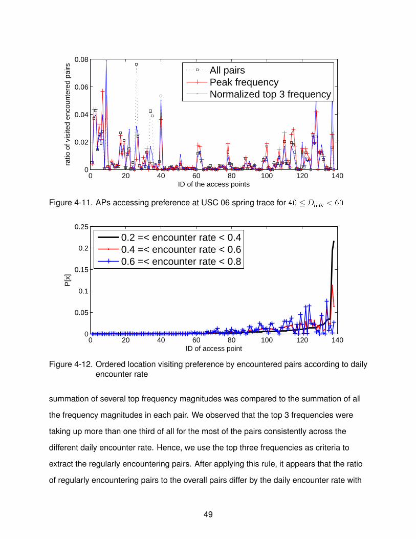
0 20 40 60 80 100 120 1400

0.02

0.04

0.06

0.08

ID of the access points

ratio

of v

isite

d en

coun

tere

d pa

irs

All pairsPeak frequencyNormalized top 3 frequency

Figure 4-11. APs accessing preference at USC 06 spring trace for 40 ≤ Drate < 60

0 20 40 60 80 100 120 1400

0.05

0.1

0.15

0.2

0.25

ID of access point

P[x

]

0.2 =< encounter rate < 0.40.4 =< encounter rate < 0.60.6 =< encounter rate < 0.8

Figure 4-12. Ordered location visiting preference by encountered pairs according to dailyencounter rate

summation of several top frequency magnitudes was compared to the summation of all

the frequency magnitudes in each pair. We observed that the top 3 frequencies were

taking up more than one third of all for the most of the pairs consistently across the

different daily encounter rate. Hence, we use the top three frequencies as criteria to

extract the regularly encountering pairs. After applying this rule, it appears that the ratio

of regularly encountering pairs to the overall pairs differ by the daily encounter rate with

49

the range being from 0.15 to 0.4. Rare encounter can hardly yield regularity due to its

small number of samples. For the opposite reason, frequent encounter often leads to the

uniform distribution of encounter, thus, any patterns are hardly noticeable especially in

daily encounter.

We first discuss the general trend of location visiting pattern at the time of encounter

events. Then, we compare the result to the regularly encountering pairs. In Figure 4-12,

the data is sorted according to the number of encounter events in the location. It is clear

from the figure that encounter events are skewed to a few locations, thus, the graph

showing exponential curve toward highly visited locations. Another observation is that

frequently encountering pairs are exhibiting different location visiting patterns from less

frequent pairs at the time of encounter events. This implies that the locations with rare

encounter events are disadvantaged in message delivery. Now we turn our attention

to the trend for the regularly encountering pairs. In the Figure 4-11, the regularly

encountering pairs are showing different visiting preference. This different location

visiting pattern supports the strong value of using regular encounter pattern. Delivery

attempt to the nodes that mainly appear in the location of scarce encounter events may

suffer from finding the forwarding nodes that have history of encounter event. Therefore,

overload on the network can be expected due to too many number of message copies.

In such a situation, 1) using the regularly encountering nodes if the encounter rate is

similar, would make more accurate estimation for the number of relay nodes to reach the

delivery probability goal and/or 2) the source node has a more chance to discover the

nodes that regularly encounter with the target node in some locations. More applications

can be developed that use such characteristics; thus, our analysis opens up for more

applications and is one of our contributions.

4.4 Temporal Stability of Mobile Encounter

In this section, we investigate the encounter history of mobile nodes and its

changes over the period of time from WLAN traces. More specifically, we conduct a

50

preliminary, yet systematic evaluation of history-based anticipation, by varying the

size of the two windows of encounter history - one former and one latter. Practically,

we compare encounter patterns in the first part of trace to the later part of trace; and

observe how well encounter anticipation works as the size of the encounter history

changes. Our findings indicate that encounter patterns of rarely meeting nodes are

surprisingly quite consistent in general, whereas frequently encountering nodes tend

to be inconsistent. Further, more encounter history appears to help to obtain better

consistency in encounter anticipation. Based on daily encounter patterns, the encounter

rate difference is generally less than 20% between two windows. Encounter rate

difference is even smaller (less than 10%) for regularly encountering pairs.

4.4.1 Stability Window of Encounter History

Knowledge about the past encounter pattern between two mobile nodes can

be beneficial in Encounter prediction can be beneficial in message bundle delivery

especially in a situation where mobility is not random. Proper use of encounter history

can be helpful in prediction of encounter in case the future encounter may base on the

past encounter. For this reason, there are multiple literatures proposing routing protocols

using encounter history (or contact history as similar terminology) [4, 5, 13, 14]. In-depth

analysis on encounter pattern can help the routing protocols to operate more efficiently

by sophisticatedly selecting the relay nodes. To help in routing, we investigate the

encounter stability, which shows the temporal change of encounter pattern. We believe

understanding of encounter stability and its relationship to encounter prediction is a

key in developing an appropriate contact pattern modeling of mobile nodes and routing

scheme that uses the mobile nodes as forwarding nodes. To analyze the encounter

stability in large scale, we investigate wireless LAN usage of 10,000 sample mobile

nodes from the University of Florida (1 Jan 2008 - 3 Mar 2008) and University of

Southern California (9 Jan 2006 - 11 Mar 2006). These sample nodes were chosen

randomly among around 20,000 nodes at USC and 50,000 nodes at UF.

51

��

��

��

�

Figure 4-13. Window of encounter history

To observe the difference between the first part of the encounter history and

the latter part of the encounter history, we divide the encounter history of each pair

to W1 and W2 from the original encounter history window as in Figure 4-13, where

both parameters indicate the size of the window in each of first and second period

respectively. We compare the difference of daily encounter rate for encounter pair (i , j)

between two periods W1 and W2, by providing Di� (i , j) = |Drate1(i , j)−Drate2(i , j)|, where

0 ≤ Drate1(i , j) ≤ 1, 0 ≤ Drate2(i , j) ≤ 1. To see the various trends by the encounter rate,

we first categorize the encounter pairs to five groups according to their daily encounter

rate and look into their average Di� (i , j), where 0 ≤ i ≤ n, 0 ≤ j ≤ n and i ̸= j for each

group.

4.4.2 Consistency of Encounter Pattern

Figure 4-14 shows the average difference of the daily encounter rate in each of UF

and USC trace according to the different dates of the break point, td , for the first window.

Each graph shows the change of Di� according to the length of encounter history,

W1. Specifically, the X-axis indicates the size of the first window W1 in days, while the

Y-axis is the average difference of encounter rate between the two windows W1 and

W2. The size of the second window W2 was set to 21 days to compare the encounter

rate of three weeks period. Bigger size of the second window W2 was discouraged

as it overlaps with the spring break period, which by the observation affects the result

meaningfully. Thus, we observed the results before the spring break time for both of

the UF and USC campus to observe the trend without the interference of significant

social context. The figures show that Di� becomes smaller as we have more encounter

history. This indicates that more history in the first window would yield the better

52

�

�

��

��

��

��

��

��

��

��

��

��

��

��

��

��

��

��

� � ��!��

��

��

A UF campus with the break point at 28th day

�

�

��

��

��

��

��

��

��

��

��

��

��

��

��

��

��

��

��

��

��

� � ��!��

��

��

B UF campus with the break point at 35th day

0

0.05

0.1

0.15

0.2

0.25

0.3

0.35

0.4

0.45

14 21 28 35 42

Av

g.

dif

fere

nce

of

en

cou

nte

r ra

te

Size of the encounter history, W1 , where td = 42

UF

0-0.2

0.2-0.4

0.4-0.6

0.6-0.8

0.8-1

Groups by

encounter

rate

C UF campus with the break point at 42nd day

0

0.05

0.1

0.15

0.2

0.25

0.3

0.35

14 21 28

Av

g.

dif

fere

nce

of

en

cou

nte

r ra

te

Size of the encounter history, W1 , where td = 28

USC

0-0.2

0.2-0.4

0.4-0.6

0.6-0.8

0.8-1

Groups by

encounter

rate

D USC campus with the break point at 28th day

0

0.05

0.1

0.15

0.2

0.25

0.3

0.35

0.4

0.45

0.5

14 21 28 35

Av

g.

dif

fere

nce

of

en

cou

nte

r ra

te

Size of the encounter history W1 (td = 35)

USC

0-0.2

0.2-0.4

0.4-0.6

0.6-0.8

0.8-1

Groups by

encounter

rate

E USC campus with the break point at 35th day

0

0.05

0.1

0.15

0.2

0.25

0.3

0.35

0.4

0.45

14 21 28 35 42

Av

g.

dif

fere

nce

of

en

cou

nte

r ra

te

Size of the encounter history W1 (td = 42)

USC

0-0.2

0.2-0.4

0.4-0.6

0.6-0.8

0.8-1

Groups by

encounter

rate

F USC campus with the break point at 42nd day

Figure 4-14. Average difference of the daily encounter rate at UF and USC campusaccording to the change of break point for the first window

53

consistency in encounter pattern. We can infer from this result that more knowledge

on the encounter history in general leads to higher consistency in anticipating the

encounter rate in the second window. Another interesting trend is Di� is greater for the

groups with more daily encounter rate. In Figure 4-14, different lines refer to different

daily encounter rates. For both UF and USC trace, it shows that the encounter rate

of the frequently encountering pairs are likely inconsistent in terms of daily encounter

rate. Note also that Di� was smallest in general when td = 28 for the same size of

encounter history W1 at both of the UF and USC traces. This implies that consistency of

the encounter rate can change depending on the break point of the two windows.

Now we move on to controlling the size of the second window. Figure 4-15 shows

the average difference of the daily encounter rate according to the change in the size

of the second window. In all of the figures, the size of the first window corresponds to

the td . For instance, W1 = 14 when td = 14 as we observe the encounter history from

the first day of the trace. Each graph shows the consistency of encounter rate between

two windows according to the change of the size in the second window for given size of

the first window. We can see from the figures that encounter consistency drops slightly,

particularly for the groups of pairs with higher encounter rate. This trend is stronger with

more history in the first window where td = 21 than less history where td = 14. In case

of UF trace with td = 14, it appears that consistency of encounter pattern becomes

better as the size of the second window grows. It is an interesting trend as in general

the consistency is expected to drop due to short length of previous history to compare.

We think the starting date of the trace may play a role in this unique trend as the starting

date of the UF trace (Jan 1) does not match to the starting date of the class date. It is

uncertain at this point, what plays a role in generating such a different trend from other

traces. We learn from this study about the varying size of the second window that with

short encounter history in the first window, the consistency in encounter pattern can be

54

0

0.05

0.1

0.15

0.2

0.25

0.3

14 21 28 35

Av

era

ge

dif

fere

nce

of

en

cou

nte

r ra

te

Size of the encounter history, W2 (td =14)

UF

0-0.2

0.2-0.4

0.4-0.6

0.6-0.8

0.8-1

Groups by

encounter

rate

A UF campus with the break point at 28th day

0

0.05

0.1

0.15

0.2

0.25

0.3

14 21 28 35

Av

era

ge

dif

fere

nce

of

en

cou

nte

r ra

te

Size of the encounter history, W2 ( td= 21 )

UF

0-0.2

0.2-0.4

0.4-0.6

0.6-0.8

0.8-1

Groups by

encounter

rate

B UF campus with the break point at 35th day

0

0.05

0.1

0.15

0.2

0.25

0.3

14 21 28 35

Av

era

ge

dif

fere

nce

of

en

cou

nte

r ra

te

Size of the encounter history, W2 (td = 14)

USC

0-20

20-40

40-60

60-80

80-100

Groups by

encounter

rate

C USC campus with the break point at 35th day

0

0.05

0.1

0.15

0.2

0.25

0.3

0.35

0.4

14 21 28 35

Av

era

ge

dif

fere

nce

of

en

cou

nte

r ra

te

Size of the encounter history, W2 ( td = 21 )

USC

0-20

20-40

40-60

60-80

80-100

Groups by

encounter

rate

D USC campus with the break point at 42nd day

Figure 4-15. Average difference of the daily encounter rate at UF and USC campusaccording to the change of break point for the second window

unpredictable. With larger encounter history and proper break point (td = 21), encounter

consistency decreases as the size of the second window grows.

4.4.3 Application of Encounter Stability Analysis

Knowledge on consistency of encounter behavior can be beneficial for developing

an intelligent message bundle delivery system, particularly where encounter patterns

amongst mobile nodes are not random. Proper use of encounter history can be helpful

in measuring consistency of encounter pattern. For this reason, there are multiple

55

0

0.05

0.1

0.15

0.2

0.25

0.3

0.35

52 59 66 73 80

Av

era

ge

dif

fere

nt

of

en

cou

nte

r ra

te

Size of encounter history, W1

regular

irregular

Figure 4-16. Average difference of the daily encounter rate at USC campus according tothe change of size for the first window of encounter history

literatures proposing routing protocols using encounter history; however, in-depth

analysis on the encounter patterns according to the differences in encounter history has

been in need to devise a sophisticated protocol that reflects the real encounter pattern.

Our analysis provides a basis for developing protocols that utilize encounter history

for determining relay nodes as well as efficient buffering and caching in the forwarding

mobile nodes.

4.4.4 Comparing Regular Encounter to Non-regular Encounter

We shall investigate the encountered pairs regarding their consistency of encounter

pattern. We use the approaches we propose in above section to find the regularly

encountering pairs from the first part of the encounter history. We also use a new

approach that divides the first window of encounter history to several pieces to see the

consistency in them. In this new approach, encounter consistency is compared within

the first window and we select the regularly encountering pairs from the pairs showing

more consistency in the first window.

56

We compare the regularly encountered pairs with the non-regularly encountering

pairs. By definition, regularly encountering pairs are much more likely to maintain

consistent encounter each other than irregular pairs on a regular basis. We used

the new approach of selecting the regularly encountering pairs by the evaluation of

consistency for the two divided windows in the first window. Encountered pairs with less

than 0.5 of difference in these divided windows were chosen for regularly encountering

pairs. The rest of the encounter pairs were considered irregularly encountering pairs.

In Figure 4-16, we observe the overall consistency between two windows and compare

between regularly encountering pairs and non-regularly encountering pairs. We look at

the pairs with at least one encounter event for both of the regular and non-regular cases.

It shows that the regularly encountering pairs have significantly better consistency

over the irregularly encountering pairs. Regularly encountering pairs show the

average difference of encounter rate between the two windows is around 0.1, which

is surprisingly consistent. Whereas, the non-regularly encountering pairs show relatively

large inconsistency with an average of 0.3 at the different of encounter rate between two

windows. This implies that the regularly encountering pairs in the first period of the trace

tend to maintain similar encounter rate in the second period. Note that the pairs with

very low encounter rate can skew this overall trend. Further analysis in the future to this

result is observing the encounter consistency by the groups of different encounter rate.

4.5 Long-term Bluetooth Trace Analysis

In this section, we analyze the long-term Bluetooth contact trace of a mobile user.

An anonymous mobile user carried our Bluetooth contact-measuring device over

6 months period and we analyze the individual encounter data. Note that this data

includes the Bluetooth contacts occurred during the mobile user’s travel. Therefore,

while this data does not reflect the accurate description of user’s contact behavior in one

location, it captures overall contact pattern regardless of location.

57

0 50 100 150 2000

0.01

0.02

0.03

0.04

0.05

0.06

0.07

0.08

0.09Time Series for Mean Value of Daily Encounter in a Bluetooth Trace

Day

Dai

ly E

ncou

nter

(bi

nary

pro

cess

)

A Encounter days

0 50 100 150 2000

0.1

0.2

0.3

0.4

0.5

0.6

0.7

Day

Time Series for Mean Value of Number of Encounters in a Bluetooth Trace

Num

ber

of E

ncou

nter

s

B Encounter frequency (count)

0 50 100 150 2000

20

40

60

80

100

120

140

160

180

200Time Series for Encounter Duration in a Bluetooth Trace

Day

Enc

ount

er D

urat

ion

(min

utes

)

C Encounter duration

Figure 4-17. Time series data for the mobile user’s Bluetooth encounter

Figure 4-17 shows the time series data for the mobile user’s Bluetooth encounter.

All the metrics (encounter days, frequency and duration) show similar trend in peaks.

Figure 4-18 shows the CDF for the size of encounter days, frequency and duration.

It shows around half of encounter events belong to very low magnitude. About 5% of the

encountered nodes throughout all the metrics show high degree of encounters.

In the figure 4-19, spectral analysis shows that periodical pattern is not as strong

as shown in WLAN trace analysis and short-term Bluetooth analysis. Particularly,

encounter duration shows very weak periodical pattern. Possible reasons could be a

break period such as vacation, summer break and international travel. We learn from

58

100

101

102

103

0

0.1

0.2

0.3

0.4

0.5

0.6

0.7

0.8

0.9

1

x: number of encountered days

P(X

<x)

Empirical CDF for Encounter Days in the BT Trace

A Encounter days

10−3

10−2

10−1

100

101

102

0

0.1

0.2

0.3

0.4

0.5

0.6

0.7

0.8

0.9

1

x: average number of encounters per day in log scale

P(X

< x

)

Empirical CDF of Average Number of Encounters per day in a BT Trace


10−2

10−1

100

101

102

103

0

0.1

0.2

0.3

0.4

0.5

0.6

0.7

0.8

0.9

1

x: encounter duration in minutes in log scale

P(X

< x

)

Empirical CDF of Encounter Duration per Day in a BT trace


Figure 4-18. Empirical CDF for each encounter metric with encountered nodes in thelong term Bluetooth trace

this analysis that periodicity may change over time and may yield different result than

short-term analysis.

4.6 Conclusions and Future Work

We investigate a WLAN trace and Bluetooth trace to discover periodicity of mobile

encounter pattern. Our analysis shows that spectral analysis can apply to analyze the

periodicity and the result shows that weekly encounter pattern is strong over most of

the traces. We also show the stability of encounter pattern over a semester period and

show the difference of encounter pattern over time. Encounter rate difference between

the first period and second period increases as the size of the window increases. In

our long-term Bluetooth contact analysis, we analyzed over 180 days of trace for a

single mobile user. It appears that periodicity is weaker than WLAN trace and short-term

Bluetooth trace. This shows that an observation for a short period can differ from a

59

0 20 40 60 80 1000.95

1

1.05

1.1

1.15

1.2

1.25

1.3

1.35

1.4

Frequency (2−93)

Mag

nitu

de

Periodicity for Daily Encounter in a Bluetooth trace

A Encounter days

0 20 40 60 80 1003.5

4

4.5

5

5.5

6

6.5

Frequency (2−93)

Mag

nitu

de

Periodicity for Number of Encounter in a Bluetooth trace


0 20 40 60 80 1001500

2000

2500

3000

3500

4000

4500Periodicity for Encounter Duration in a Bluetooth trace

Frequency (2−93)

Mag

nitu

de


Figure 4-19. Spectral analysis of long-term Bluetooth encounter for each metric

long-term period. Future work includes the application of using these periodic properties

in mobility prediction [41] [42] [43]. Overlay networks amongst the periodically contacting

pairs is one direction to study as an application. Another application is anticipating the

user’s contact with certain nodes based on regularity and stability of encounter pattern

for the pair.

60

CHAPTER 5CAPTURING AND EMBEDDING PROFILES OF MOBILE NODES

In the previous chapter, we have analyzed the encounter patterns of mobile nodes.

Result of such analysis informs of group behavior analysis of encounter patterns. We

discuss the idea of capturing periodic properties from mobile users’ contact pattern. We

then discuss the encounter community profiles of mobile nodes and their community

pattern. Our goal of encounter profile creation for mobile nodes is to emulate human

behavior in terms of community based encounter pattern.

5.1 Introduction

Mobility profile of the mobile nodes can be an useful in message delivery for

deciding targets of the message when there are multiple recipients in profile based

protocols such as profile-cast [3], bubble-rap [5] and social aware networking [4]. Those

protocols use the profiles of similarity in location visiting preference and community

property constructed based on the similarities in location visiting preference. Our work

focuses on capturing periodic human encounter pattern and their community distribution.

Location-based profiling has been studied but encounter based profiling has rarely been

studied, particularly focusing on periodic properties. Encounter pattern is important

information for encounter pattern modeling and message propagation system, where

location information is non-existent. For instance, Bluetooth encounter history does not

have location information without the help of GPS or WLAN access record with APs.

Both of GPS and WLAN quickly consume the battery of mobile devices; thus, having

the Bluetooth or short-range communication device for this specific communication

will have an advantage in battery consumption. Besides, there are frequent occasions

or many places where location information is unavailable (i.e. inside a building where

GPS does not work and APs are not installed). Moreover, message delivery or actual

encounter between mobile nodes should occur when they are in proximity of wireless

communication. Encounter event may not occur even if two nodes are accessing the

61

same location unless they are in close proximity. Therefore, study on the encounter

pattern excluding location information has several advantages over location-based

analysis.

5.2 Related Work

Profiling of mobile users was studied in many literatures based on user mobility

[44] [45]; however, little effort has been made for profiling based periodicity of contacts.

We use spectral analysis [46] to reveal the periodicity and group mobile users based

on periodical contact pattern. With an understanding of human contact pattern and

their periodic properties, we capture most important characteristics and show that

it can replicate the real-world contact pattern in terms of periodicity. Community

structure in mobile users has been critical subject of study [47] [48] [49]; yet little

is known. Revealing and capturing community structure are important works as

community information can be used in interest-based message forwarding [3] [50]

[51] or finding critical nodes for data propagation [5] [52]. Researchers showed that

mobile users’ mobility could be grouped into communities. The distribution of group

sizes by hierarchical clustering appeared following a power-law distribution in [1]. We

define encounter vector and analyze encounter trace to find communities in encounter

pattern. We also apply the hierarchical clustering to the mobile users’ contact pattern

and discover the existence of power-law distribution.

5.3 Modeling Encounter Periodicity with Profile

With the properties of encounter pattern discussed above, we propose the

encounter model for mobile nodes. TVC model provides the input of periodicity among

mobile nodes. However, TVC model does not generate the periodicity of encounter

pattern that emulates the observed encounter pattern. Instead, it takes the community

structures found from the mobility traces. With a basis on the understanding of individual

encounter periodicities, synthetic trace that emulates the real-world human encounter

pattern can be constructed (i.e. reflecting the notable weekly encounter pattern). There

62

0 200 400 600 800 1000 1200 1400 1600 18000

0.1

0.2

0.3

0.4

0.5

0.6

0.7

0.8

0.9

1

Nodes

F(x

)

Empirical CDF of maximum frequency

Figure 5-1. CDF of top 7 maximum frequencies from the 2000 sample pairs with dailyencounter rate between 0.2 and 0.4 for 128 days of UF 07 trace

are two types of implementation of periodicity generator: 1) Periodicity of individual

encounter pattern that reflects overall statistics of individual encounter 2) Periodicity

of encountered pairs. There is a trade-off in each type of trace generator. The first

type generates a trace data with overall individual encounter pattern. This reflects the

periodicity of encounter; yet, it is limited to individual encounter pattern. The second

type generates the periodicity for each encountered pair, which emulates the closely

real-world encounter events. However, implementing periodicity for each encounter pair

incurs cumbersome implementation.

Figure 5-1 shows the CDF of top 7 maximum frequency from the 2000 sample

encounter pairs for 128 days. In the figure, the knee also appears for 9% of all

frequencies which indicates roughly 7 frequencies out of 63 are dominating trend.

This implies that top 7 frequencies can be used as a signature frequency for periodicity

vector. This saves the size of vector from 63 to 7. As top 5 locations were chosen in

mining based on location visiting preference work [1], periodicity vector can be built

63

accordingly to represent the periodicity of pairs. We leave the actual construction of

vectors to future work.

5.4 Discussion of Routing Based on Encounter Profiles

In this section, we discuss the future application of periodic properties. Actual

implementation using periodic properties is out of scope. We describe the details of how

implementation can be done only. Encounter consistency may differ by the encountered

pairs. Our results show that the encountered pairs with consistent encounter rate in

the first window are likely to keep the similar encounter rate in the subsequent window.

Assuming the encounter history in the first window is the past events and the break

point is the current time where routing decision is made, the second window of the

encounter history is translated into the future encounter. In this scenario, consistent

encounter pattern in encounter history infers that the future encounter pattern is also

likely consistent to the encounter history. With this idea, routing decision of selecting

forwarding node can be made by looking at the encounter history and its consistency

for finding consistent encounter pattern. In addition to the consistency of encounter

pattern, encounter probability is calculated based on the encounter history. Prophet

uses the encounter count for next encounter probability based on encounter history

for finding relay nodes of a message bundle. However, how to calculate the probability

of encounter is unclear. For instance, encounter count can have burst pattern that

yields biased results in probability. We overcome this problem by using binary time unit.

We divide the time series data according to the defined time units depending on the

scenarios. For instance, hourly encounter is a time series data with time unit of an hour

with a value of 1 in the presence of encounter event within an hour. Different time units

can be appropriate depending on the scenarios. Selecting the regularly encountering

nodes is a critical decision in this routing scheme. The irregularly encountering pairs

may not be appropriate for probability calculation because their encounter history is

inconsistent; thus, their future encounter is unpredictable. Furthermore, the randomly

64

A

DB

C

E

F

ε (BD)

ε (BE)

ε (EF)

ε (BC)

ε (AB)

ε (AC)

ε (CD)

ε (CF)

Regular encounter

Non-Regular encounter

ε: regularity metric

Figure 5-2. Overlay networks using periodicity as a link weight

encountering pairs are also not good candidates for message forwarding as their

behavior can not be estimated. Therefore, interest of calculating probability based on the

encounter history lies in the regularly encountering nodes. How much of non-regularly

encountering pairs should be factored in decision differs by scenarios.

Figure 5-2 shows an example scenario of a network with links weight decided by the

strength of regularity. Application of this network can be periodical news, information or

electronic coupon to the subscribers via the regularity based overlay networks. Using

MobiTrade [22], the data can be shared with incentives for sharing more data via this

overlay networks. This overlay networks can also be used in establishing the level of

encounter based trust such as PROTECT [29] [30] [31] by augmenting the encounter

based trust metric with the addition of periodicity metric.

5.5 Community Profiles of Mobile Users

In this section, we discuss the clustered behavior of mobile nodes from real-world

traces. Profiling mobile users based on location-visiting preference was introduced in

[1]. Our analysis is performed for contact behavior of mobile users. We first describe

the previous finding from the location based profile work, and explain the approach to

65

Figure 5-3. Example of embedding profiles in various interfaces

discover contact based profile. Then, we compare the results to reveal the power-law

distribution in group (community) sizes from both types of profiles. These profiles

can be embedded on autonomous nodes. Examples are shown in Fig. 5-3. In our

implementation for autonomous mobile nodes, power-law distribution that we discover

from both types of profiles is used to assign community IDs. Note that only the analyzed

result (i.e. power-law distribution) is used in this work instead of embedding either

type of profiles directly though they can be embedded in our testbed. Complicated

community structures such as overlapping community model is studied in [53] [54],

however, community modeling is not out of scope in this dissertation.

5.5.1 Location Visiting Preference

[1] shows that mobile users can be clustered by their location-visiting pattern.

Behavioral signature of location-visiting preference for a mobile user can be built by an

association matrix as in Fig. 5-4 (courtesy of Hsu [1]). For each day i , each row saves

the duration of time at each location j . Percentage of time spent in each location j is

put in each column of the matrix. Each matrix is condensed to a vector representation

66

OfficeDorm

úúúúúú

û

ù

êêêêêê

ë

é

ntt

ji

xx

x

x

,1,

,

1,2

1.04.05.0

LLL

MOM

MM

MO

LL

Each row represents the

percentage of time spent at

each location for a day

Each column corresponds to a location

An entry represents the percentage of

online time during time day i at location j

Figure 5-4. Location based association matrix for each mobile user (courtesy by Hsu [1])

of most significant behaviors by performing Singular Vector Decomposition (SVD).

Similarity score is produced for the encountered nodes. Each node can make a decision

based on this similarity score whether the encountered nodes show similar behavior to

a target group. Profile-cast [3] uses this location signature for delivering messages to

target group of nodes. If implemented on robots, they can build the same association

matrix by collecting its own location-visiting information. Profile-cast was implemented

on Nokia PDA; therefore, it is directly usable in our testbed without further modification.

5.5.2 Encounter Vector

To analyze encounter pattern of mobile users, we define an encounter vector. An

encounter vector, Vi , for user i , represents an encounter behavior of the mobile user i

with all other nodes. Specifically, each element in a encounter vector indicates a ratio of

encounter in days with a mobile user. Note that different metrics such as encounter rate

or duration can be used but we use encounter days [46] in this work. For mobile user, i ,

total days of encounter, Ti is calculated as in the following (5–1), where M is a number

of total nodes, N is a number of total observed days in trace and Ed(i , j) indicates a

binary process of encounter between a node i and j in a day d .

67

Ti =

M∑j=0

N−1∑d=0

Ed(i , j) (5–1)

Using the sum of total encounter, Encounter vector, Vi , is formed in the following

way to reflect the ratio of encounter with each node:

Vi = {N−1∑d=0

Ed(i , 0)/Ti , ......,

N−1∑d=0

Ed(i ,M)/Ti} (5–2)

Now we analyze the real-world trace using this vector representation of encounter.

USC 06 and UF 07 traces [35] are used for analysis.

In [1], the mobile users show power-law distribution in size of groups with hierarchical

clustering according to their location visiting vector as shown at log-log scale representation

in Fig. 5-5. We also apply the same hierarchical clustering to mobile users’ contact

pattern based on proposed encounter vector. The result shows the size of ranked

groups for contact pattern also follows power-law distribution as shown in Fig. 5-5.

Specfically, slope of -1.48 reflects the distribution of contact based group sizes. In the

following section, we explain how to implement self-decision making mobile nodes while

following this community distribution pattern. With this understanding of community

distribution, we introduce the process of embedding community information according to

power-law distribution.

5.6 Conclusions and Future Work

We discuss the profiling process of mobile users based on periodicity of contact.

We describe the process of generating a contact periodicity that matches to real-world

statistics. In addition, we define encounter vector and show that real-world contact

pattern in groups follows power-law distribution in terms of rank group size, which

is the pattern observed from grouping by location visiting preference. Future work

includes exploring more properties of community exist in social contact pattern such

as communities based on contact duration or frequency. Selected groups (i.e. highly

68

1 10 100 10001

10

100

1000

10000

User group size rank

Gro

up s

ize

UF

1406*x−1.48USC

500*x−1.48

A Clustering by encounter pattern

U ser g roup size rank

Gro

up s

ize

1

1 0

1 0 0

1 0 0 0

1 1 0 1 0 0 1 0 0 0

D a rtm ou th5 4 0 *x^-0 .6 7

U SC5 0 0 *x^-0 .7 5

B Clustering by location-visiting pattern (Courtesy of Hsu [1])

Figure 5-5. Ranked size of groups after grouping by hierarchical clustering for campustraces. Both graphs fit a power-law pattern for the size of groups.

69

active users) can be grouped separately. Studying community groups based on location

visiting preference and encounter pattern to see the similarity and difference will provide

valuable knowledge in understanding community structure of mobile users’ society.

70

CHAPTER 6DESIGN OF A MOBILE SOCIAL NETWORKING TESTBED

6.1 Introduction

Recent advances in mobile networks brought marriage of social and mobile

networking, which is going to constitute the future frontier with the proliferation of

smartphones. Growth of mobile social environments requires appropriate networking

protocols and services using human social pattern. To evaluate such protocols and

services, it is essential to have a large-scale and realistic testing environment, including

simulations and testbeds, which incorporate various aspects of mobile user behavior.

Toward tackling these challenges, we introduce a novel mobile networking testbed,

where autonomous mobile nodes collectively mimic human community contact pattern.

Specifically, we discover power-law distribution in group sizes from contact pattern and

use it for contact profiles. Furthermore, we develop several contact rule-based decision

criteria for autonomous mobile nodes. Our simulation for 1000 mobile nodes shows that

mobile nodes can match human community contact pattern. In addition, we implement

a prototype testbed by embedding the same decision criteria on mobile robots. To

the best of our knowledge, our work is the first to embed community information from

real-world data analysis on autonomous mobile nodes, in either simulation or testbed.

Our findings provide opportunities for building realistic testbeds with autonomous mobile

nodes for various types of mobile social networks and services. With proliferation of

mobile devices and social network services, it is important to have an environment to

test new networking protocols and services using mobile users’ mobility. Realistic mobile

networking testbed is important for such a mobile networking environment as breakdown

of links due to mobility creates challenging issues both for Mobile Adhoc Networks

and wireless sensor networks [55]. Towards realistic testbed for mobile networks, we

address the following three key challenges: 1) Testing environment should support

realistic movements of mobile nodes based on real-world mobility data. Particularly,

71

we intend to capture mobile users’ community-based contact pattern. 2) Autonomous

mobile nodes make their own decisions while emulating human mobility. Existing

testbeds are limited to random mobility and predefined paths. Other simulation and

mobility models can capture realistic human mobility; yet, they require having global

knowledge, including location of other nodes. This knowledge may not be available to

every node in a real mobile networking environment. Hence, mobile nodes need to be

able to decide their own movements based on available information in real time. 3) Both

of simulation and prototype implementation on real mobile nodes should be available.

Simulation provides easy adjustments for experiment parameters and profiles of mobile

nodes along with visualization. On the other hand, prototype implementation shows the

feasibility of deployment. Note that we interchangeably user the term, contact, encounter

and meeting, all in the same context of physical closeness that is sufficient for direct

wireless communication (i.e. Bluetooth discovery) as in [46] [16] [56] [57].

Existing mobile networking testbeds use robots, emulation or mobility modeling

to deploy mobile nodes’ mobility [24] [23] [26] [27]. Robots are deployed in random

mobility or predefined paths. Emulation of robot movements follows the same criteria

and requires to have location information. Modeling needs global knowledge of node

location to generate mobility and contact statistics. To deploy on the autonomous mobile

nodes that collectively mimic mobile encounters in real world, it is essential to have a

mobility profiles and self-decision making criteria for each node. This approach enables

to embed the algorithm both on simulated mobile nodes for large-scale experiment and

on physical mobile nodes (i.e. robots).

In order to achieve this goal, we develop contact rule-based decision criteria

that are embedded on each mobile node to make a mobility decision for themselves

upon contacting other mobile nodes. Furthermore, we investigate real-world network

trace to reveal the community distribution based on contact pattern. We discover

power-law distribution for the size of groups from community contact pattern, and

72

Emulation

Community of Mobile

Users

Controlled! Chaotic!

Figure 6-1. Bridging the gap between the emulated controlled environment (network ofrobots) and the non-controlled chaotic real mobile world (participatornetworks). Both environments are connected via mobile devices that enablecommunication between these environments. Robots move with mimickedhuman mobility, thus, emulating real chaotic world without needing to recruithuman participants

assign community information to the mobile nodes accordingly. In addition, we embed a

scheduler to emulate periodical contact with community members. Finally, we evaluate

with multiple metrics including contact days, frequency and duration compared to

real-world contact pattern that is processed from campus network trace.

Another part of our work is a proposal of novel idea for a realistic mobile networking

testbed that can blend a network of robots and participatory networks. The concept of

bridging two different environment of controlled and uncontrolled was discussed in our

earlier work [58] and shown in Fig. 6-1: 1) A network of robots is a swarm of robots that

roam around with wireless communication devices for opportunistic communication. 2)

Participatory network is a network space where participants in the experiment carry the

mobile devices as human cohorts.

73

Both of these environments have limitations: In a network of robots, robot mobility

is often limited to the lab environment space. Moreover, current testbeds support

random mobility and predefined mobility paths, which are unrealistic to emulate human

mobility. Participatory network is an ideal form of testing environment if sufficient size

of target population is willing to cooperate in the experiment. However, it brings issues

of recruiting appropriate participants and control of human cohorts, particularly if the

sample size is big. To bridge the gap between these two types of the testbeds and

take the strengths of both, we propose to embed a personality profile on the robots.

Specifically, it can contain the rule-based decision criteria and community profile

information on the robot mobile nodes. We provide implementation details of this

bridging effort using iRobot Create and Nokia PDA, which is a prototype of mobile social

networking testbed.

Our main contributions in this work are 1) designing a contact rule-based decision

criteria for autonomous mobile nodes in both of simulation and robots; 2) applying a

real-world community data on the mobile nodes that emulate collective group behaviors;

3) proposing a novel architecture of realistic mobile networking testbed that bridges the

gap between controlled testbed (networks of robots with fixed mobility) and uncontrolled

testbed (participatory testing); and 4) implementing a prototype for the network of

autonomous robots.

6.2 Related Work

There are three parts of related works: 1) analysis of human behavior, 2) participatory

networks, and 3) mobile networking testbeds.

6.2.1 Analysis of Human Mobility

Related subject of human behavior research in relation to networking is social

behavior of human mobility. Several networking protocols using communities and social

behavior have been proposed including Profile-cast [3], SimBet [4], BubbleRap [5],

PRO [50], SIMPS [59] and SANE [60]. The results in these works were evaluated via

74

random mobility simulation and real-world trace. Experiments on simulation or testbed

using autonomous mobile nodes can provide extended testing environment for such

protocols. To create such an environment, it is critical to understand human mobility

and their social interaction pattern. Using real-world networking traces, many studies

focused on finding inter-contact time and location visiting pattern of mobile users to use

in modeling human mobility and its social interaction pattern [28] [9] [16] [12] [15] [61].

Research findings from these studies are foundations of creating a testbed that takes

human-like interaction between mobile nodes. Yet, it is unclear how to adapt the mobility

models on the autonomous mobile nodes, which do not have knowledge of location of

other nodes. Our profile-based approach and self-decision approach is unique in that

it can be implemented in a distributed fashion without global knowledge. This enables

implementation of the algorithm on mobile robot nodes without significant modification.

The other pattern we apply in our work is periodical pattern. Periodical pattern was

observed at aggregate location access pattern for WLAN access points and captured for

modeling in various works [47] [8]. It was studied that individual and pair-wise contact

pattern shows strong periodical trend via WLAN and Bluetooth trace analysis [46].

Following this trend, we use a scheduler that assigns on-time of mobile nodes based on

this periodical contact pattern.

6.2.2 Mobile Networking Testbeds

Our implementation part of network of robots lies within the area of mobile

networking testbed. Profile based approach can be implemented and augmented to

the existing mobile testbed by embedding the mobility profiles. iRobot is programmable

robot for research purpose that is originated from Roomba vacuum robot. It has been

used in several other testbeds and we also use this robot in the implementation of the

testbed as a mobile node. Several mobile networking testbeds use robots as mobile

nodes. MiNT [23] is a miniaturized network test-bed solely using iRobots in a controlled

space. A server computer controls the movements and communication amongst iRobots

75

that are equipped with WLAN. Although this test-bed can expand with multiple numbers

of iRobots and be effective in experiment for small-scale mobile adhoc networks, it

still suffers from scalability and diversity of nodes. Roomba MADNeT [24] showed

capability of using iRobot for DTN. They mounted a wireless router that runs on Linux

by connecting via modified serial cable. This process may take advantage of costumed

lightweight programming board to utilize wireless communication feature, specifically for

the testing purpose. However, this process can be tedious and cumbersome to many of

researchers who are not skilled in this area. Our method is simple and uses the existing

device. Connection requires the minimum step and effort: either Bluetooth pairing

or connecting a serial cable directly with a distant or attached computer. MeshTest

Wireless Testbed [25] is another DTN test-bed. They use enclosures to contain the

laptop computers and measure the signal attenuation for implemented DTN protocol.

The design is centralized and users can view the wireless nodes moving around from

the server computer. Mobility is limited to controlled environment, as the participants are

to follow the given paths and required to be in the experiment range. In our presentation,

nodes can have complete control of their movements including message propagation

decisions. Moreover, measurements are decentralized in our experiment, as each

measurement record is kept inside the mobile nodes. SCORPION [27] incorporates

various mobile devices. They use 20 iRobots along with a toy airplane and several

vehicles to test various types of mobility. They carry the specifically designed DTN

devices test the communication protocols via WLAN and Bluetooth. Random mobility

is applied for robots and toys. Other carriers move in a designed direction. Thus, it can

test the performance of DTN protocols with controlled mobility. Our design philosophy

can also be incorporated to this testbeds. SCORPION differs from our testbeds in

that we use common devices that are carried by normal human for communication

and controlling robots. The other unique feature of our testbeds is that we use profiles

to emulate real human mobility with freedoms of profile modification. In addition, our

76

participatory testing environment allows anonymous human subjects to participate in the

testing. Our community contact rule-based decision criteria for mobile nodes to make

mobility decision was influenced by Plausible mobility [62], which infers mobility trace

from encounter trace. Pursuit-evasion game in robotics [63] has two groups of mobile

nodes - pursuers and evaders. Our rule-based decision criteria also have two group of

mobile nodes - friends and strangers.

6.2.3 Participatory Networks

We define participatory Networks as a network where voluntary human participants

who use mobile devices communicate via mobile devices. Original concept is inspired

by the participatory sensing project [64]. Participatory sensing has been widely

deployed, including CenceMe [65], Micro-Blog [66] and PEIR [67]. We use a similar

idea in our Bluetooth discovery program as it collects the information for encountered

devices as a sensor. Similar experiments were performed in [38] [68]. If conducting

an experiment with participants, it is an ideal participatory testing environment for the

protocols and services that use human mobility for message propagation. Participatory

testing was partially investigated via our own Bluetooth trace collection program as well

as CrowdLab [69]. In CrowdLab, virtual machines run guest processes developed by

researchers on the volunteer’s phone. This enables an idea of participatory testing to

some extent. Other attempt along the same line is PhoneLab [70] where authors attempt

to build an environment with a thousand phones to provide usable space for testing

kernel level communication protocols.

The main strengths of profile based mobile testbed as compared to other mobile

testbeds are autonomy of participating subjects and replication of personality. Critical

feature of our testbed is that human mobile nodes can be emulated by embedding

human mobility profiles onto a network of robots; hence, we provide a controllable

environment in our testbed. This is particularly useful when researchers want to

experiment for certain target human profiles. Further, profiles and mobility decision

77

criteria is interchangeable between simulation and implementation. Hence, large-scale

experiment that is difficult to perform with mobile devices can be simulated. Additional

advantage of our testbed is that it can operate on top of the other testbeds; thus,

researchers can take advantage of existing testbeds while enhancing its performance

with the functionality of our testbeds.

6.3 Testbed Architecture

We aim to build a mobile networking testbed that can integrate controllable

experimental environment with uncontrollable crowd sourcing environment. In this

section, we discuss the design of prototype testbed using robots. We first describe

autonomous mobile nodes that are used for both in simulation and prototype implementation.

Then, we discuss the implementation details.

6.3.1 Autonomous Mobile Nodes

Autonomous mobile nodes are mobile nodes that make mobility decisions

independently upon contact events. The mobile nodes do not have global knowledge

of other nodes. They scan nearby area via wireless signal. Upon discovering other

nearby nodes, the mobile node either makes another mobility decision or establishes

communication with encountered nodes. To collectively mimic human contact patterns,

it is critical to understand group contact behavior of human. We extract contact patterns

from real-world network trace and analyze the group (community) behaviors by

clustering mobile nodes based on contact pattern. Community distribution pattern

is applied to mobile nodes as their profiles, namely, community identity information.

Mobile nodes, upon encountering other nodes, look up the community information and

make a decision based on pre-configured rules. This resembles human mobility and

its decision making of mobility. We describe this investigation of real-world community

contact pattern and rule-based decision criteria in the later section in detail. Note that

this rule-based decision criteria and community information are embedded for both of

the robots and mobile nodes in simulation.

78

Figure 6-2. Picture of iRobot, its controlling Nokia N810 PDA and human carrying NokiaN810 PDA

6.3.2 Network of Autonomous Robots

In the network of autonomous robots, robots freely move around while emulating

the movement of humans. Its mobility is decided by embedded rule-based decision

criteria and community information (ID) of contacted nodes. This rules and community

ID are programmed into the mobile devices, which we call as a personality interface

that makes the decision and controls the mobility of robots. We choose iRobot Create

for implementation. The controlling mobile device in this implementation is Nokia

N810 PDA but any other devices with Bluetooth can be used (i.e. Android, Windows

Mobile). The personality interface in the mobile device can send commands to iRobot

via Bluetooth. We mount the controlling devices on top of the robots by simply putting

on the iRobot. In this setting, we take advantage of massively produced and popular

mobile devices that are cost effective for their capabilities compared to specifically

designed hardware for research purposes. Moreover, because both of the robots and

79

humans carry the same type of mobile devices (i.e. Nokia PDA), it is feasible to use

the same communication protocols between them. Our prototype implementation is

shown in Fig. 6-2. Demonstration video is available online at [35] to show the mobility

according to contact rule-based decision. Note that although we implement a prototype

of a network of autonomous robots, our focus is on a novel idea of realistic mobile

networking testbed. This includes understanding and grouping of human contact pattern

and a heuristic rule-based decision algorithm that collectively emulates community

behavior without location information of other nodes. We discuss more implementation

details on robots in Section 7.

The only difference of mobile device at between robots and humans is that

robot-controlling device runs an personality interface process in background. Bluetooth

discovery program runs on mobile devices to search for other nearby Bluetooth devices

and find out their community IDs. The communication structure between mobile devices

on robots and human is illustrated in the Fig. 6-3.

6.3.3 Participatory Testing

The other part of the design is participatory testing. Network of Robots is limited

in scalability at both the number of nodes and size of the space because of costs and

difficulty of deployment in the large space. Therefore, robots may show limited and

unrealistic mobility. By using crowd sourcing, we can enhance the testing environment

significantly at both of the criteria. Participatory testing is a novel idea that uses human

society as testbed. Human cohorts who are voluntary participants in experiment of

networking protocols are crowd source in this testbed. Participants can download and

install the networking protocols to their devices and carry them around. With proliferation

of smartphones these days (e.g., iPhone, Android), it is easier to seek for human

cohorts.

We conduct an experiment with small set of human subjects and seek to explore the

potential of participatory testing in mobile networks. Specifically, we recruited graduate

80

Human

Communication

protocol

Personality

Profile

iRobot

Mobile Device

Communication

protocol

Personality

Profile

iRobot

Mobile Device

Communication

protocol

Mobile Device

Human

ID

(MAC)

ID

(MAC)

Mobile Device

Discovery

Mobile Device

Discovery

Mobile Device

Discovery

ID (MAC)

Command Interface Command Interface

Figure 6-3. Communication structure among robots, personality interface, andcommunication protocol

students taking a computer networking course in computer science over two semesters.

Each human subject carried either HP iPAQ (fall semester) or Nokia N800/810 (spring

and fall semesters) on campus. Bluetooth discovery program ran in each of mobile

device and recorded Bluetooth encounter every 90 seconds. Even though more human

participates in fall semester, more records are collected in spring semester because of

longer length of experiment. Whereas, more unique number of devices are encountered

in fall semester. It is worth noting that a few participants (less than three in total) fail

to record properly due to misuse of devices or their schedule to go out of town. We

81

learned from our experience that even small-scale experiment requires extensive effort

to educate the participants and we may still expect a few exceptions.

Encounter measurements have been performed by multiple research projects

such as MITs Reality Mining [61] and Haggle projects [38]. Yet, the total numbers of

participants was limited to less than a hundred. Researchers used WLAN trace as

an indirect way of measuring encounters [1, 39] because of its large sample size. We

overcome this scalability issue by publicly recruiting human subjects. Specifically, we

create a public community for the testbed so users can download the programs to

participate in the test. These participants form a large testbed. To achieve this goal,

it is essential to develop a programmable interface to make the testing easier. We

implemented communication programs on the Windows Mobile-based (HP iPAQ) and

Linux-based MAEMO (Nokia N810) smart phones.

Many scenarios and protocols can be tested through this participatory testing,

including the DTN routing protocols based on social models. The Profile-cast [3] is

one of such protocols that provide communication based on the behavioral profiles of

humans via social sensing. A message is routed based on user profiles as a function of

the users mobility preferences. The Profile-cast was tested with students in computer

networking class in 2010 spring. However, the system has yet to be tested in a public

forum, which is not our focus of this demonstration.

6.3.4 Limitation of Controlled and Uncontrolled Environment

Participatory sensing is a crowd sourcing of sensor data from voluntary participants

[64] [67]. Participatory testing is similar to participatory sensing in that it leans on

human participants; however, the task is even harder as participants should be engaged

actively in testing over certain duration of time. This involves sensing mobile contacts

and running networking protocols or services. It becomes particularly difficult when

there are too many human participants to manage. For instance, participants may

not follow the experiment instruction. Further, malicious participants may damage or

82

mislead the experiment results. Therefore, participatory testing is a chaotic environment

where considerable effort to control the testing is required, yet, may still have difficulty

in gathering correct experiment data. Hence, there is much demand for a testing

environment where realistic subjects can be used in an experiment while controllability is

supported.

Testing environment with autonomous mobile nodes provide flexibility in control

while simulating human mobility. Capturing community behavior of human mobile users

and embedding the community information as their profiles can be a step forward. In

the following section, we provide details of profiling mobile users based on real-world

data analysis and use of results in creation of rule-based decision criteria for individual

mobile nodes. We show from simulation of autonomous mobile nodes that proposed

approaches can create a realistic testing environment while collectively matching

real-world contact patterns.

6.4 Contact Rule-Based Decision Criteria

It is a challenging task to replicate the contact pattern in a distributed implementation

without location information. Heuristic mobility decision is a critical factor in this problem

as available information for mobility is limited. Plausible mobility [62] infers mobility trace

from encounter trace using draw, repulsion and attraction properties. Attraction is an

intention to move towards other nodes; repulsion is a force to move away from particular

nodes; drag is a property to stay and not to be affected by other nodes. It requires global

knowledge of all nodes’ encounter information and location information. Implementation

of draw and repulsion are viable by allowing nodes to stay away from each other when

they are supposed to encounter infrequently and making them stop when they are

supposed to encounter frequently, however, attraction property cannot be implemented

as each node does not have information of other nodes. Hence, it is not appropriate to

implement on autonomous mobile nodes that work in a distributed fashion. Adopting

83

Start

Search

for

friends

StaySlow

search

Run

away

F > 1

F = 1

F=0 &

S=0

F: # of friends

S: # of strangersS !1

F !

S/2

F <

S*2

F=0 & S=0

F = 1 & F !S/2

F = 0

F < S/2

F=1 & F !2

Figure 6-4. State diagram of friend-stranger decision model

the similar idea, however, a decision mechanism based on community information of

encountered nodes can achieve the goal.

One assumption in forming a community is that group members are decided based

on their contact duration and periodicity; thus, the objective of group member is to

find their own group members and maintain periodical contact with them. To this goal,

we use the similar ideas in plausible mobility for making decisions of next movement.

Repulsion is implemented in a way of getting away from other group members upon

encounter. Draw is triggered when encountering multiple group members. Attraction

is implemented by slowing down search speed of group members and thoroughly

searching the nearby area until finding more group members. This algorithm does

neither perfectly find all of the group members nor prevent contacts with other group

members. However, as small world in wireless networks analysis [57] shows, a few more

added links can bridge most of the disconnected networks; hence, unavoidable contacts

with other group members are still realistic.

Friend-Stranger is a decision criteria used when encountering group/non-group

members. A decision is made according to a community identity (friend or stranger) of

84

Me

Me

Me Me

Fast Search

F

Slow Search

FF

Stay

S

S

Run Away

Friend node Wireless scan rangeF S Stranger node

Figure 6-5. Mobility of source node (Me) in each decision

encountered nodes. A friend is a node belonging to the same community (i.e. group

members) and all other nodes are considered as strangers (i.e. non-group members).

As discussed in the previous section, a node meets friends for more than certain time

duration, while meets strangers for a short time.

The state diagram in Figure 6-4 shows four states that are included in the decision

criteria. Me is the node that is making a decision in this case; however, note that other

encountered nodes also make their own decisions as Me node does. Four scenarios are

introduced: 1) When there are no nodes nearby, Me is in a search mode, which makes

the Me node to move with fast speed in square shape direction. 2) Upon encountering

a friend, Me goes into a slow search mode where it assumes there might be other

friend nodes around and slows down the speed of search. Further, the node moves in

octagon shape direction to search the area thoroughly. 3) When Me discovers multiple

85

friend nodes, Me stops and holds the position because this indicates that Me probably

is located inside a friend community. 4) When there is far more number of strangers

than friends, Me escapes from the current position by going into a run-away mode. It

moves backward to move out of the area full of strangers. Additionally, friend nodes

that contacted more than duration threshold are considered as having a full contact.

This means there is no need of maintaining contacts with the same node; thus, they

are considered as strangers though their community information still indicates that

they belong to the same community. This ensures the nodes to move around without

being stuck in one place to contact the same nodes repeatedly. In this presentation,

the threshold for duration is 240 minutes per day. Mobility of source node in each

decision is described in Figure 6-5. Proposed decision model, however, has limitation

as staying in a community can lead to missing out opportunities to contact with other

community members. We proposed this model in our poster presentation [71] with

uniform distribution. The model was able to mimic contact duration and periodicity,

however, did not capture the contact days and frequency. We introduce several methods

to improve in this area so that the group contact behaviors show closer contact pattern

to real-world trace in multiple metrics.

6.4.1 Power-law Distribution

Our new discovery of power-law distribution for the sizes of the communities can

lead to a different result than previous implementation of uniform distribution. Unlike

equal number of community members for each community, community IDs can be

assigned to follow the power-law distribution. Specifically, distribution of community

sizes can follow the slope of -1.48 in log-log scale that matches group sizes from contact

pattern. Another improvement to generate close results to real-world contact pattern

comes from modified rule-based algorithm. Instead of staying in one location upon

encountering multiple community members, a node can choose to explore the area to

move toward a location where more members can be found. The same logic applies

86

Table 6-1. Properties in each node’s profileProfile Property DescriptionContact frequency For contacted nodesContact duration For contacted nodeson-off Day in days of a weekon-off Time in a day

to a slow search mode, where it can support of movement to a location where more

community members are found after thorough search instead of stopping immediately

upon discovering multiple nodes. This improvement brings more contacts with

community members that the node is already contacting as well as the opportunities

to contact with other nearby members.

6.4.2 Memory

Adding a memory to remember the location where a node has contacted the most

number of nodes recently can help the node to avoid unnecessary contacts with other

strangers. Thus, having a Memory to remember allow mobile nodes to show more

contacts with friends compared to contacts with strangers.

6.5 Experiment

In his section, we report the experiment results of simulation compared with

real-world contact trace (UF trace) [35].

6.5.1 Simulation Setup

Parameters for simulation is made close to a real world mobile network trace.

6.5.1.1 Community profile

Each mobile node maintains its own contact profile. Table 6-1 shows the properties

in a profile. Each node records contact days, frequency and duration with other nodes

in its profile, which is used to determine a full contact. in addition, on-time information is

carried by each mobile node, which we explain in the following section.

6.5.1.2 On-time scheduler

Study shows that contact pairs exhibit periodical encounter from analysis of WLAN

users and Bluetooth contacts by mobile users [46]. To emulate this behavior, we adopt

87

Table 6-2. Scheduler for on-time periodDaily schedule ProbabilityDay time (9am-5pm) 0.98Evening time (5pm-1am) 0.017Dawn time (1am-9am) 0.003

Table 6-3. Scheduler for on-time durationOn-time duration Probability0-8 hours 0.78-16 hours 0.216-24 hours 0.1

a scheduler to each mobile node. As shown in Table 6-2, a node has on-off day in a

week and on-off time in a day. Each node is assigned random on-off time in a day and

week. In addition, to reflect a realistic schedule, different weights are put for starting time

of a day, on-time duration of a day and between weekdays and weekends. Parameters

for on-time with a weight in daily schedule is shown in Table 6-2. For weekdays, a

node is given 99% chance to be active for each day and 1% chance to be active during

weekends. Scheduler for on-time duration shows in Table 6-3.

Nodes appear between 0-8 hours with probability of 0.7, 8-16 hours with 0.2 and

16-24 with 0.1. These values are from human observation and not obtained from the

traces; thus, they do not accurately reflect the trend in the network traces.

6.5.1.3 Environment setup

Table 6-4 shows the environment set up for simulation and UF trace. Number of

communities is set to the total number of nodes 20 = 50. Speed of slow search is 10

meters/min and 40 meters/min for fast search and run away mode. Each mobile node

scans 40 meters of radius to discover other nodes. In UF trace, nodes that showed for

Table 6-4. Experiment environment (UF data is an approximate value.)Domain Simulation UF traceSpace 1000 meters 5000 metersNodes 1000 1000Period 64 days 64 daysCommunities 50 50Granularity 10 seconds 1 second

88

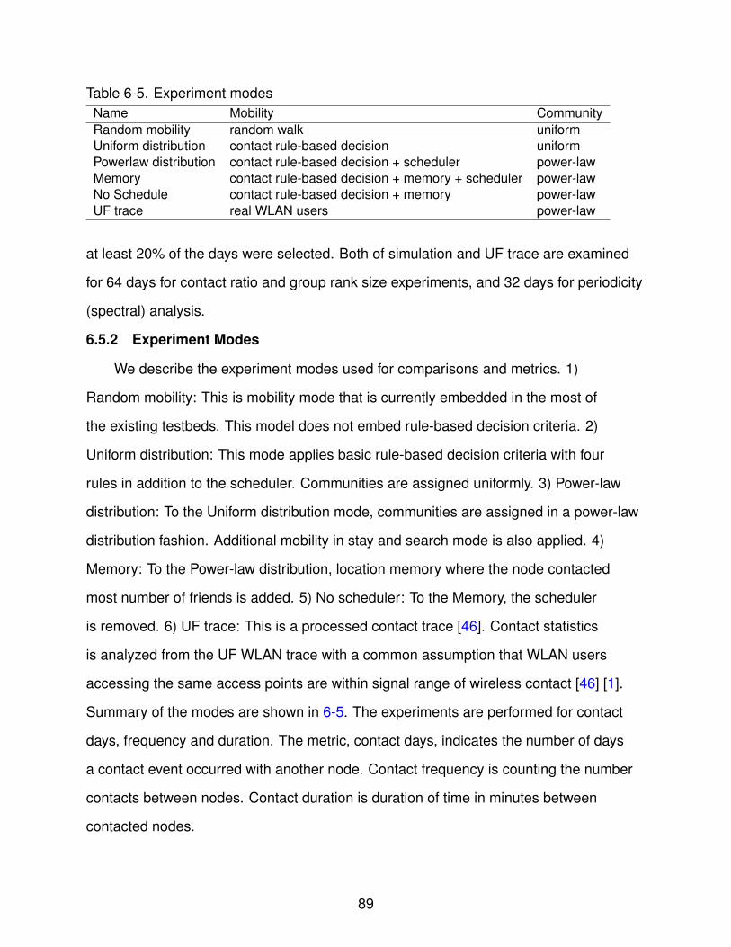
Table 6-5. Experiment modesName Mobility CommunityRandom mobility random walk uniformUniform distribution contact rule-based decision uniformPowerlaw distribution contact rule-based decision + scheduler power-lawMemory contact rule-based decision + memory + scheduler power-lawNo Schedule contact rule-based decision + memory power-lawUF trace real WLAN users power-law

at least 20% of the days were selected. Both of simulation and UF trace are examined

for 64 days for contact ratio and group rank size experiments, and 32 days for periodicity

(spectral) analysis.

6.5.2 Experiment Modes

We describe the experiment modes used for comparisons and metrics. 1)

Random mobility: This is mobility mode that is currently embedded in the most of

the existing testbeds. This model does not embed rule-based decision criteria. 2)

Uniform distribution: This mode applies basic rule-based decision criteria with four

rules in addition to the scheduler. Communities are assigned uniformly. 3) Power-law

distribution: To the Uniform distribution mode, communities are assigned in a power-law

distribution fashion. Additional mobility in stay and search mode is also applied. 4)

Memory: To the Power-law distribution, location memory where the node contacted

most number of friends is added. 5) No scheduler: To the Memory, the scheduler

is removed. 6) UF trace: This is a processed contact trace [46]. Contact statistics

is analyzed from the UF WLAN trace with a common assumption that WLAN users

accessing the same access points are within signal range of wireless contact [46] [1].

Summary of the modes are shown in 6-5. The experiments are performed for contact

days, frequency and duration. The metric, contact days, indicates the number of days

a contact event occurred with another node. Contact frequency is counting the number

contacts between nodes. Contact duration is duration of time in minutes between

contacted nodes.

89

Fast search

/Run away

Slow search

Stay

Community 1 Community 2

Figure 6-6. Simulation tool shows the mobility and encounter of autonomous mobilenodes. Each circle indicates a signal range to detect other nearby mobilenodes. Each community is identified by different colors. Extra empty innercircle is for the nodes in slow search mode. Nodes that are holding in thecurrent positions are displayed with extra inner circles that are filled with acolor.

6.5.3 Result Analysis

Our simulation tool we developed visualizes the mobility of autonomous nodes

as well as their signal range to show if encountered as in Fig. 6-6. We turn off

the visualization feature when generating statistics to produce results quickly. This

simulation tool, code and video of mobile nodes are available on-line in [35].

6.5.3.1 Contact ratio with friends to strangers

Figure 6-7 shows contact ratio of friends to strangers. Higher ratio indicates greater

degree of contact with friends than strangers. Results shown in this figure indicate

that different methods can capture different metrics. Contact duration and frequency

are captured by most of the methods. Contact days are captured in Memory method

as in UF trace. Random mobility is the only method that does not show community

contact behavior in any of metrics. This shows our proposed methods work for capturing

community contact pattern for different types of scenarios.

90

Random Uniform Powerlaw MemoryNo scheduleUF trace0

0.5

1

1.5

2

2.5

3

3.5

4

Rat

io fo

r co

ntac

t day

s

Ratio for contact days with friends to strangers

A Ratio for contact days


0.5

1

1.5

2

2.5

3

3.5

4

4.5

5

Rat

io fo

r cc

onta

ct fr

eque

ncy

Ratio for contact frequency with friends to strangers

B Ratio for contact frequency


50

100

150

200

250

300

350

Rat

io fo

r co

ntac

t dur

atio

n

Ratio for contact duration with friends to strangers

C Ratio for contact duration

Figure 6-7. Contact ratio of friends to strangers according to different metrics. Eachmethods shows different results compared to real-world pattern (UF trace).

6.5.3.2 Rank group size

Figure 6-8 shows the rank plots in log-log scale for the size of groups. Hierarchical

clustering was applied after encounter vector information was generated. The plots

show that different modes follow power-law distribution more closely for different metrics.

Random mobility and uniform distribution do not exhibit any closeness to the power-law

distribution for any metrics. This shows the importance of capturing communities by

understanding the real-world pattern first. The result also shows that our proposed

rule-based modes can show the close pattern to real-world community distribution

depending on the metrics.

91

100

101

100

101

102

103

Group size rank

Gro

up s

ize

Rank plot in log−log scale for contact days

Random MobilityUniform DistributionPowerlaw DistributionMemoryNo ScheduleUF trace

A Rank group size for contact days

100

101

100

101

102

103

Group size rank

Gro

up s

ize

Rank plot in log−log scale for contact frequency


B Rank group size for contact frequency

100

101

100

101

102

103

Group size rank

Gro

up s

ize

Rank plot in log−log scale for contact duration


C Rank group size for contact duration

Figure 6-8. Rank plot in log-log scale according to the size of groups after hierarchicalclustering. Random mobility shows least close to power-law distribution ofgroup sizes. Different modes show different closeness to power-lawdistribution.

6.5.3.3 Periodic contact pattern

Periodic contact pattern with friends is analyzed in Fig. 6-9. The figure shows

spectral analysis of contact pattern in frequency domain. Interested reader in this

analysis is encouraged to read [46]. In the figure, X-axis indicates the frequency of the

repetitive pattern over the period of 32 days, while Y-axis indicates the magnitude for

the frequency of repetitive patterns. From the graph, weekly encounter pattern (peak at

92

0 5 10 150.02

0.04

0.06

0.08

0.1

0.12

0.14

Frequency

Nor

mal

ized

freq

uenc

y m

agni

tude

Spectral analysis for contact days with friends over 32 days


A Periodicity analysis for contact days

0 5 10 150.04

0.06

0.08

0.1

0.12

0.14

Frequency

Nor

mal

ized

freq

uenc

y m

agni

tude

Spectral analysis for contact frequency with friends over 32 days


B Periodicity analysis for contact frequency

0 5 10 15

0.05

0.1

Frequency

Nor

mal

ized

freq

uenc

y m

agni

tude

Spectral analysis for contact duration with friends over 32 days


C Periodicity analysis for contact duration

Figure 6-9. Spectral analysis for contact with friends nodes over 32 days. Peak at 4 and5 indicates strong weekly pattern. Random mobility and no scheduler arethe only modes that do not have scheduler, thus, displaying no periodicpattern.

frequency 4 and 5) appears particularly strong for most of the modes with the scheduler.

This weekly pattern was also observed from various real-world traces [46]. Random

mobility and No scheduler exhibit no distinct repetitive pattern.

6.5.4 Visualization of Encounter and Mobility

Visualization helps to discover certain patterns that are not well observed

in statistical analysis. It also gives a rough idea of where to start analysis. Our

simulation tool can show the current rule-based decision status of all nodes. In

graphical representation of mobile encounters, mobile nodes show similar trend to

statistical results. Snapshots of visuals are shown in Figure 6-10. Animation video

and executable files of each mode is available on-line at [35]. Random mode barely

93

A Random mode B Power-law mode

C Memory mode D No schedule mode

Figure 6-10. Snapshots of simulation for each mode with visualization on. Randommodes show the least number of community convergence. Random modeand no schedule mode shows significantly more number of nodes becausethe scheduler does not exist for both of the modes. Note that this snapshotonly shows the status of certain time; thus, the status can differ over time.However, this snapshot shows the common status throughout thesimulation.

shows the community encounters as filled inner circles are rarely observed. Power-law

mode shows more community convergence. It also shows less number of nodes than

random mode because a schedule controls the number of nodes that appears during

each period. Community convergence is observed more in memory mode. Finally, no

schedule mode shows more number of nodes along with random modes as all of the

nodes appear at the same time. Compared to random mode, however, no schedule

mode shows significantly more convergence of community. Note that this snapshot only

94

shows the status of certain time; thus, the status can differ over time. However, this

snapshot shows the common status throughout the simulation.

6.6 Implementation on Autonomous Robots

In this testbed implementation, community information is preconfigured for each

mobile device. There are three concurrent processes running in a iRobot controller: 1)

Bluetooth connection setup with an iRobot; 2) Bluetooth scanning; and 3) Personality

interface. Bluetooth setup is necessary after pairing of Bluetooth between the controlling

mobile device and the iRobot. It creates a virtual tunnel to send data from mobile

devices to the iRobots. Another process is Bluetooth scanning program, which probes

the nearby Bluetooth devices by sending beacon signal for every few seconds. It logs

the MAC address and timestamp in a file. The other process is personality interface

that makes mobility decision. It reads the log file and find the encountered mobile

nodes’ identities from their MAC address and compare with community information it

has. Next behavior of the iRobot is decided by rule-based decision criteria. Personality

interface sends commands to the iRobot after making a movement decision. We

demonstrated this prototype testbed with two iRobots and their controllers to go with 12

other Nokia PDAs in the conferences [72] [73] [74] [75]. 12 Nokia PDAs were tagged

with blue and red color to indicate their community IDs. Random attendants of the

conferences participated in the demonstration by carrying the PDAs and emulating the

appearance/disappearance of themselves by turning on/off the visibility of Bluetooth.

Program codes and videos of the testbed are available in [35].

6.6.1 Controlling iRobot

For easy programming and wide deployments of the device, we choose the iRobot

to form the networks of robots. The connection between a mobile device (e.g,. HP

iPAQ) and the iRobot is performed via Bluetooth communication. In this way, the iRobot

can be controlled remotely. The personality interface can send commands and receive

sensor readings to/from iRobot. For compatibility and portability, we use mobile devices

95

instead of laptops. As iRobot does not control itself but is rather controlled by the

personality in a separate computer (mobile device), it is the personality interface that

decides the next behavior of the iRobot upon receiving signal readings from the iRobot

or a communication on the mobile devices. The proposed structure can incorporate

any communication methods/protocols by using the mounted iRobot controller as a

communication device. The controller can communicate via Bluetooth or WLAN for

message delivery and profile exchange. In the Profile-cast implementation, we use

WLAN for collecting location information to create profiles and Bluetooth for message

exchanges.

We create a personality on the iRobot by setting up a few behavioral rules. Various

personality profiles can be created as mentioned above depending on the scenarios,

protocols, and experimental environments. Viable examples are 1) a behavioral

signature of location visiting preferences; 2) regular/irregular/random contact patterns

with other mobile nodes; 3) attraction to friendly community and repulsion to unfriendly

community. Their movements are achieved by the three rules mentioned earlier:

attraction, repulsion and draw. Upon encountering the desired target, iRobot recognizes

it and stops. If the target node moves away, the personality interface triggers the

attraction so that it can get closer to the target node. Repulsion is triggered to get away

from the currently encountering node when the iRobot has spent enough time according

to the given personality profile.

6.6.2 Lab Environment

Our mobile testbed does not require to have any unusual facility or environment

for experiments. Space to deploy iRobot is necessary but not required as the robots

can move between attendees. iRobot and PDAs may require battery charge; therefore,

outlet power strips will be needed. Poster board to explain the design and a desk to

put the devices are also necessary. By the demonstration, not only we present a novel

testbed design but also showcase our research results such as analysis of periodicity in

96

encounter and profile-case protocol. In addition, this demo can leverage new research

ideas concerning participatory testing and promote potential collaboration on the

large-scale deployment of the experiments. We create an environment where the

iRobot move around with given set of instructions to reflect the behavioral profile. For

communication protocol, we implement Profile-cast that show two types of delivery

modes: 1) to deliver message bundles to target nodes with matching behavioral

profiles, or 2) to disseminate messages to the interested nodes when such profiles

are unavailable. Demonstrating a protocol such a Profile-cast on a large-scale is our

goal for the testbed; however, it requires a behavioral profile collection step, which

associates the nodes with location-visiting preferences. We therefore modify the

Profile-cast protocol to fit in the conference environment, yet still reveal the full concept

of Profile-cast. Our demonstration scenario in the lab environment is as follows: 1)

Selected users carry the mobile devices. These devices collect the encounter trace for

the mobile carrier. 2) Based on the collected traces, we plant a personality profile to the

iRobots mimicking each user. 3) Mobile devices contain Profile-cast implementation, and

message exchange is tested. 4) Evaluate the results after the experiment is over.

6.6.3 Evaluation Scenarios for Autonomous Robots

There are several factors need to be considered in presenting these testbeds.

First, the scenario should be able to start and end in a given time while showing the

full aspects of the main components in the testbeds. Another important factor is the

time limit. To present a demonstration of the testbeds in a relatively small space, it is

imperative to limit the scope of the testbeds. However, it still needs to show the core

idea of the design and strengths of the implementation. The other factor to consider

is effectively showing the main underlying concepts of the testbeds. In a conference

environment, not only the presentation time and space of the testbeds is limited, but

also time and basic knowledge for lecture is limited. Yet, it is a valuable opportunity to

other researchers seeking for the idea of testbeds to test their developed concepts and

97

results. In order to effectively deliver the idea and design of the testbeds, it is non-trivial

to have concise scenarios. We present three demonstration scenarios in the conference

environment, which we have implemented and showed in the conference [72, 74].

These scenarios start from the basic scenario that is the basis of the subsequent

scenarios. Scenarios are incremental in the difficulty of understanding and displaying

the implementation details.

1) Basic scenario The first scenario we introduce is the most basic scenario that

shows the concept of friendship and its incorporation into the testbeds. In this scenario,

a single robot is used. This robot with an attachment of Nokia N810 as its brain

moves forward and backward until it finds a friend. It discovers a friend by searching

a Bluetooth device whose signature (MAC address) belongs to a group of its friends.

Upon discovering, the robot stops the movement to show that it is currently staying

with friends; thus, there is no need of movement any longer as friends are nearby. This

shows the basic scenario of community based encounter. This friendship information is

stored in the memory space of the mobile device (i.e. Nokia N810) controlling the robot.

The friendship information is based on similarity of the location visiting preference;

therefore, it is easy to use profile-cast in case of message propagation. As profile-cast

is already implemented in the mobile device, there is no need of further development of

the profile-cast implementation or porting issue. The same program for controlling the

robot and communication protocol can be implemented in any of Linux based system

(i.e. laptop running on top of Linux). Note that friend devices can be multiple devices

or single device. To show the appearance of friend mobile device(s), either the friend

mobile device come closer to the Bluetooth signal range of the device controlling the

robot or we can emulate appearance/disappearance of friend behavior by turning on/off

the Bluetooth device of the friend mobile device.

2) Friend vs enemy With similar implementation, more complex scenarios, yet,

describing the capability of the testbeds is possible. The second scenario, thus,

98

introduces additional element to friend concept - enemy. We later explain the various

applications of the friends-enemies concept in mobility modeling and communication

protocol. To achieve this goal of showing community based behaviors, we set up a

behavioral rule and add a speed element to show the behavioral rule. We use a single

robot and multiple Bluetooth-enabled mobile devices (i.e. smart phone with Bluetooth)

in this scenario. The design goal of this scenario is to show the community property

of our testbeds. To achieve this goal, we define a group of friends and a group of

enemies. These groups are obtained by running the similarity based community model.

Hence, the objective of the robot is to stay together with a friend community and to

stay away from an enemy community. This scenario has different behaviors according

to the identity of the discovered nodes - 1) No friends and enemies, 2) One friend, 3)

Multiple friends and 4) Number of enemies > number of friends. The robot reacts to

the respective circumstance by 1) Fast search, 2) Slow search, 3) Stop and 4) Panic.

Specifically, when there are no friends and enemies, the robot will search fast for its

friends. We implement this by showing the behavior of movement in a square direction.

Specifically, the robot will go forward fast, then turn by 90 degree and repeat the same

behaviors. This is a search phrase and we emulate the intense search of friends by the

robot. When it discovers a friend, it attempts to get closer to the friend, yet, it still tries

to find the other friends with an assumption that friends tend to flock together. Thus, it

slows down its search speed and moves forward slowly for getting close to the friend

community. When it finally discovers multiple friends, it concludes that it reaches to the

core of the friend community and stops the movement. However, when it discovers an

enemy, the robot acts based on the behavioral rule. According to the behavioral rule,

the robot goes into a panic mode when the number of enemies nearby is greater than

the number of friends nearby. Regardless of previous states, the robot tries to move

away from the enemy group while searching for its friends group in panic mode. This

99

Figure 6-11. Snapshot of a proof of concept video for mobile networking testbed

panicking situation is emulated by moving back and forth fast. This behavior simulates a

behavior of getting away from enemies.

3) Team scenario Last scenario, we demonstrate is team-based behavior. Further

extending friends and enemy community, we label each team as red and blue team.

This time, we use two or more robots and each team has at least one robot. The basic

behavioral rule is the same as the second scenario. Robots try to stay with their own

teams while searching for its team members, staying with the team when there are

multiple members discovered, and getting away from the other team members when

outnumbered. This behavior simulates the team-based strategy. Multiple mobile devices

are assigned to each team arbitrarily.

Figure 6-11 is a snapshot of a proof of concept video for mobile networking testbed.

The video is available at [35] and it shows the team scenario.

100

6.7 Conclusion and Future Work

We propose a novel testbed concept of blending a network of robots and participatory

testing. We also show how to embed a community profile and propose a community

contact rule-based decision criteria along with a few modifications to operate on

autonomous mobile nodes. The simulation results match human-like contact pattern

in terms of contact days, frequency and duration along with periodic contact pattern with

proposed approaches. Our proposed approaches make the autonomous mobile node to

form communities that show power-law distribution for the size of the groups as it shows

in real-world data. This is a step forward to an implementation of realistic testbed as

each node with personality profile can replicate human contact pattern without neither

of a global knowledge nor location information of any other nodes. Finally, we provide

implementation of personality profiles on robots that reacts based on their contact

information. Our work is the first to investigate this direction and opens opportunities

towards building realistic mobile testbed using personality profiles to evaluate mobile

social networks.

Future work includes development of rules and mobility routes of autonomous

nodes to emulate different scenarios. Target profiles to mimic can be mixed among

nodes to show different mobility patterns. Implementation of mobile social networking

protocols or embedding profiles on different physical nodes (i.e. lego robots) is another

future works. Visualization of mobile nodes can also be extended by displaying on

Google Earth. Using the framework we developed in our previous works [76] [77] [78],

decision status of each mobile node can be visualized on Google Earth.

101

CHAPTER 7CONCLUSIONS

We discuss the conclusions and future work of this dissertation.

7.1 Conclusions

In order to understand human encounter behavior, we analyze the periodicity in

encountered pairs and individual nodes under various conditions [46, 79, 80]. We

categorize them according to their daily encounter rate and showed the periodicity with

the following metrics: daily and hourly encounter, encounter frequency and encounter

duration. For the majority of the encountered pairs, a weekly encounter pattern is

prevalent, which mobility diameter pattern study did not observe. We also observe

that periodicity appeared stronger for the rarely encountering pairs than the frequently

encountering pairs. In case of rare encounter events, the regular encounter pattern

is particularly useful as it can provide the estimation for the number of required relay

nodes to satisfy the given delivery probability. We also propose viable approaches to

discover the regularly encountering pairs. Our analysis shows the utility of spectral

analysis for characterizing encounter regularity, which is vital for future mobile networks.

Additionally, we showed that regularly encountering pairs may have different location

visiting patterns, which further reinforces the importance of regular encounter pattern.

We analyze the real-world encounter data sets (Bluetooth encounter) and the WLAN

traces with adequate assumption for large-scale encounter data, where periodicity

in various set-up was commonly observed at both types of traces. To sum up, our

analysis shows the utility of spectral analysis for characterizing encounter regularity,

which is vital for the study of future mobile networks. Our periodicity analysis is unique

in that we 1) investigate the periodicity and regularity of nodal encounter pattern by

using power spectral analysis, 2) propose new approaches to discover the regular

pattern and analyze the regularly encountering pairs, and 3) analyze a rich set of

real world data for long periods of time, including up to 50,000 users per semester

102

period over three years and Bluetooth traces in two semesters. In addition we study

the consistency of encounter pattern for mobile users according to the changes in size

of past window. The results obtained so far, indicates that more knowledge is likely

leading to better prediction. This trend is more apparent with frequently encountered

nodes. Furthermore, we show that regularly encountering pairs are significantly more

consistent than irregularly encountering pairs. Our profiling study of mobile users

showed that grouping based on encounter days results in power-law distribution

of sizes in groups. We compared the distribution to location based grouping and

observed similar distribution. Based on this understanding, we apply the grouping

in assigning communities on autonomous mobile nodes. Hence, community contact

profile embedded on each mobile node is built to follow this power-law distribution of

community. We propose a novel mobile social networking testbed. First, we blend

a network of robots and participatory testbed by embedding a personality profile on

autonomous mobile nodes. By emulating human mobility, focusing on community

contact pattern, we take the strengths of both testbed components, thus, becomes a

bridge between them. To emulate human contact pattern, we embed community contact

rule-based decision criteria on autonomous mobile nodes along with a scheduler and a

memory. Simulation results show that different modes can emulate different metrics of

contact pattern, including contact days, frequency and duration. Group size, encounter

ratio with friends and spectral analysis are provided for experiments with these metrics.

Furthermore, we provide a prototype implementation of the testbed using iRobot Create

and Nokia PDAs, which we demonstrated in many conferences and available on-line at

[35].

7.2 Future Work

Future Work includes the mobile networking protocols and services using the

obtained understanding of human contact pattern. Our contact profile embedding

on autonomous mobile nodes shows promising direction of creating a testbed with

103

various scenarios. Actual testing of mobile social networking protocols on the testbed is

another direction of research. Our understanding on periodicity of contact pattern can

also be implemented for mobile applications that use human contact pattern such as

advertisement and interest-based message propagation.

104

REFERENCES

[1] W. Hsu, D. Dutta, and A. Helmy, “Mining behavioral groups in large wireless lans,”in Proc. ACM MobiCom, September 2007.

[2] K. Fall, “A delay tolerant network architecture for challenged internets,” in Proc.ACM SigComm, 2003, http://dtnrg.org.

[3] W. Hsu, D. Dutta, and A. Helmy, “Profile-cast: Behavior-aware mobile networking,”in Proc. IEEE WCNC, March 2008.

[4] E. M. Daly and M. Haahr, “Social netowrk analysis for information flow indisconnected delay-tolerant manets,” IEEE Transactions on Mobile Computing,vol. 8, no. 5, May 2009.

[5] P. Hui, J. Crowcroft, and E. Yoneki, “Bubble rap: social-based forwarding in delaytolerant networks,” in Proc. ACM MobiHoc, May 2008.

[6] P. Hui, A. Chaintreau, J. Scott, R. Gass, J. Crowcroft, and C. Diot, “Pocket switchednetworks and human mobility in conference environments,” in Proc. ACM SIG-COMM workshop on Delay-tolerant networking, August 2005.

[7] A. Hussain, J. Heidemann, and C. Papadopoulos, “Identification of repeated denialof service attacks,” in Proc. IEEE INFOCOM, April 2006.

[8] M. Kim and D. F. Kotz, “Periodic properties of user mobility and access-pointpopularity,” Personal and Ubiquitous Computing, Springer-Verlag, vol. 11, August2007.

[9] M. C. Gonzalez, C. A. Hidalgo, and A.-L. Barabasi, “Understanding individualhuman mobility patterns,” Nature, , no. 453, pp. 779–782, June 2008.

[10] W. Hsu, T. Spyropoulos, K. Psounis, and A. Helmy, “Modeling spatial and temporaldependencies of user mobility in wireless mobile networks,” IEEE/ACM Transac-tions on Networking, vol. 17, no. 5, October 2009.

[11] G. S. Thakur, U. Kumar, A. Helmy, and W. jen Hsu, “On the efficacy of mobilitymodeling for dtn evaluation: Analysis of encounter statistics and spatio-temporalpreferences,” in Proc. IWCMC, June 2011.

[12] A. Miklas, K. Gollu, K. Chan, S. Saroiu, K. Gummadi, and E. Lara, “Exploiting socialinteractions in mobile systems,” in Proc. UbiComp, September 2007.

[13] A. Lindgren, A. Doria, and O. Schelen, “Probabilistic routing in intermittentlyconnected networks,” Lecture Notes in Computer Science, vol. 3126, pp. 239–254,September 2004.

105

[14] L. Song and D. F. Kotz, “Evaluating opportunistic routing protocols with largerealistic contact traces,” in ACM MobiCom workshop on Challenged Networks(CHANTS), September 2007.

[15] C. Song, Z. Qu, N. Blumm, and A.-L. Barabasi, “Limits of predictability in humanmobility,” Science, vol. 327, no. 5968, February 2010.

[16] P. Hui and J. Crowcroft, “Human mobility models and opportunistic communicationsystem design,” Royal Society Philosophical Transactions, , no. 366, pp. 1872, June2008.

[17] S. Tanachaiwiwat and A. Helmy, “Encounter-based worms: Analysis and defense,”Elsevier, Ad Hoc Networks, vol. 7, September 2009.

[18] P. Wang, M. C. Gonzalez, C. A. Hidalgo, and A.-L. Barabasi, “Understanding thespreading patterns of mobile phone viruses,” Science, vol. 324, no. 5930, May2009.

[19] V. Vukadinovic and S. Mangold, “Opportunistic wireless communication in themeparks: a study of visitors mobility,” Sep.

[20] S. Grasic, E. Davies, A. Lindgren, and A. Doria, “The evolution of a dtn routingprotocol - prophetv2,” Sep.

[21] A. Aljarhi, H. Arafa, S. G. Aly, and K. A. Harras, “Rethinking opportunistic routingusing space syntax,” in CHANTS Proceedings of the 6th ACM workshop onChallenged networks, 2011.

[22] A. Krifa, C. Barakat, and T. Spyropoulos, “Mobitrade: Trading content in disruptiontolerant networks,” in CHANTS Proceedings of the 6th ACM workshop on Chal-lenged networks, 2011.

[23] P. De, A. Raniwala, S. Sharma, and T. Chiueh, “Mint: A miniaturized networktestbed for mobile wireless network,” in Proc. IEEE INFOCOM, 2005.

[24] J. Reich, V. Mishra, and D. Rubenstein, “Roomba madnet: A mobile ad-hoc delaytolerant network testbed,” ACM Mobile Computing and Communcation Review(MC2R), January 2008.

[25] B. Walker, I. Vo, M. Beecher, and M. Seligman, “A demonstration of the meshtestwireless testbed for dtn research,” in Proc. ACM MobiCom workshop on ChallengedNetworks (CHANTS), 2008.

[26] D. Johnson, T. Stack, R. Fish, D. M. Flickinger, L. Stoller, R. Ricci, and J. Lepreau,“Mobile emulab; a robotic wireless and sensor network testbed,” in Proc. IEEEINFOCOM, 2006.

[27] S. Bromage, “Scorpion: A heteroheneous wireless networking testbed,” ACMMobile Computing and Communcation Review (MC2R), 2009.

106

[28] T. Karagiannis, J.-Y. L. Boudec, and M. Vojnovic, “Power law and exponential decayof inter contact times between mobile devices,” in Proc. ACM MobiCom, September2007.

[29] U. Kumar, G. S. Thakur, and A. Helmy, “Protect: proximity-based trust-advisor usingencounters for mobile societies,” in Proc. IWCMC, June 2010.

[30] U. Kumar and A. Helmy, “Proximity-based trust-advisor using encounters,” MobileComputing and Communications Review, vol. 14, October 2010.

[31] U. Kumar, G. S. Thakur, and A. Helmy, “Proximity based trust-advisor usingencounters for mobile societies: Analysis of four filters,” December.

[32] U. Kumar and A. Helmy, “Human behavior and challenges of anonymizing wlantraces,” in Proc. GlobeCom, December 2009.

[33] H. Zang and J. C. Bolot, “Anonymization of location data does not work: Alarge-scale measurement study,” in Proc. ACM MobiCom, September 2011.

[34] D. F. Kotz, “Crawdad: Community resource for archiving wireless data atdartmouth,” 2008, http://crawdad.cs.dartmouth.edu.

[35] A. Helmy, “Archieve at nomads group in cise at the university of florida,” 2008,http://nile.cise.ufl.edu.

[36] P. Hui, A. Chaintreau, J. Scott, R. Gass, J. Crowcroft, and C. Diot, “Pocket switchednetworks and human mobility in conference environment,” in Proc. ACM Sigcommworkshop on DTN, August 2005.

[37] J. LeBrun and C.-N. Chuah, “Bluetooth content distribution stations on publictransit,” in Proc. MobiShare, September 2006.

[38] J. Crowcroft, P. Hui, C. Diot, J. Scott, A. Chaintreau, and R. Gass, “Haggle project,”2006, http://www.haggleproject.org.

[39] A. Chaintreau, P. Hui, J. Crowcroft, C. Diot, R. Gass, and J. Scott, “Impact ofhuman mobility on the design of opportunistic forwarding algorithms,” in Proc. IEEEINFOCOM, April 2006.

[40] C. Chatfield, Analysis of Time Series, pp. 18–24, 105–134, Chapman and Hall,1989.

[41] S.-J. Lee, W. Su, and M. Gerla, “Wireless ad hoc multicast routing with mobilityprediction,” August.

[42] W. Su, S.-J. Lee, and M. Gerla, “Mobility prediction and routing in ad hoc wirelessnetworks,” January.

[43] M. H. Sun and D. M. Blough, “Mobility prediction using future knowledge,” in Proc.MSWiM, 2007.

107

[44] I. F. Akyildiz and W. Wang, “The predictive user mobility profile framework forwireless multimedia networks,” IEEE/ACM Transactions on Networking, vol. 12, no.6, pp. 1021–1035, 2004.

[45] M. A. Bayir, M. Demirbas, and N. Eagle, “Discovering spatiotemporal mobilityprofiles of cell phone users,” in WoWMoM, 2009.

[46] S. Moon and A. Helmy, “Understanding periodicity and regularity of nodalencounters in mobile networks,” in IEEE GlobeCom, December 2010.

[47] K. P. Wei-jen Hsu, Thrasyvoulos Spyropoulos and A. Helmy, “Modeling time-variantuser mobility in wireless mobile networks,” in Proc. IEEE INFOCOM, May 2007.

[48] G. S. Thakur, A. Helmy, and W. jen Hsu, “Similarity analysis and modeling in mobilesocieties: the missing link,” in ACM MobiEval 1st international workshop on Systemevaluation for mobile platforms, 2011.

[49] F. Tan, Y. Borghol, and S. Ardon, “Emo: A statistical encounter-based mobilitymodel for simulating delay tolerant networks,” in WoWMoM, 2008.

[50] M. A. Bayir and M. Demirbas, “Pro: A profile-based routing protocol for pocketswitched networks,” in Proc. GlobeCom, 2010.

[51] A. Moghadam and H. Schulzrinne, “Interest-aware content distribution protocol formobile disription-tolerant networks,” in Proc. WoWMoM, June 2009.

[52] E. Yoneki, P. Hui, and J. Crowcroft, “Distinct types of hubs in human dynamicnetworks,” in EuroSys Workshop on Social Network Systems, April 2008.

[53] M. Goldberg, S. Kelley, M. Magdon-ismail, K. Mertsalov, and A. Wallace, “Findingoverlapping communities in social networks,” in Proc. SocialCom, 2010.

[54] N. P. Nguyen, T. N. Dinh, S. Tokala, and M. T. Thai, “Overlapping communities indynamic networks: Their detection and how they can help mobile applications,” inProc. ACM MobiCom, Sep 2011.

[55] E. M. Daly and M. Haahr, “The challenges of disconnected delay-tolerant manets,”Ad Hoc Networks, vol. 8, pp. 241, 2010.

[56] W. jen Hsu and A. Helmy, “On nodal encounter patterns in wireless lan traces,”IEEE Transactions on Mobile Computing, vol. 9, no. 11, November 2010.

[57] A. Helmy, “Small worlds in wireless networks,” Communications Letters, vol. 7, pp.490–492, 2003.

[58] S. Moon and A. Helmy, “Design and implementation of mobile networking testbedswith personality profiles,” in Proc. IWCMC, July 2011.

[59] V. Borrel and M. D. Amorim, “Simps: Using sociology for personal mobility,”IEEE/ACM Transactions on Networking, vol. 17, no. 3, 2009.

108

[60] A. Mei, G. Morabito, P. Santi, and J. Stefa, “Social-aware stateless forwarding inpocket switched networks,” in Proc. (Mini-Conference) INFOCOM, 2011.

[61] N. Eagle, A. Pentland, and D. Lazer, “Inferring social network structure using mobilephone data,” Proc. of the National Academy of Sciences (PNAS), vol. 36, pp.15274–15278, September 2009.

[62] J. Whitebeck, M. Amorim, V. Conan, M. Ammar, and E. Zegura, “From encountersto plausible mobility,” Pervasive and Mobile Computing, vol. 7, 2011.

[63] M. A. M. Vieira, R. Govindan, and G. S. Sukhatme, “Scalable and practicalpursuit-evasion with networked robots,” vol. 2, no. 4, pp. 247, 2009.

[64] J. Burke, D. Estrin, M. Hansen, A. Parker, N. Ramanathan, S. Reddy, andM. Srivastava, “Participatory sensing,” in World Sensor Web Workshop, 2006.

[65] E. Miluzzo, N. D. Lane, K. Fodor, R. Peterson, H. Lu, M. Musolesi, S. B. Eisenman,X. Zheng, and A. Campbell, “Sensing meets mobile social networks: the design,implementation and evaluation of the cenceme application,” in Proc. SenSys, 2008.

[66] S. Gaonkar, J. Li, R. R. Choudhury, L. Cox, and A. Schmidt, “Micro-blog: sharingand querying content through mobile phones and social participation,” in Proc.MobiSys, 2008.

[67] M. Mun, S. Reddy, K. Shilton, N. Yau, J. Burke, D. Estrin, M. Hansen, E. Howard,R. West, and P. Boda, “Peir, the personal environmental impact report, as aplatform for participatory sensing systems research,” in Proc. MobiSys, 2009.

[68] E. Nordstrom, C. Diot, and R. Gass, “Experiences from measuring human mobilityusing bluetooth inquiring devices,” in ACM MobiEval 1st international workshop onSystem evaluation for mobile platforms, 2007.

[69] E. Cuervo, P. Gilbert, B. Wu, and L. P. Cox, “Crowdlab: An architecture for volunteermobile testbeds,” in Proc. COMSNETS, 2011.

[70] G. W. Challen, M. Demirbas, S. Y. Ko, and T. Kosar, “Phonelab: A large-scaleparticipatory smartphone testbed,” in Proc. NSF Workshop on Pervasive Comput-ing at Scale (PeCS), Jan. 2011.

[71] S. Moon and A. Helmy, “Contact rule-based decision for mobile social networkingtestbed,” in ACM MobiCom (Poster), 2011.

[72] S. Moon, G. S. Thakur, J. Kim, Y. Wang, S. Mogahaddam, and A. Helmy,“Integration of robots and human behavior for mobile testbeds,” in WINTECHworkshop, co-located with ACM MobiCom (Demo), September 2010.

[73] S. Moon, G. S. Thakur, J. Kim, Y. Wang, S. Mogahaddam, and A. Helmy, “Mobiletestbeds with an attitude,” in ACM MobiCom (Demo), September 2010.

109

[74] S. Moon and A. Helmy, “Mobile testbeds with an attitude,” in ACM GlobeCom(Demo), December 2010.

[75] S. Moon and A. Helmy, “Mobile testbeds with an attitude,” Tech. Rep., arXiv.org,Sep 2010.

[76] S. Moon, U. Kumar, J. Kim, W. jen Hsu, and A. Helmy, “Visualization andrepresentation of mobile network users,” in Proc. IEEE SECON, June 2008.

[77] U. Kumar, S. Moon, W. jen Hsu, and A. Helmy, “Visualization and representation ofmobile network users,” in IEEE INFOCOM demo session, April 2008.

[78] J. Kim, W. jen Hsu, S. Moon, U. Kumar, and A. Helmy, “Visualization andrepresentation of mobile network users,” in IEEE ICNP poster, October 2008.

[79] S. Moon and A. Helmy, “Spectral analysis of periodicity and regularity for mobileencounters in delay tolerant networks,” ACM SIGMOBILE Mobile Computing andCommunications Review, vol. 14, October 2010.

[80] S. Moon and A. Helmy, “Understanding periodicity and regularity of nodalencounters in mobile networks,” Tech. Rep., arXiv.org, Aug 2010.

110

BIOGRAPHICAL SKETCH

Sungwook Moon was born in Seoul, South Korea in 1978. His interests in

technology and science grew naturally by looking up to his farther, Youngkey Moon,

who studied applied physics in college. Sungwook graduated from Sangmoon High

School in Seoul and then attended Sogang University, Seoul in 1997. He served

mandatory military service from Oct 1999 to Dec 2001, where he was attached to the

U.S. 8th Army and received ARCOM and AAM medals for his leadership. After coming

back to college, He received B.S. in Computer Science from Sogang University and

M.S. in Computer Engineering at the University of Florida in 2004 and 2006 respectively.

Sungwook married his wife, Jin Yun in 2004 and their daughter Kaylin Saeyun Moon

was born in 2009. He began his doctoral study in 2006 and received his Ph.D. from the

University of Florida in the fall of 2011. His research interest lies in the field of mobile

and social networking, profiling of mobile users and networking testbed.

Aside from research, Sungwook was influenced by his mother, Seungja Bae, who

studied classical music composition in college. Sungwook loves music and had several

chances to perform in front of thousands of audience, including chorus performance with

Sogang Chorus as a bass in a prestigious art center in Seoul. He was also a member

of classical guitar team and performed in two official regular performances in marry hall

at Sogang University. During his time at University of Florida, he enjoyed watching and

talking about Gators football and basketball with fellow Gators. More than anything, he

loves his family the most.

111

mobile encounters: pattern analysis and profile embedding for

Documents