MNRAS 000, 1–31 (2017) Preprint 24 April 2017 Compiled using MNRAS LATEX style file v3.0

The KMOS Deep Survey (KDS) I: dynamicalmeasurements of typical star-forming galaxies at z ' 3.5 ?

O. J. Turner,1,2,† M. Cirasuolo,2,1 C. M. Harrison,2,3 R. J. McLure,1 J. S. Dunlop,1

A. M. Swinbank,3,4 H. L. Johnson,3,4 D. Sobral,5,6 J. Matthee,6 R. M. Sharples3,41SUPA‡, Institute for Astronomy, University of Edinburgh, Royal Observatory, Edinburgh EH9 3HJ2European Southern Observatory, Karl-Schwarzschild-Str. 2, 85748 Garching b. Munchen, Germany3Centre for Extragalactic Astronomy, Durham University, South Road, Durham, DH1 3LE, U.K.4Institute for Computational Cosmology, Durham University, South Road, Durham, DH1 3LE, U.K.5Department of Physics, Lancaster University, Lancaster, LA1 4BY, U.K.6Leiden Observatory, Leiden University, PO Box 9513, NL-2300 RA Leiden, the Netherlands

Accepted XXX. Received YYY; in original form ZZZ

ABSTRACTWe present dynamical measurements from the KMOS (K-band Multi-Object Spectro-graph) Deep Survey (KDS), which is comprised of 77 typical star-forming galaxies atz ' 3.5 in the mass range 9.0 < log(M?/M�) < 10.5. These measurements constrain theinternal dynamics, the intrinsic velocity dispersions (σint) and rotation velocities (VC)of galaxies in the high-redshift Universe. The mean velocity dispersion of the galaxiesin our sample is σint = 70.8+3.3–3.1km s–1, revealing that the increasing average σint with

increasing redshift, reported for z . 2, continues out to z ' 3.5. Only 34 ± 8% of ourgalaxies are rotation-dominated (VC/σint > 1), with the sample average VC/σint valuemuch smaller than at lower redshift. After carefully selecting comparable star-formingsamples at multiple epochs, we find that the rotation-dominated fraction evolves withredshift with a z–0.2 dependence. The rotation-dominated KDS galaxies show no clearoffset from the local rotation velocity-stellar mass (i.e. VC – M?) relation, although asmaller fraction of the galaxies are on the relation due to the increase in the dispersion-dominated fraction. These observations are consistent with a simple equilibrium modelpicture, in which random motions are boosted in high-redshift galaxies by a combina-tion of the increasing gas fractions, accretion efficiency, specific star-formation rate andstellar feedback and which may provide significant pressure support against gravityon the galactic disk scale.

Key words: galaxies:high-redshift —- galaxies:kinematics and dynamics —- galax-ies:evolution

1 INTRODUCTION

The galaxy population at all redshifts appears to be bi-modal in many physical properties (e.g. as described in Dekel& Birnboim 2006), with a preference for the most massivegalaxies to lie on the red sequence, characterised by red op-tical colours, low star-formation rates (SFRs) and sphericalmorphologies, and less massive galaxies in the blue sequence,characterised by blue colours, high star-formation rates and

? Based on observations obtained at the Very Large Tele-

scope of the European Southern Observatory. Programme

IDs: 092.A-0399(A), 093.A-0122(A,B), 094.A-0214(A,B),095.A-0680(A,B),096.A-0315(A,B,C)† E-mail: ojamesturner@icloud.com (OJT)‡ Scottish Universities Physics Alliance

disky morphologies. For these blue, star-forming galaxies(SFGs) there is a roughly linear correlation between SFRand stellar mass (M?) (e.g. Daddi et al. 2007; Noeske et al.2007; Elbaz et al. 2007), in the sense that galaxies which havealready accumulated a larger stellar population tend to havehigher SFRs. This correlation, or ‘main-sequence’, underpinsthe ‘equilibrium model’, in which the SFR of galaxies is reg-ulated by the availability of gas, with outflows and accretionevents sustaining the galaxy gas reservoirs in a rough equilib-rium as the galaxy evolves (e.g. Dave et al. 2012; Lilly et al.2013; Saintonge et al. 2013). The main-sequence has beenstudied comprehensively, using multi-wavelength SFR trac-ers, between 0 < z < 3 (e.g. Rodighiero et al. 2011; Karimet al. 2011; Whitaker et al. 2012b; Behroozi et al. 2013;Whitaker et al. 2014; Rodighiero et al. 2014; Speagle et al.

© 2017 The Authors

arX

iv:1

704.

0626

3v1

[as

tro-

ph.G

A]

20

Apr

201

7

2 O.J. Turner et al.

2014; Pannella et al. 2014; Sobral et al. 2014; Sparre et al.2015; Lee et al. 2015; Schreiber et al. 2015; Renzini & Peng2015; Nelson et al. 2016), showing evolution of the relationtowards higher SFRs at fixed M? with increasing redshift, re-flecting the increase of the cosmic Star-Formation Rate Den-sity (SFRD) in this redshift range (e.g. Madau & Dickinson2014; Khostovan et al. 2015). At each redshift slice it hasbeen suggested that galaxies on the main-sequence evolvesecularly, regulated by their gas reservoirs, meaning thatselecting such populations offers the chance to explore theevolution of the physical properties of typical SFGs acrosscosmic time. This assumes that high-redshift, main-sequencegalaxies are the progenitors of their lower redshift counter-parts, which may not be the case (e.g. Gladders et al. 2013;Kelson 2014; Abramson et al. 2016) and also assumes that wecan learn about galaxy evolution (i.e. how individual galax-ies develop in physical properties over time) by studying themean properties of populations at different epochs.

The picture is complicated by the addition of major andminor galaxy mergers which can rapidly change the physi-cal properties of galaxies (e.g. Toomre 1977; Lotz et al. 2008;Conselice et al. 2011; Conselice 2014) and the relative im-portance of in-situ, secular stellar mass growth vs. stellarmass aggregation via mergers is the subject of much workinvolving both observations and simulations (e.g. Robainaet al. 2009; Kaviraj et al. 2012; Stott et al. 2013; Lofthouseet al. 2017; Qu et al. 2017). To account for the growingnumber density of quiescent galaxies from z ' 2.5 to thepresent day (e.g. Bell et al. 2004; Faber et al. 2007; Brownet al. 2007; Ilbert et al. 2010; Brammer et al. 2011; Muzzinet al. 2013; Buitrago et al. 2013) there must also be processeswhich shut-off star-formation within main-sequence galaxies(i.e. quenching) which, to explain observations, must be afunction of both mass and environment (Peng et al. 2010b;Darvish et al. 2016).

Recent cosmological volume simulations provide sub-grid recipes for the complex interplay of baryonic processeswhich are at work as galaxies evolve, and can track the de-velopment of individual galaxies from early stages, to matu-rity and through quenching (Dubois et al. 2014; Vogelsbergeret al. 2014; Schaye et al. 2015). Observations can aid the pre-dictive power of such simulations by providing constraints onthe evolving physical properties of galaxy populations. Theobserved dynamical properties of galaxies contain informa-tion about the transfer of angular momentum between theirdark matter halos and baryons, and the subsequent dissipa-tion of this angular momentum (through gravitational col-lapse, mergers and outflows e.g. Fall 1983; Romanowsky &Fall 2012; Fall & Romanowsky 2013), constituting an impor-tant set of quantities for simulations to reproduce. Develop-ments in both Integral-Field Spectroscopy (IFS) instrumen-tation and data analysis tools over the last decade have led tothe observation of two-dimensional velocity and velocity dis-persion fields for large samples of galaxies of different mor-phological types, spanning a wide redshift range (e.g. Sarziet al. 2006; Flores et al. 2006; Epinat et al. 2008b; ForsterSchreiber et al. 2009; Cappellari et al. 2011; Gnerucci et al.2011; Epinat et al. 2012; Croom et al. 2012; Swinbank et al.2012a,b; Bundy et al. 2015; Wisnioski et al. 2015; Stott et al.2016; Harrison et al. 2017; Swinbank et al. 2017). When in-terpreted in tandem with high-resolution imaging data fromthe Hubble Space Telescope (HST), these data provide in-

formation about the range of physical processes which aredriving galaxy evolution. In particular, in recent years themultiplexing capabilities of KMOS (Sharples et al. 2013)have allowed for IFS kinematic observations for large galaxysamples to be assembled rapidly (Sobral et al. 2013; Wis-nioski et al. 2015; Stott et al. 2016; Mason et al. 2017; Har-rison et al. 2017) providing an order-of-magnitude boost instatistical power over previous high-redshift campaigns.

Random motions within the interstellar medium ofSFGs appear to increase with increasing redshift between0 < z < 3, as traced by their observed velocity dispersions,σobs (Genzel et al. 2008; Forster Schreiber et al. 2009; Lawet al. 2009; Cresci et al. 2009; Gnerucci et al. 2011; Epinatet al. 2012; Kassin et al. 2012; Green et al. 2014; Wisnioskiet al. 2015; Stott et al. 2016). This has been explained interms of increased ‘activity’ in galaxies during and beforethe global peak in cosmic SFRD (Madau & Dickinson 2014),in the form of higher specific star-formation rates (sSFRs)(Wisnioski et al. 2015), larger gas reservoirs (Law et al. 2009;Forster Schreiber et al. 2009; Wisnioski et al. 2015; Stottet al. 2016), more efficient accretion (Law et al. 2009), in-creased stellar feedback from supernovae (Kassin et al. 2012)and turbulent disk instabilities (Law et al. 2009; Bournaudet al. 2007; Bournaud & Frederic 2016), all of which combineto increase σobs and complicate its interpretation.

There is also an increasing body of work measuringthe relationship between the observed maximum rotationvelocity of a galaxy, a tracer for the total dynamical mass,and its stellar mass, known as the stellar mass Tully-FisherRelation (smTFR) (Tully & Fisher 1977), with surveysreporting disparate results for the evolution of this relationwith redshift (e.g. Puech et al. 2008; Miller et al. 2011;Gnerucci et al. 2011; Swinbank et al. 2012a; Simons et al.2016; Tiley et al. 2016; Harrison et al. 2017; Straatmanet al. 2017; Ubler et al. 2017). Systematic differences inmeasurement and modelling techniques at high-redshift,especially with regards to beam-smearing corrections,combine with our poor understanding of progenitors anddescendants to blur the evolutionary picture which thesesurveys paint. Additionally, there has been increasing focusin recent years on whether the measured velocity dispersionstrack random motions which provide partial gravitationalsupport for high-redshift galaxy disks (e.g. Burkert et al.2010; Wuyts et al. 2016; Ubler et al. 2017; Genzel et al.2017; Lang et al. 2017). These random motions may becomean increasingly significant component of the dynamicalmass budget with increasing redshift (Wuyts et al. 2016)and pressure gradients across the disk could result in adecrease in the observed rotation velocities (Burkert et al.2010). Different interpretations of the gaseous velocitydispersions and their role in providing pressure supportagainst gravity also complicate the evolutionary picture.

In this paper we present new results from the KMOS DeepSurvey (KDS), which is a guaranteed time programme fo-cusing on the spatially-resolved properties of main-sequenceSFGs at z ' 3.5, a time when the universe was buildingto peak activity. With this survey, we aim to complementexistent studies by providing deep IFS data for the largestnumber of galaxies at this redshift. By making use of KMOS(with integration times of 7.5-9 hours), we have been ableto study [O III]λ5007 emission in 77 galaxies spanning the

MNRAS 000, 1–31 (2017)

KDS I: dynamical properties of 77 z ' 3.5 galaxies 3

mass range 9.0 < log(M?/M�) < 10.5, roughly tripling thenumber of galaxies observed via IFS at z > 3. In order tointerpret the evolution of the physical properties of typ-ical star-forming galaxies we have carefully constructed aset of comparison samples spanning 0 < z < 3. These sam-ples use integral-field spectroscopy to track the ionised gasemission in star-forming galaxies and follow consistent kine-matic parameter extraction methods. By doing this we seekto minimise the impact of systematic differences introducedby differing approaches to defining and extracting kinematicparameters.

There are still many open questions which we can beginto answer by studying the emission from regions of ionisedgas within individual galaxies at these redshifts:

(i) What are the dynamical properties of main-sequencegalaxies at this early stage in their lifetimes?(ii) What are the radial gradients in metal enrichmentwithin these galaxies and what can this tell us about thephysical mechanisms responsible for redistributing metals?(iii) What is the connection between the gas-phase metal-licity and kinematics, particularly in terms of inflows andoutflows of material?

This paper focuses on (i) by deriving and interpretingthe spatially-resolved kinematics of the KDS galaxies,particularly the rotation velocities and velocity dispersions,using the [O III]λ5007 emission line, discussing what wecan learn about the nature of galaxy formation at z ' 3.5and forming evolutionary links with lower redshift work.

The structure of the paper is as follows. In § 2 we presentthe survey description, sample selection, observation strat-egy and data reduction, leading to stacked datacubes foreach of the KDS galaxies. In § 3 we describe the derivationof morphological and kinematic properties for our galax-ies, explaining the kinematic modelling approach and thebeam-smearing corrections which lead to intrinsic measure-ments of the rotation velocities, VC, and velocity dispersionsσint for each of the galaxies classified as morphologically iso-lated and spatially-resolved in the [O III]λ5007 emission line.§ 4 presents an analysis of these derived kinematic param-eters, comparing with lower redshift work where possibleand drawing conclusions about the evolutionary trends andpossible underlying physical mechanisms. We discuss theseresults in § 5 and present our conclusions in § 6. Throughoutthis work we assume a flat ΛCDM cosmology with (h, Ωm,ΩΛ) = (0.7, 0.3, 0.7).

2 SURVEY DESCRIPTION, SAMPLESELECTION AND OBSERVATIONS

2.1 The KDS survey description and sampleselection

The KDS is a KMOS study of the gas kinematics and metal-licity in 77 SFGs with a median redshift of z ' 3.5, probinga representative section of the galaxy main-sequence. Theaddition of these data approximately triples the number ofgalaxies observed via IFS at this redshift (Cresci et al. 2010;Lemoine-Busserolle et al. 2010; Gnerucci et al. 2011), andwill allow for a statistically-significant investigation of the

dynamics and metal content of SFGs during a crucial periodof galaxy evolution. The key science goals of the KDS are toinvestigate the resolved kinematic properties of high-redshiftgalaxies in the peak epoch of galaxy formation (particularlythe fraction of rotating disks and the degree of disk turbu-lence) and also to study the spatial distribution of metalswithin these galaxies in the context of their observed dy-namics. We seek to probe both a ‘field’ environment in whichthe density of galaxies is typical for this redshift and a ‘clus-ter’ environment containing a known galaxy over-density,in order to gauge the role of environment in determiningthe kinematics and metallicities of SFGs during this earlystage in their formation history. To achieve this we requirevery deep exposure times in excess of 7 hours on source toreach the signal-to-noise required to detect line emission inthe outskirts of the galaxies where the rotation curves be-gin to flatten, and to achieve adequate signal-to-noise acrossseveral ionised emission lines within individual spatial pix-els (spaxels). Consequently, the KDS is one of the deepestspectroscopic datasets available at this redshift.

2.1.1 Sample selection

Target selection for the KDS sample is designed to pick outSFGs at z ' 3.5, supported by deep, multi-wavelength ancil-lary data. Within this redshift range the [O III]λ4959,λ5007doublet and the H β emission lines are visible in the K-bandand the [O II]λ3727,λ3729 doublet is visible in the H-band,both of which are observable with KMOS. From these lines,[O III]λ5007 generally has the highest signal-to-noise and sois well suited to dynamical studies, whereas [O III]λ4959, H βand the [O II]λ3727,λ3729 doublet complement [O III]λ5007as tracers of the galaxy metallicities. To ensure a high de-tection rate of the ionised gas emission lines in the KDS weselect galaxies in well-studied fields that have a wealth ofimaging and spectroscopic data. Most of the galaxies for theKMOS observations had a confirmed spectroscopic redshift(see below). A subset of the selected cluster galaxies in theSSA22 field were blindly-detected in Lyα emission during anarrow-band imaging study of a known overdensity of Ly-man Break Galaxies (LBGs) at z ' 3.09 (Steidel et al. 2000).In each pointing, few sources had no spectroscopic redshiftand were selected on the basis of their photometric redshift.We make no further cuts to the sample on the basis of massand SFR, in order to probe a more representative region ofthe star-forming main-sequence at this redshift (see Figure1).

2.1.2 GOODS-S

Two of the three field environment pointings are selectedwithin the GOODS-S region (Guo et al. 2013); accessiblefrom the VLT and with excellent multi-wavelength coverage,including deep HST WFC3 F160W imaging with a 0.06′′pixel scale and ' 0.2′′ PSF, which is well suited for con-straining galaxy morphology (Grogin et al. 2011; Koekemoeret al. 2011). We selected targets from the various spectro-scopic campaigns which have targeted GOODS-S, includingmeasurements from VIMOS (Balestra et al. 2010; Cassataet al. 2015), FORS2 (Vanzella et al. 2005, 2006, 2008) andboth LRIS and FORS2 as outlined in Wuyts et al. (2009).

MNRAS 000, 1–31 (2017)

4 O.J. Turner et al.

Table 1. This table summarises the KDS pointing statistics for the full observed sample of 77 galaxies. The columns list the pointing name andgalaxy environment probed, the central pointing coordinates, the number of observed, detected, resolved and merging objects as described in

§ 2.2.2, the waveband observed with KMOS, the exposure time and the PSF measured in the K-band.

Pointing RA DEC Nobs NDet % Det. NRes % Res NMerg % Merg∗ Banda Exp (ks) PSF (′′)b

GOODS-S-P1 03:32:25.9 –27:51:58.7 20 16 80 13 65 2 17 K 32.4 0.50GOODS-S-P2 03:32:32.2 –27:43:08.0 17 14 82 13 76 2 18 K 31.8 0.52

SSA22-P1 22:17:11.9 +00:15:44.7 21 15 71 9 46 8 89 HK 38.1 0.62

SSA22-P2 22:17:35.1 +00:09:30.5 19 17 89 12 63 2 18 HK 27.8 0.57

a We also observed the two GOODS-S pointings in the H-band to cover the [O II]λ3727,3729 emission lines and a description of these observationswill be given in a future work.b The PSF values correspond to measurements in the K-band.∗ Note that the Merger percentage is computed with respect to the number of resolved galaxies; the other percentages are computed with respectto the total number of galaxies observed in that pointing.

These targets must be within the redshift range 3 < z < 3.8,have high spectral quality (as quantified by the VIMOSredshift flag equal ‘3’ or ‘4’, and the FORS2 quality flagequal ‘A’) and we carefully excluded those targets for whichthe [O III]λ5007 or H β emission lines, observable in the K-band at these redshifts, would be shifted into a spectral re-gion plagued by strong OH emission. The galaxies which re-main after imposing these criteria are distributed across theGOODS-S field, and we selected two regions where ' 20 tar-gets could be allocated to the KMOS IFUs (noting that theIFUs can patrol a 7.2′ diameter patch of sky during a singlepointing). We name these GOODS-S-P1 and GOODS-S-P2,which which we observe 20 and 17 galaxies respectively (seeTable 1).1

2.1.3 SSA22

A single cluster environment pointing was selected from theSSA22 field, (Steidel et al. 1998, 2000, 2003; Shapley et al.2003), which, as mentioned above, is an overdensity of LBGcandidates at z ' 3.09. Hundreds of spectroscopic redshiftshave been confirmed for these LBGs with follow-up obser-vations using LRIS (Shapley et al. 2003; Nestor et al. 2013).A combination of deep B,V,R band imaging with the Sub-aru Suprime-Cam (Matsuda et al. 2004), deep narrow-bandimaging at 3640 (Matsuda et al. 2004) and at 4977 (Nestoret al. 2011; Yamada et al. 2012) and archival HST ACS andWFC3 imaging provides ancillary data in excellent supportof integral field spectroscopy, albeit over a shorter wave-length baseline and with shallower exposures than in theGOODS-S field. Fortunately at z ' 3.09 the [O III]λ5007line is shifted into a region of the K-band which is free fromOH features and so for the cluster environment pointing wefilled the KMOS IFUs with galaxies located towards the cen-tre of the SSA22 protocluster (SSA22-P1).

We also added a further field environment pointingto the south of the main SSA22 spatial overdensity wherethe density of galaxies is typical of the field environment(SSA22-P2). In SSA22-P1 and SSA22-P2 we observe 19 and21 galaxies respectively. In summary, we have chosen threefield environment pointings and a single cluster environment

1 We note that the number of observed galaxies quoted forGOODS-S-P2 does not include two observed targets which were

later found to have z < 0.5.

pointing across GOODS-S and SSA22, comprising a total of77 galaxies, as described in Table 1. 2

2.2 Observations and data reduction

Our data for the 77 KDS targets were observed using KMOS(Sharples et al. 2013), which is a second generation IFSmounted at the Nasmyth focus of UT1 at the VLT. Theinstrument has 24 moveable pickoff arms, each with an inte-grated IFU, which patrol a region 7.2′ in diameter on the sky,providing considerable flexibility when selecting sources fora single pointing. The light from a set of 8 IFUs is dispersedby a single spectrograph and recorded on a 2k×2k Hawaii-2RG HgCdTe near-IR detector, so that the instrument iscomprised of three effectively independent modules. EachIFU has 14×14 spatial pixels which are 0.2′′ in size, and thecentral wavelength of the K-band grating has a spectral res-olution of R ' 4200 (H-band R ' 4000, HK-band R ' 2000).

2.2.1 Observations

To achieve the science goals of the KDS, the target galaxiesat 3 < z < 3.8 were observed in both the K-band, intowhich the [O III]λ5007 and H β lines are redshifted, and theH-band, into which the [O II]λ3727,λ3729 doublet is red-shifted, allowing both dynamical and chemical abundancemeasurements. The GOODS-S pointings were observedin the H and K-bands separately, however, due to loss ofobserving time the SSA22 galaxies were observed with theKMOS HK filter, which has the disadvantage of effectivelyhalving the spectral resolution, but allows for coverage ofthe H-band and K-band regions simultaneously.

We prepared each pointing using the KARMA tool (Wegner& Muschielok 2008), taking care to allocate at least oneIFU to observations of a ‘control’ star closeby on the skyto allow for precise monitoring of the evolution of seeingconditions and the shift of the telescope away from the pre-scribed dither pattern (see § 2.2.2). For the four pointingsdescribed above and summarised in Table 1, we adopted the

2 Additional pointings in the COSMOS and UDS fields were orig-

inally scheduled as part of the GTO project, however 50% of theobserving time was lost to bad weather during these visitor mode

observations.

MNRAS 000, 1–31 (2017)

KDS I: dynamical properties of 77 z ' 3.5 galaxies 5

standard object-sky-object (OSO) nod-to-sky observationpattern, with 300s exposures and alternating 0.2′′/0.1′′dither pattern for increased spatial sampling around eachof the target galaxies. This procedure allowed for datacubereconstruction with 0.1′′ size spaxels as described in § 2.2.2.

The observations were carried out during ESO observingperiods P92-P96 using Guaranteed Time Observations(Programme IDs: 092.A-0399(A), 093.A-0122(A,B), 094.A-0214(A,B),095.A-0680(A,B),096.A-0315(A,B,C)) withexcellent seeing conditions. In GOODS-S-P1 and GOODS-S-P2 the median K-band seeing was ' 0.5′′ and for theSSA22-cluster and SSA22-field pointings the K-band seeingranged between ' 0.55 – 0.65′′. We observed 17-21 z ' 3.5targets in each field (see Table 1), with these numbers lessthan the available 24 arms for each pointing due to thecombination of three broken pickoff arms during the P92/93observing semesters and our requirement to observe at leastone control star throughout an Observing Block (OB).

This paper is concerned with the spatially-resolved kinemat-ics of the KDS galaxies. Consequently, we now focus exclu-sively on the spatially-resolved [O III]λ5007 measurementsin the K-band spectral window. The details of the H-banddata reduction and corresponding metallicity analyses willbe described in a future study.

2.2.2 Data reduction

The data reduction process primarly made use of the Soft-ware Package for Astronomical Reduction with KMOS,(SPARK; Davies et al. 2013), implemented using the ESORecipe Execution Tool (ESOREX) (Freudling et al. 2013).In addition to the SPARK recipes, custom Python scriptswere run at different stages of the pipeline and are describedthroughout this section.

The SPARK recipes were used to create dark framesand to flatfield, illumination correct and wavelength cali-brate the raw data. An additional step, which is not part ofthe standard reduction process, was carried out at this stage,which is to address readout channel bias. Differences in thereadout process across each 64-pixel wide channel on the de-tector image lead to varying flux baselines in these channels.We corrected back to a uniform flux baseline across the de-tector image for each object exposure by identifying pixelswhich are not illuminated in every readout channel and sub-tracting their median value from the rest of the pixels in thechannel.Standard star observations were carried out on the samenight as the science observations and were processed inan identical manner to the science data. Following thispre-processing, each of the object exposures was recon-structed independently, using the closest sky exposure forsubtraction, to give more control over the construction ofthe final stacks for each target galaxy. Each 300s expo-sure was reconstructed into a datacube with interpolated0.1 × 0.1′′ spaxel size, facilitated by the subpixel ditherpattern discussed in § 2.2.1 which boosts the effective pixelscale of the observations.

Sky subtraction was enhanced using the SKYTWEAKoption within SPARK (Davies 2007), which counters the

varying amplitude of OH lines between exposures byscaling ‘families’ of OH lines independently to match thedata. Wavelength miscalibration between exposures dueto spectral flexure of the instrument is also accounted forby applying spectral shifts to the OH families during theprocedure, and in general the use of the SKYTWEAKoption in the K-band greatly reduces the sky-line residuals.We monitored the evolution of the atmospheric PSF andthe position of the control stars over the OBs, to allow usto reject raw frames where the averaged K-band seeing roseabove 0.8′′ and to measure the spatial shifts required forthe final stack more precisely. The PSF was determined byfitting the collapsed K-band image of the stacked controlstars in each pointing with an elliptical gaussian, with thevalues reported in Table 1. The telescope tends to driftfrom its acquired position over the course of an OB andthe difference between the dither pattern shifts and themeasured position of the control stars provides the value bywhich each exposure must be shifted to create the stack.

We stacked all 300s exposures for each galaxy which passthe seeing criteria using 3-sigma clipping, leaving us witha flux and wavelength-calibrated datacube for every objectin the KDS sample. We have found that the thermal back-ground is often under-subtracted across the spatial extentof the cube following a first pass through the pipeline,leading to excess flux towards the long wavelength end ofthe K-band. To account for this, a polynomial function isfit, using the python package LMFIT (Newville et al. 2014),which makes use of the Levenberg-Marquardt algorithm fornon-linear curve fitting, to the median stacked spectrumfrom spaxels in the datacube which contain no object fluxand then subtracted from each spaxel in turn.

The central coordinates of each pointing, the number of tar-get galaxies observed, Nobs, the number of galaxies with[O III]λ5007 detected as measured by attempting to fit theredshifted line in the integrated galaxy spectrum using theknown redshift value, NDet = 62/77 (81%), the number withspatially-resolved [O III]λ5007 emission, NRes (see § 3.2.1),the on source exposure time and the averaged seeing condi-tions are listed in Table 1.

2.3 Stellar masses and SFRs

The wealth of ancillary data in both fields allows for a con-sistent treatment of the SED modelling, providing physicalproperties which are directly comparable between the clusterand field environments. These derived properties are consid-ered in the context of the galaxy main-sequence, to verifythat the KDS sample contains typical SFGs at z ' 3.5.

2.3.1 SED fitting and main-sequence

In order to constrain their SFRs and stellar masses, the avail-able photometry for the KDS targets was analysed usingthe SED fitting software described in McLure et al. (2011)and McLeod et al. (2015). The photometry for each targetwas fit with the same set of solar metallicity BC03 (Bruzual& Charlot 2003) templates adopted by the 3D-HST teamMomcheva et al. (2016), and derived stellar masses and SFRs

MNRAS 000, 1–31 (2017)

6 O.J. Turner et al.

Figure 1. Left: The distribution of all 77 KDS galaxies in rest-frame UVJ colour space is plotted, with filled symbols showing galaxies

detected in [O III]λ5007 and open symbols showing those which were not detected. Also plotted in this plane are ' 4000 galaxies inGOODS-S with 3.0 < z < 3.8 (mirroring the KDS redshift range) from the 3D-HST survey (Brammer et al. 2012; Momcheva et al. 2016),

with the filled squares denoting the density of galaxies in that region. We use the galaxy selection criteria defined in Whitaker et al.(2012a) to highlight star-forming and quiescent regions (motivated by the age sequence of quiescent galaxies), finding that all but one

of the KDS galaxies are clearly in the star-forming region and overlap with the highest density of 3D-HST targets. Right: We plot the

location of the KDS galaxies in the SFR versus M? plane, using the same symbol convention. The same GOODS-S galaxies from the3D-HST survey as in the left panel are plotted with the filled squares, as a reference for the typical relationship between SFR and M?.

The black solid line and the dashed line show the z ' 2.5 broken power-law and quadratic fit to the main-sequence respectively, described

in Whitaker et al. (2014). We include the MS relation evaluated at z = 3.5 (the median redshift of the KDS sample) described in Speagleet al. (2014) and given in Equation 1 as the green line, with the discrepancy between the two relations representating the expected

main-sequence evolution between these redshifts. Within the typical uncertainties (see error bars) the KDS sample is representative of

z ' 3.5 SFGs.

were based on a Chabrier IMF. In addition, the SED fittingsoftware accounts for the presence of strong nebular emis-sion lines according to the line ratios determined by Cullenet al. (2014). During the SED fitting process, dust atten-uation was accounted for using the Calzetti et al. (2000)reddening law, with dust attenuation allowed to vary freelywithin the range 0.0 < AV < 4.0. Based on the adopted tem-plate set, the median stellar mass for the full observed sam-ple is log(M?/M�) = 9.8. Fitting the photometry of the KDStargets with 0.2 Z� templates, rather than solar metallicitytemplates, typically reduces the derived stellar masses by' 0.1 dex, but this change does not affect the conclusions ofthis work. In GOODS-S, we have compared our derived stel-lar masses to those in Santini et al. (2015) (which presentsan average result from 10 different sets of analyses), find-ing a median difference between the two sets of values ofΔ log(M?/M�) = 0.009. We also note that using the star-forming galaxy templates described in Wuyts et al. (2011)typically leads to stellar masses which are 0.2 dex higher.

In the left panel of Figure 1 we plot the KDS galaxiesin the rest-frame U-V vs. V-J colour space. This is a com-monly used diagnostic plane for selecting star-forming andquiescent galaxies (e.g. Williams et al. 2009; Brammer et al.2011; Whitaker et al. 2012a) with the age gradients of thestars within quiescent galaxies placing them in a different re-

gion of the plane to those which are actively forming stars.The selection criteria defined in Whitaker et al. (2012a)(which evolve only gently with redshift), separate quies-cent and star-forming regions, which are indicated by theblack wedge. We also make use of the rest-frame colours of' 4000 primarily star-forming galaxies located in GOODS-Sbetween 3.0 < z < 3.8 (based upon the ‘z best classificationflag’) from the 3D-HST survey (Brammer et al. 2012; Mom-cheva et al. 2016). The filled squares indicate the densityof 3D-HST targets in colour space and we observe that thepeak density location is consistent with the location of theKDS targets, all but one of which are in the star-formingregion.

In the right panel of Figure 1 we plot the M? and SFR‘main-sequence’ for the KDS galaxies with SFR measure-ments, in combination with the derived physical propertiesof the same GOODS-S galaxies as in the left panel. Wealso plot both the linear-break and quadratic z ' 2.5 main-sequence fits to the 3D-HST data described in Whitakeret al. (2014) with the solid and dashed black lines as well asthe main-sequence relation described in Speagle et al. (2014)

MNRAS 000, 1–31 (2017)

KDS I: dynamical properties of 77 z ' 3.5 galaxies 7

given in Equation 1, evaluated at z ' 3.5 (where the age ofthe universe is 1.77 Gyr) with the green line.

logSFR(M?, t) = (0.84–0.026×t)log(M?/M�)–(6.51–0.11×t) (1)

The difference in position of these relations highlights themain-sequence evolution towards higher SFRs at fixed M?

between z ' 2.5–3.5. The KDS galaxies scatter, within the er-rors, consistently above and below the z ' 3 main-sequence.

When taken together, both panels indicate that theKDS sample is representatitve of typical star-forming galax-ies at z > 3.

2.3.2 Sample summary

We have observed 77 SFGs spanning 3.0 < z < 3.8 with theKMOS IFUs as part of the KMOS Deep Survey. By pro-cessing the observations, we have constructed a datacubefor each of these galaxies, finding integrated [O III]λ5007in 62/77 targets. We have also derived M? values and SFRsfrom SED modelling, finding that these values place the KDSgalaxies into regions of parameter space spanned by typicalstar-forming galaxies at this redshift. Three KMOS point-ings cover the field environment and one pointing covers acluster environment at the heart of the SSA22 protocluster,and with these data we seek gauge the role of environment inshaping the early evolutionary history of SFGs. Throughoutthe following analysis sections we describe the use of high-resolution imaging to make morphological measurements forthe KDS galaxies and the extraction of kinematic propertiesfor the galaxies using the [O III]λ5007 emission line. Chem-ical abundance measurements for the KDS galaxies in boththe field and cluster environments will be presented in afuture work.

3 ANALYSIS

3.1 Morphological Measurements

For a robust interpretation of the observed velocity fields,it was necessary to separately determine the morphologi-cal properties of the galaxies from high-resolution images.This imaging was used primarily to determine morphologi-cal parameters which characterise the size (quantified herethrough the half-light radius, R1/2), morphological positionangle, PAmorph, and axis ratio, b/a, of the galaxies. In the fol-lowing sections we describe the approach chosen to recoverthese parameters, also describing comparisons with matchedgalaxies in the morphological parameter catalogue of van derWel et al. (2012). At 3 < z < 4 and 0.1 < z < 1 we made use ofsecure spectroscopic redshifts obtained for SFGs during theESO public surveys zCOSMOS (Lilly et al. 2007), VUDS(Tasca et al. 2016), GOODS FORS2 (Vanzella et al. 2005,2006, 2008) and GOODS VIMOS (Balestra et al. 2010) tocross-match with van der Wel et al. (2012). This allowed usto investigate the morphological properties of typical star-forming galaxy populations at two redshift slices in com-parison with those determined for the KDS sample. Theimaging also helped to distinguish multiple ‘merging’ com-ponents with small angular separations from objects whichare morphologically isolated, which we discuss in § 3.2.1 and§ 3.3 where we refine our sample for dynamical analysis.

3.1.1 Applying GALFIT to the imaging data

We used GALFIT (Peng et al. 2010a) to fit 2D analytic func-tions, convolved with the PSF, to the observed HST imagesof the KDS field galaxies across GOODS-S and SSA22 ina consistent way. The GOODS-S imaging data used is thelatest release of the total field in WFC3 F160W band, whichtraces the rest-frame near-UV at z ' 3.5, available via theCANDELS (Grogin et al. 2011; Koekemoer et al. 2011) dataaccess portal3. For SSA22 we made use of archival HSTimaging4 data in the WFC3 F160W band (P.I. Lehmer:PID 13844; P.I. Mannucci: PID 11735) and the ACS F814Wband, tracing ' 2500 light at z ' 3.1 (P.I. Chapman: PID10405; P.I. Abraham: PID 9760; P.I. Siana: PID 12527).The HST coverage is shallower in SSA22 (exposure timesof ' 5 ks) and the F160W coverage is concentrated on theSSA22-cluster and so we resorted to the bluer ACS F814Wdata to derive morphological parameters in SSA22-P2 (alsoin SSA22-P2, 4 galaxies do not have any HST coverage asindicated in Table 2).

We first ran SExtractor (Bertin & Arnouts 1996) on the rele-vant images to recover initial input parameters and segmen-tation maps for running GALFIT, and then extracted postagestamp regions around the galaxies in the KDS sample. Atthis redshift, the galaxies are more compact and generallywe could not resolve more complicated morphological fea-tures such as spiral arms and bars and so we followed thesimple method of fitting Sersic profiles, with the Sersic indexfixed to the exponential disk value of n = 1. In the F160Wband, the adopted PSF was a hybrid between the Tiny TimH-band model (Krist et al. 2011) in the PSF centre and anempirical stack of stars observed in the H-band for the wings(van der Wel et al. 2012) and in the F814W band we usedthe pure Tiny Tim ACS high-resolution PSF model. Dur-ing the fitting process all other morphological parameters,including R1/2, the central x and y coordinates, PAmorph andinclination, were free to vary.

This method was justified by the recovery of similarmean χ2 values when fitting floating Sersic index modelsand bulge/disk models with both an n = 1 and n = 4component (following the procedure described in Bruceet al. 2012) to those recovered from the fixed exponentialdisk fit. Additionally, 22 GOODS-S objects were alsodetected in the van der Wel et al. (2012) catalogue, forwhich the median Sersic index value is n = 1.2. The use ofexponential profiles also facilitates comparison with recentlarge surveys such as KMOS3D (Wisnioski et al. 2015) andKROSS (Harrison et al. 2017) in which beam-smearingcorrection factors were applied to the derived kinematicparameters as a function of exponential disk scale length,RD, defined as R1/2 ' 1.68RD (see Appendix A4).

This analysis provided us with three crucial morphologicalparameters required to support the kinematic analysis of§ 3.2.2, namely the axis ratio b/a, half-light radius R1/2 andthe morphological position angle PAmorph. Example HST im-ages and GALFIT outputs are given in Figure 3 for selected

3 http://candels.ucolick.org/data_access/Latest_Release.

html4 https://archive.stsci.edu/hst/search.php

MNRAS 000, 1–31 (2017)

8 O.J. Turner et al.

galaxies, and maps for the full isolated field sample (see§ 3.2.1) are plotted throughout Appendix D.

The errorbars produced by GALFIT are purely statisti-cal and are determined from the covariance matrix used inthe fitting, resulting in unrealistically small uncertainties onthe derived galaxy parameters (Haußler et al. 2007; Bruceet al. 2012). Throughout the following subsections we discussthe more reasonable adopted errors on each of the relevantmorphological parameters in turn. In each of the followingsections we also discuss the approach followed to recoverthe morphological parameters for the galaxies without HSTcoverage. The interpretation of the sample as a whole is notaffected by the small number of galaxies without HST imag-ing.

3.1.2 Inclination angles

We used the derived b/a values to determine galaxy inclina-tion angles. As suggested in Holmberg (1958), by modellingthe disk galaxies as an oblate spheroid, the inclination anglecan be recovered from the observed axis ratio as shown inEquation 2, where b

a is the ratio of minor to major axis of anellipse fit to the galaxy profile on the sky, i is the inclinationangle and q0 is the axis ratio of an edge-on system.

cos2i =

(ba

)2– q20

1 – q20(2)

To derive the inclination, we selected a value for q0, andfollowing the discussion in (Law et al. 2012a) we chose avalue appropriate for thick disks, q0 = 0.2 (e.g. Epinat et al.2012; Harrison et al. 2017). However, as discussed in Harri-son et al. (2017), varying the q0 value by a factor of 2 makesonly a small change to the final inclination corrected veloc-ity values, with the difference < 10% in the case of the KDSgalaxies in the isolated field sample (see § 3.3).

The inclination angle calculated for each galaxy is usedto correct the observed velocity field, which is the line ofsight component of the intrinsic velocity field, with the cor-rection factor increasing with increasing b/a. The median dif-ference between the derived b/a values and those presentedin van der Wel et al. (2012) for the 22 matched GOODS-S galaxies is Δb/a = 0.0002. The b/a distribution shown inFigure 2 (plotted for the 28 galaxies in the isolated fieldsample with HST imaging, § 3.3) is consistent with beinguniform between 0.3 < b/a < 0.9, with a median value of0.58, corresponding to i = 57.0◦ using the conversion givenin Equation 2, with q0 = 0.2. This compares well with thetheoretical mean value of 57.3◦ computed for a population ofgalaxies with randomly drawn viewing angles (see e.g. theappendix in Law et al. 2009), which reassured us that wewere not biased towards deriving either particularly low orparticularly high inclination angles.

As mentioned in § 3.1.1, the error reported by GALFIT onthe model b/a value is unrealistically small. Guided by the re-sults of the Monte Carlo approach described in Epinat et al.(2012) we adopted a conservative nominal inclination angleuncertainty of 10%, i.e. δi = i/10. For the galaxies withoutHST coverage, the inclination angle was set to the KDS sam-ple median of 57.0◦ and we used the standard deviation ofthe KDS inclinations, 13.2◦, for the inclination uncertainty.

This added an additional factor of ' 1.3 to the uncertaintyin the derived velocities for these galaxies.

3.1.3 Position angles

The second GALFIT parameter was PAmorph, which is the di-rection of the photometric major axis of the galaxy on thesky. We visually inspected each of the GALFIT maps to checkthat the derived PAmorph follows the galaxy light distribu-tion (with PAmorph indicated by the orange dashed line inFigure 3) and when this was not the case it was usually anindication of multiple distinct components or tidal streams(see § 3.3 where we remove multiple-component objects fromthe final sample). We note that discrepancy between PAmorphand the kinematic position angle, PAkin, is an indicator ofsub-structure in the morphology (e.g. Queyrel et al. 2012;Wisnioski et al. 2015; Rodrigues et al. 2017), and devia-tions can indicate clumps or mergers which may influencethe underlying kinematics or bias the derived PAmorph to-wards a particular direction. We discuss this topic furtherin § 3.2.6. For the galaxies without HST coverage we fixedPAmorph equal to PAkin, for the analysis described in § 3.2.2.

3.1.4 Half-light radii

The half-light radius, R1/2, provides an indication of thedisk sizes, and hence gave us a common fiducial distancefrom the centre of the galaxy at which to extract rotationvelocities. As discussed throughout the introduction and inAppendix A, methods used to derive the intrinsic rotationvelocity, VC, vary widely between studies, and so to comparewith previous work it is necessary to extract kinematicparameters consistently from the derived rotation curves.Knowledge of R1/2 gives a well defined and consistentpoint across the extent of the galaxy at which to extractvelocities, which is important when making comparisonsto previous IFU studies (see Appendix A and e.g. ForsterSchreiber et al. 2009; Epinat et al. 2012; Wisnioski et al.2015; Stott et al. 2016; Harrison et al. 2017; Swinbanket al. 2017). Throughout our dynamical modelling, and toderive a beam-smearing correction to the rotation velocitiesand velocity dispersions (see § 3.2.2), we also required theR1/2 value for each galaxy. The median difference betweenthe derived R1/2 values and those presented in van derWel et al. (2012) for the 22 matched GOODS-S galaxies isΔR1/2 = 0.0054′′ (corresponding to 0.04kpc at z ' 3.5).

Bruce et al. (2012) present a detailed error analysis of themorphological parameters of 1 < z < 3 galaxies in theCANDELS fields (which includes HST data covering theGOODS-S field which we exploited during this work), re-porting that the magnitude of the error on R1/2 is typicallyat the 10% level. We adopted a nominal error of 10% forour recovered R1/2 values and note that the errors on VCand σint are dominated by measurement errors and uncer-tainties connected with assumptions about the inclinationangle correction and the velocity dispersion distribution inhigh-redshift galaxies (see Appendix C).To measure R1/2 for the 4 galaxies without HST coverage, wefit the [O III]λ5007 narrow-band images with an exponen-tial profile, and subtracted the appropriate PSF from the

MNRAS 000, 1–31 (2017)

KDS I: dynamical properties of 77 z ' 3.5 galaxies 9

Table 2. Physical properties of the resolved and morphologically isolated KDS field galaxies as measured from SED fittingand from applying GALFIT (Peng et al. 2010a).

ID RA Dec z KAB log(M?/M�)a b/a i◦b PA◦morph R1/2(kpc)c

b012141 012208 03:32:23.290 –27:51:57.348 3.471 24.12 9.8 0.36 72 9 1.57b15573 03:32:27.638 –27:50:59.676 3.583 23.6 9.8 0.28 78 146 0.52

bs006516 03:32:14.791 –27:50:46.500 3.215 23.94 9.8 0.50 61 146 1.91bs006541 03:32:14.820 –27:52:04.620 3.475 23.44 10.1 0.44 66 168 1.83

bs008543 03:32:17.890 –27:50:50.136 3.474 22.73 10.5 0.50 61 67 1.59

bs009818 03:32:19.810 –27:53:00.852 3.706 24.18 9.7 0.80 37 148 1.24bs014828 03:32:26.760 –27:52:25.896 3.562 23.58 9.7 0.31 76 63 1.61

bs016759 03:32:29.141 –27:48:52.596 3.602 23.85 9.9 0.65 50 49 0.87

lbg 20 03:32:41.244 –27:52:20.676 3.225 24.97 9.5 0.64 52 1 1.28lbg 24 03:32:39.754 –27:39:56.628 3.279 24.67 9.6 0.53 60 34 1.27

lbg 25 03:32:29.189 –27:40:22.476 3.322 24.95 9.4 0.30 76 78 1.18

lbg 30 03:32:42.854 –27:42:06.300 3.419 23.85 10.0 0.79 38 66 0.95lbg 32 03:32:34.399 –27:41:24.324 3.417 23.84 9.9 0.60 54 40 1.88

lbg 38 03:32:22.474 –27:44:38.436 3.488 24.58 9.9 0.58 56 137 0.92

lbg 91 03:32:27.202 –27:41:51.756 3.170 24.65 9.8 0.58 56 79 0.89

lbg 94 03:32:28.949 –27:44:11.688 3.367 24.54 9.9 0.22 84 81 1.16

lbg 105 03:32:24.005 –27:52:16.140 3.092 23.79 9.3 0.56 57 128 1.72lbg 109 03:32:20.935 –27:43:46.344 3.600 24.63 9.7 0.60 54 119 1.98

lbg 111 03:32:42.497 –27:45:51.696 3.609 24.01 9.7 0.74 42 80 0.64

lbg 112 03:32:17.134 –27:42:17.784 3.617 25.16 9.6 0.79 38 43 0.46lbg 113 03:32:35.957 –27:41:49.956 3.622 24.01 9.6 0.52 60 15 0.87

lbg 124 03:32:33.324 –27:50:07.332 3.794 24.96 9.0 0.56 57 50 0.78∗n3 006 22:17:24.859 +00:11:17.620 3.069 22.98 10.5 0.57 57 156 2.52n3 009 22:17:28.330 +00:12:11.600 3.069 - 8.7 0.75 42 84 1.06

n c3 22:17:32.585 +00:10:57.180 3.096 24.96 9.8 0.71 46 94 0.56

lab18 22:17:28.850 +00:07:51.800 3.101 - 8.2 0.85 32 27 0.46∗lab25 22:17:22.603 +00:15:51.330 3.067 - 8.4 0.57 57 87 2.18

s sa22a-d3 22:17:32.453 +00:11:32.920 3.069 23.46 9.7 0.39 70 125 1.78s sa22b-c20 22:17:48.845 +00:10:13.840 3.196 23.91 9.5 0.57 57 76 1.59∗s sa22b-d5 22:17:35.808 +00:06:10.340 3.175 23.72 10.2 0.57 57 60 3.30

s sa22b-d9 22:17:22.303 +00:08:04.130 3.084 24.25 10.1 0.65 50 60 0.50∗s sa22b-md25 22:17:41.690 +00:06:20.460 3.304 24.62 8.6 0.57 57 9 1.39

a Representative error of 0.2 dex from SED modelling used throughout this studyb Fixed 10 percent inclination error assumed (i.e. δi = i/10, see § 3.1.2)c Fixed 10 percent R1/2 error assumed, see § 3.1.4∗ No HST coverage: PAmorph set to PAkin value; b/a and R1/2 estimated as explained throughout the text.

recovered R1/2 value. We note that the extracted rotationvelocities are not sensitive to the precise R1/2 values, sincewe measure these at 2R1/2 (see § 3.2.4) where the intrinsicmodel rotation curves have already reached flattening.

3.2 Kinematic Measurements

We proceeded to extract 2D kinematic measurements fromthe 62 KDS datacubes detected in integrated [O III]λ5007emission by fitting the [O III]λ5007 emission line profileswithin individual spaxels. The sample was then refined togalaxies which are spatially-resolved in the [O III]λ5007emission line in order to make dynamical measurements. Wealso describe our dynamical modelling and the approach wehave followed to extract VC and σint, using the models toderive beam-smearing corrections for each galaxy. We madeuse of the imaging data described in the previous sectionsto reduce the number of free parameters in the model, anapproach which is necessary when working in this signal-to-noise regime.

3.2.1 Spaxel Fitting

We aimed to extract two-dimensional maps of the[O III]λ5007 flux, velocity and velocity dispersion from eachof the 62 stacked and calibrated KDS datacubes with an[O III]λ5007 detection. These properties are extracted viamodelling emission line profiles within each spaxel, with aset of acceptance criteria imposed to determine whether thefit quality is high enough to allow the inferred properties topass into the final 2D maps of the flux and kinematics. Weconcentrated solely on the [O III]λ5007 emission line whichalways had signal-to-noise higher than both [O III]λ4959and H β and was detected over a larger area of each IFU.

Each 0.1′′ spaxel across a datacube was considered in turn.The redshift value determined from fitting the [O III]λ5007line in the integrated galaxy spectrum, zsys, was used to de-termine the central wavelength of the redshifted [O III]λ5007line, λobs5007 . We searched a narrow region around λobs5007 forthe peak flux, assumed to correspond to the ionised gas emis-sion, and extracted a 5 region (corresponding to 20 spectralelements) centred on this peak. This truncated spectrumwas then used in the fitting procedure for each spaxel. The

MNRAS 000, 1–31 (2017)

10 O.J. Turner et al.

Figure 2. The normalised counts of KDS galaxies in bins of axisratio is plotted, along with the normalised counts from the mor-

phological catalogue presented in van der Wel et al. (2012) in two

redshift ranges. The axis ratio distribution appears to be constantwith time as traced by the reference samples, and the KDS val-

ues are in good agreement with a relatively uniform distribution

spanning 0.3 < b/a < 0.9. This suggests that we are not biasedtowards deriving a particular value for the axis ratio.

width of the extraction region was large enough to encom-pass unphysically large velocity shifts, but not so large as tocompromise the fitting by potentially encompassing regionsof the spectrum plagued by strong sky-line residuals. A sin-gle gaussian model was fit to the extraction region, againusing LMFIT (Newville et al. 2014), returning the values ofthe best-fitting flux, Fg, central wavelength, λg, and disper-sion, σg. These parameters, along with the estimate of thenoise in the datacube, were used to assess whether the fittingof the [O III]λ5007 line is acceptable or not.

The noise was estimated by masking all datacube spax-els containing object flux and computing the standard devi-ation of the flux values in the spectral extraction region forall remaining spaxels inwards of 0.3′′ from the cube bound-ary (over the same spectral region as considered to find thepeak object flux). This boundary constraint was chosen tomitigate edge effects, where the noise increased sharply dueto fewer individual exposures constituting the final stackin these regions. The final noise value was then taken asthe standard deviation of the results from each unmaskedspaxel, as shown in Equation 3, where Fi,background are theflux values across the spatial regions containing no objectflux in the spectral extraction region, and Nm denotes thenoise estimated from masking the datacube.

Nm = STD

(∑iF2i,background

)(3)

The signal in each spaxel was taken as the sum of the flux

values across the spectral extraction region, Fi,object, as shownin Equation 4, where S denotes the signal.

S =∑iFi,object (4)

The criteria for accepting the fit within a given spaxel areas follows:

(i) The uncertainties on any of the parameters of thegaussian-fit as returned by LMFIT must not exceed 30%(ii) S

Nm> 3

We imposed a further criterion to help remove fits tospectral features unrelated to the galaxy (e.g. fits to skylineresiduals), which was important for ‘cleaning up’ acceptedspaxels in the 2D maps which were clearly unrelatedto the galaxy. For this test we subtracted the galaxycontinuum and imposed that 0.7 < Fg/S < 1.3, where Fgis the flux from the gaussian-fit to the [O III]λ5007 lineand S is the signal in the extraction region from Equation4. If all three criteria were satisfied, the spaxel was accepted.

From the gaussian-fit, we recovered the centre, λg, the width,σg, and the area, Fg. The velocity was computed from λg us-ing Equation 5 and the velocity dispersion was computedfrom σg using Equation 6, where Vobs and σobs are the ob-served rotation velocity and velocity dispersion respectively,c is the speed of light, zsys is the redshift determined from theintegrated galaxy spectrum, λ5007 = 0.500824μm is the restwavelength of [O III]λ5007 in vacuum and σinst is a measureof the KMOS instrumental resolution value averaged acrossgaussian-fits to several skylines (equal to 31.1 km s–1 in theK-band and 55.4 km s–1 in the HK-band).

vobs =λg – (1 + zsys)λ5007(1 + zsys)λ5007

× c (5)

σobs =

√(σg

(1 + zsys)λ5007× c

)2– σ2inst (6)

To estimate the errors on the observed quantities, thegaussian-fit was repeated 1000 times, with each flux valuein the extraction region perturbed by the noise value, Nm.For each of these 1000 fits the gaussian parameters wereused to compute the observed properties. The resultantdistributions of observed quantities were gaussian and wemeasured the median as the final value for Vobs, σobs andFg within that spaxel, and the standard deviation of thedistribution as the observational uncertainty. A map of eachof these observed parameters was constructed by applyingthis procedure to each spaxel.

If a spaxel did not meet the criteria, we follow the pro-cedure described in Stott et al. (2016) and binned withneighbouring spaxels to create a box of area 0.3× 0.3′′. Thiswas carried out by median stacking the extraction regionspectra in each of the neighbouring spaxels. The criteriawere then re-examined, and if satisfied, the Monte-Carloprocedure was carried out. If the binned spaxels fail thecriteria, one final iteration was carried out to bin to a box of

MNRAS 000, 1–31 (2017)

KDS I: dynamical properties of 77 z ' 3.5 galaxies 11

area 0.5 × 0.5′′, roughly equivalent to the size of the seeingdisk (see Table 1). If after the widest binning the criteriaweren’t satisfied, no value was assigned to that spaxel inthe extracted maps.

The process was automated and applied to each of the62/77 KDS galaxies with an [O III]λ5007 detection. Fol-lowing the fitting procedure, the galaxies were clasified asspatially-resolved in [O III]λ5007 emission or not if thespatial extent of the accepted spaxels in the [O III]λ5007flux map was equivalent to or greater than the seeing disk.For each pointing, the number of resolved galaxies, NRes,was added to Table 1. We find that 47/77 (76%) of thedetected KDS galaxies across both the field (38/47) andcluster (9/47) environments were spatially-resolved andshowed clear velocity structure. The 15/77 galaxies whichwere not spatially-resolved were dropped at this stage dueto the uncertainties associated with deriving kinematicproperties and classifications from a single resolutionelement. The physical properties of all spatially-resolvedgalaxies in both GOODS-S and SSA22 are listed in Table 2.

The morphological information of § 3.1 was combined withthis spatially-resolved condition to define two galaxy sub-samples. 6/38 (16%) of the resolved galaxies across the 3field environment pointings and almost all (8/9) of the clus-ter environment galaxies in SSA22-P1 have multiple photo-metric components, which complicate the interpretation ofthe observed dynamics for these targets. We dropped thecluster environment pointing from the full dynamical anal-ysis, although we show examples of the HST imaging, flux,dispersion and velocity maps of the cluster target galaxiesin Figure D3. The remaining 6/38 merging candidates in thefield environment are referred to as the ‘merger field sample’throughout the remainder of the paper. The 32/38 morpho-logically isolated field galaxies which are spatially resolvedare referred to as the ‘isolated field sample’ throughout theremainder of the paper.

3.2.2 3D modelling and beam-smearing corrections

As mentioned in the introduction, there is no universal stan-dard for defining VC and σint, particularly when a dynami-cal model is used to provide beam-smearing corrections forσint and to extrapolate beyond the data in order to mea-sure VC. Physically motivated models take into account thepotential-well of the galaxy through knowledge of the massdistribution (e.g. Genzel et al. 2008; Forster Schreiber et al.2009; Gnerucci et al. 2011; Wisnioski et al. 2015; Swinbanket al. 2017). Phenomenological models assume a fixed func-tion known to reproduce observed galactic rotation curveswhich flatten at large radii (e.g. Epinat et al. 2010, 2012;Swinbank et al. 2012a; Stott et al. 2016; Harrison et al.2017). Both of the above examples fit to 1D or 2D fieldsextracted from the datacubes using line-fitting software. Re-cently, algorithms such as Galpak3D (Bouche et al. 2015) and3D-Barolo (Di Teodoro & Fraternali 2015) have emerged, fit-ting directly to the flux in the datacube in order to constrainthe kinematic properties.

There are three reasons to construct model velocityfields for the isolated field sample galaxies; the first is tointerpolate between data points; the second is to extrapo-

late the observations smoothly to some fiducial radius fromwhich VC can be extracted; the third is to estimate the ef-fect of beam-smearing on both the velocity and velocity dis-persion fields so that we recover the set of intrinsic galaxyparameters which best describe the observations. As a briefoverview, we used a Markov chain Monte Carlo (MCMC)procedure to construct a series of intrinsic model datacubesfor each galaxy, convolved these with the atmospheric PSFand then fit to the data. The beam-smearing corrected kine-matic parameters were then extracted from the intrinsicgalaxy models as described in more detail below. In thisanalysis, we minimised the number of free parameters bymaking use of information from HST imaging and by as-suming a fixed function to describe the rotation curves asdescribed in the following subsection. This is particularlyimportant when dealing with galaxies at z > 3, since oftenthere is not enough signal-to-noise away from the centre ofthe galaxy to observe the flattening of the rotation curve,consequently requiring extrapolation to determine VC. Thefollowing section describes our 3D modelling procedure, andthe validation of our results through comparison with thetechniques used to determine the dynamical properties pre-sented in Harrison et al. (2017).

3.2.3 Constructing model datacubes

For each galaxy with spatially-resolved [O III]λ5007 emis-sion we constructed a series of model datacubes with thesame spatial dimensions as the observed datacube and pop-ulated each spaxel with an [O III]λ5007 emission line thathas central wavelength determined using zsys. This centralwavelength was then shifted using the velocity derived ateach spaxel from the velocity field model described below.Following the procedure adopted by numerous authors (e.g.Epinat et al. 2010, 2012; Swinbank et al. 2012a; Stott et al.2016; Mason et al. 2017) the velocity field of the gas wasmodelled as a thin disk with the discrete velocity pointsalong PAkin determined by Equation 7, which has been foundto reproduce the rotation curves of galaxies in the local uni-verse (e.g. Courteau 1997):

vr =2πvasymarctan

(rrt

)(7)

with ‘r’ measured as the distance from the centre of rota-tion. This model was then projected onto the cube using theinclination angle determined in § 3.1.1 and sampled with 4times finer pixel scale than the KMOS raw data before bin-ning back to the previous resolution. The pixel scale refine-ment was necessary to capture the steep velocity gradientsacross the central regions.The velocity decreases with a factor of cos(φ) from thekinematic position axis, where φ is the angle measuredclockwise from the axis, which points to the direction of thepositive side of the velocity field. The 6 free parameters ofthe model; (xcen, ycen), i, PAkin, rt, vasym, were first reducedto 5 by using the inclination from the HST axis ratio. Wealso fixed the (xcen,ycen) parameters to the location of thestellar continuum peak within the collapsed cubes, a proxyfor the centre of the gravitational potential-well, to leaveonly 3 free parameters to vary in the MCMC sampling. Dueto the faintness of the continuum, there are several galaxies

MNRAS 000, 1–31 (2017)

12 O.J. Turner et al.

Figure 3. We plot the kinematic grids for one rotation-dominated galaxy (top grid), one dispersion-dominated galaxy (middle grid) and

one merger candidate (bottom grid) (see § 3.3) from the KDS. In Appendix D we include these plots for each of the spatially-resolvedgalaxies in the KDS, divided into rotation-dominated (13/38), dispersion-dominated (19/38) and merger categories (6/38). For eachgalaxy we plot on the top row the HST image, GALFIT model and GALFIT residuals, along with the observed [O III]λ5007 intensity map

and velocity dispersion map. On the bottom row we plot the observed velocity map, the beam-smeared model velocity and data-model

velocity residuals with colour bar limits tuned to the velocity model. The solid black line and dashed orange line plotted in variouspanels show PAkin and PAmorph respectively. Also on the bottom row, we plot extractions along PAkin for both the velocity and velocity

dispersion. The grey points with errorbars on the velocity extraction plot are from the observed velocity map, the blue line and blueshaded regions represent the beam-smeared model fit to the data and errors respectively, whereas the red line and shaded regions are

the intrinsic model from which VC is extracted. The purple symbols represent the extraction along PAkin from the residual map and the

red and blue dashed lines denote the intrinsic and convolved 2R1/2 values respectively, with VC extracted at the intrinsic value and VBSextracted at the convolved value of the intrinsic and observed profiles respectively. The intrinsic models flatten at small radii, and so

small changes in R1/2 have negligible impact on the final, extracted VC values. The blue points on the velocity dispersion extraction plot

show the values extracted from the observed dispersion map and the red are from the beam-smearing corrected map as per Equation 6.Also on the 1D dispersion plot we include with the blue and red dot-dash horizontal lines median values of the observed and intrinsic

(i.e. σint) dispersion maps respectively. The merger candidate in the bottom grid requires several GALFIT components to describe the

data, mimics rotation from a purely kinematic perspective and we plot the 1D extractions without beam-smearing corrections, which arenot warranted for multiple component objects. MNRAS 000, 1–31 (2017)

KDS I: dynamical properties of 77 z ' 3.5 galaxies 13

for which we could not reliably estimate the rotationcentre using this method and instead set (xcen,ycen) tocoincide with the peak [O III]λ5007 flux location (approachdescribed in Harrison et al. 2017). Using the continuum tofix the rotation centre was generally more successful for theSSA22 galaxies, since the use of the HK filter increases thesignal-to-noise of the continuum by collapsing over twicethe wavelength range.

The intrinsic flux profile of these simulated [O III]λ5007lines in the spatial direction was determined using theGALFIT model derived in § 3.1.1 (which assumes that the[O III]λ5007 emission profile follows the stellar profile)and the intrinsic velocity dispersion of the line was setto follow a uniform distribution with a default width of50 km s–1. This default line width was selected followingexamination of figure 10 of Wisnioski et al. (2015), whichplaces observational constraints on the velocity dispersionsof typical star-forming galaxies at z ' 3.0, and we discussthe impact of this assumption in Appendix C1 by usingsensible alternative values. The reported errors on σint takethis assumption into account.

The simulated, intrinsic [O III]λ5007 cube was then con-volved slice by slice using fast Fourier transform librarieswith the K-band atmospheric seeing profile (Table 1).The velocity and velocity dispersion values were then re-measured in each spaxel to produce ‘beam-smeared’ 2Dmaps of the kinematic parameters. We fit the beam-smeared velocity field to the observed velocity field, us-ing MCMC sampling with the python package ‘emcee’(Foreman-Mackey et al. 2013) to vary the intrinsic modelparameters, seeking the combination of parameters whichmaximises the log-Likelihood function given by Equation 8,which fully accounts for the errors on the observed velocityfield:

lnL =–0.5

∑Ni=1(di – Mi)2

δ2vi

– ln

(1δ2vi

)(8)

where δvi are the observed velocity errors, di are the data-points and Mi are the convolved model velocity values.

The MCMC sampling provided a distribution of pa-rameter values around those which give the maximum-likelihood. We confirmed also by examining the individ-ual parameter chains that the MCMC run has been prop-erly ‘burned-in’ and that the parameter estimates convergedaround the 50th percentile values. The 16th and 84th per-centiles of these distributions were used to assess the modeluncertainties as described in Appendix C1.

Following the construction of a convolved model cubeand the measurement of the beam-smeared maps, we extractbeam-smearing corrected values for VC and σint, as describedthroughout the following subsections. There have been sev-eral different methods used to extract VC and σint in previoussurveys at different redshifts. We select a set of comparisonsamples with similar galaxy selection criteria and kinematicparameter extraction methods to those described above inorder to make comparisons with the KDS across differentredshift slices (see § 4). We have re-evaluated the meansand medians of the kinematic properties in these samples inorder to make fair and reliable comparisons. An overview of

the comparison samples is provided in Appendix A, whichalso describes the approach used to compute average param-eter values.

3.2.4 Beam-smearing corrected rotation velocities

The intrinsic velocity, VC, was found by reading off fromthe best-fitting intrinsic 2D model grid at the intrinsic 2R1/2value (' 3.4RD, where RD is the scale length for an exponen-tial disk). This extraction radius is shown with the verticalred dashed line in the panels of Figure 3 showing the 1Dvelocity extraction. The VC value extracted at 2R1/2 is acommonly used measure of the ‘peak’ of the rotation curve(e.g. Miller et al. 2011; Stott et al. 2016; Pelliccia et al. 2017;Harrison et al. 2017; Swinbank et al. 2017) and extractingthe velocity at > 2R1/2 can be crucial for measuring themajority of the total angular momentum (e.g. Obreschkowet al. 2016; Harrison et al. 2017; Swinbank et al. 2017). Thisis similar to the measurement of the velocity at the radiusenclosing 80% of the total light, V80 (' 3RD), (Tiley et al.2016).

The mean and median VC values for the isolated fieldsample are 76.7+4.9–4.5km s–1 and 57.0+6.6–6.3km s–1 respectively,which are less than observed for lower redshift typicalstar-forming galaxies (see § 4.1 for a discussion). In orderto determine the beam-smearing correction factor, we alsoextracted the velocity from the beam-smeared model atthe convolved 2R1/2 radius, represented by the vertical bluedashed line in Figure 3, to recover the beam-smeared veloc-ity, VBS. The magnitude of the beam-smearing correction,(VC/VBS), has a mean and median value of 1.29 and 1.21 forthe isolated field sample and we discuss the observationaland model uncertainties which combine to give the VCerrors in Appendix C1.

In 13/38 of the isolated field sample galaxies, the intrinsic2R1/2 fiducial radius used to extract VC from the model wasgreater than the last observed radius, however only 2 galax-ies required extrapolation > 0.4′′ (i.e. 2 KMOS pixels) witha mean extrapolation of 0.17′′. The extent of the extrapola-tion for each galaxy is made clear throughout the kinematicsplots in Appendix D, with the intrinsic and convolved 2R1/2extraction radii marked on each velocity thumbnail.

3.2.5 Beam-smearing corrected intrinsic dispersions

Convolution of the model velocity field with the seeing pro-file produces a peak in the beam-smeared velocity dispersionmap at the centre of rotation. The model therefore providesa beam-smearing correction for the velocity dispersion inevery spaxel. This is dependent primarily on the magnitudeof the velocity gradient across the parameter maps, wherelarger velocity gradients result in larger central velocity dis-persions.

By comparing the best-fitting simulated datacube withthe assumption for the isotropic velocity dispersion, we re-covered the beam-smearing correction for each galaxy. The2D beam-smearing correction map, σBS, was computed on aspaxel-by-spaxel basis as the difference between the beam-smeared dispersion produced by the model and the as-sumed intrinsic velocity dispersion of 50 km s–1 i.e. σBS,i =

MNRAS 000, 1–31 (2017)

14 O.J. Turner et al.

σsimulated,i–σassumed,i (where σassumed,i was fixed at 50 km s–1 asdescribed in § 3.2.3 and σsimulated,i is the simulated velocitydispersion recovered under this assumption). The impact ofthe value of σassumed on the magnitude of the σBS,i correc-tion is discussed further in Appendix C1 and the σint errorstake this into account. We note also that not all of the ob-served σint profiles peak in the centre, and since we did notattempt to fit the velocity dispersions, this is a feature themodel could not reproduce.

To measure the σint value for each galaxy in our sample,we applied Equation 9 in each spaxel to derive an intrinsicsigma map, where σg,i is the value in the ith spaxel recoveredfrom the gaussian-fit to the [O III]λ5007 emission line.

σcor,i =√(σg,i – σBS,i

)2 – σ2inst,i (9)

The median of the σcor,i map is taken as the σint value foreach galaxy and the median of the observed map is the σobsvalue (see Table 3). The mean and median σint values in theisolated field sample are 70.8+3.3–3.1km s–1 and 71.0+5.0–4.8km s–1respectively, higher than for typical star-forming galaxiesat lower redshift as has been extensively reported (e.g.Genzel et al. 2006, 2008; Forster Schreiber et al. 2009;Law et al. 2009; Gnerucci et al. 2011; Epinat et al. 2012;Wisnioski et al. 2015). The magnitude of the beam-smearingcorrection, (σint/σobs), has a mean and median value of 0.81and 0.79 respectively for the isolated field sample.

To test the robustness of our beam-smearing correction ap-proach, we also computed VC and σint values using the in-dependently derived correction factors, which are a functionof the velocity gradient and the ratio R1/2/Rpsf , detailed inJohnson et al. (in prep) and used to evaluate the final kine-matic parameters in Harrison et al. (2017). These correctionfactors were applied to VBS and σobs in order to compute VCand σint. When following this approach, for the isolated fieldsample, the derived VC values agree with our own correctionsto within ' 10%, and the σint values to within ' 5%, whichis within the errors on these quantities. This confirmed thatthe choice of modelling and kinematic parameter extractiondescribed above is consistent with the z ' 0.9 KROSS meth-ods (Harrison et al. 2017). We also observed that the shapeand width of the observed and intrinsic kinematic parameterdistributions are equivalent, suggesting that the correctionsdo not over-extrapolate from the raw numbers.

We present the observed and model determined kine-matic parameters in Table 3 for the isolated field sample.

3.2.6 Kinematic and photometric axes

The dynamical model parameter PAKin was compared withPAmorph computed by GALFIT in § 3.1.1 to indicate the degreeof misalignment between the gaseous and stellar componentsof the galaxies. This follows the analysis described in e.g.Epinat et al. 2008b, 2012; Barrera-Ballesteros et al. 2014,2015; Wisnioski et al. 2015; Harrison et al. 2017; Swinbanket al. 2017, where rotating galaxies generally have ΔPA ≡|PAkin – PAmorph| < 30◦, with the discrepancy increasing as afunction of axis ratio due to PAmorph becoming more difficultto measure as the galaxy becomes more ‘face-on’. Significantmisalignment between the two axes can be a signature ofgalaxy interaction.

The resolved KDS galaxies at z ' 3.5 generally havelarger ΔPA values than those at lower redshift (medianΔPA = 37◦) and this observation has several potential ex-planations. For the majority of galaxies we are not in aregime where prominent morphological features are resolvedin the HST imaging, so that PAmorph is biased by single Sersicfits as described in Rodrigues et al. (2017). Another factorwhich could be partially driving increased misalignment inthe KDS is the use of the full observed 2D velocity field todetermine the kinematic position angle. This generally doesnot give the same answer as simply connecting the velocityextrema, as we verified by rotating PAKin in 1◦ incrementsand choosing the value which maximises the velocity gradi-ent, calling this PArot. If the direction of the ‘zero-velocitystrip’ across the centre of the velocity maps is not perpendic-ular to the line connecting the velocity extrema, the PAKindetermined from MCMC will be different to the PAKin de-termined from rotation (e.g. GOODS-S galaxy bs006541 inAppendix D2). As a test, we have verified that extractingVC values along PArot (which differs from PAKin typically byonly a few degrees) makes only a small difference to the fi-nal VC values, with the errors dominated by measurementuncertainties and model assumptions.

3.3 Morpho-Kinematic classification

We proceeded to further divide the isolated field samplegalaxies into two subsamples on the basis of the ratio VC/σint.This is a simple empirical diagnostic for whether a galaxyis ‘rotation-dominated’ with VC/σint > 1, or ‘dispersion-dominated’ with VC/σint < 1 (i.e. a method to measurethe prevalence of rotational and random motions; Epinatet al. 2012; Wisnioski et al. 2015; Stott et al. 2016; Harri-son et al. 2017). Previous studies have used various classi-fication schemes of varying complexity to identify rotation-dominated galaxies which also appear to be ‘disk-like’ andwe briefly mention some of these in § 3.3.2. We describeour simple classification criteria for the isolated field samplebased on a joint consideration of the high-resolution pho-tometry and derived kinematic parameters in § 3.3.2 andmention the KDS merger candidates in more detail in thefollowing section.

3.3.1 KDS merger candidates

The KDS galaxies were classified as mergers when more thanone component was identified in the high-resolution imaging.One benefit of studying the HST photometry in tandem withthe kinematics was to aid the interpretation of peculiaritiesin the velocity and velocity dispersion fields. These peculiar-ities are usually unexpected discontinuities in the rotationfields, or extreme broadening of the dispersion field abovethat expected from beam-smearing or in regions spatiallyoffset from the centre of the galaxy. A second benefit was touncover ‘rotation doppelgangers’, which mimic disk rotationfrom a purely kinematic perspective (i.e. can be fit with thearctangent model (see § 3.2.2) with small residuals), but areclearly two or more potentially interacting components atslightly different redshifts in the imaging (e.g. the bottomgrid in Figure 3).

This has been discussed in Hung et al. (2015), where

MNRAS 000, 1–31 (2017)

KDS I: dynamical properties of 77 z ' 3.5 galaxies 15

Table 3. The dynamical properties for the KDS isolated field sample galaxies. The observed properties aremeasured directly from the extracted two-dimensional maps (with σobs corrected for the KMOS instrumental

resolution), whereas VC and σint have been corrected for the effects of beam-smearing as described throughout

the text. Each galaxy is classified as rotation-dominated or dispersion-dominated if the ratio VC/σint is greaterthan or less than 1 respectively, as highlighted in the ‘Class’ column.

ID Vobs(km s–1) VC(km s–1) σobs(km s–1) σint(km s–1) VC/σint PA◦kin Classa

b012141 012208 32±13 93+48–40 90±18 63+28–30 1.47+1.04–0.92 122+9–9 RD

b15573 61±21 81+30–33 107±23 84+28–26 0.97+0.47–0.52 118+1018 DD

bs006516 49±4 61+10–9 58±8 45+10–9 1.35+0.37–0.38 144+4–4 RD

bs006541 33±8 65+24–20 92±7 83+9–16 0.78+0.34–0.26 23+3–4 DD

bs008543 68±13 111+20–16 94±7 71+13–10 1.56+0.37–0.38 114+1–1 RD

bs009818 39±16 84+39–23 92±19 79+21–31 1.06+0.65–0.41 72+13–15 RD

bs014828 31±15 46+23–23 93±15 88+15–17 0.53+0.28–0.28 44+15–11 DD

bs016759 55±9 110+30–21 77±11 57+17–22 1.93+0.93–0.7 75+6–6 RD

lbg 20 20±6 56+30–19 47±6 40+7–21 1.39+1.04–0.53 41+9–10 RD

lbg 24 26±6 42+9–7 57±5 51+5–6 0.82+0.21–0.17 64+3–4 DD

lbg 25 14±5 33+13–13 47±6 41+6–8 0.8+0.37–0.34 87+7–12 DD

lbg 30 20±6 66+19–17 89±11 77+14–17 0.86+0.32–0.27 46+6–42 DD

lbg 32 65±5 121+13–12 100±13 76+16–15 1.58+0.36–0.37 11+2–1 RD

lbg 38 26±7 97+72–34 71±10 53+16–53 1.82+2.3–0.86 47+2–3 RD

lbg 91 48±10 91+15–18 94±8 71+16–14 1.28+0.33–0.39 40+5–3 RD

lbg 94 18±8 34+19–15 60±6 55+7–8 0.62+0.36–0.29 41+18–9 DD

lbg 105 11±8 32+17–16 61±18 59+18–18 0.54+0.34–0.32 170+4–7 DD

lbg 109 26±8 53+21–15 96±16 91+16–18 0.58+0.26–0.2 157+11–11 DD

lbg 111 36±12 58+24–17 85±14 81+14–16 0.71+0.33–0.25 168+4–5 DD

lbg 112 27±3 63+19–11 88±5 78+8–11 0.81+0.28–0.17 4+34–12 DD

lbg 113 50±20 41+41–29 113±22 108+23–25 0.39+0.39–0.29 1+34–26 DD

lbg 124 9±8 32+27–18 52±19 46+19–23 0.71+0.69–0.5 39+20–14 DD

∗n3 006 36±23 81+47–29 133±26 125+27–31 0.65+0.41–0.27 156+13–12 DD

n3 009 21±9 49+26–16 56±13 48+14–45 1.01+1.1–0.45 20+28–25 RD

n c3 26±8 51+17–18 84±11 72+12–13 0.72+0.28–0.29 137+4–15 DD

lab18 23±11 41+17–14 69±6 62+7–15 0.67+0.32–0.24 54+18–26 DD

∗lab25 37±11 48+22–16 58±8 49+10–19 0.98+0.59–0.4 72+14–13 DD

s sa22a-d3 53±17 109+52–32 115±13 93+20–36 1.16+0.72–0.43 30+2–2 RD

s sa22b-c20 66±18 139+33–30 97±17 48+34–51 2.87+3.12–2.14 37+26–11 RD

∗s sa22b-d5 27±10 57+26–23 38±20 23+23–18 2.45+3.44–2.41 60+19–19 RD

s sa22b-d9 32±14 46+22–15 83±8 73+10–17 0.63+0.33–0.23 12+23–7 DD

∗s sa22b-md25 44±15 57+34–24 87±19 75+21–30 0.76+0.56–0.39 9+12–7 DD

a RD = Rotation-Dominated; DD = Dispersion-Dominated∗ No HST coverage; see Table 2

redshifted local interacting galaxies are misclassified assingle rotating disks on the basis of their kinematics. Inshort, the galaxies with multiple photometric componentsdo not always have disordered kinematics and so thekinematics alone are not sufficient for classification. Itwas difficult to distinguish in some cases between twoHST components rotating together in a single disk (i.e.clumpy disk galaxies e.g. Elmegreen et al. 2004; Bournaudet al. 2007) with a receding and approaching side andtwo [O III]λ5007 emitting blobs which are offset along theline of sight. Perhaps the most telling diagnostic was thepresence of two flux peaks in the object spectrum at the

kinematic centre viewed in combination with a double peakin the high-resolution imaging flux map.

In 6/38 of the resolved KDS field galaxies (one count permerger) we clearly identified signs of multiple componentsor merging in the HST high-resolution imaging, which trans-lates into a merger rate of 16%. In 8/9 resolved KDS clus-ter galaxies we identified multiple photometric components,translating into a merger rate of 89% (see Table 1). Thehigher merger rate observed for the cluster galaxies is per-haps unsurprising since they were drawn from a higher den-sity environment, and these interactions will inevitably have

MNRAS 000, 1–31 (2017)

16 O.J. Turner et al.

major consequences for the consumption and stripping ofgas, as well as the morphological and dynamical evolutionwithin these galaxies. The observation of frequent mergers,which cause major kinematic disturbances, is also in sup-port of the evidence that galaxies living at the peak of thecosmic density field at lower redshift tend to be redder, lessactive and morphologically early-type, having presumablyrapidly exhausted their gas supply throughout these vio-lent interactions at high-redshifts (e.g. Steidel et al. 1998;White et al. 2007; Kodama et al. 2007; Zheng et al. 2009).As mentioned above, we omit galaxies in the cluster point-ing (SSA22-P1) from the results presented in § 4 due tothe complexity added by galaxy interactions to the inter-pretation of cluster galaxy velocity fields. We keep the KDSgalaxies without HST coverage on the basis that we do notidentify double components in the galaxy continuum maps.In the kinematic grids throughout D3 (as well as the bottomgrid in 3) we present the HST imaging, kinematic maps andone-dimensional kinematic extractions for the KDS mergercandidates in both the field and cluster environments.

3.3.2 Isolated field sample classification

As mentioned above, various methods have been usedthroughout the literature to quantify the kinematic struc-ture of star-forming galaxies at different redshifts. These in-clude the kinemetry approach which quantifies aysmmetriesin the 2D moment maps described in Shapiro et al. (2008)and applied throughout in Forster Schreiber et al. (2009)and Cresci et al. (2009). In Wisnioski et al. (2015) a set of5 criteria (see their section 4) identify rotation-dominatedand disky galaxies by assessing the smoothness of the veloc-ity gradient, the degree of rotational support through theratio of the velocity to velocity dispersion, Vrot/σ, the ΔPAmisalignment and the position of the kinematic centre in re-lation to both the peak in the velocity dispersion map andthe centroid of the continuum centre (also see Rodrigueset al. 2017 for a re-analysis of KMOS3D data at z ' 1 usingthe same criteria). In Epinat et al. (2012), a detailed de-scription of a morpho-kinematic classification is outlined intheir section 4, based on the proximity of counterparts in theimaging, ΔPA and VC/σint. In Gnerucci et al. (2011) an in-clined plane is fit to the velocity map and the χ2 of this fit isevaluated in order to test for the presence of smooth velocitygradients, which they find for the 11/33 galaxies describedin Appendix A9. We used a simple approach (dictated bythe signal-to-noise of the isolated field sample) and calcu-lated rotation and dispersion-dominated percentages on thebasis of VC/σint alone with repsect to the total number ofresolved galaxies in the field environment (38, see Table 1).The morphologically isolated KDS field galaxies were clas-sified as rotation-dominated if VC/σint > 1, 13/38 or 34% ofthe sample, and dispersion-dominated if VC/σint < 1, 19/38 or50% of the sample, as indicated in the final column of Table3. We plot the best-fitting smeared and intrinsic models forthe isolated field galaxies in Appendix D, where the galaxieshave been divided into rotation and dispersion-dominatedcategories in Figures D1 and D2 respectively.

3.3.3 Summary of the final sample for further analyses

In summary, we analysed 77 typical z ' 3.5 SFGs span-ning both cluster and field environments, finding 62 withintegrated [O III]λ5007 emission (§ 2.2.2). This samplewas refined to 47 galaxies (61%) with spatially-resolved[O III]λ5007 emission (§ 3.2.1). Due to the unusually highmerger-candidate rate of 89% in the cluster environment(identified by searching the high-resolution HST imagingfor photometric counterparts), we omitted the 9 spatially-resolved galaxies in SSA22-P1 from further consideration.In the remaining sample of 38 field environment galaxies weidentified 6 merger candidates, giving a field galaxy mergerrate of 16%, which constitute the ‘merger field sample’. Theremaining 32 galaxies constitute the ‘isolated field sample’,for which we measured morphological parameters usingGALFIT to fit exponential disks to the HST imaging (see§ 3.1.1 and Table 2) and derived beam-smearing correctedmeasurements of the rotation velocities extracted at 2R1/2and the intrinsic velocity dispersions (see § 3.2.2 and Table3).

The isolated field sample was further divided into 13/38rotation-dominated galaxies (34% with respect to full fieldsample) and 19/38 dispersion-dominated galaxies (50%) onthe basis of the ratio VC/σint (see § 3.3.2), with the remaining6/38 (16%) classified as mergers.

Throughout the remainder of the paper we discuss thederived kinematic properties of the isolated field sample infurther detail.

4 RESULTS

In the previous sections we presented our morphological andkinematic analyses for the 77 galaxies covering both clusterand field environments in the KDS survey. These galaxies arerepresentative of typical star-forming galaxies at z ' 3.5, asverified by comparing with fits to the galaxy main-sequenceat this redshift. Through a combined morpho-kinematic clas-sification described in § 3.3, we first reduced the sampleto 38 spatially resolved field environment galaxies and thento 32 isolated field sample galaxies which have spatially-resolved [O III]λ5007 emission and are morphologically iso-lated (i.e. not merger candidates), which is the largest sam-ple of galaxies observed with integral-field spectroscopy atthis redshift. For these galaxies we measured morphologi-cal properties as listed in Table 2 and extracted intrinsic,beam-smearing corrected measurements of the rotation ve-locities, VC, and velocity dispersions, σint, as listed in Table3, which we used to classify the galaxies as either rotationor dispersion-dominated. The morphological and kinematicgrids for these 32/38 isolated field sample galaxies and the6/38 merger candidates are plotted in Appendix D.

Throughout the following sections we analyse the de-rived kinematic parameters of the isolated field sample, plac-ing the galaxies in the context of galaxy evolution using thecomparison samples spanning a wide redshift baseline de-scribed in Appendix A. In Appendix A we describe our care-ful assessment of lower redshift samples from the literature,using tabulated data where possible to re-compute mean andmedian VC and σint values. These fair comparisons help to

MNRAS 000, 1–31 (2017)

KDS I: dynamical properties of 77 z ' 3.5 galaxies 17

disentangle true evolution in the kinematic properties of typ-ical star-forming galaxies from systematic effects originat-ing in disparate measurement techniques or galaxy selectioncriteria. During the following sections we will make state-ments about dynamical evolution by connecting the dots ofthese different surveys, assuming that they trace the averageproperties of typical star-forming galaxies at their respectivemean redshifts.

We proceed first to investigate the relationship betweenrotation velocity and stellar mass for both the rotation anddispersion-dominated isolated field galaxies.

4.1 Rotation velocity and stellar mass

In the ΛCDM paradigm, galaxies form when baryonsaccumulate and cool in the centres of dark matter halos,subsequently forming a rotating disk of stars and gas. Therelationship between stellar mass and rotation velocitydescribes the connection between the luminous mass andthe total dynamical mass in a system. The connectionhas been studied extensively at low redshift (e.g. Bell &de Jong 2001; Rhee et al. 2003; Reyes et al. 2011) withfits to late-type, rotating galaxies in the VC – M? planehaving a well-defined slope and normalisation. Observingthis ‘stellar mass Tully-Fisher relation’ at different epochsthus offers constraints for galaxy formation and evolutionmodels seeking to explain simultaneously the propertiesof dark matter halos and the dynamical properties of diskgalaxies (e.g. Dubois et al. 2014; Vogelsberger et al. 2014;Schaye et al. 2015). In principle, studying whether thestellar mass Tully-Fisher relation evolves with redshiftgives us information about when galaxies accumulate theirstellar mass and rotation velocities. Any offset from thelocal relation towards lower M? values at fixed rotationvelocity suggests that the dynamical mass is in place, butthe stellar mass is yet to be formed (e.g. Puech et al.2008; Cresci et al. 2009; Puech et al. 2010; Gnerucci et al.2011; Swinbank et al. 2012a; Straatman et al. 2017; Ubleret al. 2017). As has been discussed recently, informationabout the redshift evolution of gas fractions, fg = Mgas/Mbarwhere Mbar is the baryonic mass, disk mass fractions,md = Mbar/MH where MH is the halo mass, dark matterfractions, fDM(R1/2) = V2

DM(R1/2)/V2C(R1/2) where VDM is

the dark matter circular velocity, may also be encoded inmeasured offsets from the local stellar mass Tully-Fisherrelation (Wuyts et al. 2016; Ubler et al. 2017; Genzel et al.2017).

We plot the relationship between rotation velocity and stel-lar mass for the isolated field sample in the left panelof Figure 4. We compare to the relationship from Harri-son et al. (2017), in which the inverse stellar mass Tully-Fisher relation relation is fit to ' 400 star-forming galax-ies with 9.5 < log(M?/M�) < 10.5 at z ' 0.9, measuredto be rotation-dominated with VC/σint > 1. The data areused to constrain parameters ‘a’ and ‘b’ in the equationlogVC = b + a[logM? – 10.10] (see their section 4.2) findingaz=0.9 = 0.33 ± 0.11 and bz=0.9 = 2.12 ± 0.04. We plot this bestfit relation with the solid green line, with the green shadedregion giving the typical scatter of 0.2 dex along the velocityaxis.The rotation-dominated KDS isolated field sample galax-

ies are broadly consistent within the scatter with thez ' 0.9 relation, but with a tendency to lie below therelation. When considered alone, the mean velocityof the rotation-dominated isolated field sample galaxies(VC = 96.7+7.3–7.2km s–1) at their mean mass of log(M?/M�) = 9.8is ' 0.05 dex beneath the KROSS relation at the samemass. The dispersion-dominated KDS galaxies sit clearlyseparated and below the z ' 0.9 relation, bringing significantscatter to lower VC values at fixed M? as is also observedin z ' 0.9 dispersion-dominated galaxies and for early-typegalaxies in the local universe (e.g. Romanowsky & Fall2012). We plot also the five galaxies from the AMAZEClean (z ' 3) sample, which are consistent within thescatter with the relation for typical star-forming galaxiesat z ' 0.9. The z ' 0.9 fit parameters are consistent withthose measured in the local universe, az=0 = 0.278 ± 0.010and bz=0 = 2.142 ± 0.004, for a sample of z < 0.1 disks fromReyes et al. (2011), which are in a similar mass range tothe KROSS galaxies in Harrison et al. (2017) and tracedwith H α emission. In Reyes et al. (2011), VC has beenextracted at the same radius and we plot this z ' 0.1local relation as the dashed black line in the left panel ofFigure 4. The agreement between the parameters derived atz ' 0 and z ' 0.9 suggests that there is no evolution of theslope/normalisation of the stellar mass Tully-Fisher relationfor rotation-dominated star-forming galaxies between theseredshifts.

Studies of the redshift evolution of the stellar mass Tully-Fisher relation do not explain how individual, unperturbedgalaxies move around the rotation velocity stellar massplane with redshift. High-redshift galaxy surveys typicallydo not trace the progenitors of those at lower redshift,as evidenced by the larger observed stellar and baryonicmasses (e.g. Cresci et al. 2009; Reyes et al. 2011; Wisnioskiet al. 2015; Ubler et al. 2017). Rather, these studies tracethe evolution of the relation itself, the position of whichis dictated by the mean properties of typical star-forminggalaxies at each redshift slice. Some authors have reportedthat as redshift increases, the relation shifts towards lowermasses at fixed rotation velocity (e.g. Puech et al. 2008;Cresci et al. 2009; Puech et al. 2010; Straatman et al. 2017;Ubler et al. 2017). However most find that when selectingrotation-dominated galaxies between 0.5 < z < 2 (e.g. Floreset al. 2006; Miller et al. 2011; Kassin et al. 2012; Miller et al.2012; Vergani et al. 2012; Miller et al. 2014; Contini et al.2016; Di Teodoro et al. 2016; Simons et al. 2016; Pellicciaet al. 2017; Molina et al. 2017; Harrison et al. 2017) theresults are consistent with zero evolution of the slope andzero-point of the relation. At z ' 3 observations are limitedand in Gnerucci et al. (2011) an offset of –1.29 dex towardslower mass at fixed rotation velocity is claimed, althoughthere is large degree of scatter between the individualgalaxies, and the AMAZE Clean sample from Gnerucciet al. (2011) defined in appendix A9 is consistent with thez ' 0 relation.

Conclusions on the evolution of the stellar mass Tully-Fisherrelation are a strong function of sample selection; in Tileyet al. (2016) where a stricter VC/σint > 3 cut is applied, evo-lution to lower masses at fixed rotation velocity is observedat z ' 0.9, which is not the case when using the VC/σint > 1

MNRAS 000, 1–31 (2017)

18 O.J. Turner et al.

Figure 4. Left: We plot log(VC) vs. log(M?/M�) for the isolated field sample, with the rotation-dominated galaxies in red and dispersion-dominated galaxies with the hollow symbols. We also plot with the solid green line the z ' 0.9 relation recovered from a fit to ' 400rotation-dominated galaxies from the KROSS survey Harrison et al. (2017), with the shaded region showing the associated '0.2 dexscatter on the fit. This z ' 0.9 relation shows no signifcant evolution from the fit to a local sample of spiral galaxies with z < 0.1, presented

in Reyes et al. (2011). The rotation-dominated KDS galaxies, and galaxies classed as reliable from the AMAZE survey (Gnerucci et al.

2011), also show no evolution from this relation within the scatter, with the dispersion-dominated galaxies scattering below the relation.This highlights the need for careful sample selection when constructing this relation. Right: The mean, median and distributions of the

comparison sample VC measurements are plotted against redshift. The symbol positions with black errorbars (some not visible), show the

mean values and the horizontal filled and grey bars show the median values and associated errors. Note that the median errors for theAMAZE Clean sample are shaded orange to avoid confusion with the full sample. The filled symbols and shaded regions denote surveys

deemed directly comparable (as explained in Appendix A), and the mean mass of each survey (in units of log(M?/M�)) is listed beside

the survey name. The VC distributions in each of the individual studies are wide, reflecting the galaxy diversity within each sample. Thelow mean value of VC in the KDS isolated field sample is driven mainly by averaging over a sample which contains a higher fraction of

dispersion-dominated galaxies with lower rotation velocities.

cut. Similarly in Cresci et al. (2009) evolution of the normal-isation of the stellar mass Tully-Fisher relation is observedat z ' 2 using only robust rotators from the SINS sam-ple with mean VC/σint = 5. In both cases the observed evo-lution is mainly the result of omitting rotation-dominatedgalaxies with lower VC values. Conversely, fitting the stel-lar mass Tully-Fisher relation through a full sample includ-ing dispersion-dominated galaxies would shift the zero-pointin the opposite sense. This new, robust analyses of typicalz ' 3.5 star-forming galaxies is consistent with the major-ity of work that shows no evolution for rotation-dominatedgalaxies across all epochs.

In summary, with the KDS, we have added the largest sam-ple of galaxies observed with integral-field spectroscopy atz > 3, and with our simple VC/σint > 1 cut we conclude thatthe stellar mass Tully-Fisher relation defined for rotation-dominated star-forming galaxies appears to show no evolu-tion between z ' 0.1 and z ' 3.5. However, as we will showin § 4.3, the VC/σint > 1 subsamples become increasingly lessrepresentative of typical star-forming galaxies with increas-ing redshift. We also explore this in the context of the meanrotation velocities of the comparison samples throughout thefollowing subsection.

4.1.1 The evolution of maximum circular velocity

In the right panel of Figure 4 we plot the fractional errorweighted mean, median and distributions of VC values re-ported in the comparison (see Appendix A) and KDS iso-lated field samples to highlight two observations:

• At each redshift slice the VC distributions are extremelybroad, with mean values sensitive to the average stellar massof each survey.• The mean isolated field sample VC value is less than re-ported in the lower redshift comparison samples with sim-ilar mean M? values. This is a result of averaging over asample containing a higher fraction of dispersion-dominatedgalaxies.

The right panel of Figure 4 indicates that the VC distri-butions for the comparison and KDS isolated field sam-ples are wide, reflecting the mass range and the mixture ofrotation/dispersion-dominated galaxies which constitute thesamples. The isolated field sample mean and median VC val-ues are 76.7+4.9–4.5km s–1 and 57.0+6.6–6.3km s–1. However, the meanand median rotation velocity of the rotation dominatedgalaxies are VC = 96.7+7.3–7.2km s–1 and VC = 93.0+8.1–7.7km s–1respectively, suggesting that averaging over a sample con-

MNRAS 000, 1–31 (2017)

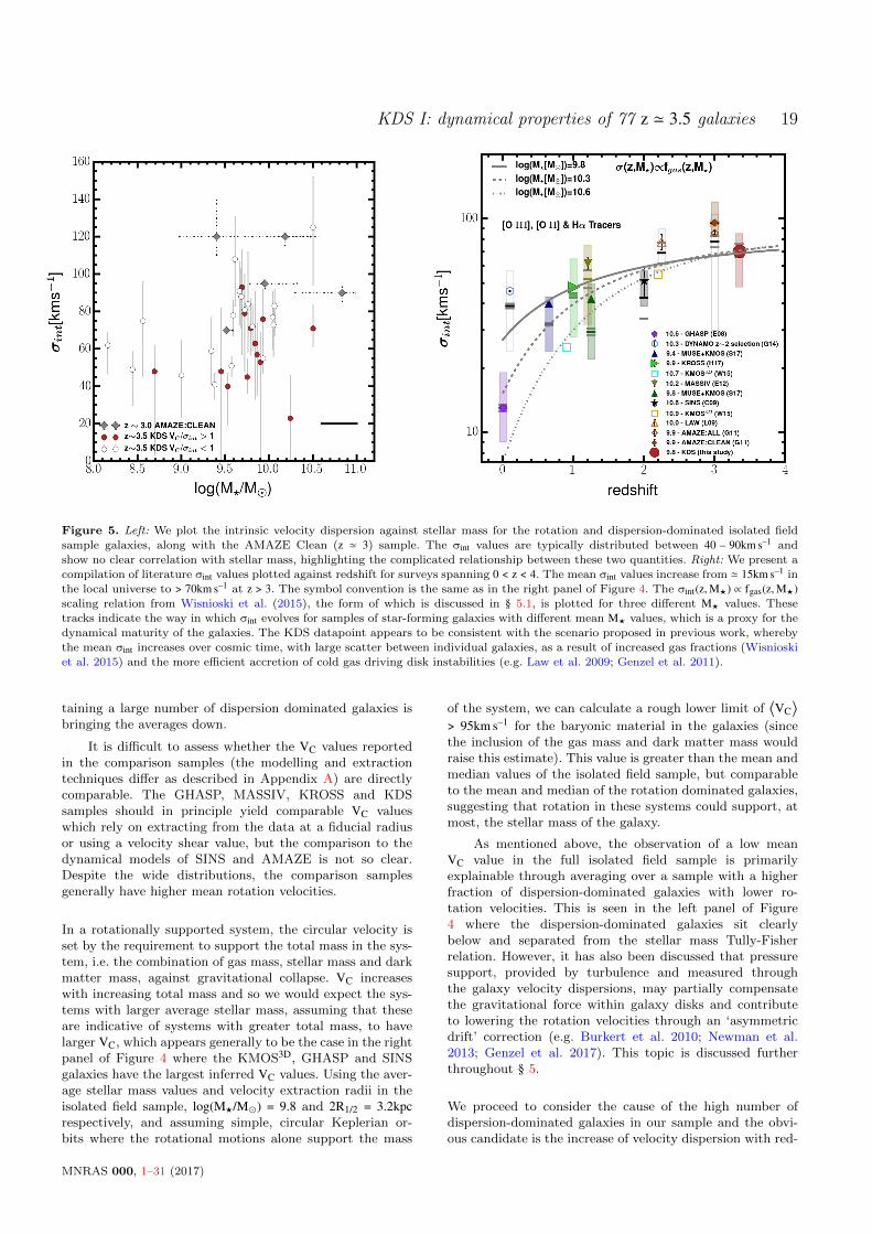
KDS I: dynamical properties of 77 z ' 3.5 galaxies 19

Figure 5. Left: We plot the intrinsic velocity dispersion against stellar mass for the rotation and dispersion-dominated isolated field

sample galaxies, along with the AMAZE Clean (z ' 3) sample. The σint values are typically distributed between 40 – 90km s–1 andshow no clear correlation with stellar mass, highlighting the complicated relationship between these two quantities. Right: We present a

compilation of literature σint values plotted against redshift for surveys spanning 0 < z < 4. The mean σint values increase from ' 15km s–1 inthe local universe to > 70km s–1 at z > 3. The symbol convention is the same as in the right panel of Figure 4. The σint(z,M?) ∝ fgas(z,M?)scaling relation from Wisnioski et al. (2015), the form of which is discussed in § 5.1, is plotted for three different M? values. These

tracks indicate the way in which σint evolves for samples of star-forming galaxies with different mean M? values, which is a proxy for thedynamical maturity of the galaxies. The KDS datapoint appears to be consistent with the scenario proposed in previous work, whereby

the mean σint increases over cosmic time, with large scatter between individual galaxies, as a result of increased gas fractions (Wisnioski

et al. 2015) and the more efficient accretion of cold gas driving disk instabilities (e.g. Law et al. 2009; Genzel et al. 2011).

taining a large number of dispersion dominated galaxies isbringing the averages down.

It is difficult to assess whether the VC values reportedin the comparison samples (the modelling and extractiontechniques differ as described in Appendix A) are directlycomparable. The GHASP, MASSIV, KROSS and KDSsamples should in principle yield comparable VC valueswhich rely on extracting from the data at a fiducial radiusor using a velocity shear value, but the comparison to thedynamical models of SINS and AMAZE is not so clear.Despite the wide distributions, the comparison samplesgenerally have higher mean rotation velocities.

In a rotationally supported system, the circular velocity isset by the requirement to support the total mass in the sys-tem, i.e. the combination of gas mass, stellar mass and darkmatter mass, against gravitational collapse. VC increaseswith increasing total mass and so we would expect the sys-tems with larger average stellar mass, assuming that theseare indicative of systems with greater total mass, to havelarger VC, which appears generally to be the case in the rightpanel of Figure 4 where the KMOS3D, GHASP and SINSgalaxies have the largest inferred VC values. Using the aver-age stellar mass values and velocity extraction radii in theisolated field sample, log(M?/M�) = 9.8 and 2R1/2 = 3.2kpcrespectively, and assuming simple, circular Keplerian or-bits where the rotational motions alone support the mass

of the system, we can calculate a rough lower limit of⟨VC

⟩> 95km s–1 for the baryonic material in the galaxies (sincethe inclusion of the gas mass and dark matter mass wouldraise this estimate). This value is greater than the mean andmedian values of the isolated field sample, but comparableto the mean and median of the rotation dominated galaxies,suggesting that rotation in these systems could support, atmost, the stellar mass of the galaxy.

As mentioned above, the observation of a low meanVC value in the full isolated field sample is primarilyexplainable through averaging over a sample with a higherfraction of dispersion-dominated galaxies with lower ro-tation velocities. This is seen in the left panel of Figure4 where the dispersion-dominated galaxies sit clearlybelow and separated from the stellar mass Tully-Fisherrelation. However, it has also been discussed that pressuresupport, provided by turbulence and measured throughthe galaxy velocity dispersions, may partially compensatethe gravitational force within galaxy disks and contributeto lowering the rotation velocities through an ‘asymmetricdrift’ correction (e.g. Burkert et al. 2010; Newman et al.2013; Genzel et al. 2017). This topic is discussed furtherthroughout § 5.

We proceed to consider the cause of the high number ofdispersion-dominated galaxies in our sample and the obvi-ous candidate is the increase of velocity dispersion with red-

MNRAS 000, 1–31 (2017)

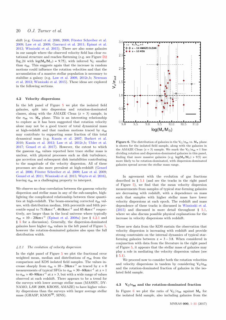
20 O.J. Turner et al.

shift (e.g. Genzel et al. 2006, 2008; Forster Schreiber et al.2009; Law et al. 2009; Gnerucci et al. 2011; Epinat et al.2012; Wisnioski et al. 2015). There are also some galaxiesin our sample where the observed velocity field has clear ro-tational structure and reaches flattening (e.g. see Figure D2lbg 24 with log(M?/M�) = 9.75), with inferred VC smallerthan σint. This suggests again that the increase in randommotions could influence the rotation velocities and that theaccumulation of a massive stellar population is necessary tostabilise a galaxy (e.g. Law et al. 2009, 2012c,b; Newmanet al. 2013; Wisnioski et al. 2015). These ideas are exploredin the following sections.

4.2 Velocity dispersions

In the left panel of Figure 5 we plot the isolated fieldgalaxies, split into dispersion and rotation-dominatedclasses, along with the AMAZE Clean (z ' 3) sample, inthe σint vs. M? plane. This is an interesting relationshipto explore as it has been suggested that rotation velocityalone may not be a good tracer of total dynamical massat high-redshift and that random motions traced by σintmay contribute to supporting some fraction of this totaldynamical mass (e.g. Kassin et al. 2007; Burkert et al.2010; Kassin et al. 2012; Law et al. 2012c,b; Ubler et al.2017; Genzel et al. 2017). However, the extent to whichthe gaseous σint values reported here trace stellar mass isunclear, with physical processes such as disk turbulence,gas accretion and subsequent disk instabilities contributingto the magnitude of the velocity dispersion. All of theseprocesses are also more prevalent at high-redshift (Genzelet al. 2006; Forster Schreiber et al. 2009; Law et al. 2009;Genzel et al. 2011; Wisnioski et al. 2015; Wuyts et al. 2016),leaving σint as a challenging property to interpret.

We observe no clear correlation between the gaseous velocitydispersion and stellar mass in any of the sub-samples, high-lighting the complicated relationship between these quanti-ties at high-redshift. The beam-smearing corrected σint val-ues, with distribution median, 16th percentile and 84th per-centile equal to 71.0km s–1, 48.0km s–1 and 85.4km s–1 respec-tively, are larger than in the local universe where typicallyσint = 10 – 20km s–1 (Epinat et al. 2008a) (see § 4.2.1 and§ 5 for a discussion). Generally, the dispersion-dominatedgalaxies have higher σint values in the left panel of Figure 5,however the rotation-dominated galaxies also span the fulldistribution width.

4.2.1 The evolution of velocity dispersion

In the right panel of Figure 5 we plot the fractional errorweighted mean, median and distributions of σint from thecomparison and KDS isolated field samples. The values in-crease sharply from σint ' 10 – 20km s–1 as traced by z ' 0measurements of typical SFGs to σint ' 30–60km s–1 at z ' 1to σint ' 40–90km s–1 at z ' 3, but with a wide range of valuesobserved at each redshift. There appears to be a trend forthe surveys with lower average stellar mass (MASSIV, DY-NAMO, LAW 2009, KROSS, AMAZE) to have higher veloc-ity dispersions than the surveys with larger average stellarmass (GHASP, KMOS3D, SINS).

Figure 6. The distribution of galaxies in the VC/σint vs. M? planeis shown for the isolated field sample, along with the galaxies in

the AMAZE Clean (z ' 3) sample. We mark the VC/σint = 1 line

dividing rotation and dispersion-dominated galaxies in this panel,finding that more massive galaxies (e.g. log(M?/M�) > 9.5) are

more likely to be rotation-dominated, with dispersion-dominated

galaxies spread across the stellar mass range.

In agreement with the evolution of gas fractionsdescribed in § 5.1 (and see the tracks in the right panelof Figure 5), we find that the mean velocity dispersionmeasurements from samples of typical star-forming galaxiesare decreasing with redshift, with a dependence on masssuch that samples with higher stellar mass have lowervelocity dispersions at each epoch. The redshift and massdependence of these tracks is discussed in Wisnioski et al.(2015) and discussed in more detail throughout § 5.1,where we also discuss possible physical explanations for theincrease in velocity dispersions with redshift.

These new data from the KDS sustain the observation thatvelocity dispersion is increasing with redshift and providestrong constraints on the internal dynamics of typical star-forming galaxies between z = 3 – 3.8. When considered inconjunction with data from the literature in the right panelof Figure 5, it appears that the stellar mass of galaxies mayplay a role in mediating the velocity dispersion values (see§ 5.1).

We proceed now to consider both the rotation velocitiesand velocity dispersions in tandem by considering VC/σintand the rotation-dominated fraction of galaxies in the iso-lated field sample.

4.3 VC/σint and the rotation-dominated fraction

In Figure 6 we plot the ratio of VC/σint against M? forthe isolated field sample, also including galaxies from the

MNRAS 000, 1–31 (2017)

KDS I: dynamical properties of 77 z ' 3.5 galaxies 21

Figure 7. Left: VC/σint is plotted against redshift for the comparison samples spanning 0 < z < 4. We see a clear decline in the mean VC/σintvalues with redshift, but with wide ranges in the individual measurements. There is a connection between VC/σint and the stellar massof the surveys, with larger mean M? surveys reporting higher mean VC/σint. Right: We plot the associated rotation-dominated fraction,

defined as the fraction of galaxies in each sample with VC/σint > 1. The narrow shaded regions represent the maximum and miminumRDF, computed as described in Appendix A. It appears that the rotation-dominated fraction drops from ' 100% in the local universe

to 60% at intermediate redshifts and then to ' 35% at z ' 3.5, again with the trend for high VC/σint values in the larger M? surveys

reflected by higher rotation-dominated fractions. The dot-dash line is the RDF ∝ z–0.2 cosmic decline suggested in Stott et al. (2016),which appears to follow the redshift decline of the rotation dominated fraction. In both panels, the symbol convention is the same as in

the right panel of Figure 4.

AMAZE Clean (z ' 3) sample for reference. In the localuniverse, disky, SFGs are observed to have VC/σint valuesin excess of 10 (i.e. the disks are ‘well settled’), due tothe decline of velocity dispersion across cosmic time, asgas fractions and disk turbulence decrease (e.g. Epinatet al. 2008a,b). Clearly the isolated field sample galaxiesare in a different physical regime, with mean and medianVC/σint values of 1.08+0.18–0.15 and 0.97+0.14–0.11 respectively. This isdespite many of the dispersion-dominated galaxies showingclear velocity gradients across the observed velocity maps(Appendix D), with the arctangent model providing a goodfit to the rotation curves. This suggests that althoughrotational motions are present within the disks, they aresmall or comparable with the elevated σint values observedthroughout the z ' 3.5 sample.

The VC/σint = 1 line dividing rotation and dispersion-dominated galaxies is marked on Figure 6, separating thedispersion and rotation-dominated galaxies by definition.There is a spread of rotation and dispersion-dominatedgalaxies across the stellar mass range, with rotation-dominated galaxies more likely to be found abovelog(M?/M�) > 9.5. The Rotation-Dominated Fraction(RDF), calculated with respect to the full field sampleof 38 galaxies, is 0.34±0.08, which is substantially lowerthan in the local and intermediate redshift universe (e.g.Epinat et al. 2008a,b; Green et al. 2014). We interpret theseresults in the context of the cosmic evolution of the rotation

dominated fraction using the comparison samples in § 4.3.1.

4.3.1 The evolution of the rotation-dominated fraction

In the left and right panels of Figure 7 we plot VC/σintand the closely connected rotation-dominated fractionrespectively as a function of redshift for the KDS isolatedfield sample and the comparison samples described in Ap-pendix A. In each sample, the rotation dominated fractionis computed as the fraction of galaxies with VC/σint > 1,which, given the varying data quality across the comparisonsamples, is a simple and fair way to study the redshiftevolution of this quantity. The filled and hollow symbolswith black errorbars in the left panel of Figure 7 representthe mean and error on the mean, and the horizontal linesshow the median and error on the median. The shadedregions give the 16th and 84th percentiles of the distributionof individual VC/σint measurements, plotted here to indicatethe range of measurements at each redshift slice. In the rightpanel of Figure 7, we have also computed the maximum andminimum RDF for these surveys by adding and subtractingthe VC/σint error values respectively and recomputing therotation-dominated fraction. These are shown with the thingrey shaded regions and are intended to give an indicationof the limits of the RDF at different redshift slices giventhe size of the errors on the individual points.

MNRAS 000, 1–31 (2017)

22 O.J. Turner et al.

The rotation-dominated fraction, traced simply by theVC/σint ratio inferred from ionised gas emission lines, dropsfrom ' 100% of galaxies in the local universe to ' 2/3of galaxies in the z ' 1 – 2 universe and to ' 1/3 abovez ' 3, albeit with individual surveys reporting wide VC/σintdistributions at each redshift slice. This is highlightedin the right panel of Figure 7 by overplotting the RDF∝ z–0.2 line which appears to roughly follow the declineof the rotation-dominated with redshift as described inStott et al. (2016). The width of the VC/σint distributionsindicate the galaxy diversity at each redshift slice, drivenby the collection of galaxy masses, sSFRs, gas fractions,morphologies and evolutionary states which compriseeach sample. Scatter above and below the RDF ∝ z–0.2evolution line may be attributed in part to the differentmean stellar masses of the surveys, with those that havelarger stellar masses tending to scatter above this line.This draws again from the idea that higher stellar massvalues suggest that the galaxies are more evolved, withmore gas having been converted into stars for the bulk ofthe sample, which provides stability for a rotating diskand pushes the rotation-dominated fraction higher (see § 5).

In summary, the rotation-dominated galaxies in theisolated field sample appear to conform with a redshiftinvariant VC - M? relation. Due to increased velocitydispersions, these rotation-dominated galaxies account foronly 34% of the field sample and so are less representative oftypical star-forming galaxies at z ' 3.5 than at intermediateand low redshifts. Explanations for the increase of σint withredshift (and hence the decline of VC/σint) with cosmictime as well as the nature of dispersion-dominated galaxieshave been discussed at length throughout other studies (e.gForster Schreiber et al. 2009; Law et al. 2009; Burkert et al.2010; Newman et al. 2013; Wisnioski et al. 2015) and werevisit these in the following discussion.

5 DISCUSSION

Throughout § 4 we have investigated the derived kinematicparameters of the isolated field sample, showing first that,within the scatter, the rotation-dominated galaxies sit on arotation velocity - stellar mass relationship consistent withwhat is observed in the local universe. The mean rota-tion velocity of the isolated field sample is low as a re-sult of averaging over a sample containing a large num-ber of dispersion-dominated galaxies (66% of the sample)and probable pressure support from turbulent motions (e.g.Burkert et al. 2010). This increased number of dispersion-dominated galaxies in comparison to low and intermediateredshifts appears to be driven by high velocity dispersions atz ' 3.5. In this section we discuss possible physical originsfor the elevated random motions traced by σint and theirimpact on the galactic dynamics.

5.1 The origin and impact of increased velocitydispersions at high-redshift

Previous studies have claimed that the elevated velocity dis-persions observed at high-redshift are a consequence of bothinternal and external processes. Law et al. (2009) observe

galaxies with elevated velocity dispersions at z ' 2.2 (seeFigure 5) and attribute this to gravitational instabilities fol-lowing efficient accretion, which can occur when the cold gasbecomes dynamically dominant.

Genzel et al. (2011) show that for dispersion-dominatedgalaxies, the scales susceptible to gravitational collapse areof the order of the galactic half-light radius. Systems such asthese form highly unstable and roughly spherical stellar dis-tributions with large internal motions at early times, beforemore gradual accretion from the galactic halo forms an ex-tended, stable, gaseous disk which instigates kinematic order(Law et al. 2009; Genzel et al. 2011). The physical mecha-nisms responsible for the increase in σint may also result ina reduction in the observed rotation velocities by partiallycompensating the gravitational force throughout the galacticdisk (e.g. Burkert et al. 2010; Wuyts et al. 2016; Ubler et al.2017; Genzel et al. 2017; Lang et al. 2017). Following this,σint decreases over time as ordered rotation begins to domi-nate and pressure support becomes increasingly insignificant(e.g. Burkert et al. 2010; Ubler et al. 2017; Genzel et al. 2017;Lang et al. 2017). This is in line with the evolution of gasfractions observed at intermediate and high-redshifts (e.g.Saintonge et al. 2013; Tacconi et al. 2013, 2017), with thegas reservoirs of galaxies fed by the accretion of cold gas.Burkert et al. (2010) show, starting from the hydrostaticequation, that negative pressure gradients sourced by thedisk turbulence generated through gravitational instabilitiesresult in a decrease in observed rotation velocities. Thishas prompted others (e.g. Wuyts et al. 2016; Ubler et al.2017; Lang et al. 2017) to encorporate a velocity dispersionterm in the derivation of maximum circular velocities,which contributes to (but is not entirely responsible for)the observed shift in the zero-point of the stellar massTully-Fisher relation between z ' 0 – 0.9. Ubler et al.(2017) also claim that without the inclusion of this termincorrect conclusions surrounding the evolution of theTully-Fisher relation will be drawn. We have not encor-porated such a term when deriving the rotation velocitiesof the isolated field sample, but note that as a conse-quence of our galaxies showing some of the most extremeintrinsic dispersions observed, this would undoubtedlylead to a different distribution in the VC – M? plane.The contribution of pressure to rotation velocity for theKDS sample will be explored in more detail in a future work.

In Wisnioski et al. (2015) the authors present a scaling rela-tion describing the increase of σint with redshift in terms ofthe key observable properties: gas fraction, fgas, gas deple-tion timescale, tdep, and specific star-formation rate, sSFR.Here we explore how well this model describes the evolu-tion in velocity dispersion, incorporating our new measure-ment at z ' 3.5 from the KDS. The function describing theevolution of the velocity dispersion with redshift is shownbelow in Equation 10, where Qcrit is the critical Toomre pa-rameter for stability against gravitational collapse (Toomre1964), and a is a dimensionless parameter which depends onthe assumed distribution of gas and gravitational potentialForster Schreiber et al. (2006).

σ(z,M?) =VCQcrit

afgas(z,M?) (10)

The gas fraction is a function of gas depletion timescale, with

MNRAS 000, 1–31 (2017)

KDS I: dynamical properties of 77 z ' 3.5 galaxies 23

Figure 8. Left: We plot the σint values for the comparison samples as well as the isolated field sample, shifted as described in the text

to a reference mass of log(M?/M�) = 9.8 (the median mass of the isolated field sample). The grey line shows the model prediction withVCQcrit/a = 90.5km s–1, as dictated by our data. The grey shaded region encompasses the model predictions with lower and upper bounds

using VCQcrit/a = 50 – 140km s–1 respectively (corresponding roughly to the velocity range VC = 70 – 200km s–1, spanned by galaxies in thecomparison samples, under the assumption that Qcrit = 1.0 and a =

√2 as discussed in the text). The shifted points are in line with the

scenario whereby the sample averaged velocity dispersions increase with redshift as a result of increasing average gas fractions. Right:

The same as in the left panel for a reference mass of log(M?/M�) = 10.6. The steeper slope beyond z ' 2 highlights the model decrease ingas fraction, and hence velocity dispersion, for galaxies which have accumulated a larger stellar population.

an assumed redshift dependence, and specific star-formationrate, with an assumed mass and redshift dependence (seeWisnioski et al. 2015 Equations 3-6, summarised below byEquations 11 and 12).

fgas =1

1 +(tdepsSFR

)–1=

11 +

(1.5 × 10a(M?)(1 + z)b(M?)+α

)–1 (11)

a(M?) = –10.73 +1.26

1 + e(10.49–log(M?/M�))/(–0.25)

b(M?) = 1.85 +1.57

1 + e(10.35–log(M?/M�))/(0.19)

(12)

This relation is an expression of the belief that high-redshiftgalaxies experience more intense and efficient gas inflow,with the accumulation of a more massive stellar popula-tion providing stability against perturbations. In this equi-librium model framework (e.g. Dave et al. 2012; Lilly et al.2013; Saintonge et al. 2013), populations of disk galaxieswith higher average stellar mass have lower average velocitydispersions due to this stability condition.

In the right panel of Figure 5 we plot Equa-tion 10 for three different input mass values(log(M?/M�) = 9.8, 10.3, 10.6, roughly spanning the massrange of the comparison samples), using the updateddepletion time scaling relation from Tacconi et al. (2017)

(i.e. tdep ∝ (1 + z)–0.57, meaning α = 0.57 in Equation 11). TheEquation σ(z,M?) ∝ fgas(z,M?) is scaled so that the lowestmass track conincides with the KDS datapoint, finding aproportionality constant VCQcrit/a = 90.5km s–1, which weassume when plotting all three tracks in Figure 5.

In this model, the velocity dispersions increase more steeplywith increasing stellar mass, as shown by the solid anddashed lines in Figure 5. At higher redshift, these lines con-verge, suggesting that the predictions for the gas fractionbecome independent of stellar mass in this regime. In gen-eral, the surveys with higher stellar mass have lower velocitydispersions, in support of the model hypothesis.

Since stellar mass appears to be a crucial factor in regu-lating the velocity dispersions within galaxies, and the com-parison samples have disparate stellar mass ranges, we usethe model to shift the σint values according to their stellarmass to a reference mass value as per Wisnioski et al. (2015).This is done by computing the difference between the modelpredicted σint value at the stellar mass of each comparisonsurvey, and at the reference mass for the appropriate red-shift, and shifting the reported σint by this value. We do thisfor two reference mass values; log(M?/M�) = 9.8 (the medianmass of the isolated field sample, left panel of Figure 8) andlog(M?/M�) = 10.6 (right panel of Figure 8).

In both panels, the solid grey line denotes the modelprediction using the parameter combination determinedabove; VCQcrit/a = 90.5km s–1. The grey shaded regionsencompass model predictions with lower and upper bounds

MNRAS 000, 1–31 (2017)

24 O.J. Turner et al.

defined by VCQcrit/a = 50 – 140km s–1 respectively. Assumingthat Qcrit = 1.0 (as for a quasi-stable thin disk e.g. Forster

Schreiber et al. 2006; Burkert et al. 2010) and a =√2 (as for

a disk with constant rotation velocity Wisnioski et al. 2015),this range corresponds to VC = 70 – 200km s–1, which isroughly the velocity range spanned by our comparison sam-ples, and the solid grey line corresponds to VC = 128km s–1.Whilst the KDS mean rotation velocity sits at the bottomof this range, possible explanations are: (1) The rotationvelocities of the KDS galaxies are underestimated as aresult of the velocity dispersion contribution discussedabove; (2) Qcrit , 1 or a ,

√2 as a consequence of changing

physical conditions at high-redshift.

Although the details of the coefficients of Equation 10 areunclear (i.e. VC is not fixed at one value for the comparisonsamples and is itself linked to stellar mass, and both Qcrit anda could vary with redshift), the shape of the velocity disper-sion evolution appears to follow that of the gas fraction, assuggested by the model. The difference between the slopes inthe left and right panels highlights the role of stellar mass inthe kinematic settling of galaxies between z ' 3 and the localuniverse. The isolated field sample data, in combination withcomparison sample results spanning z = 0 – 3, thus suggestthat the time evolution of the velocity dispersion measuredfrom ionised gas emission lines is intimately linked to theconsumption of gas and the accumulation of stars in a stabledisk (e.g. Law et al. 2009, 2012c,b; Wisnioski et al. 2015).Rotation-dominated galaxies become less representative ofthe typical star-forming population at these redshifts as aresult of the increased velocity dispersions (shown in Figure7), constituting only ' 1/3 of the isolated field sample atz ' 3.5. This suggests that we are probing more chaotic andunstable systems, subject to gravitational instabilities andcollapse on the disk scale length (Burkert et al. 2010; Gen-zel et al. 2011), residing in a much more active period of theuniverse in terms of both accretion and star-formation. Re-cent results indicate that these systems may become stronglybaryon-dominated on the galaxy disk scale at high-redshift(Ubler et al. 2017; Lang et al. 2017; Genzel et al. 2017),which could imply that the increasing contribution of darkmatter to galaxy disks with decreasing redshift plays a rolein the evolution of velocity dispersions.

The precise interpretation of the velocity dispersion re-mains unclear, although there is mounting evidence that ran-dom motions have an increasingly significant contribution tothe mass budget of high-redshift galaxies (e.g. Kassin et al.2007; Law et al. 2009; Burkert et al. 2010; Kassin et al. 2012;Wuyts et al. 2016; Lang et al. 2017; Ubler et al. 2017; Genzelet al. 2017). The nature of dispersion-dominated galaxies athigh-redshift has been discussed in Newman et al. (2013) us-ing Adaptive-Optics (AO) and seeing limited observations ofthe same galaxies. The AO observations show that, in somecases, galaxies which are clasified as dispersion-dominatedwith seeing limited observations reveal much larger velocitygradients at higher spatial resolution. This highlights thatbeam-smearing effects can wash-out observed rotational mo-tions, particularly for small galaxies. We have attempted toaccount for beam-smearing using half-light radius and ve-locity gradient dependent dynamical modelling, but we ac-knowledge that these observations are challenging and can-not rule out the presence of unresolved velocity gradients in

our seeing-limited dataset. Smaller galaxies do have intrinsi-cally smaller rotation velocities, whilst there is no observeddependence of velocity dispersion on galaxy size (e.g. New-man et al. 2013). Dispersion-dominated galaxies are there-fore likely to be at an earlier evolutionary stage and unsta-ble to gravitational instabilities which generate turbulencewhich is then maintained by the potential energy of the gasin the disk (Burkert et al. 2010; Newman et al. 2013).

Bringing the above points together, turbulent motionsconsume an increasingly significant fraction of the energybudget at high-redshift when typical star-forming galax-ies are at earlier evolutionary stages. The KDS isolatedfield sample presents an extension of these trends tohigher redshift, where galaxies are even more likely to bedispersion-dominated, and pressure support may be moresignificant than explored at z ' 2.3 (Wuyts et al. 2016; Ubleret al. 2017; Genzel et al. 2017; Lang et al. 2017). However,the precise interpretation of σint measured from ionised gasemission lines remains unclear, and future observations ofboth stellar and gaseous velocity dispersions in tandemwith JWST will allow for unambigous investigations intothe nature of gaseous velocity dispersions at high-redshift.

In summary, the isolated field sample galaxies are diverseand kinematically immature, with ' 2/3 of the sample be-ing dominated by random motions which may contributeto supporting a portion of the dynamical mass (e.g. Kassinet al. 2007; Burkert et al. 2010; Kassin et al. 2012; New-man et al. 2013; Straatman et al. 2017; Ubler et al. 2017;Lang et al. 2017). In the context of the equilibrium modelexplored here, these galaxies will evolve gradually with red-shift along the velocity-mass relationship into stable diskgalaxies which have converted their gas reservoirs into stel-lar mass (e.g. Lilly et al. 2013; Tacconi et al. 2013; Wisnioskiet al. 2015; Tacconi et al. 2017). Future work at higher reso-lution and redshift will trace the extent to which gas-derivedvelocity dispersions trace the stellar dispersions and will in-vestigate even earlier and more chaotic stages in the lifetimesof late-type galaxies.

6 CONCLUSIONS

We have presented new dynamical measurements of 32 typ-ical star-forming galaxies spanning both cluster and fieldenvironments at z ' 3.5 as part of the KMOS Deep Survey,based on IFU data observed with KMOS. These measure-ments push back the frontier of IFU observations in the earlyuniverse and provide more robust constraints on the internaland rotational dynamics of 9.0 < log(M?/M�) < 10.5 typicalstar-forming galaxies at these redshifts. By using a com-bined morpho-kinematic classification based on broad-bandHST imaging and our IFU data, we have separated inter-acting galaxies from the sample, finding merger rates con-sistent between the field pointings (' 16%) and a very highmerger rate in the cluster pointing (' 89%). We have madebeam-smearing corrected measurements of VC and σint forthe remaining isolated field galaxies, and we interpret thesein the context of previous dynamical studies using IFU data(Appendix A and Table A1). The main conclusions of thiswork are summarised as follows:

• We use a fractional error weighted mean to derive the mean

MNRAS 000, 1–31 (2017)

KDS I: dynamical properties of 77 z ' 3.5 galaxies 25

kinematic parameters of the KDS isolated field sample ofVC = 76.7+4.9–4.5km s–1 and σint = 70.8+3.3–3.1km s–1 (right panels ofFigures 4 and 5 respectively). Rotation (dispersion) domi-nated galaxies are defined as those with VC/σint > (<)1.

• We plot the mean VC values of the comparison samples andthe KDS isolated field sample, finding significant diversityin VC measurements in each survey (right panel of Figure4). The spread in measurements is a result of the samplescontaining a mixture of rotation and dispersion-dominatedgalaxies with varying M? values, and the low mean KDSvalue is primarily the result of averaging over a sample witha high fraction of dispersion-dominated galaxies and indi-cating the impact pressure support may have on reducingrotation velocities. At higher M?, the accumulation of a stel-lar population provides stability, leading to an interplay be-tween σint and VC mediated across redshift by the cosmicdecline of gas fractions, sSFRs and accretion (e.g. Law et al.2012c; Wisnioski et al. 2015).

• When the VC values are viewed as a function of mass inthe inverse stellar mass Tully-Fisher Relation, the rotation-dominated galaxies are correlated with mass and lie withinthe errors on the same relation as derived for rotation-dominated galaxies with 9.0 < log(M?/M�) < 11.0 at z ' 0.9in the KROSS survey (Figure 4). This relation is consistentwith star-forming galaxies at z = 0 and so we report no sig-nificant evolution in the slope or zero-point of the smTFRbetween z = 0 – 3.5. Consistency of sample selection andmeasurement techniques are crucial factors when determin-ing evolution in the VC vs. M? plane by comparing samplesat different redshifts. The dispersion-dominated galaxies inthe isolated field sample scatter below the trend.

• When considering the rotation-dominated galaxies alone,the mean and median rotation velocities are VC =96.7+7.3–7.2km s–1 and VC = 93.0+12.0–12.5km s–1 respectively, whichare roughly equivalent to a simple lower limit virial theoremcalculation using the mean mass and half-light radius of thesample. This suggests that pressure forces, which are moresignificant at high-redshift, may play a role in supporting thetotal mass in all of the galaxies in the isolated field sample(e.g. Burkert et al. 2010).

• 13/32 isolated field sample galaxies are rotation-dominatedand 19/32 are dispersion-dominated, with a tendency forgalaxies with higher M? to have larger values of VC/σint (Fig-ure 6). This gives a rotation-dominated fraction of 34 ± 8%in the isolated field sample, substantially less than sur-veys at lower redshift, although there is significant diversityamongst the individual VC/σint measurements at each red-shift slice (left and right panels of Figure 7). When viewedas a function of redshift, the rotation dominated fractionappears to follow the scaling relation RDF∝ z–0.2.• We plot mean σint values computed in a consistent way forSFG samples spanning a wide redshift baseline (the com-parison samples described in Appendix A), finding a sharpincrease in σint values between z = 0 – 1 and a fairly shallowincrease thereafter, mediated by the mean M? of the galaxysamples (right panel of Figure 5). This is in line with a sim-ple equilibrium model prescription in which the gas fractionsand the impact of several physical mechanisms such as ac-cretion of gas from the IGM, stellar feedback and turbulenceincrease with redshift and combine to increase random mo-tions within high-redshift galaxies.

ACKNOWLEDGEMENTS

OJT acknowledges the financial support of the Scienceand Technology Facilities Council through a studentshipaward. MC and OJT acknowledge the KMOS team andall the personnel of the European Southern ObservatoryVery Large Telescope for outstanding support during theKMOS GTO observations. CMH, AMS and RMS acknowl-edge the Science and Technology Facilities Council throughgrant code ST/L00075X/1. RJM acknowledges the supportof the European Research Council via the award of a Con-solidator Grant (PI: McLure). JSD acknowledges the sup-port of the European Research Council via the award ofan Advanced Grant (PI J. Dunlop), and the contributionof the EC FP7 SPACE project ASTRODEEP (Ref.No:312725). AMS acknowledges the Leverhulme Foundation.JM acknowledges the support of a Huygens PhD fellowshipfrom Leiden University. DS acknowledges financial supportfrom the Netherlands Organization for Scientific research(NWO) through a Veni fellowship and from FCT throughan FCT Investigator Starting Grant and Start-up Grant(IF/01154/2012/CP0189/CT0010). This work is based onobservations taken by the CANDELS Multi-Cycle TreasuryProgram with the NASA/ESA HST, which is operated bythe Association of Universities for Research in Astronomy,Inc., under NASA contract NAS5-26555. This work is basedon observations taken by the 3D-HST Treasury Program(GO 12177 and 12328) with the NASA/ESA HST, which isoperated by the Association of Universities for Research inAstronomy, Inc., under NASA contract NAS5-26555. Basedon data obtained with the European Southern ObservatoryVery Large Telescope, Paranal, Chile, under Large Program185.A-0791, and made available by the VUDS team at theCESAM data center, Laboratoire d’Astrophysique de Mar-seille, France.

MNRAS 000, 1–31 (2017)

26 O.J. Turner et al.

REFERENCES

Abramson L. E., Gladders M. D., Dressler A., Oemler A., Pog-

gianti B., Vulcani B., 2016, ApJ, 832, 7

Balestra I., et al., 2010, A&A, 512, A12

Barrera-Ballesteros J. K., et al., 2014, A&A, 568, A70

Barrera-Ballesteros J. K., et al., 2015, A&A, 582, A21

Behroozi P. S., Wechsler R. H., Conroy C., 2013, ApJ, 770, 57

Bell E. F., de Jong R. S., 2001, ApJ, 550, 212

Bell E. F., et al., 2004, ApJ, 608, 752

Bertin E., Arnouts S., 1996, A&AS, 117, 393

Bouche N., Carfantan H., Schroetter I., Michel-Dansac L., Contini

T., 2015, AJ, 150, 92

Bournaud F., Frederic 2016, Ap&SS, 418, 355

Bournaud F., Elmegreen B. G., Elmegreen D. M., 2007, ApJ, 670,

237

Brammer G. B., et al., 2011, ApJ, 739, 24

Brammer G. B., et al., 2012, ApJS, 200, 13

Brown M. J. I., Dey A., Jannuzi B. T., Brand K., Benson A. J.,

Brodwin M., Croton D. J., Eisenhardt P. R., 2007, ApJ, 654,858

Bruce V. A., et al., 2012, MNRAS, 427, 1666

Bruzual G., Charlot S., 2003, MNRAS, 344, 1000

Buitrago F., Trujillo I., Conselice C. J., Haeussler B., 2013, MN-

RAS, 428, 1460

Bundy K., et al., 2015, ApJ, 798, 7

Burkert A., et al., 2010, ApJ, 725, 2324

Calzetti D., Armus L., Bohlin R., 2000, ApJ, 20, 682

Cappellari M., et al., 2011, MNRAS, 413, 813

Cassata P., et al., 2015, A&A, 573, A24

Conselice C. J., 2014, ARA&A, 52, 291

Conselice C. J., et al., 2011, MNRAS, 413, 80

Contini T., et al., 2016, A&A, 591, A49

Courteau S., 1997, AJ, p. 6

Cresci G., et al., 2009, ApJ, 697, 115

Cresci G., Mannucci F., Maiolino R., Marconi a., Gnerucci a.,Magrini L., 2010, Nature, 467, 811

Croom S. M., et al., 2012, MNRAS, 421, 872

Cullen F., Cirasuolo M., McLure R. J., Dunlop J. S., Bowler R.

a. a., 2014, MNRAS, 440, 2300

Daddi E., et al., 2007, ApJ, 670, 156

Darvish B., Mobasher B., Sobral D., Rettura A., Scoville N.,Faisst A., Capak P., 2016, ApJ, 825, 113

Dave R., Finlator K., Oppenheimer B. D., 2012, MNRAS, 421,

98

Davies R. I., 2007, MNRAS, 375, 1099

Davies R., et al., 2011, ApJ, 741, 69

Davies R. I., et al., 2013, ApJ, 558, A56

Dekel A., Birnboim Y., 2006, MNRAS, 368, 2

Di Teodoro E., Fraternali F., 2015, MNRAS, 451, 3021

Di Teodoro E. M., Fraternali F., Miller S. H., 2016, A&A, 594,A77

Dubois Y., et al., 2014, MNRAS, 444, 1453

Elbaz D., et al., 2007, A&A, 468, 33

Elmegreen D. M., Elmegreen B. G., Sheets C. M., 2004, ApJ, 603,

74

Epinat B., et al., 2008a, MNRAS, 388, 500

Epinat B., Amram P., Marcelin M., 2008b, MNRAS, 390, 466

Epinat B., Amram P., Balkowski C., Marcelin M., 2010, MNRAS,401, 2113

Epinat B., et al., 2012, A&A, 539, A92

Faber S. M., et al., 2007, ApJ, 665, 265

Fall S. M., 1983, IN: Internal kinematics and dynamics of galaxies;

Proceedings of the Symposium, Besancon, France, August 9-13, 1982 (A83-49201 24-89). Dordrecht, D. Reidel PublishingCo., 1983, p. 391-398; Discussion, 399., 100, 391

Fall S. M., Romanowsky A. J., 2013, ApJL, 769, L26

Flores H., Hammer F., Puech M., Amram P., Balkowski C., 2006,

A&A, 455, 107

Foreman-Mackey D., Hogg D. W., Lang D., Goodman J., 2013,PASP, 125, 306

Forster Schreiber N. M., et al., 2006, ApJ, 645, 1062

Forster Schreiber N. M., et al., 2009, ApJ, 706, 1364

Freudling W., Romaniello M., Bramich D. M., Ballester P., Forchi

V., Garcia-Dablo C. E., Moehler S., Neeser M. J., 2013, A&A,559, A96

Genzel R., et al., 2006, Nature, 442, 786

Genzel R., et al., 2008, ApJ, 687, 59

Genzel R., et al., 2011, ApJ, 733, 101

Genzel R., et al., 2017, Nature, 543, 397

Gladders M. D., Oemler A., Dressler A., Poggianti B., Vulcani

B., Abramson L., 2013, ApJ, 770, 64

Gnerucci A., et al., 2011, A&A, 528, A88

Green A. W., et al., 2014, MNRAS, 437, 1070

Grogin N. A., et al., 2011, ApJS, 197, 35

Guo Y., et al., 2013, ApJS, 207, 24

Harrison C. M., et al., 2017, MNRAS, 467, 1965

Haußler B., et al., 2007, ApJS, 172, 615

Holmberg E., 1958, Meddelanden fran Lunds Astronomiska Ob-

servatorium Serie II, 136, 1

Hung C.-L., et al., 2015, ApJ, 803, 62

Ilbert O., et al., 2010, ApJ, 709, 644

Karim A., et al., 2011, ApJ, 730, 61

Kassin S. A., et al., 2007, ApJ, 660, L35

Kassin S. A., et al., 2012, ApJ, 758, 106

Kaviraj S., et al., 2012, MNRASL, 429, L40

Kelson D. D., 2014, preprint, (arxiv:1406.5191)

Khostovan A. A., Sobral D., Mobasher B., Best P. N., Smail I.,

Stott J. P., Hemmati S., Nayyeri H., 2015, MNRAS, 452, 3948

Kodama T., Tanaka I., Kajisawa M., Kurk J., Venemans B., De

Breuck C., Vernet J., Lidman C., 2007, MNRAS, 377, 1717

Koekemoer A. M., et al., 2011, ApJS, 197, 36

Krist J. E., Hook R. N., Stoehr F., 2011, in Kahan M. A., ed.,

Vol. 8127, Proceedings of the SPIE, Volume 8127, id. 81270J(2011). p. 81270J, doi:10.1117/12.892762

Lang P., et al., 2017, preprint, (arxiv:1703.05491)

Law D. R., Steidel C. C., Erb D. K., Larkin J. E., Pettini M.,

Shapley A. E., Wright S. A., 2009, ApJ, 697, 2057

Law D. R., Steidel C. C., Shapley A. E., Nagy S. R., Reddy N. A.,Erb D. K., 2012a, ApJ, 85, 85

Law D. R., Shapley A. E., Steidel C. C., Reddy N. A., ChristensenC. R., Erb D. K., 2012b, Nature, 487, 338

Law D. R., Steidel C. C., Shapley A. E., Nagy S. R., Reddy N. A.,

Erb D. K., 2012c, ApJ, 759, 29

Lee N., et al., 2015, ApJ, 801, 80

Lemoine-Busserolle M., Bunker A., Lamareille F., Kissler-Patig

M., 2010, MNRAS, 401, 1657

Lilly S. J., et al., 2007, ApJS, 172, 70

Lilly S. J., Carollo C. M., Pipino A., Renzini A., Peng Y., 2013,ApJ, 772, 119

Lofthouse E. K., Kaviraj S., Conselice C. J., Mortlock A., Hartley

W., 2017, MNRAS, 465, 2895

Lotz J. M., et al., 2008, ApJ, 672, 177

Madau P., Dickinson M., 2014, ARA&A, 52, 415

Mason C. A., et al., 2017, ApJ, 838, 14

Matsuda Y., et al., 2004, AJ, 128, 569

McLeod D. J., McLure R. J., Dunlop J. S., Robertson B. E., EllisR. S., Targett T. A., 2015, MNRAS, 450, 3032

McLure R. J., et al., 2011, MNRAS, 418, 2074

Miller S. H., Bundy K., Sullivan M., Ellis R. S., Treu T., 2011,ApJ, 741, 115

Miller S. H., Ellis R. S., Sullivan M., Bundy K., Newman A. B.,Treu T., 2012, ApJ, 753, 74

Miller S. H., Ellis R. S., Newman A. B., Benson A., 2014, ApJ,

782, 115

MNRAS 000, 1–31 (2017)

KDS I: dynamical properties of 77 z ' 3.5 galaxies 27

Molina J., Ibar E., Swinbank A. M., Sobral D., Best P. N., Smail

I., Escala A., Cirasuolo M., 2017, MNRAS, 466, 892

Momcheva I. G., et al., 2016, ApJS, 225, 27

Muzzin A., et al., 2013, ApJ, 777, 18

Nelson E. J., et al., 2016, ApJ, 828, 27

Nestor D. B., Shapley A. E., Steidel C. C., Siana B., 2011, ApJ,

736, 18

Nestor D. B., Shapley A. E., Kornei K. A., Steidel C. C., SianaB., 2013, ApJ, 765, 47

Newman S. F., et al., 2013, ApJ, 767, 104

Newville M., Ingargiola A., Stensitzki T., Allen D. B., 2014, ]

10.5281/ZENODO.11813

Noeske K. G., et al., 2007, ApJ, 660, L43

Obreschkow D., et al., 2016, ApJ, 815, 97

Pannella M., et al., 2014, ApJ, 807, 141

Pelliccia D., Tresse L., Epinat B., Ilbert O., Scoville N., Amram

P., Lemaux B. C., Zamorani G., 2017, A&A, 25, 1

Peng C. Y., Ho L. C., Impey C. D., Rix H.-W., 2010a, AJ, 139,

2097

Peng Y.-j., et al., 2010b, ApJ, 721, 193

Puech M., et al., 2008, A&A, 484, 173

Puech M., Hammer F., Flores H., Delgado-Serrano R., RodriguesM., Yang Y., 2010, A&A, 510, A68

Qu Y., et al., 2017, MNRAS, 464, 1659

Queyrel J., et al., 2012, A&A, 539, A93

Renzini A., Peng Y., 2015, ApJL, 801, L29

Reyes R., Mandelbaum R., Gunn J. E., Pizagno J., Lackner C. N.,

2011, MNRAS, 417, 2347

Rhee G., Valenzuela O., Klypin A., Holtzman J., Moorthy B.,

2003, ApJ, 617, 1059

Robaina A. R., et al., 2009, ApJ, 704, 324

Rodighiero G., et al., 2011, ApJ, 739, L40

Rodighiero G., et al., 2014, MNRAS, 443, 19

Rodrigues M., Hammer F., Flores H., Puech M., AthanassoulaE., 2017, MNRAS, 465, 1157

Romanowsky A. J., Fall S. M., 2012, ApJS, 203, 17

Saintonge A., et al., 2013, ApJ, 778, 2

Santini P., et al., 2015, ApJ, 801, 97

Sarzi M., et al., 2006, MNRAS, 366, 1151

Schaye J., et al., 2015, MNRAS, 446, 521

Schreiber C., et al., 2015, A&A, 575, A74

Shapiro K. L., et al., 2008, ApJ, 682, 231

Shapley A. E., Steidel C. C., Pettini M., Adelberger K. L., 2003,

ApJ, 588, 65

Sharples A., et al., 2013, The Messenger, 151, 21

Simons R. C., et al., 2016, ApJ, 830, 14

Sobral D., et al., 2013, ApJ, 779, 139

Sobral D., Best P. N., Smail I., Mobasher B., Stott J., Nisbet D.,2014, MNRAS, 437, 3516

Sparre M., et al., 2015, MNRAS, 447, 3548

Speagle J. S., Steinhardt C. L., Capak P. L., Silverman J. D.,

2014, ApJS, 214, 15

Steidel C., Adelberger K., Dickinson M., Giavalisco M., Pettini

M., Kellogg M., 1998, ApJ, 492, 428

Steidel C. C., Adelberger K. L., Shapley A. E., Pettini M., Dick-inson M., Giavalisco M., 2000, ApJ, 532, 170

Steidel C. C., Adelberger K. L., Shapley A. E., Pettini M., Dick-inson M., Giavalisco M., 2003, ApJ, 592, 728

Stott J. P., Sobral D., Smail I., Bower R., Best P. N., Geach J. E.,2013, MNRAS, 430, 1158

Stott J. P., et al., 2016, MNRAS, 457, 1888

Straatman C. M. S., et al., 2017, preprint, (arxiv:1703.00016)

Swinbank A. M., Sobral D., Smail I., Geach J. E., Best P. N.,

McCarthy I. G., Crain R. A., Theuns T., 2012a, MNRAS,426, 935

Swinbank M., Smail I., Sobral D., Theuns T., Best P., Geach J.,2012b, ApJ, 760, 130

Swinbank M., et al., 2017, preprint, (arxiv:1701.07448)

Tacconi L. J., et al., 2013, ApJ, 768, 74Tacconi L. J., et al., 2017, preprint, (arxiv:1702.01140)

Tasca L. A. M., et al., 2016, preprint (arxiv:1602.01842)

Tiley A. L., et al., 2016, MNRAS, 460, 103Toomre a., 1964, ApJ, 139, 1217

Toomre A., 1977, Evolution of Galaxies and Stellar Populations,

Proceedings of a Conference at Yale University, May 19-21,1977. Edited by Beatrice M. Tinsley and Richard B. Larson.

New Haven: Yale University Observatory, 1977., p.401, p. 401Tully R. B., Fisher J. R., 1977, A&A 54, 661

Ubler H., et al., 2017, preprint, (arXiv:1703.04321v1)

Vanzella E., et al., 2005, A&A, 434, 53Vanzella E., et al., 2006, A&A, 454, 423

Vanzella E., et al., 2008, A&A, 478, 83

Vergani D., et al., 2012, A&A, 546, A118Vogelsberger M., et al., 2014, MNRAS, 444, 1518

Wegner M., Muschielok B., 2008, in Advanced Software and Con-

trol for Astronomy II. Edited by Bridger, Alan; Radziwill,Nicole M. Proceedings of the SPIE, Volume 7019, article id.

70190T, 12 pp. (2008). p. 70190T, doi:10.1117/12.787190

Whitaker K. E., Kriek M., van Dokkum P. G., Bezanson R.,Brammer G., Franx M., Labbe I., 2012a, ApJ, 745, 179

Whitaker K. E., van Dokkum P. G., Brammer G., Franx M.,2012b, ApJ, 754, L29

Whitaker K. E., et al., 2014, ApJ, 795, 104

White M., Zheng Z., Brown M. J. I., Dey A., Jannuzi B. T., 2007,ApJ, 655, L69

Williams R. J., Quadri R. F., Franx M., van Dokkum P., Labbe

I., 2009, ApJ, 691, 1879Wisnioski E., et al., 2015, ApJ, 799, 209

Wuyts S., van Dokkum P. G., Franx M., Schreiber N. M. F.,

Illingworth G. D., Labbe I., Rudnick G., 2009, ApJ, 706, 885Wuyts S., et al., 2011, ApJ, 742, 96

Wuyts S., et al., 2016, ApJ, 831, 149

Yamada T., Nakamura Y., Matsuda Y., Hayashino T., YamauchiR., Morimoto N., Kousai K., Umemura M., 2012, AJ, 143, 79

Zheng Z., Zehavi I., Eisenstein D. J., Weinberg D. H., Jing Y. P.,2009, ApJ, 707, 554

van der Wel A., et al., 2012, ApJS, 203, 24

MNRAS 000, 1–31 (2017)

28 O.J. Turner et al.

APPENDIX A: COMPARISON SAMPLES

In § 4 we compare the isolated field sample results with theresults of surveys tracing dynamics with ionised gas emissionacross a wide redshift baseline, to determine the evolvingphysical state of SFGs as the age of the universe increases.The galaxy selection criteria in these surveys, with the ex-ception of DYNAMO (Green et al. 2014) as discussed below,consistently picks out representative star-forming galaxiesat each epoch and the dynamical properties are traced byobserving either the [O III]λ5007, [O II]λ3727,3729 or H αionised gas emission lines.

Given the range of modelling and kinematic param-eter extraction methods it is important to verify the ex-tent to which the results from these surveys can be directlycompared and treated as forming an evolutionary sequence,which we test in the following subsections by consideringeach survey in turn.

We make use of tabulated data from the surveys, whereavailable, to compute sample averages using the followingmethod. The fractional error weighted mean of VC/σint, σintand VC in each of the samples is computed (i.e. we do notwant the derived values with extremely large errors to dom-inate the averages). The errors on these mean values arecomputed in a statistical sense, by generating bootstrappedsamples, with replacement, with size equivalent to the orig-inal survey sample size and with values perturbed by a ran-dom number drawn from a gaussian distribution with widthgiven by the error on the original point. The same process isapplied to compute the errors on the sample medians and wereport the 16th and 84th percentiles of the distributions ofeach of the above quantities as an indicator of the distribu-tion width, and hence galaxy diversity, at each redshift slice.These results are listed in Table A1 and discussed in detailthroughout § 4, where we will make statements about dy-namical evolution by connecting the dots of these differentsurveys, assuming that on average they are tracing a popula-tion of SFGs which evolve across cosmic time. Throughoutthe plots in § 4 we highlight which values can be directlycompared, due to consistency of sample selection and mea-surement methods, using filled and hollow symbols. This isalso highlighted with the ticks and crosses beside the meanvalues in Table A1.

A1 GHASP (z ' 0)

The GHASP survey (Epinat et al. 2008a,b, E08) makes useof Fabry-Perot observations of 203 spiral and irregular galax-ies with median log(M?/M�) = 10.6 in the local universe(z ' 0) to produce 3D H α datacubes. The data extend outto several half-light radii and in each case tilted ring mod-els are fit to determine VC at large radii where the rotationcurves have flattened, with σint given as the dispersion in therotation velocity across the whole field. In this survey, themean and median kinematic properties computed from thetabulated literature values are directly comparable to theKDS and we used filled symbols in the plots throughout § 4to highlight this.

A2 DYNAMO (z ' 0.1, but selected with physicalproperties resembling z ' 2)

In the DYNAMO survey (Green et al. 2014, G14), H α IFUdata of 67 galaxies with median log(M?/M�) = 10.3 at z '0.1 are presented. The selection criteria is such that halfof the sample have high sSFRs representative of SFGs atz ' 2, and are also found to have higher fgas values thanlocally, mimicking the physical conditions of z ' 2 SFGs. VCvalues are extracted at a fixed radius from an arctangentmodel fit to the velocity fields (1.6R1/2 as measured in the r-band) and σint is taken as the luminosity weighted average ofthe beam-smearing corrected dispersion field. We make useof tabulated data from this survey, but use hollow symbolsthroughout the plots in § 4 to highlight the difference inselection critera.

A3 MUSE and KMOS (z ' 0.65 and z ' 1.25)

In Swinbank et al. (2017) a collection of ' 400 star-forminggalaxies observed in [O II]λ3727,3729 with MUSE and H αemission with KMOS is described. Of this parent sample,inclination corrected velocities and intrinsic velocity disper-sions are derived for 179 galaxies, to which we make compar-isons. The observations span the redshift range 0.2 < z < 1.6and we split the data into two subsets with z < 1.0 (129galaxies with mean redshift of z = 0.65, mean stellar massof log(M?/M�) = 9.80) and z > 1.0 (50 galaxies with meanredshift of z = 1.25, mean stellar mass log(M?/M�) = 9.80).The reported velocities are extracted at 3RD, comparable tothe extraction radius for the KDS sample, but these have notbeen beam-smearing corrected. The intrinsic velocity disper-sions have been corrected for beam-smearing effects. For thisreason, the velocity dispersions are deemed directly compa-rable to the KDS, reflected by the filled symbols throughoutthe plots in § 4, but the points involving velocity measure-ments are represented by hollow symbols due to the lack ofa beam-smearing correction.

A4 KROSS (z ' 0.9)

We make comparisons to the most recent KROSS results(Harrison et al. 2017, H17), which presents KMOS H α ob-servations of ' 600 SFGs with median log(M?/M�) = 9.9 andz ' 0.9. VC values are extracted from exponential disk fits tothe data at 2R1/2 (differing from arctangent fits by a medianof 0.5%) with the σint values also extracted at 2R1/2 whenthe data extend to this radius and when they do not σint istaken to be the median of the σobs map. These quantities arethen beam-smearing corrected as described in H17 section3.3.3. Due to the consistency of modelling and measurementtechniques, the z ' 0.9 galaxies in this sample are directlycomparable to the KDS and are plotted throughout § 4 withfilled symbols.

A5 KMOS3D (z ' 1.0 and z ' 2.3)

The KMOS3D results described in (Wisnioski et al. 2015,W15) describe KMOS H α observations of ' 191 massiveSFGs across two redshift slices. At z ' 1.0 the galaxies havelog(M?/M�) = 10.7 and at z ' 2.3 the median is log(M?/M�) =10.9, over an order-of-magnitude above the KDS median of

MNRAS 000, 1–31 (2017)

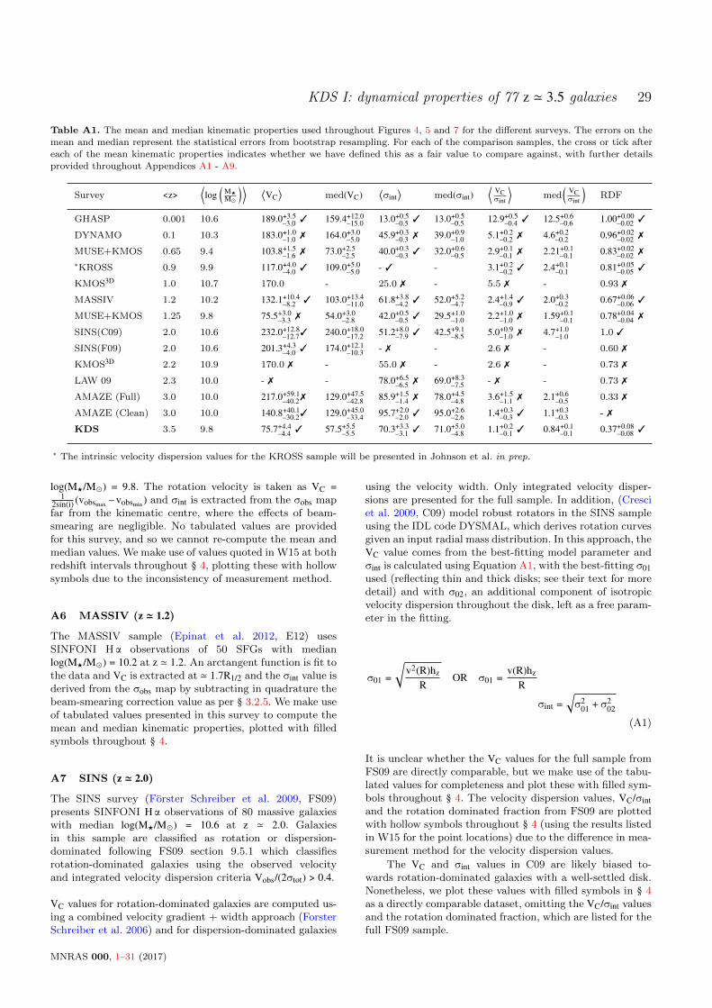
KDS I: dynamical properties of 77 z ' 3.5 galaxies 29

Table A1. The mean and median kinematic properties used throughout Figures 4, 5 and 7 for the different surveys. The errors on themean and median represent the statistical errors from bootstrap resampling. For each of the comparison samples, the cross or tick after

each of the mean kinematic properties indicates whether we have defined this as a fair value to compare against, with further details

provided throughout Appendices A1 - A9.

Survey <z>⟨log

(M?M�

)⟩ ⟨VC

⟩med(VC)

⟨σint

⟩med(σint)

⟨VCσint

⟩med

(VCσint

)RDF

GHASP 0.001 10.6 189.0+3.5–3.0 3 159.4+12.0–15.0 13.0+0.5–0.5 3 13.0+0.5–0.5 12.9+0.5–0.4 3 12.5+0.6–0.6 1.00+0.00–0.02 3

DYNAMO 0.1 10.3 183.0+1.0–1.0 7 164.0+3.0–5.0 45.9+0.3–0.3 7 39.0+0.9–1.0 5.1+0.2–0.2 7 4.6+0.2–0.2 0.96+0.02–0.02 7

MUSE+KMOS 0.65 9.4 103.8+1.5–1.6 7 73.0+2.5–2.5 40.0+0.3–0.3 3 32.0+0.6–0.5 2.9+0.1–0.1 7 2.21+0.1–0.1 0.83+0.02–0.02 7

∗KROSS 0.9 9.9 117.0+4.0–4.0 3 109.0+5.0–5.0 - 3 - 3.1+0.2–0.2 3 2.4+0.1–0.1 0.81+0.05–0.05 3

KMOS3D 1.0 10.7 170.0 - 25.0 7 - 5.5 7 - 0.93 7

MASSIV 1.2 10.2 132.1+10.4–8.2 3 103.0+13.4–11.0 61.8+3.8–4.2 3 52.0+5.2–4.7 2.4+1.4–0.9 3 2.0+0.3–0.2 0.67+0.06–0.06 3

MUSE+KMOS 1.25 9.8 75.5+3.0–3.3 7 54.0+3.0–2.8 42.0+0.5–0.5 3 29.5+1.0–1.0 2.2+1.0–1.0 7 1.59+0.1–0.1 0.78+0.04–0.04 7

SINS(C09) 2.0 10.6 232.0+12.8–12.73 240.0+18.0–17.2 51.2+8.0–7.9 3 42.5+9.1–8.5 5.0+0.9–1.0 7 4.7+1.0–1.0 1.0 3

SINS(F09) 2.0 10.6 201.3+4.3–4.0 3 174.0+12.1–10.3 - 7 - 2.6 7 - 0.60 7

KMOS3D 2.2 10.9 170.0 7 - 55.0 7 - 2.6 7 - 0.73 7

LAW 09 2.3 10.0 - 7 - 78.0+6.5–6.5 7 69.0+8.3–7.5 - 7 - 0.73 7

AMAZE (Full) 3.0 10.0 217.0+59.1–40.27 129.0+47.5–42.8 85.9+1.5–1.4 7 78.0+4.5–4.8 3.6+1.5–1.1 7 2.1+0.6–0.5 0.33 7

AMAZE (Clean) 3.0 10.0 140.8+40.1–30.23 129.0+45.0–33.4 95.7+2.0–2.0 3 95.0+2.6–2.6 1.4+0.3–0.3 3 1.1+0.3–0.3 - 7

KDS 3.5 9.8 75.7+4.4–4.4 3 57.5+5.5–5.5 70.3+3.3–3.1 3 71.0+5.0–4.8 1.1+0.2–0.1 3 0.84+0.1–0.1 0.37+0.08–0.08 3

∗ The intrinsic velocity dispersion values for the KROSS sample will be presented in Johnson et al. in prep.

log(M?/M�) = 9.8. The rotation velocity is taken as VC =1

2sin(i) (vobsmax – vobsmin ) and σint is extracted from the σobs mapfar from the kinematic centre, where the effects of beam-smearing are negligible. No tabulated values are providedfor this survey, and so we cannot re-compute the mean andmedian values. We make use of values quoted in W15 at bothredshift intervals throughout § 4, plotting these with hollowsymbols due to the inconsistency of measurement method.

A6 MASSIV (z ' 1.2)

The MASSIV sample (Epinat et al. 2012, E12) usesSINFONI H α observations of 50 SFGs with medianlog(M?/M�) = 10.2 at z ' 1.2. An arctangent function is fit tothe data and VC is extracted at ' 1.7R1/2 and the σint value isderived from the σobs map by subtracting in quadrature thebeam-smearing correction value as per § 3.2.5. We make useof tabulated values presented in this survey to compute themean and median kinematic properties, plotted with filledsymbols throughout § 4.

A7 SINS (z ' 2.0)

The SINS survey (Forster Schreiber et al. 2009, FS09)presents SINFONI H α observations of 80 massive galaxieswith median log(M?/M�) = 10.6 at z ' 2.0. Galaxiesin this sample are classified as rotation or dispersion-dominated following FS09 section 9.5.1 which classifiesrotation-dominated galaxies using the observed velocityand integrated velocity dispersion criteria Vobs/(2σtot) > 0.4.

VC values for rotation-dominated galaxies are computed us-ing a combined velocity gradient + width approach (ForsterSchreiber et al. 2006) and for dispersion-dominated galaxies

using the velocity width. Only integrated velocity disper-sions are presented for the full sample. In addition, (Cresciet al. 2009, C09) model robust rotators in the SINS sampleusing the IDL code DYSMAL, which derives rotation curvesgiven an input radial mass distribution. In this approach, theVC value comes from the best-fitting model parameter andσint is calculated using Equation A1, with the best-fitting σ01used (reflecting thin and thick disks; see their text for moredetail) and with σ02, an additional component of isotropicvelocity dispersion throughout the disk, left as a free param-eter in the fitting.

σ01 =

√v2(R)hz

ROR σ01 =

v(R)hzR

σint =√σ201 + σ

202

(A1)

It is unclear whether the VC values for the full sample fromFS09 are directly comparable, but we make use of the tabu-lated values for completeness and plot these with filled sym-bols throughout § 4. The velocity dispersion values, VC/σintand the rotation dominated fraction from FS09 are plottedwith hollow symbols throughout § 4 (using the results listedin W15 for the point locations) due to the difference in mea-surement method for the velocity dispersion values.

The VC and σint values in C09 are likely biased to-wards rotation-dominated galaxies with a well-settled disk.Nonetheless, we plot these values with filled symbols in § 4as a directly comparable dataset, omitting the VC/σint valuesand the rotation dominated fraction, which are listed for thefull FS09 sample.

MNRAS 000, 1–31 (2017)

30 O.J. Turner et al.

A8 LAW 09 (z ' 2.3)

In (Law et al. 2009, L09) OSIRIS [O III]λ5007 and H αobservations are collected for 13 galaxies with medianlog(M?/M�) = 10.0 at z ' 2.3. The ‘velocity shear’ is com-puted as vshear = 1

2 (vmax –vmin) without inclination correctionand σint is the flux-weighted mean of σobs. We note that theσmean values and errors tabulated in the Law et al. (2009)paper are the flux-weighted mean and standard deviationof the measurements in individual spaxels in each galaxy,not corrected for beam-smearing in any way. These mea-surements are expected to be larger than the σint measure-ments at similar redshift which have been beam-smearingcorrected, or extracted at the galaxy outskirts where the ef-fects of beam-smearing are much smaller. We use tabulateddata σint data in L09 to compare this distribution with otherresults, but plot with a hollow symbol due to the lack of abeam-smearing correction.

A9 AMAZE (z ' 3.0)

The AMAZE sample (Gnerucci et al. 2011, G11) presentsSINFONI [O III]λ5007 measurements for 33 galaxies withmedian log(M?/M�) = 9.9 at z ' 3, closest in redshiftto the KDS galaxies. In this study, rotation curves andintrinsic velocity dispersions are derived from a modelledexponential mass distribution, with the extracted VC valuetaken as the large radius limit of the rotation curve andthe σint as the maximum of the difference in quadraturebetween the σobs map and the σmodel map (which also takesinto account instrumental resolution and beam-smearing;see their Equation 8). A caveat when comparing with theG11 values is that dynamical properties are computed for11 rotation-dominated galaxies in their sample, with theremaining 22 galaxies not analysed.

Also, for 5 galaxies in G11, VC is not well constrained andno errorbar is given; for these objects we take the fractionalerror on VC equal to 1 when computing the sample aver-ages. The σint errors for individual galaxies are generallyvery small, and for 3 galaxies the σint value is consistentwith 0 km s–1. For the mean value computation for the fullsample we set these equal to the SINFONI resolution limitof 30 km s–1. A total of 6/11 galaxies either have no errors onVC or have σint values consistent with 0 km s–1, which we re-fer to as the AMAZE ‘Unconstrained’ sample and representthese with hollow symbols throughout the plots in § 4.This Unconstrained sample also contains the galaxys sa22a-M38, common between the KDS and G11, classifiedhere as a merger due to double HST components and twinpeaks in the object spectrum, but classified in G11 as arotating galaxy with VC = 346km s–1 (although the authorsdiscuss the possibility that the galaxy could be eithera close pair or two clumps embedded within a rotatingdisk). We use tabulated values from the full analysedsample of 11 galaxies, plotting these with hollow symbolsthroughout § 4 as a consequence of the caveats listed above.The 5/11 galaxies which are not in the Unconstrainedsample are referred to as the AMAZE ‘Clean sample’ andare directly comparable to the KDS. These are plottedwith filled symbols throughout § 4. We plot the quotedrotation-dominated fraction of 33% as a hollow symbol,

Figure B1. The distribution of the isolated field sample in the

σint vs. VC plane is plotted with the red symbols. The AMAZE

Clean (z ' 3) sample galaxies (see appendix A9) are plotted withgrey symbols and the AMAZE Unconstrained sample with hol-

low symbols. There is no strong correlation between the two

parameters in either of these surveys and we note that theKDS and AMAZE Clean galaxies are generally in agreement.

The VC/σint = 1 line divides the galaxies classified as rotation-

dominated and dispersion-dominated. The galaxy s sa22a-M38,

classified here as a merger but classified in Gnerucci et al. (2011)

as a rotating galaxy with VC = 346km s–1 is marked on the plot.

noting that this could be higher if any of the 22/33 galaxiesnot analysed are rotation-dominated.

This comparison sample summary shows that there aremany different approaches for computing the same intrinsickinematic parameters, dictated by data quality and modelpreference, however, despite this diversity, over the pastdecade the studies appear to be converging on ‘modellingout’ the effects of beam-smearing using similar approaches(e.g. as described in Davies et al. 2011, where removingthe effects of beam-smearing with spectrally and spatiallyconvolved models is also the least biased approach). Thistrend towards consistency is encouraging, and, as describedin § 3.2.2, we have also shaped our approach towards ex-tracting intrinsic kinematic parameters after correcting forbeam-smearing effects quantified in the modelling. We stressthat, keeping in mind sample selection, mass ranges andkinematic parameter extraction methods are crucial whencomparing results between different surveys.

APPENDIX B: INTRINSIC PARAMETERDISTRIBUTIONS

In Figure B1 we plot the distribution of the isolatedfield sample in the σint vs. log(VC) plane. The VC = σintline roughly bisects the KDS sample, and separates the

MNRAS 000, 1–31 (2017)

KDS I: dynamical properties of 77 z ' 3.5 galaxies 31

dispersion-dominated and rotation-dominated galaxies bydefinition. The isolated field sample galaxies are clusteredaround a relatively tight region in both VC and σint and thereis good agreement between the KDS and AMAZE Clean(z ' 3) samples. The galaxies in the AMAZE Unconstrainedsample generally have much larger VC values despite occupy-ing a similar stellar mass range to our isolated field sample,with this being a consequence of large model extrapolationsbeyond the observed data. We follow the bootstrapping pro-cedure described in Appendix A to compute error weightedaverages and statistical errors.

APPENDIX C: KINEMATIC PARAMETERSERROR ESTIMATES

C1 3D modelling kinematic parameter errorestimates

As mentioned in § 3.2.2, the MCMC sampling provides dis-tributions for each of the model parameters, from which wecan extract the 84th and 16th percentile values as the +/-1-σ errors. During the following procedure, PAkin is fixedto the maximum-likelihood value for all model evaluations.We proceed to reconstruct the beam-smeared and intrinsicdynamical models for each of the isolated field galaxies us-ing the 16th and 84th percentile parameters, with the lowervelocity 16th percentile model constructed using the upperlimit on the inclination, and the 84th percentile model us-ing the lower limit. To clearly distinguish the 1-σ error re-gions for both the beam-smeared and intrinsic models, theregion between the 16th and 84th percentile evaluations isshaded blue and red respectively in the velocity extactionpanels throughout Figures D1 and D2. The +/- 1-σ errorvalues for both VC are then calculated using the equationsbelow, which also take into account the measurement errors,with σvobs equal to the average observational uncertainty ex-tracted along PAkin. The subscripts ‘16th’ and ‘84th’ denotethe parameters used to construct the model from which thevelocity has been extracted.

δVC+ =√(VC–84 – VC)2 +

(δVobs

)2(C1)

δVC– =√(VC – VC–16)2 +

(δVobs

)2(C2)

The upper and lower errors on the σint are calculated using asimilar approach. To encorporate the uncertainty introducedin the modelling by assuming a fixed value of σint = 50km s–1,we make two further model evaluations using both the 16thand 84th percentile parameters with σint = 40km s–1 andσint = 80km s–1, with these representing reasonable minimumand maximum mean instrinsic sigma values (chosen by con-sidering the range in σint at similar redshift, see e.g. Fig-ure 5). When assuming the broader σint = 80km s–1 value ineach spaxel the beam-smearing correction decreases, as theimpact of convolution with spectral lines in adjacent spax-els with shifted velocity centres is less severe. Conversely,assuming σint = 40km s–1 increases the beam-smearing. Wecalculate the minimum and maxmimum intrinsic velocity

dispersion, σint–84–40 and σint–16–80, using equations C3 andC4 respectively:

σint–84–40 =√(σobs – σbs–84–40)2 – σ2sky (C3)

σint–16–80 =√(σobs – σbs–16–80)2 – σ2sky (C4)

where σbs–84–40 = σmodel–84–40 –40 and σbs–16–80 = σmodel16–80 –80 are the beam-smeared maps. The lower and upper errorson σint are then given by the following:

δσint+ =√(σint – σint–84–40)2 +

(σσobs

)2(C5)

δσint– =√(σint–16–80 – σint)2 +

(σσobs

)2(C6)

with σσobs equal to the average of the velocity dispersionmeasurement errors. Once these quantities have been mea-sured, the upper and lower errors on the ratio VC/σint canbe computed using equations C7 and C8.

δVCσint

+ =VCσint

√(δVC+VC

)2+

(δσint+σint

)2(C7)

δVCσint

– =VCσint

√(δVC–VC

)2+

(δσint + –σint

)2(C8)

APPENDIX D: KINEMATICS PLOTS

In Figures D1, D2 and D3 we plot the kinematic grids for theKDS galaxies classified as rotation-dominated, dispersion-dominated and merger candidates respectively. The figurecaptions provide more information on each of the panels ofthese grids.

This paper has been typeset from a TEX/LATEX file prepared bythe author.

MNRAS 000, 1–31 (2017)

32 O.J. Turner et al.

Figure D1. We plot the kinematic grids for the 13/32 isolated field sample galaxies classified as rotation-dominated. For each galaxy

we plot the HST image, GALFIT model and GALFIT residuals, along with the observed [O III]λ5007 intensity map, dispersion map andvelocity map extracted from the datacubes with gaussian-fits to the individual spaxels as described in § 3.2.1. The solid black line anddashed orange line plotted in various panels show PAkin and PAmorph respectively. On the bottom row we plot the beam-smeared model

velocity and data-model velocity residuals with colour bar limits tuned to the velocity model. Also on the bottom row, we plot extractions

along PAkin for both the velocity and velocity dispersion. The grey points with errorbars on the velocity extraction plot are from theobserved velocity map, the blue line and blue shaded regions represent the beam-smeared model fit to the data and errors respectively,

whereas the red line and shaded regions are the intrinsic model from which VC is extracted. The purple symbols represent the extractionalong PAkin from the residual map, and the two vertical dashed lines denote the intrinsic (inner) and convolved (outer) 2R1/2 values,

with VC extracted at the intrinsic value and VBS extracted at the convolved value of the intrinsic and observed profiles respectively. The

intrinsic models flatten at small radii, and so small changes in R1/2 have negligible impact on the final, extracted VC values. The bluepoints on the velocity dispersion extraction plot show the values extracted from the observed dispersion map and the red are from the

beam-smearing corrected map as per Equation 6, and the vertical dashed lines have the same meaning as for the velocity extraction

plot. Also plotted with the blue and red dot-dash horizontal lines are the median values of the observed and intrinsic (i.e. σint) dispersionmaps respectively.

MNRAS 000, 1–31 (2017)

KDS I: dynamical properties of 77 z ' 3.5 galaxies 33

Figure D1. Continued.MNRAS 000, 1–31 (2017)

34 O.J. Turner et al.

Figure D1. Continued. MNRAS 000, 1–31 (2017)

KDS I: dynamical properties of 77 z ' 3.5 galaxies 35

Figure D1. Continued.

MNRAS 000, 1–31 (2017)

36 O.J. Turner et al.

Figure D2. The same as in figure D1 but for the dispersion-dominated galaxies. MNRAS 000, 1–31 (2017)

KDS I: dynamical properties of 77 z ' 3.5 galaxies 37

Figure D2. Continued.MNRAS 000, 1–31 (2017)

38 O.J. Turner et al.

Figure D2. Continued. MNRAS 000, 1–31 (2017)

KDS I: dynamical properties of 77 z ' 3.5 galaxies 39

Figure D2. Continued.MNRAS 000, 1–31 (2017)

40 O.J. Turner et al.

Figure D2. Continued.

MNRAS 000, 1–31 (2017)

KDS I: dynamical properties of 77 z ' 3.5 galaxies 41

Figure D3. The same as for figure D1 but for the merger candidates. In this case we plot only fits to the data in the velocity extraction

plot with the blue line, rather than attempting the full beam-smearing analysis. Several of the galaxies here mimic rotation from a purelykinematic perspective, but have two or more HST components and an accompanying double peak in the object spectrum at the objectcentre, leading to large velocity dispersions when single gaussian-fits are attempted.

MNRAS 000, 1–31 (2017)

42 O.J. Turner et al.

Figure D3. Continued. MNRAS 000, 1–31 (2017)

KDS I: dynamical properties of 77 z ' 3.5 galaxies 43

Figure D3. Continued.MNRAS 000, 1–31 (2017)

44 O.J. Turner et al.

Figure D3. Continued.

MNRAS 000, 1–31 (2017)