i

MIXED LIQUID BAG PACKING SYSTEM USING PLC

A PROJECT REPORT

Submitted by,

YAGNIK PATEL (090420117013)

MOHAMMED PAGHDIWALA (090420117019)

PARTH BHIMANI (090420117021)

SAGAR THAKKAR (100420117003)

In fulfilment for the award of the degree

Of

BACHELOR OF ENGINEERING

In

INSTRUMENTATION & CONTROL

SARVAJANIK COLLLAGE OF ENGINEERING AND TECHNOLOGY

SURAT

Gujarat Technological University, Ahmedabad

December, 2011

SARVAJANIK COLLEGE OF ENGINEERING AND TECHNOLOGY

ii

SURAT

DEPARTMENT OF INSTRUMENTATION & CONTROL

CERTIFICATE

Date:

This is to certify that the dissertation entitled “MIXED LIQUID BAG PACKING

SYSTEM USING PLC” has been carried out by Yagnik Patel, Parth Bhimani, Sagar

Thakkar, Mohammed Paghdiwala under my guidance in fulfilment of the degree of

Bachelor of Engineering in INSTRUMENTATION & CONTROL(7th Semester) of

Gujarat Technological University, Ahmedabad during the academic year 2012-13.

Guide: Prof. Tejal Dave

Prof. Utpal Pandya

Head of the Department

iii

Abstract

The report of Project entitled “Mixed Liquid Bag Packing System” has mainly description of the

Mechanical Assembly section, Electronics Hardware and Software Section.

In the mechanical assembly section all the mechanical hardware like motor, gear box, chain &

cams and support are described in details. The specification of all the parts are given. The

Principle and working of all the mechanical parts are described.

In the electronics hardware section the description and specification of different IC’s like voltage

regulator (KA7812), relays (MY2N), LED, solid state relay voltage limiter, pt100 with digital

display and solenoid valve.

In the software section the programming language in ladder diagram using the software WPLSoft

2.33.

PLC has evolved as an important controller in industries these days because of its simplicity and

robustness. It is used for controlling many mechanical movements of the heavy machines or to

control the voltage and frequency of the power supplies.

In this project, study of the PLC has been done in great detail and also several industrial

applications have been studied and realized through ladder diagrams. The applications on which

we have stressed are the liquid mixing system and continuous bag packing system. Both parts

are PLC based and automated. It is batch process. This process has wide application in

processing industries.

iv

Acknowledgement

We would like to thank all the people who helped in the completing this Project and the report

possible:

The Almighty Lord

Nothing is possible without the blessing of the Almighty and we would like to thank him with

all my heart and soul for giving us mental and physical strength to prepare this project and report.

Our Respected guide

First of all, we would like to express your gratitude and sincere thanks to my respected

Faculty assistant Prof. Tejal Dave for his professional guidance, advice, motivation, endurance

and encouragements d u r i ng his supervision pe r iod . The present work would have never

been possible without his vital supports and valuable assistance.

Then w e would like to thank all yo u r friends who have knowingly or unknowingly tips and

views were useful indeed and then thanks to the other faculty members and staff of the

Department of Instrumentation and Control Engineering, SCET, Surat for their extreme help

throughout my course of study at this institute.

v

List of figures:-

Figure 1.1 Automation: typical installation...................................................................... . .4

Figure 1.2 Automation: Advanced technology...............................................................5

Figure 2.1 PLC conceptual application diagram …….............................................................6

Figure 2.2 Basic parts of PLC ……………………………………………………………………………...…7

Figure 2.3 Hardwired logic circuit and its PLC ladder diagram representation ……………..13

Figure 2.4 Hardwired logic circuit and its Boolean expression ……………………………....13

Figure 3.1 Worked Flow Diagram…………………………………………………………….15

Figure 3.2 Solenoid valve………………………………………………………………………16

Figure 3.3 DC Motor………………..………………………………………………………….17

Figure3.4RelayMY2N……………..……………………………………………………………19

Figure 4.1 Block diagram…………………………………………………………………..21

Figure 4.2 Complete Flow diagram…………………………………………………………21

1

TABLE OF CONTENTS

Acknowledgement

Abstract

List of Figures

Table of Contents

iii

iv

v

vi

Chapter : 1 Industrial Automation

1.1 Introduction

2

1.2 History of Automation 3

1.3 Industrial Automation Components 4

1.4 Automation : Advanced Technology 5

Chapter : 2 Programmable Logic Controller (PLC)

2.1 What is PLC? 6

2.2 Need of PLC 11

2.3 Delta DVP28SV 12

2.4 Programming languages 14

2.5 Advantages of PLC 15

Chapter: 3 Liquid Mixing System

3.1 Introduction

15

3.2 List of Components 16

3.2.1 Level Sensor 16 3.2.2 Solenoid Valve

16

3.2.3 Stirrer 17

3.2.4 DC Motor 17

3.2.5 2/2way continuous diaphragm type valve 19

3.2.6 Relay MY2N 19

3.2.7 IC KA7812 20

Chapter: 4 Works until now

Chapter: 5 Future planning

4.1 Bag packing system 26

References 27

.

2

Chapter 1

Industrial Automation

1.1 Introduction

Automation is the use of machines, control systems and information technologies to optimize

productivity in the production of goods and delivery of services. The correct incentive for applying

automation is to increase productivity, and/or quality beyond that possible with current human labor

levels so as to realize economies of scale, and/or realize predictable quality levels.

The incorrect application of automation, which occurs most often, is an effort to eliminate or replace

human labor. Simply put, whereas correct application of automation can net as much as 3 to 4 times

original output with no increase in current human labor costs, incorrect application of automation can

only save a fraction of current labor level costs. In the scope of industrialization, automation is a step

beyond mechanization. Whereas mechanization provides human operators with machinery to assist

them with the muscular requirements of work, automation greatly decreases the need for human

sensory and mental requirements while increasing load capacity, speed, and repeatability.

Automation plays an increasingly important role in the world economy and in daily experience.

Automation has had a notable impact in a wide range of industries beyond manufacturing (where it

began). Once-ubiquitous telephone operators have been replaced largely by automated telephone

switchboards and answering machines. Medical processes such as primary screening in

electrocardiography or radiography and laboratory analysis of human genes, sera, cells, and tissues are

carried out at much greater speed and accuracy by automated systems.

Automated teller machines have reduced the need for bank visits to obtain cash and carry out

transactions. In general, automation has been responsible for the shift in the world economy from

industrial jobs to service jobs in the 20th and 21st centuries. The term automation, inspired by the

earlier word automatic (coming from automaton), was not widely used before 1947, when General

Motors established the automation department. At that time automation technologies were electrical,

mechanical, hydraulic and pneumatic. Between 1957 and 1964 factory output nearly doubled while the

number of blue collar workers started to decline.

1.2 History of Automation

1) Programmable Logic Controller

2) Electronic Control using Logic Gates

3) Hard wired logic Control

4) Pneumatic Control

5) Manual Control

3

1) Programmable Logic Controller :

In 1970s with the coming of microprocessors and associated peripheral chips, the whole process of

control and automation underwent a radical change. Instead of achieving the desired control or

automation through physical wiring of control devices, in PLC it is achieved through a program or

say software. The programmable controllers have in recent years experienced an unprecedented

growth as universal element in Industrial Automation. It can be effectively used in applications

ranging from simple control like replacing small number of relays to complex automation problems.

2) Electronic Control using Logic Gates :

In 1960s with the advent of electronics, the logic gates started replacing the relays and auxiliary

contactors in the control circuits. The hardware timers & counters were replaced by electronic timer.

Advantages

Reduced space requirements

Energy saving

Less maintenance & greater reliability Drawbacks

Changes in control logic not possible

More project time reduced space

Ease of maintenance

Economical

Greater life & reliability

3) Hard wired logic Control

The contractor and relays together with hardware timers and counters were used in achieving the

desired level of automation.

Drawbacks

Bulky panels

Complex wiring

Longer project time

Difficult maintenance and troubleshooting

4) Pneumatic Control

Industrial automation, with its machine and process control, had its origin in the 1920s with the

advent of "Pneumatic Controllers".

Actions were controlled by a simple manipulation of pneumatic valves, which in turn were

controlled by relays and switches.

Drawbacks

Bulky and Complex System

Involves lot of rework to implement control logic

Longer project time

4

5) Manual Control

All the actions related to process control are taken by the Operators.

Drawbacks

Likely human errors and consequently its effect on quality of final product

The production, safety, energy consumption and usage of raw material are all subject to the

correctness and accuracy of human action.

1.3 Industrial Automation Components

Field Instruments

Control Hardware

Control Software

Fig. 1.1 Automation: Typical installation

1.4 Automation: Advanced Technology

5

Fig. 1.2 Automation: Advanced Technology

6

Chapter 2 Programmable Logic Controller (PLC)

2.1 What is PLC?

Introduction

A programmable logic controller, commonly known as PLC, is a solid state, digital, industrial

computer using integrated circuits instead of electromechanical devices to implement control functions.

It was invented in order to replace the sequential circuits which were mainly used for machine control.

They are capable of storing instructions, such as sequencing, timing, counting, arithmetic, data

manipulation and communication, to control machines and processes.

According to NEMA (National Electrical Manufacture’s Association, USA), the definition of PLC has

been given as

“Digital electronic devices that uses a programmable memory to store instructions and to

implement specific functions such as logic , sequencing, timing, counting, and arithmetic to control

machines and processes.”

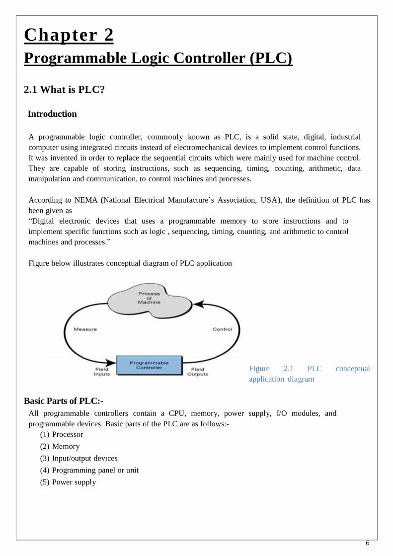
Figure below illustrates conceptual diagram of PLC application

Figure 2.1 PLC conceptual

application diagram

Basic Parts of PLC:-

All programmable controllers contain a CPU, memory, power supply, I/O modules, and

programmable devices. Basic parts of the PLC are as follows:-

(1) Processor

(2) Memory

(3) Input/output devices

(4) Programming panel or unit

(5) Power supply

7

Processor’s Module:-

Processor module is the brain of the PLC. Intelligence of the PLC is derived from microprocessor

being used which has the tremendous computing and controlling capability.

Central processing unit (CPU) performs the following tasks:-

Scanning

Execution of program

Peripheral and external device communication

Self- diagnostic

Power of PLCs depends on the type of microprocessors being used. Small size PLCs use 8-bit

microprocessors where as higher order controllers use bit-slice microprocessor in order to achieve

faster instruction execute

Modern day PLCs vary widely in their capabilities to control real world devices, like some processors

are able to handle the I/O devices as few as six and some are able to handle 40000 or more. The no. of

input/output control of PLCs depends on the, hardware, software, overall capacity and memory

capability of the PLCs.

The CPU upon receiving instruction from the memory together with feedback on the status of the I/O

devices generates commands for the output devices. These commands control the devices on a machine

or a process. Devices such as solenoid valves, indicator lamps, relay coils and motor starters and typical

loads to be controlled.

The machine or process input elements transmit signal to input modules which in turn, generates logic

signal to the CPU.CPU monitors the input like selector switches, push buttons etc.

8

Operating system is the main workhouse of the system and hence performs the following tasks:-

1. Executions of application program

2. Management of memory

3. Communication between programmable controller and other units

4. I/O handling of interfaces

5. Resource sharing

6. Diagnostics

Note: - operating system stored in ROM (non –volatile) memory, whereas application program are

stored in RWM (read-write memory).

Input modules:-

There are many types of input modules to choose from. The type of input module selection depends

upon the process, some example of input modules are limit :-switches, proximity switches and push

buttons etc. nature of input classification can be done in three ways, namely:-

low/high frequency

analog/digital (two-bit, multi-bit)

maintained or momentary

5V/24V/110V/220V switched

Some most industrial power systems are inherently noisy: -

Electrical isolation is provided between the input and the processor. Electromagnetic interference

(EMI) and radio frequency interference (RFI) can cause severe problems in most solid state

control systems. The component used often to provide electrical isolation within I/O cards is

called an optical isolator or opto-coupler. Typically, there are 8 to 32 input points on any one

input modules. Each input point is assigned a unique address by the processor.

Output modules:-

Output modules can be used for devices such as solenoids, relays, contractors, pilot lamps and led

readouts. Output cards usually have 6 to 32 output points on a single module. Output cards, like input

cards, have electrically isolation between the load being connected and the PLC. Analog output cards

are a special type of output modules that use digital to analog conversion. The analog output module

can take a value stored in a 12 bit file and convert it to an analog signal. Normally, this signal is 0-10

volts dc or 4-20ma. This analog signal is often used in equipment, such as motor-operated valves and

pneumatic position control device. Each output point is identified with a unique address.

Addressing scheme:-

Each I/O device has to be identified with a unique address for exchange of data. Different manufacturer

apply different method to identify I/O devices. One of the addressing schemes may be “X1 X2 X3 X4

X5” where

X1 = input or output designation fixed by hardware (I/p = 1, O/p = 0)

X2 = I/O rack number in PLC (user designation)

X3 = modules slot number in I/O rack (fixed by hardware) X4, X5 =

9

terminal number (fixed by hardware)

For example,” 1 2 3 13” implies that input is at rack 2, module slot no.3 and terminal address

no.13.

Programming unit:-

It is an external, electronic handheld device which can be connected to the processors of the PLC when

programming changes are required. Once a program has been coded and is considered finished, It can be

burned in to ROM. The contents of ROM cannot be altered, as it is not affected by power failure. Now a

days EPROM/EEPROM are provided in which program can be debugged at any stage. Once the

program is debugged, programming unit is disconnected; and the PLC can operate process according to

the ladder diagram or the statement list.

Communications in PLC:-

There are several methods how a PLC can communicate with the programmer, or even with

another PLC. PLCs usually built in communication ports for at least RS232, and optionally for RS

485, and Ethernet. Modbus is the lowest common denominator communication protocol. Others are

various fieldbuses such as profibus, interbus-s, foundation field bus, etc.

PLCs are becoming more and more intelligent .in recent years, PLCs have been integrated in to

industrial networks, and all the PLCs in an industrial environment have been plugged in to a network.

The PLCs are then supervised by a control center. There exist many types of networks, SCADA

(supervisory control and data acquisition)

Operation in PLC:-

During program execution, the processor reads all the inputs, and according to control application

program, energizes and de-energizes the outputs. Once all the logic has been solved, the processors will

update all the outputs. The process of reading the inputs, executing the control application program, and

updating the output is known as scan. During the scan operation, the processor also performs

housekeeping tasks.

The inputs to the PLCs are sampled by processor and the contents are stored in memory. Control

program is executed, the input value stored in memory are used in control logic calculations to

determine the value of output. The outputs are then updated.

The cycle consisting of reading of inputs, executing the control program, and actuating the output is

known as “scan” and the time to finish this task is known as “scan time”. The speed at which PLC scan

depends upon the clock speed of CPU. The time to scan depends upon following parameter:-

Scan rate

Length of the program

Types of functions used in the program

Faster scan time implies the inputs and outputs are updated frequently. Due to advance techniques of

ASIC (application specific integrated circuit) within the microcomputer for specific functions, scan time

of different PLCs have reduced greatly.

10

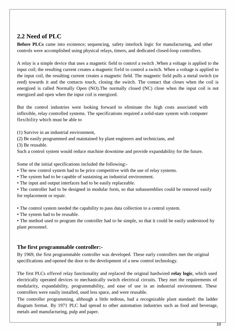
2.2 Need of PLC Before PLCs came into existence; sequencing, safety interlock logic for manufacturing, and other

controls were accomplished using physical relays, timers, and dedicated closed-loop controllers.

A relay is a simple device that uses a magnetic field to control a switch .When a voltage is applied to the

input coil; the resulting current creates a magnetic field to control a switch. When a voltage is applied to

the input coil, the resulting current creates a magnetic field. The magnetic field pulls a metal switch (or

reed) towards it and the contacts touch, closing the switch. The contact that closes when the coil is

energized is called Normally Open (NO).The normally closed (NC) close when the input coil is not

energized and open when the input coil is energized.

But the control industries were looking forward to eliminate the high costs associated with

inflexible, relay controlled systems. The specifications required a solid-state system with computer

flexibility which must be able to

(1) Survive in an industrial environment,

(2) Be easily programmed and maintained by plant engineers and technicians, and

(3) Be reusable.

Such a control system would reduce machine downtime and provide expandability for the future.

Some of the initial specifications included the following:-

• The new control system had to be price competitive with the use of relay systems.

• The system had to be capable of sustaining an industrial environment.

• The input and output interfaces had to be easily replaceable.

• The controller had to be designed in modular form, so that subassemblies could be removed easily

for replacement or repair.

• The control system needed the capability to pass data collection to a central system.

• The system had to be reusable.

• The method used to program the controller had to be simple, so that it could be easily understood by

plant personnel.

The first programmable controller:-

By 1969, the first programmable controller was developed. These early controllers met the original

specifications and opened the door to the development of a new control technology.

The first PLCs offered relay functionality and replaced the original hardwired relay logic, which used

electrically operated devices to mechanically switch electrical circuits. They met the requirements of

modularity, expandability, programmability, and ease of use in an industrial environment. These

controllers were easily installed, used less space, and were reusable.

The controller programming, although a little tedious, had a recognizable plant standard: the ladder

diagram format. By 1971 PLC had spread to other automation industries such as food and beverage,

metals and manufacturing, pulp and paper.

11

The conceptual design of PLC:-

The first programmable controllers were more or less just relay replacers. Their primary function was to

perform the sequential operations that were previously implemented with relays. These operations

included ON/OFF control of machines and processes that required repetitive operations, such as transfer

lines and grinding and boring machines. However, these programmable controllers were a vast

improvement over relays. They were easily installed, used considerably less space and energy, had

diagnostic indicators that aided troubleshooting, and unlike relays, were reusable if a project was

scrapped.

Although PLC functions, such as speed of operation, types of interfaces, and data-processing

capabilities, have improved throughout the years, their specifications still hold to the designers’

original intentions—they are simple to use and maintain.

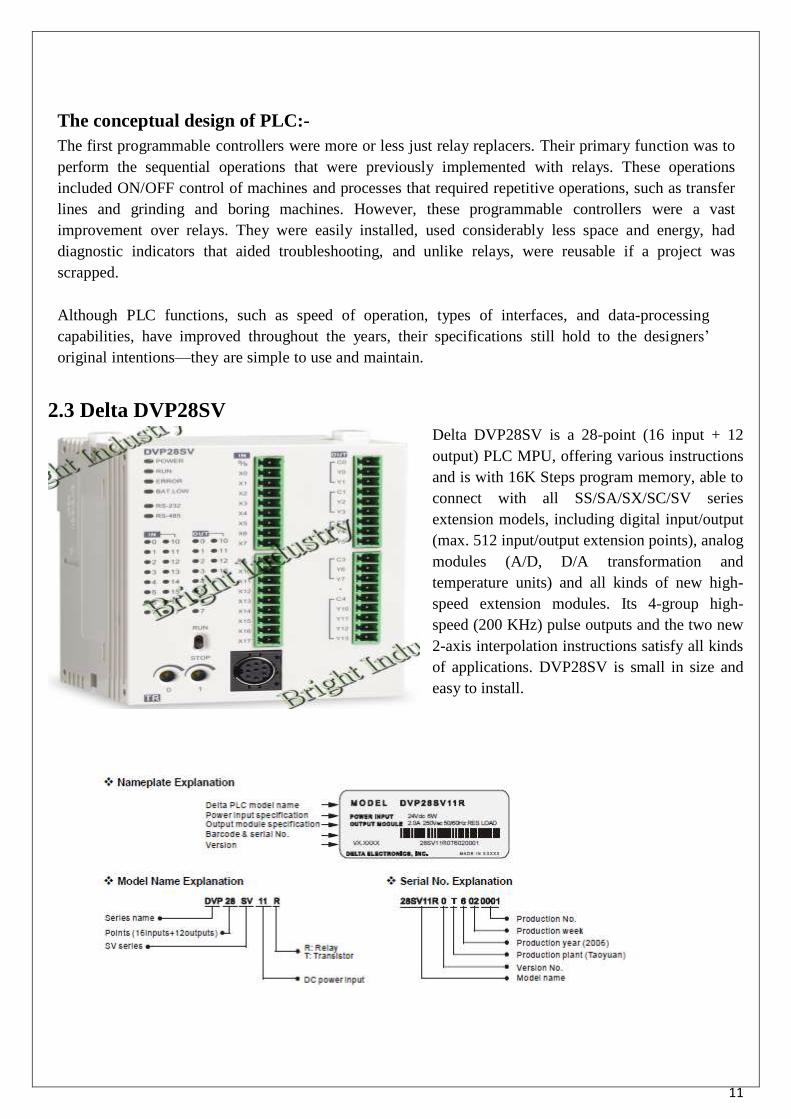
2.3 Delta DVP28SV Delta DVP28SV is a 28-point (16 input + 12

output) PLC MPU, offering various instructions

and is with 16K Steps program memory, able to

connect with all SS/SA/SX/SC/SV series

extension models, including digital input/output

(max. 512 input/output extension points), analog

modules (A/D, D/A transformation and

temperature units) and all kinds of new high-

speed extension modules. Its 4-group high-

speed (200 KHz) pulse outputs and the two new

2-axis interpolation instructions satisfy all kinds

of applications. DVP28SV is small in size and

easy to install.

12

Product Profile and Outline

1) 1 POWER/RUN/BAT.LOW/ERROR indicator

2) COM1 (RS-232) receiving communication (Rx) indicator

3) COM2 (RS-485) sending communication (Tx) indicator

4) Input/output indicator

5) RUN/STOP switch

6) VR0: M1178 enabled/D1178 corresponding value

7) VR1: M1179enabled/D1179 corresponding value

8) Input/output terminal

9) COM1 (RS-232) program I/O communication port

10) DIN rail clip

11) Extension module positioning hole

12) Extension module connection port

13) DIN rail (35mm)

14) Extension module fastening clip

15) COM2 (RS-485) communication port (Master/Slave)

16) Power input port

17) 3 P removable terminal (standard component)

18) Power input connection cable (standard component)

19) New high-speed extension module connection port

20) Nameplate

21) Direct fastening hole

13

Electrical specification of DVP28SV:

Model and I\O Specifications:

14

2.4 Programming languages

PLCs have developed and expanded, programming languages have developed with them.

Programming languages allow the user to enter a control program into a PLC using an established

syntax. Today’s advanced languages have new, more versatile instructions, which initiate control

program actions. These new instructions provide more computing power for single operations

performed by the instruction itself.

In addition to new programming instructions, the development of powerful I/O modules has also

changed existing instructions. These changes include the ability to send data to and obtain data from

modules by addressing the modules’ locations. For example, PLCs can now read and write data to

and from analog modules. All of these advances, in conjunction with projected industry needs, have

created a demand for more powerful instructions that allow easier, more compact, function-oriented

PLC programs.

Types of programming languages used in PLCs are:-

Ladder

Boolean

The ladder and Boolean languages essentially implement operations in the same way, but they

differ in the way their instructions are represented and how they are entered into the PLC. The

Grafcet language implements control instructions in a different manner, based on steps and actions

in a graphic oriented program.

Ladder language:- For ease of programming the programmable controller was developed using existing relay ladder symbols

and expressions to represent the program logic, needed to control the machine or process. The resulting

programming language, which used these original basic relay ladder symbols, was given the name ladder

language. Figure below illustrates a relay ladder logic circuit and the PLC ladder language

representation of the same circuit.

Figure 2.3 Hardwired logic circuit and its PLC ladder diagram representation

The evolution of the original ladder language has turned ladder programming into a more powerful

instruction set. New functions have been added to the basic relay, timing, and counting operations. The

term function is used to describe instructions that, as the name implies, perform a function on data i.e.

handle and transfer data within the programmable controller.

15

New additions to the basic ladder logic also include function blocks, which use a set of instructions to

operate on a block of data. The use of function blocks increases the power of the basic ladder language,

forming what is known as enhanced ladder language.

The format representation of an enhanced ladder function depends on the programmable controller

manufacturer; however, regardless of their format, all similar enhanced and basic ladder functions

operate the same way.

Boolean language:-

Some PLC manufacturers use Boolean language, also called Boolean mnemonics, to program a

controller. The Boolean language uses Boolean algebra syntax to enter and explain the control logic.

That is, it uses the AND, OR, and NOT logic functions to implement the control circuits in the control

program. Figure below shows a basic Boolean program.

Figure 2.4 Hardwired logic circuit and its Boolean expression

The Boolean language is just another way of entering the control program in the PLC, rather than an actual

instruction-oriented language. When displayed on the programming monitor, the Boolean language is usually

viewed as a ladder circuit instead of as the Boolean commands that define the instruction.

2.5 Advantages of PLC Reduced space

Energy saving

Ease of maintenance

Economical

Greater life & reliability

Tremendous flexibility

Shorter project time

Easier storage, archiving and documentation

16

Chapter 3

List of Components Level sensor

Solenoid Valve

D.C. motor

Relay MY2N (NO Type)

IC KA 7812

RTD (pt100)

Gear box

PID CONTROLLER

ABB MCB

Washer Pump

Three pole power connector- MNX 12

Unison SSR

3.1 Level Sensor

Level Switch detects the level of substances that flow, including liquids, slurries, granular materials, and

powders. Fluids and fluidized solids flow to become essentially level in their containers because of gravity

whereas most bulk solids pile at an angle of repose to a peak. The substance to be measured can be inside a

container or can be in its natural form. The level measurement can be either continuous or point values.

Continuous level sensors measure level within a specified range and determine the exact amount of

substance in a certain place, while point-level sensors only indicate whether the substance is above or below

the sensing point. Generally the latter detect levels that are excessively high or low.

There are many physical and application variables that affect the selection of the optimal level monitoring

method for industrial and commercial processes. The selection criteria include the physical: phase (liquid,

solid or slurry), temperature, pressure or vacuum, chemistry, dielectric constant of medium, density of

medium, agitation, acoustical or electrical noise, vibration, mechanical shock, tank or bin size and shape.

Also important are the application constraints: price, accuracy, appearance, response rate, ease of calibration

or programming, physical size and mounting of the instrument, monitoring or control of continuous or

discrete (point) levels.

17

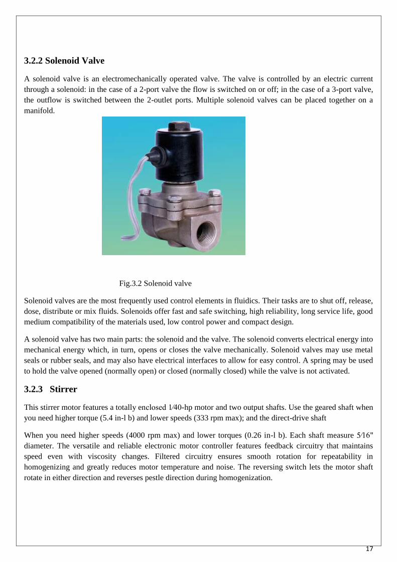
3.2.2 Solenoid Valve

A solenoid valve is an electromechanically operated valve. The valve is controlled by an electric current

through a solenoid: in the case of a 2-port valve the flow is switched on or off; in the case of a 3-port valve,

the outflow is switched between the 2-outlet ports. Multiple solenoid valves can be placed together on a

manifold.

Fig.3.2 Solenoid valve

Solenoid valves are the most frequently used control elements in fluidics. Their tasks are to shut off, release,

dose, distribute or mix fluids. Solenoids offer fast and safe switching, high reliability, long service life, good

medium compatibility of the materials used, low control power and compact design.

A solenoid valve has two main parts: the solenoid and the valve. The solenoid converts electrical energy into

mechanical energy which, in turn, opens or closes the valve mechanically. Solenoid valves may use metal

seals or rubber seals, and may also have electrical interfaces to allow for easy control. A spring may be used

to hold the valve opened (normally open) or closed (normally closed) while the valve is not activated.

3.2.3 Stirrer

This stirrer motor features a totally enclosed 1⁄40-hp motor and two output shafts. Use the geared shaft when

you need higher torque (5.4 in-l b) and lower speeds (333 rpm max); and the direct-drive shaft

When you need higher speeds (4000 rpm max) and lower torques (0.26 in-l b). Each shaft measure 5⁄16"

diameter. The versatile and reliable electronic motor controller features feedback circuitry that maintains

speed even with viscosity changes. Filtered circuitry ensures smooth rotation for repeatability in

homogenizing and greatly reduces motor temperature and noise. The reversing switch lets the motor shaft

rotate in either direction and reverses pestle direction during homogenization.

18

3.2.4 DC Motor

A DC motor is a mechanically commutated electric motor powered from direct current (DC). The stator is

stationary in space by definition and therefore so is its current. The current in the rotor is switched by the

commutator to also be stationary in space. This is how the relative angle between the stator and rotor

magnetic flux is maintained near 90 degrees, which generates the maximum torque.

DC motors have a rotating armature winding but non-rotating armature magnetic field and a static field

winding or permanent magnet. Different connections of the field and armature winding provide different

inherent speed/torque regulation characteristics. The speed of a DC motor can be controlled by changing the

voltage applied to the armature or by changing the field current. The introduction of variable resistance in

the armature circuit or field circuit allowed speed control. Modern DC motors are often controlled by power

electronics systems called DC drives.

Fig.3.3 DC motor

The introduction of DC motors to run machinery eliminated the need for local steam or internal combustion

engines, and line shaft drive systems. DC motors can operate directly from rechargeable batteries, providing

the motive power for the first electric vehicles. Today DC motors are still found in applications as small as

toys and disk drives, or in large sizes to operate steel rolling mills and paper machines.

Connection types

There are three types of electrical connections between the stator and rotor possible for DC electric motors:

series, shunt/parallel and compound (various blends of series and shunt/parallel) and each has unique

speed/torque characteristics appropriate for different loading torque profiles/signatures.

Series connection

A series DC motor connects the armature and field windings in series with a common D.C. power source.

The motor speed varies as a non-linear function of load torque and armature current; current is common to

both the stator and rotor yielding I^2 (current) squared behavior.

A series motor has very high starting torque and is commonly used for starting high inertia loads, such as

trains, elevators or hoists. This speed/torque characteristic is useful in applications such as dragline

excavators, where the digging tool moves rapidly when unloaded but slowly when carrying a heavy load.

19

With no mechanical load on the series motor, the current is low, the counter-EMF produced by the field

winding is weak, and so the armature must turn faster to produce sufficient counter-EMF to balance the

supply voltage. The motor can be damaged by over speed. This is called a runaway condition.

Series motors called "universal motors" can be used on alternating current. Since the armature voltage and

the field direction reverse at (substantially) the same time, torque continues to be produced in the same

direction. Since the speed is not related to the line frequency, universal motors can develop higher-than-

synchronous speeds, making them lighter than induction motors of the same rated mechanical output. This is

a valuable characteristic for hand-held power tools. Universal motors for commercial power frequency are

usually small, not more than about 1 kW output. However, much larger universal motors were used for

electric locomotives, fed by special low-frequency traction power networks to avoid problems with

commutation under heavy and varying loads.

Shunt connection

A shunt DC motor connects the armature and field windings in parallel or shunt with a common D.C. power

source. This type of motor has good speed regulation even as the load varies, but does not have as high of

starting torque as a series DC motor. It is typically used for industrial, adjustable speed applications, such as

machine tools, winding/unwinding machines and tensioners.

Compound connection

R vs T relationship of various metals

Common RTD sensing elements constructed of platinum, copper or nickel have a unique, and

repeatable and predictable resistance versus temperature relationship (R vs T) and operating temperature

range. The R vs T relationship is defined as the amount of resistance change of the sensor per degree of

temperature change. The relative change in resistance (temperature coefficient of resistance) varies only

slightly over the useful range of the sensor.

Platinum is a noble metal and has the most stable resistance-temperature relationship over the

largest temperature range. Nickel elements have a limited temperature range because the amount of change

in resistance per degree of change in temperature becomes very non-linear at temperatures over 572 °F

(300 °C). Copper has a very linear resistance-temperature relationship, however copper oxidizes at

moderate temperatures and cannot be used over 302 °F (150 °C).

Platinum is the best metal for RTDs because it follows a very linear resistance-temperature

relationship and it follows the R vs T relationship in a highly repeatable manner over a wide temperature

range. The unique properties of platinum make it the material of choice for temperature standards over the

range of -272.5 °C to 961.78 °C, and is used in the sensors that define the International Temperature

Standard, ITS-90. Platinum is chosen also because of its chemical inertness.

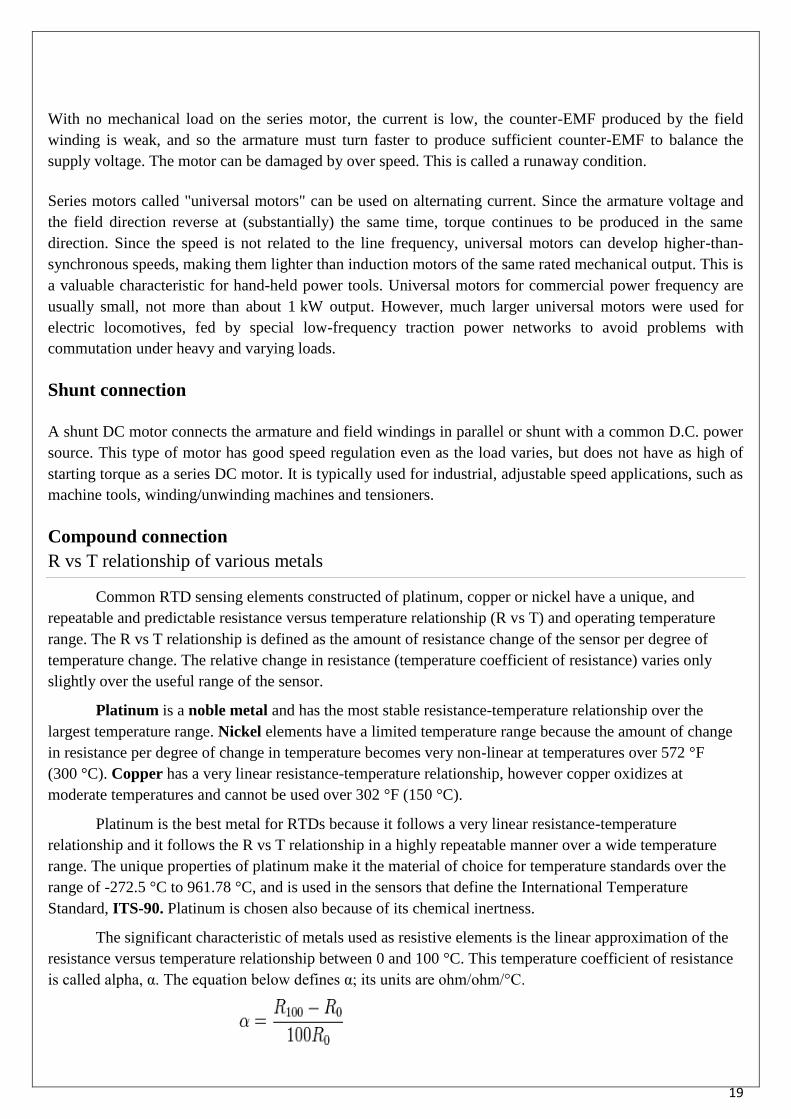
The significant characteristic of metals used as resistive elements is the linear approximation of the

resistance versus temperature relationship between 0 and 100 °C. This temperature coefficient of resistance

is called alpha, α. The equation below defines α; its units are ohm/ohm/°C.

20

The resistance of the sensor at 0°C

The resistance of the sensor at 100°C

Pure platinum has an alpha of 0.003925 ohm/ohm/°C and is used in the construction of laboratory

grade RTDs. Conversely two widely recognized standards for industrial RTDs IEC 60751 and ASTM E-

1137 specify an alpha of 0.00385 ohms/ohm/°C. Before these standards were widely adopted several

different alpha values were used. It is still possible to find older probes that are made with platinum that

have alpha values of 0.003916 ohms/ohm/°C and 0.003902 ohms/ohm/°C.

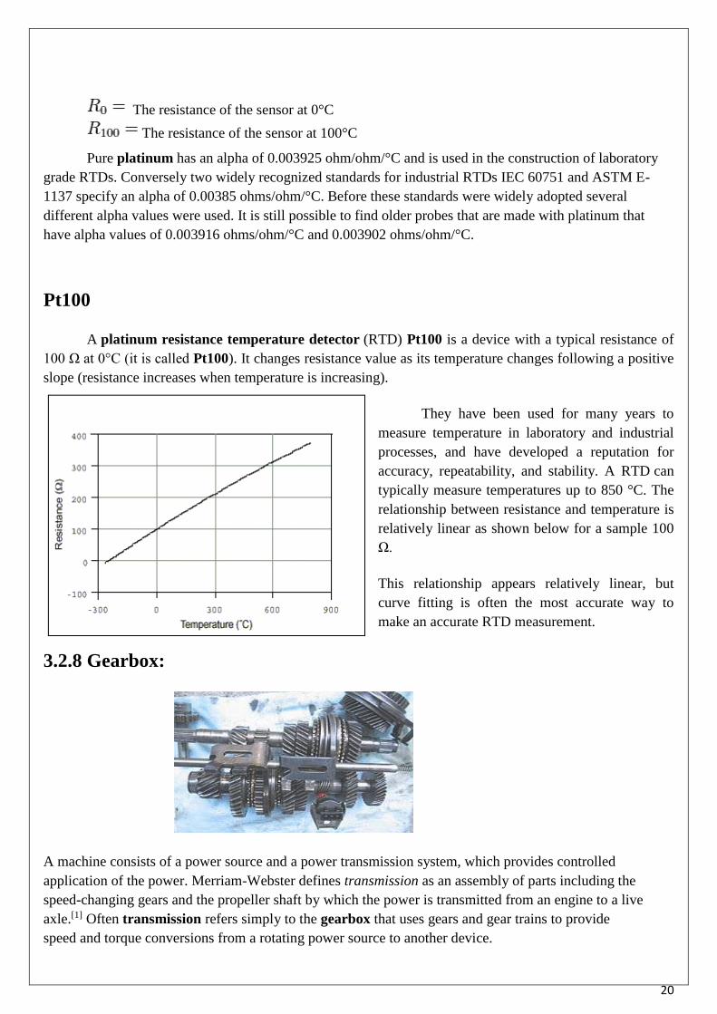
Pt100

A platinum resistance temperature detector (RTD) Pt100 is a device with a typical resistance of

100 Ω at 0°C (it is called Pt100). It changes resistance value as its temperature changes following a positive

slope (resistance increases when temperature is increasing).

They have been used for many years to

measure temperature in laboratory and industrial

processes, and have developed a reputation for

accuracy, repeatability, and stability. A RTD can

typically measure temperatures up to 850 °C. The

relationship between resistance and temperature is

relatively linear as shown below for a sample 100

Ω.

This relationship appears relatively linear, but

curve fitting is often the most accurate way to

make an accurate RTD measurement.

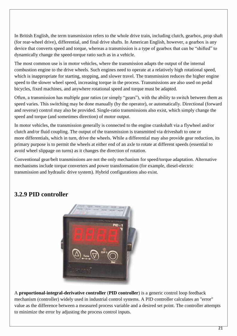
3.2.8 Gearbox:

A machine consists of a power source and a power transmission system, which provides controlled

application of the power. Merriam-Webster defines transmission as an assembly of parts including the

speed-changing gears and the propeller shaft by which the power is transmitted from an engine to a live

axle.[1] Often transmission refers simply to the gearbox that uses gears and gear trains to provide

speed and torque conversions from a rotating power source to another device.

21

In British English, the term transmission refers to the whole drive train, including clutch, gearbox, prop shaft

(for rear-wheel drive), differential, and final drive shafts. In American English, however, a gearbox is any

device that converts speed and torque, whereas a transmission is a type of gearbox that can be “shifted” to

dynamically change the speed-torque ratio such as in a vehicle.

The most common use is in motor vehicles, where the transmission adapts the output of the internal

combustion engine to the drive wheels. Such engines need to operate at a relatively high rotational speed,

which is inappropriate for starting, stopping, and slower travel. The transmission reduces the higher engine

speed to the slower wheel speed, increasing torque in the process. Transmissions are also used on pedal

bicycles, fixed machines, and anywhere rotational speed and torque must be adapted.

Often, a transmission has multiple gear ratios (or simply “gears”), with the ability to switch between them as

speed varies. This switching may be done manually (by the operator), or automatically. Directional (forward

and reverse) control may also be provided. Single-ratio transmissions also exist, which simply change the

speed and torque (and sometimes direction) of motor output.

In motor vehicles, the transmission generally is connected to the engine crankshaft via a flywheel and/or

clutch and/or fluid coupling. The output of the transmission is transmitted via driveshaft to one or

more differentials, which in turn, drive the wheels. While a differential may also provide gear reduction, its

primary purpose is to permit the wheels at either end of an axle to rotate at different speeds (essential to

avoid wheel slippage on turns) as it changes the direction of rotation.

Conventional gear/belt transmissions are not the only mechanism for speed/torque adaptation. Alternative

mechanisms include torque converters and power transformation (for example, diesel-electric

transmission and hydraulic drive system). Hybrid configurations also exist.

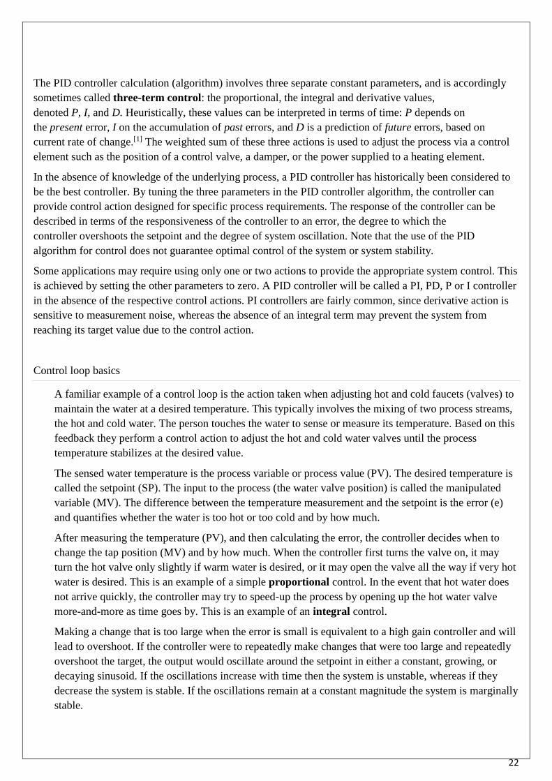
3.2.9 PID controller

A proportional-integral-derivative controller (PID controller) is a generic control loop feedback

mechanism (controller) widely used in industrial control systems. A PID controller calculates an "error"

value as the difference between a measured process variable and a desired set point. The controller attempts

to minimize the error by adjusting the process control inputs.

22

The PID controller calculation (algorithm) involves three separate constant parameters, and is accordingly

sometimes called three-term control: the proportional, the integral and derivative values,

denoted P, I, and D. Heuristically, these values can be interpreted in terms of time: P depends on

the present error, I on the accumulation of past errors, and D is a prediction of future errors, based on

current rate of change.[1] The weighted sum of these three actions is used to adjust the process via a control

element such as the position of a control valve, a damper, or the power supplied to a heating element.

In the absence of knowledge of the underlying process, a PID controller has historically been considered to

be the best controller. By tuning the three parameters in the PID controller algorithm, the controller can

provide control action designed for specific process requirements. The response of the controller can be

described in terms of the responsiveness of the controller to an error, the degree to which the

controller overshoots the setpoint and the degree of system oscillation. Note that the use of the PID

algorithm for control does not guarantee optimal control of the system or system stability.

Some applications may require using only one or two actions to provide the appropriate system control. This

is achieved by setting the other parameters to zero. A PID controller will be called a PI, PD, P or I controller

in the absence of the respective control actions. PI controllers are fairly common, since derivative action is

sensitive to measurement noise, whereas the absence of an integral term may prevent the system from

reaching its target value due to the control action.

Control loop basics

A familiar example of a control loop is the action taken when adjusting hot and cold faucets (valves) to

maintain the water at a desired temperature. This typically involves the mixing of two process streams,

the hot and cold water. The person touches the water to sense or measure its temperature. Based on this

feedback they perform a control action to adjust the hot and cold water valves until the process

temperature stabilizes at the desired value.

The sensed water temperature is the process variable or process value (PV). The desired temperature is

called the setpoint (SP). The input to the process (the water valve position) is called the manipulated

variable (MV). The difference between the temperature measurement and the setpoint is the error (e)

and quantifies whether the water is too hot or too cold and by how much.

After measuring the temperature (PV), and then calculating the error, the controller decides when to

change the tap position (MV) and by how much. When the controller first turns the valve on, it may

turn the hot valve only slightly if warm water is desired, or it may open the valve all the way if very hot

water is desired. This is an example of a simple proportional control. In the event that hot water does

not arrive quickly, the controller may try to speed-up the process by opening up the hot water valve

more-and-more as time goes by. This is an example of an integral control.

Making a change that is too large when the error is small is equivalent to a high gain controller and will

lead to overshoot. If the controller were to repeatedly make changes that were too large and repeatedly

overshoot the target, the output would oscillate around the setpoint in either a constant, growing, or

decaying sinusoid. If the oscillations increase with time then the system is unstable, whereas if they

decrease the system is stable. If the oscillations remain at a constant magnitude the system is marginally

stable.

23

In the interest of achieving a gradual convergence at the desired temperature (SP), the controller may

wish to damp the anticipated future oscillations. So in order to compensate for this effect, the controller

may elect to temper its adjustments. This can be thought of as a derivative control method.

If a controller starts from a stable state at zero error (PV = SP), then further changes by the controller

will be in response to changes in other measured or unmeasured inputs to the process that impact on the

process, and hence on the PV. Variables that impact on the process other than the MV are known as

disturbances. Generally controllers are used to reject disturbances and/or implement setpoint changes.

Changes in feedwater temperature constitute a disturbance to the faucet temperature control process.

In theory, a controller can be used to control any process which has a measurable output (PV), a known

ideal value for that output (SP) and an input to the process (MV) that will affect the relevant PV.

Controllers are used in industry to regulate temperature, pressure, flow

rate, chemical composition, speed and practically every other variable for which a measurement exists.

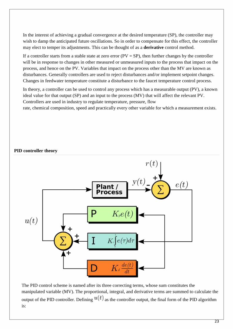
PID controller theory

The PID control scheme is named after its three correcting terms, whose sum constitutes the

manipulated variable (MV). The proportional, integral, and derivative terms are summed to calculate the

output of the PID controller. Defining as the controller output, the final form of the PID algorithm

is:

24

Where

: Proportional gain, a tuning parameter

: Integral gain, a tuning parameter

: Derivative gain, a tuning parameter

: Error

: Time or instantaneous time (the present)

: Variable of integration; takes on values from time 0 to the present .

Proportional term:

Plot of PV vs time, for three values of Kp (Ki and

Kd held constant)

The proportional term produces an output value that is

proportional to the current error value. The proportional

response can be adjusted by multiplying the error by a

constant Kp, called the proportional gain constant.

The proportional term is given by:

A high proportional gain results in a large change in the

output for a given change in the error. If the proportional

gain is too high, the system can become unstable

(see the section on loop tuning). In contrast, a small gain results in a small output response to a large input

error, and a less responsive or less sensitive controller. If the proportional gain is too low, the control action

may be too small when responding to system disturbances. Tuning theory and industrial practice indicate

that the proportional term should contribute the bulk of the output change.

Droop

Because a non-zero error is required to drive it, a proportional controller generally operates with a steady-

state error, referred to as droop. Droop is proportional to the process gain and inversely proportional to

proportional gain. Droop may be mitigated by adding a compensating bias term to the setpoint or output, or

corrected dynamically by adding an integral term.

25

Integral term

Plot of PV vs time, for three values of Ki (Kp and d held

constant)

The contribution from the integral term is proportional

to both the magnitude of the error and the duration of

the error. The integral in a PID controller is the sum of

the instantaneous error over time and gives the

accumulated offset that should have been corrected

previously. The accumulated error is then multiplied by

the integral gain ( ) and added to the controller

output.The integral term is given by:

The integral term accelerates the movement of the process towards setpoint and eliminates the residual

steady-state error that occurs with a pure proportional controller. However, since the integral term responds

to accumulated errors from the past, it can cause the present value to overshoot the setpoint value (see the

section on loop tuning).

Derivative term

Plot of PV vs time, for three values of Kd (Kp and

Ki held constant)

The derivative of the process error is calculated by

determining the slope of the error over time and

multiplying this rate of change by the derivative

gain . The magnitude of the contribution of the

derivative term to the overall control action is termed

the derivative gain, .

The derivative term is given by:

Derivative action predicts system behavior and thus improves settling time and stability of the system.

Loop tuning

Tuning a control loop is the adjustment of its control parameters (proportional band/gain, integral gain/reset,

derivative gain/rate) to the optimum values for the desired control response. Stability (bounded oscillation)

is a basic requirement, but beyond that, different systems have different behavior, different applications have

different requirements, and requirements may conflict with one another.

26

PID tuning is a difficult problem, even though there are only three parameters and in principle is simple to

describe, because it must satisfy complex criteria within the limitations of PID control. There are

accordingly various methods for loop tuning, and more sophisticated techniques are the subject of patents;

this section describes some traditional manual methods for loop tuning.

Designing and tuning a PID controller appears to be conceptually intuitive, but can be hard in practice, if

multiple (and often conflicting) objectives such as short transient and high stability are to be achieved.

Usually, initial designs need to be adjusted repeatedly through computer simulations until the closed-loop

system performs or compromises as desired.

Some processes have a degree of nonlinearity and so parameters that work well at full-load conditions don't

work when the process is starting up from no-load; this can be corrected by gain scheduling (using different

parameters in different operating regions). PID controllers often provide acceptable control using default

tunings, but performance can generally be improved by careful tuning, and performance may be

unacceptable with poor tuning.

Stability

If the PID controller parameters (the gains of the proportional, integral and derivative terms) are chosen

incorrectly, the controlled process input can be unstable, i.e., its output diverges, with or without oscillation,

and is limited only by saturation or mechanical breakage. Instability is caused by excess gain, particularly in

the presence of significant lag.

Generally, stabilization of response is required and the process must not oscillate for any combination of

process conditions and setpoints, though sometimes marginal stability (bounded oscillation) is acceptable or

desired.

3.2.11 ABB MCB:

MCB´s protect installations against overload and short-circuit, warranting reliability and safety for

operations.

New System pro M compact S200 series are current limiting overcurrent protective devices. They have two

different tripping mechanisms, the delayed thermal tripping mechanism for overload protection and the

magnetic tripping mechanism for short circuit protection. They are available in different characteristics (B,

C, D, K, Z), configurations (1P, 1P+N, 2P, 3P, 3P+N, 4P), breaking capacities (up to 25 kA) and rated

currents (up to 63A). Depending on the product range, New System pro M compact S200 series comply

with

• IEC/EN 60898-1

27

• IEC/EN 60947-2

• UL 1077

• UL 489

allowing the use for residential, commercial and industrial applications.

Miniature circuit breakers (MCBs)

For domestic/residential installations in defined markets up to 6 kA breaking capacity 3 / 4 / 5 / 6 kA

• Compact Home SH 200 T, SH 200 L, SH 200

For domestic or small commercial installations up to 10 kA breaking capacity

• pro M compact S200, S200S, S200 M

For industrial installations up to 25 kA breaking capacity

• pro M compact S200, S200M, S200P, S200U, S200UP, S200UDC

• S280UC, S290

For commercial and industrial applications with high breaking capacities and special features / accessories

• S200P, S220, S290

• S500, S800

Special selective MCB (SMCB) with dedicated upstream and downstream selectivity are available in the

ranges

• S700

• S750

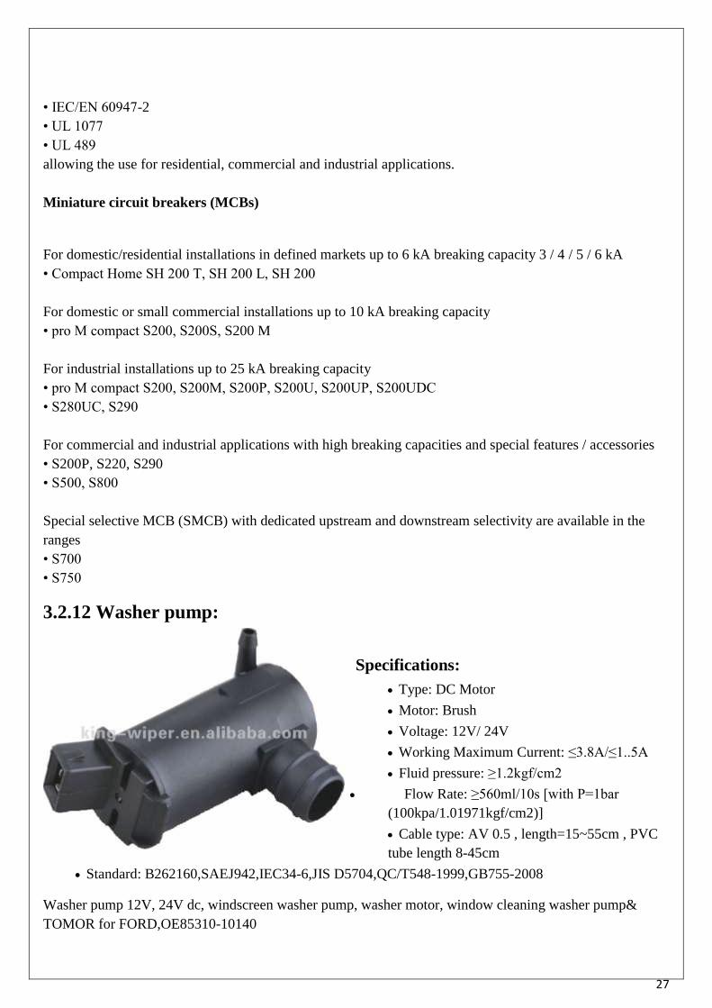
3.2.12 Washer pump:

Specifications:

Type: DC Motor

Motor: Brush

Voltage: 12V/ 24V

Working Maximum Current: ≤3.8A/≤1..5A

Fluid pressure: ≥1.2kgf/cm2

Flow Rate: ≥560ml/10s [with P=1bar

(100kpa/1.01971kgf/cm2)]

Cable type: AV 0.5 , length=15~55cm , PVC

tube length 8-45cm

Standard: B262160,SAEJ942,IEC34-6,JIS D5704,QC/T548-1999,GB755-2008

Washer pump 12V, 24V dc, windscreen washer pump, washer motor, window cleaning washer pump&

TOMOR for FORD,OE85310-10140

28

29

30

3.2.13 Three Pole Power Contactors - Type MNX 12

Catalogue No. CS 94108 / 9*

Power Contacts

No. of poles 3

Rated insulation voltage, Ui 690V

Rated impulse withstand voltage, Ui 8 kV

Rated making capacity - Amp 450

Rated breaking capacity - Amp 250

Conventional thermal current,

Ith

At 550C

Motor duty : 3Ø, 415V, 50Hz

30A Utilization category AC-

1 12A Utilization category AC-

2 5.5kW / 7.5hp / 12A Utilization category AC-

3 5.5kW / 7.5hp / 12A Utilization category AC-

4 Operational current /e for AC-4 Utilization

category at 415V,3Ø, 5OHz for 2,00,000

operating cycles

7.1A

Capacitor switching delta connected: 415V, 50Hz *** 7.5 k VAR Max. Permissible peak in-rush current, /p for capacitor

switching

680A

DC ratings (with 3 poles in

series)

and AC coil operation

12A DC 1 - 110V 12A DC 1 - 220V 12A DC 3 - 110V 12A DC 3 - 220V 12A DC 5 - 110V 7.5A DC 5 - 220V

Mechanical life, No. of operating cycles 15x106

Max. frequency of

operations: Operating

cycles/hr

7200 Mechanical 3000 Utilization Category

AC-1 750 Utilization Category

AC-2 750 Utilization Category

AC-3 300 Utilization Category

AC-4 Service Temperature -200C to +550C

Main terminal capacity

1 x 6 Lug (mm2)

- Link (mm2)

2 x 4 Solid Conductors (mm2)

2 x 2.5 Multi strand conductors

(mm2) Auxiliary Contacts

No. of built-in auxiliary contacts 1NO or 1NC

Conventional thermal current, / at 550C

t

h

10A

AC-15 rating at 415V, 50Hz 4A

Terminal capacity (Solid or multi strand conductors (mm2) 2 x 2.5

Coil

Voltage available for 50 Hz Uc V 24, 42, 110,

220 / 240, 415, 525 Pick-up 68 VA 0.82 Cos Ø Hold-on 11 VA 4 Watts Limits of operation 65 - 120 Pick-up (%Uc) 35 - 65 Drop-off(%Uc)

31

3.2.14 UNISON SSR

801 MODEL

DC TO AC SOLID STATE RELAY

(BACK TO BACK SCR & TRIAC)

INPUT: 4VDC TO 32VDC, 4-16mA,

OUTPUT : 24 TO 330VAC /480VAC,

25Amp / 50Amp / 90Amp / 150Amp, 1200PIV/1600PIV

32

Chapter 4

Actual Work Done

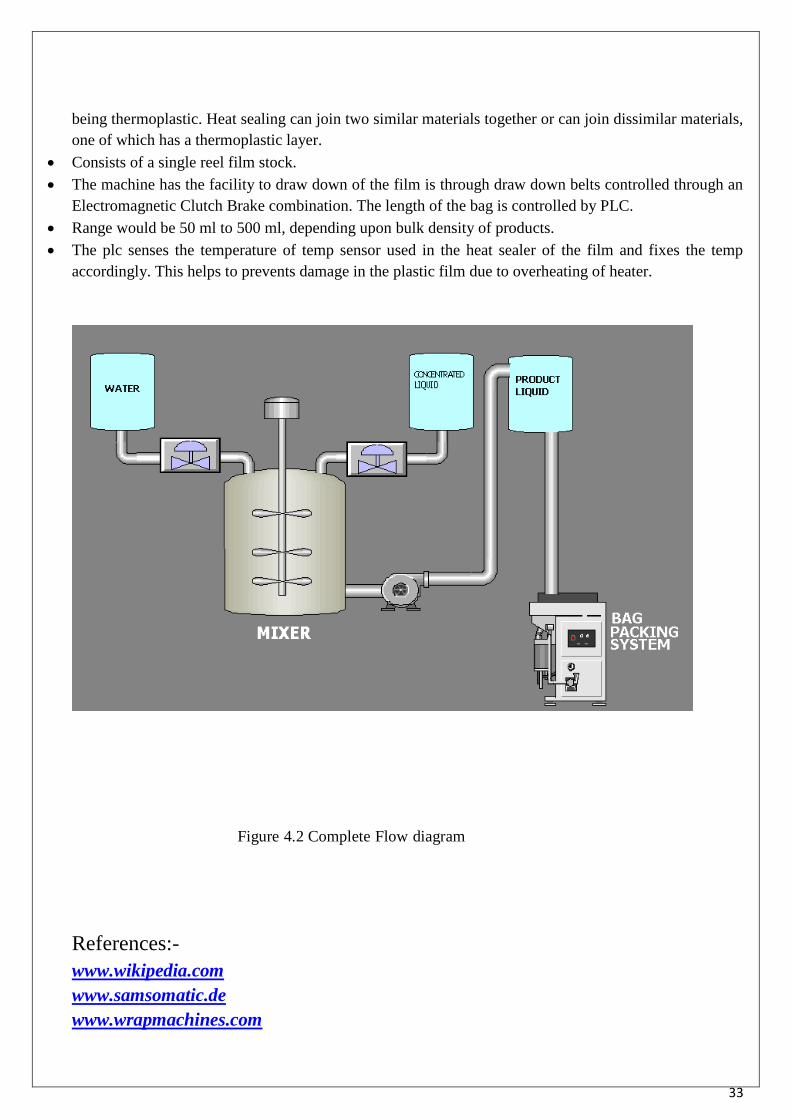
4.1 Liquid Mixing Process System

As our Project is to mix the concentrated liquid and water using the stirrer to get the product of

beverages liquid. Then further, the liquid is packed in plastic bag.

As shown in the diagram, two plastic containers have been used wherein the two separate liquids to

be mixed would be stored, as the process proceeds the two liquids would be mixed in a mixing tank

where the both liquids from the previous two containers will be poured in. After the mixing

procedure finishes, the resultant mixed liquid will be sent to the main SS storage tank where it would

be stored until the packing procedure initiates.

The plc interface coding which handle the automatic operation of the mixing procedure is done in the

ladder diagram language.

PLC controls the flow of the solenoid valve as well as the continuous valve. It controls the flow

value of concentrated and the water required proportion on the time duration basis.

4.2 Bag packing system

The basic feature of a pouch packing machine is the packaging accuracy which results in the perfect

weight, size and cut of the pouches. The pouch packing machine is engineered in such a way that they

exceed all quality standards. They make use of advanced technology to produce effective and reliable

products. The pouch packing machine provides an ideal sealing solution in view of the fact that they use

the heat sealing system. The pouch packing machine helps to fill pouches, seal them and cut them as

well. All of this happens in one continuous operation on the pouch packing machine. The pouch packing

machine is particularly very important for manufacturers who produce liquid or powder-based products.

In the packing procedure the plastic film is first center folded and made into a holding pouch into which

the mixed liquid is poured into, after which the pouch is sealed to make a single pouched unit, and this

process continues depending upon the number of units to be pouched.

After the mixing of the liquid, the packing system will pack liquid in plastic bag.

A vertical form, fill and seal machine for producing center sealed pouches handling all types of free

flowing liquids.

A heat sealer would be used to seal products, packaging, and other thermoplastic materials using heat.

This can be with uniform thermoplastic monolayers or with materials having several layers, at least one

33

being thermoplastic. Heat sealing can join two similar materials together or can join dissimilar materials,

one of which has a thermoplastic layer.

Consists of a single reel film stock.

The machine has the facility to draw down of the film is through draw down belts controlled through an

Electromagnetic Clutch Brake combination. The length of the bag is controlled by PLC.

Range would be 50 ml to 500 ml, depending upon bulk density of products.

The plc senses the temperature of temp sensor used in the heat sealer of the film and fixes the temp

accordingly. This helps to prevents damage in the plastic film due to overheating of heater.

Figure 4.2 Complete Flow diagram

References:-

www.wikipedia.com

www.samsomatic.de

www.wrapmachines.com