mixed effects models methods and classes for s and splus ...sun.cwru.edu/~jiayang/nlme.pdf ·...

lme and nlme

Mixed Effects Models Methods and Classes for S and SplusVersion 1.2

February 1995

by Jose C. Pinheiro and Douglas M. Bates

University of Wisconsin — Madison

lme and nlme: Mixed-effects Methods and Classes for S and S-plus

Mixed-effects models provide a powerful and flexible tool for analyzing clustered data, such as

repeated measures data and nested designs.

We describe a set of S functions, classes, and methods for the analysis of both linear and non-

linear mixed-effects models. These extend the linear and nonlinear modeling facilities available in

release 3 of S and S-plus. The source code, written in S and C is available in the S collection at

StatLib. Help files for all functions and methods described here are included in Appendix A.

Jose C. [email protected]

Douglas M. [email protected]

Contents

1 Introduction 1

2 The lme class and related methods 12.1 The lme function : : : : : : : : : : : : : : : : : : : : : : : : : : : : : : : : : 22.2 The print, summary, and anova methods. : : : : : : : : : : : : : : : : : : 22.3 The plot method : : : : : : : : : : : : : : : : : : : : : : : : : : : : : : : : : 42.4 Other methods : : : : : : : : : : : : : : : : : : : : : : : : : : : : : : : : : : : 62.5 Structured variance-covariance matrices and random effects blocks : : : : : : : : 6

3 The nlme class and related methods 103.1 The nlme function : : : : : : : : : : : : : : : : : : : : : : : : : : : : : : : : 113.2 Methods for nlme objects : : : : : : : : : : : : : : : : : : : : : : : : : : : : : 123.3 Structured variance-covariance matrices and random effects blocks : : : : : : : : 16

4 Future Developments 16

Appendix A: Help Files 18

Mixed effects methods and classes for S and S-plus 1

1 Introduction

Mixed-effects models provide a powerful and flexible tool for analyzing clustered data, such as repeated measures dataand nested designs. We describe a set of S functions, classes, and methods for the analysis of linear or nonlinear mixed-effects models. These extend the linear and nonlinear modeling facilities available in release 3 of S (Chambers andHastie, 1992) and S-plus.

The source code, written in S and C, is available in the S collection at StatLib. It can be obtained either throughelectronic mail, by sending the one-line message send nlme from S to the address [email protected], orvia anonymous ftp from ftp://lib.stat.cmu.edu/S/nlme or ftp://ftp.stat.wisc.edu/src/NLME/Unix.The StatLib version of the code is intended for Unix based machines. A MicroSoft Windows version for S-plus ver-sion 3.2 is available for anonymous ftp from ftp://ftp.stat.wisc.edu/src/NLME/Windows. Help files for allfunctions and methods described here can be found in Appendix A.

Section 2 presents the functions and methods for fitting and analyzing linear mixed-effects models. The nonlinearmixed-effects functions and methods are described in section 3. Section 4 presents some future directions for the codedevelopment.

2 The lme class and related methods

Fitting and analyzing linear mixed-effects models will be described here. First we consider the data from a den-tal study presented in Potthoff and Roy (1964). The data, dis-played in Figure 1, consist of four measurements of the dis-tance (in millimeters) from the center of the pituitary to thepteryomaxillary fissure made at ages 8, 10, 12, and 14 yearson 16 boys and 11 girls. A linear model seems adequate to ex-plain the distance as a function of age, but the intercept and theslope seem to vary with the individual. The corresponding lin-ear mixed-effects model isdij = (�0 + bi0) + (�1 + bi1) agej + "ij ; (1)where dij represents the distance for the ith individual at agej, �0 and �1 are the population average intercept and the popu-lation average slope, bi0 and bi1 are the effects in intercept andslope associated with the ith individual, and "ij is the within-subject error term. It is assumed that the bi = (bi0; bi1)T areindependent and identically distributed with a N(0; �2D) dis-tributionand the "ij are independent and identically distributedwith a N(0; �2) distribution, independent of the bi. Age (years)

Dis

tanc

e (m

m)

8 9 10 11 12 13 14

20

25

30

Boys

Girls

Figure 1: Distance from the center of the pituitary to the ptery-omaxillary fissure in boys and girls at different ages.

One of the questions of interest for these data is whether these curves show significant differences between boys andgirls. Model (1) can be modified asdij = (�00 + �01sexi + bi0) + (�10 + �11sexi + bi1) agej + "ij (2)

to test for sex related differences in intercept and slope. In model (2), sexi is an indicator variable assuming value zeroif the ith individual is a boy and one if she is a girl. �00 and �10 represent the population average intercept and slopefor the boys and �01 and �11 are the changes in population average intercept and slope for girls. Differences betweenboys and girls can be evaluated by testing whether �01 and �11 are significantly different from zero. The remainingterms in (2) are defined as in (1). It will be assumed here that the data are available in a data frame called dental, withcolumns distance, age, subject, and sex as below.


> dentaldistance age subject sex

1 26.0 8 1 02 25.0 10 1 03 29.0 12 1 04 31.0 14 1 0

. . .105 24.5 8 27 1106 25.0 10 27 1107 28.0 12 27 1108 28.0 14 27 1

2.1 The lme function

The lme function is used to fit a linear mixed-effects model, as described in Laird and Ware (1982), using either maxi-mum likelihood or restricted maximum likelihood. It produces an object of class lme. Several optional arguments canbe used with this function, but the typical call is

lme(fixed, random, cluster, data)

The first three arguments are required. The arguments fixed and random are formulas as shown below. Any linearmodel formula (Chambers and Hastie, 1992, chapter 3) is allowed, giving the model formulation considerable flexibil-ity. For the dental data these formulas would be written as

fixed = distance ˜ age, random = ˜ age

for model (1) and

fixed = distance ˜ age * sex, random = ˜ age

for model (2). Note that the response variable is given only in the formula for the fixed argument.The cluster argument is a formula, or expression, defining the labels for the different subjects in the data. For

the dental data we would use

cluster = ˜ subject

for both models (1) and (2). The optional argument data specifies the data frame in which the variables used in themodel are available. A simple call to lme to fit model (1) would be

> dental.fit1 <- lme(fixed = distance ˜ age, random = ˜ age,+ cluster = ˜ subject, data = dental)

To fit model (2) we would use

> dental.fit2 <- lme(fixed = distance ˜ age * sex, random = ˜ age,+ cluster =˜ subject, data = dental)

There are several methods available for the fitted objects of class lme, including those for the generic functionsprint, summary, and plot.

2.2 The print, summary, and anova methods.

A brief description of the estimation results is returned by the print method. It gives estimates of the standard errorsand correlations of the random effects, the cluster variance, and the fixed effects. For the dental.fit1 object we get

> dental.fit1Call:

Fixed: distance ˜ ageRandom: ˜ ageCluster: ˜ subject

Data: dental


Variance/Covariance Components Estimates:

Structure: unstructuredParametrization: logcholeskyStandard Deviation(s) of Random Effect(s)

(Intercept) age2.194103 0.2149245

Correlation of Random Effects(Intercept)

age -0.5814881

Cluster Residual Variance: 1.716204

Fixed Effects Estimates:(Intercept) age

16.76111 0.6601852

Number of Observations: 108Number of Clusters: 27

A more complete description of the estimation results is returned by summary.

> summary(dental.fit2). . .Loglikelihood: -114.6576AIC: 245.3152

Variance/Covariance Components Estimates:Structure: unstructuredParametrization: logcholeskyStandard Deviation(s) of Random Effect(s)

(Intercept) age2.134464 0.1541247

Correlation of Random Effects(Intercept)

age -0.6024329


Fixed Effects Estimates:Value Approx. Std.Error z ratio(C)

(Intercept) 16.3406250 0.98005731 16.6731321age 0.7843750 0.08275189 9.4786353sex 1.0321023 1.53545472 0.6721802

age:sex -0.3048295 0.12964730 -2.3512218

Conditional Correlations of Fixed Effects Estimates(Intercept) age sex

age -0.8801554sex -0.6382847 0.5617897

age:sex 0.5617897 -0.6382847 -0.8801554. . .

The approximate standard errors for the fixed effects are derived using the asymptotic theory described in Pinheiro(1994). The results above indicate that the measurement increases faster in boys than in girls (significant, negativeage:sex fixed effect), but the average intercept is common to boys and girls (non-significant sex fixed effect).

A likelihood ratio test to evaluate the hypothesis of no sex differences in distance development is given by theanovamethod.


> anova(dental.fit1, dental.fit2). .

Model Df AIC Loglik Test Lik.Ratio P valuedental.fit1 1 6 252.72 -120.36dental.fit2 2 8 245.32 -114.66 1 vs. 2 11.406 0.0033365

The likelihood ratio test strongly rejects the null hypothesis of no sex differences. To use a likelihood test to test if thegrowth rate only is dependent on sex we fit

> dental.fit3 <- lme(fixed = distance ˜ age + age:sex, random = ˜ age,+ cluster = ˜ subject, data = dental)

and use the anova method again.

> anova(dental.fit2, dental.fit3). . .

Model Df AIC Loglik Test Lik.Ratio P valuedental.fit2 1 8 245.32 -114.66dental.fit3 2 7 243.76 -114.88 1 vs. 2 0.44806 0.50326

As expected, the likelihood ratio test indicates that the initial distances do not depend on sex.

2.3 The plot method

Plots of random effects estimates, residuals, and fitted values can be obtained using the plot method for class lme.The following call will produce a scatter plot of the estimated random effects for intercept and slope in model (2), asshown in Figure 2.> plot(dental.fit2, pch = "o")

The point at the upper left corner of Figure 2 appears to be anoutlying value that could have a great impact on the correla-tion and variance estimates.

Residual plots may be obtained by setting the argumentoption in the plot method to "r".> par(mfrow = c(2, 2))

> plot(dental.fit3, option = "r", pch = "o")

The resulting plots are included in Figure 3. The first plot, ob-served versus fitted values, indicates that the linear model doesa reasonable job of explaining the distance growth. The pointsfall relatively close to the y = x line, indicating a reasonableagreement between the fitted and observed values. The sec-ond plot, residuals versus fitted values, suggests the presenceof three outliers in the data. The remaining residuals appear tobe homogeneously scattered around the y = 0 line. The finalplot, featuring the boxplot of the residuals by subject, suggests

o

oo

o

oo

o

o

o

o

o

o

o

o

o

o

o

o

o

o

oo

o

ooo

o

(Intercept)

age

-3 -2 -1 0 1 2 3

-0.1

0.0

0.1

0.2

Figure 2: Scatter plot of the conditional modes of the interceptand slope random effects in model (2).

that the outliers occurred for subjects 9 and 13. There seems to be considerable variation in the within-subject variabil-ity, but it must be remembered that each of the boxplots represent only four residuals.


oo

o

o

oo

o

o

oo

o

o

o

oo

o

o

oo

o

oo

o

o

o o

o

o

o

o

oo

o

o

o

o

oo

oo

o oo

o

o

oo

o

o

o

o

o

o

o oo

o

o

o

o

oo

o

o

oo

o

o

oo

o

o

o

oo

o

oo

o

o

o

oo

o

oo o

oo

oo

o

o oo

o

oo

oo

o

o oo

oo

o o

Fitted Values

Obs

erve

d V

alue

s

18 20 22 24 26 28 30 32

20

25

30

o

o

oo

oo

o

oo

o o

oo

o

o

oo

o

o

ooo o o

o

o

oo

o

o

oo

o

o

o

o

o

o

o

o

o

o

o oo

o

o

o

o

oo

o

o

o

o

o

o o o

o

o

oo o

o

oo

oo

o

oo

o

oo

oo oo

ooo

o oo o

ooo o

o

oo

oo

oo o o

oo

o

oo

oo

o

o

Fitted Values

Res

idua

ls

18 20 22 24 26 28 30 32

-4

-2

0

2

4

-4

-2

0

2

4

1 2 3 4 5 6 7 8 9 101112131415161718192021222324252627

subject

Res

idua

ls

Figure 3: Residuals and fitted values plots.

Figure 4 reproduces the origi-nal data plot of Figure 1, the ran-dom effects estimates scatter plotof Figure 2, and the residual ver-sus fitted values plot of Figure 3,highlighting subjects 9 and 13. Wecan see from these plots that thetwo individuals have a large influ-ence on the fit. We also see thatthe data for subject 9 is probably inerror because the measurement de-creases substantially between ages8 and 10 and between ages 12 and14.

Age(years)

Dista

nce

(mm

)

8 9 10 11 12 13 14

20

25

30

9

9

9

9

13

13

13

13

(Intercept)

age

-4 -2 0 2

-0.2

-0.1

0.0

0.1

0.2

0.3

0.4

o

oo

o

o

o

o

o

o

o

o

o

o

o

o

oo

o

oo

o

o

oo

o9

13

Fitted Values

Resid

uals

18 20 22 24 26 28 30 32

-2

0

2

4

o

o

o o

oo

o

oo

o o

oo

o

ooo

o

o

ooo o oo

o

oo

o

o

o o

o

o

o

o

o

oo

ooo

o

o

o

o

o

oo o o

o

o

o

oo

o

oo

oo

o

o o

o

o

o oo o

o oo

o

o o

o o

oo

o oo

o

o

oo

o

o o o

oo

o

oo

o

o

o

o9

9

9

9

13

1313

13

Figure 4: Plot of original data, scatter plot of random effects estimates, and residual versusfitted values plot, with subjects 9 and 13 highlighted.


2.4 Other methods

Standard S methods for extracting components of fitted objects, such as residuals, fitted, and coefficients,can be also be used on lme objects. The first two methods return data frames with two columns, population andcluster, while the last method returns a list with two components, the fixed and the random effects estimates. Amore detailed description of these objects is available in the help files, included in Appendix A.

Estimates of the individual parameters are obtained using the cluster.coef method.

> cluster.coef(dental.fit3)(Intercept) age age:sex

1 18.27436 0.8322535 -0.22812472 15.48918 0.7357740 -0.22812473 16.18725 0.7418871 -0.2281247. . .27 19.21336 0.8370006 -0.2281247

Predicted values are returned by the predict method. For example, if we are interested in predicting the averagemeasurement for both boys and girls at ages 14, 15, and 16, as well as for subjects 1 and 20 at age 13, we should createa new data frame, say dental.new, as follows,

> dental.new <-+ data.frame(sex = c(1, 1, 1, 0, 0, 0, 1, 0),+ age = c(14, 15, 16, 14, 15, 16, 13, 13),+ subject = c(NA, NA, NA, NA, NA, NA, 1, 20))

and then use

> predict(dental.fit3, ˜ subject, dental.new)cluster fit.cluster fit.population

1 NA 24.111112 NA 24.636113 NA 25.161114 NA 27.304865 NA 28.057986 NA 28.811117 1 26.12804 23.586118 20 25.05424 26.55173

to get the cluster and population predictions.

2.5 Structured variance-covariance matrices and random effects blocks

Structured variance-covariance matrices for the random effects can be specified using the optional argumentre.structure in the call to lme. If there are q random effects, the variance-covariance matrix is a q � q symmet-ric matrix. Predefined structures available include unstructured for a general variance-covariance matrix (requiringq(q+1)=2 distinct parameters); diagonal for independent random effects with possibly different variances (q param-eters); identity for independent random effects with the same variance (1 parameter); compsymm for a compoundsymmetry structure where all random effects have the same variance and the same correlation (2 parameters); and ar1

for a common variance and AR(1) correlation structure (Box, Jenkins and Reinsel, 1994, chapter 2) (2 parameters).


The random effects can also be grouped into separate blocks, using the optional argument re.block. Randomeffects belonging to different blocks are assumed tobe independent. Different variance-covariance struc-tures can be specified for each block.

We illustrate the use of re.structure andre.block with an example from radiology. The dataconsist of repeated measures of mean pixel valuesfrom CT scans of the right and the left lymphnodesin the axillary region of 10 dogs over a period of 14days after application of a contrast. The purpose ofthe experiment was to model the mean pixel value asa functionof time, so as to estimate the time where themaximum mean pixel value was attained. The dataare presented in Figure 5.

A second order polynomial seems adequate forthese data. Preliminary analyses indicated that the in-tercept varies with side within dog and the linear termvaries with dog, but not with side.

Time (days)

Mea

n P

ixel

Val

ue

0 5 10 15 20

1040

1060

1080

1100

1120

1140

1160

a a aa

aa aa

a a a a aa

bb

b b b

b

bb b bb

b b

b

c

cc c

c

c

c

c

c

cc

c c

c

d

d

d

d

d

d d

d

d d

d

d

d

d

ee

e e

ee e

e e

ef

f

f

ff

f

ff

f

f

g

g

ggg

g

g

g

hh

h

h

hh h h

ii

i ij j

j

j

jj

RightLeft

Figure 5: Mean pixel values for CT scans of axillary lymphnodes in 10 dogs.

The corresponding linear mixed-effects model is

Pixelijk = (�0 + b0ij) + (�1 + b1i)Timeijk + �2Time2ijk + "ijk; (3)

where i refers to the dog number (1 through 10), j to the lymphnode side (1 – right, 2 – left), and k refers to time;�0, �1, and �2 denote respectively the intercept, the linear term, and the quadratic term fixed effects; b0ij denotes theintercept random effect (side specific, nested within dog) and b1i denotes the linear term random effect (dog specific);"ijk denotes the error term. We assume that the bi = [b0i1; b0i2; b1i]T are independent and identically distributed withcommon distributionN �0; �2D�

and the "ijk are independent and identically distributed with common distributionN(0; �2) and independent of the bi.A common assumption about the structure ofD in model (3) is that the b0ij have equal variance and are independent

of the b1i. This can be rephrased by saying that the b0ij form a block of random effects with compound symmetryvariance-covariance matrix and the b1i form another block with an unstructured variance-covariance matrix. Actually,because all the structured forms for a block are equivalent when the block contains only one random effect, any of thestructures could be used. Assuming the data are available in a data frame called pixel with columns dog, day, side,and Pixel as below

> pixeldog day side Pixel

1 1 0 r 1045.812 1 1 r 1044.543 1 2 r 1042.934 1 4 r 1050.44

. . .99 9 4 l 1097.22101 9 8 l 1099.52102 10 4 l 1132.26103 10 6 l 1154.51104 10 8 l 1161.07

we can fit model (3) by

> pixel.fit <- lme(fixed = Pixel ˜ day + dayˆ2, random = ˜ side + day - 1,cluster = ˜ dog, data = pixel,re.block = list(c(1,2),3),re.structure = list("compsymm","unstructured"))

The re.block argument specifies a list which components are vectors or scalars defining the number of the randomeffects that belong to the block. The number assigned to a random effect is established by the way they are extracted


from the random formula. Alternatively, the names of the random effects can be used in re.block. For example,using re.block = list(c("sider","sidel"), "day") is equivalent to the above expression.

The re.structure argument is also a list, with length equal to the number of random effects blocks definedin re.block, when different structures are used, or with length one, when the same structure applies to all randomeffects blocks. Each component of the re.structure list defines the variance-covariance structure to be used for thecorresponding block of random effects in the re.block list. Partial matching is used on this argument, so that only thefirst letter of the structure’s name is required (e.g. we could have used re.structure = list("c","u") above).

The print method changes slightly when random effects blocks are used.

> pixel.fitCall:

Fixed: Pixel ˜ day + dayˆ2Random: ˜ side + day - 1Cluster: ˜ dog

Data: pixel


Block: 1Structure: compound symmetryStandard Deviation(s) of Random Effect(s)sidel sider

30.2031 30.2031Correlation of Random Effects

sidelsider 0.6896607

Block: 2Structure: identityStandard Deviation(s) of Random Effect(s)

day1.667825


Fixed Effects Estimates:(Intercept) day I(dayˆ2)

1072.593 6.228684 -0.3677346


Users can define their own variance-covariance structures if desired. Lme uses two generic functions (lmemkthetaand lmemkFactor) when estimating the variance-covariance components for the random effects . The first functionshould produce the vector of parameters that define a given variance-covariance matrixD and the second one shouldproduce a matrix L (such that LTL = D) from a vector of parameters. The structure defines a class for whichmethods for the generic functions lmemktheta and lmemkFactor are given. By writing custom methods for thesegeneric functions, users can define special variance-covariance structures.

A technical point that should be observed when writing methods for lmemktheta and lmemkFactor is that theoptimizationalgorithm in lme assumes an unrestricted parametrization for the variance-covariance matrices. This issuemay be better illustrated with an example. Suppose that we do not wish to assume independence between b0ij and b1iin model (3), but rather assume that they have a common, possibly non zero, correlation. This structure is not amongthe available options, so we would write the special methods for lmemktheta and lmemkFactor. LettingD representthe variance-covariance matrix of bi, with the assumptions thatD11 = D22 andD13 = D23, we note that the positivedefiniteness ofD requires that jD12j < D11 and jD13j < pD11D33.


These restrictions can be incorporated, in an unconstrained framework, by defining�1 = log(D11); �2 = log [(D11 +D12) = (D11 �D12)]�3 = log(D33); �4 = log h�pD11D33 +D13� =�pD11D33 �D13�iand setting D11 = D22 = exp(�1); D12 = exp(�1) (exp(�2)� 1)= (exp(�2) + 1)D33 = exp(�3); D13 =D23 = exp [(�1 + �3) =2] (exp(�4)� 1) = (exp(�4) + 1)

Sample methods using this structure are:

lmemktheta.mystruct <- function(D){

ax1 <- log(D[1,1])ax2 <- log(D[3,3])ax3 <- sqrt(D[1,1] * D[3,3])c(ax1, log((D[1,1] + D[1, 2])/(D[1, 1] - D[1, 2])),

ax2, log((D[1, 3] + ax3)/(ax3 - D[1, 3])))}

lmemkFactor.mystruct <- function(theta, q){

ax1 <- exp(theta[1])ax2 <- ax1 * (exp(theta[2]) - 1)/(exp(theta[2]) + 1)ax3 <- exp(theta[3])ax4 <- sqrt(ax1 * ax3) * (exp(theta[4] - 1))/(exp(theta[4]) + 1)chol(array(c(ax1, ax2, ax4, ax2, ax1, ax4, ax4, ax4, ax3), c(3,3)))

}

We can then use them to fit the desired model as below.

> pixel.fit2 <- lme(fixed = Pixel ˜ day + dayˆ2, random = ˜ side + day - 1,cluster = ˜ dog, data = pixel, re.structure = "mystruct"))

The resulting fit is

> pixel.fit2Call:

Fixed: Pixel ˜ day + dayˆ2Random: ˜ side + day - 1Cluster: ˜ dog

Data: pixel


Structure: mystructStandard Deviation(s) of Random Effect(s)

sidel sider day31.46914 31.46914 1.733844Correlation of Random Effects

sidel sidersider 0.7135529

day -0.4723785 -0.4723785



Fixed Effects Estimates:(Intercept) day I(dayˆ2)

1073.31 6.12583 -0.3664422


We can compare pixel.fit and pixel.fit2 with the anova method as described in section 2.2.

> anova(pixel.fit, pixel.fit2)Response: Pixelpixel.fitfixed: (Intercept),day,I(dayˆ2)random: sidel,sider,dayblock: list(c(1, 2), 3)covariance structure: compound symmetry,identitypixel.fit1fixed: (Intercept),day,I(dayˆ2)random: sidel,sider,dayblock: list(1:3)covariance structure: mystruct

Model Df AIC Loglik Test Lik.Ratio P valuepixel.fit 1 7 843.77 -414.89pixel.fit1 2 8 843.34 -413.67 1 vs. 2 2.4275 0.11923

We conclude that the assumption of independence between the b0ij and the b1i is reasonable in this case (P value of0.12).

3 The nlme class and related methods

We will illustrate the use of the functions and methods for the nonlinear mixed-effects model by analyzing someCO2 uptake data shown in Figure 6 and described in Potvin and Lechowicz (1990). These data come from a study of thecold tolerance of a C4 grass species, Echinochloa crus-galli. A total of twelve four-week-old plants, six from Quebecand six from Mississippi, were divided into two groups:control plants that were kept at 26�C and chilled plantsthat were subject to 14 h of chilling at 7�C. After 10 h ofrecovery at 20�C, CO2 uptake rates (in �mol=m2s) weremeasured for each plant at seven concentrations of ambi-ent CO2 (100, 175, 250, 350, 500, 675, 1000�L/L). Eachplant was subjected to the seven concentrations of CO2 inincreasing, consecutive order. The objective of the exper-iment was to evaluate the effect of plant type and chillingtreatment on the CO2 uptake. The model used in Potvinand Lechowicz (1990) isUij = �1i f1� exp [��2i (Cj � �3i)]g+ "ij ; (4)where Uij denotes the CO2 uptake rate of the ith plant atthe jth CO2 ambient concentration; �1i, �2i, and �3i de-note respectively the asymptotic uptake rate, the uptakegrowth rate, and the maximum ambient CO2 concentra-tion at which no uptake is verified for the ith plant; Cj de-notes the jth ambient CO2 level; and the "ij are indepen-dent and identically distributed error terms with distribu-tion N(0; �2). Ambient CO2 (uL/L)

CO

2 up

take

rate

(um

ol/(m

2 se

c))

200 400 600 800 1000

-10

0

10

20

30

40

50

Mississippi Control

Chilled

Quebec Control

Chilled

Figure 6: CO2 uptake rates (in �mol=m2s) for Quebec and Missis-sippi plants of Echinochloa crus-galli, control and chilled at differentambient CO2 concentrations.


We arrange the CO2 uptake data in a data frame called CO2, with columns plant, type, trt, conc, and uptake asbelow.

plant type trt conc uptake1 1 Quebec nonchilled 95 16.02 1 Quebec nonchilled 175 30.43 1 Quebec nonchilled 250 34.8. . .83 12 Mississippi chilled 675 18.984 12 Mississippi chilled 1000 19.9

3.1 The nlme function

The nlme function is used to fit nonlinear mixed-effects models, as defined in Lindstrom and Bates (1990), using eithermaximum likelihood or restricted maximum likelihood. Several optional arguments can be used with this function, buta typical call is

nlme(model, fixed, random, cluster, data, start)

The model argument is required and consists of a formula specifying the nonlinear model to be fitted. Any S non-linear formula can be used, giving the function considerable flexibility. From (4) we have that for the CO2 uptake datathis argument is declared as

uptake ˜ A * (1 - exp(-B * (conc - C)))

where we have used the notation A = �1, B = �2, and C = �3. Alternatively, we can define an S function, sayco2.uptake, as

> co2.uptake <- function(A, B, C, conc) A * (1 - exp(-B*(conc - C)))

then write the model argument as

uptake ˜ co2.uptake(A, B, C, conc)

The advantage of this latter approach is that the analytic derivatives of the model function can be passed to thenlmefunction as the gradient attribute of the returned value from co2.uptake and used in the optimization algorithm.The S function deriv can be used to create expressions for the derivatives.

> co2.uptake <- deriv(˜ A * ( 1 - exp(-B * ( conc - C))),+ LETTERS[1:3], function(A, B, C, conc){})

If the value returned by the model function does not have a gradient attribute, numerical derivatives are used in theoptimization.

The required arguments fixed and random are lists of formulas that define the structures of the fixed and randomeffects in the model. In these formulas a . on the right hand side of a formula indicates that a single parameter isassociated with the effect, but any linear formula in S could be used instead. This gives considerable flexibility tothe model, as time-dependent parameters can be easily incorporated (e.g. when a formula in the fixed list involvesa covariate that changes with time). Usually every parameter in the model will have an associated fixed effect, but itmay, or may not, have an associated random effect. Since we assumed that all random effects have mean zero, theinclusion of a random effect without a corresponding fixed effect would be unusual. Note that the fixed and random

formulas could be directly incorporated in the model declaration. The approach used in nlme allows for more efficientcalculation of derivatives and will be useful for update methods that will be incorporated in the code in the future.

For the CO2 uptake data, if we want to fit a model in which all parameters are random and no covariates are includedwe use

fixed = list(A˜., B˜., C˜.), random = list(A˜., B˜., C˜.)

If we want to estimate the effects of plant type and chilling treatment on the parameters in the model we can use

fixed = list(A ˜ type*trt, B ˜ type*trt, C ˜ type*trt),random = list(A ˜ ., B ˜ ., C ˜ .)


The cluster argument is required and defines the cluster label of each observation. An S expression or a formulawith no left hand side can be used here. Data is an optional argument that names a data frame and start provides a listof starting values for the iterative algorithm. Only the fixed effects starting estimates are required. The default startingestimates for the random effects are zero. Starting estimates for the variance-covariance matrix of the random effects(D) and the cluster variance (�2) are automatically generated using a formula from Laird, Lange and Stram (1987) ifthey are not supplied. Further information on the arguments of nlme is available in the help files in Appendix A.

A simple call to nlme to fit model (4), without any covariates and with all parameters as mixed effects is

> co2.fit1 <-+ nlme(model = uptake ˜ co2.uptake(A, B, C, conc),+ fixed = list(A ˜ ., B ˜ ., C ˜ .),+ random = list(A ˜ ., B ˜ ., C ˜ .),+ cluster = ˜ plant, data = CO2,+ start = list(fixed = c(30, 0.01, 50)))

The initial values for the fixed effects were obtained from Potvin and Lechowicz (1990).

3.2 Methods for nlme objects

Objects returned by the nlme function are of class nlme which inherits from lme. All methods described in section 2are available for the nlme class. In fact, with the exception of the predict method, all methods are common to bothclasses. We illustrate their use here with the CO2 uptake data.

The print method provides a brief description of the estimation results. It gives estimates of the standard errorsand correlations of the random effects, of the cluster variance, and of the fixed effects.

> co2.fit1Call:

Model: uptake ˜ co2.uptake(A, B, C, conc)Fixed: list(A ˜ ., B ˜ ., C ˜ .)

Random: list(A ˜ ., B ˜ ., C ˜ .)Cluster: ˜ plant

Data: CO2


Structure: unstructuredParametrization: logcholeskyStandard Deviation(s) of Random Effect(s)

A B C9.510373 0.001152827 11.39466Correlation of Random Effects

A BB -0.06187818C 0.99998745 -0.06192643


Fixed Effects Estimates:A B C

32.55042 0.00944257 41.61764



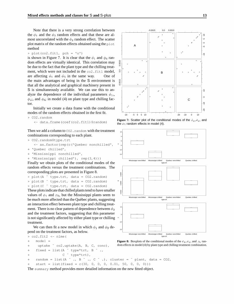
Note that there is a very strong correlation betweenthe �1 and the �3 random effects and that these are al-most uncorrelated with the �2 random effect. The scatterplot matrix of the random effects obtained using the plotmethod> plot(co2.fit1, pch = "o")

is shown in Figure 7. It is clear that the �1 and �3 ran-dom effects are virtually identical. This correlation maybe due to the fact that the plant type and the chilling treat-ment, which were not included in the co2.fit1 model,are affecting �1 and �3 in the same way. One ofthe main advantages of being in the S environment isthat all the analytical and graphical machinery present inS is simultaneously available. We can use this to an-alyze the dependence of the individual parameters �1i,�2i, and �3i in model (4) on plant type and chilling fac-tor.

Initially we create a data frame with the conditionalmodes of the random effects obtained in the first fit.> CO2.random

<- data.frame(coef(co2.fit1)$random)

A

-0.0015 0.0 0.0010

o

oo

o

oo

o o

o

o

o

o

-15

-50

510

o

oo

o

oo

oo

o

o

o

o

-0.0

015

0.0

0.00

10

o

o

o

o

oo

o

o

oo

o

o

B

o

o

o

o

oo

o

o

oo

o

o

-15 -5 0 5 10

o

oo

o

oo

oo

o

o

o

o

o

oo

o

oo

o o

o

o

o

o

-20 -10 0 10

-20

-10

010

C

Figure 7: Scatter plot of the conditional modes of the �1; �2, andthe �3 random effects in model (4).

Then we add a column to CO2.random with the treatmentcombinations corresponding to each plant.> CO2.random$type.trt

<- as.factor(rep(c("Quebec nonchilled",

+ "Quebec chilled",

+ "Mississippi nonchilled",

+ "Mississippi chilled"), rep(3,4)))

Finally we obtain plots of the conditional modes of therandom effects versus the treatment combinations. Thecorresponding plots are presented in Figure 8.> plot(A ˜ type.trt, data = CO2.random)

> plot(B ˜ type.trt, data = CO2.random)

> plot(C ˜ type.trt, data = CO2.random)These plots indicate that chilled plants tend to have smallervalues of �1 and �3, but the Mississippi plants seem tobe much more affected than the Quebec plants, suggestingan interaction effect between plant type and chilling treat-ment. There is no clear pattern of dependence between �2and the treatment factors, suggesting that this parameteris not significantly affected by either plant type or chillingtreatment.

We can then fit a new model in which �1 and �3 de-pend on the treatment factors, as below.> co2.fit2 <- nlme(+ model =

+ uptake ˜ co2.uptake(A, B, C, conc),

-15

-10

-5

0

5

10

A

Mississippi nonchilled Mississippi chilled Quebec nonchilled Quebec chilledtype.trt

-0.0

015

-0.0

005

0.00

05

B


-20

-10

0

10

C


Figure 8: Boxplots of the conditional modes of the �1; �2, and �3 ran-dom effects in model (4) by plant type and chilling treatment combination.

+ fixed = list(A ˜ type*trt, B ˜ .,

+ C ˜ type*trt),

+ random = list(A ˜ ., B ˜ ., C ˜ .), cluster = ˜ plant, data = CO2,

+ start = list(fixed = c(30, 0, 0, 0, 0.01, 50, 0, 0, 0)))

The summary method provides more detailed information on the new fitted object.


> summary(co2.fit2). . .Convergence at iteration: 6Approximate Loglikelihood: -103.5041AIC: 239.0082

Variance/Covariance Components Estimates:Structure: unstructuredParametrization: logcholesky

Standard Deviation(s) of Random Effect(s)A.(Intercept) B C.(Intercept)

2.276278 0.0003200845 5.981132Correlation of Random Effects

A.(Intercept) BB -0.008043761

C.(Intercept) 0.999984502 -0.008100170


Fixed Effects Estimates:Value Approx. Std.Error z ratio(C)

A.(Intercept) 32.452100011 0.7225786330 44.911513A.type -7.909764880 0.7024079993 -11.260927A.trt -4.231594577 0.7009980593 -6.036528

A.type:trt -2.434420834 0.7010132656 -3.472717B 0.009545959 0.0005908485 16.156356

C.(Intercept) 39.936295607 5.6567839253 7.059894C.type -10.469319722 4.2166574898 -2.482848C.trt -7.975396202 4.1963538181 -1.900554

C.type:trt -12.360984497 4.2249903799 -2.925683. . .

The correlation between the �1 and the �3 random effects remains very high, suggesting that the model is probablyoverparametrized and fewer random effects are needed. We will not pursue the model building for the CO2 uptakedata here, since our main goal is to illustrate the use of the methods for the nlme class and not to present a thoroughanalysis of the problem.

To compare co2.fit1 and co2.fit2 we use anova.

> anova(co2.fit1, co2.fit2). . .

Model Df AIC Loglik Test Lik.Ratio P valueco2.fit1 1 10 268.44 -124.22co2.fit2 2 16 239.01 -103.50 1 vs. 2 41.43 2.3824e-07

We see that the inclusion of plant type and chilling treatment in the model caused a substantial increase in the loglike-lihood, indicating that they have a significant effect on �1 and �3.

Diagnostic plots can be obtained with the r option to the plot method

> par(mfrow = c(2,2))> plot(co2.fit2, option = "r", pch = "o")

The corresponding plot is presented in Figure 9. The first plot, observed versus fitted values, indicates that themodel fits the data well — most points lie close to the y = x line. The second plot, residuals versus fitted values, doesnot indicate any departures from the assumptions in the model — no outliers seem to be present and the residuals aresymmetrically scattered around the y = 0 line, with constant spread for different levels of the fitted values.

Predictions are returned by the predict method . For example, to obtain the population predictions of CO2 uptake


o

o

oo

o

oo

o

o

o

ooo

o

o

o

oo oo

o

o

o

o

oo

o

o

o

o

o

o oo

o

o

o

o

o

ooo

o

o

o

o oo

o

o

o

oo o

oo

o

o

ooooo

o

o

o oo

oo

o

o ooooo

o

o ooooo

Fitted Values

Obs

erve

d V

alue

s

10 20 30 40

10

20

30

40

o

o

o

o

o

oo

o

o

o

o

oo

oo

o

o

o

oo

oo

oo

o

o

o

o

o

o

o o

o

o

o

o

o

o

o

oo

o

o

o

oo

o

o

o

o

o

o

o

o

oo

o

o

oo

ooo

oo

ooo

oo

oo

oo

o

oo

o

o

o

oo

o

o

Fitted Values

Res

idua

ls

10 20 30 40

-4

-2

0

2

4

-4

-2

0

2

4

1 2 3 4 5 6 7 8 9 10 11 12

plant

Res

idua

ls

Figure 9: Residuals and fitted values plots.

rate for Quebec and Mississippi plants under chilling and no chilling, at ambient CO2 concentrations of 50; 100; 200,and 500�L=L, we would first define> CO2.new <- data.frame(

+ type = rep(c("Quebec","Mississippi"),

+ c(8, 8)),+ trt = rep(rep(c("chilled","nonchilled"),

+ c(4,4)),2),

+ conc = rep(c(50, 100, 200, 500), 4))

and then use> predict(co2.fit2, CO2.new)

population1 0.05852781

2 11.88120535

. . .

15 28.92219633

16 38.01456512to obtain the predictions.

The predict method can also be used for plotting smoothfitted curves by calculating fitted values at closely spaced con-centrations. Figure 10 presents the individual fitted curves forall twelve plants evaluated at 200 concentrations between 50

Ambient CO2 (uL/L)

CO

2 up

take

rat

e (u

mol

/(m

2 se

c))

200 400 600 800 1000

-10

0

10

20

30

40

50

Mississippi Control

Chilled

Quebec Control

Chilled

Figure 10: Individual fitted curves for the twelve plants in theCO2 uptake data based on the co2.fit2 object.

and 1000 �L=L.


3.3 Structured variance-covariance matrices and random effects blocks

Structured variance-covariance matrices and random effects blocks can also be used for nonlinear mixed-effects mod-els. As in the lme function, the optional arguments re.structure and re.block provide this capability. The usageof these arguments is identical to that in lme, described in section 2.5.

4 Future Developments

The classes and methods described here provide tools for analyzing linear and nonlinear mixed-effects models. As theyare defined within the S environment, all the powerful analytical and graphical machinery present in S is simultaneouslyavailable. The analyses of the dental data, the pixel data, and the CO2 uptake data illustrate some of the availablefeatures, but many other features are available.

The code presented here was developed primarily to handle repeated measures data, i.e. data generated by observinga number of clusters repeatedly under varying experimental conditions. More general mixed effects models (e.g. withdifferent levels of nesting) can be analyzed using the functions described here, but the code will not be computationallyefficient for that purpose.

There are several directions in which the software can be extended to handle more general mixed-effects modelsand/or incorporate other estimation techniques. These include, but are not limited to,� Mixed-effects models in which the variance of the within-subject errors depends on the model function, or some

covariate. The current version of the code assumes constant variance for the within-subject errors.� Mixed-effects models with autocorrelated within-subject errors (Chi and Reinsel, 1989). The current version ofthe code only handles the independent and identically distributed case.� More accurate approximations to the loglikelihood in the nonlinear mixed-effects model (Pinheiro and Bates,1995). These include Laplacian and Gaussian quadrature approximations to the integral that defines the likeli-hood of the data in the nonlinear mixed-effects model. The current version uses an alternating algorithm sug-gested by Lindstrom and Bates (1990).� Profiling methods (Bates and Watts, 1988) for deriving confidence regions on the parameters in the model andassessing the normality of the parameter estimates. These methods are computationally intensive, especially forthe nonlinear mixed-effects model, and efficient programming is needed to make their use feasible.� Update methods for refitting the model when only small changes in the original calling sequence are necessary.These methods are particular useful for model building, when several similar models are fitted sequentially.� Methods for deriving confidence and prediction intervals for predicted values.

We plan to incorporate all these features in future releases of the software to be contributed to the S collection atStatLib.


References

Bates, D. M. and Watts, D. G. (1988). Nonlinear Regression Analysis and Its Applications, Wiley, New York.

Box, G. E. P., Jenkins, G. M. and Reinsel, G. C. (1994). Time Series Analysis: Forecasting and Control, 3rd edn,Holden-Day, San Francisco.

Chambers, J. M. and Hastie, T. J. (eds) (1992). Statistical Models in S, Wadsworth, Belmont, CA.

Chi, E. M. and Reinsel, G. C. (1989). Models for longitudinal data with random effects and AR(1) errors, Journal ofthe American Statistical Association 84: 452–459.

Laird, N., Lange, N. and Stram, D. (1987). Maximum likelihood computations with repeated measures: Applicationof the EM algorithm, Journal of the American Statistical Association 82: 97–105.

Laird, N. M. and Ware, J. H. (1982). Random-effects models for longitudinal data, Biometrics 38: 963–974.

Lindstrom, M. J. and Bates, D. M. (1990). Nonlinear mixed effects models for repeated measures data, Biometrics46: 673–687.

Pinheiro, J. C. (1994). Topics in Mixed Effects Models, PhD thesis, University of Wisconsin–Madison.

Pinheiro, J. C. and Bates, D. M. (1995). Approximations to the loglikelihood function in the nonlinear mixed effectsmodel, Journal of Computational and Graphical Statistics. To appear.

Potthoff, R. F. and Roy, S. N. (1964). A generalized multivariate analysis of variance model useful especially for growthcurve problems, Biometrika 51: 313–326.

Potvin, C. and Lechowicz, M. J. (1990). The statistical analysis of ecophysiological response curves obtained fromexperiments involving repeated measures, Ecology 71: 1389–1400.


Appendix A

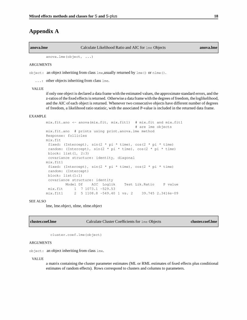
anova.lme Calculate Likelihood Ratio and AIC for lme Objects anova.lme

anova.lme(object, ...)

ARGUMENTS

object: an object inheriting from class lme,usually returned by lme() or nlme().

...: other objects inheriting from class lme.

VALUEif only one object is declared a data frame with the estimated values, the approximate standard errors, and thez-ratios of the fixed effects is returned. Otherwise a data frame with the degrees of freedom, the loglikelihood,and the AIC of each object is returned. Whenever two consecutive objects have different number of degreesof freedom, a likelihood ratio statistic, with the associated P-value is included in the returned data frame.

EXAMPLE

mix.fit.ano <- anova(mix.fit, mix.fit1) # mix.fit and mix.fit1# are lme objects

mix.fit.ano # prints using print.anova.lme methodResponse: folliclesmix.fitfixed: (Intercept), sin(2 * pi * time), cos(2 * pi * time)random: (Intercept), sin(2 * pi * time), cos(2 * pi * time)block: list(1, 2:3)covariance structure: identity, diagonalmix.fit1fixed: (Intercept), sin(2 * pi * time), cos(2 * pi * time)random: (Intercept)block: list(1:1)covariance structure: identity

Model Df AIC Loglik Test Lik.Ratio P valuemix.fit 1 7 1073.1 -529.53mix.fit1 2 5 1108.8 -549.40 1 vs. 2 39.745 2.3416e-09

SEE ALSOlme, lme.object, nlme, nlme.object

cluster.coef.lme Calculate Cluster Coefficients for lme Objects cluster.coef.lme

cluster.coef.lme(object)

ARGUMENTS

object: an object inheriting from class lme.

VALUEa matrix containing the cluster parameter estimates (ML or RML estimates of fixed effects plus conditionalestimates of random effects). Rows correspond to clusters and columns to parameters.


EXAMPLE

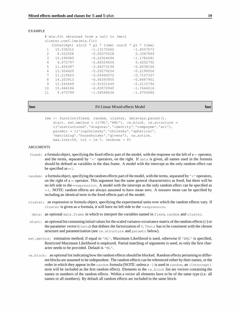
# mix.fit obtained from a call to lme()cluster.coef.lme(mix.fit)

(Intercept) sin(2 * pi * time) cos(2 * pi * time)1 15.536312 -1.13172662 -1.45570732 8.032558 -0.05075528 0.33478993 15.296980 -4.22924696 -1.17820814 6.672797 -2.86559654 0.42527925 11.456387 -3.66373194 -0.60381666 13.954620 -5.29279204 -0.21900567 11.219623 -3.05460072 -0.71073378 14.203913 -6.68393955 -0.84879619 12.545649 -2.91031449 -2.211579410 15.664186 -4.83072940 -1.764421611 9.475799 -1.56596434 -1.4705484

lme Fit Linear Mixed-effects Model lme

lme <- function(fixed, random, cluster, data=sys.parent(),start, est.method = c("ML","RML"), re.block, re.structure =c("unstructured","diagonal","identity","compsymm","ar1"),paramtr = c("logcholesky","cholesky","spherical","matrixlog","householder","givens"), na.action,max.iter=50, tol = 1e-7, verbose = F)

ARGUMENTS

fixed: a formula object, specifying the fixed effects part of the model, with the response on the left of a � operator,and the terms, separated by "+" operators, on the right. If data is given, all names used in the formulashould be defined as variables in the data frame. A model with the intercept as the only random effect canbe specified as �1.

random: a formula object, specifying the random effects part of the model, with the terms, separated by "+" operators,on the right of a � operator. This argument has the same general characteristics as fixed, but there will beno left side to the �expression. A model with the intercept as the only random effect can be specified as�1. NOTE: random effects are always assumed to have mean zero. A nonzero mean can be specified byincluding an identical term in the fixed effects part of the model.

cluster: an expression or formula object, specifying the experimental units over which the random effects vary. Ifcluster is given as a formula, it will have no left side to the �expression.

data: an optional data.frame in which to interpret the variables named in fixed, random and cluster.

start: an optional list containing initial values for the scaled variance-covariance matrix of the random effects (D) orthe parameter vector (theta) that defines the factorization of D. Theta has to be consistent with the chosenstructure and parametrization (see re.structure and paramtr below).

est.method: estimation method; if equal to "ML", Maximum Likelihood is used, otherwise if "RML" is specified,Restricted Maximum Likelihood is employed. Partial matching of arguments is used, so only the first char-acter needs to be provided. Default is "ML".

re.block: an optional list indicating how the random effects should be blocked. Random effects pertaining to differ-ent blocks are assumed to be independent. The random effects can be referenced either by their names, or theorder in which they appear in the random formula (NOTE: unless a -1 is used in random, an (Intercept)term will be included as the first random effect). Elements in the re.block list are vectors containing thenames or numbers of the random effects. Within a vector all elements have to be of the same type (i.e. allnames or all numbers). By default all random effects are included in the same block.


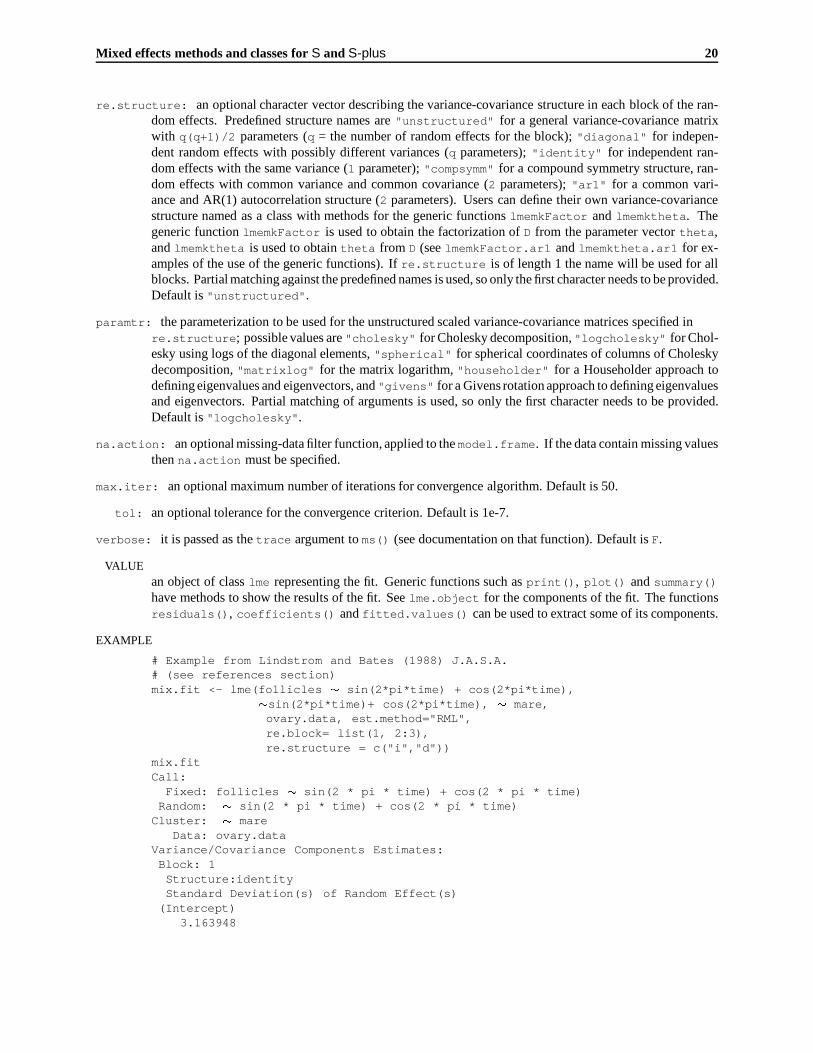
re.structure: an optional character vector describing the variance-covariance structure in each block of the ran-dom effects. Predefined structure names are "unstructured" for a general variance-covariance matrixwith q(q+1)/2 parameters (q = the number of random effects for the block); "diagonal" for indepen-dent random effects with possibly different variances (q parameters); "identity" for independent ran-dom effects with the same variance (1 parameter); "compsymm" for a compound symmetry structure, ran-dom effects with common variance and common covariance (2 parameters); "ar1" for a common vari-ance and AR(1) autocorrelation structure (2 parameters). Users can define their own variance-covariancestructure named as a class with methods for the generic functions lmemkFactor and lmemktheta. Thegeneric function lmemkFactor is used to obtain the factorization of D from the parameter vector theta,and lmemktheta is used to obtain theta from D (see lmemkFactor.ar1 and lmemktheta.ar1 for ex-amples of the use of the generic functions). If re.structure is of length 1 the name will be used for allblocks. Partial matching against the predefined names is used, so only the first character needs to be provided.Default is "unstructured".

paramtr: the parameterization to be used for the unstructured scaled variance-covariance matrices specified inre.structure; possible values are "cholesky" for Cholesky decomposition, "logcholesky" for Chol-esky using logs of the diagonal elements, "spherical" for spherical coordinates of columns of Choleskydecomposition, "matrixlog" for the matrix logarithm, "householder" for a Householder approach todefining eigenvalues and eigenvectors, and "givens" for a Givens rotation approach to defining eigenvaluesand eigenvectors. Partial matching of arguments is used, so only the first character needs to be provided.Default is "logcholesky".

na.action: an optional missing-data filter function, applied to the model.frame. If the data contain missing valuesthen na.action must be specified.

max.iter: an optional maximum number of iterations for convergence algorithm. Default is 50.

tol: an optional tolerance for the convergence criterion. Default is 1e-7.

verbose: it is passed as the trace argument to ms() (see documentation on that function). Default is F.

VALUEan object of class lme representing the fit. Generic functions such as print(), plot() and summary()

have methods to show the results of the fit. See lme.object for the components of the fit. The functionsresiduals(), coefficients() and fitted.values() can be used to extract some of its components.

EXAMPLE

# Example from Lindstrom and Bates (1988) J.A.S.A.# (see references section)mix.fit <- lme(follicles � sin(2*pi*time) + cos(2*pi*time),�sin(2*pi*time)+ cos(2*pi*time), � mare,

ovary.data, est.method="RML",re.block= list(1, 2:3),re.structure = c("i","d"))

mix.fitCall:

Fixed: follicles � sin(2 * pi * time) + cos(2 * pi * time)Random: � sin(2 * pi * time) + cos(2 * pi * time)Cluster: � mare

Data: ovary.dataVariance/Covariance Components Estimates:Block: 1Structure:identityStandard Deviation(s) of Random Effect(s)

(Intercept)3.163948


Block: 2Structure:diagonalStandard Deviation(s) of Random Effect(s)

sin(2 * pi * time) cos(2 * pi * time)2.089664 1.054145


Fixed Effects Estimates:(Intercept) sin(2 * pi * time) cos(2 * pi * time)

12.18717 -3.298127 -0.882068Number of Observations: 308Number of Clusters: 11

REFERENCESThe computational methods are described in Lindstrom,M.J. and Bates, D.M. (1988) ”Newton-Raphson andEM Algorithms for Linear Mixed-Effects Models for Repeated-Measures Data”, Journal of the AmericanStatistical Association, 83, 1014-1022. The general method is described in Laird, N.M. and Ware, J.H.(1982) ”Random-Effects Models for Longitudinal Data”, Biometrics, 38, 963-974.

lme.object Linear Mixed-effects Model Object lme.object

This class of objects is returned from the lme() function to represent a fitted linear mixed-effects model.Objects of this class have methods for the generic functions anova(), coef(), cluster.coef(), fitted(), plot(), predict(), print(), residuals(), and summary().

COMPONENTSThe following components must be included in a legitimate lme object. The residuals, fitted values andcoefficients can be extracted by the generic functions of the same name, or by the "$" operator.

coefficients: a list with two components, fixed and random, where the first is a vector containing the estimatedcoefficients for the fixed effects - the names of the coefficients are the same as those in the fixed formula ofthe call to lme(), and the second is a matrix containing the estimated coefficients for the random effects.The columns refer to the parameters in the random formula, and the rows to the cluster levels; the namesof the coefficients are the same as in the random formula (columns) and the cluster levels (rows).

fitted.values: a list containing the population and cluster fitted values. The population fitted values are evaluatedat the converged estimates of the fixed effects and the mean of the random effects (i.e. the random effectsare set to zero). The cluster fitted values are evaluated at the converged estimates of the fixed effects and theconditional estimates of the random effects.

residuals: a list containing the population and cluster residuals from the fit. The population residuals are the ob-served values minus the population fitted values and the cluster residuals are the observed values minus thecluster fitted values.

var.ran: Random effects variance-covariance-correlation matrix estimate. The variances estimates for the randomeffects are displayed on the main diagonal, covariances above the diagonal and correlations below the diag-onal.

var.fix: the conditional variance-covariance matrix of the fixed effects (i.e. the variance-covariance matrix of thefixed effects given the random effects).

sigma: estimate of the cluster residual standard deviation.

call: a list containing an image of the lme() call.

cluster: a vector containing the clusters levels.


nobs,nclus: the number of observations (nobs) and clusters (nclus) used in the fit.

loglik: the loglikelihood value at convergence.

est.method: estimation method used in the fit, either "ML" or "RML".

fixed,random: formulas representing the fixed and random components of the model.

niter: number of iterations used in iterative algorithm.

re.block,re.structure: the blocking and covariance structures used for the random effects.

paramtr: the parametrization used for the unstructured variance-covariance matrices of the blocks of random effects.

sizetheta: length of the parameter vector theta used to obtain the scaled variance-covariance matrix of the randomeffects D.

SEE ALSOlme

nlme Fit a Nonlinear Mixed-effects Model nlme

nlme <- function(model, fixed, random, cluster,data = sys.parent(), start, est.method = c("ML","RML"),re.block, re.structure = c("unstructured", "diagonal","identity", "compsymm", "ar1"), paramtr = c("logcholesky","cholesky","spherical","matrixlog", "householder","givens"), control, na.action, na.pattern, verbose = F)

ARGUMENTS

model: a nonlinear model formula with the response on the left of a � operator, and an expression involving pa-rameters and covariates on the right. If data is given, all names used in the formula should be defined asparameters or variables in the data frame.

fixed: a list of formulas of the parameter fixed effects. Usually there will be a fixed effects formula for each pa-rameter. A . on the right hand side of a formula indicates a single fixed effect for that parameter, a formulais evaluated as a linear formula in the frame (data).

random: a list of formulas of the parameter random effects. There need not be a random effect formula for eachparameter. A . on the right hand side of a formula indicates a single random effect for that parameter,aformula is evaluated as a linear formula in the frame (data). NOTE: random effects are always assumed tohave mean zero. A nonzero mean can be specified by including an identical term in the fixed effects part ofthe model.

cluster: an expression or formula object, specifying the experimental units over which the random effects vary. Ifcluster is given as a formula, it will have no left side to the �expression.

data: an optional data.frame in which to interpret the variables named in fixed, random and cluster andcovariates referenced in the first two.

start: a list of initial estimates for the parameters. The fixed component is required. The order of initial esti-mates in that component corresponds to the order in the fixed argument. Optional components are random,D (scaled variance-covariance matrix of the random effects), and theta (the factorized form of the scaledvariance-covariance matrix of the random effects). If present, the random component should be a matrixwith as many rows as there are random effects and as many columns as there are clusters. Theta has to beconsistent with the chosen structure and parametrization (see re.structure and paramtr below).


est.method: estimation method; if equal to "ML", Maximum Likelihood is used, otherwise if "RML" is specified,Residual Maximum Likelihood is employed. Partial matching of arguments is used, so only the first characterneeds to be provided. Default is "ML".

re.block: an optional list indicating how the random effects should be blocked. Random effects pertaining to differ-ent blocks are assumed to be independent. The random effects can be referenced either by their names, or theorder in which they appear in the random formula (NOTE: unless a -1 is used in random, an (Intercept)term will be included as the first random effect). Elements in the re.block list are vectors containing thenames or numbers of the random effects. Within a vector all elements have to be of the same type (i.e. allnames or all numbers). By default all random effects are included in the same block.

re.structure: an optional character vector describing the variance-covariance structure in each block of the ran-dom effects. Predefined structure names are "unstructured" for a general variance-covariance matrixwith q(q+1)/2 parameters (q = the number of random effects for the block); "diagonal" for indepen-dent random effects with possibly different variances (q parameters); "identity" for independent ran-dom effects with the same variance (1 parameter); "compsymm" for a compound symmetry structure, ran-dom effects with common variance and common covariance (2 parameters); "ar1" for a common vari-ance and AR(1) autocorrelation structure (2 parameters). Users can define their own variance-covariancestructure named as a class with methods for the generic functions lmemkFactor and lmemktheta. Thegeneric function lmemkFactor is used to obtain the factorization of D from the parameter vector theta,and lmemktheta is used to obtain theta from D (see lmemkFactor.ar1 and lmemktheta.ar1 for ex-amples of the use of the generic functions). If re.structure is of length 1 the name will be used for allblocks. Partial matching against the predefined names is used, so only the first character needs to be provided.Default is "unstructured".

paramtr: the parameterization to be used for the unstructured scaled variance-covariance matrices specified inre.structure; possible values are "cholesky" for Cholesky decomposition, "logcholesky" for Chol-esky using logs of the diagonal elements, "spherical" for spherical coordinates of columns of Choleskydecomposition, "matrixlog" for the matrix logarithm, "householder" for a Householder approach todefining eigenvalues and eigenvectors, and "givens" for a Givens rotation approach to defining eigenvaluesand eigenvectors. Partial matching of arguments is used, so only the first character needs to be provided.Default is "logcholesky".

control: an optional list of control values for the nonlinear estimation algorithm.

na.action: an optional missing-data filter function, applied to the model.frame. If the data contain missing valuesthen na.action must be specified.

na.pattern: an optional expression or formula object, specifying which returned values are to be regarded as miss-ing.

verbose: if T (TRUE) information on the evolution of the iterative algorithm (number of iterations, convergence cri-terion, etc.) will be printed. Default is F.

VALUEan object of class nlme representing the fit. Generic functions such as print(), plot(), predict, andsummary() have methods to show the results of the fit. See nlme.object for the components of the fit.The functions residuals(), coefficients() and fitted.values() can be used to extract some of itscomponents.

SEE ALSOnlme.control


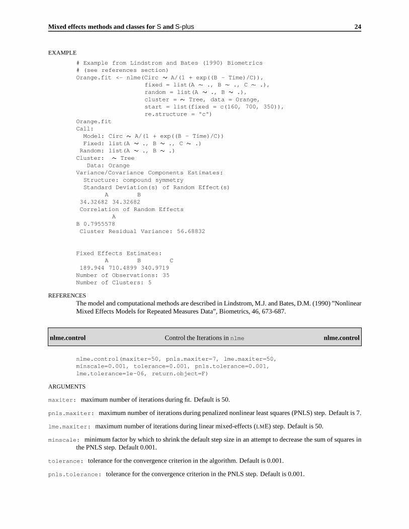
EXAMPLE

# Example from Lindstrom and Bates (1990) Biometrics# (see references section)Orange.fit <- nlme(Circ � A/(1 + exp((B - Time)/C)),

fixed = list(A � ., B � ., C � .),random = list(A � ., B � .),cluster = � Tree, data = Orange,start = list(fixed = c(160, 700, 350)),re.structure = "c")

Orange.fitCall:

Model: Circ � A/(1 + exp((B - Time)/C))Fixed: list(A � ., B � ., C � .)

Random: list(A � ., B � .)Cluster: � Tree

Data: OrangeVariance/Covariance Components Estimates:

Structure: compound symmetryStandard Deviation(s) of Random Effect(s)

A B34.32682 34.32682Correlation of Random Effects

AB 0.7955578Cluster Residual Variance: 56.68832

Fixed Effects Estimates:A B C

189.944 710.4899 340.9719Number of Observations: 35Number of Clusters: 5

REFERENCESThe model and computational methods are described in Lindstrom, M.J. and Bates, D.M. (1990) ”NonlinearMixed Effects Models for Repeated Measures Data”, Biometrics, 46, 673-687.

nlme.control Control the Iterations in nlme nlme.control

nlme.control(maxiter=50, pnls.maxiter=7, lme.maxiter=50,minscale=0.001, tolerance=0.001, pnls.tolerance=0.001,lme.tolerance=1e-06, return.object=F)

ARGUMENTS

maxiter: maximum number of iterations during fit. Default is 50.

pnls.maxiter: maximum number of iterations during penalized nonlinear least squares (PNLS) step. Default is 7.

lme.maxiter: maximum number of iterations during linear mixed-effects (LME) step. Default is 50.

minscale: minimum factor by which to shrink the default step size in an attempt to decrease the sum of squares inthe PNLS step. Default 0.001.

tolerance: tolerance for the convergence criterion in the algorithm. Default is 0.001.

pnls.tolerance: tolerance for the convergence criterion in the PNLS step. Default is 0.001.


lme.tolerance: tolerance for the convergence criterion in the LME step, passed as the rel.tolerance argumentto ms() (see documentation on that function). Default is 1e-6.

return.object: if T (TRUE) the fitted object is returned by nlme() when the maximum number of iterations isattained without convergence. Default is F.

VALUEa list containing components for each of the possible arguments, either the value supplied by the user or thedefault.

EXAMPLE

# increase the maximum number of iterations in the PNLS step# and return the object when maximum number of iterations is# attained without convergencenlme.control(pnls.maxiter = 20, return.object = T)

nlme.object Nonlinear Mixed-effects Model Object nlme.object

This class of objects is returned from thenlme() function to represent a fitted nonlinearmixed-effects model.Objects of this class have methods for the generic functions anova(), coef(), cluster.coef(), fit-ted(), plot(), predict(), print(), residuals(), and summary(). Objects from this class inheritfrom the lme class.

COMPONENTSThe following components must be included in a legitimate nlme object. The residuals, fitted values andcoefficients can be extracted by the generic functions of the same name, or by the "$" operator.

coefficients: a list with two components, fixed and random, where the first is a vector containing the estimatedcoefficients for the fixed effects and the second is a matrix containing the estimated coefficients for the ran-dom effects. The columns refer to the parameters in the random formula, and the rows to the cluster

levels; the names of the coefficients are the same as those in the fixed or random formulas when just a . isused on the right hand side, or the original name with the covariate name appended to it (i.e. name.covariate)otherwise.

fitted.values: a list containing the population and cluster fitted values. The population fitted values are evaluatedat the converged estimates of the fixed effects and the mean of the random effects (i.e. the random effectsare set to zero). The cluster fitted values are evaluated at the converged estimates of the fixed effects and theconditional estimates of the random effects.

residuals: a list containing the population and cluster residuals from the fit. The population residuals are the ob-served values minus the population fitted values and the cluster residuals are the observed values minus thecluster fitted values.

var.ran: Random effects variance-covariance-correlation matrix estimate. The variances estimates for the randomeffects are displayed on the main diagonal, covariances above the diagonal and correlations below the diag-onal.

var.fix: the conditional variance-covariance matrix of the fixed effects (i.e. the variance-covariance matrix of thefixed effects given the random effects).

sigma: estimate of the cluster residual standard deviation.

loglik: the approximate log likelihood at convergence.

cluster: a vector containing the clusters labels.


call: a list containing an image of the nlme() call.

nobs,nclus: the number of observations (nobs) and clusters (nclus) used in the fit.

est.method: estimation method used in the fit, either "ML" or "RML".

niter: number of iterations used in iterative algorithm.

re.block,re.structure: the blocking and covariance structures used for the random effects.

paramtr: the parametrization used for the unstructured variance-covariance matrices of the blocks of random effects.

sizetheta: length of the parameter vector theta used to obtain the scaled variance-covariance matrix of the randomeffects D.

criterion: a vector containing the values of the convergence criteria for the fixed and random effects and the factorof the scaled covariance matrix of the random effects.

SEE ALSOnlme

plot.lme Plot Components of a lme Object plot.lme

plot.lme(object, option = c("c","r","s"), resid.type = c("c","p"),which = 1:3, ...)

ARGUMENTS


option: if "r" or "s", diagnostic plots for the fitted values and the raw ("r") or standardized ("s") residuals arereturned; otherwise, if option is set to "c", the function returns plots for the random effects coefficients.Default is "c".

resid.type: if "c", the cluster residuals are used, otherwise, if "p", the population residuals are used. Default is"c". See the help file for lme.object for definitions of cluster and population residuals and fitted values.

which: an optional integer vector specifying which plots should be generated when option is set to "r" or "s".Available options include observed versus fitted values (1), residuals versus fitted values (2), and residualsby cluster (3). Default is 1:3 (all plots generated).

...: optional plot settings arguments.

VALUEFor either the raw residuals or the standardized residuals, three diagnostic plots are returned : response vs.fitted.values, residuals vs. fitted.values and residuals vs. cluster. For the random effectscoefficients, if just one coefficient is present in the model, the normal plot of the coefficients is returned; if twocoefficients are used, a scatter plot is returned; otherwise a scatter plot matrix with all pairwise combinationsof the random coefficients is returned.

EXAMPLE

> plot.lme(mix.fit)> plot.lme(mix.fit,"s","p")


predict.lme Make Predictions from a Fitted lme Object predict.lme

predict.lme(object, cluster, data, na.action)

ARGUMENTS


cluster: an optional expression or formula object, specifying the cluster associated with each observation for whichthe prediction is required; if cluster is given as a formula, there shouldbe no left hand side to the�expres-sion. If cluster is not specified only the population predictions are calculated. Missing values are al-lowed for cluster, in which case only the population prediction is calculated and the cluster predic-tion is set to NA. See the help file for lme.object or nlme.object for definitions of cluster and populationresiduals and fitted values.

data: a data.frame containing the values at which predictions are required. Only those predictors, referred to inthe right side of the fixed and random formulas in object, need be present by name in data.

na.action: an optional missing-data filter function, applied to the model.frame. If the data contain missing valuesthe na.action must be specified.

VALUEa data.frame containing either two components : cluster - the clusters associated with each predictionand fit - a data.frame with columns population - the predictions based solely on the fixed effects es-timates and cluster - the predictions using both the fixed effects estimates and the posterior modes of therandom effects, when cluster is specified or only the population column, otherwise.

EXAMPLE

# defining the new data frame for predictionsovary.new <-data.frame(time = c(0, 0.25, 0.5, 0.75, 1),mare = c(1, 1, 2, 2, 3))predict.lme(mix.fit,�mare,ovary.new)

cluster fit.cluster fit.population1 1 14.080605 11.3050982 1 14.404586 8.8890393 2 7.697768 13.0692344 2 8.083313 15.4852935 3 14.118772 11.305098

SEE ALSOlme, lme.object

print.lme Use print() on a lme Object print.lme

print.lme(x, ...)

This function is a method for the generic function print() for class "lme". It can be invoked by callingprint(x) for an object x of the appropriate class, or directly by calling print.lme(), regardless of theclass of the object. See print or print.default for the general behavior of this function and for theinterpretation of x.


summary.lme Summarize a lme Object summary.lme

summary.lme(object, re = T)

ARGUMENTS

object: an object inheriting from class lme().

re: if T (TRUE), the conditional modes of the random effects are included in the returned object. Default is T.

VALUEa structure with the appropriate summary information. The components includecorrelations, fixed.ta-ble, random.table, call, nobs, nclus, loglik, AIC, niter, sigma, est.method, paramtr, , resid-uals, and resid.type. The AIC component gives the Akaike Information Criteria, defined as -2*loglike-lihood + 2*(number of parameters in the model). The object returned is of class summary.lme. A print

method is available for this class. NOTE : the z ratio in the fixed.table component is included simply as aguideline for screening variables. The recommended approach for deleting variables from the model is torefit the reduced model and test the significance of the reduction in the loglikelihood, when compared to theoriginal fit.

EXAMPLE

mix.fit.summ <- summary(mix.fit) # mix.fit is a lme objectmix.fit.summ # prints using print.summary.lme methodCall:

Fixed: follicles � sin(2 * pi * time) + cos(2 * pi * time)Random: � sin(2 * pi * time) + cos(2 * pi * time)Cluster: � mare

Data: ovary.dataEstimation Method: RMLConvergence at iteration: 7Restricted Loglikelihood: -529.5315Restricted AIC: 1073.063Variance/Covariance Components Estimates:Block: 1Structure:identityStandard Deviation(s) of Random Effect(s)

(Intercept)3.163948

Block: 2Structure:diagonalStandard Deviation(s) of Random Effect(s)

sin(2 * pi * time) cos(2 * pi * time)2.089664 1.054145

Cluster Residual Variance: 9.12222Fixed Effects Estimates:

Value Approx. Std.Error z ratio(C)(Intercept) 12.187166 0.9707129 12.554862

sin(2 * pi * time) -3.298127 0.6805604 -4.846193cos(2 * pi * time) -0.882068 0.3992836 -2.209127Conditional Correlations of Fixed Effects Estimates

(Intercept) sin(2 * pi * time)sin(2 * pi * time) -4.050516e-17cos(2 * pi * time) -3.125134e-02 4.115554e-17


Random Effects (Conditional Estimates):(Intercept) sin(2 * pi * time) cos(2 * pi * time)

1 3.3491465 2.1664005 -0.573639342 -4.1546083 3.2473718 1.216857893 3.1098142 -0.9311199 -0.296140184 -5.5143693 0.4325305 1.307347125 -0.7307790 -0.3656049 0.278251376 1.7674541 -1.9946650 0.663062397 -0.9675429 0.2435264 0.171334298 2.0167471 -3.3858125 0.033271859 0.3584834 0.3878126 -1.3295114110 3.4770206 -1.5326023 -0.8823536011 -2.7113664 1.7321627 -0.58848038

Standardized Cluster Residuals:Min Q1 Med Q3 Max

-2.688067 -0.5996717 -0.03194583 0.5487485 4.267131Number of Observations: 308Number of Clusters: 11

SEE ALSOlme, lme.object, print.lme

mixed effects models methods and classes for s and splus ...sun.cwru.edu/~jiayang/nlme.pdf ·...

Documents