mit 2.852 manufacturing systems analysis lectures … · flow line analysis difficulties ......
TRANSCRIPT

MIT 2.852
Manufacturing Systems Analysis
Lectures 6–9: Flow Lines
Models That Can Be Analyzed Exactly
Stanley B. Gershwin
http://web.mit.edu/manuf-sys
Massachusetts Institute of Technology
Spring, 2010
2.852 Manufacturing Systems Analysis 1/165 ©2010 Stanley B. Gershwin. Copyright c

Models
◮ The purpose of an engineering or scientific model is to make predictions.
◮ Kinds of models: ◮ Mathematical: aggregated behavior is described by equations.
Predictions are made by solving the equations. ◮ Simulation: detailed behavior is described. Predictions are made by
reproducting behavior.
◮ Models are simplifications of reality. ◮ Models that are too simple make poor predictions because they leave
out important features. ◮ Models that are too complex make poor predictions because they are
difficult to analyze or are time-consuming to use, because they require more data, or because they have errors.
2.852 Manufacturing Systems Analysis 2/165 Copyright c©2010 Stanley B. Gershwin.
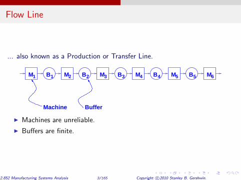
Flow Line
... also known as a Production or Transfer Line.
Machine Buffer
M1 M2 M3 4 M5 M6MB1 B2 B3 B4 B5
◮ Machines are unreliable.
◮ Buffers are finite.
2.852 Manufacturing Systems Analysis 3/165 Copyright c©2010 Stanley B. Gershwin.

Flow Line Motivation
◮ Economic importance.
◮ Relative simplicity for analysis and for intuition.
2.852 Manufacturing Systems Analysis 4/165 Copyright c©2010 Stanley B. Gershwin.
Flow Line
Buffers and Inventory
◮ Buffers are for mitigating asynchronization (ie, they are shock absorbers).
◮ Buffer space and inventory are expensive.
2.852 Manufacturing Systems Analysis 5/165 Copyright c©2010 Stanley B. Gershwin.

Flow Line Analysis Difficulties
◮ Complex behavior.
◮ Analytical solution available only for limited systems.
◮ Exact numerical solution feasible only for systems with a small number of buffers.
◮ Simulation may be too slow for optimization.
2.852 Manufacturing Systems Analysis 6/165 Copyright c©2010 Stanley B. Gershwin.
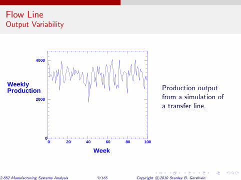
Flow Line Output Variability
Week
Weekly Production
0 20 40 60 80 100 0
2000
4000
Production output from a simulation of a transfer line.
2.852 Manufacturing Systems Analysis 7/165 Copyright c©2010 Stanley B. Gershwin.

Flow Line Usual General Assumptions
◮ Unlimited repair personnel.
◮ Uncorrelated failures.
◮ Perfect yield.
◮ The first machine is never starved and the last is never blocked.
◮ Blocking before service.
◮ Operation dependent failures.
2.852 Manufacturing Systems Analysis 8/165 Copyright c©2010 Stanley B. Gershwin.

Single Reliable Machine
◮ If the machine is perfectly reliable, and its average operation time is τ , then its maximum production rate is 1/τ .
◮ Note:
◮ Sometimes cycle time is used instead of operation time , but BEWARE: cycle time has two meanings!
◮ The other meaning is the time a part spends in a system. If the system is a single, reliable machine, the two meanings are the same.
2.852 Manufacturing Systems Analysis 9/165 Copyright c©2010 Stanley B. Gershwin.

Single Unreliable Machine ODFs
◮ Operation-Dependent Failures
◮ A machine can only fail while it is working. ◮ IMPORTANT! MTTF must be measured in working time! ◮ This is the usual assumption.
◮ Note: MTBF = MTTF + MTTR
2.852 Manufacturing Systems Analysis 10/165 Copyright c©2010 Stanley B. Gershwin.
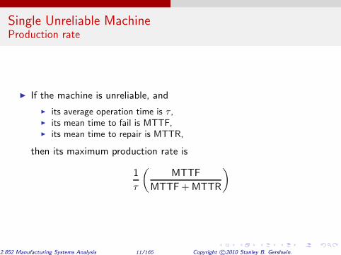
Single Unreliable Machine Production rate
◮ If the machine is unreliable, and
◮ its average operation time is τ , ◮ its mean time to fail is MTTF, ◮ its mean time to repair is MTTR,
then its maximum production rate is
1
τ
( MTTF
MTTF + MTTR
)
2.852 Manufacturing Systems Analysis 11/165 Copyright c©2010 Stanley B. Gershwin.

Single Unreliable Machine Production rate
Proof
Machine DOWNMachine UP
◮ Average production rate, while machine is up, is 1/τ .
◮ Average duration of an up period is MTTF.
◮ Average production during an up period is MTTF/τ .
◮ Average duration of up-down period: MTTF + MTTR.
◮ Average production during up-down period: MTTF/τ .
◮ Therefore, average production rate is
(MTTF/τ)/(MTTF + MTTR).
2.852 Manufacturing Systems Analysis 12/165 Copyright c©2010 Stanley B. Gershwin.
Single Unreliable Machine Geometric Up- and Down-Times
◮ Assumptions: Operation time is constant (τ). Failure and repair times are geometrically distributed.
◮ Let p be the probability that a machine fails during any given operation. Then p = τ/MTTF.
2.852 Manufacturing Systems Analysis 13/165 Copyright c©2010 Stanley B. Gershwin.

Single Unreliable Machine
◮ Let r be the probability that M gets repaired in during any operation time when it is down. Then r = τ/MTTR.
◮ Then the average production rate of M is
1
τ
( r
r + p
)
.
◮ (Sometimes we forget to say “average.”)
2.852 Manufacturing Systems Analysis 14/165 Copyright c©2010 Stanley B. Gershwin.
Single Unreliable Machine Production Rates
◮ So far, the machine really has three production rates: ◮ 1/τ when it is up (short-term capacity) , ◮ 0 when it is down (short-term capacity) , ◮ (1/τ)(r/(r + p)) on the average (long-term capacity) .
2.852 Manufacturing Systems Analysis 15/165 Copyright c©2010 Stanley B. Gershwin.

Infinite-Buffer Line
M B1 1 M B2 2 B3 3 M B4 4 M B5 5 M6M
Assumptions:
◮ A machine is not idle if it is not starved.
◮ The first machine is never starved.
2.852 Manufacturing Systems Analysis 16/165 Copyright c©2010 Stanley B. Gershwin.

Infinite-Buffer Line
M B1 1 M B2 2 B3 3 M B4 4 M B5 5 M6M
◮ The production rate of the line is the production rate of the slowest machine in the line — called the bottleneck .
◮ Slowest means least average production rate, where average production rate is calculated from one of the previous formulas.
2.852 Manufacturing Systems Analysis 17/165 Copyright c©2010 Stanley B. Gershwin.

Infinite-Buffer Line
M B1 1 M B2 2 B3 3 M B4 4 M B5 5 M6M
◮ Production rate is therefore
P = min i
1
τi
( MTTFi
MTTFi + MTTRi
)
◮ and Mi is the bottleneck.
2.852 Manufacturing Systems Analysis 18/165 Copyright c©2010 Stanley B. Gershwin.
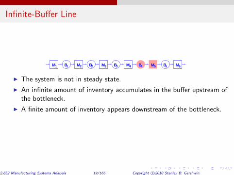
Infinite-Buffer Line
M B1 1 M B2 2 B3 3 M4 4 M B5 5 M6M B
◮ The system is not in steady state.
◮ An infinite amount of inventory accumulates in the buffer upstream of the bottleneck.
◮ A finite amount of inventory appears downstream of the bottleneck.
2.852 Manufacturing Systems Analysis 19/165 Copyright c©2010 Stanley B. Gershwin.
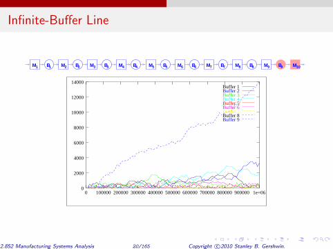
Infinite-Buffer Line
M8 8 M B9 9 M10BM B5 5 M B6 6 B7 7MM B3 3 B4 4MM B2 2M B1 1
0
2000
4000
6000
8000
10000
12000
14000
0 100000 200000 300000 400000 500000 600000 700000 800000 900000 1e+06
Buffer 1 Buffer 2 Buffer 3 Buffer 4 Buffer 5 Buffer 6 Buffer 7 Buffer 8 Buffer 9
2.852 Manufacturing Systems Analysis 20/165 Copyright c©2010 Stanley B. Gershwin.

Infinite-Buffer Line
M8 8 M B9 9 M10BM B5 5 M B6 6 B7 7MM B3 3 B4 4MM B2 2M B1 1
◮ The second bottleneck is the slowest machine upstream of the bottleneck. An infinite amount of inventory accumulates just upstream of it.
◮ A finite amount of inventory appears between the second bottleneck and the machine upstream of the first bottleneck.
◮ Et cetera.
2.852 Manufacturing Systems Analysis 21/165 Copyright c©2010 Stanley B. Gershwin.

Infinite-Buffer Line
M8 8 M B9 9 M10BM B5 5 M B6 6 B7 7MM B3 3 B4 4MM B2 2M B1 1
0
2000
4000
6000
8000
10000
12000
0 100000 200000 300000 400000 500000 600000 700000 800000 900000 1e+06
Buffer 1 Buffer 2 Buffer 3 Buffer 4 Buffer 5 Buffer 6 Buffer 7 Buffer 8 Buffer 9
A 10-machine line with bottlenecks at Machines 5 and 10.
2.852 Manufacturing Systems Analysis 22/165 Copyright c©2010 Stanley B. Gershwin.

Infinite-Buffer Line
M8 8 M B9 9 M10BM B5 5 M B6 6 B7 7MM B3 3 B4 4MM B2 2M B1 1
0
2000
4000
6000
8000
10000
12000
0 100000 200000 300000 400000 500000 600000 700000 800000 900000 1e+06
Buffer 4 Buffer 9
Question:
◮ What are the slopes (roughly!) of the two indicated graphs?
2.852 Manufacturing Systems Analysis 23/165 Copyright c©2010 Stanley B. Gershwin.
Infinite-Buffer Line
Questions:
◮ If we want to increase production rate, which machine should we improve?
◮ What would happen to production rate if we improved any other machine?
2.852 Manufacturing Systems Analysis 24/165 Copyright c©2010 Stanley B. Gershwin.
Zero-Buffer Line
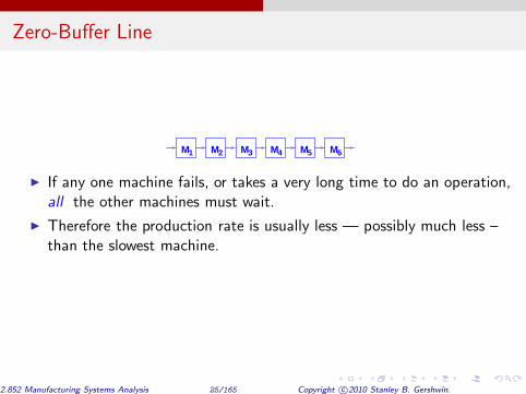
M1 M2 M3 4M M5 M6
◮ If any one machine fails, or takes a very long time to do an operation, all the other machines must wait.
◮ Therefore the production rate is usually less — possibly much less – than the slowest machine.
2.852 Manufacturing Systems Analysis 25/165 Copyright c©2010 Stanley B. Gershwin.

Zero-Buffer Line
M1 M2 M3 4M M5 M6
◮ Special case: Constant, unequal operation times, perfectly reliable machines.
◮ The operation time of the line is equal to the operation time of the slowest machine, so the production rate of the line is equal to that of the slowest machine.
2.852 Manufacturing Systems Analysis 26/165 Copyright c©2010 Stanley B. Gershwin.
Zero-Buffer Line Constant, equal operation times, unreliable machines
M1 M2 M3 4M M5 M6
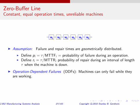
◮ Assumption: Failure and repair times are geometrically distributed.
◮ Define pi = τ/MTTFi = probability of failure during an operation. ◮ Define ri = τ/MTTRi probability of repair during an interval of length
τ when the machine is down.
◮ Operation-Dependent Failures (ODFs): Machines can only fail while they are working.
2.852 Manufacturing Systems Analysis 27/165 Copyright c©2010 Stanley B. Gershwin.

Zero-Buffer Line
M1 M2 M3 4M M5 M6
Buzacott’s Zero-Buffer Line Formula: Let k be the number of machines in the line. Then
P = 1
τ
1
1 + k ∑
i=1
pi
ri
2.852 Manufacturing Systems Analysis 28/165 Copyright c©2010 Stanley B. Gershwin.

Zero-Buffer Line
M1 M2 M3 4M M5 M6
◮ Same as the earlier formula (page 11, page 14) when k = 1. The isolated production rate of a single machine Mi is
1
τ
( 1
1 + pi
ri
)
= 1
τ
( ri
ri + pi
)
.
2.852 Manufacturing Systems Analysis 29/165 Copyright c©2010 Stanley B. Gershwin.

Zero-Buffer Line Proof of formula
◮ Let τ (the operation time) be the time unit.
◮ Assumption: At most, one machine can be down.
◮ Consider a long time interval of length T τ during which Machine Mi
fails mi times (i = 1, . . . k). M3 M3M5 2 M1 M4M
All up Some machine down
◮ Without failures, the line would produce T parts.
2.852 Manufacturing Systems Analysis 30/165 Copyright c©2010 Stanley B. Gershwin.
Zero-Buffer Line
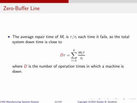
◮ The average repair time of Mi is τ/ri each time it fails, so the total system down time is close to
Dτ =
k ∑
i=1
miτ
ri
where D is the number of operation times in which a machine is down.
2.852 Manufacturing Systems Analysis 31/165 Copyright c©2010 Stanley B. Gershwin.
Zero-Buffer Line
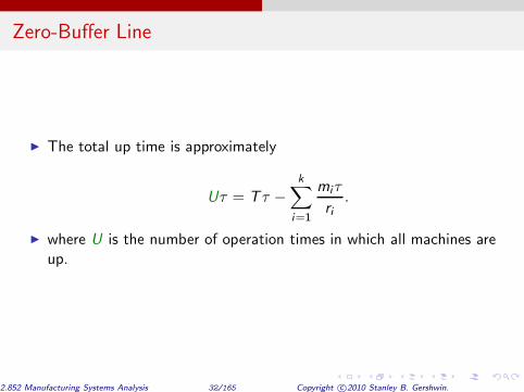
◮ The total up time is approximately
Uτ = T τ − k ∑
i=1
miτ
ri .
◮ where U is the number of operation times in which all machines are up.
2.852 Manufacturing Systems Analysis 32/165 Copyright c©2010 Stanley B. Gershwin.
Zero-Buffer Line
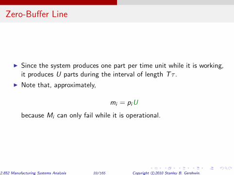
◮ Since the system produces one part per time unit while it is working, it produces U parts during the interval of length T τ .
◮ Note that, approximately,
mi = piU
because Mi can only fail while it is operational.
2.852 Manufacturing Systems Analysis 33/165 Copyright c©2010 Stanley B. Gershwin.

Zero-Buffer Line
◮ Thus,
Uτ = T τ − Uτ
k ∑
i=1
pi
ri ,
or,
U
T = EODF =
1
1 + k ∑
i=1
pi
ri
2.852 Manufacturing Systems Analysis 34/165 Copyright c©2010 Stanley B. Gershwin.

Zero-Buffer Line
and
P = 1
τ
1
1 +
k ∑
i=1
pi
ri
◮ Note that P is a function of the ratio pi/ri and not pi or ri separately.
◮ The same statement is true for the infinite-buffer line.
◮ However, the same statement is not true for a line with finite, non-zero buffers.
2.852 Manufacturing Systems Analysis 35/165 Copyright c©2010 Stanley B. Gershwin.

Zero-Buffer Line
Questions:
◮ If we want to increase production rate, which machine should we improve?
◮ What would happen to production rate if we improved any other machine?
2.852 Manufacturing Systems Analysis 36/165 Copyright c©2010 Stanley B. Gershwin.
Zero-Buffer Line ODF and TDF
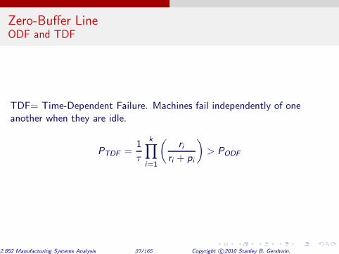
TDF= Time-Dependent Failure. Machines fail independently of one another when they are idle.
PTDF = 1
τ
k ∏
i=1
( ri
ri + pi
)
> PODF
2.852 Manufacturing Systems Analysis 37/165 Copyright c©2010 Stanley B. Gershwin.
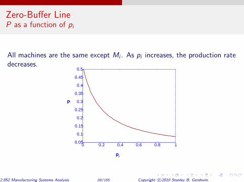
Zero-Buffer Line P as a function of pi
All machines are the same except Mi . As pi increases, the production rate decreases.
0 0.2 0.4 0.6 0.8 10.05
0.1
0.15
0.2
0.25
0.3
0.35
0.4
0.45
0.5
P
pi
2.852 Manufacturing Systems Analysis 38/165 Copyright c©2010 Stanley B. Gershwin.
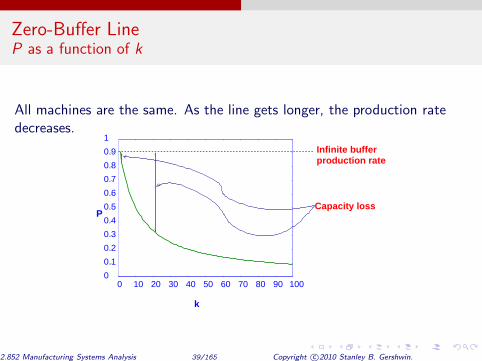
Zero-Buffer Line P as a function of k
All machines are the same. As the line gets longer, the production rate decreases.
0 10 20 30 40 50 60 70 80 90 100 0
0.1
0.2
0.3
0.4
0.5
0.6
0.7
0.8
0.9
1
k
P
Infinite buffer production rate
Capacity loss
2.852 Manufacturing Systems Analysis 39/165 Copyright c©2010 Stanley B. Gershwin.

Finite-Buffer Lines
M B1 1 M B2 2 M B3 3 M B4 4 M B5 5 M6
◮ Motivation for buffers: recapture some of the lost production rate.
◮ Cost ◮ in-process inventory/lead time ◮ floor space ◮ material handling mechanism
2.852 Manufacturing Systems Analysis 40/165 Copyright c©2010 Stanley B. Gershwin.

Finite-Buffer Lines
M B1 1 M B2 2 M B3 3 M B4 4 M B5 5 M6
◮ Infinite buffers: no propagation of disruptions.
◮ Zero buffers: instantaneous propagation.
◮ Finite buffers: delayed propagation. ◮ New phenomena: blockage and starvation .
2.852 Manufacturing Systems Analysis 41/165 Copyright c©2010 Stanley B. Gershwin.

Finite-Buffer Lines
M B1 1 M B2 2 M B3 3 M B4 4 M B5 5 M6
◮ Difficulty: ◮ No simple formula for calculating production rate or inventory levels.
◮ Solution: ◮ Simulation ◮ Analytical approximation
2.852 Manufacturing Systems Analysis 42/165 Copyright c©2010 Stanley B. Gershwin.
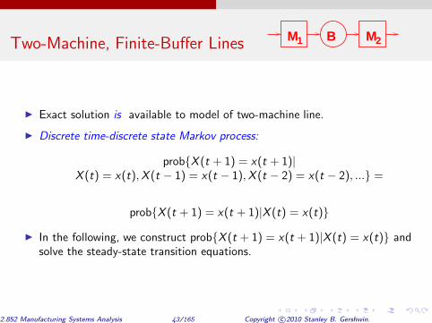
Two-Machine, Finite-Buffer Lines M1 M2B
◮ Exact solution is available to model of two-machine line.
◮ Discrete time-discrete state Markov process:
prob{X (t + 1) = x(t + 1)| X (t) = x(t), X (t − 1) = x(t − 1), X (t − 2) = x(t − 2), ...} =
prob{X (t + 1) = x(t + 1)|X (t) = x(t)}
◮ In the following, we construct prob{X (t + 1) = x(t + 1)|X (t) = x(t)} and solve the steady-state transition equations.
2.852 Manufacturing Systems Analysis 43/165 Copyright c©2010 Stanley B. Gershwin.

Two-Machine, Finite-Buffer Lines M1 M2B
Here, X (t) = (n(t), α1(t), α2(t)), where
◮ n is the number of parts in the buffer; n = 0, 1, ..., N.
◮ αi is the repair state of Mi ; i = 1, 2. ◮ αi = 1 means the machine is up or operational ; ◮ αi = 0 means the machine is down or under repair.
2.852 Manufacturing Systems Analysis 44/165 Copyright c©2010 Stanley B. Gershwin.
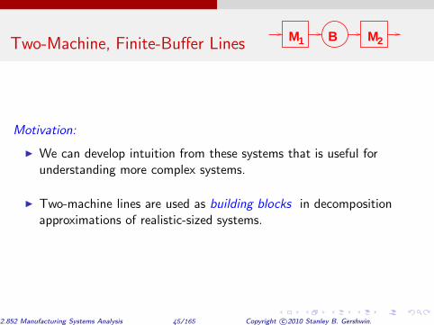
Two-Machine, Finite-Buffer Lines M1 M2B
Motivation:
◮ We can develop intuition from these systems that is useful for understanding more complex systems.
◮ Two-machine lines are used as building blocks in decomposition approximations of realistic-sized systems.
2.852 Manufacturing Systems Analysis 45/165 Copyright c©2010 Stanley B. Gershwin.

Two-Machine, Finite-Buffer Lines M1 M2B
Several models available:
◮ Deterministic processing time, or Buzacott model: deterministic processing time, geometric failure and repair times; discrete state, discrete time.
◮ Exponential processing time: exponential processing, failure, and repair time; discrete state, continuous time.
◮ Continuous material, or fluid: deterministic processing, exponential failure and repair time; mixed state, continuous time.
◮ Extensions ◮ Models with multiple up and down states.
2.852 Manufacturing Systems Analysis 46/165 Copyright c©2010 Stanley B. Gershwin.

Two-Machine, Finite-Buffer Lines M1 M2B
Outline: Details of two-machine, deterministic processing time line.
◮ Assumptions
◮ Performance measures
◮ Transient states
◮ Transition equations
◮ Identities
◮ Analytical solution
◮ Limits
◮ Behavior
2.852 Manufacturing Systems Analysis 47/165 Copyright c©2010 Stanley B. Gershwin.

Two-Machine, Finite-Buffer Lines M1 M2B
Assumptions, etc.
Assumptions, etc. for deterministic processing time systems (including long lines)
◮ All operation times are deterministic and equal to 1.
◮ The amount of material in Buffer i at time t is ni(t), 0 ≤ ni(t) ≤ Ni . A buffer gains or loses at most one piece during a time unit.
◮ The state of the system is s = (n1, . . . , nk−1, α1, . . . , αk).
2.852 Manufacturing Systems Analysis 48/165 Copyright c©2010 Stanley B. Gershwin.

Two-Machine, Finite-Buffer Lines M1 M2B
Assumptions, etc.
◮ Operation dependent failures:
prob [αi (t + 1) = 0 | ni−1(t) = 0, αi (t) = 1, ni (t) < Ni ] = 0, prob [αi (t + 1) = 1 | ni−1(t) = 0, αi (t) = 1, ni (t) < Ni ] = 1,
prob [αi (t + 1) = 0 | ni−1(t) > 0, αi (t) = 1, ni (t) = Ni ] = 0, prob [αi (t + 1) = 1 | ni−1(t) > 0, αi (t) = 1, ni (t) = Ni ] = 1,
prob [αi (t + 1) = 0 | ni−1(t) > 0, αi (t) = 1, ni (t) < Ni ] = pi , prob [αi (t + 1) = 1 | ni−1(t) > 0, αi (t) = 1, ni (t) < Ni ] = 1 − pi .
2.852 Manufacturing Systems Analysis 49/165 Copyright c©2010 Stanley B. Gershwin.

Two-Machine, Finite-Buffer Lines M1 M2B
Assumptions, etc.
◮ Repairs:
prob [αi(t + 1) = 1 | αi (t) = 0] = ri ,
prob [αi (t + 1) = 0 | αi (t) = 0] = 1 − ri .
2.852 Manufacturing Systems Analysis 50/165 Copyright c©2010 Stanley B. Gershwin.

Two-Machine, Finite-Buffer Lines M1 M2B
Assumptions, etc.
◮ Timing convention: In the absence of blocking or starvation:
ni (t + 1) = ni(t) + αi (t + 1) − αi+1(t + 1).
More generally,
ni(t + 1) = ni (t) + Iui (t + 1) − Idi(t + 1),
where
Iui (t + 1) =
{ 1 if αi (t + 1) = 1 and ni−1(t) > 0 and ni(t) < Ni ,
0 otherwise.
Idi (t + 1) =
{ 1 if αi+1(t + 1) = 1 and ni (t) > 0 and ni+1(t) < Ni+1
0 otherwise.
2.852 Manufacturing Systems Analysis 51/165 Copyright c©2010 Stanley B. Gershwin.

Two-Machine, Finite-Buffer Lines M1 M2B
Assumptions, etc.
◮ In the Markov chain model, there is a set of transient states, and a single final class. Thus, a unique steady state distribution exists. The model is studied in steady state. That is, we calculate the stationary probability distribution.
◮ We calculate performance measures (production rate and average inventory) from the steady state distribution.
2.852 Manufacturing Systems Analysis 52/165 Copyright c©2010 Stanley B. Gershwin.
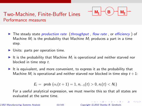
Two-Machine, Finite-Buffer Lines M1 M2B
Performance measures
◮ The steady state production rate (throughput , flow rate , or efficiency ) of Machine Mi is the probability that Machine Mi produces a part in a time step.
◮ Units: parts per operation time.
◮ It is the probability that Machine Mi is operational and neither starved nor blocked in time step t.
◮ It is equivalent, and more convenient, to express it as the probability that Machine Mi is operational and neither starved nor blocked in time step t + 1:
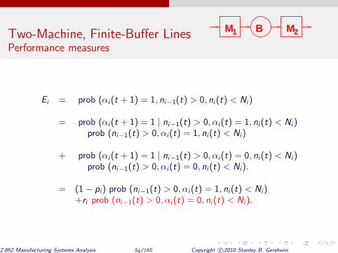
Ei = prob (αi (t + 1) = 1, ni−1(t) > 0, ni(t) < Ni )
For a useful analytical expression, we must rewrite this so that all states are evaluated at the same time.
2.852 Manufacturing Systems Analysis 53/165 Copyright c©2010 Stanley B. Gershwin.
Two-Machine, Finite-Buffer Lines M1 M2B
Performance measures
Ei = prob (αi (t + 1) = 1, ni−1(t) > 0, ni(t) < Ni)
= prob (αi (t + 1) = 1 | ni−1(t) > 0, αi(t) = 1, ni(t) < Ni ) prob (ni−1(t) > 0, αi(t) = 1, ni(t) < Ni)
+ prob (αi (t + 1) = 1 | ni−1(t) > 0, αi(t) = 0, ni(t) < Ni ) prob (ni−1(t) > 0, αi(t) = 0, ni(t) < Ni).
= (1 − pi) prob (ni−1(t) > 0, αi(t) = 1, ni(t) < Ni) +ri prob (ni−1(t) > 0, αi(t) = 0, ni(t) < Ni ).
2.852 Manufacturing Systems Analysis 54/165 Copyright c©2010 Stanley B. Gershwin.

Two-Machine, Finite-Buffer Lines M1 M2B
Performance measures
In steady state, there is a repair for every failure of Machine i , or
ri prob (ni−1(t) > 0, αi (t) = 0, ni (t) < Ni ) = pi prob (ni−1(t) > 0, αi (t) = 1, ni (t) < Ni )
Therefore,
Ei = prob (αi = 1, ni−1 > 0, ni < Ni ).
2.852 Manufacturing Systems Analysis 55/165 Copyright c©2010 Stanley B. Gershwin.
Two-Machine, Finite-Buffer Lines M1 M2B
Performance measures
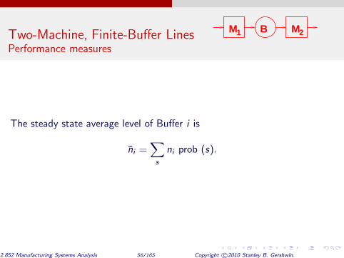
The steady state average level of Buffer i is
n̄i = ∑
s
ni prob (s).
2.852 Manufacturing Systems Analysis 56/165 Copyright c©2010 Stanley B. Gershwin.

Two-Machine, Finite-Buffer Lines M1 M2B
State Space
s = (n, α1, α2)
where
n = 0, 1, ..., N
αi = 0, 1
2.852 Manufacturing Systems Analysis 57/165 Copyright c©2010 Stanley B. Gershwin.
Two-Machine, Finite-Buffer Lines M1 M2B
Transient states
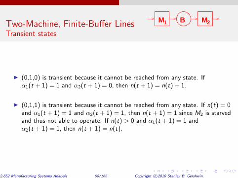
◮ (0,1,0) is transient because it cannot be reached from any state. If α1(t + 1) = 1 and α2(t + 1) = 0, then n(t + 1) = n(t) + 1.
◮ (0,1,1) is transient because it cannot be reached from any state. If n(t) = 0 and α1(t + 1) = 1 and α2(t + 1) = 1, then n(t + 1) = 1 since M2 is starved and thus not able to operate. If n(t) > 0 and α1(t + 1) = 1 and α2(t + 1) = 1, then n(t + 1) = n(t).
2.852 Manufacturing Systems Analysis 58/165 Copyright c©2010 Stanley B. Gershwin.

Two-Machine, Finite-Buffer Lines M1 M2B
Transient states
◮ (0,0,0) is transient because it can be reached only from itself or (0,1,0). It can be reached from itself if neither machine is repaired; it can be reached from (0,1,0) if the first machine fails while attempting to make a part. It cannot be reached from (0,0,1) or (0,1,1) since the second machine cannot fail. Otherwise, if α1(t + 1) = 0 and α2(t + 1) = 0, then n(t + 1) = n(t).
◮ (1,1,0) is transient because it can be reached only from (0,0,0) or (0,1,0). If α1(t + 1) = 1 and α2(t + 1) = 0, then n(t + 1) = n(t) + 1. Therefore, n(t) = 0. However, (1,1,0) cannot be reached from (0,0,1) since Machine 2 cannot fail. (For the same reason, it cannot be reached from (0,1,1), but since the latter is transient, that is irrelevant.)
◮ Similarly, (N, 0, 0), (N, 0, 1), (N, 1, 1), and (N − 1, 0, 1) are transient.
2.852 Manufacturing Systems Analysis 59/165 Copyright c©2010 Stanley B. Gershwin.

Two-Machine, Finite-Buffer Lines M1 M2B
State space
out of transient states
transitions
out of non−transient states
to increasing buffer level
to decreasing buffer level
unchanging buffer level
key
states
transient
non−transient
boundary
internal
n=2 n=3
1 2
(0,0)
(0,1)
(1,1)
(1,0)
n=4 n=5 n=6n=0 n=1 n=7 n=8 n=9 n=10 n=11 n=13
(α ,α ) =N
n=12 =N−1
2.852 Manufacturing Systems Analysis 60/165 Copyright c©2010 Stanley B. Gershwin.
Two-Machine, Finite-Buffer Lines M1 M2B
Transition equations
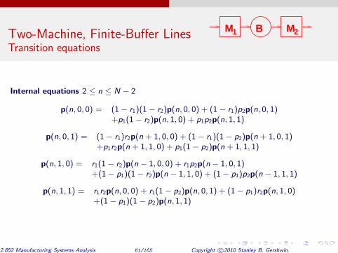
Internal equations 2 ≤ n ≤ N − 2
p(n, 0, 0) = (1 − r1)(1 − r2)p(n, 0, 0) + (1 − r1)p2p(n, 0, 1) +p1(1 − r2)p(n, 1, 0) + p1p2p(n, 1, 1)
p(n, 0, 1) = (1 − r1)r2p(n + 1, 0, 0) + (1 − r1)(1 − p2)p(n + 1, 0, 1) +p1r2p(n + 1, 1, 0) + p1(1 − p2)p(n + 1, 1, 1)
p(n, 1, 0) = r1(1 − r2)p(n − 1, 0, 0) + r1p2p(n − 1, 0, 1) +(1 − p1)(1 − r2)p(n − 1, 1, 0) + (1 − p1)p2p(n − 1, 1, 1)
p(n, 1, 1) = r1r2p(n, 0, 0) + r1(1 − p2)p(n, 0, 1) + (1 − p1)r2p(n, 1, 0) +(1 − p1)(1 − p2)p(n, 1, 1)
2.852 Manufacturing Systems Analysis 61/165 Copyright c©2010 Stanley B. Gershwin.

Two-Machine, Finite-Buffer Lines M1 M2B
Transition equations
Lower boundary equations n ≤ 1
p(0, 0, 1) = (1 − r1)p(0, 0, 1) + (1 − r1)r2p(1, 0, 0) +(1 − r1)(1 − p2)p(1, 0, 1) + p1(1 − p2)p(1, 1, 1).
p(1, 0, 0) = (1 − r1)(1 − r2)p(1, 0, 0) + (1 − r1)p2p(1, 0, 1) + p1p2p(1, 1, 1)
p(1, 0, 1) = (1 − r1)r2p(2, 0, 0) + (1 − r1)(1 − p2)p(2, 0, 1)+ p1r2p(2, 1, 0) + p1(1 − p2)p(2, 1, 1)
p(1, 1, 1) = r1p(0, 0, 1) + r1r2p(1, 0, 0) + r1(1 − p2)p(1, 0, 1) +(1 − p1)(1 − p2)p(1, 1, 1)
p(2, 1, 0) = r1(1 − r2)p(1, 0, 0) + r1p2p(1, 0, 1) + (1 − p1)p2p(1, 1, 1)
2.852 Manufacturing Systems Analysis 62/165 Copyright c©2010 Stanley B. Gershwin.

Two-Machine, Finite-Buffer Lines M1 M2B
Transition equations
Upper boundary equations n ≥ N − 1
p(N − 2, 0, 1) = (1 − r1)r2p(N − 1, 0, 0) + p1r2p(N − 1, 1, 0) +p1(1 − p2)p(N − 1, 1, 1)
p(N − 1, 0, 0) = (1 − r1)(1 − r2)p(N − 1, 0, 0) + p1(1 − r2)p(N − 1, 1, 0) +p1p2p(N − 1, 1, 1)
p(N − 1, 1, 0) = r1(1 − r2)p(N − 2, 0, 0) + r1p2p(N − 2, 0, 1) + (1 − p1)(1 − r2)p(N − 2, 1, 0) + (1 − p1)p2p(N − 2, 1, 1)
p(N − 1, 1, 1) = r1r2p(N − 1, 0, 0) + (1 − p1)r2p(N − 1, 1, 0) +(1 − p1)(1 − p2)p(N − 1, 1, 1) + r2p(N, 1, 0)
p(N, 1, 0) = r1(1 − r2)p(N − 1, 0, 0) + (1 − p1)(1 − r2)p(N − 1, 1, 0) +(1 − p1)p2p(N − 1, 1, 1) + (1 − r2)p(N, 1, 0)
2.852 Manufacturing Systems Analysis 63/165 Copyright c©2010 Stanley B. Gershwin.
Two-Machine, Finite-Buffer Lines M1 M2B
Performance measures
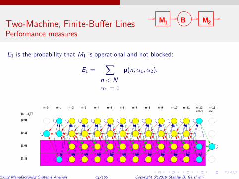
E1 is the probability that M1 is operational and not blocked:
E1 = ∑
n < N α1 = 1
p(n, α1, α2).
n=2 n=3
1 2
(0,0)
(0,1)
(1,1)
(1,0)
n=4 n=5 n=6n=0 n=1 n=7 n=8 n=9 n=10 n=11 n=13
(α ,α ) =N
n=12 =N−1
2.852 Manufacturing Systems Analysis 64/165 Copyright c©2010 Stanley B. Gershwin.

Two-Machine, Finite-Buffer Lines M1 M2B
Performance measures
E2 is the probability that M2 is operational and not starved:
E2 = ∑
n > 0 α2 = 1
p(n, α1, α2).
n=2 n=3
1 2
(0,0)
(0,1)
(1,1)
(1,0)
n=4 n=5 n=6n=0 n=1 n=7 n=8 n=9 n=10 n=11 n=13
(α ,α ) =N
n=12 =N−1
2.852 Manufacturing Systems Analysis 65/165 Copyright c©2010 Stanley B. Gershwin.

Two-Machine, Finite-Buffer Lines M1 M2B
Performance measures
The probabilities of starvation and blockage are:
ps = p(0, 0, 1), the probability of starvation,
pb = p(N , 1, 0), the probability of blockage.
The average buffer level is:
n̄ = ∑
all s
np(n, α1, α2).
2.852 Manufacturing Systems Analysis 66/165 Copyright c©2010 Stanley B. Gershwin.
Two-Machine, Finite-Buffer Lines M1 M2B
Identities
Repair frequency equals failure frequency For every repair, there is a failure (in steady state). When the system is in steady state,
r1 prob [{α1 = 0} and {n < N}] = p1 prob [{α1 = 1} and {n < N}] .
Let
D1 = prob [{α1 = 0} and {n < N}] ,
then
r1D1 = p1E1.
2.852 Manufacturing Systems Analysis 67/165 Copyright c©2010 Stanley B. Gershwin.

Two-Machine, Finite-Buffer Lines M1 M2B
Identities
Proof: The left side is the probability that the state leaves the set of states
S0 = {{α1 = 0} and {n < N}} .
since the only way the system can leave S0 is for M1 to get repaired. (M1 is down, so the buffer cannot become full.)
n=2 n=3
1 2
(0,0)
(0,1)
(1,1)
(1,0)
n=4 n=5 n=6n=0 n=1 n=7 n=8 n=9 n=10 n=11 n=13
(α ,α ) =N
n=12 =N−1
2.852 Manufacturing Systems Analysis 68/165 Copyright c©2010 Stanley B. Gershwin.

Two-Machine, Finite-Buffer Lines M1 M2B
Identities
The right side is the probability that the state enters S0. When the system is in steady state, the only way for the state to enter S0 is for it to be in set
S1 = {{α1 = 1} and {n < N}}
in the previous time unit. n=2 n=3
1 2
(0,0)
(0,1)
(1,1)
(1,0)
n=4 n=5 n=6n=0 n=1 n=7 n=8 n=9 n=10 n=11 n=13
(α ,α ) =N
n=12 =N−1
2.852 Manufacturing Systems Analysis 69/165 Copyright c©2010 Stanley B. Gershwin.

Two-Machine, Finite-Buffer Lines M1 M2B
Identities
Conservation of Flow E1 = E2 = E
Proof: E1 =
N−1 ∑
n=0
p(n, 1, 0) +
N−1 ∑
n=0
p(n, 1, 1),
E2 =
N ∑
n=1
p(n, 0, 1) +
N ∑
n=1
p(n, 1, 1).
Then E1 − E2 = N−1 ∑
n=0
p(n, 1, 0)− N ∑
n=1
p(n, 0, 1)
= N−2 ∑
n=1
p(n + 1, 1, 0)− N−2 ∑
n=1
p(n, 0, 1)
2.852 Manufacturing Systems Analysis 70/165 Copyright c©2010 Stanley B. Gershwin.

Two-Machine, Finite-Buffer Lines M1 M2B
Identities
Or,
E1 − E2 = N−2 ∑
n=1
( p(n + 1, 1, 0) − p(n, 0, 1)
)
Define δ(n) = p(n + 1, 1, 0) − p(n, 0, 1). Then
E1 − E2 =
N−2 ∑
n=1
δ(n)
2.852 Manufacturing Systems Analysis 71/165 Copyright c©2010 Stanley B. Gershwin.

Two-Machine, Finite-Buffer Lines M1 M2B
Identities
Add lots of lower boundary equations:
p(0, 0, 1) + p(1, 0, 0) + p(1, 1, 1) + p(2, 1, 0) =
(1 − r1)p(0, 0, 1) + (1 − r1)r2p(1, 0, 0) +(1 − r1)(1 − p2)p(1, 0, 1) + p1(1 − p2)p(1, 1, 1)
+(1 − r1)(1 − r2)p(1, 0, 0) + (1 − r1)p2p(1, 0, 1) + p1p2p(1, 1, 1)
+r1p(0, 0, 1) + r1r2p(1, 0, 0) + r1(1 − p2)p(1, 0, 1) +(1 − p1)(1 − p2)p(1, 1, 1)
+r1(1 − r2)p(1, 0, 0) + r1p2p(1, 0, 1) + (1 − p1)p2p(1, 1, 1)
2.852 Manufacturing Systems Analysis 72/165 Copyright c©2010 Stanley B. Gershwin.

Two-Machine, Finite-Buffer Lines M1 M2B
Identities
Or,
p(0, 0, 1) + p(1, 0, 0) + p(1, 1, 1) + p(2, 1, 0) =
p(0, 0, 1) + p(1, 0, 0) + p(1, 0, 1) + p(1, 1, 1)
Or,
p(2, 1, 0) = p(1, 0, 1)
Then δ(1) = 0.
2.852 Manufacturing Systems Analysis 73/165 Copyright c©2010 Stanley B. Gershwin.
Two-Machine, Finite-Buffer Lines M1 M2B
Identities
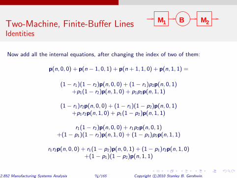
Now add all the internal equations, after changing the index of two of them:
p(n, 0, 0) + p(n − 1, 0, 1) + p(n + 1, 1, 0) + p(n, 1, 1) =
(1 − r1)(1 − r2)p(n, 0, 0) + (1 − r1)p2p(n, 0, 1) +p1(1 − r2)p(n, 1, 0) + p1p2p(n, 1, 1)
(1 − r1)r2p(n, 0, 0) + (1 − r1)(1 − p2)p(n, 0, 1) +p1r2p(n, 1, 0) + p1(1 − p2)p(n, 1, 1)
r1(1 − r2)p(n, 0, 0) + r1p2p(n, 0, 1) +(1 − p1)(1 − r2)p(n, 1, 0) + (1 − p1)p2p(n, 1, 1)
r1r2p(n, 0, 0) + r1(1 − p2)p(n, 0, 1) + (1 − p1)r2p(n, 1, 0) +(1 − p1)(1 − p2)p(n, 1, 1)
2.852 Manufacturing Systems Analysis 74/165 Copyright c©2010 Stanley B. Gershwin.

Two-Machine, Finite-Buffer Lines M1 M2B
Identities
Or, for n = 2, . . . , N − 2,
p(n, 0, 0) + p(n − 1, 0, 1) + p(n + 1, 1, 0) + p(n, 1, 1) =
p(n, 0, 0) + p(n, 0, 1) + p(n, 1, 0) + p(n, 1, 1),
or,
p(n + 1, 1, 0) − p(n, 0, 1) = p(n, 1, 0) − p(n − 1, 0, 1)
or, δ(n) = δ(n − 1)
2.852 Manufacturing Systems Analysis 75/165 Copyright c©2010 Stanley B. Gershwin.

Two-Machine, Finite-Buffer Lines M1 M2B
Identities
Since
δ(1) = 0 and δ(n) = δ(n − 1), n = 2, . . . , N − 2
we have
δ(n) = 0, n = 1, . . . , N − 2
Therefore
E1 − E2 = N−2 ∑
n=1
δ(n) = 0
QED
2.852 Manufacturing Systems Analysis 76/165 Copyright c©2010 Stanley B. Gershwin.

Two-Machine, Finite-Buffer Lines M1 M2B
Identities
Alternative interpretation of p(n + 1, 1, 0) − p(n, 0, 1) = 0:
n n+11 2
(0,0)
(0,1)
(1,1)
(1,0)
(α ,α ) ◮ The only way the buffer can go
from n + 1 to n is for the state to go to (n, 0, 1).
◮ The only way the buffer can go from n to n + 1 is for the state to go to (n + 1, 1, 0).
2.852 Manufacturing Systems Analysis 77/165 Copyright c©2010 Stanley B. Gershwin.
Two-Machine, Finite-Buffer Lines M1 M2B
Identities
Flow rate/idle time
E = e1(1 − pb).
Proof: From the definitions of E1 and D1, we have
prob [n < N] = E + D1,
or, 1−pb = E + p1
r1 E =
E
e1 .
Similarly,
E = e2(1 − ps)
2.852 Manufacturing Systems Analysis 78/165 Copyright c©2010 Stanley B. Gershwin.

Two-Machine, Finite-Buffer Lines M1 M2B
Analytical Solution
1. Guess a solution for the internal states of the form p(n, α1, α2) = ξj(n, α1, α2) = X nY α1
1 Y α2 2 .
2. Determine sets of Xj ,Y1j ,Y2j that satisfy the internal equations.
3. Extend ξj(n, α1, α2) to all of the boundary states using some of the boundary equations.
4. Find coefficients Cj so that p(n, α1, α2) = ∑
j Cjξj(n, α1, α2) satisfies the remaining boundary equationss and normalization.
2.852 Manufacturing Systems Analysis 79/165 Copyright c©2010 Stanley B. Gershwin.

Two-Machine, Finite-Buffer Lines M1 M2B
Analytical Solution
Internal equations:
X n = (1 − r1)(1 − r2)X n + (1 − r1)p2X nY2 + p1(1 − r2)X nY1 + p1p2X nY1Y2
X n−1Y2 = (1 − r1)r2X n + (1 − r1)(1 − p2)X nY2 + p1r2X nY1
+p1(1 − p2)X nY1Y2
X n+1Y1 = r1(1 − r2)X n + r1p2X nY2 + (1 − p1)(1 − r2)X nY1 + (1 − p1)p2X nY1Y2
X nY1Y2 = r1r2X n + r1(1 − p2)X nY2 + (1 − p1)r2X nY1 + (1 − p1)(1 − p2)X nY1Y2
2.852 Manufacturing Systems Analysis 80/165 Copyright c©2010 Stanley B. Gershwin.
Two-Machine, Finite-Buffer Lines M1 M2B
Analytical Solution
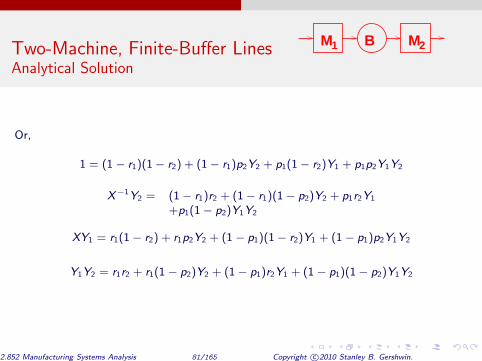
Or,
1 = (1 − r1)(1 − r2) + (1 − r1)p2Y2 + p1(1 − r2)Y1 + p1p2Y1Y2
X −1Y2 = (1 − r1)r2 + (1 − r1)(1 − p2)Y2 + p1r2Y1
+p1(1 − p2)Y1Y2
XY1 = r1(1 − r2) + r1p2Y2 + (1 − p1)(1 − r2)Y1 + (1 − p1)p2Y1Y2
Y1Y2 = r1r2 + r1(1 − p2)Y2 + (1 − p1)r2Y1 + (1 − p1)(1 − p2)Y1Y2
2.852 Manufacturing Systems Analysis 81/165 Copyright c©2010 Stanley B. Gershwin.

Two-Machine, Finite-Buffer Lines M1 M2B
Analytical Solution
Or,
1 = (1 − r1 + Y1p1) (1 − r2 + Y2p2)
X−1Y2 = (1 − r1 + Y1p1) (r2 + Y2(1 − p2))
XY1 = (r1 + Y1(1 − p1)) (1 − r2 + Y2p2)
Y1Y2 = (r1 + Y1(1 − p1)) (r2 + Y2(1 − p2))
2.852 Manufacturing Systems Analysis 82/165 Copyright c©2010 Stanley B. Gershwin.

Two-Machine, Finite-Buffer Lines M1 M2B
Analytical Solution
Since the last equation is a product of the other three, there are only three independent equations in three unknowns here. They may be simplified further:
1 = (1 − r1 + Y1p1) (1 − r2 + Y2p2)
XY1 = r1 + Y1(1 − p1)
1 − r1 + Y1p1
X−1Y2 = r2 + Y2(1 − p2)
1 − r2 + Y2p2
2.852 Manufacturing Systems Analysis 83/165 Copyright c©2010 Stanley B. Gershwin.
Two-Machine, Finite-Buffer Lines M1 M2B
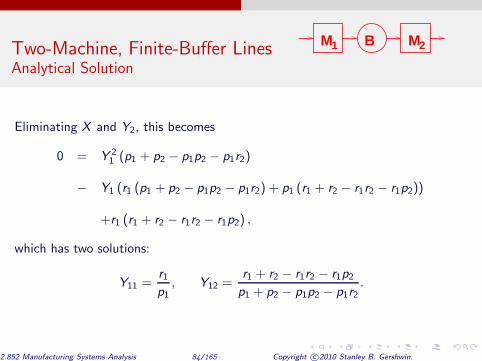
Analytical Solution
Eliminating X and Y2, this becomes
0 = Y 2 1 (p1 + p2 − p1p2 − p1r2)
− Y1 (r1 (p1 + p2 − p1p2 − p1r2) + p1 (r1 + r2 − r1r2 − r1p2))
+r1 (r1 + r2 − r1r2 − r1p2) ,
which has two solutions:
Y11 = r1 p1
, Y12 = r1 + r2 − r1r2 − r1p2
p1 + p2 − p1p2 − p1r2 .
2.852 Manufacturing Systems Analysis 84/165 Copyright c©2010 Stanley B. Gershwin.

Two-Machine, Finite-Buffer Lines M1 M2B
Analytical Solution
The complete solutions are:
Y11 = r1 p1
Y21 = r2 p2
X1 = 1
Y12 = r1 + r2 − r1r2 − r1p2
p1 + p2 − p1p2 − p1r2
Y22 = r1 + r2 − r1r2 − p1r2
p1 + p2 − p1p2 − p2r1
X2 = Y22
Y12
2.852 Manufacturing Systems Analysis 85/165 Copyright c©2010 Stanley B. Gershwin.

Two-Machine, Finite-Buffer Lines M1 M2B
Analytical Solution
Recall that ξ(n, α1, α2) = X nY α1 1 Y α2
2 .
We now have the complete internal solution:
p(n, α1, α2) = C1ξ1(n, α1, α2) + C2ξ2(n, α1, α2)
= C1Xn 1 Y
α1 11 Y
α2 21 + C2X
n 2 Y
α1 12 Y
α2 22 .
2.852 Manufacturing Systems Analysis 86/165 Copyright c©2010 Stanley B. Gershwin.
Two-Machine, Finite-Buffer Lines M1 M2B
Analytical Solution
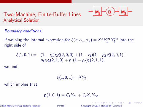
Boundary conditions:
If we plug the internal expression for ξ(n, α1, α2) = X nY α1 1 Y α2
2 into the right side of
ξ(1, 0, 1) = (1 − r1)r2ξ(2, 0, 0) + (1 − r1)(1 − p2)ξ(2, 0, 1)+ p1r2ξ(2, 1, 0) + p1(1 − p2)ξ(2, 1, 1),
we find
ξ(1, 0, 1) = XY2
which implies that
p(1, 0, 1) = C1Y21 + C2X2Y22.
2.852 Manufacturing Systems Analysis 87/165 Copyright c©2010 Stanley B. Gershwin.
Two-Machine, Finite-Buffer Lines M1 M2B
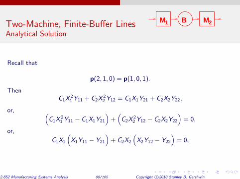
Analytical Solution
Recall that
p(2, 1, 0) = p(1, 0, 1).
Then C1X
2 1 Y11 + C2X
2 2 Y12 = C1X1Y21 + C2X2Y22,
or, ( C1X
2 1 Y11 − C1X1Y21
) + ( C2X
2 2 Y12 − C2X2Y22
) = 0,
or,
C1X1
( X1Y11 − Y21
) + C2X2
( X2Y12 − Y22
) = 0,
2.852 Manufacturing Systems Analysis 88/165 Copyright c©2010 Stanley B. Gershwin.

Two-Machine, Finite-Buffer Lines M1 M2B
Analytical Solution
Recall
X2 = Y22
Y12
Consequently,
C1X1
( X1Y11 − Y21
) = 0,
or,
C1
( r1
p1 −
r2
p2
)
= 0,
Therefore,
if r1
p1 6=
r2
p2 , then C1 = 0.
2.852 Manufacturing Systems Analysis 89/165 Copyright c©2010 Stanley B. Gershwin.

Two-Machine, Finite-Buffer Lines M1 M2B
Analytical Solution
In the following, we assume r1 p1
6= r2 p2
and we drop the j subscript.
But what happens when r1 p1
= r2 p2
?
And what does r1
p1 =
r2
p2 mean?
2.852 Manufacturing Systems Analysis 90/165 Copyright c©2010 Stanley B. Gershwin.
Two-Machine, Finite-Buffer Lines M1 M2B
Analytical Solution
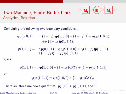
Combining the following two boundary conditions ...
r1p(0, 0, 1) = (1 − r1)r2p(1, 0, 0) + (1 − r1)(1 − p2)p(1, 0, 1)
+p1(1 − p2)p(1, 1, 1).
p(1, 1, 1) = r1p(0, 0, 1) + r1r2p(1, 0, 0) + r1(1 − p2)p(1, 0, 1) +(1 − p1)(1 − p2)p(1, 1, 1)
gives
p(1, 1, 1) = r2p(1, 0, 0) + (1 − p2)CXY2 + (1 − p2)p(1, 1, 1)
or, p2p(1, 1, 1) = r2p(1, 0, 0) + (1 − p2)CXY2.
There are three unknown quantities: p(1, 0, 0), p(1, 1, 1), and C .
2.852 Manufacturing Systems Analysis 91/165 Copyright c©2010 Stanley B. Gershwin.
Two-Machine, Finite-Buffer Lines M1 M2B
Analytical Solution
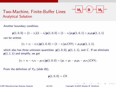
Another boundary condition,
p(1, 0, 0) = (1 − r1)(1 − r2)p(1, 0, 0) + (1 − r1)p2p(1, 0, 1) + p1p2p(1, 1, 1)
can be written
(r1 + r2 − r1r2)p(1, 0, 0) = (1 − r1)p2CXY2 + p1p2p(1, 1, 1).
which also has three unknown quantities: p(1, 0, 0), p(1, 1, 1), and C . If we eliminate p(1, 1, 1) and simplify, we get
(r1 + r2 − r1r2 − p1r2)p(1, 0, 0) = (p1 + p2 − p1p2 − p2r1)CXY2.
From the definition of Y22 (slide 85),
p(1, 0, 0) = CX .
2.852 Manufacturing Systems Analysis 92/165 Copyright c©2010 Stanley B. Gershwin.
Two-Machine, Finite-Buffer Lines M1 M2B
Analytical Solution
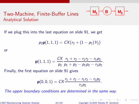
If we plug this into the last equation on slide 91, we get
p2p(1, 1, 1) = CX (r2 + (1 − p2)Y2)
or
p(1, 1, 1) = CX
p2
r1 + r2 − r1r2 − r1p2
p1 + p2 − p1p2 − r1p2 .
Finally, the first equation on slide 91 gives
p(0, 0, 1) = CX r1 + r2 − r1r2 − r1p2
r1p2 .
The upper boundary conditions are determined in the same way.
2.852 Manufacturing Systems Analysis 93/165 Copyright c©2010 Stanley B. Gershwin.
Two-Machine, Finite-Buffer Lines M1 M2B
Analytical Solution
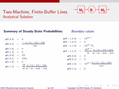
Summary of Steady-State Probabilities: Boundary values
p(0, 0, 0) = 0
p(0, 0, 1) = CX r1 + r2 − r1r2 − r1p2
r1p2
p(0, 1, 0) = 0
p(0, 1, 1) = 0
p(1, 0, 0) = CX
p(1, 0, 1) = CXY2
p(1, 1, 0) = 0
p(1, 1, 1) = CX
p2
r1 + r2 − r1r2 − r1p2
p1 + p2 − p1p2 − r1p2
p(N − 1, 0, 0) = CXN−1
p(N − 1, 0, 1) = 0
p(N − 1, 1, 0) = CXN−1
Y1
p(N − 1, 1, 1) = CXN−1
p1
r1 + r2 − r1r2 − p1r2
p1 + p2 − p1p2 − p1r2
p(N, 0, 0) = 0
p(N, 0, 1) = 0
p(N, 1, 0) = CXN−1 r1 + r2 − r1r2 − p1r2
p1r2
p(N, 1, 1) = 0
2.852 Manufacturing Systems Analysis 94/165 Copyright c©2010 Stanley B. Gershwin.

Two-Machine, Finite-Buffer Lines M1 M2B
Analytical Solution
Summary of Steady-State Probabilities: Internal states, etc.
p(n, α1, α2) = CX nY α1
1 Y α2
2 ,
2 ≤ n ≤ N − 2; α1 = 0, 1; α2 = 0, 1
where
Y1 = r1 + r2 − r1r2 − r1p2
p1 + p2 − p1p2 − p1r2
Y2 = r1 + r2 − r1r2 − p1r2
p1 + p2 − p1p2 − r1p2
X = Y2
Y1
and C is a normalizing constant.
2.852 Manufacturing Systems Analysis 95/165 Copyright c©2010 Stanley B. Gershwin.

Two-Machine, Finite-Buffer Lines M1 M2B
Analytical Solution
Observations:
Typically, we can expect that ri < .2 since a repair is likely to take at least 5 times as long as an operation. Also, since, typically, efficiency = ri/(ri + pi ) > .7, pi < .4ri , p(0, 0, 1), p(1, 1, 1), p(N − 1, 1, 1), p(N , 1, 0) are much larger than internal probabilities.
This is because the system tends to spend much more time at those states than at internal states.
Refer to transition graph on page 60 to trace out typical scenarios.
2.852 Manufacturing Systems Analysis 96/165 Copyright c©2010 Stanley B. Gershwin.

Two-Machine, Finite-Buffer Lines M1 M2B
Limits
If r1 → 0, then E → 0, ps → 1, pb → 0, n̄ → 0.
If r2 → 0, then E → 0, pb → 1, ps → 0, n̄ → N .
If p1 → 0, then ps → 0, E → 1 − pb → e2, n̄ → N − e2.
If p2 → 0, then pb → 0, E → 1 − ps → e1, n̄ → e1.
If N → ∞
and e1 < e2, then E → e1, pb → 0, ps → 1 − e1
e2 .
2.852 Manufacturing Systems Analysis 97/165 Copyright c©2010 Stanley B. Gershwin.
Two-Machine, Finite-Buffer Lines M1 M2B
Limits
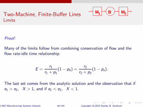
Proof:
Many of the limits follow from combining conservation of flow and the flow rate-idle time relationship:
E = r1
r1 + p1 (1 − pb) =
r2 r2 + p2
(1 − ps).
The last set comes from the analytic solution and the observation that if e1 > e2, X > 1, and if e1 < e2, X < 1.
2.852 Manufacturing Systems Analysis 98/165 Copyright c©2010 Stanley B. Gershwin.

Two-Machine, Finite-Buffer Lines M1 M2B
Behavior
0
2
4
6
8
10
0 200 400 600 800 1000
n(t)
t
r1 = .1, p1 = .01, r2 = .1, p2 = .01, N = 10
2.852 Manufacturing Systems Analysis 99/165 Copyright c©2010 Stanley B. Gershwin.

Two-Machine, Finite-Buffer Lines M1 M2B
Behavior
0
20
40
60
80
100
0 2000 4000 6000 8000 10000
n(t)
t
r1 = .1, p1 = .01, r2 = .1, p2 = .01, N = 100
2.852 Manufacturing Systems Analysis 100/165 Copyright c©2010 Stanley B. Gershwin.
Two-Machine, Finite-Buffer Lines M1 M2B
Behavior
0
20
40
60
80
100
0 2000 4000 6000 8000 10000
n(t)
t
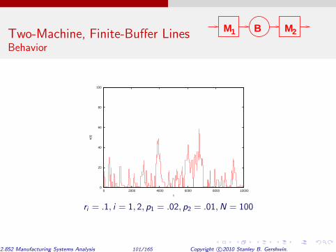
ri = .1, i = 1, 2, p1 = .02, p2 = .01, N = 100
2.852 Manufacturing Systems Analysis 101/165 Copyright c©2010 Stanley B. Gershwin.

Two-Machine, Finite-Buffer Lines M1 M2B
Behavior
0
20
40
60
80
100
0 2000 4000 6000 8000 10000
n(t)
t
ri = .1, i = 1, 2, p1 = .01, p2 = .02, N = 100
2.852 Manufacturing Systems Analysis 102/165 Copyright c©2010 Stanley B. Gershwin.

Two-Machine, Finite-Buffer Lines M1 M2B
Behavior
τ = 1. p1 = .1 r2 = .1 p2 = .1
Deterministic Processing Time
N
P
0 50 100 150 200
0.3
0.4
0.5
r = 0.06
r = 0.08
r = 0.1
r = 0.12
r = 0.14 11
1
1
1
1
1
2.852 Manufacturing Systems Analysis 103/165 Copyright c©2010 Stanley B. Gershwin.

Two-Machine, Finite-Buffer Lines M1 M2B
Behavior
Discussion:
◮ Why are the curves increasing?
◮ Why do they reach an asymptote?
◮ What is P when N = 0?
◮ What is the limit of P as N → ∞?
◮ Why are the curves with smaller r1 lower?
Deterministic Processing Time
N
P
0 50 100 150 200
0.3
0.4
0.5
r = 0.06
r = 0.08
r = 0.1
r = 0.12
r = 0.14 11
1
1
1
1
1
2.852 Manufacturing Systems Analysis 104/165 Copyright c©2010 Stanley B. Gershwin.

Two-Machine, Finite-Buffer Lines M1 M2B
Behavior
Discussion:
◮ Why are the curves increasing?
◮ Why different asymptotes?
◮ What is n̄ when N = 0?
◮ What is the limit of n̄ as N → ∞?
◮ Why are the curves with smaller r1 lower?
Deterministic Processing Time
N
n
0 50 100 150 200 0
50
100
150
200
r = 0.06
r = 0.08
r = 0.1
r = 0.12
r = 0.14 11
1
1
1
1
1
2.852 Manufacturing Systems Analysis 105/165 Copyright c©2010 Stanley B. Gershwin.

Two-Machine, Finite-Buffer Lines M1 M2B
Behavior
Deterministic Processing Time
N
P
0 50 100 150 200
0.3
0.4
0.5
r = 0.06
r = 0.08
r = 0.1
r = 0.12
r = 0.14 11
1
1
1
1
1
Deterministic Processing Time
N
n
0 50 100 150 200 0
50
100
150
200
r = 0.06
r = 0.08
r = 0.1
r = 0.12
r = 0.14 11
1
1
1
1
1
◮ What can you say about the optimal buffer size?
◮ How should it be related to ri , pi?
2.852 Manufacturing Systems Analysis 106/165 Copyright c©2010 Stanley B. Gershwin.
Two-Machine, Finite-Buffer Lines M1 M2B
Behavior
Questions:
◮ If we want to increase production rate, which machine should we improve?
◮ What would happen to production rate if we improved any other machine?
2.852 Manufacturing Systems Analysis 107/165 Copyright c©2010 Stanley B. Gershwin.
Two-Machine, Finite-Buffer Lines M1 M2B
Production rate vs. storage space
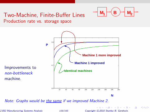
Improvements to non-bottleneck machine.
20 40 60 80 100 120 140 160 180 200 0.6
0.7
0.8
N
P
Identical machines
Machine 1 improved
Machine 1 more improved
Note: Graphs would be the same if we improved Machine 2.
2.852 Manufacturing Systems Analysis 108/165 Copyright c©2010 Stanley B. Gershwin.

Two-Machine, Finite-Buffer Lines M1 M2B
Average inventory vs. storage space
Inventory increases as the (non-bottleneck) upstream machine is improved and as the buffer space is increased.
0 20 40 60 80 100 120 140 160 180 200 0
20
40
60
80
100
120
140
160
180
200
n
N
Identical machines
Machine 1 more improved
improved Machine 1
2.852 Manufacturing Systems Analysis 109/165 Copyright c©2010 Stanley B. Gershwin.

Two-Machine, Finite-Buffer Lines M1 M2B
Average inventory vs. storage space
◮ Inventory decreases as the (non-bottleneck) downstream machine is improved.
◮ Inventory increases as the buffer space is increased.
20 40 60 80 100 120 140 160 180 200 0
20
40
60
80
100
120
140
160
180
200
Machine 2 more improved
n
N
Machine 2 improved Identical machines
2.852 Manufacturing Systems Analysis 110/165 Copyright c©2010 Stanley B. Gershwin.

Two-Machine, Finite-Buffer Lines M1 M2B
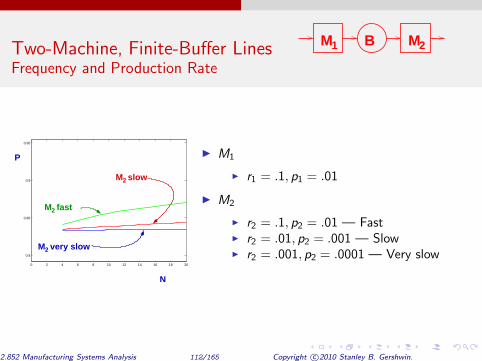
Frequency and Production Rate
Should we prefer short, frequent, disruptions or long, infrequent, disruptions?
◮ r2 = 0.8, p2 = 0.09, N = 10
◮ r1 and p1 vary together and r1 r1+p1
= .9
◮ Answer: evidently, short, frequent failures.
◮ Why?
r
P
0 0.2 0.4 0.6 0.8 1 0.75
0.8
0.85
0.9
0.95
1
2.852 Manufacturing Systems Analysis 111/165 Copyright c©2010 Stanley B. Gershwin.
Two-Machine, Finite-Buffer Lines M1 M2B
Frequency and Production Rate
0 2 4 6 8 10 12 14 16 18 20
0.8
0.85
0.9
0.95
P
N
2
2
2
M fast
M slow
M very slow
◮ M1
◮ r1 = .1, p1 = .01
◮ M2
◮ r2 = .1, p2 = .01 — Fast ◮ r2 = .01, p2 = .001 — Slow ◮ r2 = .001, p2 = .0001 — Very slow
2.852 Manufacturing Systems Analysis 112/165 Copyright c©2010 Stanley B. Gershwin.

Two-Machine, Finite-Buffer Lines M1 M2B
Frequency and Production Rate
0 20 40 60 80 100 120 140 160 180 200
0.8
0.85
0.9
0.95 ◮ M1
◮ r1 = .1, p1 = .01
◮ M2
◮ r2 = .1, p2 = .01 — Fast ◮ r2 = .01, p2 = .001 — Slow ◮ r2 = .001, p2 = .0001 — Very slow
2.852 Manufacturing Systems Analysis 113/165 Copyright c©2010 Stanley B. Gershwin.

Two-Machine, Finite-Buffer Lines M1 M2B
Frequency and Production Rate
0 200 400 600 800 1000 1200 1400 1600 1800 2000
0.8
0.85
0.9
0.95
◮ M1
◮ r1 = .1, p1 = .01
◮ M2
◮ r2 = .1, p2 = .01 — Fast ◮ r2 = .01, p2 = .001 — Slow ◮ r2 = .001, p2 = .0001 — Very slow
2.852 Manufacturing Systems Analysis 114/165 Copyright c©2010 Stanley B. Gershwin.

Two-Machine, Finite-Buffer Lines M1 M2B
Frequency and Production Rate
0 0.2 0.4 0.6 0.8 1 1.2 1.4 1.6 1.8 2
x 104
0.83
0.84
0.85
0.86
0.87
0.88
0.89
0.9
0.91
◮ M1
◮ r1 = .1, p1 = .01
◮ M2
◮ r2 = .1, p2 = .01 — Fast ◮ r2 = .01, p2 = .001 — Slow ◮ r2 = .001, p2 = .0001 — Very slow
2.852 Manufacturing Systems Analysis 115/165 Copyright c©2010 Stanley B. Gershwin.

Two-Machine, Finite-Buffer Lines M1 M2B
Frequency and Production Rate
0 1 2 3 4 5 6 7 8 9 10
x 104
0.8
0.85
0.9
0.95 ◮ M1
◮ r1 = .1, p1 = .01
◮ M2
◮ r2 = .1, p2 = .01 — Fast ◮ r2 = .01, p2 = .001 — Slow ◮ r2 = .001, p2 = .0001 — Very slow
2.852 Manufacturing Systems Analysis 116/165 Copyright c©2010 Stanley B. Gershwin.

Two-Machine, Finite-Buffer Lines M1 M2B
Frequency and Average Inventory
0 2 4 6 8 10 12 14 16 18 20 0
2
4
6
8
10
12
14
16
18
20
◮ M1
◮ r1 = .1, p1 = .01
◮ M2
◮ r2 = .1, p2 = .01 — Fast ◮ r2 = .01, p2 = .001 — Slow ◮ r2 = .001, p2 = .0001 — Very slow
2.852 Manufacturing Systems Analysis 117/165 Copyright c©2010 Stanley B. Gershwin.

Two-Machine, Finite-Buffer Lines M1 M2B
Frequency and Average Inventory
0 20 40 60 80 100 120 140 160 180 200 0
20
40
60
80
100
120
140
160
180
200
◮ M1
◮ r1 = .1, p1 = .01
◮ M2
◮ r2 = .1, p2 = .01 — Fast ◮ r2 = .01, p2 = .001 — Slow ◮ r2 = .001, p2 = .0001 — Very slow
2.852 Manufacturing Systems Analysis 118/165 Copyright c©2010 Stanley B. Gershwin.
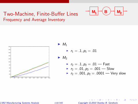
Two-Machine, Finite-Buffer Lines M1 M2B
Frequency and Average Inventory
0 200 400 600 800 1000 1200 1400 1600 1800 2000 0
200
400
600
800
1000
1200
1400
1600
1800
2000
◮ M1
◮ r1 = .1, p1 = .01
◮ M2
◮ r2 = .1, p2 = .01 — Fast ◮ r2 = .01, p2 = .001 — Slow ◮ r2 = .001, p2 = .0001 — Very slow
2.852 Manufacturing Systems Analysis 119/165 Copyright c©2010 Stanley B. Gershwin.

Two-Machine, Finite-Buffer Lines M1 M2B
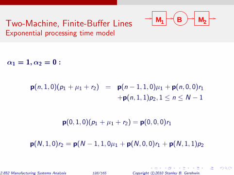
Exponential processing time model
Exponential processing time: exponential processing, failure, and repair time; discrete state, continuous time; discrete material.
Assumptions are similar to deterministic processing time model, except:
◮ µiδt = the probability that Mi completes an operation in (t, t + δt);
◮ piδt = the probability that Mi fails during an operation in (t, t + δt);
◮ riδt = the probability that Mi is repaired, while it is down, in (t, t + δt);
We can assume that only one event occurs during (t, t + δt).
2.852 Manufacturing Systems Analysis 120/165 Copyright c©2010 Stanley B. Gershwin.

Two-Machine, Finite-Buffer Lines M1 M2B
Exponential processing time model
n=2 n=3
1 2
(0,0)
(0,1)
(1,1)
(1,0)
n=4 n=5 n=6n=0 n=1 n=7 n=8 n=9 n=10 n=11 n=13
(α ,α ) =N
n=12 =N−1
transient
non−transient
boundary
internal
out of transient states
out of non−transient states
to increasing buffer level
to decreasing buffer level
unchanging buffer level
key
2.852 Manufacturing Systems Analysis 121/165 Copyright c©2010 Stanley B. Gershwin.
Two-Machine, Finite-Buffer Lines M1 M2B
Exponential processing time model
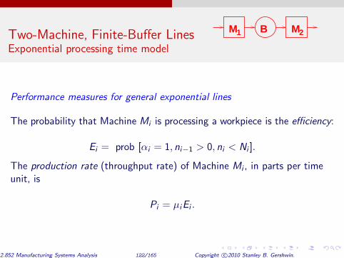
Performance measures for general exponential lines
The probability that Machine Mi is processing a workpiece is the efficiency:
Ei = prob [αi = 1, ni−1 > 0, ni < Ni ].
The production rate (throughput rate) of Machine Mi , in parts per time unit, is
Pi = µiEi .
2.852 Manufacturing Systems Analysis 122/165 Copyright c©2010 Stanley B. Gershwin.

Two-Machine, Finite-Buffer Lines M1 M2B
Exponential processing time model
Conservation of Flow
P = P1 = P2 = . . . = Pk .
This should be proved from the model.
2.852 Manufacturing Systems Analysis 123/165 Copyright c©2010 Stanley B. Gershwin.

Two-Machine, Finite-Buffer Lines M1 M2B
Exponential processing time model
Flow Rate-Idle Time Relationship
The isolated efficiency ei of Machine Mi is, as usual,
ei = ri
ri + pi
and it represents the fraction of time that Mi is operational. The isolated production rate is
ρi = µiei .
2.852 Manufacturing Systems Analysis 124/165 Copyright c©2010 Stanley B. Gershwin.
Two-Machine, Finite-Buffer Lines M1 M2B
Exponential processing time model
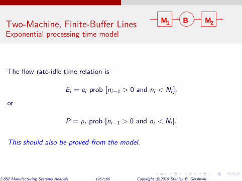
The flow rate-idle time relation is
Ei = ei prob [ni−1 > 0 and ni < Ni ].
or
P = ρi prob [ni−1 > 0 and ni < Ni ].
This should also be proved from the model.
2.852 Manufacturing Systems Analysis 125/165 Copyright c©2010 Stanley B. Gershwin.

Two-Machine, Finite-Buffer Lines M1 M2B
Exponential processing time model
Balance equations — steady state only
α1 = a2 = 0 :
p(n, 0, 0)(r1 + r2) = p(n, 1, 0)p1 + p(n, 0, 1)p2, 1 ≤ n ≤ N − 1,
p(0, 0, 0)(r1 + r2) = p(0, 1, 0)p1 ,
p(N, 0, 0)(r1 + r2) = p(N, 0, 1)p2 .
2.852 Manufacturing Systems Analysis 126/165 Copyright c©2010 Stanley B. Gershwin.

Two-Machine, Finite-Buffer Lines M1 M2B
Exponential processing time model
α1 = 0, α2 = 1 :
p(n, 0, 1)(r1 + µ2 + p2) = p(n, 0, 0)r2 + p(n, 1, 1)p1
+p(n + 1, 0, 1)µ2, 1 ≤ n ≤ N − 1
p(0, 0, 1)r1 = p(0, 0, 0)r2 + p(0, 1, 1)p1 + p(1, 0, 1)µ2
p(N, 0, 1)(r1 + µ2 + p2) = p(N, 0, 0)r2
2.852 Manufacturing Systems Analysis 127/165 Copyright c©2010 Stanley B. Gershwin.
Two-Machine, Finite-Buffer Lines M1 M2B
Exponential processing time model
α1 = 1, α2 = 0 :
p(n, 1, 0)(p1 + µ1 + r2) = p(n − 1, 1, 0)µ1 + p(n, 0, 0)r1
+p(n, 1, 1)p2, 1 ≤ n ≤ N − 1
p(0, 1, 0)(p1 + µ1 + r2) = p(0, 0, 0)r1
p(N, 1, 0)r2 = p(N − 1, 1, 0µ1 + p(N, 0, 0)r1 + p(N, 1, 1)p2
2.852 Manufacturing Systems Analysis 128/165 Copyright c©2010 Stanley B. Gershwin.

Two-Machine, Finite-Buffer Lines M1 M2B
Exponential processing time model
α1 = 1, α2 = 1 :
p(n, 1, 1)(p1 + p2 + µ1 + µ2) = p(n − 1, 1, 1)µ1 + p(n + 1, 1, 1)µ2
+p(n, 1, 0)r2 + p(n, 0, 1)r1, 1 ≤ n ≤ N − 1
p(0, 1, 1)(p1 + µ1) = p(1, 1, 1)µ2 + p(0, 1, 0)r2 + p(0, 0, 1)r1
p(N , 1, 1)(p2 + µ2) = p(N − 1, 1, 1)µ1 + p(N , 1, 0)r2 + p(N , 0, 1)r1
2.852 Manufacturing Systems Analysis 129/165 Copyright c©2010 Stanley B. Gershwin.

Two-Machine, Finite-Buffer Lines M1 M2B
Exponential processing time model
Performance measures
Efficiencies:
E1 = N−1 ∑
n=0
1 ∑
α2=0
p(n, 1, α2),
E2 = N ∑
n=1
1 ∑
α1=0
p(n, α1, 1).
2.852 Manufacturing Systems Analysis 130/165 Copyright c©2010 Stanley B. Gershwin.

Two-Machine, Finite-Buffer Lines M1 M2B
Exponential processing time model
Production rate:
P = µ1E1 = µ2E2.
Expected in-process inventory:
n̄ = N ∑
n=0
1 ∑
α1=0
1 ∑
α2=0
np(n, α1, α2).
2.852 Manufacturing Systems Analysis 131/165 Copyright c©2010 Stanley B. Gershwin.

Two-Machine, Finite-Buffer Lines M1 M2B
Solution of balance equations
Assume
p(n, α1, α2) = cX nY α1 1 Y α2
2 , 1 ≤ n ≤ N − 1
where c ,X ,Y1,Y2 are parameters to be determined. Plugging this into the internal equations gives
p1Y1 + p2Y2 − r1 − r2 = 0
µ1
( 1
X − 1
)
− p1Y1 + r1 + r1 Y1
− p1 = 0
µ2(X − 1) − p2Y2 + r2 Y2
+ r2 − p2 = 0
2.852 Manufacturing Systems Analysis 132/165 Copyright c©2010 Stanley B. Gershwin.

Two-Machine, Finite-Buffer Lines M1 M2B
Exponential processing time model
These equations can be reduced to one fourth-order polynomial (quartic) equation in one unknown. One solution is
Y11 = r1
p1
Y21 = r2
p2
X1 = 1
This solution of the quartic equation has a zero coefficient in the expression for the probabilities of the internal states:
p(n, α1, α2) =
4 ∑
j=1
cjXn j Y
α1
1j Y α2
2j for n = 1, . . . , N − 1.
The other three solutions satisfy a cubic polynomial equation. Compare with slide 85. In general, there is no simple expression for them.
2.852 Manufacturing Systems Analysis 133/165 Copyright c©2010 Stanley B. Gershwin.

Two-Machine, Finite-Buffer Lines M1 M2B
Exponential processing time model
Just as for the deterministic processing time line,
◮ we obtain the coefficients c1, c2, c3, c4 from the boundary conditions and the normalization equation;
◮ we find c1 = 0; (What does this mean? Why is this true?)
◮ we construct all the boundary probabilities. Some are 0.
◮ we use the probabilities to evaluate production rate, average buffer level, etc;
◮ we prove statements about conservation of flow, flow rate-idle time, limiting values of some quantities, etc.
◮ we draw graphs, and observe behavior which is qualitatively very similar to deterministic processing time line behavior (e.g., P vs. N, n̄ vs N, etc.).
We also draw some new graphs (P vs. µi , n̄ vs µi ) and observe new behavior. This is discussed below with the discussion of continuous material lines.
2.852 Manufacturing Systems Analysis 134/165 Copyright c©2010 Stanley B. Gershwin.

Two-Machine, Finite-Buffer Lines M1 M2B
Continuous Material model
Continuous material, or fluid: deterministic processing, exponential failure and repair time; mixed state, continuous time.; continuous material.
◮ µiδt = the amount of material that Mi processes, while it is up, in (t, t + δt);
◮ piδt = the probability that Mi fails, while it is up, in (t, t + δt);
◮ riδt = the probability that Mi is repaired, while it is down, in (t, t + δt);
2.852 Manufacturing Systems Analysis 135/165 Copyright c©2010 Stanley B. Gershwin.

Two-Machine, Finite-Buffer Lines M1 M2B
Model assumptions, notation, terminology, and conventions
During time interval (t, t + δt):
When 0 < x < N
1. the change in x is (α1µ1 − α2µ2)δt
2. the probability of repair of Machine i , that is, the probability that αi(t + δt) = 1 given that αi (t) = 0, is riδt
3. the probability of failure of Machine i , that is, the probability that αi(t + δt) = 0 given that αi (t) = 1, is piδt.
2.852 Manufacturing Systems Analysis 136/165 Copyright c©2010 Stanley B. Gershwin.

Two-Machine, Finite-Buffer Lines M1 M2B
When x = 0
1. the change in x is (α1µ1 − α2µ2)+δt
(That is, when x = 0, it can only increase.)
2. the probability of repair is riδt
3. if Machine 1 is down, Machine 2 cannot fail. If Machine 1 is up, the probability of failure of Machine 2 is pb
2δt, where
p b 2 =
p2µ
µ2 , µ = min(µ1, µ2)
The probability of failure of Machine 1 is p1δt.
2.852 Manufacturing Systems Analysis 137/165 Copyright c©2010 Stanley B. Gershwin.

Two-Machine, Finite-Buffer Lines M1 M2B
When x = N
1. the change in x is (α1µ1 − α2µ2)−δt
2. the probability of repair is riδt
3. if Machine 2 is down, Machine 1 cannot fail. If Machine 2 is up, the probability of failure of Machine 1 is pb
1δt, where
p b 1 =
p1µ
µ1 .
The probability of failure of Machine 2 is p2δt.
2.852 Manufacturing Systems Analysis 138/165 Copyright c©2010 Stanley B. Gershwin.

Two-Machine, Finite-Buffer Lines M1 M2B
Transition equations — internal
f (x , α1, α2, t)δx + o(δx) is the probability of the buffer level being between x and x + δx and the machines being in states α1 and α2 at time t.
δx
1 2 1 − (p +p ) tδ
µ δ 1
x −
t
µ δ 2
µ δ 1
x −
t +
t
µ δ 2
x
(0,1)
(0,0)
2δr t
1δr t
(1,1)
(1,0)
Transitions into ([x,x+ x],1,1)δ
2.852 Manufacturing Systems Analysis 139/165 Copyright c©2010 Stanley B. Gershwin.

Two-Machine, Finite-Buffer Lines M1 M2B
Then
f (x , 1, 1, t + δt) = (1 − (p1 + p2)δt)f (x − µ1δt + µ2δt, 1, 1, t)
+r1δtf (x + µ2δt, 0, 1, t) + r2δtf (x − µ1δt, 1, 0, t)
+o(δt)
or
f (x , 1, 1, t + δt) =
(1 − (p1 + p2)δt)
(
f (x , 1, 1, t) + ∂f
∂x (x , 1, 1, t)(−µ1δt + µ2δt)
)
+r1δtf (x + µ2δt, 0, 1, t) + r2δtf (x − µ1δt, 1, 0, t) + o(δt)
2.852 Manufacturing Systems Analysis 140/165 Copyright c©2010 Stanley B. Gershwin.
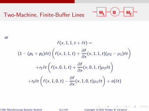
Two-Machine, Finite-Buffer Lines M1 M2B
or f (x , 1, 1, t + δt) =
(1 − (p1 + p2)δt)
(
f (x , 1, 1, t) + ∂f
∂x (x , 1, 1, t)(µ2 − µ1)δt
)
+r1δt
(
f (x , 0, 1, t) + ∂f
∂x (x , 0, 1, t)µ2δt
)
+r2δt
(
f (x , 1, 0, t) − ∂f
∂x (x , 1, 0, t)µ1δt
)
+ o(δt)
2.852 Manufacturing Systems Analysis 141/165 Copyright c©2010 Stanley B. Gershwin.

Two-Machine, Finite-Buffer Lines M1 M2B
or f (x , 1, 1, t + δt) =
f (x , 1, 1, t) − (p1 + p2)f (x , 1, 1, t)δt + (µ2 − µ1) ∂f
∂x (x , 1, 1, t)δt
+r1f (x , 0, 1, t)δt + r2f (x , 1, 0, t)δt
or, finally,
∂f
∂t (x , 1, 1) = −(p1 + p2)f (x , 1, 1) + (µ2 − µ1)
∂f
∂x (x , 1, 1)
+r1f (x , 0, 1) + r2f (x , 1, 0)
2.852 Manufacturing Systems Analysis 142/165 Copyright c©2010 Stanley B. Gershwin.
Two-Machine, Finite-Buffer Lines M1 M2B
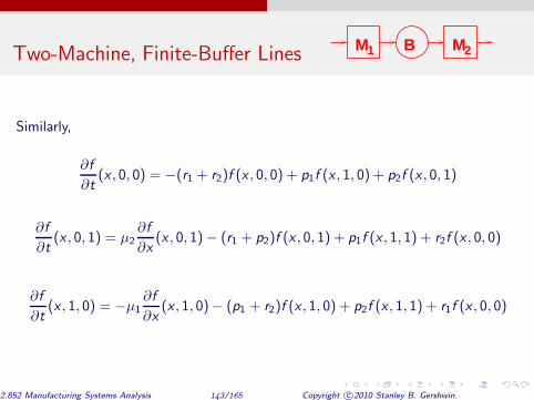
Similarly,
∂f
∂t (x , 0, 0) = −(r1 + r2)f (x , 0, 0) + p1f (x , 1, 0) + p2f (x , 0, 1)
∂f
∂t (x , 0, 1) = µ2
∂f
∂x (x , 0, 1) − (r1 + p2)f (x , 0, 1) + p1f (x , 1, 1) + r2f (x , 0, 0)
∂f
∂t (x , 1, 0) = −µ1
∂f
∂x (x , 1, 0)− (p1 + r2)f (x , 1, 0) + p2f (x , 1, 1) + r1f (x , 0, 0)
2.852 Manufacturing Systems Analysis 143/165 Copyright c©2010 Stanley B. Gershwin.

Two-Machine, Finite-Buffer Lines M1 M2B
Transition equations — boundary
p(x , α1, α2, t) is the probability of the buffer level being x (where x = 0 or N) and the machines being in states α1 and α2 at time t.
Boundary equations describe transitions from boundary states to boundary states; from boundary states to interior states; and from interior states to boundary states.
Boundary equations are relationships among p(x , α1, α2, t) and f (x , α1, α2, t) and their derivatives for x = 0 or x = N.
2.852 Manufacturing Systems Analysis 144/165 Copyright c©2010 Stanley B. Gershwin.
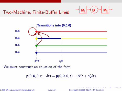
Two-Machine, Finite-Buffer Lines M1 M2B
(0,1)
x = 0
(1,1)
(1,0)
x = 0 µ δ
(0,0)
t2
Transitions into (0,0,0)
We must construct an equation of the form
p(0, 0, 0, t + δt) = p(0, 0, 0, t) + Aδt + o(δt)
2.852 Manufacturing Systems Analysis 145/165 Copyright c©2010 Stanley B. Gershwin.

Two-Machine, Finite-Buffer Lines M1 M2B
(0,1)
(0,0)
p t1δ1δr t + 2δr t1 −
(1,1)
(1,0)
x = 0
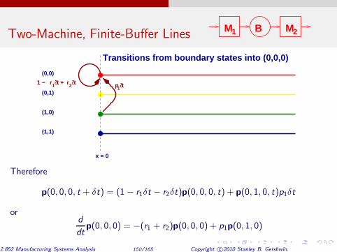
Transitions from boundary states into (0,0,0)
The system can go from (0,0,0) to (0,0,0) if there is no repair. It can go from (0,1,0) if the first machine does not fail.
It cannot go from (0,0,1) to (0,0,0) because the second machine is starved and
cannot fail. To go from (0,1,1) to (0,0,0) require two simultaneous failures, which
has a probability on the order of δt2 .
2.852 Manufacturing Systems Analysis 146/165 Copyright c©2010 Stanley B. Gershwin.
Two-Machine, Finite-Buffer Lines M1 M2B
(0,1)
(0,0)
(1,1)
(1,0)
x = 0 µ δ
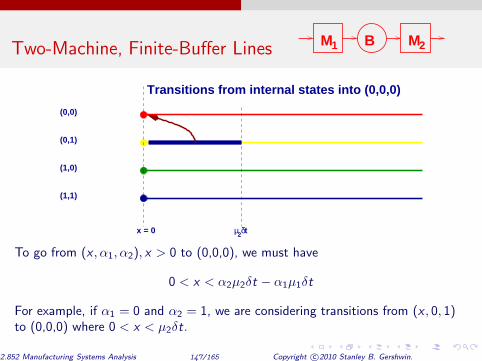
Transitions from internal states into (0,0,0)
t2
To go from (x , α1, α2), x > 0 to (0,0,0), we must have
0 < x < α2µ2δt − α1µ1δt
For example, if α1 = 0 and α2 = 1, we are considering transitions from (x , 0, 1) to (0,0,0) where 0 < x < µ2δt.
2.852 Manufacturing Systems Analysis 147/165 Copyright c©2010 Stanley B. Gershwin.

Two-Machine, Finite-Buffer Lines M1 M2B
(0,1)
(0,0)
(1,1)
(1,0)
x = 0 µ δ
Transitions from internal states into (0,0,0)
t2
But
prob ([0 < x < µ2δt], 0, 1) = f (x , 0, 1)µ2δt + o(δt) = f (0, 0, 1)µ2δt + o(δt)
and the transition probability from (0,1) to (0,0) is
(1 − r1δt)p2δt + o(δt) = p2δt + o(δt).
2.852 Manufacturing Systems Analysis 148/165 Copyright c©2010 Stanley B. Gershwin.

Two-Machine, Finite-Buffer Lines M1 M2B
(0,1)
(0,0)
(1,1)
(1,0)
x = 0 µ δ
Transitions from internal states into (0,0,0)
t2
Therefore, the probability of going from ([0 < x < µ2δt], 0, 1) to (0,0,0) is
f (x , 0, 1)µ2p2δt2 + (δt)o(δt) = o(δt)
For other transitions from (x , α1, α2), x > 0 to (0,0,0), the probabilities are similar or smaller.
2.852 Manufacturing Systems Analysis 149/165 Copyright c©2010 Stanley B. Gershwin.
Two-Machine, Finite-Buffer Lines M1 M2B
(0,1)
(0,0)
p t1δ1δr t + 2δr t1 −
(1,1)
(1,0)
x = 0
Transitions from boundary states into (0,0,0)
Therefore
p(0, 0, 0, t + δt) = (1 − r1δt − r2δt)p(0, 0, 0, t) + p(0, 1, 0, t)p1δt
or d
dtp(0, 0, 0) = −(r1 + r2)p(0, 0, 0) + p1p(0, 1, 0)
2.852 Manufacturing Systems Analysis 150/165 Copyright c©2010 Stanley B. Gershwin.
Two-Machine, Finite-Buffer Lines M1 M2B
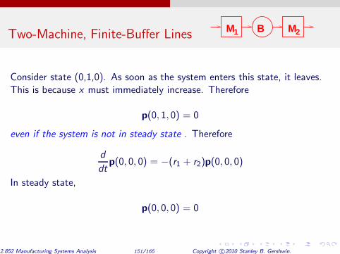
Consider state (0,1,0). As soon as the system enters this state, it leaves. This is because x must immediately increase. Therefore
p(0, 1, 0) = 0
even if the system is not in steady state . Therefore
d
dtp(0, 0, 0) = −(r1 + r2)p(0, 0, 0)
In steady state,
p(0, 0, 0) = 0
2.852 Manufacturing Systems Analysis 151/165 Copyright c©2010 Stanley B. Gershwin.

r 2
Two-Machine, Finite-Buffer Lines M1 M2B
(0,1)
(0,0)
1δr t1 −
p t1δ
tδ
µ δ
(1,1)
(1,0)
x = 0
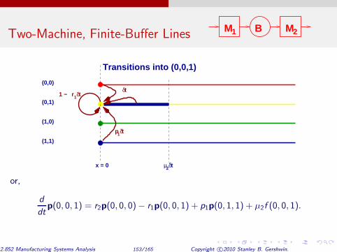
Transitions into (0,0,1)
t2
p(0, 0, 1, t + δt) = r2δtp(0, 0, 0, t) + (1 − r1δt)p(0, 0, 1, t)
+p1δtp(0, 1, 1, t) +
∫ µ2δt
0
f (x , 0, 1, t)dx
2.852 Manufacturing Systems Analysis 152/165 Copyright c©2010 Stanley B. Gershwin.
r 2
Two-Machine, Finite-Buffer Lines M1 M2B
(0,1)
(0,0)
1δr t1 −
p t1δ
tδ
µ δ
(1,1)
(1,0)
x = 0
Transitions into (0,0,1)
t2
or,
d
dtp(0, 0, 1) = r2p(0, 0, 0)− r1p(0, 0, 1) + p1p(0, 1, 1) + µ2f (0, 0, 1).
2.852 Manufacturing Systems Analysis 153/165 Copyright c©2010 Stanley B. Gershwin.
Two-Machine, Finite-Buffer Lines M1 M2B
µ > µ
r t1δ
(0,0)
(0,1)
1δp t +1 − δp t2
b
(µ − µ )δ
(1,1)
(1,0)
x = 0
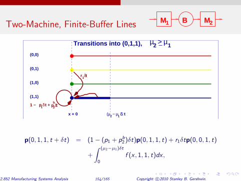
Transitions into (0,1,1),
2 t1
12
p(0, 1, 1, t + δt) = (1 − (p1 + p b 2 )δt)p(0, 1, 1, t) + r1δtp(0, 0, 1, t)
+
∫ (µ2−µ1)δt
0
f (x , 1, 1, t)dx ,
2.852 Manufacturing Systems Analysis 154/165 Copyright c©2010 Stanley B. Gershwin.
Two-Machine, Finite-Buffer Lines M1 M2B
µ > µ
r t1δ
(0,0)
(0,1)
1δp t +1 − δp t2
b
(µ − µ )δ
(1,1)
(1,0)
x = 0
Transitions into (0,1,1),
2 t1
12
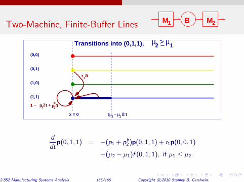
d
dtp(0, 1, 1) = −(p1 + p b
2 )p(0, 1, 1) + r1p(0, 0, 1)
+(µ2 − µ1)f (0, 1, 1), if µ1 ≤ µ2.
2.852 Manufacturing Systems Analysis 155/165 Copyright c©2010 Stanley B. Gershwin.

Two-Machine, Finite-Buffer Lines M1 M2B
Transitions into (0,1,1), µ2 ≤ µ1
If x(t) = 0, the transition from any (α1(t), α2(t)) to (α1(t + δt), α2(t + δt)) = (1, 1) would cause x to increase immediately. Therefore
p(0, 1, 1) = 0
2.852 Manufacturing Systems Analysis 156/165 Copyright c©2010 Stanley B. Gershwin.

Two-Machine, Finite-Buffer Lines M1 M2B
To come:
◮ Other boundary equations
◮ Normalization
1 X
α1=0
1 X
α2=0
»Z N
0
f (x , α1, α2)dx + p(0, α1, α2) + p(N, α1, α2)
–
= 1.
◮ Production rate
P2 = µ2
»Z N
0
(f (x , 0, 1) + f (x , 1, 1))dx + p(N, 1, 1)
–
+ µ1p(0, 1, 1).
= P1 = µ1
»Z N
0
(f (x , 1, 0) + f (x , 1, 1))dx + p(0, 1, 1)
–
+ µ2p(N, 1, 1).
◮ Average in-process inventory
x̄ =
1 X
α1=0
1 X
α2=0
»Z N
0
xf (x , α1, α2)dx + Np(N, α1, α2)
–
.
2.852 Manufacturing Systems Analysis 157/165 Copyright c©2010 Stanley B. Gershwin.
Two-Machine, Finite-Buffer Lines M1 M2B
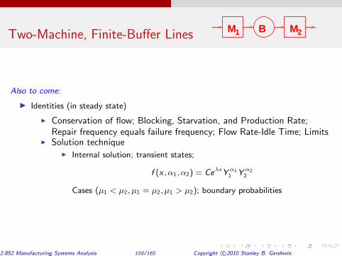
Also to come:
◮ Identities (in steady state)
◮ Conservation of flow; Blocking, Starvation, and Production Rate; Repair frequency equals failure frequency; Flow Rate-Idle Time; Limits
◮ Solution technique ◮ Internal solution; transient states;
f (x , α1, α2) = Ceλx Y α1 1 Y α2
2
Cases (µ1 < µ2, µ1 = µ2, µ1 > µ2); boundary probabilities
2.852 Manufacturing Systems Analysis 158/165 Copyright c©2010 Stanley B. Gershwin.
Two-Machine, Finite-Buffer Lines M1 M2B
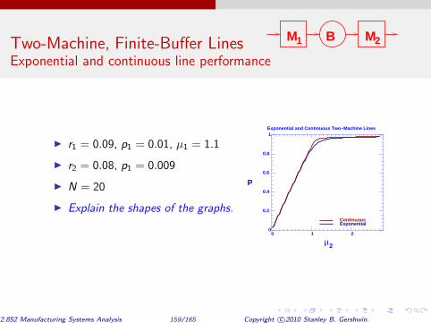
Exponential and continuous line performance
◮ r1 = 0.09, p1 = 0.01, µ1 = 1.1
◮ r2 = 0.08, p1 = 0.009
◮ N = 20
◮ Explain the shapes of the graphs.
Exponential and Continuous Two−Machine Lines
µ
P
0 1 2 0
0.2
0.4
0.6
0.8
1
Exponential Continuous
2
2.852 Manufacturing Systems Analysis 159/165 Copyright c©2010 Stanley B. Gershwin.
Two-Machine, Finite-Buffer Lines M1 M2B
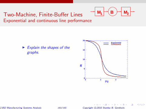
Exponential and continuous line performance
◮ Explain the shapes of the graphs.
µ
n
0 1 2 0
5
10
15
20 ExponentialContinuous
2
2.852 Manufacturing Systems Analysis 160/165 Copyright c©2010 Stanley B. Gershwin.

Two-Machine, Finite-Buffer Lines M1 M2B
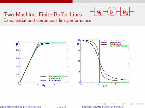
Exponential and continuous line performance
The no-variability limit: Consider a new continuous-material two-machine line. It is has parameters µ ′ 1, r
′
1, p ′ 1, µ ′ 2, r ′
2, p ′ 2, N′ . Assume it is perfectly reliable and its machines have the
same isolated production rates as those of the first continuous-material two-machine line. It also has the same buffer size. Its parameters are therefore given by
µ ′ 1 = ρ1; r ′ 1 unspecified; p ′ 1 = 0; N ′ = N µ ′ 2 = ρ2; r ′ 2 unspecified; p ′ 2 = 0
where ρi = µi
ri ri + pi
2.852 Manufacturing Systems Analysis 161/165 Copyright c©2010 Stanley B. Gershwin.
Two-Machine, Finite-Buffer Lines M1 M2B
Exponential and continuous line performance
µ
P
0 1 2 0
0.2
0.4
0.6
0.8
1
Exponential Continuous No−variability limit
2 µ
n
0 1 2 0
5
10
15
20 Exponential
No−variability limit Continuous
2
2.852 Manufacturing Systems Analysis 162/165 Copyright c©2010 Stanley B. Gershwin.
Two-Machine, Finite-Buffer Lines M1 M2B
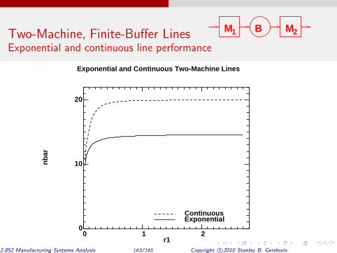
Exponential and continuous line performance
Exponential and Continuous Two-Machine Lines
r1
nb
ar
0 1 2 0
10
20
Exponential Continuous
2.852 Manufacturing Systems Analysis 163/165 Copyright c©2010 Stanley B. Gershwin.
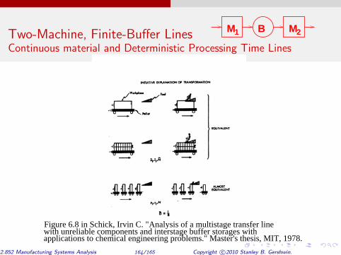
Two-Machine, Finite-Buffer Lines M1 M2B
Continuous material and Deterministic Processing Time Lines
2.852 Manufacturing Systems Analysis 164/165 Copyright c©2010 Stanley B. Gershwin.
Figure 6.8 in Schick, Irvin C. "Analysis of a multistage transfer line with unreliable components and interstage buffer storages with applications to chemical engineering problems." Master's thesis, MIT, 1978.

Two-Machine, Finite-Buffer Lines M1 M2B
Continuous material and Deterministic Processing Time Lines
delta transformation
delta
E
0 0.2 0.4 0.6 0.8 1 0.655
0.66
0.665
0.67
2.852 Manufacturing Systems Analysis 165/165 Copyright c©2010 Stanley B. Gershwin.

For information about citing these materials or our Terms of Use, visit: http://ocw.mit.edu/terms.
MIT OpenCourseWare http://ocw.mit.edu
2.852 Manufacturing Systems Analysis Spring 2010
For information about citing these materials or our Terms of Use,visit:http://ocw.mit.edu/terms.