missouri river freight corridor assessment and … · this report identifies the addressable market...
TRANSCRIPT
Supporting Document Prepared for Missouri Department of Transportation 2011 October Project TRyy1018 Report cmr 12 - 006
Missouri River Freight Corridor Assessment and Development Plan
Market Potential
(Technical Memo 3)
Prepared By
Hanson Professional Services, Inc.

Hanson Professional Services Inc.
Missouri River Freight Corridor Assessment & Development Plan Missouri Department of Transportation
Preface
Preface Task 3 consisted of collecting freight data information to develop a “baseline” condition for shipping to and from the Missouri River region. Both domestic and international data were gathered for freight moving to and from Missouri by port, trade region, and commodity value to develop a model for Missouri trade. This model serves as a point of reference to analyze the relative freight volume shares of exports and imports of rail and truck by port and commodity. This effort included:
• The examination and summarization of freight movements to and from the Missouri River Corridor to identify commodity groups (and associated traffic levels) that might be suitable for a shift in transportation mode as well as market locations most likely to shift to water from another mode.
• Analysis of growth projections and trade trends for the potential waterborne
freight types.
The resulting effort provides a background understanding of the potential freight markets, volumes, locations, and general logistical needs of the Missouri River region. This information is part of establishing overall river development strategies that build the concepts of operation. Subsequent steps included:
1. Using the modeling output to identify specific potential market nodes by commodity
2. Taking the potential market, commodity, cost factors, and node information to the stakeholders, in combination with the inventory information compiled in Task 2, to understand the realities of potential freight shifts and new markets
3. Then using the stakeholder input to run before and after scenarios for particular commodities and market nodes
4. Prioritizing specific potential market opportunities Further development of market strategy relative to potentially changing world trade patterns (i.e. the expanded Panama Canal) and those impacts relative to the Missouri River was considered in the Task 4 evaluation of market nodes.

Missouri River Freight Corridor Assessment & Development
Plan: Task 3 Presented to:
Hanson Professional Services
February 2010
Prepared by:
Table of Contents
1. Purpose ......................................................................................................................................................... 3
2. Executive Summary ...................................................................................................................................... 4
3. Model Flow ................................................................................................................................................. 10
4. Use of FAF Data .......................................................................................................................................... 12
5. Methodology .............................................................................................................................................. 13
5.1. Disaggregation of FAF ......................................................................................................................... 13
5.2. Identifying Production/Attraction at the County and Establishment Level ....................................... 14
5.3. Allocation of FAF to County Level ....................................................................................................... 21
6. Process of Elimination ................................................................................................................................ 24
7. Mode Choice Simulation ............................................................................................................................ 30
7.1. Routing Simulation Inputs .................................................................................................................. 33
Inventory Carrying Cost .................................................................................................................................. 36
8. Application of Costs .................................................................................................................................... 38
9. Conclusions ................................................................................................................................................. 39
10. Outlook for Key Commodities ................................................................................................................ 49
11. Appendix 1: County Data Dictionary ...................................................................................................... 53
12. Appendix 2: Economic Overview Appendix ............................................................................................ 55
12.1. Geographic & Trade Volumes ......................................................................................................... 55
12.2. Economics ....................................................................................................................................... 58
13. End Notes ............................................................................................................................................... 66
Missouri River Freight Corridor Assessment & Development Plan: Task 3 Hanson Professional Services
Moffatt & Nichol | Purpose Page 3
1. Purpose
This report addresses Task 3: Assess Market Potential and Integrate into Overall River Development Approach
of the Missouri River Freight Corridor Assessment & Development Plan. Moffatt & Nichol is conducting this
segment of the analysis as a Subcontractor to Hanson Professional Services.
The purpose of this study is to identify freight shipments that could potentially be routed for at least part of
their supply chain to barge on the Missouri River. The implicit assumption of this statement is that there are
a significant number of shipments through the region which do not take advantage of lesser cost routing
options that are reasonably available.
Decisions failing to minimize costs could be the result of the following causes:
Lack of knowledge of the structure of transport costs or changes in least cost routing;
Lack or obscurity of barge services:
Under-estimation of the size of point-to-point demand by service providers;
Failure to take into consideration the impact of inventory costs of goods in transit; and
Other causes of path dependency.
The methodology used in this Task 3 report identifies all point-to-point shipments. Later task analyses will
identify new business opportunities versus existing shipments.

Missouri River Freight Corridor Assessment & Development Plan: Task 3 Hanson Professional Services
Moffatt & Nichol | Executive Summary Page 4
2. Executive Summary
This report identifies the addressable market and the drivers of demand for barge services on the Missouri
River. Although the Missouri River is the longest river in the US, its most navigable segment is bordered by
five states that for the purposes of this study form the region of interest, referred to here as the Missouri
River Barge (MRB) region. This region has a broad economic base due to its geography and central location in
the US. These factors along with access to other parts of the country via well-developed roadways, railways
and waterways are the reasons that a substantial amount of a wide variety of freight is moved within, to and
from the MRB region. Despite the fact that the MRB region has a barge-accessible geographical reach that
stretches from the Gulf Coast to as far east as West Virginia and as far north as Minnesota, very little of the
freight flowing through it is carried on barges. Out of a database of 900,000 identified freight shipments in
the MRB region in 2007, about 0.02% or 163 were found to be potential barge shipments based on size,
geographic location, type of commodity, trip duration, and trip purpose. This report describes the process
through which these types of freight and their barge demand characteristics were identified in the MRB
region, as well as the geographical distribution of this demand.
Figure 1: MRB Region (Selected States Denoted in Dark Green)
Source: Moffatt & Nichol

Missouri River Freight Corridor Assessment & Development Plan: Task 3 Hanson Professional Services
Moffatt & Nichol | Executive Summary Page 5
Several databases were used to measure and identify the type of goods flowing through the MRB region.
These include the Freight Analysis Framework (FAF) developed by the Federal Highway Administration
(FHWA), the 2007 County Business Patterns national survey, the 2007 US Economic Census, and the 2002
Benchmark Input-Output Tables published by the Bureau of Economic Analysis. Additional information such
as the inventory carrying costs, as estimated by the Federal Railroad Administration’s Intermodal
Transportation and Inventory Cost Model (ITIC-IM), were also used in the process of identifying potential
barge shipments.
A substantial portion of the analysis in this report focuses on the process of matching the regional goods
flows, based on the FAF to the goods producing establishments and supply chain actors within the region via
a simulation of the economy developed primarily from the business activity surveys and the Input-Output
tables. The first part of this report is devoted to explaining this process and validating the results. The later
part of the report highlights the findings.
Identification of Potential Barge Shipments
The analysis of potential barge shipments begins with the initial allocation of FAF shipment data of roughly
900,000 shipments associated with MRB. In order to develop a manageable data set and identify the
shipments best suited for barging, four layers of criteria were applied to the modeling process to eliminate
those shipments which were not viable either due to shipment size, geography, or cost limitations. Each
subsequent iteration generated a smaller and more useful data set which narrowed the number of shipments
to until those with the greatest potential for barging remained. Figure 2 illustrates the elimination process
and details the basis of each step of elimination.
Missouri River Freight Corridor Assessment & Development Plan: Task 3 Hanson Professional Services
Moffatt & Nichol | Executive Summary Page 6
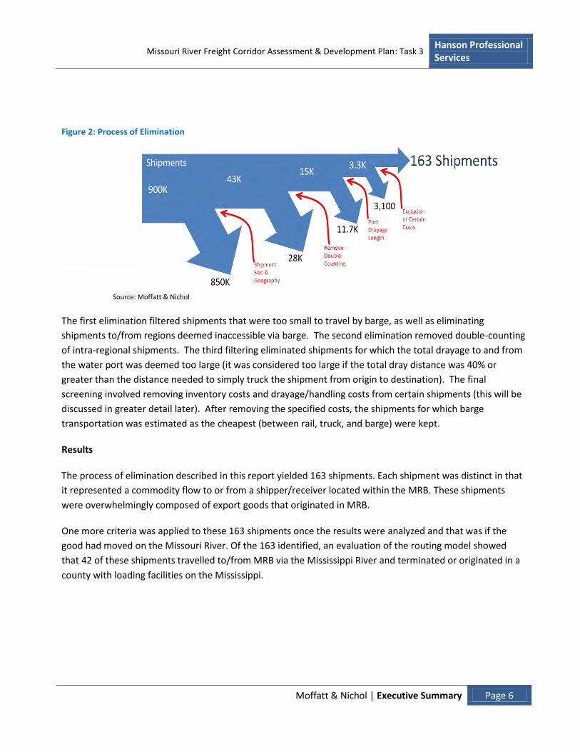
Figure 2: Process of Elimination
Source: Moffatt & Nichol
The first elimination filtered shipments that were too small to travel by barge, as well as eliminating
shipments to/from regions deemed inaccessible via barge. The second elimination removed double-counting
of intra-regional shipments. The third filtering eliminated shipments for which the total drayage to and from
the water port was deemed too large (it was considered too large if the total dray distance was 40% or
greater than the distance needed to simply truck the shipment from origin to destination). The final
screening involved removing inventory costs and drayage/handling costs from certain shipments (this will be
discussed in greater detail later). After removing the specified costs, the shipments for which barge
transportation was estimated as the cheapest (between rail, truck, and barge) were kept.
Results
The process of elimination described in this report yielded 163 shipments. Each shipment was distinct in that
it represented a commodity flow to or from a shipper/receiver located within the MRB. These shipments
were overwhelmingly composed of export goods that originated in MRB.
One more criteria was applied to these 163 shipments once the results were analyzed and that was if the
good had moved on the Missouri River. Of the 163 identified, an evaluation of the routing model showed
that 42 of these shipments travelled to/from MRB via the Mississippi River and terminated or originated in a
county with loading facilities on the Mississippi.
Missouri River Freight Corridor Assessment & Development Plan: Task 3 Hanson Professional Services
Moffatt & Nichol | Executive Summary Page 7
Figure 3 illustrates the type of shipments that make-up the 59 million tonnes (121 shipments) that moved via
the Missouri River. Movements with an origin and destination within the MRB (Intra-regional movements)
and movements with an origin outside of the MRB but a destination within the MRB (Inbound movements)
account for a small share of the potential volumes. On the other hand, movements with an origin in the
MRB, but a destination outside of it (Outbound movements) make up the majority of the potential tonnage.

Missouri River Freight Corridor Assessment & Development Plan: Task 3 Hanson Professional Services
Moffatt & Nichol | Executive Summary Page 8
Figure 3: Potential Barge Movement by Shipment Type (% of Total Tonnage)
Source: Moffatt & Nichol
Figure 4 illustrates the potential shipments broken down by commodity. The majority of the volumes are
made up of commodities which are produced/consumed in large quantities and tend to be shipped on
irregular schedules due to their high dwell times. These include Other Ag Products (which are primarily
soybeans), cereal grains, and coal and petroleum products n.e.c. The absence of manufactured goods –
excluding equipment - is due largely to the need for these goods to be shipped on a regular basis, thus their
shipment sizes tended to be smaller than bulk goods because the annual shipment quantities were shipped
on a weekly basis. Two other factors further limited the suitability of barge as a means of transporting
manufactured goods to the region. The first is that most manufactured goods travel in a West-East direction
while the Missouri River is most suited to commodities moving North-South. The other is that manufactured
goods have the cost of labor imbedded in their purchase price, and thus are more sensitive to inventory
carrying costs.
Figure 4: Potential Barge Shipments by Commodity (% of Total Tonnage)
Source: Moffatt & Nichol
Outbound75%
Intra-regional24%
Inbound1%
Total Potential Tonnage = 59 million tonnes
Other ag prods.46%
Cereal grains29%
Coal-n.e.c. & Petro goods
n.ec.11%
Nonmetal mineral
products3%
Other11%
Total Potential Tonnage = 59 million tonnes

Hanson Professional Services
Missouri River Freight Corridor Assessment & Development Plan: Task 3
Moffatt & Nichol | Conclusions Page 9
One other factor that influence the number of potential barge shipments identified through the elimination process was the geographical location of the shipper within MRB.
Figure 5 graphically illustrates the origin, destination and shipping route of the shipments. Within MRB, the origin and destination counties from/to which shipments are made/received (represented in brown and yellow respectively) are located adjacent to or in very close proximity to the Missouri River. This highlights the impact of the additional transportation cost required to reach inland destinations which increases the cost of barging vs. other modes of transportation. For inter-regional shipments, the destination of Outbound shipments from MRB are shown in blue while the origin of Inbound shipments to MRB are shown in pink.
Figure 5: Heat Map of Potential Shipments
Source: Moffatt & Nichol
Missouri River Freight Corridor Assessment & Development Plan: Task 3 Hanson Professional Services
Moffatt & Nichol | Executive Summary Page 10
Conclusions
Moffatt & Nichol identified 121 shipments that could potentially be routed for at least part of their supply
chain to barge on the Missouri River.
Three characteristics regarding potential barge movements emerged from the analysis:
The shipper or receiver should be located on the water. The cost and time associated with
drayage/handling between a port and an off water facility tends to make barge less affordable.
Shipment sizes must be sufficiently large in order to utilize barge capacity (for bulk shipments).
Because barge is a much slower mode of transport, the shipment must be capable of absorbing
inventory carrying costs accrued en route.
Missouri River Freight Corridor Assessment & Development Plan: Task 3 Hanson Professional Services
Moffatt & Nichol | Model Flow Page 11
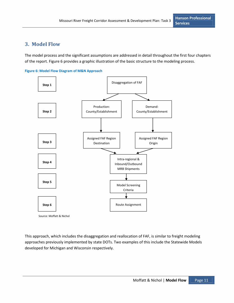
3. Model Flow
The model process and the significant assumptions are addressed in detail throughout the first four chapters
of the report. Figure 6 provides a graphic illustration of the basic structure to the modeling process.
Figure 6: Model Flow Diagram of M&N Approach
Source: Moffatt & Nichol
This approach, which includes the disaggregation and reallocation of FAF, is similar to freight modeling
approaches previously implemented by state DOTs. Two examples of this include the Statewide Models
developed for Michigan and Wisconsin respectively.
Step 1
Production:
County/Establishment
Demand:
County/Establishment Step 2
Assigned FAF Region
Destination
Assigned FAF Region
Origin Step 3
Model Screening
Criteria
Step 4
Route Assignment
Intra-regional &
Inbound/Outbound
MRB Shipments
Disaggregation of FAF
Step 6
Step 5

Missouri River Freight Corridor Assessment & Development Plan: Task 3 Hanson Professional Services
Moffatt & Nichol | Model Flow Page 12
Michigan Statewide Truck Model (1998 used 1997 CFS data)
Attempts to equate value of goods shipments per 1000 employees of the generating industry
Trip generation and destination was carried out at the Commodity Analysis Zone (CAZ) and
allocated to the counties using the employment by industry
Destination choice model was used to allocate trip origins. This model was mathematically
equivalent to a simple constrained gravity model
The number of truck loads was determined by dividing the total shipment tonnage by the
average freight load of a truck
Wisconsin Statewide Model (2007 Transearch Data)
Total production, in tons per employee by industry, is calculated at the state level
Production is then allocated to the county level using the CBP data, by taking the county share of
total employment
Additional disaggregation of production to the Commodity Analysis Zone (CAZ) within each
county is done using the population at that level
State level input-output accounts were used to derive attractions for business and households.
Allocation to the country level was conducted using the share of consuming industries
designated in the CBP data.
A gravity model was used to distribute trips into three classifications: internal, internal-external,
and external internal.

Missouri River Freight Corridor Assessment & Development Plan: Task 3 Hanson Professional Services
Moffatt & Nichol | Use of FAF Data Page 13
4. Use of FAF Data
In the simulation of commodity flows through the MRB region, Moffatt & Nichol uses the FAF3 data as the
control total. This data set has been disaggregated, and the commodity flow totals within the MRB study
region have been reallocated to the county level from the larger FAF regions.
The FAF data has been widely accepted and incorporated into other freight movement analysis. Two
examples include, “The Delaware Valley Regional Planning Commission developed tables from the FAF2
origin-destination database to illustrate domestic and foreign freight flows into the Philadelphia region,” and
“The FAF2 origin-destination database was used to develop estimates of internal-external and through truck
trips for a truck model of the San Diego region” (Donnelly).
FAF 3 is the third version of the FAF database, first developed in 1997-1999. “FAF3 is a Federal Highway
Administration (FHWA) funded and managed data and analysis program that provides estimates of the total
volumes of freight moved into, out of and within the United States, between individual states, major
metropolitan areas, sub-state regions, and major international gateways” (Southworth).
Working with a base year of 2007, FAF3 uses multiple sources of data including the 2007 Commodity Flow
Survey, the Surface Transportation Board’s public use railcar waybills, the US Army Corps of Engineers
Waterborne commerce dataset and also calls upon other datasets, such as PIERS data.
The main data products of FAF are:
• “A set of annual freight flow matrices, reported in annual tonnages and annual dollar value of goods
transported, for calendar year 2007 for the United States,
• Based on these base year flow estimates, a set of forecast year freight flow matrices, projected out
to calendar year 2040,
• A set of annual freight tonnage and vehicle/vessel movement volumes assigned to specific links and
routes over the United States multimodal truck-rail-waterways transportation network, based on
these base year 2007 and forecast year 2040 flow estimates.”
“Based on these estimated freight flows and their network assignments, a set of annual freight tonnage,
dollar value, and ton-mileage statistics, broken down by mode of transport and commodity class are also
developed” (Southworth).

Missouri River Freight Corridor Assessment & Development Plan: Task 3 Hanson Professional Services
Moffatt & Nichol | Methodology Page 14
5. Methodology
5.1. Disaggregation of FAF
The first step in generating firm level routings is to disaggregate the FAF shipment information from SCTG to
BEA-IO codes. The disaggregation of FAF data from SCTG to BEA-IO codes leads to higher level granularity in
the analysis. At this higher level each commodity is treated differently and commodity specific results are
created. The disaggregated FAF shipments are used to control commodity production of the economic
simulator to create FAF controlled, firm level Origination/Attraction information.
This ability to analyze commodity specific routings is necessary to study the impact of different scenarios on
individual products in a manner aimed at understanding how different markets are affected with different
policies.
The flow of disaggregating FAF data to estimate firm level production/origination information is illustrated in
Figure 7.
Figure 7: Flow Diagram FAF Disaggregation
Source: Moffatt & Nichol

Missouri River Freight Corridor Assessment & Development Plan: Task 3 Hanson Professional Services
Moffatt & Nichol | Methodology Page 15
5.2. Identifying Production/Attraction at the County and Establishment Level
The first step in simulating the economy is to create a comprehensive map of local businesses. By so doing, a
geographic framework is established in order to identify sources of production and attraction for the
commodity flows within the study region. The base data comes from the County Business Patterns (CBP)
released by the US Census Bureaui. CBP provides annual geographic and industry data for U.S. business
establishments at the county and industry level.
At the county level this data is often suppressed to avoid disclosure or for not meeting publication standards.
The extent of suppression decreases at higher geographic levels where the data is more aggregated.
Therefore in order to estimate suppressed county level data a hierarchical approach using State and National
level data is used; as identified in Figure 8. At the national level for each NAICS code, the average number of
employees for each employee size bracket is calculatedii. At the state level, the average number of
employees for each bracket size is calculated for available data; if the data is suppressed the national average
is used as the estimator. By following the same logic, detailed county level data is estimated with a very good
margin of error, as compared to the aggregate level of employment per county as reported in CBPiii.
Figure 8: Top-Down Hierarchy to Estimate Suppressed County Data
Source: Moffatt & Nichol
Table 1 provides an example of the CBP employment data at the county level by NAICS. The example is for
Dubuque County (061), in Iowa (19). The NAICS codes are furniture and home goods retailers.
Table 1: Example of CBP Employment Data
FIPS Empty Number of Number of Establishments by Employee Size Bracket
State County NAICS Flag Emp. Estab. 1-4 5-9 10-19 20-49 50-99 100-249 250-499 500-999 1000+
19 061 442110 95 17 8 6 3 0 0 0 0 0 0
19 061 442210 46 7 2 4 1 0 0 0 0 0 0
19 061 442291 A 0 1 1 0 0 0 0 0 0 0 0
19 061 442299 100 5 2 0 2 0 1 0 0 0 0
19 061 443111 A 0 4 2 2 0 0 0 0 0 0 0
Source: US Census Bureau; Moffatt & Nichol

Missouri River Freight Corridor Assessment & Development Plan: Task 3 Hanson Professional Services
Moffatt & Nichol | Methodology Page 16
Production
Detailed firm level production by commodity is needed because firms of different sizes have different
shipping behavior.
As with the previous estimation where in certain instances data was suppressed at the county level, Table 2
shows how a hierarchical approach using data from the Economic Censusiv (EC) was used to estimate the
production per employee at the county level. If the information is available at the county level, county level
estimation will be used (NAICS = 444220, 445110). If the county level data is suppressed, and state level data
is available, state level estimation is used (NAICS = 445120). Otherwise national level productivity estimation
is used (NAICS = 445210, 445220).
Table 2: Example of Economic Census Production by Geographic Hierarchy by NAICS
NAICS6 Production per Employee ($1000s)
State County NAICS County Level Productivity
State Level Productivity
National Level Productivity
01 003 444220 225.65 235.65 217.77
01 003 445110 178.48 151.46 191.67
01 003 445120 241.75 175.79
01 003 445210 147.41
01 003 445220 179.82 Source: US Census Bureau; Moffatt & Nichol
The total value of shipment of an individual firm is calculated by combining NAICS6-County level production
per employee with NAICS6-Countly level firm size information.
It should be noted that CBP does not include information on agriculture. Therefore, Moffatt & Nichol used
data provided in the Census of Agriculture, conducted by the USDA, to estimate county level production.
Figure 9 presents the production value by BEA-IO (given in descriptive title) for FAF regions within MRB.

Hanson Professional Services
Missouri River Freight Corridor Assessment & Development Plan: Task 3
Moffatt & Nichol | Methodology Page 17
Figure 9: Agriculture Production by BEA-IO Code
Source: US Census Bureau; Bureau of Economic Analysis; Moffatt & Nichol
Using Production Requirements to Estimate Levels of Attraction
Having established the county level production profiles described above, the next step in allocating FAF commodity flows to the county level was to determine the points of commodity attraction. These attraction locations are determined by the level of intermediate inputs consumed during production and/or the level of final goods sold. There are four basic types of attraction that occur in regular frequency:
intermediate demand via wholesaler, intermediate demand directly sourced, final good demand via wholesaler, and final good via warehousing
Moffatt & Nichol used the two following supply chain rules to frame the analysis. If an intermediate (e.g. a wholesaler) is used, commodity flows into the region (attraction) are modeled coming into the region to the location of the intermediate. Additionally, the movement from an intermediate to final demand is not
0
2000
4000
6000
8000
10000
12000
14000
16000
18000
20000
190 201 209 291 292 299 310 460
Valu
e ($
Mill
ions
)
MRB FAF Regions
Forest nurseries, forest products, and timber tractsAnimal production, except cattle and poultry and eggsPoultry and egg production
Cattle ranching and farming
Dairy cattle and milk production
All other crop farming
Cotton farming
Tobacco farming
Fruit farming
Vegetable and melon farming
Grain farming
Oilseed farming

Missouri River Freight Corridor Assessment & Development Plan: Task 3 Hanson Professional Services
Moffatt & Nichol | Methodology Page 18
modeled. The process used to estimate attraction for intermediate and final (retail) goods is described
below.
Intermediate Demand
The 2002 Benchmark IOv tables are used to determine the demand for intermediate production inputs for all
industries. These tables show the commodities and the value added components that an industry requires to
create a unit of output. Moffatt & Nichol applied these direct requirement coefficients to the estimated firm
level revenues aggregated from NAICS6 to the BEA-IO codes to estimate the input requirements per NAICS6.
As an example, Figure 10 provides the breakdown of the direct commodity requirements needed by the
Oilseed Farming industry (BEA-IO 1111AO).
Figure 10: Direct Commodity Requirements for Oilseed Farming
Source: US Census Bureau; Bureau of Economic Analysis; Moffatt & Nichol
Special Case: Construction is assumed to be the value of all revenue earned by construction firms in the
respective counties.
Gross operating surplus
Real estate
Oilseed farming
Support activities for agriculture and forestry
Monetary authorities and depository credit intermediation
Compensation of employees
Pesticide and other agricultural chemical manufacturing
Petroleum refineries
other

Missouri River Freight Corridor Assessment & Development Plan: Task 3 Hanson Professional Services
Moffatt & Nichol | Methodology Page 19
Similar intermediate input profiles, such as that presented in Figure 10, are established for each industry. The
respective compositions of these profiles are later used to study how different firms satisfy their
intermediate demand. The locations of intermediate input demand become the sources of attraction within
the model.
Within the modeling process, several sub-rules are made to help determine likely shipment size coming into
the region. These rules are applied to reflect the existing supply chain structure. These are listed below and
summarized in Table 3:
1. Firms with less than 100 employees are assumed to purchase all inputs via wholesalers
2. Firms with greater than 100 employees but less than 500 are assumed to source inputs
with value at or above 10% of revenues directly from a manufacturer. Inputs valued at
less than 10% of revenues are assumed to be purchased via wholesaler.
3. Firms with more than 500 employees purchase all inputs with value at or greater than
5% directly from a manufacturer. Inputs less than 5% are sourced via wholesaler.
Table 3: Sub-Rules Applied to Modelling of Intermediate Attraction
Firms Size
Less than 100 Between 100 and 500 More than 500
Inp
ut
Rat
io Less than 5% Wholesaler Wholesaler Wholesaler
Between 5% and 10% Wholesaler Wholesaler Direct
More than 10% Wholesaler Direct Direct
Source: Moffatt & Nichol
While smaller firms with less than 100 employees may not individually generate the demand volume which
would require a barge movement, the market rules identified in Table 3 dictate that their demand be
handled via a wholesaler. It is this consolidation which allows for more barge-eligible demand and a realistic
approach toward modeling the market.
Applying these rules to the total of firms in the MRB generates the market structure illustrated in Figure 11.

Missouri River Freight Corridor Assessment & Development Plan: Task 3 Hanson Professional Services
Moffatt & Nichol | Methodology Page 20
Figure 11: Total Firm Revenue by Number of Employees
Source: US Census Bureau; Bureau of Economic Analysis; Moffatt & Nichol
Retail Demand
Retail demand is the other source of attraction to the region and is estimated on information published in
Table EC07443 of the Economic Census. This table contains data on the number of establishments and their
total salesvi. Information from table EC07443 is used to allocate demand for different product lines from the
simulated economy. This is done by reducing the total estimated retail establishment revenue and calculating
the demand for different product lines as a percentage of the reduced revenue of the retail establishment.
Figure 12 provides an example of the composition of an electronic store’s sales.
Figure 12: Percentage of Total Revenue for Radio, Television, and Other Electronics Stores (BEA-IO 443112)
Source: US Census Bureau; Bureau of Economic Analysis; Moffatt & Nichol
Less than 100
Between 100 and 500
More than 500
Computer & peripheral equipment
Televisions & related parts & accessories
Telephones, including cellular phones
Audio equipment, components, parts & accessories
Prepackaged computer software, including software downloads
Other
Missouri River Freight Corridor Assessment & Development Plan: Task 3 Hanson Professional Services
Moffatt & Nichol | Methodology Page 21
As previously described for intermediate demand, it is necessary to make rules related to market structure.
These rules determine the configuration of the supply chain. Retailers are classified by size based on whether
they purchase goods directly from the producer or via a wholesaler.
Retail establishments with fewer than 250 employees are assumed to purchase goods via a
wholesaler.
Retail establishments with over 250 employees source goods directly and their goods are
stored at a warehouse until sorted and moved to the final retail destination.
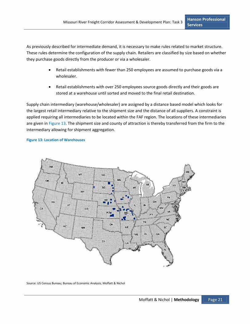
Supply chain intermediary (warehouse/wholesaler) are assigned by a distance based model which looks for
the largest retail intermediary relative to the shipment size and the distance of all suppliers. A constraint is
applied requiring all intermediaries to be located within the FAF region. The locations of these intermediaries
are given in Figure 13. The shipment size and county of attraction is thereby transferred from the firm to the
intermediary allowing for shipment aggregation.
Figure 13: Location of Warehouses
Source: US Census Bureau; Bureau of Economic Analysis; Moffatt & Nichol
Missouri River Freight Corridor Assessment & Development Plan: Task 3 Hanson Professional Services
Moffatt & Nichol | Methodology Page 22
5.3. Allocation of FAF to County Level
Following the identification of sources of production and attraction, the next step was to allocate the
commodity flow values reported in FAF to the county level. As a result of differing geographies (county vs.
FAF region) Moffatt & Nichol used a simple distribution algorithm to assist in this process, based on the
assumption that an inverse relationship exists between establishment size and distance of trade; i.e. larger
firms tend to serve distant markets while small firms serve local markets. This assumption has been well
established and documented in previous analysis, most recently by Holmes and Thomas (2010) who in their
study conclude:
“Export destinations tend to be further than domestic destinations, and large plants tend to ship
further distances even to domestic locations as compared to small plants.”
Additionally, referring to the work of Melitz (2003) and Stevens (2010):
“…that even within a narrowly defined industries, small plants tend to perform retail-like functions
that are difficult to trade (e.g., custom work), compared with large plants in the same industry”...
”that small plants tend to be geographically diffuse and follow the distribution of population, while
large plants tend to be geographically concentrated, is consistent with the shipment distance findings
reported here. As the small plants follow the distribution of population, they can meet demand by
serving local customers, just like retail stores do. As the large plants may be concentrated in just a
few locations, goods must be shipped to distant locations that have no source of local supply.”
Based on this assumption, Moffatt & Nichol used the algorithm to assign the largest establishments in the
FAF region and BEA-IO category volumes from the furthest origination/destination .The algorithm allocates
between these two until all establishments are assigned to a FAF origin/destination.
Moffatt & Nichol used the value of revenue by NAICS, as reported in the CBP, as the measure of relative
production and attraction at the county level. The value of revenue was used to help explain the varying
trade routes by which high and low value commodities travel designated in the FAF data. Through the
decomposition of SCTG to BEA-IO codes, Moffatt & Nichol is able to reconstruct a value per ton of shipment
of the SCTG codes, and assign the lower value commodities to the lower value trade routes, and vice versa.
The cumulative value of revenue was controlled to the FAF total value of trade flow to ensure 100%
allocation.

Missouri River Freight Corridor Assessment & Development Plan: Task 3 Hanson Professional Services
Moffatt & Nichol | Methodology Page 23
Table 4 offers a sample output of the allocation algorithm. It provides the domestic originations and
destinations along with the company size and the value and volume for different commodity shipments.
Three different types of pairings are indicted:
Intra-regional pairing has an origin and destination within the MRB region;
Outbound pairing has an origin in the MRB region but a destination outside the MRB region and
Inbound pairing has an origin outside the MRB region but a destination within the MRB region
For computational purposes it was advantageous to pair the county-to-FAF Region for Outbound pairings and
the FAF Region-to-County for Inbound pairings. All Intra-regional MRB pairs are identified on a County-to-
County basis.
Table 4: Sample Output of the Allocation Algorithm
Type
Origin FIPS
(County)
Domestic Origin (FAF
Region)
Domestic Destination
(FAF Region)
Destination FIPS
(County) Company
Size BEA-IO Code SCTG Milevii Value (mls)
Volume (KT)
Inbound 560 209 20173 1-4 212100 15 750 206.77 27965.34
Inbound 560 292 29071 1-4 212100 15 1115 57.61 7761.61
Inbound 560 292 29510 5-9 212100 15 1115 7.80 1050.46
Outbound 29186 299 229 100-249 212310 12 604 0.16 38.69
Outbound 29186 299 229 100-249 212310 12 604 0.11 27.48
Outbound 29091 299 471 20-49 212310 12 363 0.21 52.87
Intra- regional 20177 209 209 20177 1-4 212320 11 12 0.01 1.84
Intra- regional 20055 209 209 20093 1-4 212320 11 24 3.63 581.57
Intra- regional 20201 209 209 20027 1-4 212320 11 32 0.37 58.91
Source: Federal Highway Administration; US Census Bureau; Bureau of Economic Analysis; Moffatt & Nichol
These pairings are then used as inputs into the routing model which will estimate the least cost routes
between different origin and destination parings. Each row of the table acts as an individual customer to the
system. The model will measure the effectiveness of different scenarios by solving it for the least cost route
of these individual customers.

Missouri River Freight Corridor Assessment & Development Plan: Task 3 Hanson Professional Services
Moffatt & Nichol | Methodology Page 24
It should be noted that within the sample data, of the firms which ship the same commodity (212310) from
the same domestic origin (FAF 299), it is the large firm which ships the furthest distance; as designated by the
allocation algorithm.
Figure 14 is the histogram of total shipment volume based on distance shipped. As illustrated, most of the
Intra-regional volumes travel less than 200 miles. By comparison, the Outbound and Inbound volumes travel
distances tend to be greater.
Figure 14: Histogram of Shipment by Distance by Trade Pairing
Source: Moffatt & Nichol
0 200 400 600 800 1000 1200 1400 16000
10
20
30
40
50
60
70
80
90Distance-Volume
Miles
Perc
enta
ge o
f T
ota
l
Intra-Regional
Outbound
Inbound

Missouri River Freight Corridor Assessment & Development Plan: Task 3 Hanson Professional Services
Moffatt & Nichol | Process of Elimination Page 25
6. Process of Elimination
The process of elimination explains how the original data was reduced to a manageable size to be used in
model without the loss of the applicability of the result.
Figure 15: Process of Elimination
Source: Moffatt & Nichol
As shown in Figure 6 MRB shipments are initially classified into two categories of shipments, those
originating from MRB and those attracted to MRB. The allocation algorithm creates an extensive list of
potential routing O&D pairs with approximately 90,000 routes identified as originations and 800,000 as
attractions.
Figure 16 and Figure 17 highlight an import point, namely that a low number of large-volume shipments
account for significantly more of the total tonnage as compared to the small share held by a high number of
small-volume shipments.
The scale of the horizontal axis is scaled into “bins” which are representative of the different transportation
mode types load capacities: 0-27 (truck), 28 – 104 (rail), 105 – 1,360 (barge), 1,361+ (multiple barges).
Figure 16 illustrates the number of routes based on their shipment size. The horizontal axis shows the route
volume identified and the vertical axis shows the share of routings within the volume range from total
number of routings. The small-volume shipments account for the most share by count.
Figure 17 illustrates the volume of the routes based on their shipment size. This shows that despite their
significant share of total number of routes, low volume routes don’t have a significant contribution in the
movement of commodities. Shipments of 0 to 27 tonnes account for about 30% of Origination and more than
70% of Attraction; however their share in total volumes is insignificant.

Hanson Professional Services
Missouri River Freight Corridor Assessment & Development Plan: Task 3
Moffatt & Nichol | Process of Elimination Page 26
Per
cent
age
of T
otal
Vol
ume
Car
ried
on th
e R
oute
P
erce
ntag
e of
Tot
al N
umbe
r or
Rou
tes
If used directly in the final route choice model, this original data set would impose a great computational burden; therefore the first exclusionary criteria (EC) were applied to the model.
The scale of the horizontal axis is scaled into “bins” which are representative of the different transportation mode types load capacities: 0-27 (truck), 28 – 104 (rail), 105 – 1,360 (barge), 1,361+ (multiple barges).
Figure 16: Route count histogram by shipment size
0.8
0.7
Count histogram Origination Attraction
0.6
0.5
0.4
0.3
0.2
0.1
0
0-27 28-104 105-1360 1361-... Route-Volume (Tonnes)
Source: Moffatt & Nichol
Figure 17: Route volume histogram by shipment size
1
0.9
Origination Attraction
Volume histogram
0.8
0.7
0.6
0.5
0.4
0.3
0.2
0.1
0
0-27 28-104 105-1360 1361-... Route-Volume (Tonnes)
Source: Moffatt & Nichol

Hanson Professional Services
Missouri River Freight Corridor Assessment & Development Plan: Task 3
Moffatt & Nichol | Process of Elimination Page 27
Elimination Criteria-A
The routing model is focused on large-volume shipments which are more likely to be routed by barge. Therefore, the first screening filtered shipments which would be too small to ship by barge as determined by a combination of the frequency at which they were shipped and the stowage factors of the commodities being modeled.
The second screening applied at this stage included the elimination of shipments to and from FAF regions which are inaccessible via barge. Figure 18 shows a map of the FAF regions considered accessible and those that were not.
Figure 18: Map of Accessible FAF Regions
Source: Moffatt & Nichol

Missouri River Freight Corridor Assessment & Development Plan: Task 3 Hanson Professional Services
Moffatt & Nichol | Process of Elimination Page 28
By applying these two filters, the total number of routings would decrease to about 13,000 from the initial
90,000 for origination, and to 30,000 from the initial 800,000 for attractions. This significant reduction in the
number of routings is accomplished without compromising the applicability of the outcome as shown in
Figure 19.
The chart on the left shows that by count, the total number of routes has been isolated to the larger
shipments, while the smaller shipments have been eliminated altogether. However, in terms of tonnage, the
vast majority of the volume has remained in the largest shipments as shown in the chart on the right,
signaling that the structure of the original data set has been maintained throughout this first elimination.
Figure 19: Count and Volume of Second Data Set
Source: Moffatt & Nichol
Elimination Criteria-B
The next layer of screening took the filtered origination and attraction tables and combined them together to
remove the double counting of routes which originate in and are destined to locations in MRB. These became
the Intra-regional shipments.
Additionally, the warehousing and wholesaling rules explained in section 5.2 were applied to consolidate
small shipments into larger ones. The resulting third data set had 14,763 routings with the following
composition for route counts and volume:
0-27 28-104 105-1360 1361-...0
0.1
0.2
0.3
0.4
0.5
0.6
0.7
0.8
0.9
1Count histogram (filtered by direction and water max load)
Route-Volume (Tonnes)
Perc
enta
ge o
f T
ota
l N
um
ber
or
Route
s
Origination
Attraction
0-27 28-104 105-1360 1361-...0
0.1
0.2
0.3
0.4
0.5
0.6
0.7
0.8
0.9
1Volume histogram (filtered by direction and water max load)
Route-Volume (Tonnes)
Perc
enta
ge o
f T
ota
l V
olu
me C
arr
ied o
n t
he R
oute
Origination
Attraction

Missouri River Freight Corridor Assessment & Development Plan: Task 3 Hanson Professional Services
Moffatt & Nichol | Process of Elimination Page 29
Figure 20: Count and Volume of Third Data Set
Source: Moffatt & Nichol
Elimination Criteria-C
The next step of screening was the elimination of O&D pairings for which total port drayage distances were
greater than 40% of the direct trucking distance. These pairs were eliminated so that drayage associated
with a barge move would not be adversely increased by long drayage from counties in the far corners of the
study area routed to the Missouri River.
The resulting data set had 3,382 routings with the following composition for route counts and volume:
Figure 21: Count and Volume of Fourth Data Set
Source: Moffatt & Nichol
0-27 28-104 105-1360 1361-...0
0.1
0.2
0.3
0.4
0.5
0.6
0.7
0.8
0.9Route-count histogram (Combined Origination and Attraction)
Route-Volume (Tonnes)
Perc
enta
ge o
f T
ota
l N
um
ber
or
Route
s
0-27 28-104 105-1360 1361-...0
0.1
0.2
0.3
0.4
0.5
0.6
0.7
0.8
0.9
1Volume histogram (Combined Origination and Attraction)
Route-Volume (Tonnes)
Perc
enta
ge o
f T
ota
l V
olu
me C
arr
ied o
n t
he R
oute
0-27 28-104 105-1360 1361-...0
0.1
0.2
0.3
0.4
0.5
0.6
0.7
0.8
0.9Route-count histogram (Long Dray Cut Down)
Route-Volume (Tonnes)
Perc
enta
ge o
f T
ota
l N
um
ber
or
Route
s
0-27 28-104 105-1360 1361-...0
0.1
0.2
0.3
0.4
0.5
0.6
0.7
0.8
0.9
1Volume histogram (Long Dray Cut Down)
Route-Volume (Tonnes)
Perc
enta
ge o
f T
ota
l V
olu
me C
arr
ied o
n t
he R
oute
Missouri River Freight Corridor Assessment & Development Plan: Task 3 Hanson Professional Services
Moffatt & Nichol | Process of Elimination Page 30
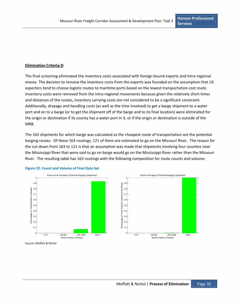
Elimination Criteria-D
The final screening eliminated the inventory costs associated with foreign bound exports and intra-regional
moves. The decision to remove the inventory costs from the exports was founded on the assumption that US
exporters tend to choose logistic routes to maritime ports based on the lowest transportation cost route.
Inventory costs were removed from the Intra-regional movements because given the relatively short times
and distances of the routes, inventory carrying costs are not considered to be a significant constraint.
Additionally, drayage and handling costs (as well as the time involved) to get a barge shipment to a water
port and on to a barge (or to get the shipment off of the barge and to its final location) were eliminated for
the origin or destination if its county has a water port in it, or if the origin or destination is outside of the
MRB.
The 163 shipments for which barge was calculated as the cheapest route of transportation are the potential
barging routes. Of these 163 routings, 121 of them are estimated to go on the Missouri River. The reason for
the cut-down from 163 to 121 is that an assumption was made that shipments involving four counties near
the Mississippi River that were said to go on barge would go on the Mississippi River rather than the Missouri
River. The resulting table has 163 routings with the following composition for route counts and volume:
Figure 22: Count and Volume of Final Data Set
Source: Moffatt & Nichol
0-27 28-104 105-1360 1361-...0
0.1
0.2
0.3
0.4
0.5
0.6
0.7
0.8
0.9
1Route-count histogram (Potential Barging Shipments)
Route-Volume (Tonnes)
Perc
enta
ge o
f T
ota
l N
um
ber
or
Route
s
0-27 28-104 105-1360 1361-...0
0.1
0.2
0.3
0.4
0.5
0.6
0.7
0.8
0.9
1Volume histogram (Potential Barging Shipments)
Route-Volume (Tonnes)
Perc
enta
ge o
f T
ota
l V
olu
me C
arr
ied o
n t
he R
oute

Missouri River Freight Corridor Assessment & Development Plan: Task 3 Hanson Professional Services
Moffatt & Nichol | Mode Choice Simulation Page 31
7. Mode Choice Simulation
Barged Commodities and Their Relation to Logistics Costs
Two overriding characteristics, namely large volume and low value, generally allow for a given commodity to
be shipped by barge, as evidenced by the current mix of commodities illustrated in Figure 23.
In 2008 approximately 589 million tons of cargo was transported on the US’s intercoastal waterways, of
which coal was the largest volume accounting for 31% of the total, followed by petroleum (25%) and crude
materials including gravel and sand (18%). Agriculture products, primarily grains and soybeans, chemicals and
manufactured goods also account for a significant share of the total weight.
These goods are typically shipped in very large quantities in order to capture the lower transportation costs
associated with economies-of-scale. Given the large shipment size and the slower form of transportation,
the inventory carrying costs associated with these bulk commodities are generally lower by comparison to
that of other high value commodities, particularly consumer related goods.
Figure 23: 2008 Intercoastal Waterway Volumes by Commodity Share
Source: US Army Corps of Engineers Waterborne Commerce Data
Coal31%
Petroleum25%
Crude Materials18%
Foods & Farm12%
Chemicals8%
Manufactured Goods
4%
Manufactured Equipment
2%
Other0%
Missouri River Freight Corridor Assessment & Development Plan: Task 3 Hanson Professional Services
Moffatt & Nichol | Mode Choice Simulation Page 32
Barge Capacity Relative to Truck and Rail
As compared to truck or rail, barge transport exhibits strong economies of scale. Shipping large volumes in
bulk reduces the fixed cost per unit of commodity.
In part this is due to the load carrying capacity of a barge, which is much greater than that of either truck
and/or rail. In order to utilize this capacity efficiently, thus lowering the average cost of transportation per
ton, significant volumes of material must be available to fill the barge.
The average capacity of a river barge is approximately 1,500 tons, as compared to the average 25 tons per
truck and 100 tons per rail car; suggesting that every barge load can carry the equivalent of 60 trucks or 15
rail cars. The comparison is more dramatic once the average size of a barge tow is considered.
Barge tows typically consist of 15 barges (5 long × 3 abreast) on sections of the Mississippi River with locks,
and can increase to 30 or 40 barges on sections where there are no locks. If the same equivalent described
above is applied to the smaller tow size, this suggests that 900 truck loads and/or 225 rail car loads can be
accommodated by a single 15-barge tow.
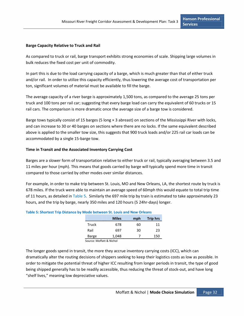
Time in Transit and the Associated Inventory Carrying Cost
Barges are a slower form of transportation relative to either truck or rail, typically averaging between 3.5 and
11 miles per hour (mph). This means that goods carried by barge will typically spend more time in transit
compared to those carried by other modes over similar distances.
For example, in order to make trip between St. Louis, MO and New Orleans, LA, the shortest route by truck is
678 miles. If the truck were able to maintain an average speed of 60mph this would equate to total trip time
of 11 hours, as detailed in Table 5. Similarly the 697 mile trip by train is estimated to take approximately 23
hours, and the trip by barge, nearly 350 miles and 120 hours (5 24hr-days) longer.
Table 5: Shortest Trip Distance by Mode between St. Louis and New Orleans
Miles mph Trip hrs
Truck 678 60 11
Rail 697 30 23
Barge 1,048 7 150 Source: Moffatt & Nichol
The longer goods spend in transit, the more they accrue inventory carrying costs (ICC), which can
dramatically alter the routing decisions of shippers seeking to keep their logistics costs as low as possible. In
order to mitigate the potential threat of higher ICC resulting from longer periods in transit, the type of good
being shipped generally has to be readily accessible, thus reducing the threat of stock-out, and have long
“shelf lives,” meaning low depreciative values.

Missouri River Freight Corridor Assessment & Development Plan: Task 3 Hanson Professional Services
Moffatt & Nichol | Mode Choice Simulation Page 33
Therefore, the most common commodities which meet these criteria are typically the large volumes of bulk
goods, including mined/quarried material and agriculture products.
Additionally, many of the end users of the bulk materials shipped by barge, including utilities, are located on
or have receiving facilities in close proximity to the inland waterway.
Proximity: In the Context of Container & Break Bulk Cargos
The use of barge for moving containerized commodities generally remains limited to inter-port redistribution
services, such as that linking the Ports of Baltimore, Philadelphia, and NY/NJ, and the RO/RO barge services
between mainland US ports and the Caribbean Islands and Alaska. Factors that limit the use of barges to
carry containers include:
Slow speed of barge impacting inventory costs
High load on/load off terminal handling costs
The extended time required to accumulate a barge load of containers, particularly as compared to
trucks
Furthermore, the inland infrastructure which has supported the rapid growth of container trade in the US,
namely an international and regional network of inland ports, intermodal yards, and distribution centers
strategically located near or adjacent to primary connecting road and rail networks is not geared toward the
inland waterway structure.

Missouri River Freight Corridor Assessment & Development Plan: Task 3 Hanson Professional Services
Moffatt & Nichol | Mode Choice Simulation Page 34
7.1. Routing Simulation Inputs
In order to calculate the least cost route/mode of shipping, many different parameters have to be estimated.
These parameters can either be associated with costs or with time (which is then converted in to inventory
carrying cost). They can also be broken down as relating to either “links” or “nodes”. Links are defined as
surface pathways over which goods are transported (roads, rails, or waterways) while nodes are connecting
points (terminals) where goods are lifted off or on, stored, or manipulated.
Link Costs
Truck: Two different trucking rates were used, one for drayage (determined to be trucking of 100 miles and
under, and one for long-haul (determined to be trucking over 100 miles). Both rates were obtained from a
small sample survey of Midwestern trucking companies. The drayage rate is on a per hour basis while the
long-haul rate is only a per mile basis which takes in to account fixed and variable costs within it.
Rail: The data used for rail was the 2007 data from the STB Rail Rate Study. The short, medium, and long
scenarios were analyzed so that these different distance categories could be applied to the different
distances of the rail shipments. The revenue was divided by the car miles to get a revenue/car/mile
measure. When possible, the data was viewed for railroad-owned cars only, but that distinction was usually
not offered. In addition, data for single-car lots (5 and fewer cars) was preferred, but this distinction was
only offered for one commodity. The different cargo categories used in the sample data were then
converted to fit the commodity categories used by M&N.
Barge: The barge cost was calculated by averaging previous grain barge rates. Two sets of Mississippi River
grain barge rates were used: from Minneapolis-St. Paul to New Orleans, and from St. Louis to New Orleans.
The average weekly river barge rates (which were expressed in quarters) between 2000 and 2010 were
averaged for each route (with the exception of a few quarters for which rates weren’t posted). These
averages were then used to find a per ton mile rate for each route. These two per ton mile rates were then
averaged to make one overall rate. This rate was then multiplied by 1500 to estimate the per mile cost of a
standard river barge filled to capacity. This was then the barge rate used for all commodities, whether or not
that commodity could even fit 1500 tons on a barge.
Missouri River Freight Corridor Assessment & Development Plan: Task 3 Hanson Professional Services
Moffatt & Nichol | Mode Choice Simulation Page 35
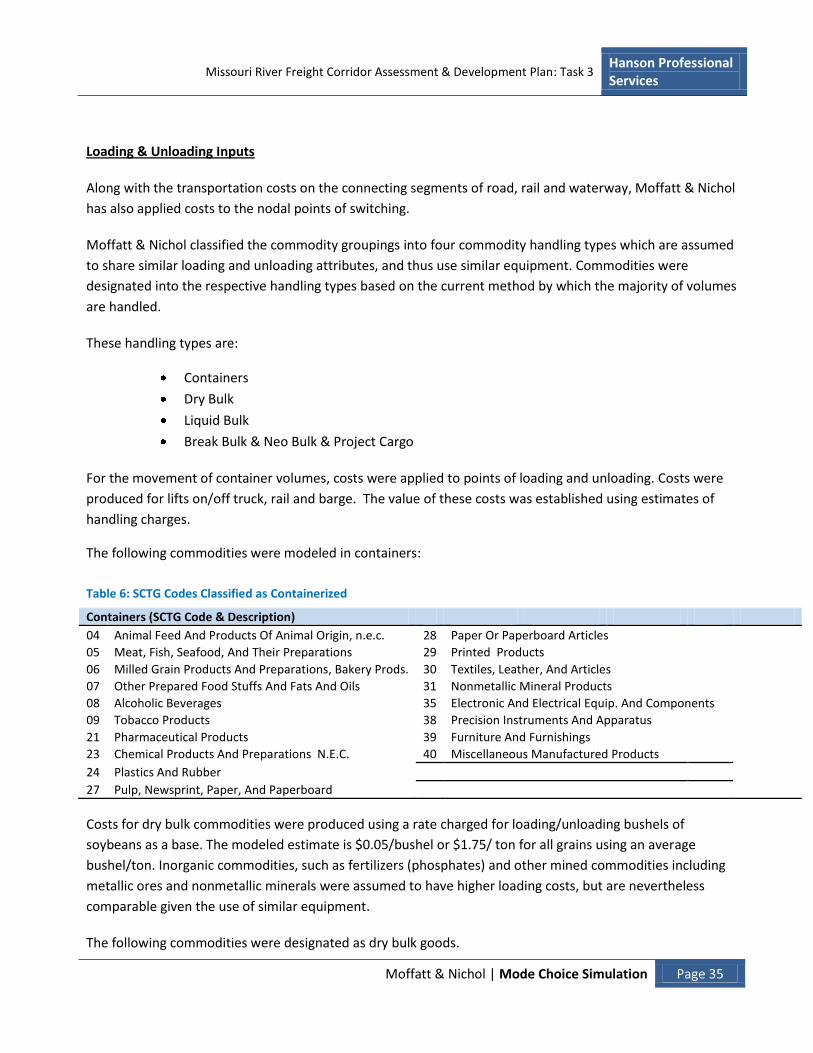
Loading & Unloading Inputs
Along with the transportation costs on the connecting segments of road, rail and waterway, Moffatt & Nichol
has also applied costs to the nodal points of switching.
Moffatt & Nichol classified the commodity groupings into four commodity handling types which are assumed
to share similar loading and unloading attributes, and thus use similar equipment. Commodities were
designated into the respective handling types based on the current method by which the majority of volumes
are handled.
These handling types are:
Containers
Dry Bulk
Liquid Bulk
Break Bulk & Neo Bulk & Project Cargo
For the movement of container volumes, costs were applied to points of loading and unloading. Costs were
produced for lifts on/off truck, rail and barge. The value of these costs was established using estimates of
handling charges.
The following commodities were modeled in containers:
Table 6: SCTG Codes Classified as Containerized
Containers (SCTG Code & Description)
04 Animal Feed And Products Of Animal Origin, n.e.c. 28 Paper Or Paperboard Articles
05 Meat, Fish, Seafood, And Their Preparations 29 Printed Products
06 Milled Grain Products And Preparations, Bakery Prods. 30 Textiles, Leather, And Articles
07 Other Prepared Food Stuffs And Fats And Oils 31 Nonmetallic Mineral Products
08 Alcoholic Beverages 35 Electronic And Electrical Equip. And Components
09 Tobacco Products 38 Precision Instruments And Apparatus
21 Pharmaceutical Products 39 Furniture And Furnishings
23 Chemical Products And Preparations N.E.C. 40 Miscellaneous Manufactured Products
24 Plastics And Rubber
27 Pulp, Newsprint, Paper, And Paperboard
Costs for dry bulk commodities were produced using a rate charged for loading/unloading bushels of
soybeans as a base. The modeled estimate is $0.05/bushel or $1.75/ ton for all grains using an average
bushel/ton. Inorganic commodities, such as fertilizers (phosphates) and other mined commodities including
metallic ores and nonmetallic minerals were assumed to have higher loading costs, but are nevertheless
comparable given the use of similar equipment.
The following commodities were designated as dry bulk goods.

Missouri River Freight Corridor Assessment & Development Plan: Task 3 Hanson Professional Services
Moffatt & Nichol | Mode Choice Simulation Page 36
Table 7: SCTG Codes Classified as Dry Bulk
Dry Bulk (SCTG Code & Description)
02 Cereal Grains 14 Metallic Ores And Concentrates
03 Other Agricultural Products 15 Coal
11 Natural Sands 20 Basic Chemicals
12 Gravel And Crushed Stone 22 Fertilizers
13 Nonmetallic Minerals n.e.c. 41 Waste And Scrap
Liquid bulk commodity costs were developed for truck, rail and barge, and represent the singular cost of the
“hook up” for respective transportation modes to the storage tank. Those commodities classified as liquid
bulk are:
Table 8: SCTG Codes Classified as Liquid Bulk
Liquid Bulk (SCTG Code & Description)
16 Crude Petroleum 18 Fuel Oils 17 Gasoline And Aviation Turbine Fuel 19 Coal And Petroleum Products, n.e.c.
Given the variation in the commodities classified as break bulk, neo bulk and project cargo, the costs of
loading/unloading has been modeled either on a per ton or per load basis. Forest Products, Wood Products,
Iron and Steel, were modeled by the load. For the remaining commodities a loading/unloading cost per ton is
applied.
Table 9: SCTG Codes Classified as Neo Bulk & Project Cargo
Break & Neo Bulk & Project Cargo (SCTG Code & Description)
10 Monumental Or Building Stone 33 Articles Of Base Metal
25 Logs And Other Wood In The Rough 34 Machinery
26 Wood Products 37 Transportation Equipment n.e.c.
32 Base Metal In Primary Forms And Basic Shapes

Missouri River Freight Corridor Assessment & Development Plan: Task 3 Hanson Professional Services
Moffatt & Nichol | Mode Choice Simulation Page 37
Inventory Carrying Cost
To measure the estimated inventory carrying cost, M&N used the inventory carrying cost percentages from
US Department of Transportation (USDOT) Federal Railroad Administration’s Intermodal Transportation and
Inventory Cost Model (ITIC-IM), as can be seen in Table 10. These percentages were multiplied by the value
of the shipment and by the days the shipment was in transit in order to get the inventory carrying cost for a
shipment.

Missouri River Freight Corridor Assessment & Development Plan: Task 3 Hanson Professional Services
Moffatt & Nichol | Mode Choice Simulation Page 38
Table 10: Inventory Carrying Cost by Commodity (STCC Code)
Two-digit Service Inventory Carrying Cost
STCC Description Percent Percentage
01 Farm products 95% 20%
08 Forest products 95% 20%
09 Fish 98% 20%
10 Metallic ores 90% 20%
11 Coal 90% 20%
13 Crude petroleum or natural gas 95% 30%
14 Non-metallic minerals 90% 20%
19 Ordnance or accessories 95% 35%
20 Food & kindred products 97% 30%
21 Tobacco products 95% 30%
22 Textile mill products 95% 20%
23 Apparel & other textile mill products 95% 30%
24 Lumber & wood products 90% 25%
25 Furniture & fixtures 95% 30%
26 Pulp, paper & allied products 90% 25%
27 Printing & publishing 95% 30%
28 Chemical & allied products 95% 25%
29 Petroleum & coal products 95% 20%
30 Rubber & misc. plastic products 95% 25%
31 Leather & leather products 95% 30%
32 Stone, clay & glass 90% 20%
33 Primary metal industries 90% 20%
34 Fabricated metal products 95% 30%
35 Industrial machinery & equipment 95% 30%
36 Electronic & other electrical equipment 95% 30%
37 Transportation equipment 95% 25%
38 Instruments & related products 95% 35%
39 Misc. mfg industries 95% 25%
40 Waste & scrap 90% 15%
41 Misc. freight shipments 95% 25%
42 Empty containers, shipping devices 90% 15%
43 Mail, express traffic 95% 30%
44 Freight forwarder traffic 95% 30%
45 Shipper assoc. or similar traffic 98% 30%
46 Misc. mixed shipments 95% 30%
47 Small package freight 95% 30%
48 Unknown Commodity 95% 30%
49 Hazardous materials 95% 25%
50 In bulk in boxcars 95% 25%
99 Mixed shipments 95% 25%
Source: US Department of Transportation; Federal Railroad Administration

Missouri River Freight Corridor Assessment & Development Plan: Task 3 Hanson Professional Services
Moffatt & Nichol | Application of Costs Page 39
8. Application of Costs
For trucking, a distinction is made between drayage (less than 100 miles) and long-haul (more than 100
miles). If a shipment goes by only truck, the trucking transportation costs are estimated on simply point-to-
point without inclusion of any handling charges. This also means that the inventory cost of trucking is based
only upon the time the truck is in transit.
The model also makes series of assumptions with respect to costs associated to rail. The rail cost is calculated
excluding loading/unloading and drayage costs. Most of the commodities moved by rail are bulk, and it is
assumed that the facilities acting as origins and destinations are located on a rail siding. This assumption
makes drays unnecessary and loading/unloading the responsibility of the shipper/receiver. This means that
the inventory cost for rail is based solely upon the time the rail is in transit.
Unlike what was assumed for rail and truck, the use of barge sometimes involves a third party facility and a
change in mode of transportation. Therefore, in some scenarios, drayage (to get the shipment to or from a
water port) and handling (to unload the trucks and load the barges or vice versa) were included in addition to
the cost of barge transportation. However, drayage and handling fees and wait times were not included for
an origin or destination if it was in a county that had a water port, or if the origin or destination was located
outside of the MRB. The dray/handling wasn’t included for an origin or destination if it was in a country with
a water port because, in these scenarios it was assumed that the facility would be on the water and therefore
wouldn’t need to truck the shipment to and from the water and could load the barge at their convenience.
The dray/handling wasn’t included for an origin or destination outside of the MRB because it was also
assumed that these facilities would be on the water, making a dray unnecessary and the loading or unloading
the responsibility of that party. In the situations where a dray and handling were incorporated, the total cost
of the barge trip would include the cost of the actual barge transportation, the trucking costs needed for
drayage, the handling costs, as well as the inventory cost involved for the time of the trip (which would
include the time of barging, the time of any trucking, and the wait times involved with any handling).
In addition, there were certain scenarios in which inventory cost was not included as part of the cost of the
shipment. Inventory cost was not included for Intra-regional shipments or for Outbound shipments that
were destined to be exports. This means that for these shipments, there was no inventory cost taken in to
account for rail, truck, or barge. The decision to remove the inventory costs from the exports was founded
on the assumption that in many cases the products are shipped FOB, and for most commodities that have
high barge potential, have high dwell times throughout the export process. Inventory costs were removed
from the Intra-regional movements because given the relatively short times and distances of the routes,
inventory carrying costs are not considered to be a significant constraint.

Missouri River Freight Corridor Assessment & Development Plan: Task 3 Hanson Professional Services
Moffatt & Nichol | Conclusions Page 40
9. Conclusions
Table 11 demonstrates how the additional costs and wait times associated with barging in the model can
impact the affordability of transporting goods via barge verses other modes. This table analyzes the 3,382
barge eligible O&D pairings (which is the data before elimination criteria D was enforced). The left half of the
table provides the transportation costs (defined here as all costs except inventory cost) and the inventory
costs associated with the different modes of transportation considering only the costs incurred during the
time spent on that mode (on only rail, barge, or truck). These costs are expressed as a percentage of
shipment value. The right half of the table demonstrates the impact of adding drayage and handling costs to
the barge transportation cost as well as adding in the time of draying and the wait times involved with
switching modes for barge to the inventory costs for barge (Note: the drayage and handling costs and wait
times were added to all barge movements, even if some of these fees and times were later excluded from
certain shipments for analysis purposes).
Table 11: Cost Comparison Between Modes
Excludes Dray and Handling Includes Dray and Handling
Transport Costs as a percent of Shipment
Value
Inventory Carrying Costs as a percent of
Shipment Value
Transport Costs as a percent of Shipment
Value
Inventory Carrying Costs as a percent of
Shipment Value
Barge 3.8% 133.3% 9.5% 215.6%
Rail 4.7% 13.7% 4.7% 13.7%
Truck 13.5% 18.6% 13.5% 18.6% Source: Moffatt & Nichol
The left hand side of the table shows that when the shipments don’t include dray/handling, barge
transportation costs equate to 3.8% of the value of the shipment. This makes barge the cheapest form of
transportation for shipments.
However, when including dray/handling, the total transportation costs of the intermodal barge movement
jumps to 9.5% of the value of the shipment. At this level barge is no longer the cheapest mode of
transportation. Thus the added cost of the dray/handling makes the barge alternative not as attractive for
shipments.
Barge becomes the most expensive form of transportation when the inventory carrying costs are applied. As
a result this limits the types of goods which can potentially be barged to low value commodities, which can
dwell for extensive periods without incurring high inventory costs.
Given the information presented in Table 11 showing the impact of inventory costs on barge shipments, it is
not surprising that Outbound shipments represent the majority of potential volumes (

Missouri River Freight Corridor Assessment & Development Plan: Task 3 Hanson Professional Services
Moffatt & Nichol | Conclusions Page 41
Figure 24) in that, as explained above in the screening criteria, inventory costs were removed from exports as
well as Intra-regional shipments.
Total Potential
Moffatt & Nichol estimates that approximately 59 million total tonnes of annual commodity shipments could
potentially move by barge on the Missouri River as noted in
Figure 24. By shipment type, 75% of this potential is accounted for by Outbound shipments. Intra-regional
shipments represent nearly all of the remaining tonnage. In part, the dominance of these two shipment types
can be explained by the model criteria which excluded inventory costs associated with foreign bound exports
and Intra-regional movements.
Inventory carrying costs can be a burdensome expense when barging, particularly if there are additional
drays and wait times involved. It is therefore not surprising that so many of the potential Missouri River
barge shipments do not meet the criteria for inventory carrying cost.
Figure 24: Potential Missouri River Barge Volume by Shipment Type
Source: Moffatt & Nichol
By commodity, it can be seen that cereal grains and other agricultural products account for roughly 75% of
the total potential. It is not surprising that these two commodity groups represent such a large share given
that there is a substantial volume of production in counties adjacent to the River. Furthermore, shipments
are typically in large tonnages, an attribute which favors barge. The identified shipments of these two
commodity groups are either exports or intra-regional movements, meaning that they did not have an
Outbound75%
Intra-regional
24%
Inbound1%
Total Tonnage = 59 million tonnes

Missouri River Freight Corridor Assessment & Development Plan: Task 3 Hanson Professional Services
Moffatt & Nichol | Conclusions Page 42
inventory carrying cost levied against them, which helped make the overall price of moving the shipment
lower.
Figure 25: Potential Missouri River Barge Volume by Commodity
Source: Moffatt & Nichol
Figure 26 illustrates the commodity flows of the potential shipments for all three shipment types and all identified commodities. The map shows the counties/FAF regions of origin and counties/FAF regions of destination. Several notable observations can be made:
Within MRB, the majority of origin and destination counties are located adjacent to the Missouri
River.
Outbound shipments are destined to southern port regions, (denoted in blue) including New Orleans
and Mobile Alabama, and are likely foreign exports. These shipments represent the heaviest flow.
Inbound shipments originate from three regions in Alabama, Tennessee and Illinois respectively.
These are primarily shipments of coal and gravel.
Other ag prods.46%Cereal grains
29%
Coal-n.e.c. & Petro goods
n.ec.11%
Nonmetal mineral
products3%
Other11%
Total Tonnage = 59 million tonnes

Missouri River Freight Corridor Assessment & Development Plan: Task 3 Hanson Professional Services
Moffatt & Nichol | Conclusions Page 43
Figure 26: Potential Commodity Flow Routes
Source: Moffatt & Nichol
The commodity and routes of the three shipment types are addressed and discussed in greater detail in
Figure 27 through Figure 32.
Outbound Potential
Given that Outbound shipments made up the majority of the potential Missouri River barge volumes, it
should not be surprising that the commodity composition of the Outbound shipments is similar to the overall
commodity make-up. Other agricultural products, cereal grains, and coal and petroleum products n.e.c.
account for almost all of the tonnage. The routes of these shipments can be seen in Figure 28, and again it

Missouri River Freight Corridor Assessment & Development Plan: Task 3 Hanson Professional Services
Moffatt & Nichol | Conclusions Page 44
becomes evident that the majority of these head south for eventual exportation. The counties from which
these shipments originate tend to be on or close to the Missouri River, further enforcing the importance of
no or little dray in order to keep a barge movement competitive.
Figure 27: Commodity Composition of Potential Outbound Shipments
Source: Moffatt & Nichol
Other ag prods.56%
Cereal grains29%
Coal-n.e.c.& Petro
Goods-n.e.c..15%
Machinery0%
InterO Tonnage = 44 Million

Missouri River Freight Corridor Assessment & Development Plan: Task 3 Hanson Professional Services
Moffatt & Nichol | Conclusions Page 45
Figure 28: Potential Outbound Commodity Flow Routes
Source: Moffatt & Nichol
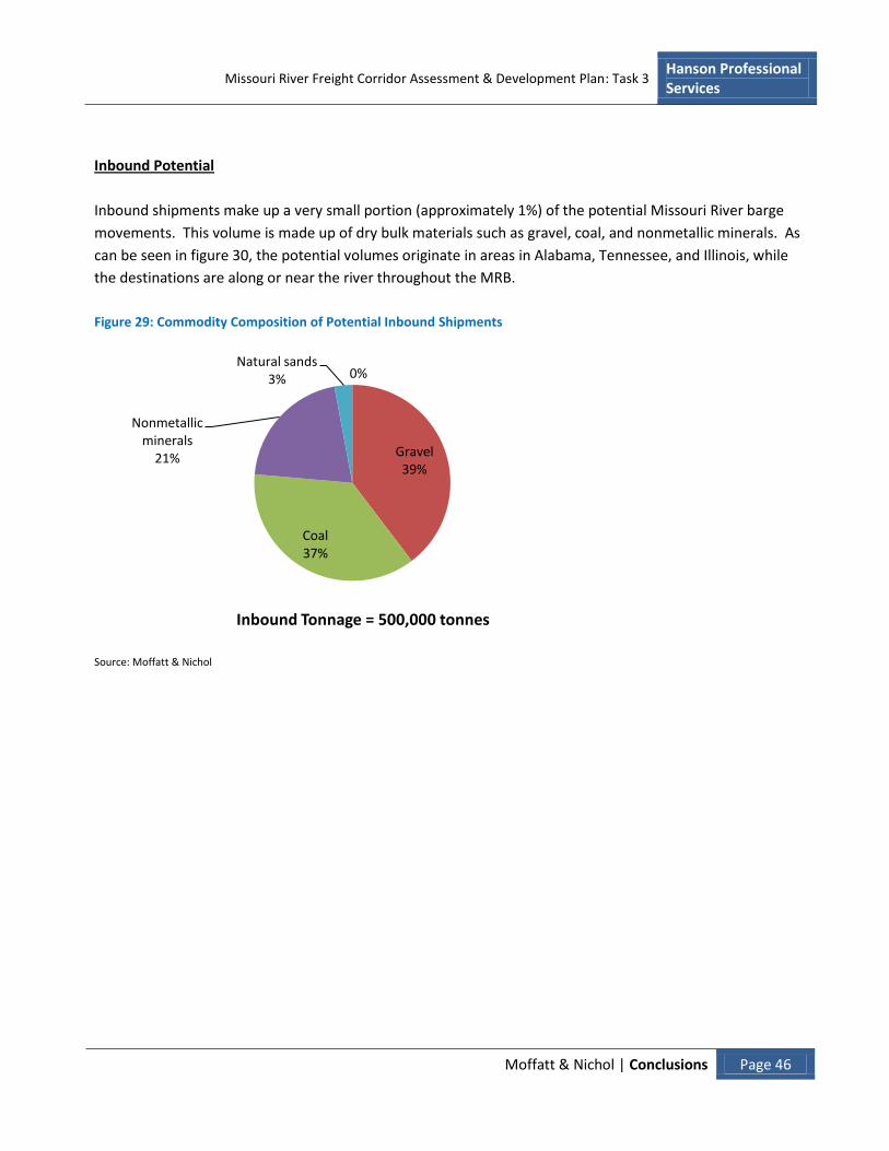
Missouri River Freight Corridor Assessment & Development Plan: Task 3 Hanson Professional Services
Moffatt & Nichol | Conclusions Page 46
Inbound Potential
Inbound shipments make up a very small portion (approximately 1%) of the potential Missouri River barge
movements. This volume is made up of dry bulk materials such as gravel, coal, and nonmetallic minerals. As
can be seen in figure 30, the potential volumes originate in areas in Alabama, Tennessee, and Illinois, while
the destinations are along or near the river throughout the MRB.
Figure 29: Commodity Composition of Potential Inbound Shipments
Source: Moffatt & Nichol
0%
Gravel39%
Coal37%
Nonmetallic minerals
21%
Natural sands3%
Inbound Tonnage = 500,000 tonnes

Missouri River Freight Corridor Assessment & Development Plan: Task 3 Hanson Professional Services
Moffatt & Nichol | Conclusions Page 47
Figure 30: Potential Inbound Commodity Flow Routes
Source: Moffatt & Nichol
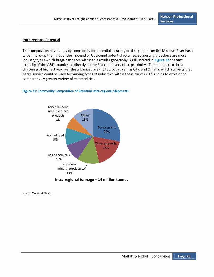
Missouri River Freight Corridor Assessment & Development Plan: Task 3 Hanson Professional Services
Moffatt & Nichol | Conclusions Page 48
Intra-regional Potential
The composition of volumes by commodity for potential Intra-regional shipments on the Missouri River has a wider make-up than that of the Inbound or Outbound potential volumes, suggesting that there are more industry types which barge can serve within this smaller geography. As illustrated in Figure 32 the vast majority of the O&D counties lie directly on the River or in very close proximity. There appears to be a clustering of high activity near the urbanized areas of St. Louis, Kansas City, and Omaha, which suggests that barge service could be used for varying types of industries within these clusters. This helps to explain the comparatively greater variety of commodities.
Figure 31: Commodity Composition of Potential Intra-regional Shipments
Source: Moffatt & Nichol
Cereal grains28%
Other ag prods.18%
Nonmetal mineral products
13%
Basic chemicals10%
Animal feed10%
Miscellaneous manufactured
products8%
Other13%
Intra-regional tonnage = 14 million tonnes
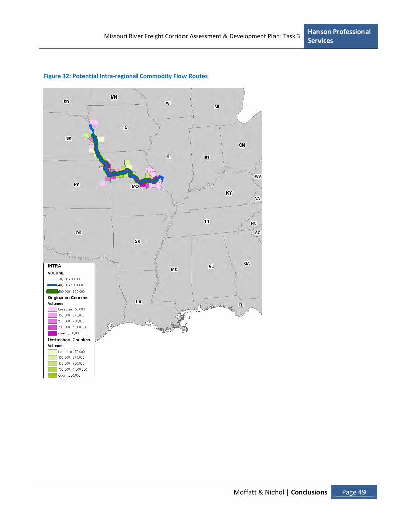
Missouri River Freight Corridor Assessment & Development Plan: Task 3 Hanson Professional Services
Moffatt & Nichol | Conclusions Page 49
Figure 32: Potential Intra-regional Commodity Flow Routes
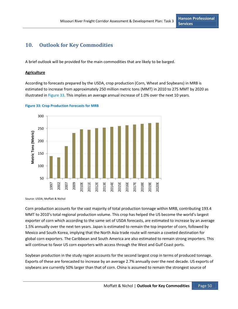
Missouri River Freight Corridor Assessment & Development Plan: Task 3 Hanson Professional Services
Moffatt & Nichol | Outlook for Key Commodities Page 50
10. Outlook for Key Commodities
A brief outlook will be provided for the main commodities that are likely to be barged.
Agriculture
According to forecasts prepared by the USDA, crop production (Corn, Wheat and Soybeans) in MRB is
estimated to increase from approximately 250 million metric tons (MMT) in 2010 to 275 MMT by 2020 as
illustrated in Figure 33. This implies an average annual increase of 1.0% over the next 10 years.
Figure 33: Crop Production Forecasts for MRB
Source: USDA; Moffatt & Nichol
Corn production accounts for the vast majority of total production tonnage within MRB, contributing 193.4
MMT to 2010’s total regional production volume. This crop has helped the US become the world’s largest
exporter of corn which according to the same set of USDA forecasts, are estimated to increase by an average
1.5% annually over the next ten years. Japan is estimated to remain the top importer of corn, followed by
Mexico and South Korea, implying that the North Asia trade route will remain a coveted destination for
global corn exporters. The Caribbean and South America are also estimated to remain strong importers. This
will continue to favor US corn exporters with access through the West and Gulf Coast ports.
Soybean production in the study region accounts for the second largest crop in terms of produced tonnage.
Exports of these are forecasted to increase by an average 2.7% annually over the next decade. US exports of
soybeans are currently 50% larger than that of corn. China is assumed to remain the strongest source of
50
100
150
200
250
300
19
97
20
02
20
07
20
09
20
10
E
20
11
E
20
12
E
20
13
E
20
14
E
20
15
E
20
16
E
20
17
E
20
18
E
20
19
E
20
20
E
Me
tric
To
ns
(Me
tric
)
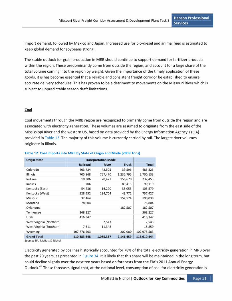
Missouri River Freight Corridor Assessment & Development Plan: Task 3 Hanson Professional Services
Moffatt & Nichol | Outlook for Key Commodities Page 51
import demand, followed by Mexico and Japan. Increased use for bio-diesel and animal feed is estimated to
keep global demand for soybeans strong.
The stable outlook for grain production in MRB should continue to support demand for fertilizer products
within the region. These predominantly come from outside the region, and account for a large share of the
total volume coming into the region by weight. Given the importance of the timely application of these
goods, it is has become essential that a reliable and consistent freight corridor be established to ensure
accurate delivery schedules. This has proven to be a detriment to movements on the Missouri River which is
subject to unpredictable season draft limitations.
Coal
Coal movements through the MRB region are recognized to primarily come from outside the region and are
associated with electricity generation. These volumes are assumed to originate from the east side of the
Mississippi River and the western US, based on data provided by the Energy Information Agency’s (EIA)
provided in Table 12. The majority of this volume is currently carried by rail. The largest river volumes
originate in Illinois.
Table 12: Coal Imports into MRB by State of Origin and Mode (2008 Tons)
Origin State Transportation Mode
Railroad River Truck Total
Colorado 403,724 42,505 39,596 485,825
Illinois 705,868 757,470 1,236,795 2,700,133
Indiana 10,306 70,477 156,670 237,453
Kansas 706 89,413 90,119
Kentucky (East) 54,236 16,290 33,053 103,579
Kentucky (West) 528,952 184,704 43,771 757,427
Missouri 32,464 157,574 190,038
Montana 78,804 78,804
Oklahoma 182,507 182,507
Tennessee 368,227 368,227
Utah 416,347 416,347
West Virginia (Northern) 2,543 2,543
West Virginia (Southern) 7,511 11,348 18,859
Wyoming 107,776,503 202,080 107,978,583
Grand Total 110,383,648 1,085,337 2,141,459 113,610,444 Source: EIA; Moffatt & Nichol
Electricity generated by coal has historically accounted for 78% of the total electricity generation in MRB over
the past 20 years, as presented in Figure 34. It is likely that this share will be maintained in the long term, but
could decline slightly over the next ten years based on forecasts from the EIA’s 2011 Annual Energy
Outlook.viii These forecasts signal that, at the national level, consumption of coal for electricity generation is

Missouri River Freight Corridor Assessment & Development Plan: Task 3 Hanson Professional Services
Moffatt & Nichol | Outlook for Key Commodities Page 52
estimated to remain essentially flat between 2010 and 2020, however long-term forecasts which extend to
2035, call for coal consumption to maintain its current share of total energy consumption of 21% as
illustrated in Figure 35.
Figure 34: Electricity Generation in MRB (Million Megawatt Hours)
Source: EIA; Moffatt & Nichol
Figure 35: Primary Energy Consumption Forecasts
Source: EIA
0
50
100
150
200
250
19
90
19
92
19
94
19
96
19
98
20
00
20
02
20
04
20
06
20
08
MM
Wh
Total
Coal
0
20
40
60
80
100
120
19
90
19
95
20
00
20
05
20
10
20
15
E
20
20
E
20
25
E
20
30
E
20
35
E
Qu
adri
llio
n B
tu p
er
year
Renewables
Coal
Natural Gas
Biofuels
Liquids
Nuclear
Missouri River Freight Corridor Assessment & Development Plan: Task 3 Hanson Professional Services
Moffatt & Nichol | Outlook for Key Commodities Page 53
Aggregate, Sand and Gravel
The use of aggregate, sand and gravel in MRB are predominantly associated with regional construction
activity. While it is assumed that some volume is used in the construction in the residential sector the
majority of use occurs on sites of large non-residential and heavy construction projects. These include
private, state and federally funded projects.
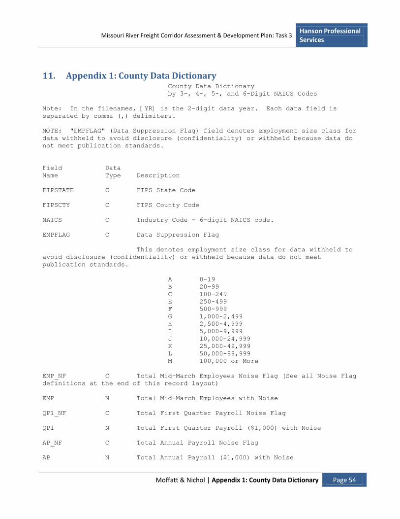
Missouri River Freight Corridor Assessment & Development Plan: Task 3 Hanson Professional Services
Moffatt & Nichol | Appendix 1: County Data Dictionary Page 54
11. Appendix 1: County Data Dictionary County Data Dictionary
by 3-, 4-, 5-, and 6-Digit NAICS Codes
Note: In the filenames, [YR] is the 2-digit data year. Each data field is
separated by comma (,) delimiters.
NOTE: "EMPFLAG" (Data Suppression Flag) field denotes employment size class for
data withheld to avoid disclosure (confidentiality) or withheld because data do
not meet publication standards.
Field Data
Name Type Description
FIPSTATE C FIPS State Code
FIPSCTY C FIPS County Code
NAICS C Industry Code - 6-digit NAICS code.
EMPFLAG C Data Suppression Flag
This denotes employment size class for data withheld to
avoid disclosure (confidentiality) or withheld because data do not meet
publication standards.
A 0-19
B 20-99
C 100-249
E 250-499
F 500-999
G 1,000-2,499
H 2,500-4,999
I 5,000-9,999
J 10,000-24,999
K 25,000-49,999
L 50,000-99,999
M 100,000 or More
EMP_NF C Total Mid-March Employees Noise Flag (See all Noise Flag
definitions at the end of this record layout)
EMP N Total Mid-March Employees with Noise
QP1_NF C Total First Quarter Payroll Noise Flag
QP1 N Total First Quarter Payroll ($1,000) with Noise
AP_NF C Total Annual Payroll Noise Flag
AP N Total Annual Payroll ($1,000) with Noise

Missouri River Freight Corridor Assessment & Development Plan: Task 3 Hanson Professional Services
Moffatt & Nichol | Appendix 1: County Data Dictionary Page 55
EST N Total Number of Establishments
N1_4 N Number of Establishments: 1-4 Employee Size Class
N5_9 N Number of Establishments: 5-9 Employee Size Class
N10_19 N Number of Establishments: 10-19 Employee Size Class
N20_49 N Number of Establishments: 20-49 Employee Size Class
N50_99 N Number of Establishments: 50-99 Employee Size Class
N100_249 N Number of Establishments: 100-249 Employee Size Class
N250_499 N Number of Establishments: 250-499 Employee Size Class
N500_999 N Number of Establishments: 500-999 Employee Size Class
N1000 N Number of Establishments: 1,000 or More Employee Size
Class
N1000_1 N Number of Establishments: Employment Size Class:
1,000-1,499 Employees
N1000_2 N Number of Establishments: Employment Size Class:
1,500-2,499 Employees
N1000_3 N Number of Establishments: Employment Size Class:
2,500-4,999 Employees
N1000_4 N Number of Establishments: Employment Size Class:
5,000 or More Employees
CENSTATE C Census State Code
CENCTY C Census County Code
NOTE: Noise Flag definitions (fields ending in _NF) are:
G 0 to < 2% noise (low noise)
H 2 to < 5% noise (medium noise)
D Withheld to avoid disclosing data for individual companies; data
are included in higher level totals. Employment or payroll field set to zero.
S Withheld because estimate did not meet publication standards.
Employment or payroll field set to zero.

Missouri River Freight Corridor Assessment & Development Plan: Task 3 Hanson Professional Services
Moffatt & Nichol | Appendix 2: Economic Overview Appendix Page 56
12. Appendix 2: Economic Overview Appendix
12.1. Geographic & Trade Volumes
As noted in the Executive Summary, Moffatt & Nichol considers the region of interest to be the territory
encompassed by:
Missouri
Iowa
South Dakota
Nebraska
Kansas
These states border the navigable portion of the Missouri River, and are most pertinent to assessing
potential commercial activity.
Figure 36: MRB Region (Selected States Denoted in Dark Green)
St. LouisKansas City
Omaha
Wichita
Lincoln
JoplinSpringfield
Topeka
Des Moines
Columbia
Davenport
Sioux City
Sioux Falls
Iowa City
Waterloo
St. Joseph
Dubuque
Rapid City
Cedar RapidsAmes
Jefferson City

Missouri River Freight Corridor Assessment & Development Plan: Task 3 Hanson Professional Services
Moffatt & Nichol | Appendix 2: Economic Overview Appendix Page 57
Moffatt & Nichol has used data from FAF, to determine the level of trade which occurs with MRB. As
discussed, the FAF data provides volume of trade by commodity, mode, and direction (import & export,
domestic & foreign) between geographic regions.
Trade volume which originates in and is destined to MRB, by direction is presented Table 13 and Table 14.
The majority of trade volume which originates in MRB is destined to locations within the region, as noted in
Table 13. These represent Intra-regional moves, or comparatively short distance routes, and therefore it is
not surprising that 95% of this trade is carried on trucks. While there are some of these Intra-regional
volumes being barged, given the speed and versatility advantage of trucking within a small geography, it is
unlikely that much of this Intra-regional volume will be switched over to barge.
For the remaining Inter0 trade volume, which is destined to locations outside MRB, the greatest share is
headed to the South of which approximately 25% of the total is carried by barge. Nevertheless, the combined
volume carried by rail and truck still accounts for the majority of trade destined to the South, roughly 65%,
and therefore it would be assumed that in this combined tonnage there are likely some shipments which
could benefit from switching to barge. The South is also the most import gateway region for international
exports originating within the MRB, accounting for almost half of the total, and therefore barge movements
could be incorporated into international supply chains.
Table 13: Shipments Originating in MRB (Tons 1,000s)
Mode East MRB North Northeast Northwest South Southeast Southwest West Total
Truck 47,705 1,012,440 54,010 8,113 6,985 40,481 6,482 2,121 11,439 1,189,777
Rail 6,275 20,241 7,632 5,678 5,122 43,693 2,561 1,840 12,844 105,887
Water* 8,882 4,114 0 8 41 30,261 3,213 5 2 46,527
Air (include truck-air) 14 14 4 16 6 11 13 0 24 102
Multiple modes & mail 4,827 6,112 1,530 1,233 899 7,924 1,189 381 4,596 28,690
Pipeline 1,899 4,687 1,012 1,268 1,092 5,139 810 383 1,956 18,246
Other and unknown 496 14,155 352 301 135 1,371 98 65 829 17,801
Total 70,098 1,061,762 64,540 16,616 14,281 128,881 14,366 4,795 31,690 1,407,030
Type
East MRB North Northeast Northwest South Southeast Southwest West Total
Domestic Only
69,478 1,061,734 53,173 15,425 10,753 107,972 13,800 4,648 28,988 1,365,970
Import
1 20 0 0 0 0 0 0 0 21
Export
619 9 11,367 1,191 3,527 20,909 566 148 2,702 41,039
Total
70,098 1,061,762 64,540 16,616 14,281 128,881 14,366 4,795 31,690 1,407,030
* Includes Iowa and St. Louis volumes carried on the Mississippi River MRB as a column header indicates within MRB flows Source: FAF; Moffatt & Nichol

Missouri River Freight Corridor Assessment & Development Plan: Task 3 Hanson Professional Services
Moffatt & Nichol | Appendix 2: Economic Overview Appendix Page 58
As identified in Table 13, the majority of MRB’s total trade volumes are Intra-regional moves, originating and destined to locations within MRB. Therefore, in the MRB column of Table 14 the same volume of trade by mode and type is shown as in Table 13.
For the remaining Inbound trade, which originates outside the MRB, the majority of this volume is carried by
rail from the Northwest. This region is not readily accessible via inland waterways. The East and South also
account for a large share of Inbound trade, of which most of the respective volumes are carried by truck;
though not surprisingly there is a significant volume of pipeline commodities, presumably petro goods,
originating in the South as well. While these petro goods could potentially be carried via barge, these would
have to compete with existing low cost pipeline services.
Table 14: Shipments Destined to MRB (Tons 1,000s)
Mode East MRB North Northeast Northwest South Southeast Southwest West Total
Truck 45,406 1,012,440 37,911 4,996 5,107 29,600 4,700 1,314 8,055 1,149,528
Rail 6,242 20,241 8,796 181 103,256 10,019 1,396 186 4,435 154,753
Water* 1,711 4,114 0 0 496 845 0 0 0 7,167
Air (include truck-air) 8 14 2 8 1 3 1 1 6 43
Multiple modes & mail 6,064 6,112 1,128 520 29,061 1,470 336 66 1,832 46,587
Pipeline 6,122 4,687 1,164 1,998 5,031 15,689 579 1,900 2,733 39,904
Other and unknown 203 14,155 290 71 25 223 29 17 214 15,226
Total 65,757 1,061,762 49,290 7,774 142,978 57,848 7,041 3,483 17,276 1,413,209
Type East MRB North Northeast Northwest South Southeast Southwest West Total
Domestic Only
64,972 1,061,734 42,867 6,594 141,718 55,422 6,422 3,470 15,207 1,398,406
Import
784 20 6,423 1,180 1,260 2,427 619 13 2,069 14,794
Export
0 9 0 0 0 0 0 0 0 9
Total
65,757 1,061,762 49,290 7,774 142,978 57,848 7,041 3,483 17,276 1,413,209
* Includes Iowa and St. Louis volumes carried on the Mississippi River
Source: FAF; Moffatt & Nichol

Missouri River Freight Corridor Assessment & Development Plan: Task 3 Hanson Professional Services
Moffatt & Nichol | 11BAppendix 2: Economic Overview Appendix Page 59
12.2. Economics
MRB’s Real Gross Domestic Product (GDP, excludes inflation) has accounted for an average 4.4% of the national total over the past three years for which data is available. This share is down slightly from an average 4.6% during the late 1990’s, suggesting that economic growth within the study region has slightly lagged that of the rest of the country over the past decade. This is due in part to the region’s relatively lower exposure to the sectors which led periods of high national growth, namely the technology boom in the late 1990’s and housing in the latter half of the 2000’s. This relative exposure has, however, helped the region remain comparatively more stable during this same period as identified Figure 37, and has allowed it to fare comparatively better in the most recent downturn.
Figure 37: Annual real GDP growth for the US and MRB
Source: Bureau of Economic Analysis; Moffatt & Nichol
MRB’s economy has a greater exposure to the Agriculture and Manufacturing broad sectors by comparison to the US as a whole, as illustrated in Figure 38.
-3%
-2%
-1%
0%
1%
2%
3%
4%
5%
6%
1998
1999
2000
2001
2002
2003
2004
2005
2006
2007
2008
2009
2010
E
US
MRB

Missouri River Freight Corridor Assessment & Development Plan: Task 3 Hanson Professional Services
Moffatt & Nichol | 11BAppendix 2: Economic Overview Appendix Page 60
This Page Intentionally Left Blank

Missouri River Freight Corridor Assessment & Development Plan: Task 3 Hanson Professional Services
Moffatt & Nichol | Appendix 2: Economic Overview Appendix Page 61
Figure 38: Composition of GDP by Broad Sectors (2009)
Source: Bureau of Economic Analysis; Moffatt & Nichol
As discussed earlier in the report, trade volumes to and from MRB will be driven by the production output of
the region’s industries, as well as by demand for and consumption of intermediate production inputs and
final goods. The commodity being shipped will be determined by the industry by which it is being either
produced or demanded. Therefore, Table 15 through Table 17 present the top goods producing industries
and intermediate inputs within the MRB region. These lists are provided in the context of regional production
and consumption/attraction.
Production
Table 15 provides a list of the top 20 goods producing industries in the study area by value in 2007, as
Moffatt & Nichol estimates using data from the CBP. The industry mix is quite broad encompassing high-
value electronics manufacturing to high-value food products. There are several liquid bulk industries as well,
which could lend themselves to potential barge, assuming seasonal shipments are permitted. Agriculture is
not listed as it is not part of the CBP data set.
Not surprisingly the industries with the greatest production values include high value commodities such as
autos, aircraft and construction machinery manufacturing. Other large industries include chemicals,
pesticides, plastics and animal products.
0%
2%
4%
6%
8%
10%
12%
14%
16%
Agr
icu
ltu
re, F
FH*
Min
ing
Uti
litie
s
Co
nst
ruct
ion
Man
ufa
ctu
rin
g
US
MRB

Missouri River Freight Corridor Assessment & Development Plan: Task 3 Hanson Professional Services
Moffatt & Nichol | Appendix 2: Economic Overview Appendix Page 62
Table 15: Top 20 Goods Producing Industries by Value of Shipments: 2007, millions of dollars
Rank NAICS NAICS Definition Value
1 336112 Light Truck and Utility Vehicle Manufacturing 24,173.65
2 311611 Animal (except Poultry) Slaughtering 18,940.87
3 336411 Aircraft Manufacturing 12,350.66
4 333120 Construction Machinery Manufacturing 10,321.16
5 325193 Ethyl Alcohol Manufacturing 9,421.69
6 324110 Petroleum Refineries 9,168.86
7 333111 Farm Machinery and Equipment Manufacturing 8,688.34
8 325412 Pharmaceutical Preparation Manufacturing 6,900.72
9 336111 Automobile Manufacturing 5,353.83
10 334511 Search, detection, navigation, guidance…instrument manufacturing 4,910.52
11 511110 Newspaper Publishers 4,826.03
12 325611 Soap and Other Detergent Manufacturing 4,734.11
13 326199 All Other Plastics Product Manufacturing 4,723.67
14 333415 Air-Conditioning and Warm Air Heating Equipment...Manufacturing 4,275.94
15 511120 Periodical Publishers 4,197.58
16 325199 All Other Basic Organic Chemical Manufacturing 3,687.92
17 211111 Crude Petroleum and Natural Gas Extraction 3,053.38
18 311612 Meat Processed from Carcasses 3,016.16
19 325320 Pesticide and Other Agricultural Chemical Manufacturing 3,002.45
20 331315 Aluminum sheet, plate, and foil manufacturing 2,959.38 Source: Moffatt & Nichol based on 2007 Economic Census and 2007 County Business Patterns
Table 16 shows the top 20 goods producing industries by number of establishments within the study area.
The list looks very different from Table 15 above in that it is composed of a very broad mix of goods with a
much lower average production value. It also includes more heavy-bulk/low-value of goods industries in
mining, forest products, quarried products including crushed stone, and natural sands.
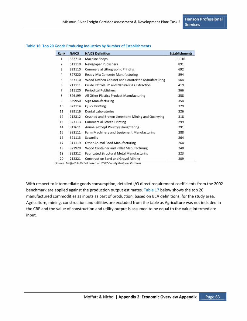
Missouri River Freight Corridor Assessment & Development Plan: Task 3 Hanson Professional Services
Moffatt & Nichol | Appendix 2: Economic Overview Appendix Page 63
Table 16: Top 20 Goods Producing Industries by Number of Establishments
Rank NAICS NAICS Definition Establishments
1 332710 Machine Shops 1,016
2 511110 Newspaper Publishers 891
3 323110 Commercial Lithographic Printing 692
4 327320 Ready-Mix Concrete Manufacturing 594
5 337110 Wood Kitchen Cabinet and Countertop Manufacturing 564
6 211111 Crude Petroleum and Natural Gas Extraction 419
7 511120 Periodical Publishers 366
8 326199 All Other Plastics Product Manufacturing 358
9 339950 Sign Manufacturing 354
10 323114 Quick Printing 329
11 339116 Dental Laboratories 326
12 212312 Crushed and Broken Limestone Mining and Quarrying 318
13 323113 Commercial Screen Printing 299
14 311611 Animal (except Poultry) Slaughtering 291
15 333111 Farm Machinery and Equipment Manufacturing 288
16 321113 Sawmills 264
17 311119 Other Animal Food Manufacturing 264
18 321920 Wood Container and Pallet Manufacturing 240
19 332312 Fabricated Structural Metal Manufacturing 223
20 212321 Construction Sand and Gravel Mining 209 Source: Moffatt & Nichol based on 2007 County Business Patterns
With respect to intermediate goods consumption, detailed I/O direct requirement coefficients from the 2002
benchmark are applied against the production output estimates. Table 17 below shows the top 20
manufactured commodities as inputs as part of production, based on BEA definitions, for the study area.
Agriculture, mining, construction and utilities are excluded from the table as Agriculture was not included in
the CBP and the value of construction and utility output is assumed to be equal to the value intermediate
input.

Missouri River Freight Corridor Assessment & Development Plan: Task 3 Hanson Professional Services
Moffatt & Nichol | Appendix 2: Economic Overview Appendix Page 64
Table 17: Top 20 Manufactured Commodity Inputs by Value
Rank Commodity Commodity Description Value
1 336300 Motor vehicle parts manufacturing 16,473
2 331110 Iron and steel mills and ferroalloy manufacturing 5,422
3 31161A Animal … slaughtering, rendering, and processing 4,322
4 325190 Other basic organic chemical manufacturing 4,138
5 324110 Petroleum refineries 2,659
6 32619A Other plastics product manufacturing 2,549
7 325211 Plastics material and resin manufacturing 2,386
8 322120 Paper mills 2,345
9 325110 Petrochemical manufacturing 2,317
10 334413 Semiconductor and … manufacturing 2,275
11 322210 Paperboard container manufacturing 2,068
12 336412 Aircraft engine and engine parts manufacturing 1,943
13 336413 Other aircraft parts … equipment manufacturing 1,879
14 333618 Other engine equipment manufacturing 1,805
15 326110 Plastics packaging materials … manufacturing 1,495
16 33131A Alumina refining and primary aluminum production 1,414
17 33291A Valve and fittings other than plumbing 1,375
18 334418 Printed circuit assembly ... manufacturing 1,324
19 332710 Machine shops 1,321
20 33131B Aluminum product manufacturing … 1,231 Source: Moffatt & Nichol
Consumption
Moffatt & Nichol evaluates goods attraction based primarily on consumer goods and goods required for
intermediate production. Goods consumption by households is based on retail sales which are realized in the
form of final goods sold. As discussed in the model process, these goods can be handled by smaller retail
establishments or indirectly via wholesalers.
Figure 39 provides concentrations in the wholesale industry within MRB. As expected, the highest
concentrations of firms are located in direct proximity to urban areas. The study area does have a large
number of wholesale firms located throughout it. This is due to the area’s high level of production of
agricultural goods, which are largely traded through wholesale firms.

Hanson Professional Services
Missouri River Freight Corridor Assessment & Development Plan: Task 3
Moffatt & Nichol | Appendix 2: Economic Overview Appendix Page 65
1998
1999
2000
2001
2002
2003
2004
2005
2006
2007
2008
2009
20
10E
Figure 39: County Distribution Wholesale Establishments
Source: Moffatt & Nichol based on 2007 Economic Census and 2007 County Business Patterns
As illustrated in Figure 40, regional income growth tends to trend with the national pattern. Since 1998 income in MRB has grown at a 4.4% CAGR as compared to the 4.7% CAGR experienced nationally. Therefore it would be expected that future retail sales within the regional should trend with or slightly below the national average.
Figure 40: Growth of Personal Income for US and MRB
10%
8%
6%
4%
2% US
MRB 0%
-2%
-4%
Source: Bureau of Economic Analysis
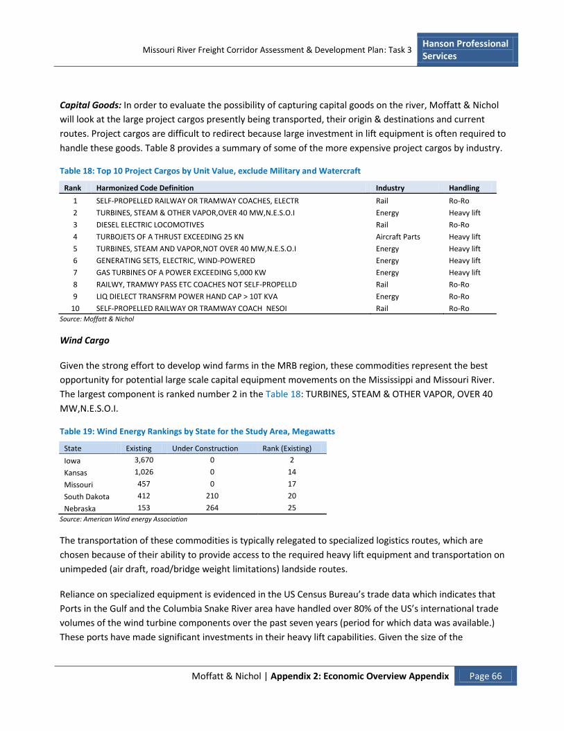
Missouri River Freight Corridor Assessment & Development Plan: Task 3 Hanson Professional Services
Moffatt & Nichol | Appendix 2: Economic Overview Appendix Page 66
Capital Goods: In order to evaluate the possibility of capturing capital goods on the river, Moffatt & Nichol
will look at the large project cargos presently being transported, their origin & destinations and current
routes. Project cargos are difficult to redirect because large investment in lift equipment is often required to
handle these goods. Table 8 provides a summary of some of the more expensive project cargos by industry.
Table 18: Top 10 Project Cargos by Unit Value, exclude Military and Watercraft
Rank Harmonized Code Definition Industry Handling
1 SELF-PROPELLED RAILWAY OR TRAMWAY COACHES, ELECTR Rail Ro-Ro
2 TURBINES, STEAM & OTHER VAPOR,OVER 40 MW,N.E.S.O.I Energy Heavy lift
3 DIESEL ELECTRIC LOCOMOTIVES Rail Ro-Ro
4 TURBOJETS OF A THRUST EXCEEDING 25 KN Aircraft Parts Heavy lift
5 TURBINES, STEAM AND VAPOR,NOT OVER 40 MW,N.E.S.O.I Energy Heavy lift
6 GENERATING SETS, ELECTRIC, WIND-POWERED Energy Heavy lift
7 GAS TURBINES OF A POWER EXCEEDING 5,000 KW Energy Heavy lift
8 RAILWY, TRAMWY PASS ETC COACHES NOT SELF-PROPELLD Rail Ro-Ro
9 LIQ DIELECT TRANSFRM POWER HAND CAP > 10T KVA Energy Ro-Ro
10 SELF-PROPELLED RAILWAY OR TRAMWAY COACH NESOI Rail Ro-Ro Source: Moffatt & Nichol
Wind Cargo
Given the strong effort to develop wind farms in the MRB region, these commodities represent the best
opportunity for potential large scale capital equipment movements on the Mississippi and Missouri River.
The largest component is ranked number 2 in the Table 18: TURBINES, STEAM & OTHER VAPOR, OVER 40
MW,N.E.S.O.I.
Table 19: Wind Energy Rankings by State for the Study Area, Megawatts
State Existing Under Construction Rank (Existing)
Iowa
3,670 0 2
Kansas
1,026 0 14
Missouri
457 0 17
South Dakota
412 210 20
Nebraska
153 264 25
Source: American Wind energy Association
The transportation of these commodities is typically relegated to specialized logistics routes, which are
chosen because of their ability to provide access to the required heavy lift equipment and transportation on
unimpeded (air draft, road/bridge weight limitations) landside routes.
Reliance on specialized equipment is evidenced in the US Census Bureau’s trade data which indicates that
Ports in the Gulf and the Columbia Snake River area have handled over 80% of the US’s international trade
volumes of the wind turbine components over the past seven years (period for which data was available.)
These ports have made significant investments in their heavy lift capabilities. Given the size of the

Missouri River Freight Corridor Assessment & Development Plan: Task 3 Hanson Professional Services
Moffatt & Nichol | Appendix 2: Economic Overview Appendix Page 67
components of the turbines, Nacelles can weigh up to 90 tons, it is necessary that the proper equipment be
in place.
Similarly, in order to transport shipments of this size over the US road system specialized permits must be
acquired prior to movement. As weight restrictions and permitting processes can vary from state to state the
planning of the logistics route can become a long and expensive process in and of itself. Additionally, the load
limitations and congestion concerns can result in longer transportation routes adding to total transportation
costs.
As barge service is not subject to these same permitting issues, the opportunity for barge movement to help
alleviate some of these planning hurdles becomes increasingly attractive.
Nevertheless, the challenge of increasing wind-related barge traffic on the Mississippi and Missouri Rivers
remains:
A coordinated effort to attract international trade volumes would need to include the Port of New
Orleans.
Significant path momentum through the Texas gulf ports currently exists and would have to be
overcome.
Wind farm developments would have to be located adjacent or near access to the Missouri River
Despite these obstacles there is a push in other regions to develop intermodal logistic routes which include
barge.
On the Columbia-Snake River, the Port of Vancouver is currently working to develop a new project cargo
route to the Canadian Oil Sands. Large Generator units are required to power exploration equipment. These
units have traditionally moved through Texas ports because of the port’s heavy lift equipment and proximity
to back roads that allow unimpeded travel to the Canadian Rockies.
If successful, the Port of Vancouver would transfer these modules from an ocean going vessel to barge where
they would travel to the top of Idaho and be transferred via truck for the remaining leg to the Oil Sands
region in Canada. Presently, a lawsuit has been filed to restrict trucks from traveling via scenic Idaho roads to
the Oil Sands Region. If the suit prevails, the Texas ports will maintain a monopoly on this type of cargo.

Missouri River Freight Corridor Assessment & Development Plan: Task 3 Hanson Professional Services
Moffatt & Nichol | End Notes Page 68
13. End Notes
i “County Business Patterns is an annual series that provides subnational economic data by industry.” “Data
are available for each state, county, metropolitan area, the District of Columbia, and the Commonwealth of
Puerto Rico (including each municipio), plus a U.S. summary. Data include number of establishments by
employment size class and 6-digit NAICS, quarterly and annual payroll, and employment during the week of
March 12.” “The series excludes data on self-employed individuals, employees of private households, railroad
employees, agricultural production employees, and most government employees.”
ii if the data was suppressed in this level the mean value of firm size will be used as an estimator
iii More than 90% of employment information at the NAICS6 level can be estimated with less than 10% of
error at county level, in the below figure.
In order to estimate the number of employees per firm, average employee counts for each employment
range is calculated, and then use an iterative solving to control this mean value so to match the employment
level at the reported at the next hierarchal level of NAICS within the specific county. Employment estimates
at the firm level must also balance across all counties within the state to match the state level estimate for
number of employees within the employment range for that six digit NAICS.
iv The Economic Census provides a detailed portrait of the United States' economy once every five years,
from the national to the local (County) level. It covers most of the U.S. economy in its basic collection of
establishment statistics. It publishes basic data measures (number of establishments, sales, payroll and
number of employees) by industry code (NAICS) and geographic area, as well as by other dimensions such as
sales size and legal form of organization and covers nearly all businesses and industries in the private, non-
farm U.S. Economy.
0 0.2 0.4 0.6 0.8 10
0.1
0.2
0.3
0.4
0.5
0.6
0.7
0.8
Employee Estimation Error
Perc
enta
ge o
f C
ounie
s
County Business Patter Employment Estimation Error
Missouri River Freight Corridor Assessment & Development Plan: Task 3 Hanson Professional Services
Moffatt & Nichol | End Notes Page 69
v The Benchmark I-O tables are released by the BEA in 5-year intervals and are based on the data from the Economic
Census conducted by the Census Bureau, also in five year intervals. These accounts provide the most detailed
information available on the structure of the U.S. economy and its industries, covering over 400 industries. They
illustrate the interdependence between producing and consuming industries with in the economy. Among other
measurements including the distribution of sales for each good and service to final user, and the income earned by each
industry, the value of production of goods and services by industry and commodity is accounted with the purchase of
goods and services d by each industry thereby creating a coefficient of required input needed for the production of
output for all industries and commodities.
vi This information includes the product line, product line sales, product lines sales as a percentage of total
sales of the establishment and sales of the establishments reporting product line sales as a percentage of
total sales.
vii County-to-County distances were sourced from the Oak Ridge National Laboratory (ORNL) matrix of
distances and network impedances. Known as a “skim tree” this data set provided the distances between
county centroids via highway, railroad, water, and combined highway-rail paths. This data set was produced
in 2002.
viii http://www.eia.doe.gov/forecasts/aeo/early_fuel.cfm