mississippi river commission

CORPS OF ENGINEERS, U. S. ARMY

MISSISSIPPI RIVER COMMISSION

CORRELATION OF SOIL PROPERTIES

WITH GEOLOGIC INFORMATION

REPORT NO. 1

SIMPLIFICATION OF THE LIQUID

LIMIT TEST PROCEDURE

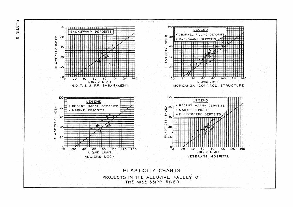
Fluids la &±. Dijfciuwi. IM-1

TECHNICAL MEMORANDUM NO. 3-286

WATERWAYS EXPERIMENT STATION

VICKSBURG, MISSISSIPPI

PRICE $1.00

JUNE 1*49

EC CORPS OF ENGINEERS, U. S. ARMY

MISSISSIPPI RIVER COMMISSION

CORRELATION OF SOIL PROPERTIES

WITH GEOLOGIC INFORMATION

REPORT NO. 1

SIMPLIFICATION OF THE LIQUID

LIMIT TEST PROCEDURE

icgi 1 0 1

a

'5=2?

B

TECHNICAL MEMORANDUM NO. 3-286

WATERWAYS EXPERIMENT STATION

VICKSBURG, M I S S I S S I P P I

MRC-WES 100

JUNE 1949

PROPERTY OF U. S . XJRJST OFFICE CHIEF OF ENGINEERS LIBRARY

CONTENTS

PREFACE i

PAST I: INTRODUCTION 1

PAET II: PRESENT AND PROPOSED LIQUID LIMIT TEST PROCEDURES . . . . 3

Present Test Procedure . . • . . . . . • • 3

Proposed Method of Simplifying Test Procedure . . . . . . . . 3

PAET III: DATA ANALYSIS AND EESULTS . 5

Sources of Data . . 5 Conversion of Data . • • • . . • • • • •• 5 Methods Used in Analysis of Data 6 Nomenclature and Definitions 7 Analysis of Data with Eespect to Geology 9 Analysis of Data with Eespect to Geography 10 Analysis of Eesults • 12 Eecommended Simplified Liquid Limit Procedure . . . . . . . . 19 .

PAET IV: CONCLUSIONS AND EECOMMENDATIONS 21

TABLES 1-3

PLATES 1-22

PREFACE

In a memorandum to the President, Mississippi River Commission,

dated 18 May 19hQ, subject "Special Projects for the Fiscal Year l<&9/!

the Waterways Experiment Station proposed an investigation entitled

"Correlation of Soil Properties with Geologic Information." The project

was approved in the 1st Memo Indorsement dated Ik June 19^8. This report

is the first of a series to be published on this investigation.

The concept upon which this report is based was contributed by

Dr. A. Casagrande, whose valuable assistance is hereby acknowledged.

Acknowledgement is also made to the New Orleans, Vicksburg, and Memphis

Districts, CE, for the use of their laboratory data files which aided

materially in the accomplishment of the investigation.

The study was performed by the Embankment and Foundation Branch

of the Soils Division, Waterways Experiment Station. Engineers connected

with the study were Messrs. W. J. Turnbull, S. J. Johnson, A. A. Maxwell,

S. Pilch and C. D. Burns. This report was prepared by Mr. Pilch.

CORRELATION OF SOIL PROPERTIES WITH GEOLOGIC INFORMATION

SIMPLIFICATION OF THE LIQUID LIMIT TEST PROCEDURE

PART I: INTRODUCTION

1, The general project of correlating soil properties with

geologic information, one phase of which is described in this report,

consists in comparing soil properties with soil types and with their

geologic history and environment in order to determine what correla

tions are possible. If correlations are found to exist, it would be

possible to reduce laboratory testing materially at sites where geo

logic information is available, and to obtain a better understanding

of the behavior and properties of the soils. The purpose of this report

is to present data and analyses from liquid limit tests, and correla

tions which may materially reduce the cost of performing this test.

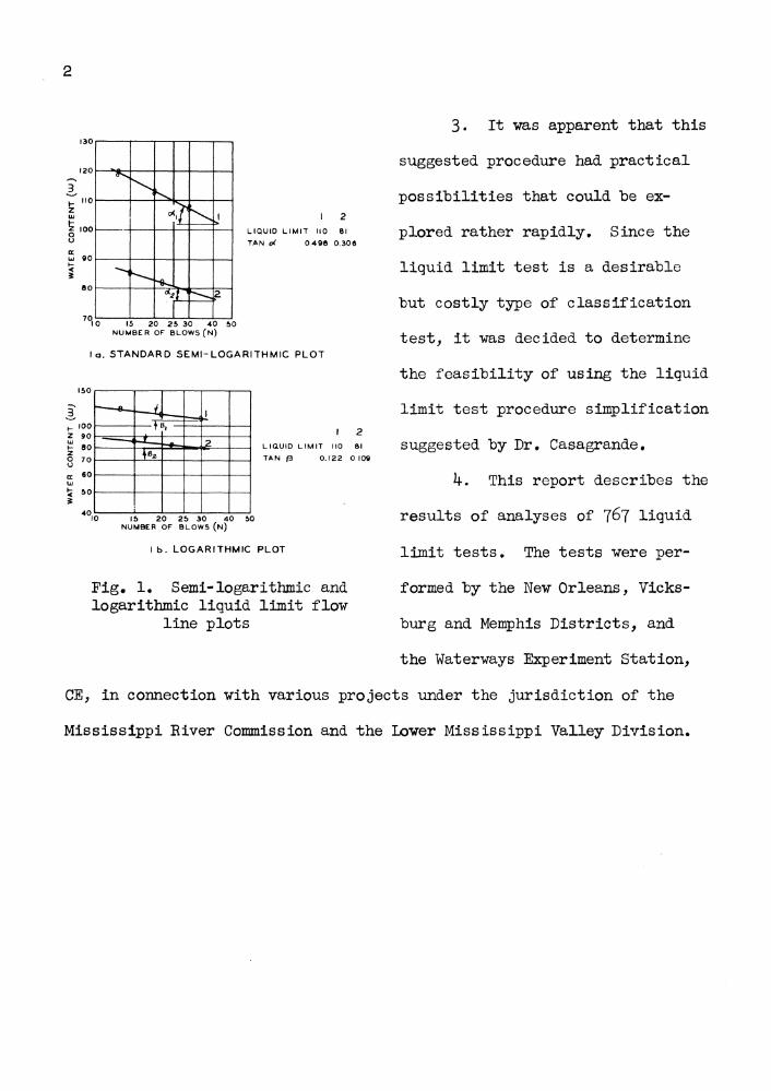
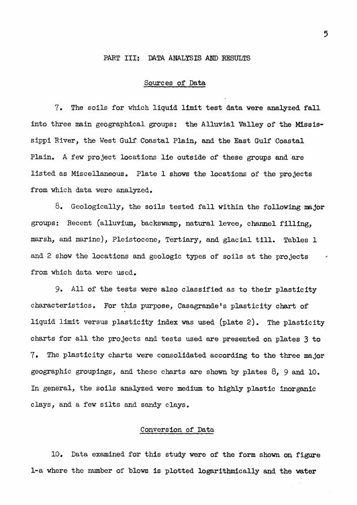
2. Dr. Arthur Casagrande suggested that flow lines determined by

liquid limit tests, plotting both water content and number of blows to a

logarithmic scale, might have a constant slope for soils of the same

geologic origin. The basis for the idea that a logarithmic plot would

give a constant flow-line slope, which the currently-used semilogarith-

mic plot does not, is as follows: On a semilogarithmic plot, flow lines

of higher liquid limit values have, in general, steeper slopes than flow

lines of lower liquid limit values. However, a logarithmic plot reduces

the slope of the higher liquid limit flow lines more than it does the lower,

thus tending to make them equal as is clearly illustrated by figure 1.

2

I 2 LIQUID LIMIT 110 81 TAN oi 0498 0.308

15 20 25 30 40 50 NUMBER OF BLOWS(N)

l a . STANDARD SEMI-LOGARITHMIC PLOT

150

T 100 2 90 UJ

\- 80 I 70

a 60

1 1 a

1

' ?

K

I 2 LIQUID LIMIT 110 81 TAN ^ 0.122 0.109

15 20 25 30 40 50 NUMBER OF BLOWS ( N )

I b. LOGARITHMIC PLOT

Fig. 1, Semi-logarithmic and logarithmic liquid limit flaw

line plots

3. It was apparent that this

suggested procedure had practical

possibilities that could be ex

plored rather rapidly. Since the

liquid limit test is a desirable

but costly type of classification

test, it was decided to determine

the feasibility of using the liquid

limit test procedure simplification

suggested by Dr. Casagrande.

k. This report describes the

results of analyses of 7&7 liquid

limit tests. The tests were per

formed by the New Orleans, Vicks-

burg and Memphis Districts, and

the Waterways Experiment Station,

CE, in connection with various projects under the jurisdiction of the

Mississippi River Commission and the Lower Mississippi Valley Division.

3

PART II: PRESENT AHD PROPOSED LIQUID LIMIT TEST PROCEDURES

Present Test Procedure

5. The Atterberg liquid limit test has been standardized as to

procedure and equipment*. The testing device consists essentially of a

small brass dish which can be raised a distance of one centimeter by a

cam arrangement and allowed to drop on a hard rubber base. The soil

specimen is placed in this dish and a groove is cut in the specimen with

a special grooving tool. The dish is then dropped on the base at a rate

of two drops) or "blows/' per second until a l/2-in. length of the

groove is closed by the flowing together of the soil on each side of the

groove. The liquid limit is the water content of the soil when the

groove closes with 25 blows. It would be too time-consuming to adjust „

the water content of a soil specimen so that the groove would close at

exactly 25 blows. Hence the test is made at several water contents, and

the water content at 25 blows is found by straight-line interpolation on

a graph, plotting the number of blows on a logarithmic scale and water

content on an arithmetic scale; figure 1-a is a typical plot. The line

determined by the plotting of number of blows versus water content is

called a flow line.

Proposed Method of Simplifying Test Procedure

6. It can be seen from figure 1-a that six points have been used

to define a flow line on a semilogarithmic plot. If it can be shown

* Casagrande, A,, "Research on the Atterberg Limits of Soils," Public Roads, Vol. 13, No, 8, October 1932.

k

that the slope of the flow lines for soils in the same geologic formation

is a constant on a logarithmic plot, then the liquid limit can "be deter

mined from one test point for each soil. The point can he plotted on

logarithmic paper, and the flow line, with its predetermined slope, drawn

through this point. The liquid limit would be the water content at the

intersection of the flow line and the 25-blow line. A nomographic chart

could also be made representing the relationship between the liquid limit,

water content, and number of blows for a given flow line slope.

5

PART III: DATA ANALYSIS AMD RESULTS

Sources of Data

7. The soils for which liquid limit test data were analyzed fall

into three main geographical groups: the Alluvial Valley of the Missis

sippi River, the West Gulf Coastal Plain, and the East Gulf Coastal

Plain. A few project locations lie outside of these groups and are

listed as Miscellaneous• Plate 1 shows the locations of the projects

from which data were analyzed,

8. Geologically, the soils tested fall within the following major

groups: Recent (alluvium, "backswamp, natural levee, channel filling,

marsh, and marine), Pleistocene, Tertiary, and glacial till. Tables 1

and 2 show the locations and geologic types of soils at the projects

from which data were used.

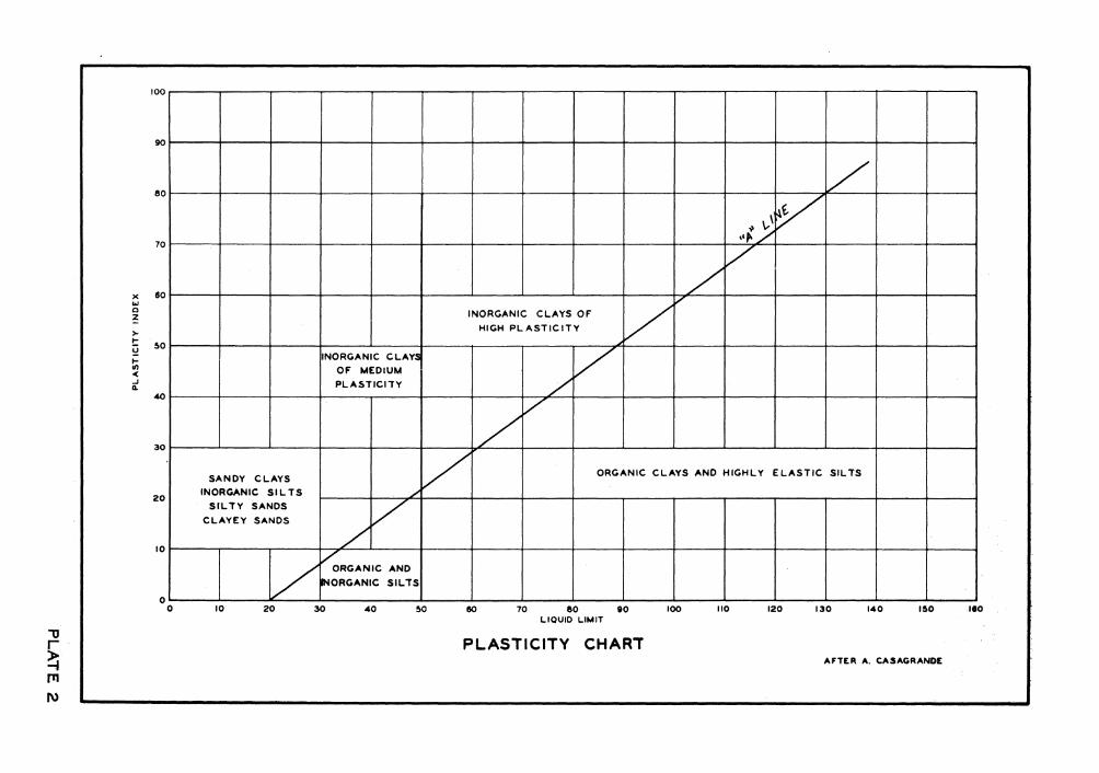
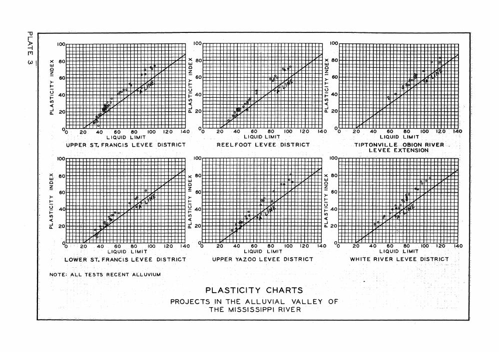
9. All of the tests were also classified as to their plasticity

characteristics. For this purpose, Casagrande's plasticity chart of

liguid limit versus plasticity index was used (plate 2), The plasticity

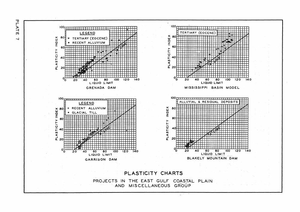
charts for all the projects and tests used are presented on plates 3 to

7» The plasticity charts were consolidated according to the three major

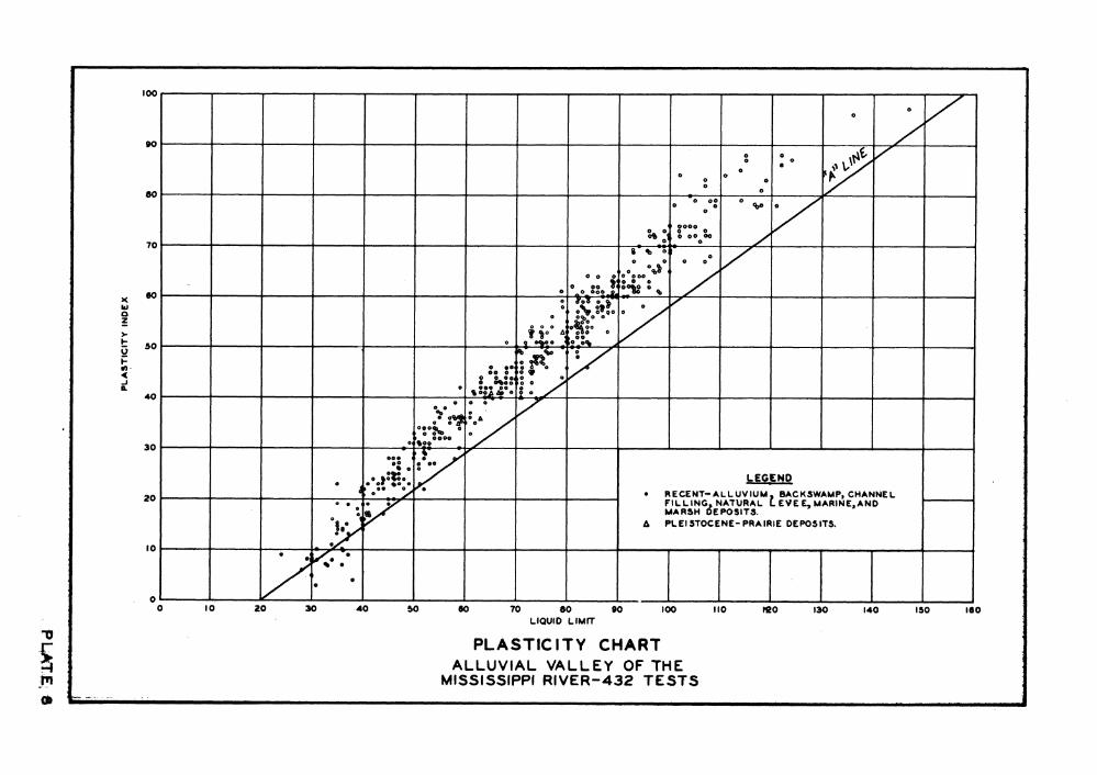
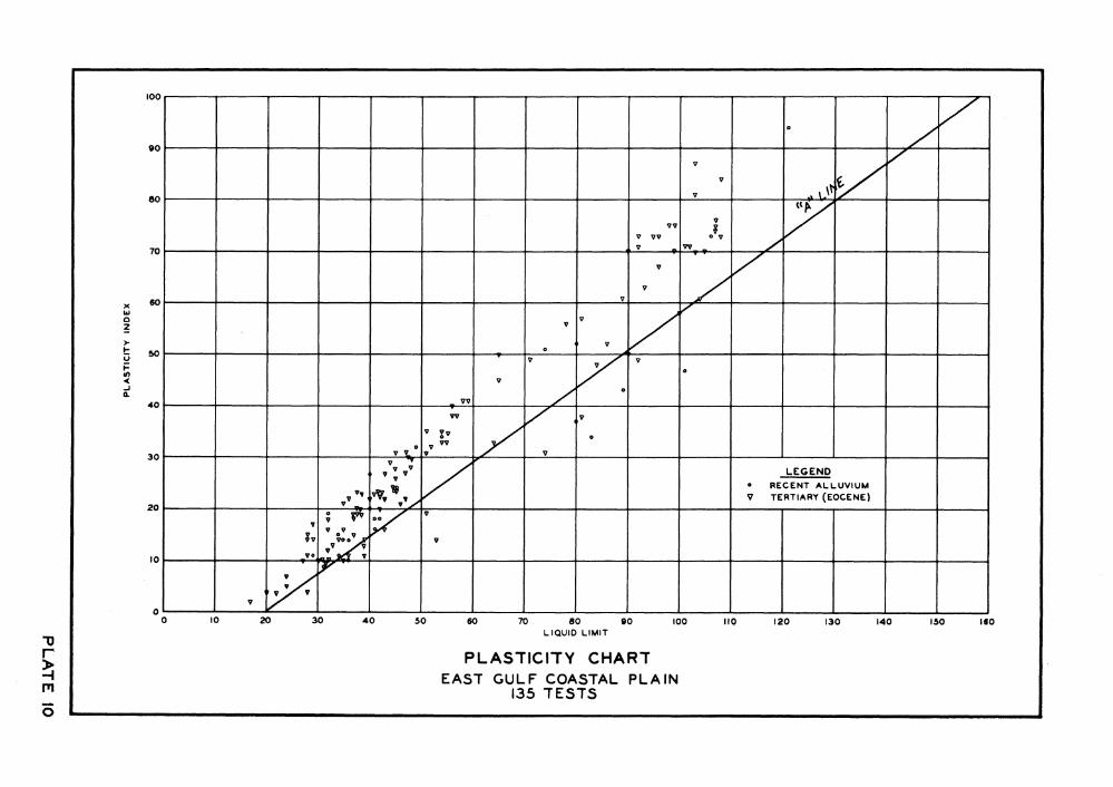
geographic groupings, and these charts are shown "by plates 8, 9 and 10.

In general, the soils analyzed were medium to highly plastic inorganic

clays, and a few silts and sandy clays.

Conversion of Data

10 . Data examined for this study were of the form shown on figure

1-a where the number of blows is plotted logarithmically and the water

6

content arithmetically. To determine the slope of a flow line on a fully

logarithmic plot, it was not necessary to replot the data. The slope of

a flow line on a logarithmic plot can he computed from the semilogarith-

mic plot by the following relationship:

^10

log v1Q - log w 3 0 l o g W30

t a n p a log 30 - log 10 = 0.1+77

where tan p = the slope of the flow line on a logarithmic plot with reference to the horizontal,

v10 a the water content at 10 blows ) from flow line on ) semilogarithmic

w30 = the water content at 30 blows ) plot

Ten and 30 blows were arbitrarily selected for convenience. This method

is not theoretically exact, as a straight line (except a vertical or

horizontal one) on a semilogarithmic plot will not be a straight line

when plotted logarithmically. However, within the range in water con

tents and number of blows of a single flow line for the data utilized,

the variation from a straight line is so small as to be of no conse

quence. Figure 1-b shows data from figure 1-a plotted logarithmically.

Methods Used in Analysis of Data

11. All of the data examined were used except for a few tests in

which it was obvious that the test points were so erratic that a reason

ably precise flow line could not be determined. The data were also

limited to tests for which the liquid limit was less than 150.

12. It should be noted that liquid limit test results depend to a

considerable extent on individual technique; and since the tests analyzed

were performed by many technicians, some degree of control over the data

7

was lost. However, it is "believed that the methods used in the analysis

give results which accommodate a large part of the variations in the data

due to differences in technique,

13. The large number of tests utilized made it necessary to adopt

methods to present the data in a concise, yet complete form. To fill

this need, statistical methods were used in analysis of the data and

presentation of results. The statistical methods and nomenclature used

are those recommended by the American Society for Testing Materials.*

Nomenclature and Definitions

Ik. For purposes of clarity, the nomenclature and definitions used

in this study are given below:

tan P , tan p ^> * a n (3 v * a n 3 * observed values of

tan (3 ; slope of flow line on a logarithmic plot.

n: the number of observations,

f: the frequency, the number of observations for a given

value, or . interval, of tan p .

tan p : the arithmetic mean or average, referred to as the

mean in this report,

n

5 tan Pi * n tan p =s -i5± , where ^ tan p . means the

n i=l

sum of all the values of tan p from tan 3 1 to

tan p , inclusive.

* A.S.T.M. Manual on "Presentation of Data," April 19^5 (reprint).

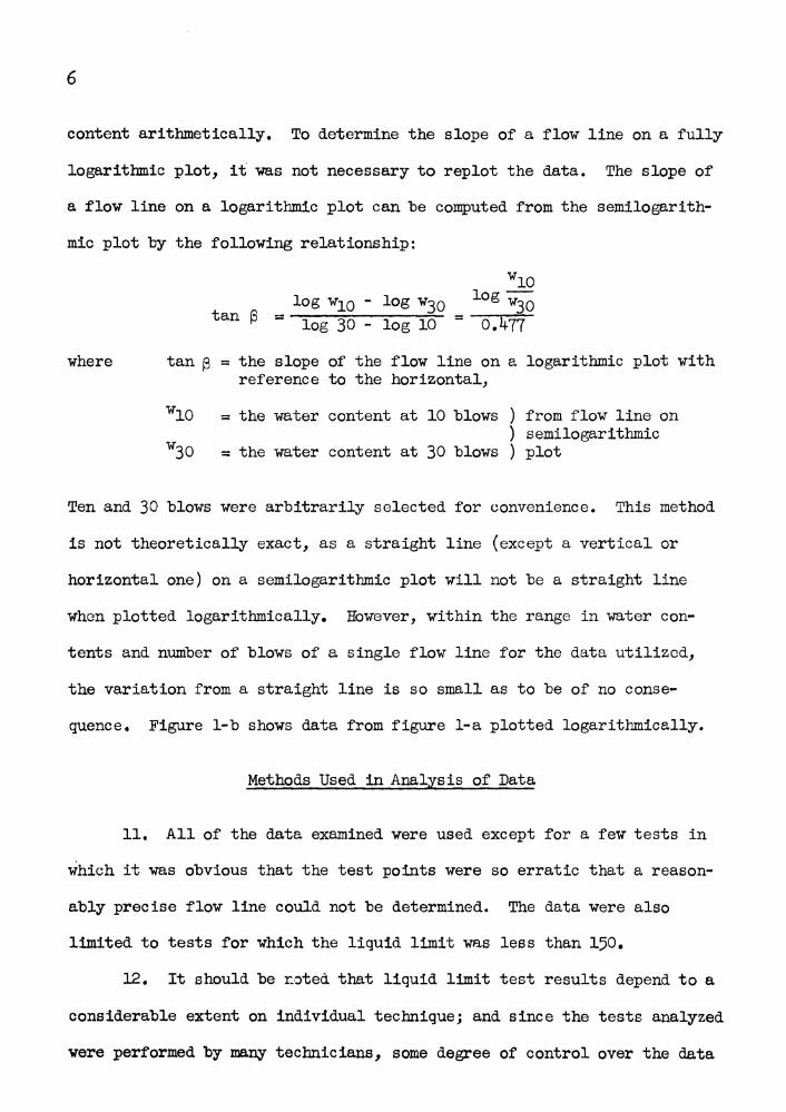
a : the standard deviation, the moat significant and efficient

measure of dispersion of data about a mean* For a nor

mal frequency curve, the mean plus and minus the stand

ard deviation includes 68.3 per cent of the total

number of observations,

T[

a =

(tan p. - tan p )

n

v: the coefficient of variation, a measure of relative disper

sion of data about a mean. Useful in comparing distrib

utions with different means,

v# = -zzzzzr* x 10° •

tan (3

k: Hazen's coefficient of skewness, a measure of the non-

symmetry of a distribution about a mean, A positive

value of k generally means that the observed values

extend farther to the right of the mean than to the

left; a negative value of k, vice versa. For a sym

metrical normal frequency curve k =: zero.

*L o ^> (tan (3 . - tan 3 )-*

k . & L n o J

Normal frequency curve: the curve defined by the equation

(tan B ) 2

ay 2 n

It is the familiar bell-shaped curve and represents a

9

theoretically correct frequency distribution (see

figure 2, page 10).

Analysis of Data with Bespect to Geology

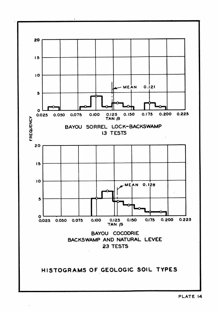
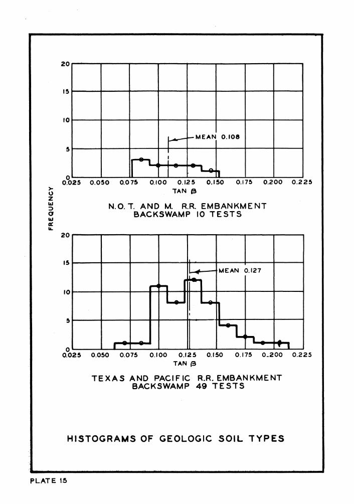
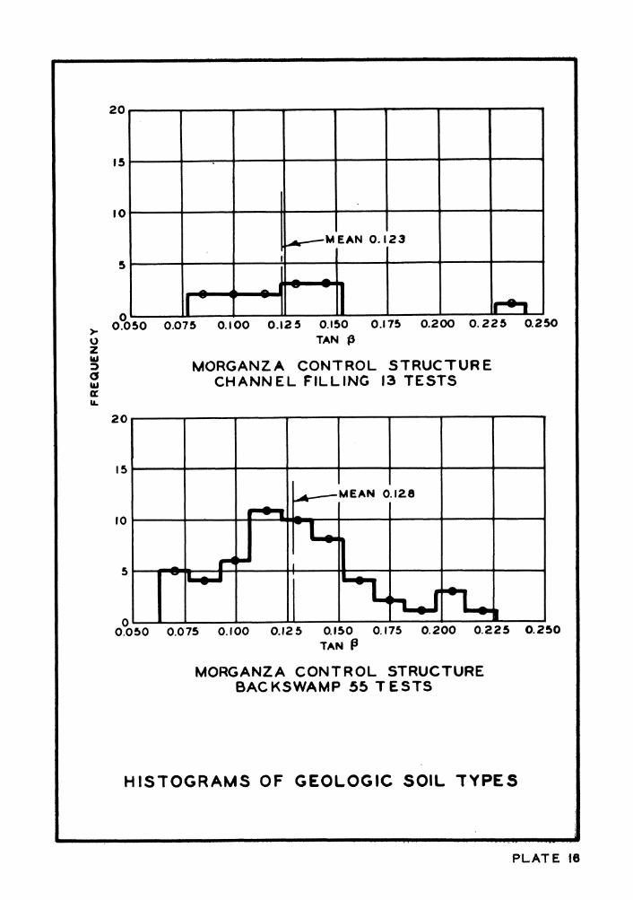
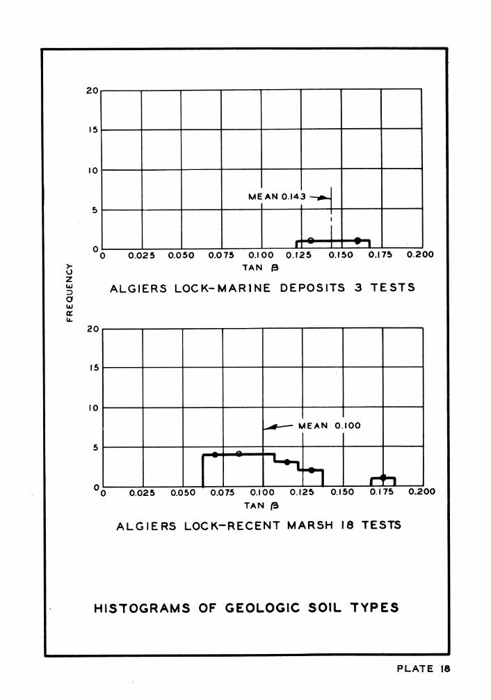
15. The individual values of tan (3 were computed to the nearest

thousandth "by the method discussed in paragraph 10. To show graphically

the distribution of tan (3 for each geologic soil type within the proj

ects, frequency histograms were plotted (plates 11-22). The frequency

histograms have as their abscissas values of tan 3 grouped in classes

with intervals of 15 thousandths, and as their ordinates, the frequency.

16. The mean tan (3 for each project was computed by the equation

in paragraph 14-. These means are listed in tables 1 and 2 and are

plotted on the histograms; the means from all the various geologic types

and projects range from 0.094 (White River Levee District, Recent

alluvium, 25 tests) to 0.1^3 (Algiers Lock, Recent marine, 3 tests), a

range of O.Olj-9. The range of tan (3 within each geologic soil type

averages about 0.1; maximum range O.168 (Grenada Dam Tertiary, Eocene),

minimum range 0.050 (Greenwood Protection Levee, Recent alluvium). The

range of tan 3 within soil groups of the same geologic classification

is greater than the range of the means of all geologic soil types. Also,

an inspection of the means in tables 1 and 2 shows no tendency for each

geologic type to group itself about a single mean tan 3 • From these

observations it appears that, for the soil types studied, the slope of

the flow line is not directly related to the geologic classification of

the soil.

10

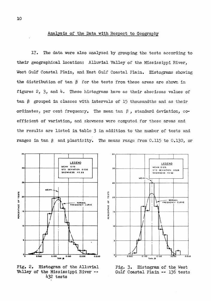
Analysis of the Data with Respect to Geography

17. The data were also analyzed by grouping the tests according to

their geographical location: Alluvial Valley of the Mississippi River,

West Gulf Coastal Plain, and East Gulf Coastal Plain. Histograms shoving

the distribution of tan (3 for the tests from these areas are shown in

fig ires 2, 3, and 4. These histograms have as their abscissas values of

tan (3 grouped in classes with intervals of 15 thousandths and as their

ordinates, per cent frequency. The mean tan (3 , standard deviation, co

efficient of variation, and skewness were computed for these areas and

the results are listed in table 3 in addition to the number of tests and

ranges in tan (3 and plasticity. The means range from 0.115 to 0.130, or

J /

L

V

LEGEND

MEAN 0.116 5TD DEVIATION 0 032

SKEWNESS +0 55

^ \

\

NORMAL FREQUENCY CURVE

V

0.100 0.150 TAN 0

Fig. 2. Histogram of the Al luvia l Valley of the Mississippi River - -

if32 t e s t s

Fig. 3. Histogram of the West Gulf Coastal Plain — 136 tests

11

1 1 LEGEND

MEAN 0 130 STD SKEW

DEVIATION NESS + 0 . 4

0.035 4

MEA

/

3 -i

r

Ji i \ * r - N 0

7 F R E Q U E RMAL NCY CURVE

1 K / \

*s / U^

^ 0 100 0 150

TAN (3

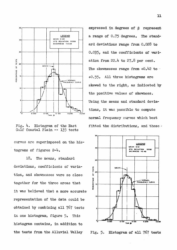
Fig, k* Histogram of the East Gulf Coastal Plain -- 135 tests

expressed in degrees of p represent

a range of 0.75 degrees. The stand

ard deviations range from 0,028 to

0.035, and the coefficients of vari

ation from 22.4 to 27.8 per cent.

The skewnesses range from +0.42 to -

+0.55# All three histograms are

skewed to the right, as indicated by

the positive values of skewness.

Using the means and standard devia

tions, it was possible to compute

normal frequency curves which best

fitted the distributions, and these -

curves are superimposed on the his

tograms of figures 2-4.

18. The means, standard

deviations, coefficients of varia

tion, and skewnesses were so close

together for the three areas that

it was believed that a more accurate

representation of the data could be

obtained by combining all 7^7 tests

in one histogram, figure 5« This

histogram contains, in addition to

the tests from the Alluvial Valley

0.100 0 1 TAN 0

50 0.200

Fig. 5. Histogram of a l l 767 t e s t s

12

of the Mississippi Eiver and the East and West Gulf Coastal Plains, the

tests from the two projects outside these three general areas: Garrison

Dam, N#D., mean 0,123, and Blakely Mountain Dam, Ark., mean 0.123. The

mean for all 767 tests is 0.121, the standard deviation 0.032, the coef

ficient of variation 26.4 per cent, and the skewness +0.42 (table 3).

The normal frequency curve was computed and superimposed on the histogram,

figure 5» This histogram "best fits its normal frequency curve, as a com

parison with the histograms of figures 2-4 shows. This was to "be expected

because of the large number of tests used in its development. The fact

that the skewness coefficient is lower for the histogram of all the tests

than for any of the three principal geographic areas is also indicative

of a better fit to the normal frequency curve.

Analysis of Results

Equation for the liquid limit on a logarithmic plot

19. It can be shown that the value for the liquid limit using a

logarithmic plot and one point on the flow line is determined by the

equation:

/ H \ tan 3

where LL = liquid limit,

VJJ a water content at N blows from the liquid limit device,

tan p =» slope of the flow line on a logarithmic plot.

13

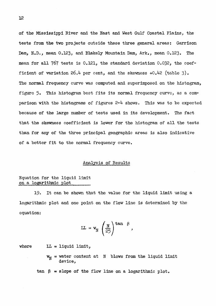
Effect of variations in the slope of the flow line on the value of the liquid limit

20. The method of differentials is applicable to measuring the

effect of variations in tan (3 on the value of the liquid limit. The

expression for per cent change in the liquid limit is derived as follows:

tan 3

( .T \ tan 3 N

JLJ x l n | x d (tan 3 )

(in refers to logarithms to the base e)

and —:*=—*• a l n ^ x d (tan (3 ).

This may also be written as: A (LL) $ = In iL x A (tan 3 ) x 100, LL F 25

in which — = ^ — * $ is the per cent change in the liquid limit for a change

A (tan 3 ) in the slope of the flow line on a logarithmic plot. An in

spection of this equation shows that the per cent change in the liquid

limit is independent of the actual values of both the liquid limit and

the slope of the flow line. It depends only on a given variation in the

slope of the flow line and the number of blows. The above equation is

plotted on figure 6 (page Ik) for various values of N and A (tan 3 ).

Comparison of mean slopes

21. The pertinent results determined for the geographical areas

are summarized on the following page (from table 3):

14

J 7 J 7 A ( LL ) N 1 %= Ih X ATAN3 X 100

25 1 - LL

) N 1 %= Ih X ATAN3 X 100 25

1 8

o _ > 5 5 o

Y 7 ' - j io .A—

V 7 * • &/ L

4 Z V \ 1 o

V

o Ul > o V

&

o

V o-S £^ z 3

< \X / ^ I

o > ^

2 »-z v 0

fc T

UJ O i ^J

fc J O^i^-

cr 1 ^J r r^ 5n? & ««« = o01

n 1 rSi ^ . htf^

& 1

10 20 25 30 40 NUMBER OF BLOWS (N)

50 60

Fig. 6. Per cent change in liquid limit vs number of blows for changes in tan (3

No. Mean Standard Coefficient of Skew-Tests tan (3 Deviation Variation (jo) ness

Alluvial Valley of the Mississippi Eiver

^32 0.115 0,032 27.8 +0.55

West Gulf Coastal Plain 136 0.125 0.028 22.4 +0.52

East Gulf Coastal Plain 135 0.130 0.035 26.9 +0.44

Al l t e s t s (including 64 from the Miscellaneous group)

767 0.121 0.032 26.4 +0.42

The magnitude of the differences between the mean for all tests and for

the three principal geographic areas is best understood by reference to

the change in the liquid limit due to these variations. The mean of all

the tests, 0,121, differs from the mean of the Mississippi Eiver Alluvial

Valley, 0,115, by 0.006. This would make a difference in the liquid

limit determination of 0.3 per cent, using 15 blows, figure 6. This

15

illustrates that the differences between the means in the above table are

of an extremely small magnitude when referred to the differences that

they would make in computing liquid limits. The means of the West Gulf

Coastal Plain and the East Gulf Coastal Plain, although from relatively

small numbers of tests, differ from the mean of 0.121 by 0.00*4. and 0.009,

respectively. The dispersion of data about the four individual means is

least for the West Gulf Coastal Plain, as is seen by an inspection of the

coefficients of variation and standard deviations* This is not necessar

ily conclusive, however, as the smaller number of tests involved means a

greater probability for a narrower range in tan (3 , which in turn results

in a smaller coefficient of variation. For practical purposes the meas

ures of dispersion and skewness are essentially the same for all group

ings. Based on the above factors it

is believed that the histogram of

all the tests, figure 5, with its

mean of 0.121 best represents all

the data studied, and the remainder

of this report will be referred to

this value.

Per cent error involved in liquid limit determinations^

22. The histogram and normal

frequency curve for all 767 tests

were plotted on arithmetic probabil

ity graph paper, figure 7. The ordi-

nates of this graph are so spaced

< 8 5 0

> ui < » 0 0 o < 8 0 0 I t-

tf> 7 0 0 <n

-i ©0 0

z 5 0 0 < h 40 0 X g 3 0 0

£ 2 0 0 Ui

O 10 0

UJ 5 0

/ o

/ f • LEGEND

MEAN 0 121

STD DEVIATION (0) 0 0 3 2

S K E W N E S S + 0 . 4 2 ' t

i FREC

NOR UENC

rfAL Y CU RVE -

o 1 . /

Ml A N - H / I t

A / f I

I o

/ I

; - - I % 1 / | \

i

J f t

-a I

F * 2 o

i '| 1 q

| /

/ I 0 0 5 0 0.100 0.150 0 .200 0 . 2 5 0 O.KK) TAN (%

Pig. 7. Arithmetic cumulative frequency curve — 7^7 tests

16

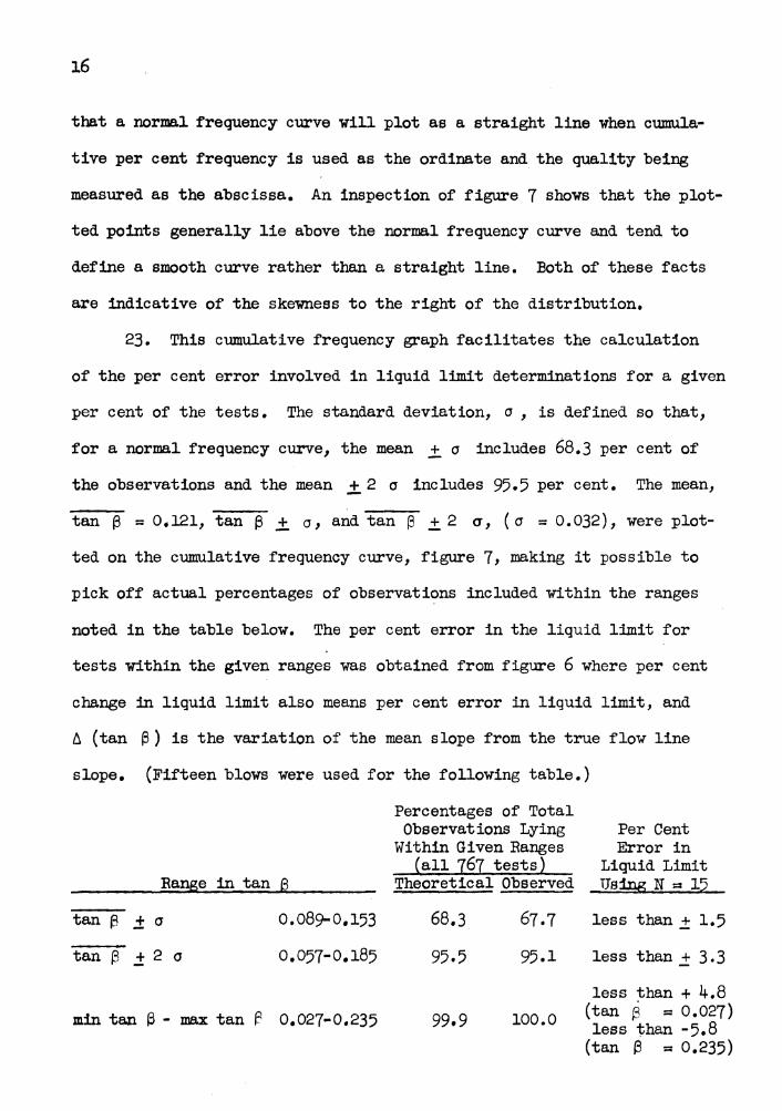
that a normal frequency curve will plot as a straight line when cumula

tive per cent frequency is used as the ordinate and the quality being

measured as the abscissa. An inspection of figure 7 shows that the plot

ted points generally lie above the normal frequency curve and tend to

define a smooth curve rather than a straight line. Both of these facts

are indicative of the skewness to the right of the distribution,

23. This cumulative frequency graph facilitates the calculation

of the per cent error involved in liquid limit determinations for a given

per cent of the tests* The standard deviation, o , is defined so that,

for a normal frequency curve, the mean JH 0 includes 68.3 per cent of

the observations and the mean + 2 a includes 95*5 per cent. The mean,

tan (3 ss 0.121, tan (3 ± a, and tan (3 ± 2 a, (a = 0.032), were plot

ted on the cumulative frequency curve, figure 7> making it possible to

pick off actual percentages of observations included within the ranges

noted in the table below. The per cent error in the liquid limit for

tests within the given ranges was obtained from figure 6 where per cent

change in liquid limit also means per cent error in liquid limit, and

A (tan (3 ) is the variation of the mean slope from the true flow line

slope. (Fifteen blows were used for the following table.)

Percentages of Total

Observations Lying Per Cent Within Given Ranges Error in

(all 767 tests) Liquid Limit Bange in tan 6 Theoretical Observed TJs

tan p + a 0.089-0.153

tan (3 + 2 o 0.057-0.185

min tan (3 - max tan (? 0.027-0.235

68.3 67.7

95.5 95.1

99*9 100.0

less than + 1.5

less than + 3«3

less than + k.8 (tan {3 « 0.027) less than -5»8 (tan (3 » 0.235)

17

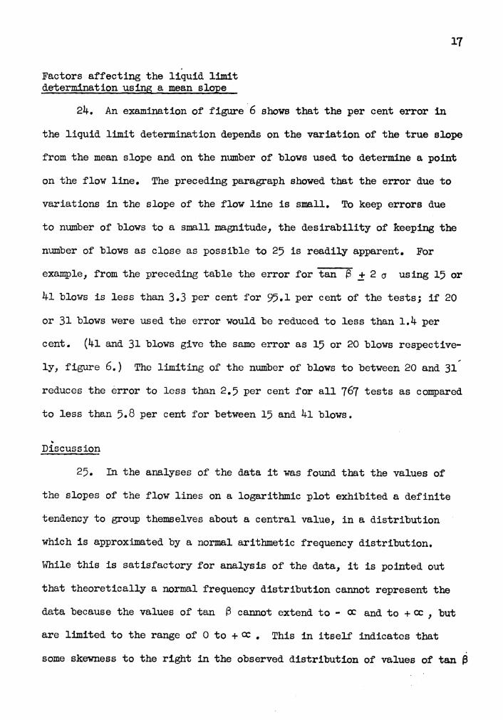
Factors affecting the liquid limit determination using a mean slope

2k. An examination of figure 6 shows that the per cent error in

the liquid limit determination depends on the variation of the true slope

from the mean slope and on the number of "blows used to determine a point

on the flow line. The preceding paragraph showed that the error due to

variations in the slope of the flow line is small* To keep errors due

to number of blows to a small magnitude, the desirability of keeping the

number of blows as close as possible to 25 is readily apparent. For

example, from the preceding table the error for tan 3 + 2 <j using 15 or

kl blows is less than 3.3 per cent for 95.1 per cent of the tests; if 20

or 31 blows were used the error would be reduced to less than 1.1*. per

cent, (kl and 31 blows give the same error as 15 or 20 blows respective

ly, figure 6.) The limiting of the number of blows to between 20 and 31

reduces the error to less than 2.5 per cent for all 767 tests as compared

to less than 5*8 per cent for between 15 and kl blows.

Discussion

25. In the analyses of the data it was found that the values of

the slopes of the flow lines on a logarithmic plot exhibited a definite

tendency to group themselves about a central value, in a distribution

which is approximated by a normal arithmetic frequency distribution.

While this is satisfactory for analysis of the data, it is pointed out

that theoretically a normal frequency distribution cannot represent the

data because the values of tan 3 cannot extend to - oc and to + cc , but

are limited to the range of 0 to + oc # This in itself indicates that

some skewness to the right in the observed distribution of values of tan (3

18

< 95.0

> Ui J «00 < Z 8 0 0

*~ 70.0 <n m * «0.0

• so.o z < 400

X *" 30.0

* <0 20.0 S 15.0 u. 10.0 o

i / -

1

1 t. I _ zt _ ___7_ .

p -: z::j :

i

—t- -_y____ .

,,

/

6.010 0.020 0.030 0.05& 0.100 ai50 0.200 0.300 TAN 3

Fig. 8. Logarithmic cumulative frequency curve — 7^7 tests

should be expected, and it is likely

that the distribution may be better

approximated by a logarithmically

normal frequency distribution* As a

check on this possibility, the data

shown on figure 7 were plotted on

logarithmic probability paper, fig

ure 8 (identical to the arithmetic

probability paper except for the

substitution of a logarithmic scale

for the arithmetic one). On this

type of plot all the points, except

those for tan 3 equal 0.025 and

0.0^0, lie on a straight line, in

dicating that the distribution of values of tan 3 is logarithmically

normal rather than arithmetically normal. However, for the purpose of

this investigation it was considered that an arithmetically normal fre

quency distribution could be used.

26. The observed variations of tan 3 from the mean may *be due to

a natural distribution of tan 3 as a property of the soils studied.

However, the variations from the mean may also be due, in part, to errors

involved in performing the tests rather than to any property of the soil

itself. All technicians in the soils laboratory of the Waterways Experi

ment Station are, at intervals, requested to perform the liquid limit

test on the same material. Study of the results so obtained indicates a

variation in values of both the liquid limit and tan 3 , with a grouping

19

of the test results in such a way as to suggest that they follow a natu

ral error distribution; a distribution of the same form as the normal

frequency curve. However, this report is not concerned with which

explanation best describes the observed variations, since the variations

themselves are of limited significance.

27. The results obtained from the analyses described herein are

not intended to apply to soils other than those tested, and no generali

zation to other soils is made. As regards the soils of the Alluvial

Valley of the Mississippi River and the East and West Gulf Coastal Plains,

however, sufficient tests have been analyzed to warrant consideration of

a simplified liquid limit test procedure for work in the laboratories of

the Mississippi Eiver Commission and Lower Mississippi Valley Division.

For soils from other areas the procedure may be just as applicable, but

the values of tan (3 should first be determined by preliminary tests. To

take full advantage of the fact that, for the soils studied, the disper

sion of the flow line slopes is of such small magnitude that errors aris

ing from the use of a mean slope are negligible, the liquid limit test

procedure outlined in the following paragraphs is presented.

Recommended Simplified Liquid Limit Procedure

28. The simplified liquid limit procedure is as follows:

a. The test should be run in a humid room if the air is dry* Mix the soil to be tested with water to a consistency as close to the liquid limit as possible, A technician can, with experience, judge this very closely. Extreme care should be taken in the mixing to obtain a uniform water content throughout the sample,

b. Operate the liquid limit device and determine the number of blows necessary to close a l/2-in. length of the groove.

20

Take a 15-20 gm wet weight sample at the closed groove for a water content determination. Water content weights should be accurate to 0.01 gm.

c. Add enough soil paste at the water content of step a to replace that removed, and remix the soil slightly in the liquid limit cup without the addition of water. Eegroove and operate the device again. The number of blows necessary to close l/2 in. of the groove should either be the same as before or not more than two blows different, (if it is not, it is a sign of insufficient mixing in step a, and the entire procedure should be repeated.) Take another sample at the closed groove for a water content dot er minat ion •

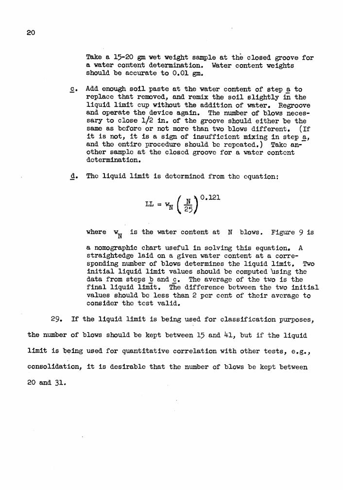
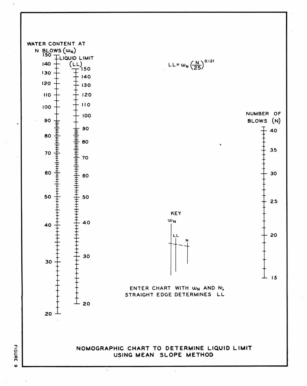
d. The liquid limit is determined from the equation:

where w is the water content at N blows. Figure 9 is

a nomographic chart useful in solving this equation, A straightedge laid on a given water content at a corresponding number of blows determines the liquid limit. Two initial liquid limit values should be computed using the data from steps b and c. The average of the two is the final liquid limit. The difference between the two initial values should be less than 2 per cent of their average to consider the test valid.

29. If the liquid limit is being used for classification purposes,

the number of blows should be kept between 15 and kl, but if the liquid

limit is being used for quantitative correlation with other tests, e.g.,

consolidation, it is desirable that the number of blows be kept between

20 and 31.

WATER CONTENT AT N BLOWS ( U J N )

150 -T-—LIQUID LIMIT 140 —

130 4 -

120

no -h

100

90 - -

80 -EE-

70 -jr-

60 - -

50

4 0 —

30 —

20 - 1 -

CLL). 150

- - 140 = - 130

-+- 120

110

- h 100

4§- 80

iF 70

iz 6 0

- - 50

— 4 0

3 0

-L- 2 0

LL=u,N(-iL) 0.121

NUMBER OF

BLOWS (N)

4 0

3 5

— 30

— 2 5

KEY

LL - - 20 N

-L- 15

ENTER CHART WITH UJN AND N-, STRAIGHT EDGE DETERMINES LL

NOMOGRAPHIC CHART TO DETERMINE LIQUID L IMIT USING MEAN SLOPE METHOD

21

PAET IV: CONCLUSIONS AND RECOMMENDATIONS

30. Based on the data and analyses presented in this report, the

following conclusions are warranted for the soils studied — namely,

medium to highly plastic inorganic clays with liquid limits less than 150

from the Alluvial Valley of the Mississippi River and the East and West

Gulf Coastal Plain areas,

a. The slopes of liquid limit flow lines, when plotted to a logarithmic scale, tend to group around a central value which appears to be independent of soil type and geologic classification.

b. The variations of the slopes of the flow lines for the soils studied, without regard to geologic origin, satisfactorily approximate a normal frequency distribution. This result makes it possible to use the simplified liquid limit procedure.

c. Liquid limits computed using a mean flow line slope of 0.121 and one liquid limit test point give results well within the accuracy required in normal work.

d. It is recommended that the simplified liquid limit procedure described in paragraphs 28-29 be adopted for soils from the Alluvial Valley of the Mississippi River and the East and West Gulf Coastal Plain areas. This procedure will result in a substantial reduction in the cost of liquid limit determinations.

TABLES

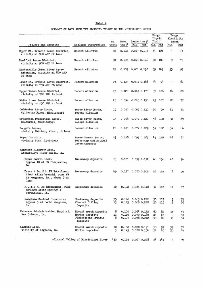
Table 1

SUMMARY OF DATA. FROM THE ALLUVIAL VALLEY OF THE MISSISSIPPI RIVER

Range Range Liquid Plasticity

No. Mean Range tan <3 Limit Index Project and Location Geologic Description Tests tan 3 Min Max Min Max Min Max

Upper St. Francis Levee District, Recent alluvium 40 0.112 0.027 0.193 33 104 4 74 vicinity mi 900 AHP rt "bank

Reelfoot Levee District, Recent alluvium 30 0.122 0.071 O..I76 30 102 9 73 vicinity mi 900 AHP It bank

Tiptonville-Obion River Levee Recent alluvium 25 0.107 0.06l 0.130 59 147 35 97 Extension, vicinity mi 850 AHP It bank

Lower St. Francis Levee District, Recent alluvium 25 0.123 0.071 0.186 34 94 7 62 vicinity mi 750 AHP rt bank

Upper Yazoo Levee District, Recent alluvium 25 0.122 O.O63 O.I76 35 106 14 80 vicinity mi 700 AHP It bank

White River Levee District, Recent alluvium 25 0.094 O.O65 0.130 43 107 22 77 vicinity mi 65O AHP rt bank

Cold-water River Leyee, Yazoo River Basin, 15 0.097 O.O69 0.130 50 99 31 73 Coldwater River, Mississippi recent alluvium

Greenwood Protection Levee, Yazoo River Basin, 13 O.O98 0.072 0.122 56 100 32 69 Greenwood, Mississippi recent alluvium

Bougere Levee, Recent alluvium 22 0.101 0.074 0.129 59 122 34 86 vicinity Natchez, Miss., rt bank

Bayou Cocodrie, Lower Tensas Basin, 23 0.128 0.097 O.I85 47 115 26 87 vicinity Shaw, Louisiana backswamp and natural

levee deposits

Morganza Floodway Area, Atchafalaya River Basin, La.

Bayou Sorrel Lock, Backswamp deposits 13 0.121 0.037 0.192 66 136 40 96 approx 10 mi SW Plaquemine, La.

Texas & Pacific RR Embankment Backswamp deposits 49 0.127 0.070 0.202 28 122 6 90 (Port Allen branch), runs NW fm Morganza, La., about 5 mi long

N.0.T.& M. RR Embankment, runs Backswamp deposits 10 0.108 0.084 0.148 34 103 11 67 between Krotz Springs & "Cortableau, La.

Morganza Control Structure, Backswamp deposits 55 0.128 O.O63 0.222 30 117 3 79 approx 5 mi north Morganza, Channel filling 13 0.123 0.080 0.228 30 115 5 88 La. deposits

Veterans Administration Hospital, Recent marsh deposits 8 0.109 0.084 0.132 60 82 35 54 New Orleans, La. Marine deposits 12 0.115 0.070 0.180 24 83 9 52

Pleistocene-Prairie 8 0.104 O.O38 0.212 59 82 35 54 deposits

Algiers Lock, Recent marsh deposits 18 0.100 0.070 0.171 58 99 37 71 vicinity of Algiers, La. Marine deposits 3 0.143 0.128 0.154 54 66 38 44

Alluvial Valley of Mississippi River 432 0.115 0.027 0.228 24 147 3 97

Table 2

SUMMARY OF DATA FROM THE EAST AND WEST GULF COASTAL PLAINS "AMD MISCELLANEOUS GROUP

Project and Location

Texarkana Dam, Sulphur River, vicinity Texarkana, Ark.

Wallace Lake Dam, Red River, approx 15 mi south Shreveport, La.

Red River Lateral Canal, vicinity of Marksville, La.

Schooner Bayou, approx 18 mi south Abbeville, La.

Range Range Liquid Plasticity

No. Mean Range tan P Limit Index Geologic Description Tests tan ft Min Max Min Max Min Max

WEST GULF COASTAL PLAIN

106 0.122 0.073 O.I82 25 99 9 Pie istocene-Terrace deposits

Red River Valley, recent alluvium

Red River Valley, recent alluvium

Pleis tocene-Prair ie deposits

13 0.127 0.09^ 0.170 57 85 33

10 0.120 0.07^ 0.212 30 Jk 11

7 0.133 O.O65 0.210 31 83 5

West Gulf Coastal Plain 136 0.125 O.O65 0.212 25 99

16

59

k8

kQ

16

Grenada Dam,, v i c in i t y Grenada, Miss.

Mississippi River Basin Model, Clinton, Miss.

EAST GULF COASTAL PLAIN

Yalobusha River Valley Ter t iary (Eocene) 69 0.133 O.067 0.235 17 100 Recent alluvium 25 0.129 O.O69 0.192 29 121

Ter t iary (Eocene)

East Gulf Coastal Plain

kl 0.128 0.073 0.179 32 108

135 0.130 O.O65 0.235 17 121

73 9k

16 87

.*

Garrison Dam, vicinity Garrison, N. D.

Blakely Mountain Dam, 10 mi NW Hot Springs, Ark,

MISCELLANEOUS

Missouri River Valley Recent alluvium Glacial till

k2 0.121 0.063 0.197 30 99 3 76 7 0.138 0.100 0.207 26 ko 10 22

Average k9 0.123

Ouachita River Valley Residual and Alluvial 15

Miscellaneous 6k

0.123 0.074 0.151 20

0.123 0.063 0.207 20

33

99

16

76

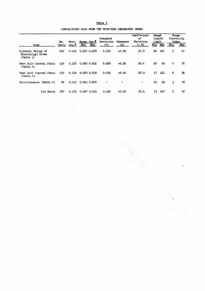
Table 3

CONSOLIDATED DATA EROMt THE P^OTOim GEOGRAPHIC AREAS

Coefficient Range Range Standard of Liquid Plasticity-

No. Mean Range tan ft Deviation Skevness Variation Limit Index Area Tests tan f Min Max (a) (is) (v 4) Min- Max, Klin Max

Alluvial Valley of ^32 0.115 0.027 0.228 0.032 +0.55 27.8 2k lVf 3 97 Mississippi River (Table l)

West Gulf Coastal Plain 136 0.125 O.O65 0.212 0.028 +0.52 (Table 2)

East Gulf Coastal Plain 135 0.130 O.O65 0.235 0.035 + 0 . ^ (Table 2).

Miscellaneous (Table 2) 6k 0.123 O.O63 0.207 - -

All Tests 767 0.121 0.027 0.235 0.032 +0.1*2

22 A 25 99 5 16

26.9 IT 121 2 <*

- 20 99 3 16

26.k IT ihl 2 9T

PLATES

32° 3 , c 30°

^7777-777-' • / • • • - / / / / / • '

^C-A////Xv> ' ' AA/AA _ 37c

36«

35'

sr

A L L U V I A L V A L L E Y OF MISSISSIPPI RIVER

I - U P P E R ST FRANCIS LD 2 - R E E L F O O T LO 3 - T IPTONVILLE OBION R. LEVEE EXT. 4 - LOWER ST FRANCIS LD 5 - UPPER YAZOO LD 6 - WHITE RIVER LD 7 - COLDWATER R. LEVEE 8 - GREENWOOD PROTECTION LEVEE 9 - BOUGERE LEVEE

1 0 - BAYOU COCODRIE 1 1 - MORGANZA CONTROL STRUCTURE 1 2 - T . i R R.R. EMBANKMENT 1 3 - NOTM R.R. EMBANKMENT 14 - BAYOU SORREL LOCK 1 5 - V.A. HOSPITAL 1 6 - ALGIERS LOCK

WEST GULF COASTAL PLAIN

1 7 - TEXARKANA DAM 1 8 - WALLACE LAKE DAM 1 9 - RED RIVER LATERAL CANAL

2 0 - SCHOONER BAYOU

EAST GULF COASTAL P L A I N

21 - GRENADA DAM 2 2 - MISS. R. BASIN MODEL

MISCELLANEOUS GARRISON DAM N.D.

2 3 - BLAKELY MOUNTAIN DAM

A ix / ' l / k p l a r Bluffy

Ac;/

/A/// 'A// Cape Gira

A •Golccndal

rard«

?bes- / ,

fcdvance/

Commerced

Charleston o

^MoundCityl tCAlRO

Wickliffe Paducah

V-A loomfield 0 ^ V/ Morehouse

°Sikeston r$\

[New Madrid l°Malden |

/ i

Portagevilleo )\ (

/) rS' ' Caruthersville ^ ~

J*7s ''

\r%

« Columbus

o •Ob'*

. . A Jonesborol

btytheville<

i i

Osceola p((

5 Marked Tree

jltori

/

Lake^ W / / / / V /

V/A//A/A /

T E N N / / V / /

/ /

/

^chL'/

'/<z&y

V>DesAix / ,

/ZAA RiVi & * '

. L I T T L E ROCK

/ / /

kV

«v Mariar»n»2^ 7°Clarendor!

«

• /

/ / vZr

/

Stuttgart o Marvel^

, / ' BLUFF A ^

' / , V>

A,

A

A

/ .

Helena^

'ito \Mark« o(

'Clarksdale

' . - V .

'A /.rt

A, /

X n /

'/•.

/ /.

/ ' A / A

* / , A

'S Z*o /

/ / / .

Monti eel to

Arkansas City

/ ^Charleston'

Tutwiler/ '•' ' •

&%>

A

V/AAAAA/y A A/A, //A/A

Giendora

Lake Villi !g*C<

C GREENVILLE

ireenv

I Bel ton

Eudc iorao

/ . . / ./' A / A : / . k/

1/ / / JO

&0 Lake" Prwiden

.MONROE

'0 :/A

9 ^Tsllulah

f Winnsboro

/

vA w A / / / A/ Harrisonbui

/ A / A A J A ' A

St.Jowph

} SlClt Y

/ /

/

SLAND ' / S V / ' / S A' " ~ " "

/ / . v//// Jonci _ . N_._ r , , _ , .

' ' ^ ^ r r i < S X ^ N A T C H E 2 /

Lake

Tchula/

/ / :

/ . MISS

'/.

/

/

/

Rolling Fork ?Yazoo 9r^A

<w / / A A/

.A

'A. / / /

v/A: /

-JACKSON

/. A / A A / ~7~r

"ALEXANDRIA^

Marksville"

( ^ / A /

, >Woodvilie/

VA/A A

Simmesport

lousas •

Melville

1 3 ,

4 1 12

y <&i

A '/

_ /

AAAA

/ / ,

ALLUVIAL VALLEY OF THE MISSISSIPPI RIVER AND ADJACENT AREAS OF THE EAST AND WEST

GULF COASTAL PLA4NS

PROJECT LOCATIONS

2 0 2 0

SCALE 4 0 60 8 0 Ml

/ , •

/

[BATON ROUGE

/ , / / / .

' / / \

'Lafay*

laquemine 14

2Q>

>onaldsonville /

o ^Franklin

wton; \/ A' . , Slkteit

LAKE V PONTCHARTRAtJ\

\i TWEW

/ . -^ulfport 'Vf&A'A A t

Mississippi S0on</

%

37°

36°

34°

33°

32°

3J€

<3 oThibodaux

Morgan City

o F

oHouma

, t ^ S 9 ^ = ^ P

M B X

l(H£AO OF PASS£S

c 0

30°

29°

3l f l 90°

to

<

& /

INORGANIC CLAYS OF HIGH PLASTICITY

INORGANIC CLAYS OF MEDIUM PLASTICITY

SANDY CLAYS INORGANIC SILTS

SIL7Y SANDS CLAYEY SANDS

ORGANIC CLAYS AND HIGHLY ELASTIC SILTS SANDY CLAYS INORGANIC SILTS

SIL7Y SANDS CLAYEY SANDS

ORGANIC AND INORGANIC SILTS

20

10

10 20 40 50 60 70 60 90 100 110 120 130 140 150 160 LIQUID LIMIT

PLASTICITY CHART AFTER A. CASACRANDE

100

X 80 UJ o z "* 60 >-

JU to < a! 20

B_

m g s — - - - - -

;ii ; ; *

;_: ;_

, u u - .,T,J

_ : _ " i " ~ " ^ X A D - - . - - - - - ^ -- . m j — - — . _ — _ . - _ _ _ - , . _

S 3 U * ^ ~~ z ±: - i -" " f i O - - - - - - - - >t +-• -

o o - - - - ~ c ^ ^ - : £ - fr__^Sd' i *~ - ^?+l O - ~ -« 4^Z ._. * . ? 1 r

h- 4 0 : "ii _ : s : : (0 2 __r _ _ < - d£s : _i _ _ „ _ : ^ __ : ^ po - : _.-_• j g£_» ___ _ _:_. : ___ LL _:u - — — — J5rw7 ~ "

- - - - i $ * - -: _ : n^ *• • _ • _ ~ • _ _ _„_ _ _ _ • • _ _ _ _

A _ _ _ _ _ _ - ± _ _ — _ • • — • „ • - - _ . - - - . '0 2 0 4 0 60 80 100 120 140

L IQUID L I M I T

U P P E R S T F R A N C I S L E V E E D I S T R I C T

100

£ so a z

60

4 0 to <

2 0 ^ _ ! : _

; ? ; ?fa * . :

;_: ;& z.

0 2 0 4 0 60 80 100 120 140 LIQUID L I M I T

L O W E R S T . F R A N C I S L E V E E D I S T R I C T

N O T E : A L L TESTS RECENT ALLUVIUM

2 0 4 0 60 80 100 120 140 LIQUID L IMIT

R E E L F O O T L E V E E D I S T R I C T

7 x no _!__,,*_! G _ _ _ — : - - r - £ - ^

^ z ~~ i _t~2±_: ~" #50 - - - __2— J L L L

OU - - - - - 5 - - J H W - - . - - = h- _ :_ ^: _t ! ± z - _ I_ ^ ? y ? " - - -o . * *t : : :_ __ _ r~ _LO - - ' - - -_ • ' _« -, J_ _ _ _ _ . -__ f- * ° __ rt % * «o : : _^:_ _ : _ : : : : : :~~ _ < _ _ _ y? _ _

o_ 20 • ' _ _ _ - _ - _ - -_ " - _ ' _ - - . _ _ _ _ _ - _ _ ' _ ' • ' ' .

? • _ * _ _ • • • I ; " I - I - I I - I - I

n — - - — - — _ — _ — „ _ . : . : : : : : :

.. i uu - - - • • - - — - - - - — . . - - - ' . . - - - — . - - -

: ; . . , . . . . , - . '•''•£?

X B O - - - - - - - - - - • - - - - • - • * - : - - 7 f c - -UJ _ _ ° V *T Q - -. lit- -Z

D U — — — — - - — — — - — - — — . -* - - —•. — — — — — — - — — >" _ -J7

h* a ' £<£ — ,» ? o A n _ : . . : _ _ ^ J L __ ____ P

4 0 : __ _ _o ^in^ S _ ^ ,?"!• ^ - - - - ^ u ^ ^ L i . X

r1 p o l - - • I - - I - - S 2 f _ - _ - - _ _- _. °- 2 0 „_ ,^^r _ _ -~ - - - - -

: : I*L _ „ _ : „ : _ : IZ*?ZL :•• — „ : _ :^^_ : ^ : « _ A I - . — _ : _ I _ - _ _ _ I

20 4 0 6 0 8 0 100 120 140 LIQUID L IMIT

U P P E R Y A Z O O L E V E E D I S T R I C T

PLASTICITY CHARTS

PROJECTS IN THE A L L U V I A L VALLEY OF THE MISSISSIPPI RIVER

2 0 4 0 60 8 0 100 1 2 0 LIQUID L I M I T

T I P T O N V I L L E O B I O N R I V E R L E V E E E X T E N S I O N

140

• _ • ' _ _ _ _ _ _ - ; _ _ _ ^

i , ° _ ZsZ " ^ ~ ^ _ _ _ _ _ - . t i l - - - 2 1 " -9 - _ i : _ _ _ _ o : i i ^ : ^ z . ; -•_ :~ z : , « i z 7 ~ -- 6o - - - - - - - - - - - - - - - - - : - , : : - - - : z : - - . : : : . . >. " w ;:":_- • < c . i„f r\

t _ : _!: f : ::""_ u _ _ < _ , ^ 5 _ _ -AC\ — - - - - - . J u , < * 3 - . - I - - I - I H 4 0 - - - — ^ : " ^ ^ 2 _ - - : ~ : : : : ~

^ * _ ^ S n b _ : __ _ < _ ?-, _:t _ :_ : : _: S ! P O - - - - - - s * _ j ^ - i - i i : - : - . : _ . : _ . _ : _ - : - . - .

_ ^ ^ _ _ _ . _ ; _ ; • : • : • • : ~ _ • : r :

_ _ , _ : • _ • _ . _ _ • _ _ _ :

.. _ 7 . , L . . . . . : - - -*Y™ ^ - — - — . : — : - . : - _ . : _ - : _ - . _

2 0 4 0 6 0 80 100 120 140 L IQUID L I M I T

W H I T E R I V E R L E V E E D I S T R I C T

100

X 80 UJ Q Z ~ 60

to < Q! 20 lii r.

'41 Z. ** \z

S-

2 0 4-0 60 8 0 100 120 L I Q U I D L I M I T

C O L D W A T E R R I V E R L E V E E

100

x 80 UJ Q Z

60

U ( I 4 0 <0

< o! 20

140 ° 0

1

_ ^2 .__: _ __„£-

- • • ' • • •• ' • ^ . .

_ __ „ ? i ^ : „ _

_ £ * _ „ ^ _ _ ___ - e -^ --_. *<> _ | L - ^ _ _ _

: _ A _„? - - -_ _. _ . j * . * ^ ? _ I -_ : ___- > -.- _ , < J K ____- — ___ : : — J> -,2 v * - - - :— - < h - - , ^ j i & -

. - j ;? ^ _ __ _ _ : _ _ : _ • - ^ i - i - . - _ : : - _ - _ : •

— : s - - - :- ;" • • • - - - ^ . • » • _ - _

: :^~^_ - :_ : : _ • - • : i 7 - _ : : : : _ — - . ^ _ - ^ . — — — _ ._ _—___ —

100

x 80 UJ Q

Z

O P"40 (0 < o! 20

2 0 4 0 60 80 100 120 140 LIQUID L IMIT

G R E E N W O O D P R O T E C T I O N L E V E E

: ^ <>_ y ^ e r _5L. >£

: _ _ •L8' Sz~ ^ S > , ^ . _ vto. + Z

±ir S. _: _ ^ _ _: _-^<_ _ /^ .U . ^ C i _ , . : , . . . : - : _ *rt*--c ±'_ *| _

y -' £ -

• p ., ••'.-. > •

> •

S ~ — __ &t-JL"l-- — -2 0 4 0 60 8 0 100 1 2 0 140

LIQUID L I M I T

B O U G E R E L E V E E

100

-2 80 Q Z

60

CO

< a 20

• " " " " " * " " ~ ~ ~ ~ ~ ~ • . , < = . - .

" B A C K S W A M P D E P O S I T S ^ ~Z ^ " : " " " " : • " — - - - - - - - - - - - _ _ - ^ ^ c r - - - 2 ^ - -

- - - : •* : : -^zSz •_ ^ _ : _ <• , 2 _ _ . - , . - - . . . : • . - , - , - • . • > • * - • - , - •

_ -___ -_ . F -_ - _ r r ^ - * — " __ J?

_ - S • _ _ - - * V ^ '

_ : _ : _ : i - - . : ? * : ^ . . : . - Jo - ^JL -V -

_oS , < ^ p : _ _ _ : : : ; E * -- _ - __ : _ v*S •• -_ _ __ : _: ::*:__: :______: __.. : : ; * : : : - - - - - - - - - _-_; ___ . _-^ __ __ _ _ __ - „ „ ? • _ • • __._ - • _ . - - • _

: ^ ^ : _ • • _ • • - • — • - . - • • - •

• ^ ^ • • " . _ • - • : : _ . . ^ _

100

x so UJ

a z - 60 > -

ho to < Q! 20

I ! B A C K S W A M P D E P O S I T S

2 0 4 0 60 80 100 120 140 "b LIQUID L I M I T

B A Y O U X O C O D R I E

N O T E : A L L T E S T S RECENT A L L U V I U M

iz z?l

zz *t

Z

• o «

iziii fi

7'. III T.

:z

100

X 80 UJ o z - 60 >' h; O P 4 0 <0 < ci 20

: : BACKSWAMP DEPOSITS

20 4 0 60 8 0 100 120 140 LIQUID L IMIT

B A Y O U S O R R E L L O C K

m s S-

^ ^ ;*£

_

2 0 4 0 6 0 80 100 120 140 L IQUID L I M I T

T E X A S A N D P A C I F I C j

R A I L R O A D E M B A N K M E N T T:

PLASTICITY CHARTS PROJECTS IN THE ALLUVIAL VALLEY OF

THE MISSISSIPPI RIVER

100

x 80 LU

Q

z 60

^ 4 0

2 0

11II111111111 11111 111II — BACKSWAMP DEPOSITS I ?

, J? ^ • "?

- Z

^ \ / _ _ r- S . . .. - >r ^

_<^ r_Z _ ^.x. ^ X ^K - +Z*& v-t^*-

„<5 F . ^ j dT

*' yy

• &£ s>

s • - ^ * ' -

2 0 4 0 60 80 100 120 140 L IQUID L I M I T

N . O . T . & M. R.R. E M B A N K M E N T

100

X 80 LtJ Q

6 0

4 0

-Q-. 20

L E G E N D

S r 5~ 7 " 9 BACKSWAMP D E P O S I T S ^ ^ _ Q ^ ^ *

± ± - -*:^ ±L I s? ^ " ~ ~ ""• ~"P >r , " >

° «: -.' >8fc>g* » ^ r ^ ' - L

•» J^^^ru v * v I • y ° uf* 1 - • . . . . . - - ^ ^ - • • . - | - - — * -

• . > j sJ<

- ^ • • ^ * 2 0 4 0 60 80 100 120

LIQUID L IMIT M O R G A N Z A C O N T R O L S T R U C T U R E

1 4 0

100

x UJ Q Z

8 0

60

^ 4 0 <0

< 2 0

• i i i

L E G E N D

o RECENT MARSH DEPOSITS

• MARINE DEPOSITS

S-

\z± ;i?

8x

§*E

^1 ;?"

; ?

2 0 4 0 60 80 100 120 140 LIQUID L I M I T

A L G I E R S L O C K

100

X 80 UJ Q Z C 60

4 0

Q. 20

L E G E N D

o RECENT MARSH DEPOSITS ? s . - M A R I N E DEPOSITS JL ?

/ s * PLEISTOCENE DEPOSITS . ^ - ^

- - - - - - - - - y *% z

- , ' L . ^ '

-rlr S t-MZ't

* ! ^ * J X « »5'"-i Y

• ?^f~^ • " S*l —i\—£ « ?

- S -i u,Z

£ 2 0 40 60 80 100 I

LIQUID L I M I T

V E T E R A N S H O S P I T A L

2 0 140

PLASTICITY CHARTS PROJECTS IN THE ALLUVIAL VALLEY OF

THE MISSISSIPPI RIVER

100

x 80 id Q Z

601

4 0

2 0 -

Y t' 1 1 1 T 1 1 '1 1 1 1 '1 1 1 T T ' l 1' 1 I T T 1 1 1 1 1 1—1 1 1 1 r -

- PLEISTOCENE - T E R R A C E DEPOSITS I

"" " — " ~J? _ _ _ S ^ - - t . * • - _ ^ ~

s ± A ^ _t -s s > ~~l. £

. s ? a k X

X — ^ ^ yZSy _ ;_ : : : : : - a^-S^-i:: : = = = : : : -*•£*-*%-£ A*m$ ^

^ 3 ? ' a S i ^ § ES!-.

_^Z I t s _. _ _ _ _ ^ _ _ _ - - - „ __ _ _ _ _

0 2 0 4 0 60 80 100 120 140 L IQUID L I M I T

T E X A R K A N A D A M

100

x 80 _J

60

4 0

Q. 20

i M i 111 i M i i i " i i i i ~ r T | [ | g r~ j~n i M l 1! - • RFCFNT Al 1 UVIIllM

_ _ __ _ l -

- ^ s J? 1 . '

_ IE - - - - _.' * £

e- ^ ' l -^J$' ,r _rll -• ^ T ' -

»-",- 4 ^ £

_^p'f F r- ^ S

^r ? » "-*

J? • _ _ • • _ .

0 2 0 4 0 60 8 0 100 120 140 LIQUID L I M I T

R E D R I V E R L A T E R A L C A N A L

100

x 80

60

4 0

£L 2 0

111 1 111 1 1 1 1 I 1 1 !! 1 1 1 -RECF NT Al 1 UVIUM - _

I I i s"-^

i s -i t _r i_ — . ^ > - 7 - _ t + - - - -,ja __r :

• oc J*' . • •' _£_ i i_ ^ '

" " a.»,_*LiS~ r ~~ ~ i t ^.^t^ _ -*• j ? ^ * - - ^ - . -

• S*l i t 4- -. -^^ - -•• • .• .y

• -,2 • _ * 7

—.:• _<_:: ± i _ _ « _ _ _ _ _ _ _ 2 0 4 0 60 80 100 120 140

LIQUID L IMIT

W A L L A C E L A K E D A M

500

X Hi Q Z

> •

I-

80

6 0

-f 4 0

< 2 0

- P L E I S T O C E N E - P R A I R I E DEPOSITS '•-_ _ _ _ _ - - - _— - - - T - — " 7

' • _ _ _ _ ^ . _ _ _ ^ L _

l i t _,_: 4_ ^ _t _t± ^ i t „-:

-___tt--- ----- -- - - -,-£--JZ-^

„_- __ ___ E_ * ,^ i _E _ _ y j * * . - j -

>i> ^ * ^ ?

:_ _*_^ __ _ „ _ _ r „ -: -tJ _t i t

_.?

- i ' _^ „ „ - ___. , . ;__, 0 2 0 4 0 60 80 100 120 140

LIQUID L I M I T

S C H O O N E R B A Y O U

PLASTICITY CHARTS PROJECTS IN THE WEST GULF COASTAL PLAIN

100

X 80 UJ Q Z

60

P 4°

20

i n i n II n i l H i l l I I I I - - — — - —

LEGEND ~ 7 __ ^ _ ^ TERTIARY TEOCENE'i - ,^

• RFPFMT Al 1 UVIUM - 4-*-

1,11 H I I , i H i l l M I I , I , ' ' V W 5 ,

14^ H^g^?- - . - - - - - - -

" " -,* r- r

: - : „ _ • S . J L .

1 « ^ 5 - ^ - —

J K % >

- - " - . p r g p * - - - - - - - - = H sJSE . • - -,^Jh-- j - - - __ 20 4-0 60 80 100

LIQUID LIMIT GRENADA DAM

120 140

100

* 80 UJ

60

4 0

Q- 20

1111111111II1111111 - TFRTIARY TrrirrMr^ • - - - • — —*• | • r i i i i . i : n- " 7^

" s " 3 [ ^ " ' e?3 5i ^ - ^ _

± _, _ s i. __ _ _ __ ^iL--m*—— - - t - - 7 t "

* \ $* : : •- - «L 3 ? : : :

__- _ ___ _ _ - ^ . . - _ _ _ _ . _ _ _ _v z7+tr - — - - - * s ^ i . . - - I •

?- 22' »— - - - - - -j ' l ^ s B ~~ I -"

_ _ * 5 ^ _ _ _ _ *, - - _ ^ * ; " :__ _ iv - _ _ ^ ,**_ _ " ^

_ • ^ _ _ ^ - * ? -- ^ - — - . _ _._-._ :_ : __ :_.._

2 0 40 60 80 100 120 140 LIQUID LJMIT

MISSISSIPPI BASIN MODEL

100

x 80 UJ Q

60

4 0

a- 20

LEGEND ' -__ _ _ - „ ' ' . o RECENT ALLUVIUM ; _ _ ^ _

- • GLACIAL TILL - ? --" i — z ~ ' — - - - - - - - - - - £ --^z - - _

_ : _ _ : : : _ i i _z :? : — : : — : — : — i j ; — * 1 _ : i -• ?

: : _ __•_ ~_ : < _ ^ ^ J S E _ : : _ _ : _ : _ J* _e.*^x.tx _ _ _ _ • _ •

_ :d2;^2^ i - - - -i £ £ ^ j r _ - _ -jic32 - - - -

* 3s? : _ . E L ^ _ _ _ _ -_ * - S - - " - -

At - - - - - - -SVL _ — _ _ :

100

20 40 60 80 100 120 140 LIQUID LIMIT

GARRISON DAM

80

60

X UJ a z

>-

y 40 H

< 20

I I I I I I I I I I I I I I I I I I I I I I I i I I I I I I ALLUVIAL & RESIDUAL DEPOSITS

m V

s-t:

Yd

2 0 40 60 80 100 120 140 LIQUID LIMIT

BLAKELY MOUNTAIN DAM

PLASTICITY CHARTS

PROJECTS IN THE EAST GULF COASTAL PLAIN

AND MISCELLANEOUS GROUP

100

90

60

o o

100

90

60

o o o

o o

o o

o

o

o o

e

70

K «° I t l O z

» -• V < - J IL

o o o o O

o

It o o o o ^ o ^ o, o o ofe o o o oo

• V o ^ r

70

K «° I t l O z

» -• V < - J IL

e

g " % " o i f o

o o o o

1 o ° 9 j « I > o o o o o o o ^

9J< o © o v ^ o o e o< OOOAO O > ^

70

K «° I t l O z

» -• V < - J IL

o

o o * o * o o, o i o * y

i i 9 W 0 » 9 0 o OOj o o

i o-^o o o o O U O O

*%° A ; ( io° • 9. • ° * * ° J >°JO% A

o v

o ^ ^

70

K «° I t l O z

» -• V < - J IL o

1

e e e ! e e e

e o%oo „ o o o OO % o e ^ 4 . o

•r-O 0 > o ^ ^

~ o J / r

e ^ ^

30

20

10

o<

o

V O O tf»

O O O O J o e o *

i o e e o

O 0

o

°°A / o ^ r

30

20

10

* *

o o o

• o

o % e % o o o oo % • o

o o ^ 0 o o > ^ o ^ ^

r o

LEGEND o R E C E N T - A L L U V I U M . BACK SWAMP, CHANNEL

F I L L I N G . NATURAL L EVE E, MARINE.AND MARSH DEPOSITS.

A PLEISTOCENE-PRAIRIE DEPOSITS.

30

20

10

0

• o ^ ^

LEGEND o R E C E N T - A L L U V I U M . BACK SWAMP, CHANNEL

F I L L I N G . NATURAL L EVE E, MARINE.AND MARSH DEPOSITS.

A PLEISTOCENE-PRAIRIE DEPOSITS.

0

o o,

o o

10 20 30 4 0 50 60 70 80 LIQUID LIMIT

90 100 no reo 140 ISO 160

PLASTICITY CHART ALLUVIAL VALLEY OF THE

MISSISSIPPI R IVER-432 TESTS

^ ' / A

r v >

A

A

A

A

6 A °

A ^

A A

A

A A ° ^ ° A A •A A

A >

A yS

A A A

A

* A A A . A °A. AA^A Ao A

1 0 0

A o A

o A >

A

A A i

I AA A M A

A A ^

AA A . °A ^

1A s LEGEND RECENT ALLUVIUM

A PLEISTOCENE-TERRACE AND PRAIRIE DEPOSITS

A

A i

\ A

A A A

A A A A I L A O A > *

A > ^ A A

A

A

A

20 70 80 90 LIQUID LIMIT

P L A S T I C I T Y CHART WEST GULF COASTAL PLAIN

136 TESTS

100

90

7

o

80

70

7

7 .. ^ / 80

70

7 7

7 7 7

7

V7 _

*iy 80

70

7

X Ul Q

2

>• O (0 < -J 0.

60

50

7 7

X Ul Q

2

>• O (0 < -J 0.

60

50

7

o

7

7

X Ul Q

2

>• O (0 < -J 0.

60

50

• vv

7

7 7 > ^

o

7 o

X Ul Q

2

>• O (0 < -J 0.

30

20

10

0

77

7 " 7 X

/ ^ e

X Ul Q

2

>• O (0 < -J 0.

30

20

10

•C 7 v

LEGEND • RECENT ALLUVIUM 7 TERTIARY (EOCENE)

X Ul Q

2

>• O (0 < -J 0.

30

20

10

7

* 7

70

? V1

7ooV >

w J f l 7

oo ^ ^ ^ 7

7

0

(

< 7

7 7 „

7

0

( ) 10 20 30 4 0 50 60 70 80 90 100 110 120 130 140 150 160 LIQUID LIMIT

P L A S T I C I T Y CHART EAST GULF COASTAL PLAIN

135 TESTS

10

>-u z u D a u cr

i MEAN 0.107 —

r^U. S .025 .050 .075 .100 .12 5 .150

TAN |3 .175 .200

TIPTONVILLE OBION RIVER LEVEE EXTENSION RECENT ALLUVIUM 2 5 TESTS

10 M EAN 0.1

[p. u ,r J

i° J

i° J

n ) .025 .050 .075 .100 .125 .150 .175 .200 TAN (3

REELFOOT L D - R E C E N T ALLUVIUM 30 TESTS

10 ! MEAN 0 .112 -

. r8-i

! MEAN

'i . r8-i • ~ u V H

• ~ u V .025 .050 .075 .100

TAN ^ .125 .150 .175 .200

UPPER ST FRANCIS LEVEE DISTRICT RECENT ALLUVIUM 4 0 TESTS

HISTOGRAMS OF GEOLOGIC SOIL TYPES

PLATE II

10 1 1 —tP~

MEAN 0 . 0 9 4 - — * ,

•—•" i • 1

~1 0.025 0.050 0.075 0.100 0.12 5 0.150 0.175 0.200

T A N p

WHITE RIVER LEVEE DISTRICT RECENT ALLUVIUM 25 TESTS

10

>-o z UJ D a Id u.

1 1 .tcr- MEAN 0.122

X ^ L 0 0.025 0.050 0.075 0.100 0.125 0.150 0.175 0.200

TAN /3

UPPER YAZOO LEVEE DISTRICT RECENT ALLUVIUM 25 T E S T S

-i r MEAN 0.123

ttrf% 0.025 0.050 0.075 0.100 0.125 0.150 0.1

TAN £

75 0 .200

LOWER ST FRANCIS LEVEE DISTRICT RECENT ALLUVIUM 25 TESTS


PLATg 12

u z u

a (Z

10

o

MEAN 0.101

GxJ 0 0.025 0.050 0.075 0.100 0.125 0.150 0.175 0 2 0 0

TAN P

BOUGERE L E V E E - R E C E N T ALLUVIUM 2 2 T E S T S

10

J e M o

MEAN 0.098

0.025 0.050 0.075 0.100 0.125 TAN p

0.150 0.175 0.200

GREENWOOD PROTECTION LEVEE RECENT ALLUVIUM 13 TESTS

10

rH •MEAN 0.097

Uh 0.025 0.050 0.075 0.100 0.125 0.150 0.175 0.200

TAN 0

COLDWATER RIVER L E V E E RECENT ALLUVIUM 15 TESTS


PLATE 13

^r—MEAN 0. 21

r°- i poJ Lo-f"i-o-1 | j L o - | 0.025 0.050 0.075 0.100 0.125 0.150 0.175 0.200 0.225

5 TAN £

^ BAYOU SORREL LOCK-BACKSWAMP 2 13 TESTS a.

~ME

I

AN 0.1 28

0.025 0.050 0.075 0.100 0.125 0.150 0.175 0.200 0.225 TAN |3

BAYOU COCODRIE BACKSWAMP AND NATURAL LEVEE

23 TESTS


PLATE 14

2 0

15

10

l ^ ^ - M E A N 0.108

r"~i. l

1 1 Q p 0.025 0.050 0.075 0.100 0.125 0.150 0.175 0.200 0.225

$ TAN 3 Z £ N.O. T. AND M. R.R. EMBANKMENT o BACKSWAMP 10 T E S T S

20

15

10

1

n f MEAN ( D.I27

U L 1 S-

0 1 •

S-f 1

0.025 0.050 0.075 0.100 0.125 0.150 0.175 0 .200 0.225 TAN &

T E X A S AND PACIFIC R.R. EMBANKMENT BACKSWAMP 49 T E S T S


PLATE 15

20

15

10

1

^ r - — M E A N 0.123

. .1 r-i . .1 r-i f ' r-i > o z Id D O UJ a u.

0.050 0.075 0.100 0.12 5 0.150 0.175 0.200 0 .225 0.250 TAN 0

MORGANZA CONTROL STRUCTURE CHANNEL FILLING 13 TESTS

20

15

10

MEAN 0 .128

1 1 4, -LJ ~u 1 0.050 0.075 0.100 0.12 5 0.150 0.175 0.200 0.225 0.250

TAN P

MORGANZA CONTROL STRUCTURE BACKSWAMP 55 T E S T S


..... in t

PLATE 16

10

MEAN 0.104

X 1 cr^k Jl O O

L 0.025 0.050 0.075 0.100 0.125 0J50 0.175 0.200 0.225

TAN ^

VETERANS ADMINISTRATION HOSPITAL PLEISTOCENE PRAIRIE DEPOSITS 8 T E S T S

10

u z UJ

d UJ

n n v . i i v

i r f ° i r 0.025 0.050 0.075 0.100 0.125 0.150 0.175 0.200 0.225

TAN 3

VETERANS ADMINISTRATION HOSPITAL MARINE DEPOSITS 12 T E S T S

10

— MEAN 1 0.109

- * 1 n 0.025 0.050 0.075 0.100 0.12 5 0.150 0.175 0.200 0.225

TAN p

VETERANS ADMINISTRATION HOSPITAL RECENT MARSH 8 T E S T S


PLATE 17

20

15

10

M E A N 0.143 — ^

r • 1

> o z UJ D

a UJ IE u.

0 0 .025 0 .050 0.075 0.100 0 . f25 0.J50 0.175 0 .200 TAN 3

ALGIERS LOCK-MARINE DEPOSITS 3 T E S T S

20

15

10

- * • K rfEAN 0. 100

~i r i "-n

~i r i 0 0.025 0.050 0.075 0.100 0.125 0.150 0.175 0 .200

TAN f3

ALGIERS LOCK-RECENT MARSH 18 TESTS


PLATE 18

MEi fcN 0.12 _j T ^

- •

KL _+J

r* 0.025 0.050 0.075 0.100 0.125 0.150 0.175 0.200

TAN <3

TEXARKANA DAM-PLEISTOCENE TERRACE DEPOSITS 106 TESTS

HISTOGRAMS OF GEOLOGIC SOIL T Y P E S

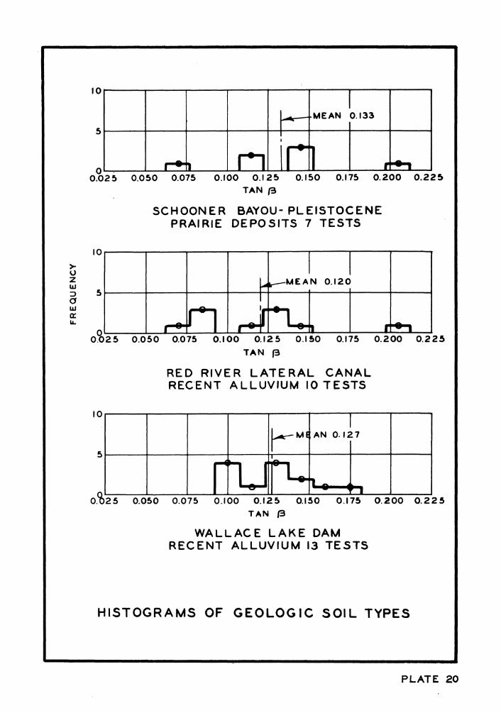
10

.MEAN 0.133

n i

0 .025 0.050 0.075 0.100 0.125 0.150 0.175 0 . 2 0 0 0 . 2 2 5 TAN (B

SCHOONER BAYOU-PLEISTOCENE PRAIRIE DEPOSITS 7 TESTS

10

>• o z UJ

D 5 UJ A

- M E A N 0.120

JtU 0 . 0 2 5 0 .050 0.075 0.100 0.125 0.150 0.175 0 . 2 0 0 0 . 2 2 5

T A N f3

RED RIVER LATERAL CANAL RECENT ALLUVIUM 10 TESTS

10

L*~ M£ AN 0. 12 >7

' .1 fu W-H ^

A 0 . 0 2 5 0.050 0.075 0.100 0.125 0.150 0.175 0 . 2 0 0 0 . 2 2 5 T A N (3

WALLACE LAKE DAM RECENT ALLUVIUM 13 TESTS


PLATE 20

0.050 0.075 0.100 0.125 0.150 0.175 0.200 0.225 0.250 TAN £

MISSISSIPPI BASIN MODEL-TERTIARY (EOCENE) 41 TESTS

10 >-u z UJ D a Id CC

— MEAN f

0.129

^s* • n J ° u_ 'U,

0.050 0.075 0.100 0.125 0.150 0.175 0.200 0.225 0.250 TAN £

GRENADA DAM-RECENT ALLUVIUM 25 TESTS

10 I— MEAr J 0.133 I— MEAr J 0.133

0.050 0.075 0.100 0.125 0.150 0.175 0 .200 0.225 0 .250 TAN P

GRENADA DAM-TERTIARY (EOCENE) 69 TESTS


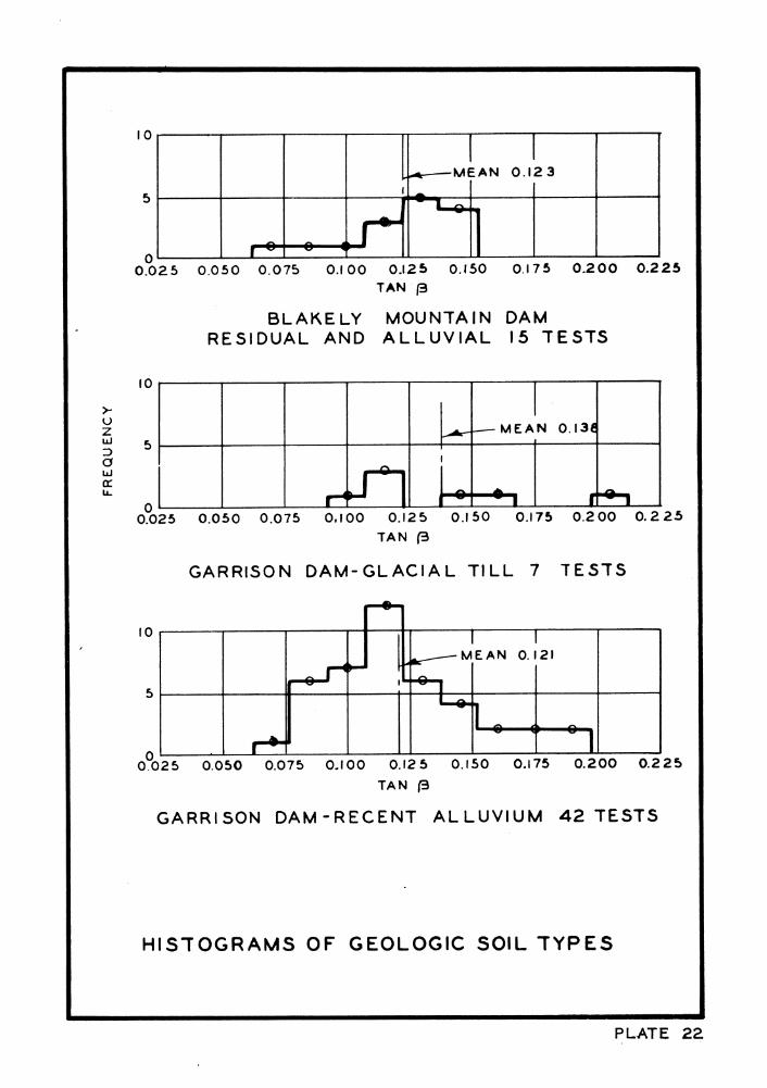
10

r s -MEAN 0.123

i 0.025 0.050 0.075 0.100 0.125 0.150 0.175 0.200 0.225

TAN (3

BLAKELY MOUNTAIN DAM RESIDUAL AND A L L U V I A L 15 TESTS

10

>-o z UJ D a UJ

cr u.

MEAN 0.136

r* -n 1

-^i f^i 0.025 0.050 0.075 0,100 0.125 0.150 0.175 0.2 00 0 . 2 2 5

TAN (3

GARRISON D A M - G L A C I A L T ILL 7 TESTS

MEAN 0.121

^ i & (> o

0.025 0.050 0.075 0.100 0.125 0.150 0.175 0.200 0.225 TAN (3

GARRISON D A M - R E C E N T A L L U V I U M 4 2 TESTS


PLATE 22

mississippi river commission

Documents