mining survey data for swot analysis - eprints · mining survey data for swot analysis by boonyarat...
TRANSCRIPT

UNIVERSITY OF SOUTHAMPTON
FACULTY OF PHYSICAL SCIENCES AND ENGINEERING
Electronics and Computer Science
Mining Survey Data for SWOT Analysis
by
Boonyarat Phadermrod
A thesis submitted for the degree of Doctor of Philosophy
November 4, 2016

UNIVERSITY OF SOUTHAMPTON
ABSTRACT
FACULTY OF PHYSICAL SCIENCES AND ENGINEERINGElectronics and Computer Science
Doctor of Philosophy
MINING SURVEY DATA FOR SWOT ANALYSIS
by Boonyarat Phadermrod
Strengths, Weaknesses, Opportunities and Threats (SWOT) analysis is one of the mostimportant tools for strategic planning. The traditional method of conducting SWOTanalysis does not prioritize and is likely to hold subjective views that may result in animproper strategic action. Accordingly, this research exploits Importance-PerformanceAnalysis (IPA), a technique for measuring customers’ satisfaction based on survey data,to systematically generate prioritized SWOT factors based on customers’ perspectiveswhich in turn produces more accurate information for strategic planning. This proposedapproach is called IPA based SWOT analysis and its development issues discussed inthis report are: (1) selecting a technique for measuring importance which is one ofthe two main aspects of IPA since currently there are no well-established approaches formeasuring importance; and (2) identifying opportunities and threats since only strengthsand weaknesses can be inferred from the IPA result.
The first issue is addressed by conducting an empirical comparison to analyse the perfor-mance of various techniques for measuring importance. Specifically, this thesis considerstwo data mining techniques namely Naïve Bayes and Bayesian Networks for measuringimportance and compares their performance with other techniques namely MultipleLinear Regressions, Ordinal Logistic Regression and Back Propagation Neural Networksthat have been used to derive the importance from the survey data. The comparison re-sult measured against the evaluation metrics suggests that Multiple Linear Regressionsis the most suitable technique for measuring importance.
Regarding the second issue, opportunities and threats were identified by comparing theIPA result of the target organisation with that of its competitor. Through the use ofIPA based SWOT analysis, it is expected that an organisation can efficiently formulatestrategic planning as the SWOT factors that should be maintained or improved canbe clearly identified based on customers’ viewpoints. The application of the IPA basedSWOT analysis was illustrated and evaluated through a case study of Higher EducationInstitutions in Thailand. The evaluation results showed that SWOT analysis of the case

ii
study has a high face validity and its quality is considered acceptable, thereby demon-strating the validity of this study. Although the application of IPA based SWOT analysiswas illustrated in the specific field, it can be argued that IPA based SWOT analysis canbe used widely in the other business areas where SWOT analysis has been seen to beapplicable and the customer satisfaction surveys are generally conducted.

Contents
Declaration of Authorship xxi
Acknowledgements xxiii
Abbreviations Used xxv
1 Introduction 11.1 Research challenges . . . . . . . . . . . . . . . . . . . . . . . . . . . . . . . 31.2 Research questions . . . . . . . . . . . . . . . . . . . . . . . . . . . . . . . 31.3 Outline of the thesis . . . . . . . . . . . . . . . . . . . . . . . . . . . . . . 41.4 Publication list . . . . . . . . . . . . . . . . . . . . . . . . . . . . . . . . . 6
2 Literature Review 72.1 SWOT analysis . . . . . . . . . . . . . . . . . . . . . . . . . . . . . . . . . 7
2.1.1 SWOT analysis matrix . . . . . . . . . . . . . . . . . . . . . . . . . 82.1.2 Advantages and Disadvantages of SWOT analysis . . . . . . . . . 82.1.3 Quantitative SWOT analysis . . . . . . . . . . . . . . . . . . . . . 92.1.4 Research in SWOT analysis system . . . . . . . . . . . . . . . . . . 10
2.2 Data Mining . . . . . . . . . . . . . . . . . . . . . . . . . . . . . . . . . . 112.2.1 Data mining methods . . . . . . . . . . . . . . . . . . . . . . . . . 122.2.2 Classification and Prediction Techniques . . . . . . . . . . . . . . . 14
2.2.2.1 Multiple Linear Regressions . . . . . . . . . . . . . . . . . 142.2.2.2 Ordinal Logistic Regressions . . . . . . . . . . . . . . . . 152.2.2.3 Back Propagation Neural Networks . . . . . . . . . . . . 182.2.2.4 Naïve Bayes . . . . . . . . . . . . . . . . . . . . . . . . . 202.2.2.5 Bayesian Networks . . . . . . . . . . . . . . . . . . . . . . 22
2.3 Customer Satisfaction . . . . . . . . . . . . . . . . . . . . . . . . . . . . . 242.3.1 Overview of customer satisfaction . . . . . . . . . . . . . . . . . . . 242.3.2 Measuring customer satisfaction . . . . . . . . . . . . . . . . . . . 252.3.3 Analysis of Customer satisfaction data . . . . . . . . . . . . . . . . 27
2.3.3.1 Descriptive statistics . . . . . . . . . . . . . . . . . . . . . 272.3.3.2 Statistical and modern approaches . . . . . . . . . . . . . 27
2.3.4 Research on mining customer satisfaction data . . . . . . . . . . . 282.4 Summary . . . . . . . . . . . . . . . . . . . . . . . . . . . . . . . . . . . . 32
3 Importance-Performance Analysis 353.1 Overview of Importance-Performance Analysis . . . . . . . . . . . . . . . 35
3.1.1 IPA matrix . . . . . . . . . . . . . . . . . . . . . . . . . . . . . . . 36
iii

iv CONTENTS
3.1.2 Developing the IPA matrix . . . . . . . . . . . . . . . . . . . . . . 383.1.3 Approaches for measuring performance . . . . . . . . . . . . . . . . 403.1.4 Approaches for measuring importance . . . . . . . . . . . . . . . . 40
3.2 Previous comparative studies of methods for measuring importance . . . . 453.3 Methodology for deriving importance . . . . . . . . . . . . . . . . . . . . . 49
3.3.1 Method for deriving importance based on MLR . . . . . . . . . . . 493.3.2 Method for deriving importance based on OLR . . . . . . . . . . . 503.3.3 Method for deriving importance based on BPNN . . . . . . . . . . 503.3.4 Method for deriving importance based on Naïve Bayes . . . . . . . 523.3.5 Method for deriving importance based on BNs . . . . . . . . . . . 54
3.4 Summary . . . . . . . . . . . . . . . . . . . . . . . . . . . . . . . . . . . . 55
4 Research Design 574.1 An overview of research design within this study . . . . . . . . . . . . . . 574.2 Problem identification . . . . . . . . . . . . . . . . . . . . . . . . . . . . . 624.3 Solution design: IPA . . . . . . . . . . . . . . . . . . . . . . . . . . . . . . 634.4 Solution design: IPA-SWOT . . . . . . . . . . . . . . . . . . . . . . . . . . 644.5 Evaluation through the survey research . . . . . . . . . . . . . . . . . . . 65
4.5.1 Selecting survey media . . . . . . . . . . . . . . . . . . . . . . . . . 664.5.2 Selecting survey questions . . . . . . . . . . . . . . . . . . . . . . . 664.5.3 Selecting contact method . . . . . . . . . . . . . . . . . . . . . . . 674.5.4 Selecting administration method . . . . . . . . . . . . . . . . . . . 67
4.6 Summary . . . . . . . . . . . . . . . . . . . . . . . . . . . . . . . . . . . . 68
5 Experiment: Empirical comparison of importance measuring tech-niques 715.1 Preliminary study . . . . . . . . . . . . . . . . . . . . . . . . . . . . . . . 72
5.1.1 Replication of the IPA based MI . . . . . . . . . . . . . . . . . . . 725.1.2 Comparative Analysis of Classification Algorithms using WEKA . 73
5.2 Evaluation Metrics . . . . . . . . . . . . . . . . . . . . . . . . . . . . . . . 735.2.1 Predictive validity . . . . . . . . . . . . . . . . . . . . . . . . . . . 735.2.2 Diagnosticity . . . . . . . . . . . . . . . . . . . . . . . . . . . . . . 745.2.3 Discriminating power . . . . . . . . . . . . . . . . . . . . . . . . . 75
5.3 Datasets . . . . . . . . . . . . . . . . . . . . . . . . . . . . . . . . . . . . . 765.3.1 Dataset A . . . . . . . . . . . . . . . . . . . . . . . . . . . . . . . . 765.3.2 Dataset B . . . . . . . . . . . . . . . . . . . . . . . . . . . . . . . . 775.3.3 Dataset C . . . . . . . . . . . . . . . . . . . . . . . . . . . . . . . . 77
5.4 Methodology . . . . . . . . . . . . . . . . . . . . . . . . . . . . . . . . . . 775.4.1 Data pre-processing . . . . . . . . . . . . . . . . . . . . . . . . . . 785.4.2 Model Training . . . . . . . . . . . . . . . . . . . . . . . . . . . . . 79
5.4.2.1 Parameter setting . . . . . . . . . . . . . . . . . . . . . . 805.4.2.2 Model quality . . . . . . . . . . . . . . . . . . . . . . . . 84
5.4.3 Obtaining importance . . . . . . . . . . . . . . . . . . . . . . . . . 865.5 Summary . . . . . . . . . . . . . . . . . . . . . . . . . . . . . . . . . . . . 90
6 Results and Discussion: Empirical comparison of importance measur-ing 936.1 The test of convergent validity of different importance measure . . . . . . 93

CONTENTS v
6.1.1 Results of convergent validity for each dataset . . . . . . . . . . . . 936.1.2 Convergent Validity Findings . . . . . . . . . . . . . . . . . . . . . 96
6.2 Result of the empirical comparison . . . . . . . . . . . . . . . . . . . . . . 976.2.1 Predictive validity . . . . . . . . . . . . . . . . . . . . . . . . . . . 976.2.2 Diagnosticity . . . . . . . . . . . . . . . . . . . . . . . . . . . . . . 986.2.3 Discriminating power . . . . . . . . . . . . . . . . . . . . . . . . . 996.2.4 Summary of comparative results . . . . . . . . . . . . . . . . . . . 100
6.3 Statistical analysis of the results for the empirical comparison . . . . . . . 1016.3.1 Statistical test of Predictive validity . . . . . . . . . . . . . . . . . 1016.3.2 Statistical test of Diagnosticity . . . . . . . . . . . . . . . . . . . . 1056.3.3 Statistical test of Discriminating power . . . . . . . . . . . . . . . 107
6.4 Discussion of the results for the empirical comparison . . . . . . . . . . . 1106.5 Summary . . . . . . . . . . . . . . . . . . . . . . . . . . . . . . . . . . . . 115
7 IPA based SWOT analysis 1177.1 Background of IPA based SWOT analysis . . . . . . . . . . . . . . . . . . 1177.2 IPA based SWOT analysis Framework . . . . . . . . . . . . . . . . . . . . 1197.3 Summary . . . . . . . . . . . . . . . . . . . . . . . . . . . . . . . . . . . . 123
8 IPA based SWOT analysis: Evaluation Methodology 1258.1 Background of the case study . . . . . . . . . . . . . . . . . . . . . . . . . 1268.2 Methodology for conducting student satisfaction survey . . . . . . . . . . 127
8.2.1 Questionnaire design . . . . . . . . . . . . . . . . . . . . . . . . . . 1278.2.2 Consistency of the translation between English and Thai version
of questionnaire . . . . . . . . . . . . . . . . . . . . . . . . . . . . . 1288.2.3 Sample size estimation . . . . . . . . . . . . . . . . . . . . . . . . . 1288.2.4 Ethics . . . . . . . . . . . . . . . . . . . . . . . . . . . . . . . . . . 1298.2.5 Pilot study . . . . . . . . . . . . . . . . . . . . . . . . . . . . . . . 1298.2.6 Data collection . . . . . . . . . . . . . . . . . . . . . . . . . . . . . 1308.2.7 Data analysis method . . . . . . . . . . . . . . . . . . . . . . . . . 132
8.3 Implementation of IPA based SWOT analysis . . . . . . . . . . . . . . . . 1328.4 Methodology for conducting staff evaluation of SWOT survey . . . . . . . 134
8.4.1 Questionnaire design . . . . . . . . . . . . . . . . . . . . . . . . . . 1348.4.2 Consistency of the translation between English and Thai version
of questionnaire . . . . . . . . . . . . . . . . . . . . . . . . . . . . . 1358.4.3 Sample size estimation . . . . . . . . . . . . . . . . . . . . . . . . . 1358.4.4 Ethics . . . . . . . . . . . . . . . . . . . . . . . . . . . . . . . . . . 1368.4.5 Pilot study . . . . . . . . . . . . . . . . . . . . . . . . . . . . . . . 1368.4.6 Data collection . . . . . . . . . . . . . . . . . . . . . . . . . . . . . 1388.4.7 Data analysis method . . . . . . . . . . . . . . . . . . . . . . . . . 138
8.5 Methodology for conducting experienced users of SWOT survey . . . . . . 1398.5.1 Questionnaire design . . . . . . . . . . . . . . . . . . . . . . . . . . 1408.5.2 Consistency of the translation between English and Thai version
of questionnaire . . . . . . . . . . . . . . . . . . . . . . . . . . . . . 1418.5.3 Sample size estimation . . . . . . . . . . . . . . . . . . . . . . . . . 1428.5.4 Ethics . . . . . . . . . . . . . . . . . . . . . . . . . . . . . . . . . . 1438.5.5 Pilot study . . . . . . . . . . . . . . . . . . . . . . . . . . . . . . . 143
vi CONTENTS
8.5.6 Data collection . . . . . . . . . . . . . . . . . . . . . . . . . . . . . 1438.5.7 Data analysis method . . . . . . . . . . . . . . . . . . . . . . . . . 145
8.6 Summary . . . . . . . . . . . . . . . . . . . . . . . . . . . . . . . . . . . . 146
9 IPA based SWOT analysis: Evaluation Results 1499.1 Results of IPA based SWOT analysis of the case study . . . . . . . . . . . 149
9.1.1 IPA matrix of the two departments . . . . . . . . . . . . . . . . . . 1499.1.2 SWOT matrix of CPE-KU-KPS . . . . . . . . . . . . . . . . . . . 151
9.2 Results of staff evaluation on the SWOT of the case study . . . . . . . . . 1559.2.1 Analytical results of staff evaluation on individual SWOT factor . 1569.2.2 Analytical results of staff evaluation on the group of SWOT factor 158
9.3 Results of SWOT experienced users evaluation on the SWOT of the casestudy . . . . . . . . . . . . . . . . . . . . . . . . . . . . . . . . . . . . . . . 161
9.4 Summary . . . . . . . . . . . . . . . . . . . . . . . . . . . . . . . . . . . . 163
10 Discussion 16510.1 Discussion of Empirical comparison . . . . . . . . . . . . . . . . . . . . . 16510.2 Discussion of IPA based SWOT analysis and its application . . . . . . . . 16810.3 Discussion of evaluation result of IPA based SWOT analysis . . . . . . . . 170
10.3.1 Discussion of staff evaluation on the SWOT of the case study . . . 17010.3.2 Discussion of SWOT experienced users evaluation on the SWOT
of the case study . . . . . . . . . . . . . . . . . . . . . . . . . . . . 17110.3.3 Discussion of sample size for the SWOT evaluation surveys . . . . 172
10.4 Limitations of the present study . . . . . . . . . . . . . . . . . . . . . . . 17210.4.1 Limitations of the empirical study . . . . . . . . . . . . . . . . . . 17310.4.2 Limitations of the proposed framework . . . . . . . . . . . . . . . . 17310.4.3 Limitation of evaluation of IPA based SWOT analysis . . . . . . . 174
11 Conclusion and Future work 17511.1 Contributions . . . . . . . . . . . . . . . . . . . . . . . . . . . . . . . . . . 17711.2 Future work . . . . . . . . . . . . . . . . . . . . . . . . . . . . . . . . . . . 178
11.2.1 Investigating another technical issue of IPA . . . . . . . . . . . . . 17811.2.2 Exploring the other evaluation metrics or justifying the weight of
evaluation metrics . . . . . . . . . . . . . . . . . . . . . . . . . . . 17911.2.3 Considering the other data mining techniques or a combination of
techniques in measuring importance . . . . . . . . . . . . . . . . . 17911.2.4 Developing a prototype system of IPA based SWOT analysis . . . 17911.2.5 Investigating a method to identify macro external factor . . . . . 181
11.3 Summary of Thesis . . . . . . . . . . . . . . . . . . . . . . . . . . . . . . . 181
Appendix A Replication of the IPA based Mutual Information 183A.1 Tools . . . . . . . . . . . . . . . . . . . . . . . . . . . . . . . . . . . . . . . 183A.2 Methodology . . . . . . . . . . . . . . . . . . . . . . . . . . . . . . . . . . 183A.3 IPA based MI results . . . . . . . . . . . . . . . . . . . . . . . . . . . . . . 186A.4 Statistical test of IPA based MI results . . . . . . . . . . . . . . . . . . . . 188
Appendix B Comparative Analysis of Classification Algorithms usingWEKA 193

CONTENTS vii
B.1 Dataset and Tool . . . . . . . . . . . . . . . . . . . . . . . . . . . . . . . . 193B.2 Methodology . . . . . . . . . . . . . . . . . . . . . . . . . . . . . . . . . . 194B.3 Result . . . . . . . . . . . . . . . . . . . . . . . . . . . . . . . . . . . . . . 195
Appendix C Assumption checking of the multiple linear regressions on 3datasets 197C.1 Assumption checking of the multiple linear regressions on dataset A . . . 198C.2 Assumption checking of the multiple linear regressions on dataset B . . . 204C.3 Assumption checking of the multiple linear regressions on dataset C . . . 211
Appendix D Assumption checking of the ordinal logistic regressions on 3datasets 223
Appendix E Assigning number of hidden-layer neurons 225E.1 Regression model of BPNN . . . . . . . . . . . . . . . . . . . . . . . . . . 226E.2 Classification model of BPNN . . . . . . . . . . . . . . . . . . . . . . . . . 227
Appendix F Computational example of importance measures 231F.1 Computational example for computing importance from Multiple Linear
Regression . . . . . . . . . . . . . . . . . . . . . . . . . . . . . . . . . . . . 231F.2 Computational example for computing importance from Ordinal Linear
Regression . . . . . . . . . . . . . . . . . . . . . . . . . . . . . . . . . . . . 233F.3 Computational example for computing importance from neural network . 233F.4 Computational example for computing importance from Naïve Bayes . . . 236F.5 Computational example for computing importance from Bayesian Networks239
F.5.1 Pre-calculation procedure . . . . . . . . . . . . . . . . . . . . . . . 240F.5.2 Calculate importance as Mutual Information . . . . . . . . . . . . 244
Appendix G Student satisfaction survey material 247G.1 Student Satisfaction Survey . . . . . . . . . . . . . . . . . . . . . . . . . . 247G.2 Participant Information sheet . . . . . . . . . . . . . . . . . . . . . . . . . 250G.3 Result of language consistency translation test of student satisfaction survey251
Appendix H Assumption checking of the multiple linear regressionon CPE-KU-KPS dataset 257H.1 Normally distributed residual . . . . . . . . . . . . . . . . . . . . . . . . . 258H.2 Linear relationship between independent and dependent variables . . . . . 260H.3 Homoscedasticity of residuals . . . . . . . . . . . . . . . . . . . . . . . . . 268H.4 Independence of residual . . . . . . . . . . . . . . . . . . . . . . . . . . . . 269H.5 Multicollinearity . . . . . . . . . . . . . . . . . . . . . . . . . . . . . . . . 269
Appendix I Assumption checking of the multiple linear regressionon CPE-KU-BKN dataset 273I.1 Normally distributed residual . . . . . . . . . . . . . . . . . . . . . . . . . 274I.2 Linear relationship between independent and dependent variables . . . . . 276I.3 Homoscedasticity of residuals . . . . . . . . . . . . . . . . . . . . . . . . . 285I.4 Independence of residual . . . . . . . . . . . . . . . . . . . . . . . . . . . . 285I.5 Multicollinearity . . . . . . . . . . . . . . . . . . . . . . . . . . . . . . . . 286

viii CONTENTS
Appendix J Staff evaluation of SWOT survey material 289J.1 Survey on the level of agreement toward SWOT of department . . . . . . 289J.2 Participant Information sheet . . . . . . . . . . . . . . . . . . . . . . . . . 293J.3 Result of language consistency translation test of staff evaluation of SWOT
survey . . . . . . . . . . . . . . . . . . . . . . . . . . . . . . . . . . . . . . 294
Appendix K Assumption checking of one sample t-test for staff evaluationon SWOT factor 301K.1 Result of the assumptions test of one sample t-test on staff agreement
level of SWOT factor . . . . . . . . . . . . . . . . . . . . . . . . . . . . . . 301K.2 Result of the normality test for one sample t-test on the transformed staff
agreement level of SWOT factor . . . . . . . . . . . . . . . . . . . . . . . 307
Appendix L Assumption checking of one sample t-test for staff evaluationon the group of SWOT factor 315
Appendix M Experienced users of SWOT survey material 319M.1 Questionnaire on the quality of an outcome of IPA based SWOT . . . . . 319M.2 Questionnaire on the quality of an outcome of Traditional SWOT . . . . . 325M.3 Participant Information sheet . . . . . . . . . . . . . . . . . . . . . . . . . 328M.4 Result of language consistency translation test of experienced users of
SWOT survey . . . . . . . . . . . . . . . . . . . . . . . . . . . . . . . . . . 329
Appendix N Assumption checking of two independent sample t-teston experienced users of SWOT evaluation 337
References 341

List of Figures
1.1 IPA matrix represented major/minor strengths and weaknesses adaptedfrom Garver (2003) . . . . . . . . . . . . . . . . . . . . . . . . . . . . . . . 2
1.2 Diagram shows the relationship between the thesis chapters and the re-search questions . . . . . . . . . . . . . . . . . . . . . . . . . . . . . . . . . 5
2.1 The SWOT analysis matrix . . . . . . . . . . . . . . . . . . . . . . . . . . 82.2 A 3-3-2 structure of a multilayer feed-forward network . . . . . . . . . . . 182.3 Back propagation of Errors for a Single Neuron (Turban et al., 2008) . . . 192.4 The structure of a Naïve Bayes network (Friedman et al., 1997) . . . . . . 202.5 The backache BN example adapted from (Ben-Gal, 2007). Each node
represents variable with its conditional probability table. . . . . . . . . . . 22
3.1 The IPA matrix (Hosseini and Bideh, 2013) . . . . . . . . . . . . . . . . . 373.2 Steps for constructing IPA matrix . . . . . . . . . . . . . . . . . . . . . . 38
4.1 Research design scenario . . . . . . . . . . . . . . . . . . . . . . . . . . . . 60
5.1 The overall procedure of the empirical comparison. . . . . . . . . . . . . . 785.2 The 6-2-1 neural network as applied to dataset A. . . . . . . . . . . . . . 825.3 The 6-6-6 neural network as applied to dataset A. . . . . . . . . . . . . . 825.4 The structure of Naïve Bayes network as applied to dataset A. . . . . . . 835.5 The structure of Bayesian network as applied to dataset A . . . . . . . . . 835.6 Percentage accuracy of different models across three datasets . . . . . . . 875.7 RMSE of different models across three datasets . . . . . . . . . . . . . . . 87
7.1 IPA matrix as SWOT (Kim and Oh, 2001) . . . . . . . . . . . . . . . . . 1187.2 Proposed framework for applying IPA to SWOT analysis . . . . . . . . . 1197.3 Steps for conducting IPA of customer survey data . . . . . . . . . . . . . . 120
9.1 IPA matrix of CPE-KU-KPS. Each point represents a pair of importanceand performance for each factor presented in the second and third columnof Table 9.1. The IPA matrix is separated into four quadrants regardingto the intersection of the Grand Mean of importance and performancewhich represented as red horizontal line and red vertical line. . . . . . . . 152
9.2 IPA matrix of CPE-KU-BKN. Each point represents a pair of importanceand performance for each factor presented in the fifth and sixth column ofTable 9.1. The IPA matrix is separated into four quadrants regarding tothe intersection of the Grand Mean of importance and performance whichrepresented as red horizontal line and red vertical line. . . . . . . . . . . 153
ix

x LIST OF FIGURES
9.3 Simple error bar of the four variables of each SWOT group. The mean isrepresented by a dot, a line represents standard error of the mean, a redhorizontal line is represented the threshold score of 2.5. . . . . . . . . . . 158
9.4 Simple error bar of the three variables of SWOT group. The mean isrepresented by a dot, a line represents standard error of the mean, a redhorizontal line is represented the threshold score of 3.0 . . . . . . . . . . . 160
11.1 The proposed system architecture of IPA based SWOT analysis . . . . . . 180
A.1 IPA based MI matrix from experiment. . . . . . . . . . . . . . . . . . . . . 186A.2 IPA based MI matrix from referenced paper (Cugnata and Salini, 2013) . 187A.3 The normal quantile plot of importance from different sources . . . . . . . 189
C.1 Histogram and normality plots of residual (dataset A) . . . . . . . . . . . 198C.2 Scatterplot of residual for the relationship between six independent vari-
ables and the Satisfaction (dataset A) . . . . . . . . . . . . . . . . . . . . 199C.3 Partial regression plots of each independent variable against Satisfaction
(dataset A) . . . . . . . . . . . . . . . . . . . . . . . . . . . . . . . . . . . 200C.4 Scatterplot with model curve fit of each independent variable against
Satisfaction (dataset A) . . . . . . . . . . . . . . . . . . . . . . . . . . . . 202C.5 Histogram and normality plots of residual (dataset B) . . . . . . . . . . . 205C.6 Scatterplot of residual for the relationship between 13 independent vari-
ables and the V56 (dataset B) . . . . . . . . . . . . . . . . . . . . . . . . . 205C.7 Partial regression plots of independent variable V42-V47 against V56
(dataset B) . . . . . . . . . . . . . . . . . . . . . . . . . . . . . . . . . . . 206C.8 Partial regression plots of independent variable V48-V54 against V56
(dataset B) . . . . . . . . . . . . . . . . . . . . . . . . . . . . . . . . . . . 216C.9 Scatterplot with model curve fit of independent variable V42-V49 against
V56 (dataset B) . . . . . . . . . . . . . . . . . . . . . . . . . . . . . . . . . 217C.10 Scatterplot with model curve fit of independent variable V50-V54 against
V56 (dataset B) . . . . . . . . . . . . . . . . . . . . . . . . . . . . . . . . . 218C.11 Histogram and normality plots of residual (dataset C) . . . . . . . . . . . 219C.12 Scatterplot of residual for the relationship between six independent vari-
ables and the OCS student (dataset C) . . . . . . . . . . . . . . . . . . . . 219C.13 Partial regression plots of each independent variable against OCS student
(dataset C) . . . . . . . . . . . . . . . . . . . . . . . . . . . . . . . . . . . 220C.14 Scatterplot with model curve fit of each independent variable against OCS
student (dataset C) . . . . . . . . . . . . . . . . . . . . . . . . . . . . . . . 221
F.1 Result of multiple linear regression implemented on dataset A . . . . . . 232F.2 Result of ordinal linear regression implemented on dataset A . . . . . . . 234F.3 The conditional probability distribution of attribute ContractandPrice . . 240F.4 The conditional probability distribution of attribute Equipment . . . . . . 241
H.1 Histogram and normality plots of residual (Teacher) . . . . . . . . . . . . 258H.2 Histogram and normality plots of residual (Teaching) . . . . . . . . . . . . 258H.3 Histogram and normality plots of residual (Admin) . . . . . . . . . . . . . 259H.4 Histogram and normality plots of residual (CompFac) . . . . . . . . . . . 259H.5 Histogram and normality plots of residual (xActivity) . . . . . . . . . . . 260

LIST OF FIGURES xi
H.6 Histogram and normality plots of residual (AddService) . . . . . . . . . . 260H.7 Scatterplot of residual for the relationship between five independent vari-
ables of attribute Teacher and the OCS student . . . . . . . . . . . . . . . 261H.8 Scatterplot of residual for the relationship between six independent vari-
ables of attribute Teaching and the OCS student . . . . . . . . . . . . . . 262H.9 Scatterplot of residual for the relationship between five independent vari-
ables of attribute Admin and the OCS student . . . . . . . . . . . . . . . 263H.10 Scatterplot of residual for the relationship between four independent vari-
ables of attribute CompFac and the OCS student . . . . . . . . . . . . . . 264H.11 Scatterplot of residual for the relationship between seven independent
variables of attribute xActivity and the OCS student . . . . . . . . . . . . 265H.12 Scatterplot of residual for the relationship between four independent vari-
ables of attribute AddService and the OCS student . . . . . . . . . . . . . 266
I.1 Histogram and normality plots of residual (Teacher) . . . . . . . . . . . . 275I.2 Histogram and normality plots of residual (Teaching) . . . . . . . . . . . . 275I.3 Histogram and normality plots of residual (Admin) . . . . . . . . . . . . . 276I.4 Histogram and normality plots of residual (CompFac) . . . . . . . . . . . 276I.5 Histogram and normality plots of residual (xActivity) . . . . . . . . . . . 277I.6 Histogram and normality plots of residual (AddService) . . . . . . . . . . 277I.7 Scatterplot of residual for the relationship between five independent vari-
ables of attribute Teacher and the OCS student . . . . . . . . . . . . . . . 278I.8 Scatterplot of residual for the relationship between six independent vari-
ables of attribute Teaching and the OCS student . . . . . . . . . . . . . . 278I.9 Scatterplot of residual for the relationship between five independent vari-
ables of attribute Admin and the OCS student . . . . . . . . . . . . . . . 279I.10 Scatterplot of residual for the relationship between four independent vari-
ables of attribute CompFac and the OCS student . . . . . . . . . . . . . . 279I.11 Scatterplot of residual for the relationship between seven independent
variables of attribute xActivity and the OCS student . . . . . . . . . . . . 280I.12 Scatterplot of residual for the relationship between four independent vari-
ables of attribute AddService and the OCS student . . . . . . . . . . . . . 280
K.1 Box plots of variables SW1−15 . . . . . . . . . . . . . . . . . . . . . . . . 304K.2 Box plots of variables OT1−16 . . . . . . . . . . . . . . . . . . . . . . . . . 305
L.1 Box plots of variables Savg, Wavg, Oavg and Tavg . . . . . . . . . . . . . . 317
M.1 Steps for generating SWOT based on customers satisfaction survey . . . . 320M.2 Steps for generating SWOT through brainstorming . . . . . . . . . . . . . 328


List of Tables
2.1 Data mining methods and their applications . . . . . . . . . . . . . . . . . 132.2 Publications that applied data mining techniques in analysis of customer
satisfaction data . . . . . . . . . . . . . . . . . . . . . . . . . . . . . . . . 29
3.1 Publications that implicitly derived importance . . . . . . . . . . . . . . . 443.2 Summary of previous comparative studies . . . . . . . . . . . . . . . . . . 483.3 Evaluation metrics and their number of times used in the past compara-
tive studies . . . . . . . . . . . . . . . . . . . . . . . . . . . . . . . . . . . 49
4.1 A summary of design science research activities presented in Peffers et al.(2007) . . . . . . . . . . . . . . . . . . . . . . . . . . . . . . . . . . . . . . 59
4.2 MIS Methodologies retained for this research based on Palvia et al. (2004) 604.3 Connection between the design science research process, research meth-
ods, research questions, and thesis chapters . . . . . . . . . . . . . . . . . 624.4 Detail of three surveys used for demonstration and evaluation of IPA
based SWOT analysis . . . . . . . . . . . . . . . . . . . . . . . . . . . . . 654.5 Comparison of the main aspects of three self-administered method . . . . 69
5.1 Basic characteristics of the datasets . . . . . . . . . . . . . . . . . . . . . . 765.2 Number of records across datasets . . . . . . . . . . . . . . . . . . . . . . 795.3 List of model for measuring importance in this experiment . . . . . . . . . 805.4 Parameter setting of two BPNN structure models . . . . . . . . . . . . . . 815.5 Number of hidden-layer neurons and network structure for each BPNN
model of three datasets . . . . . . . . . . . . . . . . . . . . . . . . . . . . 815.6 Accuracy and RMSE of models using different techniques on dataset A . . 855.7 Accuracy and RMSE of models using different techniques on dataset B . . 855.8 Accuracy and RMSE of models using different techniques on dataset C . . 865.9 Importance measured by using different techniques on dataset A (per-
centage). Values in bold are the highest importance measure while valuesunderlined are the lowest importance measure. . . . . . . . . . . . . . . . 88
5.10 Importance measured by using different techniques on dataset B (per-centage). Values in bold are the highest importance measure while valuesunderlined are the lowest importance measure. . . . . . . . . . . . . . . . 89
5.11 Importance measured by using different techniques on dataset C (per-centage). Values in bold are the highest importance measure while valuesunderlined are the lowest importance measure. . . . . . . . . . . . . . . . 90
6.1 Convergence validity of importance measuring techniques (Dataset A) . . 946.2 Convergence validity of importance measuring techniques (Dataset B) . . 94
xiii

xiv LIST OF TABLES
6.3 Convergence validity of importance measuring techniques (Dataset C) . . 956.4 A measure of predictive validity as correlation coefficient between multi-
attribute attitude model predictions with overall satisfaction. The highercorrelation coefficient (close to 1) indicates the better predictive validity. . 97
6.5 A measure of diagnosticity as non-linear regression coefficient (β2) of therelationship between importance and rank. The lower the value of non-linear regression coefficient indicates the better diagnosticity. . . . . . . . 98
6.6 A measure of discriminating power as F-statistic between attribute dis-crimination. The larger F-statistic indicates the better discriminatingpower. . . . . . . . . . . . . . . . . . . . . . . . . . . . . . . . . . . . . . . 99
6.7 The ranking of techniques according to the tree evaluation metrics (Thelower the rank, the better theimportance measure) . . . . . . . . . . . . . 102
6.8 Significance tests for differences in predictive ability (Dataset A) . . . . . 1036.9 Significance tests for differences in predictive ability (Dataset B) . . . . . 1046.10 Significance tests for differences in predictive ability (Dataset C) . . . . . 1046.11 Significance tests for differences in diagnosticity (Dataset A) . . . . . . . . 1056.12 Significance tests for differences in diagnosticity (Dataset B) . . . . . . . . 1066.13 Significance tests for differences in diagnosticity (Dataset C) . . . . . . . . 1066.14 partial eta squared and correlation coefficient corresponded to F-statistics
of each technique . . . . . . . . . . . . . . . . . . . . . . . . . . . . . . . . 1076.15 Chi-square statistic for the difference test of several independent correlations1086.16 Significance tests for differences in correlations obtained from F-statistics
(Dataset A) . . . . . . . . . . . . . . . . . . . . . . . . . . . . . . . . . . . 1096.17 Significance tests for differences in correlations obtained from F-statistics
(Dataset B) . . . . . . . . . . . . . . . . . . . . . . . . . . . . . . . . . . . 1096.18 Significance tests for differences in correlations obtained from F-statistics
(Dataset C) . . . . . . . . . . . . . . . . . . . . . . . . . . . . . . . . . . . 110
7.1 SWOT identification table . . . . . . . . . . . . . . . . . . . . . . . . . . . 122
8.1 Minimum required sample size for building multiple linear regressionmodel of each attribute . . . . . . . . . . . . . . . . . . . . . . . . . . . . 129
8.2 List of attributes used in the case study and Cronbach’s alpha . . . . . . 1308.3 General characteristics of sample CPE-KU-KPS students (N=155) . . . . 1318.4 General characteristics of sample CPE-KU-BKN students (N=43) . . . . 1328.5 Opinion regarding to the design of staff evaluation of SWOT questionnaire1378.6 General characteristics of sample CPE-KU-KPS staff (N=14) . . . . . . . 1388.7 List of questions in the experienced users of SWOT survey . . . . . . . . . 1418.8 Opinion regarding to the design of questionnaire of experienced SWOT
user . . . . . . . . . . . . . . . . . . . . . . . . . . . . . . . . . . . . . . . 1448.9 General characteristics of two groups of MBA students (N=22) . . . . . . 145
9.1 Importance-Performance of the two departments. Each row representsimportance, performance and IPA quadrant of the two departments. Thesecond last row represents the mean of importance and performance foreach department in which their overall mean (Grand Mean) is representedin the last row. . . . . . . . . . . . . . . . . . . . . . . . . . . . . . . . . . 150

LIST OF TABLES xv
9.2 Result of IPA based SWOT. Each row represents the factor which labelledas strength-weakness of the two departments, SWOT of CPE-KU-KPS,and its weight. For each factor, its weight is computed as the product ofimportance and performance of CPE-KU-KPS shown in Table 9.1 . . . . . 154
9.3 SWOT matrix of CPE-KU-KPS . . . . . . . . . . . . . . . . . . . . . . . . 1559.4 Result of one-sample Wilcoxon signed rank test for variable SW1−15 . . . 1569.5 List of strength-weakness variables that their level of staff agreement is
lower than 3.0 . . . . . . . . . . . . . . . . . . . . . . . . . . . . . . . . . 1579.6 Result of one-sample Wilcoxon signed rank test for variable OT1−16 . . . 1579.7 List of opportunity variables that their level of staff agreement is different
from 3.0 . . . . . . . . . . . . . . . . . . . . . . . . . . . . . . . . . . . . . 1579.8 Summary of agreed SWOT factors . . . . . . . . . . . . . . . . . . . . . . 1589.9 Result of the One-sample t-test for each SWOT group (Test value is 2.5) . 1599.10 Result of the One-sample t-test for three SWOT group (Test value is 3.0) 1609.11 The mean and standard deviation of rating score on 10 questions regard-
ing the two SWOT approaches . . . . . . . . . . . . . . . . . . . . . . . . 1619.12 Results of the Mann-Whitney U test (N=22) . . . . . . . . . . . . . . . . 162
10.1 Summary of data sources for the different SWOT analysis approaches andtheir associated analytical techniques . . . . . . . . . . . . . . . . . . . . . 169
A.1 performance and importance of each attribute of company’s service . . . . 186A.2 Comparison of IPA result for this study with that published in referenced
paper . . . . . . . . . . . . . . . . . . . . . . . . . . . . . . . . . . . . . . 187A.3 Estimated performance and importance from Figure A.2 . . . . . . . . . . 188A.4 The importance from difference sources . . . . . . . . . . . . . . . . . . . . 188A.5 The result of correlation coefficient test for normality of the importance . 190A.6 Levene’s Statistic of two groups of importance . . . . . . . . . . . . . . . . 190A.7 T-test: Two-Sample Assuming Equal Variances . . . . . . . . . . . . . . . 191
B.1 Detail of Pima Indians Diabetes Dataset . . . . . . . . . . . . . . . . . . . 194B.2 Detail of Classifiers . . . . . . . . . . . . . . . . . . . . . . . . . . . . . . . 194B.3 Accuracy of different classifiers . . . . . . . . . . . . . . . . . . . . . . . . 195B.4 Different performance metrics in training phase . . . . . . . . . . . . . . . 195B.5 Different performance metrics in testing phase . . . . . . . . . . . . . . . 196
C.1 Summary of assumption checking of MLR on 3 datasets . . . . . . . . . . 197C.2 Descriptive statistic of unstandardized residual (dataset A) . . . . . . . . 198C.3 Model summary corresponded to the scatterplot of Equipment versus Sat-
isfaction . . . . . . . . . . . . . . . . . . . . . . . . . . . . . . . . . . . . . 201C.4 Model summary corresponded to the scatterplot of SaleSup versus Satis-
faction . . . . . . . . . . . . . . . . . . . . . . . . . . . . . . . . . . . . . . 201C.5 Model summary corresponded to the scatterplot of TechSup versus Sat-
isfaction . . . . . . . . . . . . . . . . . . . . . . . . . . . . . . . . . . . . . 201C.6 Model summary corresponded to the scatterplot of Supplier versus Satis-
faction . . . . . . . . . . . . . . . . . . . . . . . . . . . . . . . . . . . . . . 201C.7 Model summary corresponded to the scatterplot of AdminSup versus Sat-
isfaction . . . . . . . . . . . . . . . . . . . . . . . . . . . . . . . . . . . . . 201

xvi LIST OF TABLES
C.8 Model summary corresponded to the scatterplot of TermCond versus Sat-isfaction . . . . . . . . . . . . . . . . . . . . . . . . . . . . . . . . . . . . . 201
C.9 Chi-square statistic for the difference test of several independent correla-tions (dataset A) . . . . . . . . . . . . . . . . . . . . . . . . . . . . . . . . 203
C.10 Collinearity Statistics (VIF) of six independent variables (dataset A) . . . 204C.11 Descriptive statistic of unstandardized residual (dataset B) . . . . . . . . 204C.12 Model summary corresponded to the scatterplot of V42 versus V56 . . . . 207C.13 Model summary corresponded to the scatterplot of V43 versus V56 . . . . 207C.14 Model summary corresponded to the scatterplot of V44 versus V56 . . . . 207C.15 Model summary corresponded to the scatterplot of V45 versus V56 . . . . 207C.16 Model summary corresponded to the scatterplot of V46 versus V56 . . . . 208C.17 Model summary corresponded to the scatterplot of V47 versus V56 . . . . 208C.18 Model summary corresponded to the scatterplot of V48 versus V56 . . . . 208C.19 Model summary corresponded to the scatterplot of V49 versus V56 . . . . 208C.20 Model summary corresponded to the scatterplot of V50 versus V56 . . . . 208C.21 Model summary corresponded to the scatterplot of V51 versus V56 . . . . 208C.22 Model summary corresponded to the scatterplot of V52 versus V56 . . . . 209C.23 Model summary corresponded to the scatterplot of V53 versus V56 . . . . 209C.24 Model summary corresponded to the scatterplot of V54 versus V56 . . . . 209C.25 Chi-square statistic for the difference test of several independent correla-
tions (dataset B) . . . . . . . . . . . . . . . . . . . . . . . . . . . . . . . . 209C.26 Collinearity Statistics (VIF) of 13 independent variables (dataset B) . . . 211C.27 Descriptive statistic of unstandardized residual (dataset C) . . . . . . . . 211C.28 Model summary corresponded to the scatterplot of Teacher versus OCS
student . . . . . . . . . . . . . . . . . . . . . . . . . . . . . . . . . . . . . 212C.29 Model summary corresponded to the scatterplot of Teaching versus OCS
student . . . . . . . . . . . . . . . . . . . . . . . . . . . . . . . . . . . . . 212C.30 Model summary corresponded to the scatterplot of Admin versus OCS
student . . . . . . . . . . . . . . . . . . . . . . . . . . . . . . . . . . . . . 213C.31 Model summary corresponded to the scatterplot of CompFac versus OCS
student . . . . . . . . . . . . . . . . . . . . . . . . . . . . . . . . . . . . . 213C.32 Model summary corresponded to the scatterplot of xActivity versus OCS
student . . . . . . . . . . . . . . . . . . . . . . . . . . . . . . . . . . . . . 213C.33 Model summary corresponded to the scatterplot of AddService versus
OCS student . . . . . . . . . . . . . . . . . . . . . . . . . . . . . . . . . . 213C.34 Chi-square statistic for the difference test of several independent correla-
tions (dataset C) . . . . . . . . . . . . . . . . . . . . . . . . . . . . . . . . 213C.35 Collinearity Statistics (VIF) of six independent variables (dataset C) . . . 215
D.1 Summary of assumption checking of OLR on 3 datasets . . . . . . . . . . 223D.2 Test of proportional odds on dataset A . . . . . . . . . . . . . . . . . . . . 224D.3 Test of proportional odds on dataset B . . . . . . . . . . . . . . . . . . . . 224D.4 Test of proportional odds on dataset C . . . . . . . . . . . . . . . . . . . . 224
E.1 The bound of hidden-layer neurons . . . . . . . . . . . . . . . . . . . . . . 225E.2 Formulas for fixing number of hidden-layer neurons . . . . . . . . . . . . . 226E.3 Results of experimental BPNN(regression) models on dataset A. The se-
lected number of of neurons is represented in bold. . . . . . . . . . . . . . 226

LIST OF TABLES xvii
E.4 Results of experimental BPNN(regression) models on dataset B. The se-lected number of of neurons is represented in bold. . . . . . . . . . . . . . 227
E.5 Results of experimental BPNN(regression) models on dataset C. The se-lected number of of neurons is represented in bold. . . . . . . . . . . . . . 228
E.6 Results of experimental BPNN(classification) models on dataset A. Theselected number of of neurons is represented in bold. . . . . . . . . . . . . 229
E.7 Results of experimental BPNN(classification) models on dataset B. Theselected number of of neurons is represented in bold. . . . . . . . . . . . . 229
E.8 Results of experimental BPNN(classification) models on dataset C. Theselected number of of neurons is represented in bold. . . . . . . . . . . . . 230
F.1 Unstandardized and standardized coefficients of MLR, and importance ofattribute in dataset A . . . . . . . . . . . . . . . . . . . . . . . . . . . . . 231
F.2 Estimated coefficients of OLR and importance of attribute in dataset A . 233F.3 neural weights of 6-2-1 network . . . . . . . . . . . . . . . . . . . . . . . . 235F.4 Absolute value of input-hidden connection weights . . . . . . . . . . . . . 235F.5 Proportion of input-hidden connection weights . . . . . . . . . . . . . . . 235F.6 Absolute value of hidden-output connection weights . . . . . . . . . . . . 235F.7 The contribution of each neuron to the output . . . . . . . . . . . . . . . 236F.8 The relative importance of each attribute . . . . . . . . . . . . . . . . . . 236F.9 The conditional probability table of attribute Equipment generated from
WEKA . . . . . . . . . . . . . . . . . . . . . . . . . . . . . . . . . . . . . 237F.10 The probability density function for each attribute . . . . . . . . . . . . . 237F.11 Computational results of P (X1 = a|Y = b) (attribute Equipment) . . . . . 238F.12 The average conditional entropy of attribute Equipment , h(X1|Y = b) . . 238F.13 Mutual Information and importance of attributes derived from Naïve Bayes239F.14 The probability of attribute ContractandPrice conditioned on Satisfaction
generated from WEKA . . . . . . . . . . . . . . . . . . . . . . . . . . . . . 242F.15 The probability distribution of Satisfaction generated from WEKA . . . . 242F.16 The probability of attribute ContractandPrice . . . . . . . . . . . . . . . . 242F.17 Part of the probability distribution table of attribute Equipment condi-
tioned on two parents generated from WEKA . . . . . . . . . . . . . . . . 243F.18 The conditional probability distribution table of attribute Equipment . . 243F.19 The probability of attribute Equipment . . . . . . . . . . . . . . . . . . . 244F.20 The average conditional entropy of attribute Equipment, h(X1|Y = b) . . 245F.21 Mutual Information and importance of attributes derived from Bayesian
Networks . . . . . . . . . . . . . . . . . . . . . . . . . . . . . . . . . . . . 246
G.1 Summary of language consistency translation test of student satisfactionsurvey . . . . . . . . . . . . . . . . . . . . . . . . . . . . . . . . . . . . . . 252
H.1 Summary of assumption checking of MLR on six attributes of CPE-KU-KPS dataset . . . . . . . . . . . . . . . . . . . . . . . . . . . . . . . . . . . 257
H.2 Descriptive statistic of unstandardized residual for each attribute of CPE-KU-KPS dataset . . . . . . . . . . . . . . . . . . . . . . . . . . . . . . . . 261
H.3 R-square of the components of regression equation (attribute Teacher) . . 262H.4 Chi-square statistic for the difference test of equality of correlations (at-
tribute Teacher) . . . . . . . . . . . . . . . . . . . . . . . . . . . . . . . . 263H.5 R-square of the components of regression equation (attribute Teaching) . 263

xviii LIST OF TABLES
H.6 Chi-square statistic for the difference test of equality of correlations (at-tribute Teaching) . . . . . . . . . . . . . . . . . . . . . . . . . . . . . . . . 264
H.7 R-square of the components of regression equation (attribute Admin) . . . 265H.8 Chi-square statistic for the difference test of equality of correlations (at-
tribute Admin) . . . . . . . . . . . . . . . . . . . . . . . . . . . . . . . . . 265H.9 R-square of the components of regression equation (attribute CompFac) . 266H.10 Chi-square statistic for the difference test of equality of correlations (at-
tribute CompFac) . . . . . . . . . . . . . . . . . . . . . . . . . . . . . . . . 266H.11 R-square of the components of regression equation (attribute xActivity) . 267H.12 Chi-square statistic for the difference test of equality of correlations (at-
tribute xActivity) . . . . . . . . . . . . . . . . . . . . . . . . . . . . . . . . 267H.13 R-square of the components of regression equation (attribute AddService) 268H.14 Chi-square statistic for the difference test of equality of correlations (at-
tribute AddService) . . . . . . . . . . . . . . . . . . . . . . . . . . . . . . . 268H.15 Breusch-Pagan test for the homoscedasticity of all groups . . . . . . . . . 268H.16 Durbin-Watson statistic of all attributes . . . . . . . . . . . . . . . . . . . 269H.17 Collinearity Statistics (VIF) of five independent variables of attribute
Teacher . . . . . . . . . . . . . . . . . . . . . . . . . . . . . . . . . . . . . 270H.18 Collinearity Statistics (VIF) of six independent variables of attribute
Teaching . . . . . . . . . . . . . . . . . . . . . . . . . . . . . . . . . . . . 270H.19 Collinearity Statistics (VIF) of five independent variables of attribute
Admin . . . . . . . . . . . . . . . . . . . . . . . . . . . . . . . . . . . . . . 270H.20 Collinearity Statistics (VIF) of four independent variables of attribute
CompFac . . . . . . . . . . . . . . . . . . . . . . . . . . . . . . . . . . . . 270H.21 Collinearity Statistics (VIF) of seven independent variables of attribute
xActivity . . . . . . . . . . . . . . . . . . . . . . . . . . . . . . . . . . . . 270H.22 Collinearity Statistics (VIF) of four independent variables of attribute
AddService . . . . . . . . . . . . . . . . . . . . . . . . . . . . . . . . . . . 271
I.1 Summary of assumption checking of MLR on six attributes of CPE-KU-BKN dataset . . . . . . . . . . . . . . . . . . . . . . . . . . . . . . . . . . 273
I.2 Descriptive statistic of unstandardized residual for each attribute of CPE-KU-BKN dataset . . . . . . . . . . . . . . . . . . . . . . . . . . . . . . . . 274
I.3 R-square of the components of regression equation (attribute Teacher) . . 281I.4 Chi-square statistic for the difference test of equality of correlations (at-
tribute Teacher) . . . . . . . . . . . . . . . . . . . . . . . . . . . . . . . . 281I.5 R-square of the components of regression equation (attribute Teaching) . 281I.6 Chi-square statistic for the difference test of equality of correlations (at-
tribute Teaching) . . . . . . . . . . . . . . . . . . . . . . . . . . . . . . . . 282I.7 R-square of the components of regression equation (attribute Admin) . . . 282I.8 Chi-square statistic for the difference test of equality of correlations (at-
tribute Admin) . . . . . . . . . . . . . . . . . . . . . . . . . . . . . . . . . 282I.9 R-square of the components of regression equation (attribute CompFac) . 283I.10 Chi-square statistic for the difference test of equality of correlations (at-
tribute CompFac) . . . . . . . . . . . . . . . . . . . . . . . . . . . . . . . . 283I.11 R-square of the components of regression equation (attribute xActivity) . 283I.12 Chi-square statistic for the difference test of equality of correlations (at-
tribute xActivity) . . . . . . . . . . . . . . . . . . . . . . . . . . . . . . . . 284

LIST OF TABLES xix
I.13 R-square of the components of regression equation (attribute AddService) 284I.14 Chi-square statistic for the difference test of equality of correlations (at-
tribute AddService) . . . . . . . . . . . . . . . . . . . . . . . . . . . . . . . 284I.15 Breusch-Pagan test for the homoscedasticity of all groups . . . . . . . . . 285I.16 Durbin-Watson statistic of all attributes . . . . . . . . . . . . . . . . . . . 286I.17 Collinearity Statistics (VIF) of five independent variables of attribute
Teacher . . . . . . . . . . . . . . . . . . . . . . . . . . . . . . . . . . . . . 286I.18 Collinearity Statistics (VIF) of six independent variables of attribute
Teaching . . . . . . . . . . . . . . . . . . . . . . . . . . . . . . . . . . . . . 286I.19 Collinearity Statistics (VIF) of five independent variables of attribute
Admin . . . . . . . . . . . . . . . . . . . . . . . . . . . . . . . . . . . . . . 287I.20 Collinearity Statistics (VIF) of four independent variables of attribute
CompFac . . . . . . . . . . . . . . . . . . . . . . . . . . . . . . . . . . . . 287I.21 Collinearity Statistics (VIF) of seven independent variables of attribute
xActivity . . . . . . . . . . . . . . . . . . . . . . . . . . . . . . . . . . . . 287I.22 Collinearity Statistics (VIF) of four independent variables of attribute
AddService . . . . . . . . . . . . . . . . . . . . . . . . . . . . . . . . . . . 287
J.1 Summary of language consistency translation test of staff evaluation ofSWOT survey . . . . . . . . . . . . . . . . . . . . . . . . . . . . . . . . . . 295
K.1 Shapiro -Wilk test for normality of variable SW1−15 . . . . . . . . . . . . 302K.2 Shapiro -Wilk test for normality of variable OT1−16 . . . . . . . . . . . . . 302K.3 Descriptive statistic of variable SW1−15 . . . . . . . . . . . . . . . . . . . 303K.4 Descriptive statistic of variable OT1−16 . . . . . . . . . . . . . . . . . . . 304K.5 z-score frequency table of SW1 . . . . . . . . . . . . . . . . . . . . . . . . 305K.6 z-score frequency table of SW4 . . . . . . . . . . . . . . . . . . . . . . . . 306K.7 z-score frequency table of SW13 . . . . . . . . . . . . . . . . . . . . . . . 306K.8 z-score frequency table of OT1 . . . . . . . . . . . . . . . . . . . . . . . . 306K.9 z-score frequency table of OT2 . . . . . . . . . . . . . . . . . . . . . . . . 306K.10 z-score frequency table of OT6 . . . . . . . . . . . . . . . . . . . . . . . . 306K.11 z-score frequency table of OT13 . . . . . . . . . . . . . . . . . . . . . . . . 306K.12 z-score frequency table of OT14 . . . . . . . . . . . . . . . . . . . . . . . . 307K.13 z-score frequency table of OT15 . . . . . . . . . . . . . . . . . . . . . . . . 307K.14 z-score frequency table of OT16 . . . . . . . . . . . . . . . . . . . . . . . . 307K.15 Shapiro-Wilk test for normality of Log transformed for SW1−15 . . . . . . 308K.16 Shapiro-Wilk test for normality of Log transformed for OT1−16 . . . . . . 308K.17 Descriptive statistic of Log transformed for SW1−15 . . . . . . . . . . . . 309K.18 Descriptive statistic of Log transformed for OT1−16 . . . . . . . . . . . . 309K.19 Shapiro-Wilk test for normality of Square root transformed for SW1−15 . 310K.20 Shapiro-Wilk test for normality of Square root transformed for OT1−16 . . 310K.21 Descriptive statistic of Square root transformed for SW1−15 . . . . . . . . 311K.22 Descriptive statistic of Square root transformed for OT1−16 . . . . . . . . 311K.23 Shapiro-Wilk test for normality of Reciprocal transformed for SW1−15 . . 312K.24 Shapiro-Wilk test for normality of Reciprocal transformed for OT1−16 . . 312K.25 Descriptive statistic of Reciprocal transformed for SW1−15 . . . . . . . . 313K.26 Descriptive statistic of Reciprocal transformed for OT1−16 . . . . . . . . . 313
xx LIST OF TABLES
L.1 Shapiro -Wilk test for normality of variable Savg, Wavg, Oavg and Tavg . . 316L.2 Descriptive statistic of variable Savg, Wavg, Oavg and Tavg . . . . . . . . . 316
M.1 SWOT of department of IT Innovation (order by weight) . . . . . . . . . 321M.2 SWOT of department of IT Innovation (Strengths) . . . . . . . . . . . . . 326M.3 SWOT of department of IT Innovation (Weaknesses) . . . . . . . . . . . . 326M.4 SWOT of department of IT Innovation (Opportunities) . . . . . . . . . . 327M.5 SWOT of department of IT Innovation (Threats) . . . . . . . . . . . . . . 327
N.1 Shapiro -Wilk test for normality of variable q1 − q10 . . . . . . . . . . . . 338N.2 Descriptive statistic of variable q1 − q10 (IPA based SWOT group) . . . . 339N.3 Descriptive statistic of variable q1 − q10 (Traditional SWOT group) . . . 339N.4 Test of Homogeneity of Variance between two groups (Based on Mean) . . 340

Declaration of Authorship
I, Boonyarat Phadermrod , declare that the thesis entitled Mining Survey Data forSWOT Analysis and the work presented in the thesis are both my own, and have beengenerated by me as the result of my own original research. I confirm that:
1. This work was done wholly or mainly while in candidature for a research degreeat this University;
2. Where any part of this thesis has previously been submitted for a degree or anyother qualification at this University or any other institution, this has been clearlystated;
3. Where I have consulted the published work of others, this is always clearly at-tributed;
4. Where I have quoted from the work of others, the source is always given. Withthe exception of such quotations, this thesis is entirely my own work;
5. I have acknowledged all main sources of help;
6. Where the thesis is based on work done by myself jointly with others, I have madeclear exactly what was done by others and what I have contributed myself;
7. Parts of this work have been published as can be seen in section 1.4, chapter 1.Parts of this work are also currently under review as:
• Phadermrod, B., Crowder, R. M., &Wills, G. B. (2016). Importance-PerformanceAnalysis based SWOT analysis. International Journal of Information Man-agement.
• Phadermrod, B., Crowder, R. M., & Wills, G. B. (2016). Comparative anal-ysis of importance measuring from customer satisfaction survey using datamining techniques. Service Science.
Signed:.......................................................................................................................
Date:..........................................................................................................................
xxi


Acknowledgements
Studying PhD abroad is one of the dreams that I would like to pursue. I really gladthat I, finally, can make it become true. My PhD journey is filled with several momentsof self-doubts and fear. I could not possible to achieve PhD without the support andguidance from many people.
Firstly, I would like to express my sincere gratitude to my advisors: Dr Richard Crowderand Dr Gary Wills, for supervision, time, and effort they put over the past few yearsand for encouraging me to grow as an independent researcher.
I would also like to thank my thesis committee: Dr David Millard and Dr Muthu Ra-machandran, for their constructive comments which give a better version of my thesisand initiate the ideas of future research.
I gratefully acknowledge the funding from Royal Thai Government that gives me anopportunity for undertaking PhD and having a wonderful experience of living aboard.My sincere thank also goes to the staff of Thai Government Students’ office for theirsupport in solving problems I faced during the time in the UK.
I am grateful to the language experts for their help in checking the language consistencybetween an English-Thai version of questionnaires. I would like to thank all partici-pants including staff and CPE students at Kasetsart University, and MBA students atSilpakorn University who so generously gave their time to response to questionnairesfrom part of my research.
I thank my friends in Thailand for their thoughts and well-wishes sending across miles.A million thanks to all Thai-Soton friends for being by my side and making me feel likewe are not just friends, but we are family. I am also very thankful to all my colleaguesat Mango for the good moments we had working together and for your friendship.
I would also like to express my special thanks to my parents, my brother and my sisterfor their unconditional love and for believing in me and supporting me to follow mydream. In particular, I would like to thank my uncle in law: Mr. David Steane for beingmy great supporter and a language tutor. Many thanks also go to the rest of my familyfor their thoughts, visits and continuous encouragement throughout this PhD.
And finally, my heartfelt thanks go to my better half: Mr Pramote Chopaka, for hisconstant motivation, patience, encouragement, and for his love during these years. I alsothank him for letting me know that distance cannot keep as apart but create strongerbonds.
xxiii


Abbreviations Used
AHP Analytic Hierarchy ProcessANP Analytic Network ProcessANOVA Analysis of VarianceAUC Area Under the ROC CurveBNs Bayesian NetworksBPNN Back Propagation Neural NetworkDEMATEL DEcision MAking Trial and Evaluation LaboratoryDR Direct-rating scalesHEIs Higher Education InstitutionsIPA Importance-Performance AnalysisKDD Knowledge Discovery in DatabasesMAE Mean Absolute ErrorMI Mutual InformationMLR Multiple Linear RegressionNLP Natural Language ProcessingOLR Ordinal Logistic RegressionR2 Goodness of fitRMSE Root Mean Squared ErrorROC Receiver Operating CharacteristicSEM Structural Equation ModellingSWOT Strength, Weakness, Opportunities and ThreatsSVM Support Vector MachineVIF Variance Inflation Factor
xxv


Chapter 1
Introduction
In today’s fierce business environment economic competition is now global and customerneeds and technologies are changing rapidly requiring enterprises to adapt to thesechanges if they are to stay competitive. One of the critical factors for business successis strategic planning. Strategic planning enables enterprises to define their purpose anddirection (Lawlor, 2005). In addition, Lawlor (2005) also states that ‘Without strategicplanning, businesses simply drift, and are always reacting to the pressure of the day’.To create good strategic planning, enterprises need to have a clear understanding oftheir business which requires all business information, both internal and external, to beanalysed.
Among the most important tools for strategic planning is SWOT analysis (Ying, 2010;Hill and Westbrook, 1997). SWOT analysis is a basic method for analysing and position-ing an organisation’s resources and environment in four regions: Strengths, Weaknesses,Opportunities and Threats (Samejima et al., 2006). By identifying these four fields, theorganisation can recognize its core competencies for decision-making, planning and build-ing strategies. SWOT analysis was devised by Albert S Humphrey as part of researchat the Stanford Research Institute in the 1960s-1970s. This research was conducted byusing data from Fortune 500 companies (Humphrey, 2005). Since then, SWOT analy-sis is widely used in both academic communities (Ghazinoory et al., 2011) and leadingcompanies, for example Amazon.com, Inc. (Global Markets Direct, 2012) and eBay Inc.(Datamonitor, 2003).
Although SWOT analysis has been widely accepted as a tool for strategic planning(Oliver, 2000), in practice it cannot offer an efficient result and so that may cause animproper strategic action (Wilson and Gilligan, 2005; Coman and Ronen, 2009). Thisis because the traditional approach of SWOT analysis is based on qualitative analysisin which SWOT factors are likely to reflect the subjective views of managers or plannerjudgement and SWOT factors in each region are not ranked by the significance forcompany performance.
1

2 Chapter 1 Introduction
Additionally, in an increasingly competitive environment where customer orientation isessential in many businesses (Dejaeger et al., 2012), customer satisfaction has becomeone of the main indicators of business performance (Mihelis et al., 2001) that providesmeaningful and objective feedback about customer preferences and expectations for or-ganisations. Hence, the SWOT should be evaluated from the customer’s perspectiverather than the company point of view to ensure that the capabilities perceived by com-pany are recognized and valued by the customers (Piercy and Giles, 1989; Wilson andGilligan, 2005).
This deficiency in the traditional approach of SWOT analysis motivated our researchto exploit the Importance-Performance Analysis (IPA), a technique for measuring cus-tomers’ satisfaction from customer satisfaction surveys (Martilla and James, 1977; Mat-zler et al., 2003; Levenburg and Magal, 2005), to systematically generate prioritizedSWOT factors based on customers’ perspectives. This in turn produces more accurateinformation for strategic planning.
Specifically, strengths and weaknesses of the organisation are identified through an IPAmatrix which is constructed on the basis of two main aspects of IPA which are importanceand performance. Since, each quadrant in the IPA matrix can be interpreted as major/minor strengths and weaknesses as shown in Figure 1.1 (Garver, 2003; Deng et al., 2008a;Silva and Fernandes, 2012; Hasoloan et al., 2012; Cugnata and Salini, 2013; Hosseini andBideh, 2013) opportunities and threats are obtained by comparing the IPA matrix ofthe organisation with that of its competitor.
Figure 1.1: IPA matrix represented major/minor strengths and weaknessesadapted from Garver (2003)

Chapter 1 Introduction 3
1.1 Research challenges
As previously stated, the integration of IPA and SWOT will generate prioritized SWOTfactors based on customers’ perspectives. Therefore, this thesis adopts IPA for iden-tifying strengths and weaknesses based on customers’ perspectives collected through acustomer satisfaction survey in order to improve the diagnostic power of SWOT analy-sis. To develop the framework for identifying SWOT analysis from IPA results, calledImportance-Performance Analysis based SWOT analysis (IPA based SWOT analysis),three issues have to be considered:
1. To construct the IPA matrix, the importance and performance have to be measuredas these are two main aspects of IPA. The technique for calculating performance iswell-established by using a direct-rating scale whereas there are many approachesfor indirectly measuring importance using statistical and data mining techniques.Since different importance measurement techniques will likely result in identifyingdramatically different attributes for improvement, various techniques for measuringimportance need to be compared against evaluation metrics in order to select anappropriate technique for measuring importance.
2. As only strength and weakness can be inferred from the IPA matrix, a possiblesolution to infer opportunity and threat from the IPA matrix need to be specifiedin order to provide a complete aspect of SWOT analysis.
3. Though SWOT analysis has been used in a wide range of subject areas and manystudies have attempted to improve the limitations of traditional SWOT analysis,currently there are no direct methods and tools for validating the effectiveness andusability of SWOT analysis (Ayub et al., 2013).
1.2 Research questions
Based on the research challenges given in Section 1.1, research questions of this thesisare.
Research question 1. Which importance measure should be used in IPA?Research sub-question 1.1. Which approaches for assessing importance work best
in IPA: customer self-stated or implicitly derived importance measure?Research sub-question 1.2. Which data mining technique is most appropriate for
measuring importance?
Research question 2. How can IPA be applied to develop a SWOT analysis based ona customer satisfaction survey?
4 Chapter 1 Introduction
Research question 3. How good is the outcome of IPA based SWOT analysis?Research sub-question 3.1. What is the staff level agreement on the outcome
produced by IPA based SWOT analysis?Research sub-question 3.2. What is a quality of outcome produced by IPA based
SWOT analysis compare to the traditional SWOT analysis?
The first research question is aimed at conducting an empirical comparison of techniquesfor measuring importance. To address this research question several techniques that canbe used for measuring importance were selected and the evaluation metrics were identi-fied based on previous comparative studies. Further details of the empirical comparisonas well as its results can be found in Chapter 5 and Chapter 6.
The second research question centred on designing a methodological framework for de-veloping IPA based SWOT analysis. This framework serves as an outline of the mainsteps to be completed in order to obtain an organisation’s SWOT from survey data.Further detail regarding the development of IPA based SWOT analysis can be found inChapter 7.
The third research question is related to the evaluation of IPA based SWOT analy-sis through a case study using the survey research method. The details of evaluationmethodology and results are described in Chapter 8 and Chapter 9 respectively.
In conclusion, it should be recognized that this work does not propose new algorithmsbut the empirical comparison was conducted to analyse the performance of various datamining techniques for measuring importance. The second topic being discussed in thiswork is about acquiring SWOT from the result of IPA and planning to evaluate theproposed framework by means of survey research methods.
1.3 Outline of the thesis
The overview of the following 10 chapters is as follows and Figure 1.2 shows how eachchapter in this thesis relates to the others and the research questions.
Chapter 2 provides an in-depth overview of three principal topics relating to the research.The chapter begins with a brief introduction to SWOT and the research involved withthe implementation of the SWOT analysis system. Then, this chapter provides generalinformation about the process of knowledge discovery in databases and five well-knownstatistical and data mining techniques followed by the characteristic of satisfaction sur-veys and research involved mining for customer satisfaction.
Chapter 3 provides the background knowledge about Importance-Performance Analysisas it is a tool to analyse customer satisfaction in order to create SWOT. Three maintopics regarding the IPA which are explained in this chapter are approaches that have

Chapter 1 Introduction 5
Figure 1.2: Diagram shows the relationship between the thesis chapters and theresearch questions
been used for measuring importance, past comparative studies of methods for measur-ing importance and methodology for deriving importance from results of two statisticaltechniques and three data mining techniques that are investigated in this thesis.
Having conducted the literature reviews in Chapter 2 and Chapter 3, Chapter 4 explainsa procedural plan for how this research study is to be completed. Specifically, threemain phases of research process namely “problem identification”, “solution design”, and“evaluation” are described with discussions of methodologies corresponding to each taskof the research process and the rationale to select the methodology that is used tocomplete this research study.

6 Chapter 1 Introduction
Chapter 5 describes the empirical comparison of techniques for measuring importance inwhich each importance measurement technique is compared against evaluation metrics.Next, Chapter 6 reports the comparative results of the importance measurement tech-niques based on the three evaluation metrics and provides a discussion of comparativeresults. This leads to the justification to select the proper importance measurementtechnique.
Chapter 7 describes a framework of applying IPA for SWOT analysis. This frameworkserves as an outline of the main steps to be completed in order to obtain a company’sSWOT from customer satisfaction survey. The key steps of the IPA based SWOTanalysis are the IPA matrix construction in which a customer satisfaction survey isanalysed to calculate the importance and performance, and SWOT factors identificationbased on the IPA matrix.
Chapter 8 explains methodologies related to the case study which was conducted todemonstrate and evaluate the IPA based SWOT analysis. Methodologies include thesurvey research method for conducting the three surveys and the implementation ofIPA based SWOT analysis on a real case study. Subsequently, Chapter 9 reports thestatistical analysis and evaluation results.
Chapter 10 discusses the results related to the exploration of the research questions aswell as limitations of the study. And finally Chapter 11 provides the conclusion of theresearch as well as identifying directions for future work.
1.4 Publication list
The following peer reviewed conference papers and journal based on the work of thisthesis have been accepted for publication:
1. Phadermrod, B., Crowder, R. M., & Wills, G. B. (2015). Attribute ImportanceMeasure Based on Back-Propagation Neural Network: An Empirical Study. In-ternational Journal of Computer and Electrical Engineering, 7(2), pages 118-126.
2. Phadermrod, B., Crowder, R. M., & Wills, G. B. (2014). Developing SWOT Anal-ysis from Customer Satisfaction Surveys. In proceeding of 11th IEEE InternationalConference on e-Business Engineering (ICEBE), November, pages 97-104.

Chapter 2
Literature Review
The purpose of this chapter is to provide the background relating to the problem intro-duced in Chapter 1. The chapter begins with Section 2.1 that provides a brief introduc-tion to SWOT and the research involved with the implementation of the SWOT analysissystem. Section 2.2 gives general information about the process of knowledge discoveryin databases and five well-known data mining techniques. Section 2.3 explains charac-teristics of satisfaction surveys and research involved mining for customer satisfaction.Finally, a summary of the chapter is provided in Section 2.4.
2.1 SWOT analysis
SWOT analysis is a practical analytical tool based on four fields: Strengths, Weaknesses,Opportunities and Threats (Hill and Westbrook, 1997). It is one of many tools that canbe used in an organisation’s strategic planning process. Other tools that are commonlyused for strategy analysis are PEST analysis, Five Forces analysis, and 3C (Company-Customer-Competitor) analysis (Akiyoshi and Komoda, 2005).
Regarding the survey conducted by the Competitive Intelligent Foundation (Fehringeret al., 2006) which received responses from 520 competitive intelligent (CI) professionals,SWOT is the second-most frequently used analytic tool with 82.6% of respondents.It was ranked after competitor analysis with 83.2% of respondents. Additionally, thesurvey based on the answers supplied by the Chief Executive Officers of wide rangeorganisations in the UK shows that SWOT analysis is the most widely applied strategictool by organisations in the UK(Gunn and Williams, 2007). Recently, a survey aboutanalytical methods used by enterprises in South African for environmental scanningalso shows that SWOT analysis is the most frequently used analytic tool with 87% ofrespondents followed by competitor analysis with 85% of respondents (du Toit, 2016).
7

8 Chapter 2 Literature Review
SWOT analysis offers a simple structured approach to identify an organisation’s strengthsand weaknesses and provides an external view of opportunities and threats (Dyson,2004) which enables the organisations to construct strategies based on their strengths,minimize or eliminate their weaknesses, take advantage of opportunities and overcomethreats to an organisation (Mojaveri and Fazlollahtabar, 2012).
2.1.1 SWOT analysis matrix
The SWOT analysis matrix is a 2 × 2 matrix as shown in Figure 2.1. The first rowof the matrix represents Strengths and Weaknesses as internal factors that supportingand obstructing organisations to achieve their mission respectively. The second rowrepresents Opportunities and Threats as the external factors that enable and disable or-ganisations from accomplishing their mission respectively (Dyson, 2004). The internalfactors are controllable factors within organisations, for example, finance, operations,and product whereas the external factors are uncontrollable factors arise from the ex-ternal environment, for instance, political, economics, and social (Ghazinoory et al.,2011).
Figure 2.1: The SWOT analysis matrix
2.1.2 Advantages and Disadvantages of SWOT analysis
Ghazinoory et al. (2011) and Nordmeyer (nd) describe the advantages and disadvantagesof SWOT analysis. The main advantage of SWOT analysis is its simplicity thus allowinganyone with knowledge about the business to use it which can reduce costs from hiringexternal consultants. In addition, SWOT analysis can be applied in a wide range ofsubject areas - from health care, education, transportation, to the military. SWOTanalysis also has some drawbacks. First, factors are described broadly, with unclearand ambiguous words and phrases that may make it difficult to apply SWOT result instrategic design. Second, factors in each quadrant are not ranked by their significanceand, as a result, the organisation cannot determine the factors that are truly impactingon the company’s goal. The third drawback is related to the subjective process in SWOTanalysis in which the results represent opinions of the individuals who participate in thebrainstorming session (instead of fact). In addition, there is no obligation to verify

Chapter 2 Literature Review 9
statements and opinions with data or analysis thus the results may lead to businessdecisions based on either unreliable or irrelevant data.
2.1.3 Quantitative SWOT analysis
According to the disadvantage in prioritization of SWOT factors, a number of researchershave proposed to enhance SWOT analysis with two multiple criteria decision-making(MCDM) techniques namely - Analytic Hierarchy Process (AHP) and Analytic NetworkProcess (ANP).
The use of AHP in combination with SWOT was first proposed by Kurttila et al. (2000)and it has been referred to as A’WOT in Kangas et al. (2001). In A’WOT, first theSWOT analysis is carried out through a brainstorming session in which factors of theexternal and internal environment are identified. Then the AHP performs pair-wisecomparisons among factors in order to determine the relative importance of SWOT fac-tors thus these factors can be commensurable and prioritized. Specifically, the pair-wisecomparisons are conducted in two levels: “Within each SWOT group” and “Between thefour SWOT groups”. The first provides the relative importance of the local factors (localpriority) and the latter provides the relative importance of the SWOT groups (grouppriority). Subsequently, the total global priority of each SWOT factor is obtained bymultiplying the local priorities of factors by the corresponding group priorities (Kurttilaet al., 2000; Kangas et al., 2001). The SWOT-AHP method has been applied in variousdomains such as machine tool industry (Shinno et al., 2006), container ports (Changand Huang, 2006) and tourism (Oreski, 2012).
Some researchers extended the SWOT-AHP by integrating it with fuzzy analytic hier-archy process called “fuzzy AHP-SWOT” (Lee and Lin, 2008; Zaerpour et al., 2008) orenhanced it with multiple criteria group decision-making (MCGDM) (Gao and Peng,2011). In addition, some researchers utilized ANP instead of AHP in the SWOT frame-work which is called “ANP-SWOT” (Yüksel and Dagdeviren, 2007; Fouladgar et al.,2011).
The fuzzy AHP-SWOT allows decision-makers to provide fuzzy judgement in pair-wisecomparisons instead of exact judgement in order to fully reflect a style of human thinkingin real world decision problems (Zaerpour et al., 2008) which in turn produces thesensible quantitative values for the SWOT factors. The main steps for performing fuzzyAHP-SWOT is similar to the steps for performing AHP-SWOT except a method forcalculating the relative importance from fuzzy values identified by decision makers.
The hybrid SWOT-MCGDM method quantifies SWOT factors based on the preferenceof multiple decision makers on SWOT factors and groups to provide more versatile infor-mation for evaluating the relative importance of SWOT factors (Gao and Peng, 2011).

10 Chapter 2 Literature Review
To be specific, this method allows each decision maker to provide his/her personal pref-erence of SWOT factors and groups in pair-wise comparison rather than asks multipledecision makers to discuss and provide exact group judgements.
Regarding the ANP-SWOT method, SWOT analysis is performed in connection withANP, a generalization of the AHP, which enables measuring dependency among SWOTfactors since generally the SWOT factors are dependent and related with one anotherbut the AHP-SWOT assume that there is no dependence among the SWOT factors(Yüksel and Dagdeviren, 2007). The comparison result of AHP-SWOT and ANP-SWOTconducted in this paper shows that the relative importance of SWOT factors of thesetwo methods is different due to the dependency among the SWOT factors. Additionally,Gorener (2012) also confirms that there are significant differences between AHP-SWOTand ANP-SWOT outcomes which can affect the strategy selection.
With the goal of making prioritized SWOT factors, all variations of quantitative SWOTanalysis focus on determining and computing relative importance of SWOT factors.While this approach can make SWOT factors commensurable, they are produced solelyon a company’s perspective (without the customer’s perspective). Although Piercy andGiles (1989) suggested the use of customer orientation in SWOT framework in order tomake better use of the SWOT.
In consideration of the validation of these variations of quantitative SWOT analysis,a lack of validity testing is found. Most of the papers provided only a case study todemonstrate the application of their proposed approaches but they did not provide aconcrete evaluation to test for the validity of the approaches. Yüksel and Dagdeviren(2007) discussed some difficulties with testing the validity and tested the validity of theirproposed ANP-SWOT by comparing with the AHP-SWOT.
2.1.4 Research in SWOT analysis system
Although the growth in the number of papers about SWOT analysis shows that re-searchers are becoming increasingly interested in this topic, the major proportion ofSWOT studies are focused on applying SWOT analysis to case studies in different areasand industries (Ghazinoory et al., 2011). There are a small number of published worksaimed at developing a system that can assist users in performing a SWOT analysis.
One of the first articles in this field was published by Houben et al. (1999). This articleexploited expert systems for implementing a prototype of a knowledge-based SWOTanalysis system. However, the quality of rules for SWOT analysis is dependent on anumber of experts as a source of knowledge. In addition, this research does not providea complete view of SWOT analysis because it concentrates solely on the identificationof strengths and weaknesses.

Chapter 2 Literature Review 11
Other studies, Samejima et al. (2006) and Dai et al. (2011) exploit Text mining andInformation Extraction to extract the keyword identified factors from unstructured datasuch as a product’s press releases, financial news site, reports, and e-mail. This extractedinformation is then analysed in order to label as strength, weakness, and neutral byanalysing their characteristics and locate in the SWOT matrix. However, Samejimaet al. (2006) focus on analysing only press releases that described characteristics of acompany’s product. Thus, it can perform SWOT analysis in only one area of businessmanagement that is the product development. This is in contrast with Dai et al. (2011),whose work is able to extract factors related to the main criteria of SWOT analysis(such as technology, price, equipment, service, attitude, political change) and five partiesregarding Five Forces Analysis (namely rivals, buyers, suppliers, substitutes, potentialentrants) from diverse sources.
In 2013, a project proposal named e-SWOT1 was submitted to EU’s Seventh FrameworkProgramme for Research (FP7) for funding. This project relied on various technologiessuch as social media analytics, text mining and sentiment analysis for constructing anautomatic SWOT which will assist companies in assessing brands, products and theirreputation globally.
Pai et al. (2013) developed an ontology-based SWOT analysis mechanism that analy-ses the structure of online Word-of-Mouth (WOM) appraisals and interprets them asthe strengths, weaknesses, opportunities, and threats of a company. Specifically, thisstudy extracts WOM appraisals from on-line resources then applies sentiment analysisin cooperation with Ontology to classify extracted appraisals into positive/negative ap-praisals. Then, both positive and negative appraisals are used to assess the strengths,weaknesses, opportunities, and threats of the target company. The system proposed inthis work was evaluated regarding a user satisfaction questionnaire, which proved thatthe proposed method can be used to accommodate strategic planning.
Most of the studies described in this section are used customers’ feedback as a source tocreate SWOT analysis. Thus, they are classified as customer-oriented SWOT analysis.This approach of generating SWOT makes better use of customers’ feedback whichhelps companies to ensure that their core competency is recognized and valued by thecustomers. However, the drawback of no prioritized SWOT factors still exists as theSWOT factors produced by this approach are not measurable.
2.2 Data Mining
The requirement for turning large amount of data generated from various fields of humanlife application into valuable knowledge that can be utilized to support decision-making
1http://www.ideal-ist.eu/ps-es-82678

12 Chapter 2 Literature Review
has formed the Knowledge Discovery in Databases (KDD) referred to as a set of stepsfor extracting useful patterns from large data repositories (Mannila, 1996). The core ofKDD process is data mining which exploits data analysis and discovery algorithms forsearching for interesting, useful patterns over the data (Fayyad et al., 1996b). Therefore,data mining is often used as a synonym for KDD (Mannila, 1996; Padhy et al., 2012)
The KDD process is an iterative activity which generally can be divided into threemain tasks namely pre-processing, data mining and post-processing (Olaru and We-henkel, 1999). The pre-processing consists of data selection, data transformation anddata cleaning which identifies the dataset and chooses attributes, organises data in ap-propriate ways for the mining procedure, and removes irrelevant data as well as dealswith missing values respectively. The post-processing consists of steps for assessing andinterpreting mining results for ensuring the validity and reliability of discovered patterns(Fayyad et al., 1996b; Olaru and Wehenkel, 1999).
2.2.1 Data mining methods
Regarding the discovery goal, there are two types of data mining tasks: predictionand description. The former extracts patterns based on the current data to predicteither unknown or future data and the latter extracts patterns for describing commoncharacteristics of the data (Han and Kamber, 2000b).
These data mining tasks can be achieved by exploiting the following primary data miningmethods (Fayyad et al., 1996a; Olaru and Wehenkel, 1999; Sahu et al., 2008).
1. Classification: this method infers relationship patterns between input data andpredefined classes for classifying new unknown data into output classes. Well-known classification technique are Decision tree, Nearest neighbour, Naïve Bayesianand Neural networks.
2. Regression: this method creates mathematical formula that fit the input data forpredicting behaviour of new datasets. This method is similar to classification inpredicting unknown data but it can perform well on continuous numerical valuesrather than categorical data.
3. Clustering: this method measures the similarity between points of data basedon their properties then forms clusters of data that share common properties. Awell-known clustering technique is k-means clustering.
4. Association Rule Discovery: this method searches for co-occurrence patternsthat can reveal the dependency between attributes of datasets. The classic appli-cation of Association Rule is identifying products of a supermarket that frequentlyare bought together to assist supermarket shelf management. Therefore, Associa-tion Rule is also known as ‘market basket analysis’.

Chapter 2 Literature Review 13
5. Summarization: this method provides compact descriptions representing char-acteristics of an input dataset. These descriptions can be presented in numericalform such as means, and standard deviations or graphical form such as histograms,and scatter plots.
6. Deviation Detection: this method focuses on recognition of the significantchanges in the data from previously measured or normative values. Thus, it can beused for discovering unusual behaviours or detecting new phenomenon containedin the data.
Fayyad et al. (1996a) and Sahu et al. (2008) provide more information including type ofmining task and application of each method as described in Table 2.1.
Table 2.1: Data mining methods and their applications
Method Mining Task ApplicationClassification Prediction Fraud Detection, Recognition of Spam E-mail, Direct
marketing
Regression Prediction Predicting sales amounts of product based on adver-tising expenditure, Estimating the survival probabil-ity of patient based on the diagnostic tests
Clustering Description Market Segmentation, Document Clustering
AssociationRule Discovery
Description Market basket analysis, Intrusion Detection
Summarization Description Automated report generation
Deviation Prediction Intrusion Detection, Ecosystem DisturbancesDetection (predicting events like hurricanes and flood) (Tam-
beri, 2007)
These methods exploit different types of techniques such as statistics and machine learn-ing. Each method has its own strengths and weaknesses meaning that each methodtypically suits some kinds of problems better than others (Fayyad et al., 1996a). Thus,choosing data mining methods that can offer useful and relevant knowledge is one of thechallenges in developing data mining application (Singh et al., 2011).
One of the main tasks of this study is measuring importance as the relative strengthof attributes that contributed to the overall customer satisfaction, which requires themethods that able to discover or extract relationship between input and predefinedclass. This requirement matches the goal of prediction and classification methods whichis to create a model for representing a relationship between input and predefined class.While the other methods such as association rule focuses on discovering the dependencybetween attributes, and the clustering focuses on partition dataset into groups basedon the attribute similarity. Hence, prediction and classification are the most suitable

14 Chapter 2 Literature Review
methods to be applied in measuring importance. Consequently, this thesis is mainlyfocused on prediction and classification techniques and their detail will be described inthe next section.
2.2.2 Classification and Prediction Techniques
Classification and prediction are the two major methods of addressing prediction prob-lems. The goal of these methods is to create a model which represents the relationshipbetween attributes’ values (independent variables) and target attribute value (dependentvariable) and then use this model to predict the values of the target attribute of newdata. The classification works well in predicting categorical (discrete) target attributeswhereas the prediction works well in predicting continuous quantitative target attributes(Han and Kamber, 2000b). In the context of the classification, the target attribute istermed as class attribute and in the context of the prediction the target attribute istermed as predicted attribute.
Classification and prediction are a two-step process. The first step is the learningor training phase in which the training data is analysed in order to construct theclassification and prediction models. Different classification and prediction techniquesuse different methods to build their models. The second step is the testing phasein which the predictive accuracy is evaluated by applying the model on a testing datato classify or predict the target attribute. The predictive accuracy is measured byconsidering the percentage of testing data that are correctly predicted by the model. Ifthe model accuracy is considered acceptable, it can be deployed to predict the unseendata.
In this section, first the Multiple Linear Regressions which belongs to prediction meth-ods are explained. Next, the four classification techniques namely - Ordinal LogisticRegressions, Back Propagation Neural Networks, Naïve Bayes and Bayesian Networksare explained.
2.2.2.1 Multiple Linear Regressions
Multiple Linear Regressions (MLR) is the statistical based, supervised learning tech-nique in which the regression model is constructed based on input data in order topredict new instances of data. The regression model is represented as the linear combi-nation of independent variables that are maximally correlated with the single dependent(target) variable. In general, suppose that there are k distinct independent variables,the equation of a regression model is
Y = β0 + β1X1 + β2X2 + . . .+ βkXk + ε
Chapter 2 Literature Review 15
where Y is the target variable, Xi is the ith independent variable, β0 is a regression inter-cept, βi is the ith regression coefficient (or regression weight) quantifies the associationbetween each Xi and Y, and ε is a residual (error) term (Patel, 2003).
This regression equation expresses the contribution of each Xi to Y. In order to ensurethat the regression model is a fit to the data, the primary task of MLR is to determine thebest set of parameters βi that minimize the difference between the actual outcome andthe predicted outcome by using the method of least squares. The MLR can be thoughtas an extension of simple linear regression involved the single independent variable Xand the dependent variable Y, which Y can be modelled as a linear function of X (Hanand Kamber, 2000a).
Similar to other statistical techniques, the use of the MLR requires certain assumptionsto be satisfied in order to ensure the regression model is valid. The assumptions of MLRthat are identified as a primary concern in this research include linearity, normality,and collinearity. The linearity assumption assumes that the relationship between theindependent variables and the dependent variable is linear, as appears in the name ofMLR. If the relationship between independent variables and the dependent variable isnot linear, the results of the regression analysis will be inaccurately estimated due tothe regression model not fitting the data. A common method of checking linearity is theexamination of residual (predicted minus actual values) plots (plots of the standardizedresiduals as a function of standardized predicted value) (Osborne and Waters, 2002).Normality assumes that the residuals are distributed normally. This assumption canbe examined by using histograms as well as normal probability plots (Osborne andWaters, 2002). Collinearity refers to the assumption that the independent variables areuncorrelated. The presence of high correlations among the independent variables whichis called multicollinearity can result in reducing power of the regression coefficients andmisleading and unusual results (Keith, 2006). The existence of multicollinearity canbe detected by observing a correlation matrix as well as calculating variance inflationfactors (VIF).
2.2.2.2 Ordinal Logistic Regressions
Ordinal logistic regression or (ordinal regression) is an extension of a logistic regressionthat is especially used to predict an ordinal dependent variable with k responses categorygiven one or more independent variables (O’Connell, 2006). Compared to the other typesof regression such as MLR and binary logistic regression, OLR is the most appropriateand practical technique to analyse the effect of independent variables on a rank orderdependent variable that cannot be assumed as a continuous measure or as normallydistributed (Chen and Hughes, 2004).

16 Chapter 2 Literature Review
The general equation of OLR is written in the following form (Piegorsch, 1992; Benderand Benner, 2000; Sentas et al., 2005):
l(cj) = αj −k∑
i=1
βixi (2.1)
where cj is the cumulative probability for the jth category, αj is the threshold for thejth category, β1 . . . βk are the regression coefficients, x1 . . . xk are the predictor variables,and k is the number of independent variables.
To estimate thresholds and coefficients, two major parameters in Equation 2.1 whichare a number of independent variables k and the link function l() need to be specified.The link function is a transformation of the cumulative probabilities that allows esti-mation of the model and is usually one of the following (Piegorsch, 1992): the logit,log{c/(1− c)}; the complementary log-log (cloglog), log{−log(1− c)}; the negative log-log, −log{−log(c)}; the probit, Φ−1(c); and the cauchit, tan(π(c− 0.5)).
There is no specific method to choose the link function that best fits a given dataset(Chen and Hughes, 2004). In general, different link functions are correspondent to theobserved relative frequencies of the categories. The logit link is suitable when an ordinaldependent variable is evenly distributed among all categories; the cloglog link is appro-priate when higher categories of ordinal dependent variable are more probable (Chenand Hughes, 2004) and the negative log-log link is appropriate when lower categories ofordinal dependent variable are more probable (Yay and Akıncı, 2009).
Among the five link functions, the first two: logit and cloglog are the most widely used(Bender and Benner, 2000; Chen and Hughes, 2004). The cumulative logit model for thek responses category of an ordinal dependent variable is written in the following form:
log
(p(y ≤ j|x)p(y > j|x)
)= αj − xβ (1 ≤ j < k) (2.2)
where j is a category being observed, y is the responses category of the dependentvariable, x is a vector of independent variables, αj is the cut-off point or threshold andβ is a vector of logit coefficients (Fullerton, 2009). The left part of the equal sign inEquation 2.2 is the log of the cumulative odds which is the proportion of cumulativeprobability of being at or below a particular category (j) to the probability of beinghigher than that particular category (j) given the known independent variable.
While the logit was defined as the log of the odds, the clog-log is defined as the log ofthe negative log of the complementary probability (O’Connell, 2006) and the form ofthe cloglog link function is defined as follows:

Chapter 2 Literature Review 17
log (−log(1− p(y ≤ j))) = αj − xβ (2.3)
The response variable in Equation 2.3 is transformed based on the conditional probabil-ities create Equation 2.4 in which its left part of the equal sign is the logs of the hazardswhich is the proportion of cumulative probability of being at a particular category (j)
to the probability of being higher than that particular category (j) given the knownindependent variable.
log (−log (p(y = j|x)/p(y > j|x))) = αj − xβ (2.4)
The quantity to the right of the equal sign of Equation 2.2 - 2.4 is the linear combinationof the independent variables which is equivalent to the quantity to the right of theequal sign of Equation 2.1. Within these equations threshold (α) for each cumulativeprobability and the logit coefficients (β) are unknown to be estimated by means of themaximum likelihood method (Chen and Hughes, 2004).
With regard to the estimated logit coefficients, independent variables that influencedthe dependent variable can be determined. Specifically, for continuous independentvariables, the magnitude of the logit coefficients indicates that a one unit change on aspecific independent variable affects the change of the odds (or relative risk) of the eventoccurrence by a factor of eβ , holding other independent variables as constant (Chenand Hughes, 2004).
In addition to the magnitude, the sign of logit coefficients should also be considered as itdescribes the direction of a relationship between independent and dependent variable. Apositive coefficient indicated that the change of dependent variable is moved in the samedirection of the change on a specific independent variable whereas a negative coefficientindicated that the change of dependent variable is moved in the opposite direction ofthe change on a specific independent variable.
As with other types of regression, the use of the OLR requires certain assumptions tobe satisfied in order to ensure the regression model is valid. Instead of assumptions ofnormality, OLR model assumes that the corresponding regression coefficients in the linkfunction are equal across all categories of ordinal responses (Bender and Benner, 2000).This is usually known as the assumption of proportional odds (or the assumption ofparallel lines in SPSS). The proportionality assumption is the key assumption in OLRand the violation of this assumption results in biased coefficients, which may affect theimplications for hypothesis testing (Fullerton, 2009).

18 Chapter 2 Literature Review
2.2.2.3 Back Propagation Neural Networks
A BPNN model is one of the most widely used in neural computing for classificationand prediction. Regarding Jost (1993) as cited in (Deng et al., 2008a), BPNN can beconsidered as an advanced multiple regression analysis that can accommodate complexand non-linear data relationships. BPNN is capable of producing an arbitrarily complexrelationship between inputs and outputs and it is very robust technique that meansBPNN still produces a good performance on noisy training data. However, BPNN alsohas some disadvantages which are the difficulty in interpreting the output due to itsblack-box nature, and the long training time (Svozil et al., 1997).
BPNN belongs to a multilayer feed-forward network and a supervised learningmethod that is trained with a back propagation learning algorithm (Turban et al.,2008). As the name implies, the structure of multilayer feed-forward network consistsof multiple layers of neurons including one input layer, one or more hidden layers, andone output layer (Han and Kamber, 2000a). Although several hidden layers can beplaced between the input and output layers, it is quite common to use only one hiddenlayer. Each layer contains neuron units. The number of neurons in the input and outputlayers are determined considering the input attributes and target attribute whereas thenumber of neurons in the hidden layer is determined through experimentation. Neuronsof each layer are connected only to the neurons of the subsequent layer and the outputsfrom each layer are forwarded through the next subsequent layer only. The connection inthe network cannot be in a backward direction and cannot skip a layer, hence the namefeed-forward. In addition, the network is fully connected which means all neuronsat one layer are connected with each neuron in the next subsequent layer (Turban et al.,2008). A typical structure of multilayer feed-forward network is shown in Figure 2.2.This figure shows a 3-3-2 network structure; this means there are three neurons in theinput layer and the hidden layer, and two neurons in the output layer.
Figure 2.2: A 3-3-2 structure of a multilayer feed-forward network
Each connection between neurons has a weight associated with it. These weights expressthe relative strength of the input data that contributed to the output. During the
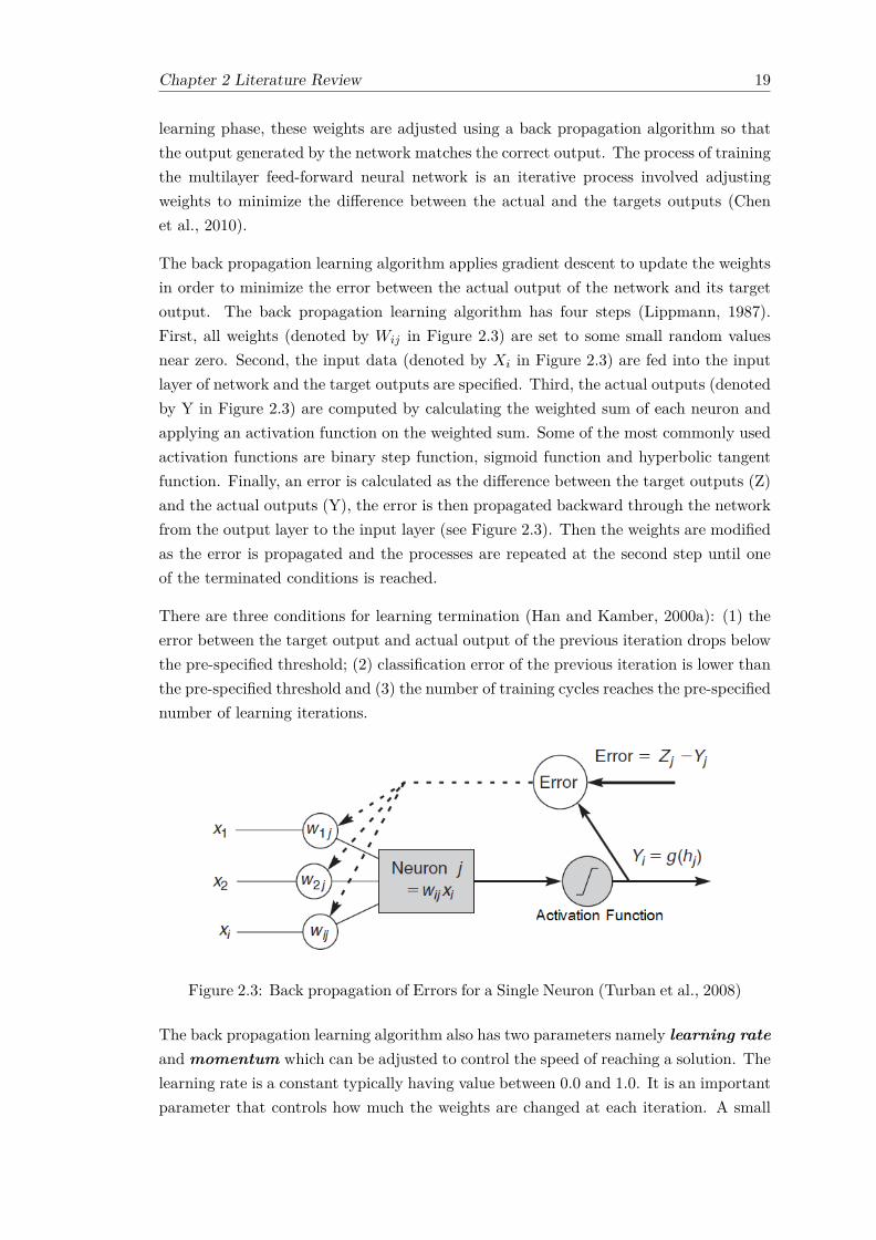
Chapter 2 Literature Review 19
learning phase, these weights are adjusted using a back propagation algorithm so thatthe output generated by the network matches the correct output. The process of trainingthe multilayer feed-forward neural network is an iterative process involved adjustingweights to minimize the difference between the actual and the targets outputs (Chenet al., 2010).
The back propagation learning algorithm applies gradient descent to update the weightsin order to minimize the error between the actual output of the network and its targetoutput. The back propagation learning algorithm has four steps (Lippmann, 1987).First, all weights (denoted by Wij in Figure 2.3) are set to some small random valuesnear zero. Second, the input data (denoted by Xi in Figure 2.3) are fed into the inputlayer of network and the target outputs are specified. Third, the actual outputs (denotedby Y in Figure 2.3) are computed by calculating the weighted sum of each neuron andapplying an activation function on the weighted sum. Some of the most commonly usedactivation functions are binary step function, sigmoid function and hyperbolic tangentfunction. Finally, an error is calculated as the difference between the target outputs (Z)and the actual outputs (Y), the error is then propagated backward through the networkfrom the output layer to the input layer (see Figure 2.3). Then the weights are modifiedas the error is propagated and the processes are repeated at the second step until oneof the terminated conditions is reached.
There are three conditions for learning termination (Han and Kamber, 2000a): (1) theerror between the target output and actual output of the previous iteration drops belowthe pre-specified threshold; (2) classification error of the previous iteration is lower thanthe pre-specified threshold and (3) the number of training cycles reaches the pre-specifiednumber of learning iterations.
Figure 2.3: Back propagation of Errors for a Single Neuron (Turban et al., 2008)
The back propagation learning algorithm also has two parameters namely learning rateand momentum which can be adjusted to control the speed of reaching a solution. Thelearning rate is a constant typically having value between 0.0 and 1.0. It is an importantparameter that controls how much the weights are changed at each iteration. A small
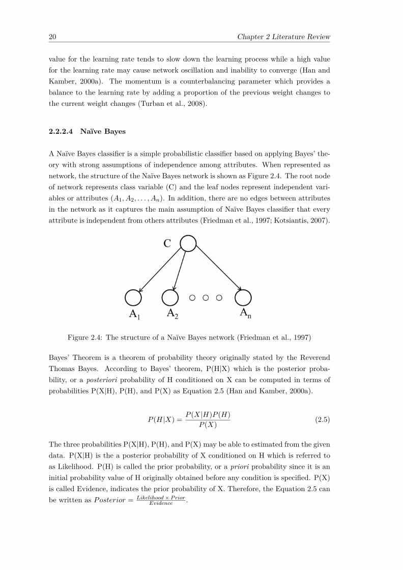
20 Chapter 2 Literature Review
value for the learning rate tends to slow down the learning process while a high valuefor the learning rate may cause network oscillation and inability to converge (Han andKamber, 2000a). The momentum is a counterbalancing parameter which provides abalance to the learning rate by adding a proportion of the previous weight changes tothe current weight changes (Turban et al., 2008).
2.2.2.4 Naïve Bayes
A Naïve Bayes classifier is a simple probabilistic classifier based on applying Bayes’ the-ory with strong assumptions of independence among attributes. When represented asnetwork, the structure of the Naïve Bayes network is shown as Figure 2.4. The root nodeof network represents class variable (C) and the leaf nodes represent independent vari-ables or attributes (A1, A2, . . . , An). In addition, there are no edges between attributesin the network as it captures the main assumption of Naïve Bayes classifier that everyattribute is independent from others attributes (Friedman et al., 1997; Kotsiantis, 2007).
Figure 2.4: The structure of a Naïve Bayes network (Friedman et al., 1997)
Bayes’ Theorem is a theorem of probability theory originally stated by the ReverendThomas Bayes. According to Bayes’ theorem, P(H|X) which is the posterior proba-bility, or a posteriori probability of H conditioned on X can be computed in terms ofprobabilities P(X|H), P(H), and P(X) as Equation 2.5 (Han and Kamber, 2000a).
P (H|X) =P (X|H)P (H)
P (X)(2.5)
The three probabilities P(X|H), P(H), and P(X) may be able to estimated from the givendata. P(X|H) is the a posterior probability of X conditioned on H which is referred toas Likelihood. P(H) is called the prior probability, or a priori probability since it is aninitial probability value of H originally obtained before any condition is specified. P(X)is called Evidence, indicates the prior probability of X. Therefore, the Equation 2.5 canbe written as Posterior = Likelihood× Prior
Evidence .

Chapter 2 Literature Review 21
In the context of classification problems, X is a data sample contained n attributesX1, X2, · · · , Xm with an unknown class label and H is a hypothesis that X belongs toclass C. The goal is to determine P(H|X), the probability that sample X belongs to classC, given the attribute description of X. Suppose that there are m classes, C1, C2, · · · , Cm.X will be labelled following to the class having the highest posterior probability, condi-tioned on X (Han and Kamber, 2000a).
Similar to other classification techniques, Naïve Bayes classification consists of trainingand testing phases. In the training phase, the distributions of P(H) and P(Xi|H) foreach attribute are computed from the training data. P(H) indicates the probability ofeach class Ci and is computed as the number of records with class Ci divided by thenumber of all training records. For the discrete input attributes, P(Xi|H) is computed asthe number of records of class Ci having attribute value u for Xi divided by the numberof records of class Ci. These computed probabilities form the conditional probabilitytables, the output of the training phase (Han and Kamber, 2000a).
Using the conditional probability tables, a class of new data X ′ can be predicted inthe training phase. The probabilities corresponding to the attribute value of X ′ inthe conditional probability tables are used to compute the posterior probability of eachclass Ci regarding Bayes’ theorem and then the class Ci having the highest posteriorprobability will be assigned as class of X ′ . Specifically, the posterior probability of eachclass Ci is calculated as the multiplication among the probability of input attributesP(X ′
i|Ci) and probability of class Ci since the independence assumption of Naïve Bayesis applied and the denominator of Bayes’ theorem has the same value for all classes,referred to as constant so it can be omitted from the formula.
The main advantage of Naïve Bayes is its simplicity which results in low computationalcomplexity. The training is very easy and fast using the empirical frequency and testingis straightforward - just looking up the conditional probability tables and performingprobability multiplication. In addition, it is capable of handling large data sets veryquickly and attains accurate results (Kotsiantis, 2007). Moreover, studies comparingclassification algorithms (Domingos and Pazzani, 1997) have shown that Naïve Bayesproduces higher accuracy than more sophisticated approaches including decision treeinduction, instance-based learning, and rule induction in many domains. The maindisadvantage of Naïve Bayes is its reliance on the assumption of independence amongattributes which is often unsatisfied with real data and causes the accuracy of NaïveBayes to be less than other more sophisticated techniques (such ANNs) (Kotsiantis,2007).

22 Chapter 2 Literature Review
2.2.2.5 Bayesian Networks
Bayesian Networks (BNs) known as belief networks, are directed acyclic graphs (DAG)with an associated set of probability tables (Heckerman, 1997). BNs consist of a qual-itative part which represents variables as nodes and relationships among variables asdirected edges in DAG, and a quantitative part which quantifies dependency intensitybetween variables in probabilistic terms (Ben-Gal, 2007). More specifically, for each vari-able (node) the probabilistic term is encoded in the conditional probability distributionthat quantifies the influences of its parent nodes. For discrete variables, the conditionalprobability distribution of non-root nodes is captured in table called conditional proba-bility tables (CPTs) which contain a local probability of node for each combination ofthe values of its parents whereas the conditional probability distribution of root nodes(the nodes without parents) depend solely on their probability distribution known as aprior probability distribution (Lee and Abbott, 2003).
Figure 2.5: The backache BN example adapted from (Ben-Gal, 2007). Eachnode represents variable with its conditional probability table.
The example of BNs shown in Figure 2.5 illustrates that backache might be caused bywrong sport activity or an uncomfortable chair. In this example, the node Chair andSport (denoted by C and S respectively) are the root nodes hence the probability tablesassociated with these nodes contain their prior probabilities. The nodes Back and Ache(denoted by B and A respectively) are the non-root nodes hence their CPTs containconditional probabilities for all possible value of their parents. For example, the parentnodes (C,S) of Back have two values (True, False) therefore the CPT of Back containsfour rows which each row represents probability of Back for each combination of valuesof node C and S.

Chapter 2 Literature Review 23
BNs can be used to compute the conditional probability of one node, given the values ofother nodes therefore BNs can be used as a classifier that predicts class value (dependentvariable) regarding the posterior probability distribution of the class node given the val-ues of input attributes (independent variables) (Cheng and Greiner, 2001). BNs improvethe performance of Naïve Bayesian classifiers by avoiding the independence assumption(Friedman et al., 1997) because BNs have an ability to capture the relationships amonginput variables which provides tremendous value in exploring data.
Applying Bayesian network techniques to classification consists of a training (learning)and a testing phase. The BNs learning involves a model construction and BNs testinginvolves a model inference for predicting class (Cheng and Greiner, 2001). Generally,there are two major tasks in BNs learning from data: structure learning and parameterlearning (Ben-Gal, 2007). The first aims to construct the DAG encoding the indepen-dencies among variables that are optimal for a given training data while the latter aimsto construct the CPTs for the learned network. The BN structure learning is consid-ered a harder problem than parameters learning since the number of possible structuresis extremely large; finding the optimal structure of BN from data is considered as anNP-hard problem (Khanteymoori et al., 2009). Further information about structurelearning can be found in Khanteymoori et al. (2009). The parameters learning task isestimating the conditional probability distribution of all nodes in the learned networkfrom the training data. According to Lee and Abbott (2003), in the case of no missingvalues in the training data, the parameter estimation can be done simply by using theempirical conditional frequencies from the data given the network structure, which issimilar to the probability computing involved in Naïve Bayes classification . In the casethat missing data exists, the algorithm for parameter estimating is used and the mostcommonly used algorithm is the Expectation Maximization (EM) algorithm.
The result of the learning phase is a learned network representing an approximation tothe probability distribution of all variables, and is used as a classifier to predict the classof the testing dataset in the testing phase. More precisely, the learned network is used tocompute the posterior probability of values of the target (class) variable given the valuesof the input variables in the testing dataset. After that, the class value that attains themaximum posterior probability is assigned as the class label of the instance in the testingdataset (Friedman et al., 1997). Note that, the conditional independence statementencoded in the BN network is exploited in computing the posterior probability. Thisconditional independence states that each variable is independent of its non-descendantsin the graph given the state of its parents. Thus, applying this statement provides anefficient way to compute the posterior probability by reducing the number of parametersneeded to characterize a joint probability distribution (Ben-Gal, 2007).
The BNs offers several advantages over other types of classification technique. The majoradvantages of BNs are (Heckerman, 1997; Lee and Abbott, 2003): (1) the graphicaldiagram of BNs provides a better understanding about the inter-relationships among

24 Chapter 2 Literature Review
the variables which help a human expert to be able to modify a BNs model to obtainbetter predictive model; (2) BNs have an ability to capture the relationships amonginput variables which provides tremendous value in exploring data and (3) BNs allowa human expert to add their knowledge related to a domain in the form of networktopology which contributes to the model efficiency; (4) BNs are flexible in handling themissing values and (5) BNs offer an efficient approach to avoid over fitting of data basedon probability theory. One of the limitations of BNs is the ability to deal with continuousdata thus this data has to be discretized before constructing BNs model (Nyberg et al.,2006).
2.3 Customer Satisfaction
Customer satisfaction has long been an area of interest in academic research and busi-ness practice, especially as it is postulated as one of the main indicators of businessperformance for the last decade. To provide a basic understanding about customersatisfaction, this section provides the review of customer satisfaction including the def-initions and importance of customer satisfaction, measuring and analysis of customersatisfaction, and research on mining customer satisfaction data.
2.3.1 Overview of customer satisfaction
Customer satisfaction is an evaluative judgement of quality and intensity that a productor service itself, or a feature of it, does fulfil expectations (Bosnjak, 2014). Customersatisfaction can also be defined as “person’s feeling of pleasure or disappointment whichresulted from comparing a product’s perceived performance or outcome against his/herexpectations”(Kotler and Keller, 2011). Many studies on customer satisfaction havebeen defined with different definitions of customer satisfaction as organisations attemptto measure it. Accordingly, Millán and Esteban (2004) summarized a list of customersatisfaction definitions which can be referred to for further reading.
The underlying concepts of the various definitions are that (1) satisfaction is a post-consumption evaluative judgement which is a comparison of perceived outcomes of prod-uct or service with expectations (Pizam et al., 2016). Accordingly, satisfaction with aproduct or service is a construct that requires experience and use of a product or service.As a matter of fact, the customer satisfaction is actually about consumer satisfactionrather than about buyer satisfaction; (2) satisfaction is a feeling. It is a temporaryattitude that can readily change given a group of circumstances (Hom, 2000). Hence,satisfaction is not a universal phenomenon and not every customer gets the same sat-isfaction out of the same product usage or service experience as he/she has differentneeds, objectives and personal experiences that influence his/her expectations (Pizamand Ellis, 1999).

Chapter 2 Literature Review 25
In an increasingly competitive environment, customer orientation is essential in manybusinesses (Dejaeger et al., 2012). Accordingly, customer satisfaction has been gettingimportance in business practices especially for the last decade. It is postulated as one ofthe main indicators of business performance (Mihelis et al., 2001) as measuring customersatisfaction provides a reflection of an organisation’s business activities. In addition,measuring customer satisfaction also provides meaningful and objective feedback aboutcustomer preferences and expectations which is useful for organisations in adjusting theiroperations and marketing to meet the customer needs and expectations.
The supporting evidence for the importance of customer satisfaction is that customersatisfaction measurements on a national scale such as the American Customer Satis-faction Index (ACSI)2 which was established in 1994 to provide information regardingcustomer satisfaction with the quality of household products and services available toU.S. consumers (Fornell et al., 1996). Following the same line, several countries have de-veloped the national measure of customer satisfaction for their own national economiessuch as the UK Customer Satisfaction Index (UKCSI)3, South African Customer Sat-isfaction Index (SAcsi)4 and Indian Customer Satisfaction Index (ICSI)5, etc. Thesemeasurements of customer satisfaction on a national scale provide uniform and compa-rable information that allows for systematic benchmarking over time and across firms.
Furthermore, customer satisfaction is considered as one key to customer retention (Kotlerand Keller, 2011) as a number of studies suggested that it positively influences on cus-tomer retention (Cengiz, 2010). A high level of satisfaction (with pleasurable experi-ences) is very likely to result in customer retention, product repurchase and the spreadof positive word-of-mouth. In contrast, a very low level of satisfaction (with unpleasur-able experiences) is very likely to result in abandoning the firm and even the spread ofnegative word (Kotler and Keller, 2011).
2.3.2 Measuring customer satisfaction
As previously explained, measuring customer satisfaction provides useful informationon how an organisation delivers a product or service to the marketplace. In order tomeasure customer satisfaction, customer satisfaction surveys and questionnaires are usedto determine customer attitudes and perceptions of the quality of the product or service.
Typically, in a social science context, satisfaction is referred to as a latent variable asit cannot be directly measured whereas variables that can be directly measured suchas sex, age, weight are called manifest variables (Kenett and Salini, 2012, p.3). Thelatent variable is indirectly measured through a number of manifest variables. Each
2http://www.theacsi.org/3https://www.instituteofcustomerservice.com4http://www.sacsi.co.za/5http://www.icsi.org.in/

26 Chapter 2 Literature Review
manifest variable refers to one specific aspect of the latent variable. Taking the numberof manifest variables together yields a meaning to the latent variable and builds thecontents of the latent variable (Cassel, 2006).
Therefore, in order to design a customer satisfaction questionnaire, a set of manifestvariables must be identified (Kenett and Salini, 2012, p.3) and these variables are usu-ally formulated as a set of questions in the questionnaire (Figini and Giudici, 2007).Accordingly, for a questionnaire design, each component or attribute that is relevantfor explaining the overall customer satisfaction should contain at least three questions(Cassel, 2006).
For example, in order to assess customer satisfaction in the private bank sector, it isnecessary to identify attributes that characterize this type of service and then identifya list of questions for each attribute. According to Mihelis et al. (2001), some possibleattributes of the bank sector are personnel of the bank, products, image of the bank, ser-vice and access. The possible questions attached to the attribute named personnel of thebank include all the characteristics concerning personnel such as skills and knowledge,responsiveness, communication and collaboration with customers, and friendliness.
Although satisfaction is best measured on a continuous scale, a Likert numeric scale iscommonly used to measure satisfaction both in academic and business practice (Allenand Wilburn, 2002; Kenett and Salini, 2012, p.58). The value of scales is limited andit represents the degree of satisfaction perceived by the customer, which is typicallyranges from the lowest point on the scale (representing the case when a customer is notsatisfied at all) to the highest point (representing the case when a customer is completelysatisfied).
In order to use the Likert scale, the choice of measurement scales has to be considered.The range of possible responses for a scale can vary and there has been much debate onan optimal number of responses. By now, five to seven-point scales are well establishedfor closed-questions (Fink, 2003, p.57), (Kenett and Salini, 2012, p.137). The five‐pointscale is typically used although there are arguments in favour of the seven‐point scale(Jamieson et al., 2004).
By using the Likert scale, responses are considered as ordinal data (Fink, 2003, p.52)which means that the response levels have a rank order and the interval between pointson the Likert scale cannot be assumed equal (Jamieson et al., 2004). For example, noone can say that the distances between ‘Completely satisfied’ and ‘Satisfied’ is the sameabout the distances between ‘Satisfied’ and ‘Neither satisfied or dissatisfied’.
Despite the fact that Likert-derived data is ordinal, it has become a common practiceto treat ordinal scales as interval scales. Hence, it is possibly to employ parametric testsinstead of non-parametric tests in analysis Likert-derived data. However, the researcher

Chapter 2 Literature Review 27
should consider the sample size and data distribution in determining whether parametricor non-parametric tests could be used to analyse such data (Jamieson et al., 2004).
2.3.3 Analysis of Customer satisfaction data
General data analysis techniques of customer satisfaction are statistical techniques suchas descriptive statistics, regression and correlation analysis. Some advanced and moderntechniques for analysis customer satisfaction data are Structural Equation Modelling(SEM), Bayesian Networks (BNs), etc.
2.3.3.1 Descriptive statistics
Descriptive statistics are the basic measures used to summarize and describe satisfactionsurvey data. The reporting of descriptive statistics generally consists of the percentageof individuals choosing a particular response to each question on a survey, measuresof central tendency (such as the mean, median and mode), and measures of dispersion(such as the standard deviation, the variance, and the standard error) which describethe variability of response data (Goff et al., 2002).
Additionally, the reporting of descriptive statistics also includes a graphical display ofdata in the form of charts and graphs which facilitates an identification of patterns inthe data. Commonly used charts and graphs are bar chart, pie chart and histogram.Note that the choice of descriptive statistics is dependent on the type of data beingobserved. Further detail about descriptive statistics can be found in (Field, 2009, p.31-60; p.87-130).
While descriptive statistics provide some information that can be used during the pre-liminary analysis or used in conjunction with some advance statistics, they are not ableto provide an in depth analysis of customer satisfaction (Grigoroudis and Siskos, 2009, p.28) (such as key driver analysis). Therefore, an analysis of customer satisfaction shouldnot stop at this analysis level.
2.3.3.2 Statistical and modern approaches
Multiple linear regression (MLR) is one of the most widely used statistical techniquesfor analysing customer satisfaction data. The technique is used to determine which at-tributes of product or service are the key drivers of customer satisfaction by discoveringthe relationship between the satisfaction/performance of the set of attributes (indepen-dent variables) and the overall customer satisfaction judgement (dependent variable)(Grigoroudis and Siskos, 2009, p.28). An overview of MLR has already been providedin Section 2.2.2.

28 Chapter 2 Literature Review
One statistical technique that can be used to determine key driver attributes is corre-lational analysis. Key driver attributes are those that are most closely associated withoverall satisfaction. Further detail about correlation can be found in (Field, 2009, p.166-196).
Another statistical technique widely used in analysing customer satisfaction data isfactor analysis. Its most common application is the reduction of a large number ofattributes in the steps of designing a customer satisfaction survey.
Apart from these basic statistical techniques, some advance techniques for analysis cus-tomer satisfaction data are SEM which is a statistical technique for measuring relation-ships among latent variables (Grigoroudis and Siskos, 2009, p.34-40), conjoint analysiswhich is used to assess the effects of the trade-offs made by customers, when they eval-uate their satisfaction for a particular product or service (Grigoroudis and Siskos, 2009,p.41). Additionally, there are some modern techniques in customer satisfaction dataanalysis such as BNs, CUB models and Rasch model. Details of these techniques canbe found in (Kenett and Salini, 2012, p.193-213; p.231-279).
2.3.4 Research on mining customer satisfaction data
To gain better insight into customer satisfaction in various domains, some researchershave started applying data mining techniques in analysis of customer satisfaction data.Through the literature review, the summary of 10 publications is presented in Table 2.2.With regard to this table, the main objective of these previous works is to investigatewhich data mining technique offers the best predict customer satisfaction. Thus, the listof observed techniques and the evaluation metric are provided in these works.
The majority of the previous works conducted a comparison between the combination oftwo data mining techniques such as neural network, ordinal logistic regression (OLR),multiple linear regression (MLR), decision tree and Bayesian networks (BNs). An ex-ception was the works by Azzalini et al. (2012), Dejaeger et al. (2012) and Nikolaos(2009) which conducted a comparison among three or more techniques.
Azzalini et al. (2012) conducted the comparison of eight data mining techniques in whichsome additional selected techniques are k-nearest neighbour, support vector machine,bagging trees and random forests. Dejaeger et al. (2012) conducted the comparison offour data mining techniques: OLR, neural network, decision tree and support vectormachine (SVM). Nikolaos (2009) conducted the comparison of two data mining tech-niques namely neural networks and rule-induction with the other techniques in the fieldof customer satisfaction analysis namely Rough set and Multi-criteria decision analysis.
The common evaluation metrics used for comparing between or among the techniquesare misclassification rate (the ratio of number of samples that are incorrectly classified to
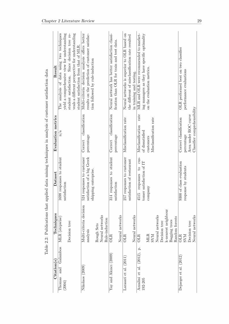
Chapter 2 Literature Review 29
Table2.2:
Publications
that
appliedda
taminingtechniqu
esin
analysis
ofcustom
ersatis
factionda
ta
Citation(s)
Techniqu
esDataset
Evaluationmetrics
Result
Tho
mas
and
Galam
bos
(200
4)MLR
(stepw
ise)
1698
respon
sesto
stud
ent
satis
faction
n/a
The
analysis
ofda
tausing
two
techniqu
esyieldacompreh
ensiv
eview
forun
derstand
ing
Decision
tree
stud
entsatis
faction.
Sinc
ede
cisio
ntree
re-
vealsa
diffe
rent
perspe
ctiveforu
nderstan
ding
stud
entsatis
factionfro
mthat
ofMLR
.Nikolao
s(200
9)Multi-
crite
riade
cisio
nan
alysis
524respon
sest
ocu
stom
ersatis
factionof
abigGreek
shipping
enterpris
e.
Correct
classifi
catio
npe
rcentage
Multi-
crite
riade
cisio
nan
alysis
offersbe
tter
results
onthepred
ictio
nof
custom
ersatis
fac-
tionfollo
wedby
rule-in
duction
Rou
ghSe
tsNeu
raln
etwo
rks
Rule-indu
ction
Yayan
dAkınc
ı(20
09)
OLR
314
respon
sesto
stud
ent
satis
faction
Correct
classifi
catio
npe
rcentage
Neu
raln
etwo
rkha
sbe
tter
satis
factionclassi-
ficationthan
OLR
fortrainan
dtest
data.
Neu
raln
etwo
rks
Larasatiet
al.(
2011
)OLR
257respon
sest
ocu
stom
ersatis
factionof
restau
rant
Misc
lassificatio
nrate
Neu
raln
etwo
rksis
supe
riorto
OLR
basedon
thediffe
rent
ofmisc
lassificatio
nrate
resulte
dNeu
raln
etwo
rks
intraining
andtesting.
Azzaliniet
al.(201
2),p.
192-20
5OLR
4515
respon
ses
tocu
s-tomer
satis
factionof
ITMisc
lassificatio
nrate
ofdissatisfi
edMLR
andOLR
were
recommen
dedto
market-
ingman
agersas
they
have
specificop
timality
MLR
compa
nycu
stom
ers
ontheevalua
tionmetric
s.SV
MMisc
lassificatio
nrate
Neu
raln
etwo
rks
Decision
tree
k-ne
arestne
ighb
our
Bagg
ingtrees
Ran
dom
forests
Dejaegeret
al.(
2012)
OLR
9300
ofclassevalua
tion
Correct
classifi
catio
nOLR
perfo
rmed
best
ontw
oclassifi
erSV
Mrespon
seby
stud
ents
percentage
perfo
rman
ceevalua
tions
Decision
tree
Areaun
derR
OCcu
rve
Neu
raln
etwo
rks
Classifier
compreh
ensib
ility

30 Chapter 2 Literature Review
Table2.2
(cont):Publications
thatapplied
datamining
techniquesin
analysisofcustom
ersatisfaction
data
Citation(s)
TechniquesDataset
Evaluation
metrics
Result
Huang
(2012)OLR
425responsesto
customer
satisfactionoffour
hotelsCorrect
classificationpercentage
Neuralnetwork
ismore
suitablethan
OLR
forpredicting
customer
satisfactionand
Neuralnetworks
inTaiwan
repurchasebehaviour.
Klicek
etal.(2014)
BNs
239responsesto
customer
satisfactionofa
streetCorrect
classificationpercentage
Acom
binationmodelofthe
twotechniquesis
ableto
predictcustom
ersatisfaction
onthe
Neuralnetworks
festivalhigh
levelofaccuracy.Perucca
andSalini(2014)
OLR
World
Bank’sRailways
Misclassification
rateBN
sis
superiorto
OLR
basedon
theBN
sdatabase.
misclassification
ratetested
byusing
cross-validation.
Tama(2015)
Neuralnetworks
340responsesto
customer
satisfactionoffast-food
Correct
classificationpercentage
Neuralnetwork
hasbetter
satisfactionclassi-
ficationthan
decisiontree.
Decision
treerestaurant

Chapter 2 Literature Review 31
the total number of samples) and correct classification percentage (the ratio of numberof samples that are correctly classified to the total number of samples multiplied by100). The best predicting customer satisfaction technique is the one with the lowestmisclassification rate or the one with highest correct classification percentage.
For a comparison of results among data mining techniques, Yay and Akıncı (2009),Larasati et al. (2011) and Huang (2012) reported that neural network is superior to OLRin predicting customer satisfaction. This contradicts the results of Azzalini et al. (2012)and Dejaeger et al. (2012) which reported that OLR is superior to neural networks andthe other techniques such as decision tree and SVM in predicting customer satisfaction.
Consider the comparison results of the other two works by Perucca and Salini (2014)and Tama (2015) which compared different sets of the techniques from the previouslystated works. The first reported that BNs is superior to OLR in predicting customersatisfaction, while the latter reported that neural network is superior to decision treein predicting customer satisfaction. In addition, the work by Nikolaos (2009) reportedthat Multi-criteria decision analysis offers better results on the prediction of customersatisfaction followed by the rule-induction.
The rest of the publications by Thomas and Galambos (2004) and Klicek et al. (2014) didnot directly compared the two data mining techniques using evaluation metrics thereforethe comparison results were not reported. In their work, Thomas and Galambos (2004)investigated the rules generated from linear regression and decision tree on studentsatisfaction data and concluded that the analysis of data using these two techniquesyielded a comprehensive view for understanding student satisfaction. Klicek et al. (2014)proposed an approach to combine BNs with neural networks in predicting customersatisfaction. Specifically, BNs was used as a feature selection technique to reduce thenumber of input variables of the neural network. Based on the correct classificationpercentage, Klicek et al. (2014) reported that a hybrid technique was able to predictcustomer satisfaction at a high level of accuracy (over 90%).
These past studies of mining customer satisfaction focused on building a model to predictthe customer satisfaction. They did not provide further steps for deriving importance,which is the main component of IPA, from the models of data mining techniques. Thepoint of interest drawn from these studies is that data mining is a promising tool todiscover some useful information from customer satisfaction data. These past studiesalso suggested some interesting data mining techniques which are neural network, BNs,decision tree and SVM that could be used to analyse and estimate importance fromcustomer satisfaction data. In another word, the review of the past studies raised theidea of introducing new data mining techniques in the field of IPA studies.

32 Chapter 2 Literature Review
2.4 Summary
In this chapter, three principal topics relating to the research are described namely– SWOT analysis, data mining and customer satisfaction. First, SWOT analysis isreviewed to examine the state of the art of the SWOT approach. The overview ofSWOT analysis shows that this simple method is important as part of strategic planning.It supports companies to gain better insight into their internal and external businessenvironments enabling them to generate good plans to achieve their business goals. Themain advantage of SWOT analysis is its simplicity which has resulted in its continueduse since the 1960s. Despite its advantage, there are typical shortcomings existing inthe SWOT approach as it produces a superficial and imprecise list of factors, relies onsubjective perception of a company’s staff and lacks factor prioritization regarding theimportance of each SWOT factor. Due to the disadvantage in prioritization of SWOTfactors, a number of researchers proposed new variations of SWOT approaches thatintegrated SWOT with others quantitative methods such as AHP-SWOT, FAHP-SWOTand ANP-SWOT. These approaches make SWOT factors commensurable regarding theirrelative importance. However, both the quantitative SWOT and traditional SWOTapproaches do not take customers’ points of view into consideration even if it can ensurethat the capabilities perceived by a company are recognized and valued by the customers.Therefore, this research aims to fill this gap in previous SWOT approaches. In term ofthe literature about the SWOT analysis system, techniques for developing the SWOTanalysis system are mainly expert systems, text mining and sentiment analysis.
Data mining is the core step of KDD which aims to extract useful knowledge from ahuge amount of data. Data mining relies on the disciplines of statistics and of machinelearning in data analysis. Data mining methods can be divided in two groups: predic-tion and description. The predictive data mining method infers the extracted patternof current data to predict the pattern of future data. Examples of predictive data min-ing methods are Classification and Regression. The descriptive data mining methodexploits extracted patterns for describing common characteristics of data. Examples ofdescriptive data mining methods are Clustering and Association rule discovery. Thisreport is mainly focused on methods of prediction and classification technique namely –MLR, OLR, BPNN, Naïve Bayes and BNs that will be applied to customer survey datato determine the company’s attribute importance. For each technique, steps for trainingand testing classification or prediction model are described along with its advantagesand disadvantages.
Customer satisfaction has long been an area of interest in academic research and busi-ness practice and has been getting importance in business practices especially for thelast decade. Measuring customer satisfaction provides meaningful and objective feedback

Chapter 2 Literature Review 33
about customer preferences and expectations which is useful for organisations in adjust-ing their operations and marketing to meet the customer needs and expectations result-ing in a competitive advantage. Typically, customer satisfaction is measured throughthe questionnaires using closed-ended or open-ended questions. This report is mainlyfocused on measuring customer satisfaction on a Likert scale through the closed-endedquestions. Therefore, techniques for analysis customer satisfaction that were examinedare basic statistical techniques such as descriptive statistics, regression analysis and someadvanced statistical techniques such as SEM and conjoint analysis. In addition to thestatistical techniques, many researchers have started applying data mining techniquesto the analysis of customer satisfaction data with the aim of gaining better insight intocustomer satisfaction. A review of past research on mining customer satisfaction datashowed that data mining techniques such as neural network, BNs, decision tree andSVM are promising techniques for discovering some useful information from customersatisfaction data.


Chapter 3
Importance-Performance Analysis
To provide additional background to the research, this chapter explains about Importance-Performance Analysis (IPA). The chapter begins with an overview of IPA (Section 3.1)where the main focus is the approaches that have been used for measuring importance.Section 3.2 provides the past comparative studies of method for measuring importancefollowed by the methodology for deriving importance by using well-known data miningtechniques, Section 3.3.
3.1 Overview of Importance-Performance Analysis
Importance-Performance Analysis (IPA) is a technique proposed by Martilla and James(1977) for analysing customer satisfaction towards a company’s product or service . Fordecades, IPA has been used as a tool for understanding customers’ needs and desires soas to develop marketing strategies to respond to them. In a nutshell, IPA measures thesatisfaction based on two components: ‘performance’ and ‘importance’. The intersectionof these two components creates a two-dimensional matrix that helps a company toidentify improvement opportunities by discovering the attributes of a company’s productor service that should be maintained or improved based on the customers’ viewpoints(Garver, 2003).
IPA is widely used in many areas in which customer satisfaction is a key to a thriv-ing business including higher education (Ford et al., 1999; Kitcharoen, 2004; Silva andFernandes, 2012), tourism (Tarrant and Smith, 2002; Luo et al., 2010; Taplin, 2012a),government service (Seng Wong et al., 2011), health service (Gonçalves et al., 2014) ,convenience store (Shieh and Wu, 2009) and banking service (Wu et al., 2012).
The advantage of IPA is based on its simplicity and ease of use. IPA provides an intuitiveway to indicate strategic actions to be taken with respect to each attribute of a company’sproduct or service (Tarrant and Smith, 2002). One of the major shortcomings of IPA
35

36 Chapter 3 Importance-Performance Analysis
(as it is a model in quadrants) is that a slight change in the position of an attributewill likely result in identifying dramatically different attributes for improvement (Bacon,2003).
This shortcoming of IPA is related to two methodological issues of IPA which are I-P mapping partitions and direct vs. indirect measurement of importance (Lai andHitchcock, 2015; Sever, 2015). The first issue is about approaches for identifying cut-off points of importance and performance that divide the IPA space. Further detailregarding this issue will be discussed in sub-section 3.1.2
The second issue is associated with the argument whether importance should be directlyobtained from customer or indirectly derived on the basis of performance and overallcustomer satisfaction. Note that only the second issue is being focused and defined asthe research question of this thesis. Further detail regarding the current approaches formeasuring importance is explained in sub-section 3.1.4
3.1.1 IPA matrix
Since customer satisfaction is a function of customer perceptions, it involves the qualityof the company’s product or service and customer expectations. Therefore, IPA measuresthe satisfaction from customer satisfaction surveys based on two components of productor service attributes: the importance of a product or service to a customer and theperformance of a company in providing that product or service (Martilla and James,1977).
The intersection of these two components creates a two-dimensional matrix (Figure 3.1)where the importance is shown by the x-axis and the performance of the company bythe y-axis.
Depending on cell location, the attributes related to a company’s product or service areconsidered as major or minor strengths and weaknesses. The four quadrants in IPA arecharacterized by Silva and Fernandes (2010) as:
Quadrant 1. Keep up with the good work (high importance, high perfor-mance): this cell contains attributes that are perceived to be very importantto customers, and the company seems to provide high levels of performance inthese attributes. Thus these attributes are referred to as the major strengths andopportunities for achieving or maintaining competitive advantage;
Quadrant 2. Possible overkill (low importance, high performance): this cellcontains attributes that are perceived as of low importance to customers, but thecompany seems to provide high levels of performance in these attributes. Thusthese attributes are referred to as the minor strengths implying that resources

Chapter 3 Importance-Performance Analysis 37
Figure 3.1: The IPA matrix (Hosseini and Bideh, 2013)
committed to factor in this quadrant would be better used in other quadrants inneed of improved performance;
Quadrant 3. Low priority (low importance, low performance): this cell con-tains attributes that are rated as of low importance and low performance. Thusthese attributes are referred to as the minor weaknesses that do not require a greatdeal of priority for improvement;
Quadrant 4. Concentrate here (high importance, low performance): thiscell contains attributes that are perceived to be very important to customers butperformance levels are fairly low. Thus these attributes are referred to as the majorweaknesses that require immediate attention for improvement.
This IPA matrix facilitates the company to prioritize the product or service’s attributesthat need to be of concern in order to satisfy their customers. For example, the productor service’s attributes that are indicated as major weaknesses (Quadrant 4) should re-ceive top priority and be the focus of improvement efforts. In contrast, the product orservice’s attributes considered as major strengths (Quadrant 1) should be maintainedand leveraged to ensure that the company continues to deliver good performance in theseareas (Garver, 2003). Additionally, the IPA result can be interpreted as major/minorstrengths and weaknesses (Deng et al., 2008a; Silva and Fernandes, 2012; Hasoloan et al.,

38 Chapter 3 Importance-Performance Analysis
2012; Hosseini and Bideh, 2013). Therefore, the IPA approach can be used to analysecustomer surveys for SWOT analysis.
3.1.2 Developing the IPA matrix
Generally, data regarding customers’ perceptions toward a company’s product or ser-vice gathered via customer satisfaction surveys are analysed for constructing an IPAmatrix. According to Duke and Mount (1996), the steps for developing an IPA matrixare described and shown in Figure 3.2.
Figure 3.2: Steps for constructing IPA matrix
Step 1. Determine attributes to be measured: This is a critical step for conduct-ing IPA since the usefulness of IPA will be severely limited, if evaluative factorsimportant to the customer are overlooked. Typically, this attributes list is basedon a thorough literature review in each application area or by interviews (Martillaand James, 1977).
Step 2. Create questionnaire and conduct customer survey: The product orservice’s attributes identified in the previous step are then used to develop ques-tionnaires. Typically, the questionnaires contain questions that ask customers to

Chapter 3 Importance-Performance Analysis 39
rate the importance of the attribute ranging from “not important at all” to “highlyimportant” and the performance of the attribute ranging from “very dissatisfied”to “very satisfied” in a 5-point or 7-point Likert scale. Next, the questionnairesare then administered to customers for obtaining their response on a product orservice (Skok et al., 2001).
Step 3. Obtaining importance and performance: performance is typically cal-culated on a rating scale whereas importance can be calculated either on a ratingscale (self-stated importance) or estimated on the basis of performance (implicitlyderived importance) (Oliver,1997) as cited in (Eskildsen and Kristensen, 2006). Intraditional IPA, both importance and performance are measured based on customerrating scales (Martilla and James, 1977). Other variations of IPA applied differentmethods to measure the importance and performance which will be described inthe next sections.
Step 4. Plot importance and performance on matrix: Through this step, oneof the approaches of I-P mapping partitions is identified to set the cut-off pointsthat divide the IPA space into areas of different priorities. Then the identifiedattributes are plotted against each other, allowing the analyst to examine theattributes located in each area for generating an action plan.
Generally, there are three I-P mapping approaches that could be used to par-tition the IPA space: scale-centred quadrants approach, data-centred quadrantsapproach and diagonal line approach (Bacon, 2003). A scale-centred quadrantsapproach use the midpoint of the measurement scale as the cut-off points (e.g.the value of 3 on the 5-point Likert scale) (Garver, 2003) whereas a data-centredquadrants approach use either aggregate averages or median value of importanceand performance as the cut-off points.
In a diagonal line approach, an upward 45◦ diagonal line is used to partition theIPA space (Bacon, 2003). All attributes located on the diagonal line have equalpriorities for improvement since their importance is equal to performance (I =
P ). In case the x-axis represents importance and y-axis represents performance,attributes located above the diagonal line depict that their importance is less thanperformance (I < P ); hence, they have the lower priorities for improvement thanattributes located below the diagonal line (I > P ).
In addition to these three approaches of I-P mapping partitions, Sever (2015)suggested the possible improvement of I-P mapping partitions by applying receiveroperating characteristic (ROC) for evaluating and selecting optimal cut-off pointsof importance and performance.
As the majority of researchers use the data-centred quadrant for dividing the IPAspace (Sever, 2015), this study will employ this approach for dividing the IPAspace. Specifically, cut-off points on the x-axis and y-axis are defined as aggregate
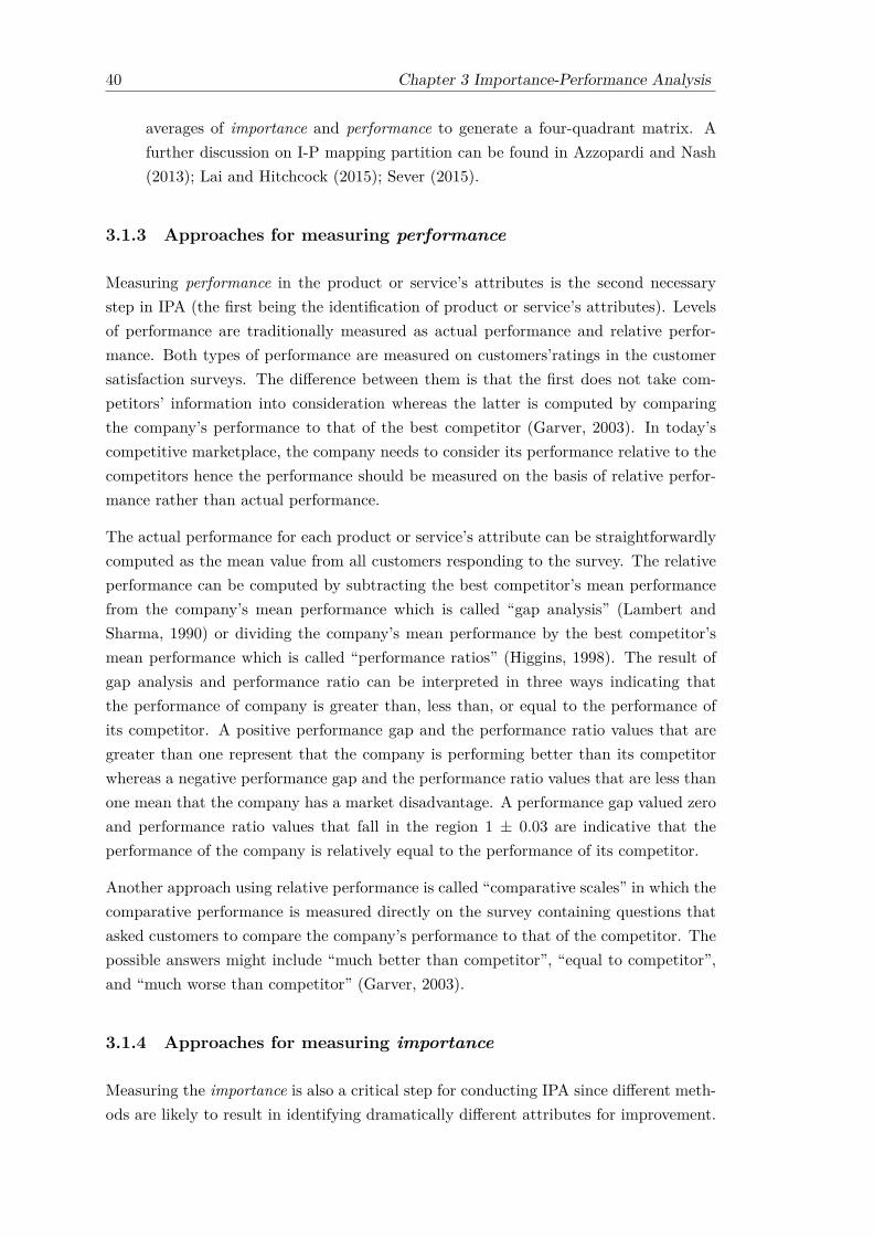
40 Chapter 3 Importance-Performance Analysis
averages of importance and performance to generate a four-quadrant matrix. Afurther discussion on I-P mapping partition can be found in Azzopardi and Nash(2013); Lai and Hitchcock (2015); Sever (2015).
3.1.3 Approaches for measuring performance
Measuring performance in the product or service’s attributes is the second necessarystep in IPA (the first being the identification of product or service’s attributes). Levelsof performance are traditionally measured as actual performance and relative perfor-mance. Both types of performance are measured on customers’ratings in the customersatisfaction surveys. The difference between them is that the first does not take com-petitors’ information into consideration whereas the latter is computed by comparingthe company’s performance to that of the best competitor (Garver, 2003). In today’scompetitive marketplace, the company needs to consider its performance relative to thecompetitors hence the performance should be measured on the basis of relative perfor-mance rather than actual performance.
The actual performance for each product or service’s attribute can be straightforwardlycomputed as the mean value from all customers responding to the survey. The relativeperformance can be computed by subtracting the best competitor’s mean performancefrom the company’s mean performance which is called “gap analysis” (Lambert andSharma, 1990) or dividing the company’s mean performance by the best competitor’smean performance which is called “performance ratios” (Higgins, 1998). The result ofgap analysis and performance ratio can be interpreted in three ways indicating thatthe performance of company is greater than, less than, or equal to the performance ofits competitor. A positive performance gap and the performance ratio values that aregreater than one represent that the company is performing better than its competitorwhereas a negative performance gap and the performance ratio values that are less thanone mean that the company has a market disadvantage. A performance gap valued zeroand performance ratio values that fall in the region 1 ± 0.03 are indicative that theperformance of the company is relatively equal to the performance of its competitor.
Another approach using relative performance is called “comparative scales” in which thecomparative performance is measured directly on the survey containing questions thatasked customers to compare the company’s performance to that of the competitor. Thepossible answers might include “much better than competitor”, “equal to competitor”,and “much worse than competitor” (Garver, 2003).
3.1.4 Approaches for measuring importance
Measuring the importance is also a critical step for conducting IPA since different meth-ods are likely to result in identifying dramatically different attributes for improvement.

Chapter 3 Importance-Performance Analysis 41
Two different methods that are commonly used for estimating importance of attributesin IPA are customers’ self-stated importance (explicit) and statistically inferred impor-tance (implicit).
The customers’ self-stated approach asks survey respondents to rate the importance ofeach product or service’s attribute and calculates importance based on customer prefer-ence (e.g. rating scale, partial ranking). Although it is a commonly used approach, thismethod has some limitations. Primarily, adding questions for asking customers to rateimportance increases the survey length which might affect the response rates (Garver,2003). Secondly, self-stated importance tends to have low discrimination power as cus-tomers tend to consider that all attributes are very important (Gustafsson and Johnson,2004).
Additionally, Matzler et al. (2004) stated that the traditional IPA has two assumptionsthat are erroneous in practice: (1) Attribute performance and attribute importance aretwo independent variables. (2) The relationship between attribute performance and over-all performance is linear and symmetric. They pointed out that many researchers haveproved that the relationship between attribute performance and attribute importanceis causal which means changes in performance lead to changes in importance (Sampsonand Showalter, 1999; Matzler et al., 2004) and the relationship between attribute per-formance and overall customer satisfaction (performance) is asymmetrical (Kano et al.,1984; Matzler and Sauerwein, 2002). Since these assumptions are erroneous in the realworld, many researches argued that the customers’ self-stated importance is not anadequate method to measure importance (Matzler et al., 2003; Deng et al., 2008b).
Consequently, the statistically inferred importance is introduced as a method to mea-sure the importance by deriving the relationships between attributes’ performances andoverall performance measures such as overall satisfaction (Garver, 2003; Tontini andSilveira, 2007; Pezeshki et al., 2009). The different statistical methods for deriving im-portance measures are multiple regression analysis (MLR) (Matzler and Sauerwein, 2002;Pezeshki et al., 2009; Ho et al., 2012), ordinal logistic regression (OLR) (Larasati et al.,2011), structural equation models (SEMs) or partial correlation (Matzler et al., 2003;Deng et al., 2008b; Ban and Bogdan, 2013).
In regression analysis- MLR and OLR, an entire set of attributes’ performance (in-dependent variables) are regressed against the overall customer satisfaction (dependentvariable). According to this method, the regression coefficients are considered as implicitimportance which expresses the influence of product or services’ attributes on the over-all satisfaction. The higher the regression coefficients of attributes, the more importantthey are in customers’ opinion (Pezeshki et al., 2009). SEMs are multivariate regres-sion models in which each structural equation represents the cause-effect relationshipsamong variables in the model. The structural parameters in the models can be estimatedby a maximum likelihood (ML) model or partial least squares (PLS) (Gustafsson and

42 Chapter 3 Importance-Performance Analysis
Johnson, 2004; Huang et al., 2007). These structural parameters indicate the effects ofthe attributes on the overall satisfaction. For partial correlation, the importance of theattributes is determined through the partial correlation coefficient by correlating eachattribute’s performance with overall satisfaction (Ban and Bogdan, 2013). Specifically,the correlation coefficient is a measure of the linear dependence between one attribute’sperformance (independent variable) and overall satisfaction (dependent variable) whenother attribute’s performances are eliminated.
The IPA is sensitive to the importance measurements employed as shown in an empiricalstudy of the two importance measurements (stated and statistically inferred approach)conducted by Matzler et al. (2003). In this empirical study, the importance of an indi-vidual attribute, which was assessed by two forms of customers’ self-stated importance(partial ranking and rating scale) are compared to the importance measured by statis-tically derived importance (correlation analysis). The results of this paper showed thatthe results from both methods are different and demonstrated that classical IPA (self-stated importance) could be misleading, since the self-stated method does not considerthe relationship between attribute importance and overall satisfaction. Another empir-ical study on the importance measurements drawn by Musa et al. (2010) also reportsthat the difference of IPA results depended on how the importance is measured.
Although the statistically inferred importance is superior to the self-stated importance(Chu, 2002), the use of these statistical methods depends on some underlying assump-tions that are always violated in the real world (Garver, 2003). First, data are relativelynormal and second, the relationships between independent and dependent variables arelinear. Additionally, both multiple regression analysis and structural equation modelshave another limitation that is the collinearity between the attributes (multicollinear-ity). The presence of multicollinearity can result in reducing the effects of the individualattributes on overall satisfaction (Hanson, 1992) which may lead to misleading and un-usual results.
Recently, data mining techniques such as Artificial Neural Networks (ANNs) have be-come an alternative method for determining importance. ANNs implicitly detect com-plex non-linear relationships between independent (attributes’ performance) and de-pendent variables (overall satisfaction). Moreover, ANNs are capable of dealing withcollinearity between the independent variables. Since ANNs overcome limitations oftraditional statistics, ANNs are a more suitable method to derive importance than sta-tistical methods which can be biased and misleading (Deng et al., 2008a). For example,Krešić et al. (2013) conducted an empirical study that compares three methods for de-riving importance namely correlation, multiple linear regression and back-propagationneural networks (BPNN). This study revealed that BPNN has superior predictive valid-ity than multiple linear regression.
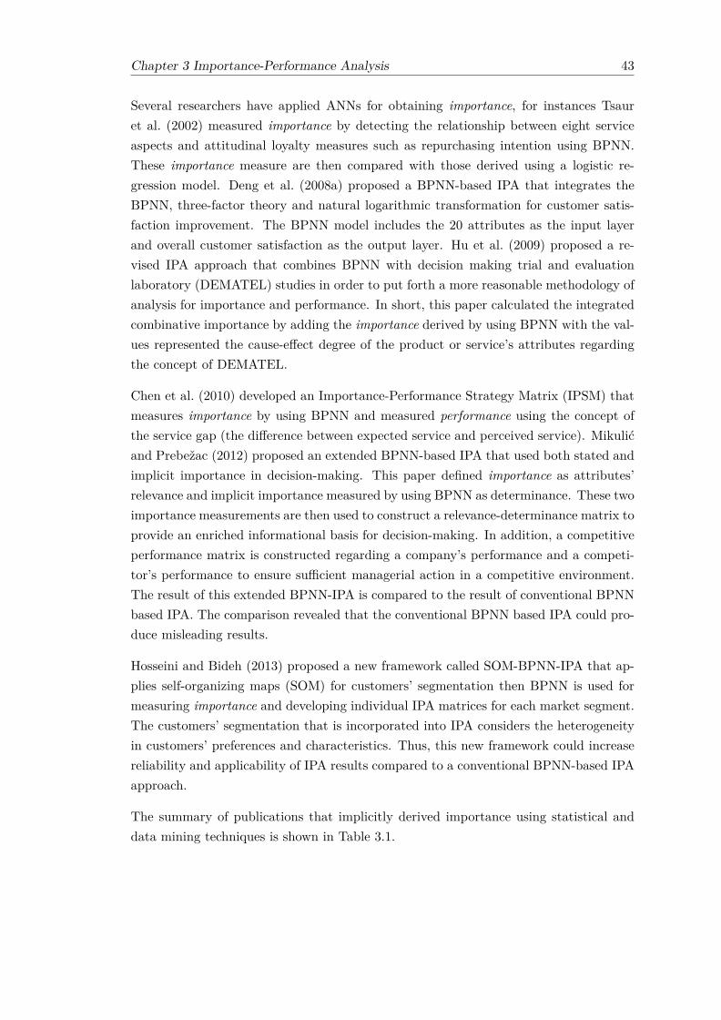
Chapter 3 Importance-Performance Analysis 43
Several researchers have applied ANNs for obtaining importance, for instances Tsauret al. (2002) measured importance by detecting the relationship between eight serviceaspects and attitudinal loyalty measures such as repurchasing intention using BPNN.These importance measure are then compared with those derived using a logistic re-gression model. Deng et al. (2008a) proposed a BPNN-based IPA that integrates theBPNN, three-factor theory and natural logarithmic transformation for customer satis-faction improvement. The BPNN model includes the 20 attributes as the input layerand overall customer satisfaction as the output layer. Hu et al. (2009) proposed a re-vised IPA approach that combines BPNN with decision making trial and evaluationlaboratory (DEMATEL) studies in order to put forth a more reasonable methodology ofanalysis for importance and performance. In short, this paper calculated the integratedcombinative importance by adding the importance derived by using BPNN with the val-ues represented the cause-effect degree of the product or service’s attributes regardingthe concept of DEMATEL.
Chen et al. (2010) developed an Importance-Performance Strategy Matrix (IPSM) thatmeasures importance by using BPNN and measured performance using the concept ofthe service gap (the difference between expected service and perceived service). Mikulićand Prebežac (2012) proposed an extended BPNN-based IPA that used both stated andimplicit importance in decision-making. This paper defined importance as attributes’relevance and implicit importance measured by using BPNN as determinance. These twoimportance measurements are then used to construct a relevance-determinance matrix toprovide an enriched informational basis for decision-making. In addition, a competitiveperformance matrix is constructed regarding a company’s performance and a competi-tor’s performance to ensure sufficient managerial action in a competitive environment.The result of this extended BPNN-IPA is compared to the result of conventional BPNNbased IPA. The comparison revealed that the conventional BPNN based IPA could pro-duce misleading results.
Hosseini and Bideh (2013) proposed a new framework called SOM-BPNN-IPA that ap-plies self-organizing maps (SOM) for customers’ segmentation then BPNN is used formeasuring importance and developing individual IPA matrices for each market segment.The customers’ segmentation that is incorporated into IPA considers the heterogeneityin customers’ preferences and characteristics. Thus, this new framework could increasereliability and applicability of IPA results compared to a conventional BPNN-based IPAapproach.
The summary of publications that implicitly derived importance using statistical anddata mining techniques is shown in Table 3.1.

44 Chapter 3 Importance-Performance Analysis
Table3.1:
Publicationsthat
implicitly
derivedim
portance
Citation(s)
Method
form
easuringM
ethodfor
measuring
Rem
arkim
portanceperform
anceMatzler
etal.(2003)
partialcorrelationanalysis
Actualperform
ance(rating
scale)-
Deng
etal.(2008b)
partialcorrelationanalysis
Relative
performance
(performance
ratio)-
Banand
Bogdan(2013)
partialcorrelationanalysis
Actualperform
ance(rating
scale)Using
thealternative
partitionsofthe
IPAgrid
Pezeshkietal.(2009)
MLR
Actualperform
ance(rating
scale)-
Hoet
al.(2012)the
combination
ofMLR
andDEM
ATEL
Actualperform
ance(rating
scale)-
Deng
etal.(2008a)
BPNN
Actualperform
ance(rating
scale)-
Huet
al.(2009)thecom
binationofBPN
Nand
DEM
ATEL
Actualperform
ance(rating
scale)-
Chen
etal.(2010)
BPNN
Actual
performance
(Servicegap)
gainedfrom
expectedperform
anceand
perceivedperform
ance
-
Mikulić
andPrebežac
(2012)stated
andim
plicitim
por-tance
usingBPN
NActual
andrelative
performance
(Gap
analysis)Provide
2matrices:
(1)Relevance-
determinance
matrix
and(2)
Com
pet-itive
performance
matrix
Hosseiniand
Bideh(2013)
BPNN
Actualperform
ance(rating
scale)Provide
individualIPA
sfor
eachcus-
tomer
segment
clusteredby
SOM

Chapter 3 Importance-Performance Analysis 45
3.2 Previous comparative studies of methods for measur-ing importance
Although the issue of implicitly derived versus self-stated importance has been debatedfor a period of time, as well as an increase in several methods used for measuringimportance, there were a few empirical studies that compared the different methodsagainst a set of evaluation criteria (Azzopardi and Nash, 2013). The summary of previouscomparative studies is shown in Table 3.2 and their detail is explained in the followingparagraphs.
Four previous empirical studies compared implicitly derived to self-stated importancemeasures. One of the first empirical studies was reported by Hauser (1991). Hauser com-pared three self-stated importance measures (including direct-rating scales, anchoredscales and constant-sum scales) to one statistically derived importance measures usinglinear regression. These methods were compared on the basis of predictive validity (abil-ity to predict actual overall customer satisfaction), relative predictive validity (abilityto predict customer-reported priority), and face validity. The result of Hauser (1991)supported the use of stated importance measures since all three stated importance mea-sures correlated highly with customer preference rank-order and had high face validityrelative to that of the regression-based importance measure.
Consistent with the finding of Hauser (1991), the second study by Bacon (2003) reportedthat self-stated importance measures using direct-rating scales performed better thancorrelation-based and regression-based importance measures since, the relative predictivevalidity estimated as the mean of adjusted R-squared of direct-rating scales across 15datasets was higher than that of correlation and regression. Although the self-statedimportance measure was superior to the two statistically derived importance measures,its adjusted R-squared of half datasets was considered fairly low which suggested thatit was a poor predictor of consumer priorities in those datasets.
The third empirical study by Gustafsson and Johnson (2004) reported the comparison ofimplicitly derived with self-stated importance measures on three datasets. Gustafssonand Johnson (2004) compared five statistically derived importance measures (includ-ing linear regression, normalized pairwise estimation, reflective/formative partial leastsquares, and principal components regression) to one self-stated importance measureusing direct-rating scales. These importance measures were compared against threeevaluation metrics which are predictive validity, diagnosticity (the ability to identifythe consumers’ most important attributes) and incidence of negative measures. Resultsshowed that there is no clear winner among statistically derived importance measures.Each method of deriving importance has its own advantages and limitations. On thecomparison of self-stated and implicitly derived importance measures, the results showed

46 Chapter 3 Importance-Performance Analysis
that the former reflected better attribute importance than the latter with respect to in-cidence of negative measures as the scale values are usually positive. The latter however,reflected better attribute importance than the former regarding both predictive validityand diagnosticity.
The fourth study by Taplin (2012b) provided additional evidence that self-stated relativeimportance was better than statistically derived importance measures using regression.Taplin (2012b) compared several models of absolute and relative self-stated importancewith regression-based importance measures and the models using both methods withthe predictive validity. The comparison of models using a single method showed thata regression-based importance measure yielded the highest predictive validity closelyfollowed by the self-stated relative importance measure interpreted on the power scale(denoted as SumRPpow).
However, Taplin (2012b) suggested that regression gained an advantage of predicting onthe same data from which it was calculated. Hence, a further test on Mean Squared Error(MSE) under a fair comparison using leave-one-out cross-validation was conducted andresults showed that SumRPpow provided higher predictive accuracy than regression-based importance measure. This led to the conclusion to support the use of self-statedrelative importance measures. Additionally, Taplin (2012b) reported that the impor-tance measure based on both self-stated relative importance and statistically derivedimportance produced the highest predictive validity.
In contrast to the first four studies, some researchers concentrated solely on comparingeither self-stated importance measures or implicitly derived importance measures. Cohen(2003) compared three self-stated importance measures including direct-rating scales,paired comparisons and Maximum Difference scaling (MaxDiff), and found that MaxDiffwas superior to direct-rating scales and slightly superior to paired comparisons regardingto relative predictive validity and discriminating power (ability to provide discriminatingmeasures).
In a similar vein, Chrzan and Golovashkina (2006) extended the previous comparativestudy by Cohen (2003) to add four more self-stated importance measures (includingmagnitude estimation, unbounded ratings, constant sum, and Q-sort) to compare withdirect-rating scales and MaxDiff. These six self-stated importance measures were com-pared against three evaluation metrics which are task length (average time to completetask), discriminating power and predictive validity. The comparative results showedthat MaxDiff has the highest predictive validity and greatest discriminating power inexchange for longest task length. Q-sort was the second highest ranked method as itspredictive validity was very nearly as good as MaxDiff and its discriminating powerwas also ranked after MaxDiff. Q-sort also had the advantage of taking less time tocomplete than MaxDiff and other methods except direct-rating scales. The two lowest

Chapter 3 Importance-Performance Analysis 47
ranked self-stated importance methods were unbound rating and direct-rating scalessince both methods had fairly low predictive validity and discriminating power.
A recent empirical study by Pokryshevskaya and Antipov (2014) focused on comparingnine statistical methods for deriving importance (including Pearson correlation, Kendallcorrelation, Spearman correlation, linear regression, partial least squares, multilayerperceptron, Shapley value decomposition, first-round effect, and Fields decomposition).These nine statistical methods for deriving importance were compared on the basis ofdiagnosticity (modified from (Gustafsson and Johnson, 2004)) and stability (a robustnessof importance estimation to a small change of data). The comparison based on two real-world datasets showed that none of the methods appeared to be the best regardingboth metrics simultaneously. Considering the average rank of methods according todiagnosticity and stability, the top three highest ranked methods were partial leastsquares, Shapley Value and Spearman correlation.
To recommend the best used method, Pokryshevskaya and Antipov (2014) carriedout further analysis using Monte-Carlo iterations to vary weights of the two metricsfrom 0.4 to 0.6 and observed the percentage of being ranked in the top three for eachmethod. Shapley value yielded the highest percentage among the methods therebyPokryshevskaya and Antipov (2014) supported the use of Shapley value as a method forderiving importance.
Regarding the summary of previous comparative studies presented in Table 3.2, a num-ber of times that each evaluation was used in the past comparative studies is shownin Table 3.3. Based on this table, evaluation metrics with the total number of stud-ies greater than or equal to 2 were identified as the common evaluation metrics whichwere further observed in order to form the set of evaluation metrics of this study. Ac-cordingly, 5 out of 8 evaluation metrics namely predictive validity, relative predictivevalidity, diagnosticity, an incidence of negative measures, and discriminative power wereobserved to decide whether or not they are suitable evaluation metrics in the context ofthe comparative study conducted in this thesis.
Consider the context of the comparative study of this thesis, two evaluation metricsnamely relative predictive validity and incidence of negative measures were excludedfrom the set of evaluation metrics. The remaining was formed as the set of evaluationmetrics of this study and their detail is provided in Section 5.2. The relative predic-tive validity was excluded from the set of evaluation metrics since the measurement ofthis metrics required the customer preference rank-order which is not contained in thedatasets used in the comparative study of this thesis. The incidence of negative measureswas excluded from the set of evaluation metrics since considering this metric providean unfair comparison between regression-based techniques (such as MLR, OLR) thatprone to produce negative measures with other techniques (such as direct-rating scales,BPNN, Naïve Bayes and BNs) that constantly produce positive measures.
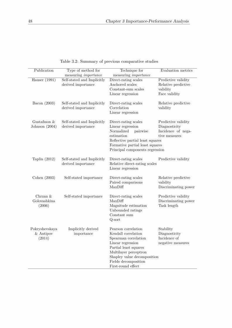
48 Chapter 3 Importance-Performance Analysis
Table 3.2: Summary of previous comparative studies
Publication Type of method for Technique for Evaluation metricsmeasuring importance measuring importance
Hauser (1991) Self-stated and Implicitly Direct-rating scales Predictive validityderived importance Anchored scales Relative predictive
Constant-sum scales validityLinear regression Face validity
Bacon (2003) Self-stated and Implicitly Direct-rating scales Relative predictivederived importance Correlation validity
Linear regression
Gustafsson & Self-stated and Implicitly Direct-rating scales Predictive validityJohnson (2004) derived importance Linear regression Diagnosticity
Normalized pairwiseestimation
Incidence of nega-tive measures
Reflective partial least squaresFormative partial least squaresPrincipal components regression
Taplin (2012) Self-stated and Implicitly Direct-rating scales Predictive validityderived importance Relative direct-rating scales
Linear regression
Cohen (2003) Self-stated importance Direct-rating scales Relative predictivePaired comparisons validityMaxDiff Discriminating power
Chrzan & Self-stated importance Direct-rating scales Predictive validityGolovashkina MaxDiff Discriminating power
(2006) Magnitude estimation Task lengthUnbounded ratingsConstant sumQ-sort
Pokryshevskaya Implicitly derived Pearson correlation Stability& Antipov importance Kendall correlation Diagnosticity(2014) Spearman correlation Incidence of
Linear regression negative measuresPartial least squaresMultilayer perceptronShapley value decompositionFields decompositionFirst-round effect

Chapter 3 Importance-Performance Analysis 49
Table 3.3: Evaluation metrics and their number of times used in the past com-parative studies
Evaluation metrics Description Total numberof studies
Predictive validity an ability to predict actual overall customer sat-isfaction
4
Relative predictivevalidity
an ability to predict customer-reported priority 3
Diagnosticity an ability to identify the consumers’ most impor-tant attributes
2
Incidence of nega-tive measures
a number of the negative coefficients for theregression-based method
2
Discriminatingpower
an ability to provide discriminating measures 2
Face validity a subjective assessment of whether or not thetechnique can measure importance
1
Task length an average time to complete task 1
Stability a robustness of importance estimation to a smallchange of data
1
3.3 Methodology for deriving importance
In this section, methods for deriving implicit importance by using statistical and datamining techniques such as MLR, BPNN, Naïve Bayes and BNs are described. The firsttwo techniques have been used to derive the importance from the survey data (Denget al., 2008a; Pezeshki et al., 2009; Ho et al., 2012; Mikulić and Prebežac, 2012) whilethe last two techniques have never before been applied to derive the importance.
The main tasks for deriving importance are exploring the relationship between the per-formance rating of each attribute of company’s product or service and the overall sat-isfaction, and estimating an impact of each attribute that has an effect on the overallcustomer satisfaction. A set of steps for deriving importance of each data mining tech-nique are described in the following sub-sections.
3.3.1 Method for deriving importance based on MLR
Since MLR is an easy-to-use technique, the procedure for deriving importance based onMLR is simple and straightforward. First, the performance rating of each attribute andthe overall satisfaction are defined as the independent and dependent variables respec-tively. Next, the regression model is trained and produces the regression coefficients.

50 Chapter 3 Importance-Performance Analysis
MLR model is easy to interpret by considering the signs and magnitude of coefficients.The sign of coefficient represents the existence of negative or positive effects of theindependent variables on the dependent variable. The magnitude of coefficient gener-ally indicates how much a one unit increase in the independent variable results in achange of the dependent variable with all other variables held constant (Nathans et al.,2012). Therefore, the regression coefficients can be referred to as implicit importancewhich express the influence of attributes of company’s product or service on the overallsatisfaction.
3.3.2 Method for deriving importance based on OLR
Similar to MLR, the procedure for deriving importance based on OLR is simple andstraightforward. First, the ordinal logistic model is build by specifying the performancerating of each attribute and the overall satisfaction are defined as the independent anddependent variables respectively. Additionally, the link function that would be the bestfit to the data set is chosen. Two major link functions commonly used in the OLR modelare logit and cloglog links(Chen and Hughes, 2004). Next, the regression coefficients areobtained from the trained model.
The coefficients obtained from the OLR model can also be referred to as implicit im-portance as with other types of regression. Specifically, the coefficient indicates that aone unit change on independent variable result in a change of the odds of dependentvariable, holding other independent variables as constant(Chen and Hughes, 2004).
3.3.3 Method for deriving importance based on BPNN
In contrast to the result of MLR which can be referred to as implicit importance, theresult of BPNN cannot be used directly as the importance hence there are two stepsfor deriving importance by using BPNN. The first step is the construction of a BPNNmodel in order to discover attributes of a company’s product or service that has themajor influence on overall satisfaction and selecting the model that produces the bestperformance. The second step is the computing of importance from the weights of theneural network. The contribution of each input to the outputs can be estimated throughthe connection weights since they are the links between the inputs and outputs. Themagnitude of connection weights indicates the effect of each input on the predictiveoutputs where the input with a larger connection weight has more contributions to theoutput, and therefore is more important than the input with a smaller one (Olden andJackson, 2002).
Step 1: Construct the BPNN prediction model for overall satisfactionThe BPNN model is modelled as one input layer, one hidden layer, and one output
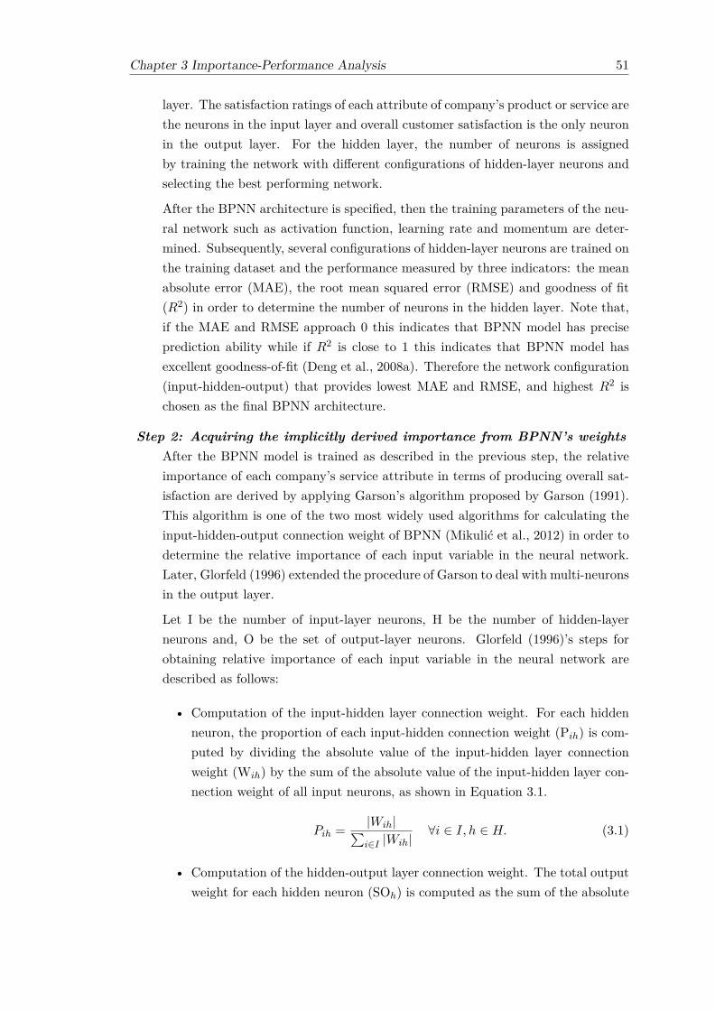
Chapter 3 Importance-Performance Analysis 51
layer. The satisfaction ratings of each attribute of company’s product or service arethe neurons in the input layer and overall customer satisfaction is the only neuronin the output layer. For the hidden layer, the number of neurons is assignedby training the network with different configurations of hidden-layer neurons andselecting the best performing network.
After the BPNN architecture is specified, then the training parameters of the neu-ral network such as activation function, learning rate and momentum are deter-mined. Subsequently, several configurations of hidden-layer neurons are trained onthe training dataset and the performance measured by three indicators: the meanabsolute error (MAE), the root mean squared error (RMSE) and goodness of fit(R2) in order to determine the number of neurons in the hidden layer. Note that,if the MAE and RMSE approach 0 this indicates that BPNN model has preciseprediction ability while if R2 is close to 1 this indicates that BPNN model hasexcellent goodness-of-fit (Deng et al., 2008a). Therefore the network configuration(input-hidden-output) that provides lowest MAE and RMSE, and highest R2 ischosen as the final BPNN architecture.
Step 2: Acquiring the implicitly derived importance from BPNN’s weightsAfter the BPNN model is trained as described in the previous step, the relativeimportance of each company’s service attribute in terms of producing overall sat-isfaction are derived by applying Garson’s algorithm proposed by Garson (1991).This algorithm is one of the two most widely used algorithms for calculating theinput-hidden-output connection weight of BPNN (Mikulić et al., 2012) in order todetermine the relative importance of each input variable in the neural network.Later, Glorfeld (1996) extended the procedure of Garson to deal with multi-neuronsin the output layer.
Let I be the number of input-layer neurons, H be the number of hidden-layerneurons and, O be the set of output-layer neurons. Glorfeld (1996)’s steps forobtaining relative importance of each input variable in the neural network aredescribed as follows:
• Computation of the input-hidden layer connection weight. For each hiddenneuron, the proportion of each input-hidden connection weight (Pih) is com-puted by dividing the absolute value of the input-hidden layer connectionweight (Wih) by the sum of the absolute value of the input-hidden layer con-nection weight of all input neurons, as shown in Equation 3.1.
Pih =|Wih|∑i∈I |Wih|
∀i ∈ I, h ∈ H. (3.1)
• Computation of the hidden-output layer connection weight. The total outputweight for each hidden neuron (SOh) is computed as the sum of the absolute

52 Chapter 3 Importance-Performance Analysis
value of the hidden-output layer connection weight (Woh) of all output neu-rons, as shown in Equation 3.2.
SOh =∑o∈O
|Woh| ∀h ∈ H. (3.2)
• Computation of input-hidden-output connection weight. The contributionof each neuron to the output via each hidden neuron (Cih) is computed bymultiplying the proportion of each input-hidden connection weight (Pih) pro-duced from Equation 3.1 by total output weight of the corresponding hiddenneuron (SOh) produced from Equation 3.2. The equation is shown below.
Cih = Pih × SOh ∀i ∈ I, h ∈ H. (3.3)
• Computation of the contribution for each input variable. For each inputvariable, the contribution (Si) is computed as the sum of the contribution ofeach neuron (Cih) produced from Equation 3.3 across all hidden neurons, asshown in Equation 3.4.
Si =∑h∈H
Cih ∀i ∈ I. (3.4)
• Computation of relative importance for each input variable. After the sum ofeach input neurons contribution is computed, the relative importance (RIi) iscalculated following to the Equation 3.5. This equation formats the relativeimportance as a percentage (%) as the ratio of Si to the overall contributionof all input neurons.
RIi =Si∑i∈I Si
× 100 ∀i ∈ I. (3.5)
In summary a method for deriving importance based on BPNN is the assessments ofcompany’ s service attributes are specified as input neurons and the overall satisfactionis specified as output neurons. BPNN with one hidden layer are trained and tested toestablish the relationship between these service aspects and the overall satisfaction. Inaddition, a number of neurons in the hidden layer is assigned by experimental trial. Afterthe BPNN model is trained, the importance can be calculated based on the extendedGarson’s algorithm proposed by Glorfeld (1996).
3.3.4 Method for deriving importance based on Naïve Bayes
There are two steps for conducting Naïve Bayes based IPA. The first step is the construc-tion of a Naïve Bayes model in order to discover the attributes of company’s product or
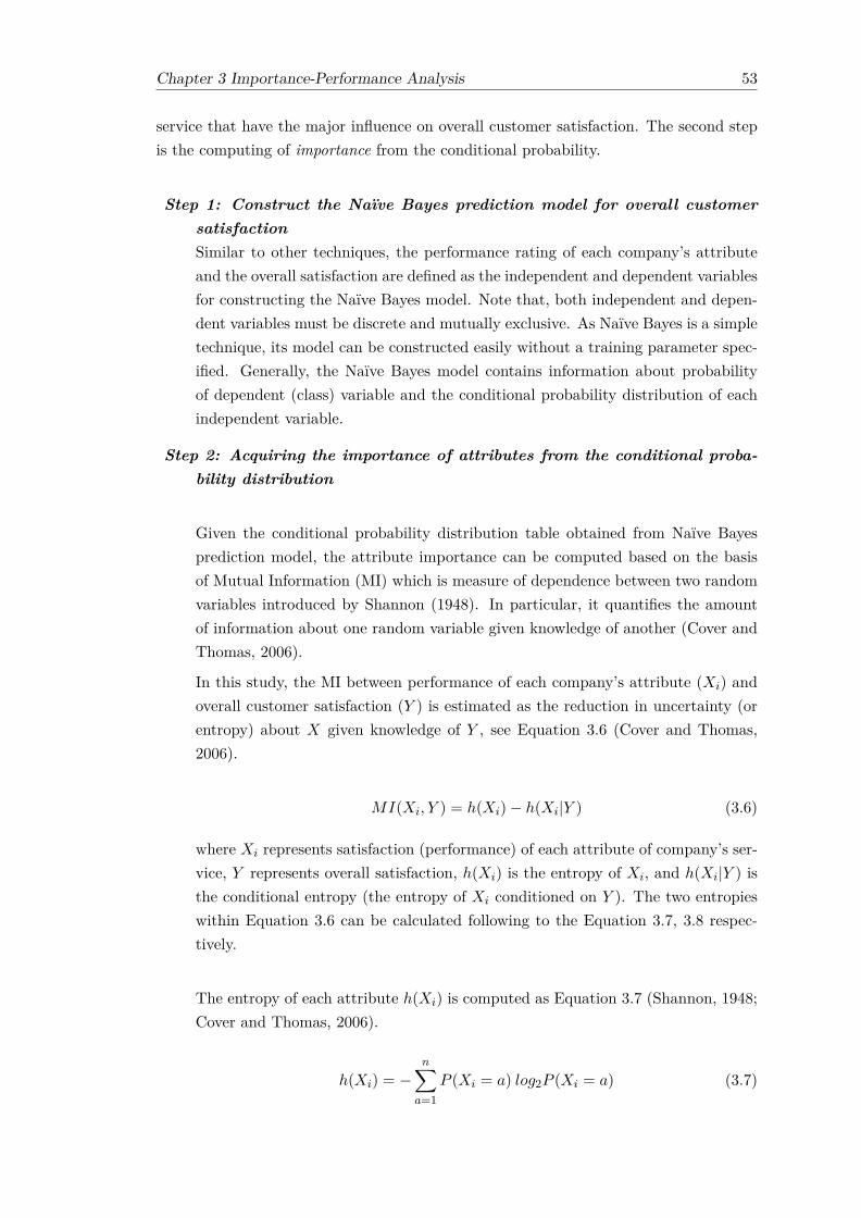
Chapter 3 Importance-Performance Analysis 53
service that have the major influence on overall customer satisfaction. The second stepis the computing of importance from the conditional probability.
Step 1: Construct the Naïve Bayes prediction model for overall customersatisfactionSimilar to other techniques, the performance rating of each company’s attributeand the overall satisfaction are defined as the independent and dependent variablesfor constructing the Naïve Bayes model. Note that, both independent and depen-dent variables must be discrete and mutually exclusive. As Naïve Bayes is a simpletechnique, its model can be constructed easily without a training parameter spec-ified. Generally, the Naïve Bayes model contains information about probabilityof dependent (class) variable and the conditional probability distribution of eachindependent variable.
Step 2: Acquiring the importance of attributes from the conditional proba-bility distribution
Given the conditional probability distribution table obtained from Naïve Bayesprediction model, the attribute importance can be computed based on the basisof Mutual Information (MI) which is measure of dependence between two randomvariables introduced by Shannon (1948). In particular, it quantifies the amountof information about one random variable given knowledge of another (Cover andThomas, 2006).
In this study, the MI between performance of each company’s attribute (Xi) andoverall customer satisfaction (Y ) is estimated as the reduction in uncertainty (orentropy) about X given knowledge of Y , see Equation 3.6 (Cover and Thomas,2006).
MI(Xi, Y ) = h(Xi)− h(Xi|Y ) (3.6)
where Xi represents satisfaction (performance) of each attribute of company’s ser-vice, Y represents overall satisfaction, h(Xi) is the entropy of Xi, and h(Xi|Y ) isthe conditional entropy (the entropy of Xi conditioned on Y ). The two entropieswithin Equation 3.6 can be calculated following to the Equation 3.7, 3.8 respec-tively.
The entropy of each attribute h(Xi) is computed as Equation 3.7 (Shannon, 1948;Cover and Thomas, 2006).
h(Xi) = −n∑
a=1
P (Xi = a) log2P (Xi = a) (3.7)
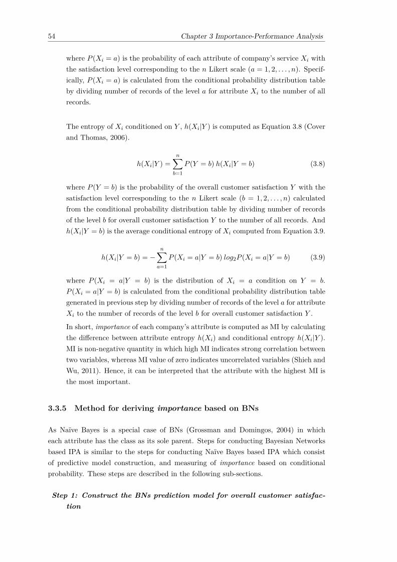
54 Chapter 3 Importance-Performance Analysis
where P (Xi = a) is the probability of each attribute of company’s service Xi withthe satisfaction level corresponding to the n Likert scale (a = 1, 2, . . . , n). Specif-ically, P (Xi = a) is calculated from the conditional probability distribution tableby dividing number of records of the level a for attribute Xi to the number of allrecords.
The entropy of Xi conditioned on Y , h(Xi|Y ) is computed as Equation 3.8 (Coverand Thomas, 2006).
h(Xi|Y ) =
n∑b=1
P (Y = b) h(Xi|Y = b) (3.8)
where P (Y = b) is the probability of the overall customer satisfaction Y with thesatisfaction level corresponding to the n Likert scale (b = 1, 2, . . . , n) calculatedfrom the conditional probability distribution table by dividing number of recordsof the level b for overall customer satisfaction Y to the number of all records. Andh(Xi|Y = b) is the average conditional entropy of Xi computed from Equation 3.9.
h(Xi|Y = b) = −n∑
a=1
P (Xi = a|Y = b) log2P (Xi = a|Y = b) (3.9)
where P (Xi = a|Y = b) is the distribution of Xi = a condition on Y = b.P (Xi = a|Y = b) is calculated from the conditional probability distribution tablegenerated in previous step by dividing number of records of the level a for attributeXi to the number of records of the level b for overall customer satisfaction Y .
In short, importance of each company’s attribute is computed as MI by calculatingthe difference between attribute entropy h(Xi) and conditional entropy h(Xi|Y ).MI is non-negative quantity in which high MI indicates strong correlation betweentwo variables, whereas MI value of zero indicates uncorrelated variables (Shieh andWu, 2011). Hence, it can be interpreted that the attribute with the highest MI isthe most important.
3.3.5 Method for deriving importance based on BNs
As Naïve Bayes is a special case of BNs (Grossman and Domingos, 2004) in whicheach attribute has the class as its sole parent. Steps for conducting Bayesian Networksbased IPA is similar to the steps for conducting Naïve Bayes based IPA which consistof predictive model construction, and measuring of importance based on conditionalprobability. These steps are described in the following sub-sections.
Step 1: Construct the BNs prediction model for overall customer satisfac-tion
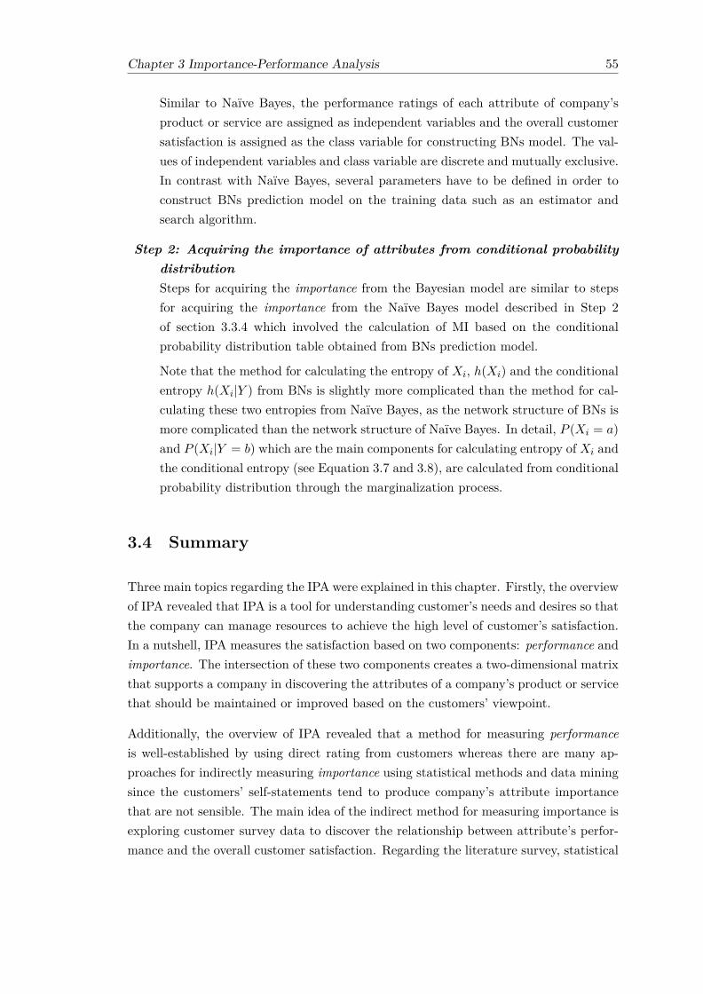
Chapter 3 Importance-Performance Analysis 55
Similar to Naïve Bayes, the performance ratings of each attribute of company’sproduct or service are assigned as independent variables and the overall customersatisfaction is assigned as the class variable for constructing BNs model. The val-ues of independent variables and class variable are discrete and mutually exclusive.In contrast with Naïve Bayes, several parameters have to be defined in order toconstruct BNs prediction model on the training data such as an estimator andsearch algorithm.
Step 2: Acquiring the importance of attributes from conditional probabilitydistributionSteps for acquiring the importance from the Bayesian model are similar to stepsfor acquiring the importance from the Naïve Bayes model described in Step 2of section 3.3.4 which involved the calculation of MI based on the conditionalprobability distribution table obtained from BNs prediction model.
Note that the method for calculating the entropy of Xi, h(Xi) and the conditionalentropy h(Xi|Y ) from BNs is slightly more complicated than the method for cal-culating these two entropies from Naïve Bayes, as the network structure of BNs ismore complicated than the network structure of Naïve Bayes. In detail, P (Xi = a)
and P (Xi|Y = b) which are the main components for calculating entropy of Xi andthe conditional entropy (see Equation 3.7 and 3.8), are calculated from conditionalprobability distribution through the marginalization process.
3.4 Summary
Three main topics regarding the IPA were explained in this chapter. Firstly, the overviewof IPA revealed that IPA is a tool for understanding customer’s needs and desires so thatthe company can manage resources to achieve the high level of customer’s satisfaction.In a nutshell, IPA measures the satisfaction based on two components: performance andimportance. The intersection of these two components creates a two-dimensional matrixthat supports a company in discovering the attributes of a company’s product or servicethat should be maintained or improved based on the customers’ viewpoint.
Additionally, the overview of IPA revealed that a method for measuring performanceis well-established by using direct rating from customers whereas there are many ap-proaches for indirectly measuring importance using statistical methods and data miningsince the customers’ self-statements tend to produce company’s attribute importancethat are not sensible. The main idea of the indirect method for measuring importance isexploring customer survey data to discover the relationship between attribute’s perfor-mance and the overall customer satisfaction. Regarding the literature survey, statistical

56 Chapter 3 Importance-Performance Analysis
methods that have been used for measuring importance are MLR, OLR, SEMs and par-tial correlation and BPNN, which is a predictive data mining technique, have recentlybecome an alternative approach for determining a company’s attribute importance.
Secondly, the past comparative studies of methods for measuring importance showed thatthere were a few empirical studies that compared the different methods against a set ofevaluation criteria. And the results of the past comparative studies were not along thesame lines, some studies supported the use of self-stated importance while some studiessupported the use of implicitly derived importance. The review of the past comparativestudies of methods for measuring importance also provided a background related to theevaluation metrics for setting-up the comparative experiment in Chapter 5.
Thirdly, methodologies for deriving importance were described to illustrate how theimportance can be derived from results of two statistical techniques- MLR, OLR andthree data mining techniques namely - BPNN, Naïve Bayes and BNs. MLR, OLRand BPNN have been used to derive the importance from the survey data while NaïveBayes and BNs have never before been applied to derive the importance. For eachtechnique, the main tasks for deriving importance are constructing the predictive modelthat discovers the relationship between the performance rating of each attribute andthe overall customer satisfaction, and acquiring importance from an outcome of thepredictive model. Specifically, methods for acquiring importance from an outcome ofeach technique are different since each technique produces a different form of outcome,for example; MLR and OLR produce regression coefficients, BPNN produces neuralnetwork weights, Naïve Bayes and BNs produce a conditional probability table.
Different importance measurement techniques will likely result in different IPA matrices.Therefore, the technique for measuring importance has to be carefully justified whichleads to the empirical experiment set up in Chapter 5. Additionally, research processand research methodology that were conducted to complete this study are explained inthe next chapter.

Chapter 4
Research Design
In the preceding chapters, the research goal and research questions as well as backgroundknowledge of this thesis were described. Before proceeding to the chapter that presentsthe research findings, it is important to describe a procedural plan for how this researchstudy is to be completed. Such a procedural plan is known as a research design anda well-defined research design is essential in providing valid research findings (Kumar,2011).
Thus, the main function of this chapter is explaining a procedural plan which consistsof the main tasks to be conducted throughout this study, and research methods to beused corresponding to each task. Section 4.1 provides an overview of the research designof this study. Section 4.2 - 4.5 provide detail for each phase of research design.
4.1 An overview of research design within this study
Among the three Information Technology (IT)-related disciplines which are InformationSystems (IS), Computer Science and Computer Systems Engineering (Avison and Elliot,2006), this research can be classified as IS research, an applied discipline, which empha-sises the applications of technology to address the range of operational, managerial andstrategic activities of organisations as this work applied knowledge in computer scienceto solve problems of organisations in conducting their business.
Consequently, the research work presented in this thesis was conducted based on adesign science research process in IS. According to Kuechler and Vaishnavi (2005), designscience research is a set of analytical techniques and perspectives for performing researchin IS. It involves the design and evaluation of novel or innovative artefacts in order tosolve observed problems of organisations (Hevner and Chatterjee, 2010).
57
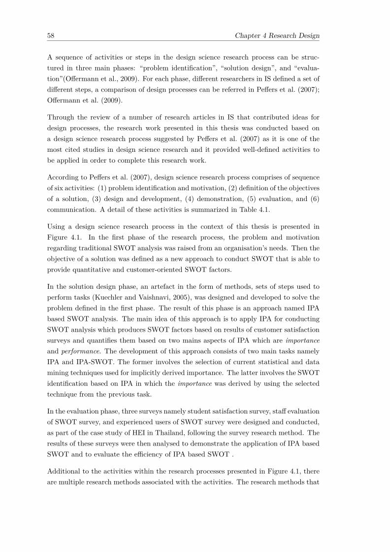
58 Chapter 4 Research Design
A sequence of activities or steps in the design science research process can be struc-tured in three main phases: “problem identification”, “solution design”, and “evalua-tion”(Offermann et al., 2009). For each phase, different researchers in IS defined a set ofdifferent steps, a comparison of design processes can be referred in Peffers et al. (2007);Offermann et al. (2009).
Through the review of a number of research articles in IS that contributed ideas fordesign processes, the research work presented in this thesis was conducted based ona design science research process suggested by Peffers et al. (2007) as it is one of themost cited studies in design science research and it provided well-defined activities tobe applied in order to complete this research work.
According to Peffers et al. (2007), design science research process comprises of sequenceof six activities: (1) problem identification and motivation, (2) definition of the objectivesof a solution, (3) design and development, (4) demonstration, (5) evaluation, and (6)communication. A detail of these activities is summarized in Table 4.1.
Using a design science research process in the context of this thesis is presented inFigure 4.1. In the first phase of the research process, the problem and motivationregarding traditional SWOT analysis was raised from an organisation’s needs. Then theobjective of a solution was defined as a new approach to conduct SWOT that is able toprovide quantitative and customer-oriented SWOT factors.
In the solution design phase, an artefact in the form of methods, sets of steps used toperform tasks (Kuechler and Vaishnavi, 2005), was designed and developed to solve theproblem defined in the first phase. The result of this phase is an approach named IPAbased SWOT analysis. The main idea of this approach is to apply IPA for conductingSWOT analysis which produces SWOT factors based on results of customer satisfactionsurveys and quantifies them based on two mains aspects of IPA which are importanceand performance. The development of this approach consists of two main tasks namelyIPA and IPA-SWOT. The former involves the selection of current statistical and datamining techniques used for implicitly derived importance. The latter involves the SWOTidentification based on IPA in which the importance was derived by using the selectedtechnique from the previous task.
In the evaluation phase, three surveys namely student satisfaction survey, staff evaluationof SWOT survey, and experienced users of SWOT survey were designed and conducted,as part of the case study of HEI in Thailand, following the survey research method. Theresults of these surveys were then analysed to demonstrate the application of IPA basedSWOT and to evaluate the efficiency of IPA based SWOT .
Additional to the activities within the research processes presented in Figure 4.1, thereare multiple research methods associated with the activities. The research methods that
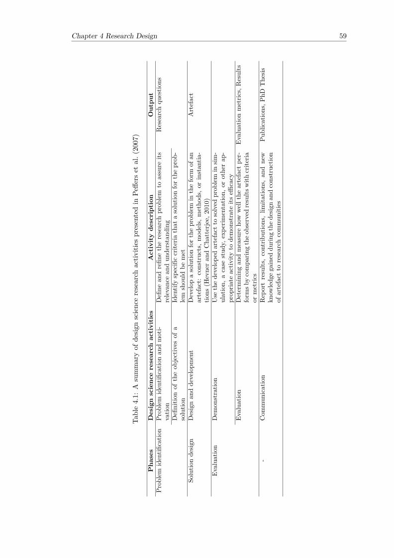
Chapter 4 Research Design 59
Table4.1:
Asummaryof
desig
nscienceresearch
activ
ities
presentedin
Peffe
rset
al.(
2007
)
Pha
ses
Designscienc
eresearch
activities
Activityde
scription
Outpu
tPr
oblem
identifi
catio
nPr
oblem
identifi
catio
nan
dmoti-
vatio
nDefi
nean
drefin
etheresearch
prob
lem
toassure
itsrelevanc
ean
dun
derstand
ing
Researchqu
estio
ns
Defi
nitio
nof
theob
jectives
ofa
solutio
nIdentifyspecificcrite
riathat
asolutio
nfort
heprob
-lem
shou
ldbe
met
Solutio
nde
sign
Designan
dde
velopm
ent
Develop
asolutio
nfort
heprob
lem
intheform
ofan
artefact:construc
ts,m
odels,
metho
ds,o
rinstan
tia-
tions
(Hevne
ran
dCha
tterjee,
2010
)
Artefact
Evalua
tion
Dem
onstratio
nUse
thede
velope
dartefact
tosolved
prob
lem
insim
-ulation,
acase
stud
y,expe
rimentatio
n,or
othe
rap
-prop
riate
activ
ityto
demon
strate
itseffi
cacy
Evalua
tion
Determiningan
dmeasure
how
welltheartefact
per-
form
sbycompa
ringtheo
bservedresults
with
crite
riaor
metric
s
Evalua
tionmetric
s,Results
-Com
mun
ication
Rep
ortresults
,contrib
utions,lim
itatio
ns,an
dne
wkn
owledg
egaine
ddu
ringthed
esignan
dconstruc
tion
ofartefact
toresearch
commun
ities
Publications,P
hDThe
sis

60 Chapter 4 Research Design
Figure 4.1: Research design scenario
were used to perform these activities were selected from a study on the methodolo-gies applied in and accepted by seven leading MIS journals during 1993-2003 by Palviaet al. (2004). Specifically, the four selected research methods include library research,frameworks & conceptual models, survey and laboratory experiment. Their details areprovided in Table 4.2.
Table 4.2: MIS Methodologies retained for this research based on Palvia et al.(2004)
Method DefinitionLibrary research Research that is based mainly on review, summarize and syn-
thesize existing literature.
Frameworks & Research that intends to develop a framework or a conceptualconceptual models model
Survey Research that uses predefined and structured questions to cap-ture data from individuals
Laboratory experiment Research in a simulated laboratory environment that manipu-lates and controls the various experimental variables and sub-jects

Chapter 4 Research Design 61
Library research is the first point of departure for a research journey as it establishes theneed for the research. Library research also serves many important purposes related dif-ferent activities in research process (Offermann et al., 2009). For example, the activitiesin problem identification phase employed library research to identify a problem as well asgain insight and understand the identified problem. The activity in the solution designphase employed library research to provide information relating to a possible solution tosolve the problem. In this thesis, the library research was employed for accomplishingresearch activities in the first two phases.
According to Håkansson (2013), frameworks and conceptual models method is used fordeveloping new concepts or interpreting existing concepts that are built upon the resultof library research. In this thesis, conceptual research is represented in the form of themethodological framework for generating SWOT or artefact in the form of method inthe context of design science research process.
Survey research involves the selection of a representative sample from a well-definedpopulation and the use of data analysis techniques to generalize from that sample to thepopulation (Pinsonneault and Kraemer, 1993). Normally, data for the survey research iscollected from individuals by means of structured and predefined questions. The surveyresearch was the most widely used research methodology by researchers in MIS researchduring 1993-2003 (Palvia et al., 2004) and is still in predominant use.
The survey research strengths lay in its ability of obtaining information from a largesample of the population and its ability to elicit information about attitude that is dif-ficult to acquire using observational techniques (Glasow, 2005). The survey researchweaknesses lay in its subjective nature in which bias in respondents or researcher mayoccur, the lack of response from respondents, and intentional misreporting by respon-dents (Glasow, 2005). In this thesis, survey research was employed for the purpose ofevaluation of the method for generating SWOT.
Laboratory experiment involves examination of a phenomenon in a controlled setting.It is conducted to investigate how the variables in the study are related by manipulatingone or more independent variables and measuring their impact on one or more outcome(dependent) variables (Easterbrook et al., 2008). In the case of this thesis, laboratoryexperiment was carried out to investigate the link between the type of statistical anddata mining techniques and their performance on measuring importance. The degree ofchange in performance in different groups of techniques is then compared to identify thesuitable technique for measuring importance.
One or more research methods may be employed to perform each activity within theresearch process. The connection between the research process, research methods, re-search questions, and thesis chapters is shown in Table 4.3 and details of each phase inthe research process and related research methods are described in the following sub-sections.
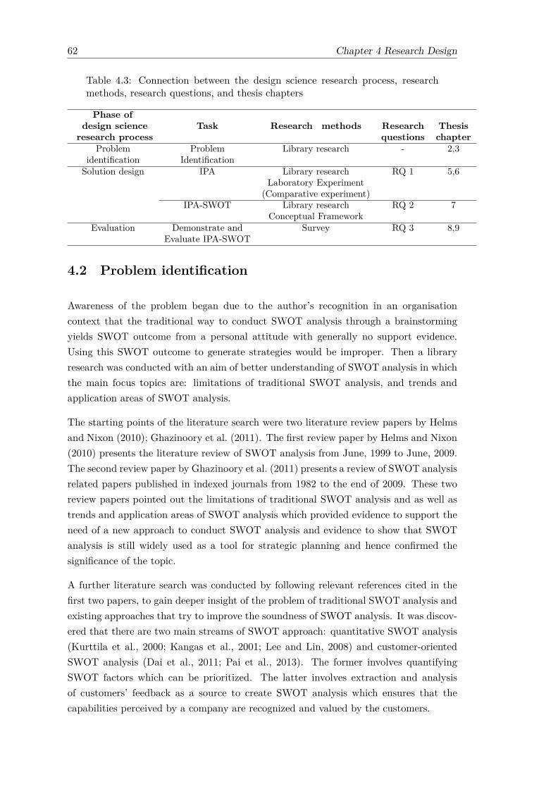
62 Chapter 4 Research Design
Table 4.3: Connection between the design science research process, researchmethods, research questions, and thesis chapters
Phase ofdesign science Task Research methods Research Thesis
research process questions chapterProblem Problem Library research - 2,3
identification IdentificationSolution design IPA Library research RQ 1 5,6
Laboratory Experiment(Comparative experiment)
IPA-SWOT Library research RQ 2 7Conceptual Framework
Evaluation Demonstrate and Survey RQ 3 8,9Evaluate IPA-SWOT
4.2 Problem identification
Awareness of the problem began due to the author’s recognition in an organisationcontext that the traditional way to conduct SWOT analysis through a brainstormingyields SWOT outcome from a personal attitude with generally no support evidence.Using this SWOT outcome to generate strategies would be improper. Then a libraryresearch was conducted with an aim of better understanding of SWOT analysis in whichthe main focus topics are: limitations of traditional SWOT analysis, and trends andapplication areas of SWOT analysis.
The starting points of the literature search were two literature review papers by Helmsand Nixon (2010); Ghazinoory et al. (2011). The first review paper by Helms and Nixon(2010) presents the literature review of SWOT analysis from June, 1999 to June, 2009.The second review paper by Ghazinoory et al. (2011) presents a review of SWOT analysisrelated papers published in indexed journals from 1982 to the end of 2009. These tworeview papers pointed out the limitations of traditional SWOT analysis and as well astrends and application areas of SWOT analysis which provided evidence to support theneed of a new approach to conduct SWOT analysis and evidence to show that SWOTanalysis is still widely used as a tool for strategic planning and hence confirmed thesignificance of the topic.
A further literature search was conducted by following relevant references cited in thefirst two papers, to gain deeper insight of the problem of traditional SWOT analysis andexisting approaches that try to improve the soundness of SWOT analysis. It was discov-ered that there are two main streams of SWOT approach: quantitative SWOT analysis(Kurttila et al., 2000; Kangas et al., 2001; Lee and Lin, 2008) and customer-orientedSWOT analysis (Dai et al., 2011; Pai et al., 2013). The former involves quantifyingSWOT factors which can be prioritized. The latter involves extraction and analysisof customers’ feedback as a source to create SWOT analysis which ensures that thecapabilities perceived by a company are recognized and valued by the customers.

Chapter 4 Research Design 63
The literature search through these two approaches revealed that each approach focuseson improving a different aspect of SWOT analysis. While the first approach can makeSWOT factors commensurable, these SWOT factors focus solely on a company’s per-spective and ignore the customer’s perspective. On the other hand, the second approachgenerates SWOT factors from a customer’s perspective but it has no means to prioritizeSWOT factors. This can be identified as a gap between the two current approaches ofSWOT analysis which will be filled by developing this research work. After the problemwas identified as previously stated, the objective of a solution to the problem was thendefined as a new approach to conduct SWOT that is able to provide quantitative andcustomer-oriented SWOT factors.
4.3 Solution design: IPA
Based on the results of the problem identification phase, a method was chosen as thedesign artefacts and customer satisfaction survey was chosen as a source of data forconducting SWOT analysis. Library research was also conducted in this phase to finda technique that can be employed to analyse customer satisfaction and develop SWOTanalysis based upon its result. For this purpose, several publications related to customersatisfaction analysis were retrieved by querying scientific search engines such as the IEEEExplore and ACM Digital Library, and then following relevant references cited in thediscovered papers. The review of these papers led to the decision of applying IPA todevelop a new approach of SWOT analysis.
Consequently, a further library research was conducted to review the state-of-the-artof IPA starting with highly cited papers such as Martilla and James (1977); Matzleret al. (2003); Bacon (2003) then the literature search was gradually fanned out to otherrelevant papers. Through this process, one technical issue of IPA regarding an indirectmethod for measuring importance (Lai and Hitchcock, 2015) was chosen to be studiedwithin this research work since, currently there are no well-established methods formeasuring importance (Gustafsson and Johnson, 2004; Fontenot et al., 2007; Feng et al.,2014).
Focusing on the issue of techniques for measuring indirect importance, the experimentwas set to compare three currently used indirect measurement techniques namely MLR,OLR, BPNN with the two new introduced techniques for measuring indirect importancenamely Naïve Bayes, and BNs. BNs was introduced for deriving importance since ithas been applied to analyse the customer satisfaction surveys (Salini and Kenett, 2009)which closely related to importance measure in IPA. Naïve Bayes was included in thecomparative experiment as it is a special case of BNs (Grossman and Domingos, 2004).
64 Chapter 4 Research Design
In addition to the indirect importance measurement techniques to be compared in theexperiment, the evaluation metrics used to decide the appropriate techniques for mea-suring importance were also defined through the review of previous comparative studiesi.e. Hauser (1991); Bacon (2003); Gustafsson and Johnson (2004). Specifically, the threeevaluation metrics were selected from eight evaluation metrics based on the number oftimes that it has been used in previous comparative studies.
Three datasets of customer satisfaction survey were used in this experiment. The firsttwo datasets were published datasets which have been used by other researchers (Kenettand Salini, 2012, p. 19) and (Azzalini et al., 2012). The third dataset was a studentsatisfaction survey collected from a leading Thai University for demonstrating the useof the design artefact.
To ensure that the comparative experiment were properly conducted, two baseline ex-periments were conducted before starting the comparative experiment. Further detailsregarding the baseline experiments and comparative experiment set up, and the experi-mental results are presented in Chapter 5 and Chapter 6 respectively.
4.4 Solution design: IPA-SWOT
Based on the result of solution design phase for IPA, a technique for measuring impor-tance was identified and applied in a methodological framework for developing SWOTanalysis from IPA results, called IPA based SWOT analysis.
Before starting to design the methodological framework, the library research was con-ducted to review the connection between IPA and SWOT analysis and specify the pos-sible way to acquire all SWOT aspects from the IPA results, known as IPA matrix.The review of literature indicated the correspondence between IPA and SWOT analysissince each quadrant of the IPA matrix can be interpreted as major/minor strength andweakness (Garver, 2003; Deng et al., 2008a; Silva and Fernandes, 2012; Hasoloan et al.,2012; Cugnata and Salini, 2013; Hosseini and Bideh, 2013).
Since, only strength and weakness can be inferred from the IPA matrix. Further libraryresearch was conducted to identify a possible solution to infer opportunity and threatfrom the IPA matrix which provided a complete aspect of SWOT analysis. This led toa decision to apply idea of Pai et al. (2013) to identify opportunity and threat based onthe IPA matrix of a company’s competitor as it is a sensible idea and can be practicallyapplied in the context of this research. At the end of this phase, the methodologicalframework to develop SWOT analysis from IPA was designed, the detail is discussed inChapter 7.

Chapter 4 Research Design 65
4.5 Evaluation through the survey research
After IPA based SWOT analysis was developed, it was executed in the context of aUniversity in Thailand to demonstrate and evaluate its efficacy. Three surveys weredeveloped for this purpose which are student satisfaction survey, staff evaluation ofSWOT survey, and experienced users of SWOT survey. The first survey was developedto collect student satisfaction and then used as the data source to implement the IPAbased SWOT analysis in a real-world context. The last two surveys were developed toevaluate the efficacy of IPA based SWOT analysis after implementing on data of thefirst survey, using quantitative measure since, currently there are no direct methods andtools for validating the effectiveness of SWOT analysis (Ayub et al., 2013).
Specifically, the staff evaluation of the IPA based SWOT analysis, was conducted usinga survey to collect the staff’s agreement on the analysis; to check whether the staff agreeor disagree with the resulting SWOT analysis. The experienced users of SWOT surveyinvolves the collection of MBA students’ rating on the quality of outcome of IPA basedSWOT analysis. In this section, the main aspects corresponding to the survey design areprovided for which further details including pilot study, sample size and ethic approvalrelated to each survey are provided in Chapter 8.
The main aspects of each survey including group of participant, survey media, andquestion type, contact method, and administration method are summarized in Table 4.4.And the detail of each aspect regarding possible methods that could have been used andthe justification for the selection of specific method is provided in the following sub-sections.
Table 4.4: Detail of three surveys used for demonstration and evaluation of IPAbased SWOT analysis
Student satisfaction Staff evaluation Experienced userssurvey of SWOT survey of SWOT survey
Purpose: Demonstration Evaluation Evaluation
Group of participant: Undergraduate University staff MBA studentsstudents
Survey Media: Written Survey Written Survey Written Survey
Survey Question type: Closed-ended Closed-ended Closed-ended andquestions questions open-ended questions
Contact method: Personal contact E-mail Personal contact(via class room) (via class room)
Administration Internet-mediated Internet-mediated Deliverymethod: and collection

66 Chapter 4 Research Design
4.5.1 Selecting survey media
Three types of survey media which are written survey, verbal survey and mixed modesurvey (Glasow, 2005) were investigated to choose one that fitted-well with the contextof this study. According to Glasow (2005), written survey is known as questionnaireand verbal survey is interview. Mixed mode survey is a combination of the written andverbal survey.
The written survey was chosen as the media to collect data for the three surveys for thereason that the data will be analysed by means of quantitative research using statisticaland data mining techniques. While the use of a verbal survey allows a researcher toget more qualitative data, in particular, it is difficult to summarize and incorporatestatistical analysis (Saunders et al., 2009).
Additionally, face-to-face interview is not applicable to use as a survey media of thisstudy since the responses to the student satisfaction survey need to be anonymous toavoid intentional misreporting by respondents so as to the response to the staff evaluationof SWOT survey. While the telephone interview can keep the response anonymous, ittakes time and cost to schedule and to establish a call for participants of this study.
4.5.2 Selecting survey questions
There are two types of survey questions: open-ended and closed-ended questions. Theformer allows respondents to formulate their own answers which enable the researcherto explore ideas of respondents while the latter forces respondents to choose an answerfrom a given set of responses (Glasow, 2005; Fink, 2012b).
Generally, the closed-ended questions require minimal thought and writing hence it isusually quicker and easier to answer than the open-ended questions which require greaterthought to respond, and therefore, take a longer time to answer (Saunders et al., 2009).The results obtained from open-ended questions are also more difficult to compare andanalyse (Glasow, 2005).
The closed-ended questions were used to collect quantitative data regarding student sat-isfaction as the specification of input data for IPA. Specifically, a survey that is suitablefor applying IPA contains assessment of respondents satisfaction for an organisation’sproduct or service measured by a Likert scale with either five or seven levels.
The closed-ended questions were also used to collect quantitative data of the second andthird survey as the main purpose for data collection of these two surveys was to providea quantitative measure to evaluate the IPA based SWOT analysis. In addition to theclosed-ended questions, one open-ended question was used to ask the respondents of thethird survey about their suggestion toward the IPA based SWOT analysis. This allowed

Chapter 4 Research Design 67
respondents of the third survey who had experienced in generating SWOT give someuseful ideas regarding IPA based SWOT analysis.
4.5.3 Selecting contact method
Possible ways to contact the respondents to take part in each survey of this study wereinvestigated. The three possible contact methods are postal/e-mail, telephone, andpersonal contact. By considering contact methods that are the most convenient wayto contact different group of respondents, e-mail and personal contact were chosen tocontact the respondents to take part in this study.
Respondents of the first and the third survey who are undergraduate and graduatestudents (see Table 4.4) respectively were asked face to face to take part in the surveyby the representative of the researcher at the end of their class. This guarantees that themajority of respondents were invited to take part in the survey which may increase theresponse rate, and allows the representative of the researcher to explain the objective ofthe survey.
To avoid the potential error that may occur during survey process since the researchercannot physically be present to contact respondents and administer the survey by herselfbecause of the limitation of place and time, the representative of the researcher hadbeen already informed about the procedure to administer the survey and discussed theobjective of the survey with the researcher prior to the survey administration.
Respondents of the second survey who are university staff including academic and non-academic staff were asked to take part in the survey by e-mail. This is a formal wayto contact university staff and an easy way to follow-up their response. Besides, usinge-mail is also convenient for respondents to answer when they are available.
Among the three possible contact methods, telephone was not chosen to be used althoughit is a quick method. This is because it involves a call cost and it is difficult to find phonenumber of all respondents especially with the large numbers of respondents. Besides, itis less formal to contact respondents who are university staff via telephone than e-mail.
4.5.4 Selecting administration method
The range of methods for collecting survey data can be classified into two major groupsaccording to how a survey is administered and these are self-administered and interviewer-administered method. The written survey is collected through the self-administeredmethod since the written survey is usually completed by respondents themselves whereasverbal survey is collected through the interviewer-administered method since it is usu-ally carried out by interviewer who asks and records answer of respondents (Saunderset al., 2009).
68 Chapter 4 Research Design
Since only written survey is used in this study, only the self-administered method isconsidered as a major type for administering survey. The self-administered method isdivided into three types: a delivery and collection, an internet-mediated, and postal/e-mail. Main aspects of each method are compared in Table 4.5.
Through the investigation of characteristics for each mode of data collection, postal/e-mail was not a choice of administering survey within this study for the reason that thismethod takes the longest data collection period and it is practically difficult to obtaine-mail or address of all respondents. Therefore, two self-administered methods whichare delivery and collection and internet-mediated were selected to be used in this study.
Specifically, data for the first and second survey were collected through online surveysdeveloped by using iSurvey, a free to use survey generation tool for members of theUniversity of Southampton. By using internet-mediated as the method of data col-lection, the anonymity of respondents can be assured and respondents can take theirtime to answer the questions on their own schedule. The anonymity and the time toconsider questions were important factors if respondents were to provide honest andaccurate data, and thereby improve the quality of responses (De Vaus, 2002a). Besides,respondents’ answers are automatically stored in an electronic file ready for analysis.
Data for the third survey were collected using a delivery and collection method wherebyeach questionnaire was delivered and collected in the classroom since the questionnaireof the third survey is more complicated than that of the first two surveys. Using thisdelivery and collection method allows respondents to ask for clarification during comple-tion from the survey administrator which reduces potential error such as uncompletedquestions that can affect the quality of responses.
4.6 Summary
This chapter explains the research process and research methodology that have beenused for completing this research study. By means of the design science research pro-cess, a sequence of the research process was divided into three main phases: “problemidentification”, “solution design”, and “evaluation”.
In the problem identification phase, the problem of this study was formulated as currentSWOT analysis approaches have no means to generate and prioritize SWOT factorsbased on customer’s perspective. This problem was first raised by the author’s recog-nition in an organisation context and then it was established through the literaturesearch.
In the solution design phase, a sets of step used to perform SWOT analysis that is able toprovide quantitative and customer-oriented SWOT factors, was designed and developedwhich is called IPA based SWOT analysis. The main idea of this approach is to apply
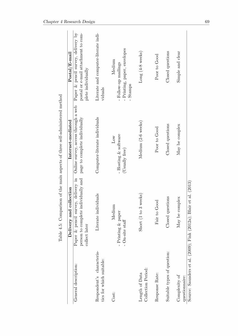
Chapter 4 Research Design 69
Table4.5:
Com
paris
onof
themainaspe
ctsof
threeself-ad
minist
ered
metho
d
Deliveryan
dcolle
ction
Internet-m
ediated
Postal/E-m
ail
General
descrip
tion:
Pape
r&
pencil
survey,deliv
eryin
person
tocompleteindividu
ally
and
colle
ctlater
Onlinesurvey,a
ccesst
hrou
ghawe
bpa
geto
completeindividu
ally
Pape
r&
pencilsurvey,deliv
eryby
postal
ore-maila
ttachm
entt
ocom-
pleteindividu
ally
Respo
ndent’s
characteris
-tic
sforwhich
suita
ble:
Literate
individu
als
Com
puter-literateindividu
als
Literate
andcompu
ter-literateindi-
vidu
als
Cost:
Medium
Low
Medium
-Prin
ting&
pape
r-H
ostin
g&
softw
are
-Follow-upmailin
gs-O
n-sit
estaff
(Usually
free)
-Prin
ting,
pape
r,envelope
s-S
tamps
Leng
thof
Data
Short(1
to3we
eks)
Medium
(2-6
weeks)
Long
(4-8
weeks)
CollectionPe
riod:
Respo
nseRate:
Fair
toGoo
dPo
orto
Goo
dPo
orto
Goo
d
Suita
bletype
sof
questio
n:Closedqu
estio
nsClosedqu
estio
nsClosedqu
estio
ns
Com
plexity
ofMay
becomplex
May
becomplex
Simplean
dclear
questio
nnaire:
Source:Sa
unders
etal.(
2009
);Fink
(2012a);
Blairet
al.(
2013
)

70 Chapter 4 Research Design
IPA for conducting SWOT analysis which produces SWOT factors based on results ofcustomer satisfaction survey and quantifies them based on two mains aspects of IPAwhich are importance and performance.
The development of the IPA based SWOT analysis consists of two main tasks namelyIPA and IPA-SWOT. The former involves the comparative experiment method for se-lection the current statistical and data mining techniques used for implicitly derivedimportance. Further details regarding the experiment set up and the experimental re-sults are presented in Chapter 5 and Chapter 6 respectively. The latter involves theconstruction of the IPA based SWOT analysis framework in other words it involves theidentification SWOT factors based on IPA in which the importance was derived by usingthe selected technique from the previous task. Further detail regarding the developmentof SWOT analysis from IPA is designed and presented in Chapter 7.
In the evaluation phase, three surveys were conducted for the purpose of demonstratingthe application of IPA based SWOT and to evaluate the efficiency of the approach.Through the review of methods related to the survey design, the written survey usingclosed-ended questions was selected as a survey media. Personal contact and e-mailwere used as a method to contact the respondents to take part in the survey. Theselection was made based on type of respondents which are students and universitystaff. After the respondents were contacted to take part in the survey, the first twosurveys were administered to the respondents using internet-mediated method while thethird survey was administered to the respondents using delivery and collection method.Further details of the survey design including pilot study, sample size and ethics approvalrelated to each survey can be seen in Chapter 8.

Chapter 5
Experiment: Empiricalcomparison of importancemeasuring techniques
It was suggested in Chapter 3 that currently there are no well-established importancemeasurement techniques and different importance measurement techniques are likely toresult in identifying dramatically different attributes for improvement. Such unsettledissue of IPA leads to the conducting of a comparative experiment described in thischapter.
The main function of this chapter is explaining how the comparative experiment is to beconducted in order to select a potential importance measurement technique to be used forSWOT analysis so as to answer the first research question “Which importance measureshould be used in IPA?” The techniques for measuring importance being investigatedare (1) Direct-rating scales (DR), (2) MLR, (3) OLR, (4) BPNN, (5) Naïve Bayes and(6) Bayesian Networks (BNs). The first four techniques have been used to measureimportance while the last two have never before been applied to derive importance fromthe survey data. Attribute importance measured by these techniques will be comparedagainst three evaluation metrics.
This chapter is organised as follows: section 5.1 reports the methodology and result oftwo preliminary experiments. Section 5.2 identifies criteria for evaluating techniques fordetermining importance namely predictive validity, discriminating power and diagnos-ticity power. Section 5.3 describes the datasets used in this experiment. Section 5.4illustrates the methodology of empirical comparison.
71
72 Chapter 5 Experiment: Empirical comparison of importance measuring techniques
5.1 Preliminary study
In order to ensure that the comparative study of importance measuring techniques de-scribed in the section 5.4 is conducted properly, two experiments were conducted aspart of the preliminary study. Specifically, the first experiment involved the replicationof Mutual Information (MI) based IPA and the second experiment involved the test ofsoftware configuration that used in the main experiment.
5.1.1 Replication of the IPA based MI
The objective of this experiment is to demonstrate that the author has gained goodunderstanding regarding the IPA approach which can ensure that the method for cal-culating importance and performance is implemented correctly in this study. Throughthis experiment, Mutual Information (MI) based IPA proposed by Shieh and Wu (2011)was replicated on the dataset that used by Cugnata and Salini (2013) (henceforth, thereferenced paper) then the IPA result from the replication was compared to that of thereferenced paper.
According to Shieh and Wu (2011), IPA based MI matrix is constructed by calculatingthe performance as medians and calculating the importance as MI that measures thedependence between the performance of each attribute of a company’s service and overallcustomer satisfaction. After the IPA based MI matrix is constructed, this matrix is thencompared to the IPA matrix of the referenced paper by exploring the position of eachattribute of a company’s service on both IPA matrices.
The comparison result shows that all attributes of a company’s service fall in the samequadrant of both IPA matrices and performance of two matrices are obviously the same.To confirm that both IPA matrices are similar, the t-test is conducted to test the meandifferent of importance computed in this experiment and importance of referenced paper.The t-test result shows that the means of the importance in this study and importanceof referenced paper are not different at 95% confidence level.
Consequently, it can be reasonably concluded that the MI based IPA has been correctlyreplicated in this experiment. This also demonstrates that the author has gained goodunderstanding regarding the IPA approach, therefore it can be ensured that the furtherexperiment described in the next following sections are conducted properly. Furtherdetails regarding dataset, tools, methodologies as well as result of this experiment aredescribed in the Appendix A.
Chapter 5 Experiment: Empirical comparison of importance measuring techniques 73
5.1.2 Comparative Analysis of Classification Algorithms using WEKA
The objective of this experiment is to verify that WEKA 3.6.10, data mining tool usedin this study, was correctly installed and configured. To do so, two classifiers used inthis work for measuring importance - namely BPNN and BNs and another classifiernamed J48graft were implemented on the Pima Indians Diabetes (dataset from the UCIMachine Learning Repository1) using WEKA. Then, the accuracy of the three classifierswas compared to the accuracy of the same set of classifiers tested on the same datasetpublished by Rahman and Afroz (2013).
The paper published by Rahman and Afroz (2013) was selected as the referenced paperbecause this paper conducted the comparison of various classifiers using WEKA on thestandard datasets in the field of data mining named UCI Machine Learning Repository.Additionally, two classifiers used in Rahman and Afroz (2013) namely BPNN and BNsare similar to the classifiers used in this research.
The results on both training and testing data showed that the accuracy of classifiersimplemented through this experiment is similar to the accuracy of classifiers publishedby Rahman and Afroz (2013) for all classifiers. Thus, it could be concluded that WEKA3.6.10 is installed and configured correctly so it can be used for further experiments.More details regarding dataset, tool, methodology and result of this experiment aredescribed in Appendix B.
5.2 Evaluation Metrics
Building upon the previous comparative studies, three evaluation metrics were selectedto use in this study which are predictive validity (ability to predict overall customersatisfaction) (Hauser, 1991; Gustafsson and Johnson, 2004; Chrzan and Golovashkina,2006; Taplin, 2012b), diagnosticity (ability to identify the consumers’ most importantattributes)(Gustafsson and Johnson, 2004; Pokryshevskaya and Antipov, 2014), anddiscriminating power (ability to provide discriminating measures) (Cohen, 2003; Chrzanand Golovashkina, 2006).
5.2.1 Predictive validity
Predictive validity is a measure of how well a predicted overall customer satisfactioncomputed by each technique for measuring importance correlates with the actual overallcustomer satisfaction that has been provided. It was one of the most used metrics inthe previous comparative studies. Since, the importance is measured by discovering therelationship between performance of an organisation’s attributes and overall customer
1http://archive.ics.uci.edu/ml/datasets.html
74 Chapter 5 Experiment: Empirical comparison of importance measuring techniques
satisfaction, the importance results of each technique should be compared based on theability to predict overall customer satisfaction.
For each individual, the predicted overall customer satisfaction is computed as the sumof products between performance and importance regarding a multi-attribute attitudemodel, Equation 5.1.
Yj =n∑
i=1
PijIi (5.1)
Yj is the predicted overall customer satisfaction for individual j, n is number of at-tributes, Pij is the rated performance for individual j on attribute i and Ii is the impor-tance of attribute i obtained from each technique for measuring importance.
Generally, the value of correlation coefficients fall between −1 and +1 and the closerthe correlation coefficient is to ±1, the stronger the correlation (Field, 2009, p.170). Itis expected that the overall customer satisfaction has positive correlations with the pre-dicted overall satisfaction which means the value of actual overall customer satisfactionis moved in the same direction of the value of predicted overall customer satisfaction.Therefore, the model with the higher correlation coefficient is superior at predictivevalidity than the model with the lower correlation coefficient.
In addition, a baseline of predictive validity is generated by correlating the actual over-all customer satisfaction and the predicted overall customer satisfaction computed asEquation 5.1 in which Ii is set to one indicated that each attribute is equally important.If the importance obtained from the selected technique is a valid indicator of the overallcustomer satisfaction then the correlation coefficient generated by correlating betweenthe actual overall customer satisfaction and the predicted overall customer satisfactioncomputed from the importance measure of the technique should be greater than thisbaseline correlation coefficient.
5.2.2 Diagnosticity
Diagnosticity is an ability of the technique for measuring importance to identify justwhich attributes of an organisation’s product or service are most important in affectingcustomer satisfaction (Gustafsson and Johnson, 2004) in other words it is the abilityof the technique to distinguish the most important attribute from the less importantattributes. Diagnosticity of each technique for measuring importance is assessed asthe regression coefficients of the regression equation tested on the basis of relationshipbetween importance and rank (Doyle et al., 1997).
The regression model to test the relationship between importance and rank is shown inEquation 5.2. This is an equation used in Pokryshevskaya and Antipov (2014) which

Chapter 5 Experiment: Empirical comparison of importance measuring techniques 75
suggested a modification of formula used in Doyle et al. (1997) from Rank2Residual tolnRankResidual.
Importance = β1Rank + β2lnRankResidual + constant (5.2)
Where Importance is the importance measures of a particular technique, Rank is therank order of attributes importance ranging from 1 (most important) to number ofattribute (n) (least important), β1 is a linear coefficient for Rank, lnRankResidual isa residual of natural-log rank, and β2 is a non-linear coefficient for lnRankResidual.Note that lnRankResidual is computed by subtracting the lnRank with the result fromregressing lnRank on Rank. The use of lnRankResidual instead of lnRank reduces thecollinearity between the Rank and lnRank which provides stable regression coefficients.
Only the non-linear coefficient (β2) is used to evaluate the diagnostic power of eachtechnique because it indicates how much the highest important value differs from theother important values. The case β2 > 0, suggests that the technique for measuringimportance is lacking in diagnosticity of the most important attribute in contrast to ithaving more diagnosticity of the least important attribute. Whereas β2 < 0 suggeststhat the technique is able to distinguish the most important attribute and the techniquewith the larger magnitude of coefficient has a higher ability to diagnose the attributewith the most importance than the technique with a lower one. It can be simply statedthat the lower the value of β2, the better the diagnosticity.
5.2.3 Discriminating power
Discriminating power is a measure of how well a technique provides discriminating im-portance measures. This metric is employed since a good importance measurement tech-nique should be able to distinguish a key driver attribute (high performance and highimportance) from the other attributes. The multiplication of performance and impor-tance for each attribute, as shown in Equation 5.3, is denoted as attributes’ attitude,where A is set of attributes, Pa is performance of attribute a and Ia is importance of anattribute a.
Attitudea = Pa × Ia ∀a ∈ A. (5.3)
Discriminating power of each technique for measuring importance is assessed as the sizeof differences between attributes’ attitude as a F-statistic obtained from a statistical test,“Repeated Measures Analysis of Variance”. This produced F-statistic of each techniqueis comparable in which a larger F-statistic means more differentiation between attributesand a smaller F-statistic means less (Chrzan and Golovashkina, 2006).

76 Chapter 5 Experiment: Empirical comparison of importance measuring techniques
Additionally, the baseline F-statistic is computed as the size of differences between at-tributes’ attitude when importance is ignored (Ia = 1). It is expected that the at-tributes’ importance acquired from each technique increases the size of difference be-tween attributes’ attitude hence the F-statistic of all techniques should be higher thanthe baseline F-statistic.
5.3 Datasets
Three datasets were used in this comparative study. The two datasets have been usedby other researches (Kenett and Salini, 2012, p.19) and Azzalini et al. (2012), the lastdataset was collected from a leading University in Thailand for the purpose of thisstudy. The key features of the datasets are given in Table 5.1 and detail of each datasetis described in the following subsections.
Table 5.1: Basic characteristics of the datasets
Dataset A Dataset B Dataset CSource (Kenett and Salini,
2012, p.19)Azzalini et al. (2012) Kasetsart University,
Thailand
Business area Media and Software and Universitytelecommunication consulting services
service
Scale type 5-point 10-point 5-point(performance)
Scale type 3-point 10-point 5-point(importance)
Number of records 266 4515 159
Number of attributes 7 14 7
Dependent variable Overall satisfaction Overall satisfaction Overall satisfaction
5.3.1 Dataset A
This is 2010 customer satisfaction survey of a media and telecommunication serviceprovider company, known as ABC, (Kenett and Salini, 2012, p.19). The dataset con-tains customer feedback from a questionnaire with 81 questions and the number ofcustomers responding to this questionnaire is 266. Two parts of data in the dataset wereselected for conducting IPA in this work including (1) assessment of overall satisfactionwhich is measured on a five-point Likert scale; (2) assessment of overall satisfaction leveland importance level of six company’s attributes - equipment and system, sales support,technical support, supplies and orders, purchasing support, and contracts and pricing.

Chapter 5 Experiment: Empirical comparison of importance measuring techniques 77
The satisfaction level is measured based on five-point scale range from ‘1’ (very dissat-isfied) to ‘5’ (very satisfied) and the importance level is measured based on three-pointscale range from ‘1’ (low importance) to ‘3’ (high importance).
5.3.2 Dataset B
This dataset contains customers’ response to a satisfaction survey of an IT Companyproducing and selling software and offering consulting services. Two parts of data in thedataset are selected for conducting IPA in this work including (1) assessment of overallsatisfaction which is measured on a six-point Likert scale range from ‘1’ (extremely sat-isfied) to ‘6’ (extremely dissatisfied); (2) assessment of satisfaction level and importancelevel of 13 company’s attributes which is measured based on 10-point scale range from‘1’ (extremely dissatisfied) to ‘10’ (extremely satisfied) for satisfaction level and rangefrom ‘1’ (not at all important) to ‘10’ (very important) for importance level .
5.3.3 Dataset C
This dataset were collected in a classroom via a questionnaire answered by 155 under-graduate students of Department of Computer Engineering, Faculty of Engineering atKamphaeng Saen, Kasetsart University. Two parts of data in the dataset are selectedfor conducting IPA in this work including (1) assessment of overall satisfaction which ismeasured on a five-point Likert scale range from ‘1’ (very satisfied) to ‘5’ (very dissatis-fied); (2) assessment of overall satisfaction level and importance level of six department’sservice attributes, for example, academic personel, teaching and learning, administra-tion which is measured based on a five-point scale which a value range similar to thevalue range of overall customer satisfaction. Further information regarding this datasetand questionnaire can be found in Section 8.2 and Appendix G.1 respectively.
5.4 Methodology
Different techniques for deriving importance were selected to compare against each otherand compare to one self-stated importance measure using direct-rating scales on criteriato evaluate the best importance measurement technique. The derived importance mea-surement techniques can be further categorized into two groups which are statisticallyinferred importance and data mining implicitly derived importance. MLR and OLRbelong to statistically inferred importance. BPNN, Naïve Bayes and BNs are classifiedas data mining implicitly derived importance.
To compare the different importance measures, firstly the datasets have to be pre-processed. Secondly, importance is obtained from the datasets. For the direct-rating

78 Chapter 5 Experiment: Empirical comparison of importance measuring techniques
scales which is the self-stated importance method, the importance is calculated straight-forwardly as the mean importance of each attribute. For the derived importance tech-nique: MLR, OLR, BPNN, Naïve Bayes and BNs, the model of these techniques has tobe implemented through the data analysis (model training) and evaluated using 10-foldcross validation2. Then the importance is derived from the outcomes of these modelsusing the methods described in Section 3.3, Chapter 3.
The overall procedure of the empirical comparison is shown in Figure 5.1 and its detailwill be described in sub-section 5.4.1 - 5.4.3 respectively.
Figure 5.1: The overall procedure of the empirical comparison.
5.4.1 Data pre-processing
the main objective of data pre-processing is to prepare datasets as the input of statisticalsoftware and data mining tool used in this work. The main tasks of data pre-processingfor this study consists of handling missing and inconsistent values, and formatting data.
To avoid missing values that may affect the quality of data mining model, a datasetreduction, the simplest solution for handling the missing values (Kaiser, 2014), is usedin a data cleaning step. According to dataset reduction approach, a record that containsmissing values in all selected attributes was removed. This elimination of the recordswith missing values is effective through all three datasets of this work since missingvalues occur only in a small percentage of records (less than 3%) as shown in Table 5.2.
Since importance is obtained on the basis of the relationship of performance and theoverall customer satisfaction, the scoring scheme for the rating scale should be consistentamong the value of overall customer satisfaction level, satisfaction level and importancelevel to ensure that the direction of movement between their values is similar. This workdefines the higher rating scale means the higher level of satisfaction and importance.
210-fold cross validation is k-fold cross validation, common technique for assessing accuracy of classi-fier or predictor, where k is set to 10 (Han and Kamber, 2000a). In 10-fold cross validation, the originaldataset is divided into 10 mutually exclusive subsets (folds). The cross-validation process is then re-peated 10 times. In each iteration, nine subsets (k-1) are used as training data and a single subset isretained as the test data; therefore, each subset used once for testing, nine times for training.

Chapter 5 Experiment: Empirical comparison of importance measuring techniques 79
Table 5.2: Number of records across datasets
Dataset A Dataset B Dataset CNumber of records (original) 266 4515 159Number of deleted records 2 15 4Number of records (after deleted records) 264 4500 155Percentage of deleted records 0.75% 0.33% 2.50%
Therefore, the value of overall satisfaction level of Dataset B has to be reversed. Tomake it consistent to the value of satisfaction and importance level in the same dataset.The score is reversed by subtracting the original value from the highest value of responsescale (in this case 6) plus 1. After reversing, the value of overall satisfaction level ofDataset B is ranged from ‘1’ (extremely dissatisfied) to ‘6’ (extremely satisfied). Asimilar process is also used to reverse the score of overall customer satisfaction level,satisfaction level and importance level in Dataset C.
Finally, datasets with no missing values and a consistent rating scale were convertedinto an ARFF (Attribute-Relation File Format) format as it is a transaction format ofWEKA, the selected data mining tool of this research.
5.4.2 Model Training
In this study, two statistical techniques are implemented using SAS Enterprise Minerwhereas three data mining techniques are implemented using WEKA. For each dataset,attributes’ performance is selected as input attributes (independent variables) and theoverall customer satisfaction is class attribute (dependent variable). Hence, there are 6,13 and 6 input attributes for dataset A, B and C respectively (refer to Table 5.1).
According to Azzalini et al. (2012), these techniques can be divided into three groupsaccording to a data type of the dependent variable (response variable) that is being pre-dicted. MLR is a technique used to fit a model with data where the dependent variableis considered as quantitative discrete. Naïve Bayes and BNs are techniques used to fita model with data that where dependent variable is considered as categorical (ignor-ing level order). OLR is a technique used to fit model with data where the dependentvariable is considered as ordinal categorical.
Among the selected techniques, BPNN is the only technique that can fit both datatypes of dependent variable, considering the dependent variable as either categoricalor quantitative variable. Hence, two BPNN models are implemented which are BPNN(regression) that treats the dependent variable as quantitative discrete and BPNN (clas-sification) that treats the dependent variable as categorical. The former is BPNN modelwith one output neuron that is currently used to determine importance (Deng et al.,2008a; Chen et al., 2010; Mikulić and Prebežac, 2012). The latter is BPNN model with
80 Chapter 5 Experiment: Empirical comparison of importance measuring techniques
multiple output neurons. A summary of data type corresponds to each predictive modelis shown in Table 5.3.
Table 5.3: List of model for measuring importance in this experiment
Model Type of independent variables Type of response(Dependent variable)
MLR Quantitative discrete Quantitative discreteOLR Quantitative discrete Ordinal categoricalBPNN(regression) Quantitative discrete Quantitative discreteBPNN(classification) Quantitative discrete CategoricalNaïve Bayes Categorical CategoricalBNs Categorical Categorical
Each model is trained using different parameter settings explained in sub-section 5.4.2.1.Subsequently, the quality of these model are measured and presented in the sub-section 5.4.2.2.
5.4.2.1 Parameter setting
Each technique has its own specific parameter to be specified in order to create thepredictive model. These techniques with running parameters are given below:
Multiple Linear Regression (MLR): For MLR, both input and class attributes arenumeric. MLR is a simple technique for which all parameters are set at theirdefault value. One main parameter is method for regression which the forcedentry (default option) is set. This means all input attributes are selected andentered into the model simultaneously. Before the MLR model was created fromdata, assumptions of MLR (such as normality, multicollinearity) were checked andfound that majority of them were not violated (see Appendix C).
Ordinal Logistic Regression (OLR): For OLR, input attributes are numeric whereasclass attribute is ordinal categorical for which the ordering of the categories isconsidered. To fit the ordinal logistic model, first the independent and dependentvariables are specified then the Complementary log-log was selected as a link func-tion since higher score (level of satisfaction) are more probable than lower score forall datasets. Other parameters were set at their default value. The proportionalodds assumption was checked by the time of the model training and found thatthe assumption was not violated in two out of three datasets (see Appendix D).
Back-Propagation Neural Network (BPNN): The BPNNmodels were constructedfor discovering the organisation’s attribute that has the major influence on overallsatisfaction. Recall that two types of BPNN model were implemented in thisstudy corresponding to the type of dependent variable: BPNN(regression) orBPNN(classification). The former treat the dependent variable as numeric whereasthe latter treat the dependent variable as categorical.

Chapter 5 Experiment: Empirical comparison of importance measuring techniques 81
The BPNN contains three parts, including one input layer, one hidden layer, andone output layer. The performance of attributes is the neurons in the input layer;hence, there are 6, 13 and 6 input neurons for BPNN model of dataset A, B andC respectively. The output layer corresponds to the overall customer satisfactionin which BPNN(regression) has one output neuron whereas BPNN(classification)has n output neurons (n is possible values of overall customer satisfaction foreach dataset); for example, possible class values of overall customer satisfaction ofdataset A is 0-5 since it was measured in a five-point scale and missing value wastreated as zero. Therefore, there are six output neurons for BPNN(classification)model of dataset A.
Both BPNN structure models are trained using the MultilayerPerceptron classifierin WEKA. Logistic (sigmoid) function and identity function are used as the acti-vation functions for hidden and output neurons in BPNN(regression) respectively,whereas logistic functions are used as the activation functions for all neurons inBPNN(classification). Key parameters with their values for training these modelsacross three datasets are shown in Table 5.4. The rest of the parameters such asrandomSeed, validationThreshold are set regarding their default value in WEKA.
Table 5.4: Parameter setting of two BPNN structure models
Parameter BPNN(regression) BPNN(classification)learningRate 0.3* 0.3momentum 0.2 0.2number of Epochs 5000* 500decay True False*For dataset A, learningRate = 0.7 and number of Epochs = 10000
The number of hidden-layer neurons of BPNN models for each dataset is assignedby training the model using the specified parameter setting and investigating theaccuracy of the model with different configurations of hidden-layer neurons andthen selecting the best performing network. Through the procedure for assigningthe number of hidden-layer neurons of BPNN models, the number of hidden-layerneurons and the network structure for each BPNN model of three datasets isshown in Table 5.5. Further details on assigning number of hidden-layer neuronsis explained in Appendix E.
Table 5.5: Number of hidden-layer neurons and network structure for eachBPNN model of three datasets
Dataset Number of hidden-layer neurons Neural Network structure model(Input-Hidden-Output)
BPNN BPNN BPNN BPNN(regression) (classification) (regression) (classification)
A 2 6 6-2-1 6-6-6B 3 9 13-3-1 13-9-6C 12 13 6-12-1 6-13-5

82 Chapter 5 Experiment: Empirical comparison of importance measuring techniques
To give an example of both BPNNmodels, network architecture of BPNN(regression)and BPNN(classification) on dataset A is shown in Figure 5.2 and 5.3 respectively.
Figure 5.2: The 6-2-1 neural network as applied to dataset A.
Figure 5.3: The 6-6-6 neural network as applied to dataset A.
Naïve Bayes: For Naïve Bayes, both input and class attributes of are discrete. AsNaïve Bayes is a simple technique, its model can be constructed easily without
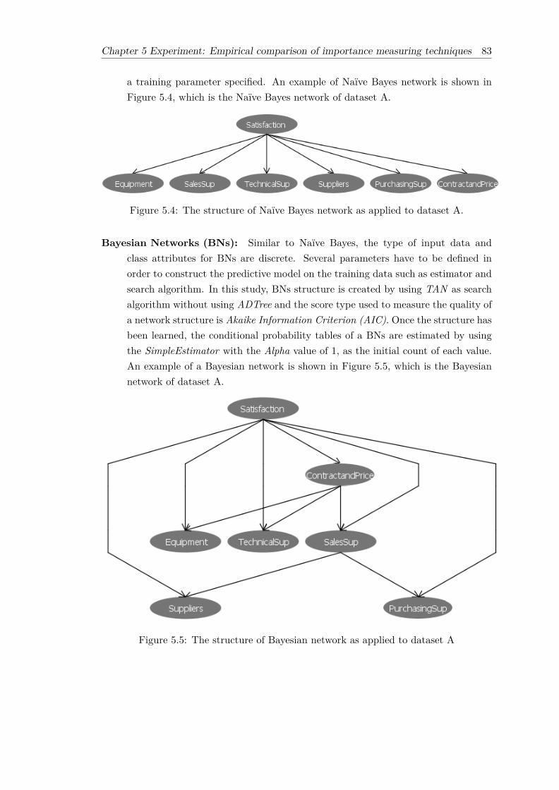
Chapter 5 Experiment: Empirical comparison of importance measuring techniques 83
a training parameter specified. An example of Naïve Bayes network is shown inFigure 5.4, which is the Naïve Bayes network of dataset A.
Figure 5.4: The structure of Naïve Bayes network as applied to dataset A.
Bayesian Networks (BNs): Similar to Naïve Bayes, the type of input data andclass attributes for BNs are discrete. Several parameters have to be defined inorder to construct the predictive model on the training data such as estimator andsearch algorithm. In this study, BNs structure is created by using TAN as searchalgorithm without using ADTree and the score type used to measure the quality ofa network structure is Akaike Information Criterion (AIC). Once the structure hasbeen learned, the conditional probability tables of a BNs are estimated by usingthe SimpleEstimator with the Alpha value of 1, as the initial count of each value.An example of a Bayesian network is shown in Figure 5.5, which is the Bayesiannetwork of dataset A.
Figure 5.5: The structure of Bayesian network as applied to dataset A
84 Chapter 5 Experiment: Empirical comparison of importance measuring techniques
5.4.2.2 Model quality
The quality of the model training may affect how well different techniques measure theimportance since it will be derived from these models. Therefore, the quality of themodel training in the previous sub-section will be evaluated in this section. In thisexperiment the quality of the model is measured in terms of accuracy (percentage ofcorrect classification rate) and Root Mean Squared Error (RMSE) measured in trainingmode and testing mode that used 10-fold cross validation.
For each dataset, accuracy and RMSE of the model using different techniques will becompared against the baseline techniques namely ZeroR and OneR (Witten and Frank,2005). As its name, ZeroR predicts class by considering only the class attribute (ignoreinput attributes). Class is assigned as the mean (for a numeric class) or the mode(for a nominal class). OneR predicts class by considering one attribute that yields theminimum-error for prediction.
Since accuracy is measured as percentage of correct classification rate, the higher accu-racy is preferred to the lower one. Conversely, RMSE measures how much the predictedvalue differs from the actual value, therefore the lower RMSE is preferred to the higherone. In other word, the closer the RMSE is to zero, the more accurate the model is.It is expected that all selected techniques yield higher accuracy and lower RMSE thanthe two baseline techniques in both training and testing mode. Accuracy and RMSE ofmodels of different techniques is shown in Table 5.6 - 5.8, for dataset A to dataset Crespectively. Accuracy and RMSE comparison of models across three datasets is shownin Figure 5.6 and Figure 5.7.
According to the average accuracy of models shown in Table 5.6 - 5.8 and Figure 5.6,all models of the selected techniques yielded higher accuracy than the baseline accu-racy produced by ZeroR. There is no dominating model that yields highest accuracyconsistently across three dataset. BNs yielded the highest accuracy in dataset A whileBPNN(classification) yielded the highest accuracy in the last two datasets. Among theselected techniques, OLR model yielded the lowest accuracy in dataset A and datasetC, while Naïve Bayes yielded the lowest accuracy in dataset B. The accuracy of thesetwo models was lower than or equal to the accuracy of OneR, another baseline model,in the specified datasets.
Based on the average RMSE of models shown in Table 5.6 - 5.8 and Figure 5.7, itcan clearly be seen that the model of MLR and BPNN(regression) yielded much highererror in terms of RMSE than the baseline RMSE (ZeroR and OneR) and models of theother techniques. MLR yielded the highest error rate across three datasets. BNs, OLR,and BPNN(classification) yielded the lowest error rate in terms of RMSE in dataset A,dataset B and dataset C respectively.

Chapter 5 Experiment: Empirical comparison of importance measuring techniques 85
Table 5.6: Accuracy and RMSE of models using different techniques on datasetA
Model Train Test Average(10-fold cross validation)
Accuracy RMSE Accuracy RMSE Accuracy RMSEZeroR 44.70% 0.34 44.70% 0.34 44.70% 0.34
OneR 56.06% 0.38 54.92% 0.39 55.49% 0.39
MLR - 0.79 - 0.82 - 0.81
OLR 54.17% 0.32 49.24% 0.40 51.71% 0.36
BPNN - 0.77 - 0.80 - 0.79
(regression)
BPNN 65.53% 0.28 46.97% 0.35 56.25% 0.32(classification)
Naïve Bayes 62.50% 0.29 53.03% 0.32 57.77% 0.31
BNs 72.73% 0.25 53.41% 0.32 63.07% 0.29
Table 5.7: Accuracy and RMSE of models using different techniques on datasetB
Model Train Test Average(10-fold cross validation)
Accuracy RMSE Accuracy RMSE Accuracy RMSEZeroR 68.62% 0.27 68.62% 0.29 68.62% 0.28
OneR 70.84% 0.31 69.89% 0.32 70.37% 0.32
MLR - 0.51 - 0.51 - 0.51
OLR 70.47% 0.26 70.62% 0.26 70.55% 0.26
BPNN - 0.50 - 0.50 - 0.50
(regression)
BPNN 74.56% 0.28 70.22% 0.26 72.39% 0.27(classification)
Naïve Bayes 58.40% 0.36 57.80% 0.38 58.10% 0.37
BNs 73.20% 0.25 67.38% 0.28 70.29% 0.27

86 Chapter 5 Experiment: Empirical comparison of importance measuring techniques
Table 5.8: Accuracy and RMSE of models using different techniques on datasetC
Model Train Test Average(10-fold cross validation)
Accuracy RMSE Accuracy RMSE Accuracy RMSEZeroR 63.87% 0.32 63.87% 0.32 63.87% 0.32
OneR 77.42% 0.30 76.77% 0.31 77.10% 0.31
MLR - 0.38 - 0.73 - 0.55
OLR 82.58% 0.31 71.62% 0.40 77.10% 0.35
BPNN - 0.37 - 0.40 - 0.39
(regression)
BPNN 90.97% 0.18 80.00% 0.26 85.49% 0.22(classification)
Naïve Bayes 83.23% 0.24 81.29% 0.25 82.26% 0.25
BNs 86.45% 0.21 80.00% 0.25 83.23% 0.23
As a model which has a higher accuracy and lower error rate is preferable, two models:BNs and BPNN(classification) produced superior model quality than the other models.Both models consistently produced the highest accuracy and lowest RMSE across thethree datasets. OLR and Naïve Bayes produced a moderate model quality. Althoughthese two models produced model accuracy lower than or equal to that of OneR insome datasets, they yielded satisfactory RMSE. MLR and BPNN(regression) produceda low model quality, since both models yielded RMSE higher than the baseline RMSE.Notably, their RMSE measured on dataset A is considerably higher.
5.4.3 Obtaining importance
Recall that different techniques are categorized into three groups which are self-statedimportance, statistically inferred importance and data mining implicitly derived impor-tance. Each group has its own approach to obtain importance. For the direct-ratingscales (DR) which is self-stated importance technique, the importance is calculatedstraightforwardly as the mean importance of each attribute. For the statistically inferredimportance techniques, MLR and OLR, the coefficients of these two regression modelscan be referred to as implicit importance which expresses the influence of attributes onthe overall customer satisfaction.
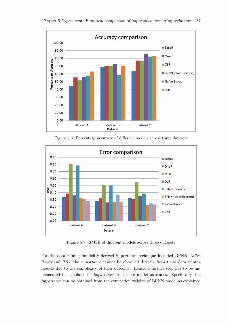
Chapter 5 Experiment: Empirical comparison of importance measuring techniques 87
Figure 5.6: Percentage accuracy of different models across three datasets
Figure 5.7: RMSE of different models across three datasets
For the data mining implicitly derived importance technique included BPNN, NaïveBayes and BNs, the importance cannot be obtained directly from these data miningmodels due to the complexity of their outcome. Hence, a further step has to be im-plemented to calculate the importance from these model outcomes. Specifically, theimportance can be obtained from the connection weights of BPNN model as explained

88 Chapter 5 Experiment: Empirical comparison of importance measuring techniques
in Step 2 of Section 3.3.3. The importance can be obtained from the conditional prob-ability table of Naïve Bayes and BNs model as explained in Step 2 of Section 3.3.4 andSection 3.3.5. The computational example of importance obtained from Dataset A canbe found in Appendix F.
For the purpose of comparison of the different importance measures, all the importancemeasured by each technique were expressed as a percentage contribution of attribute,with the negative importance estimated by MLR and OLR set to zero. This approach wasused in previous comparative studies of importance measures (Gustafsson and Johnson,2004; Pokryshevskaya and Antipov, 2014). In detail, the percentage contribution foreach attribute x is calculated as the proportion of raw importance of attribute x tothe summation of raw importance of all attributes. The importance obtained by eachtechnique from the three datasets is shown in Table 5.9 - 5.11. The highest importancemeasure is represented as bold while the least importance measure is underlined.
Table 5.9: Importance measured by using different techniques on dataset A(percentage). Values in bold are the highest importance measure while valuesunderlined are the lowest importance measure.
Attribute DR MLR OLR BPNN BPNN Naïve BNs(1) (2) Bayes
Equipment and System 17.24 18.77 17.41 20.23 28.90 22.52 20.41Sales Support 16.00 6.67 5.50 12.19 13.49 12.42 3.58Technical Support 17.68 40.82 47.10 25.59 19.06 22.80 20.40Supplies and Orders 16.70 14.97 12.89 14.33 8.79 14.36 13.66Purchasing Support 15.40 0.00 0.00 9.32 7.71 10.21 7.43Contracts and Pricing 16.97 18.77 17.11 18.34 22.04 17.69 34.51(1) regression, (2) classification
MLR, OLR and BPNN(regression) constantly identify the same most important at-tribute (formatted as a bold font) across three datasets which are “Technical support”,“efficiency of products/services” and “Extra-curricular Activity”. Naïve Bayes identi-fies the same most important attribute as those three techniques on dataset A anddataset B whereas BPNN(classification) identifies the same most important attributeas those three techniques only on dataset C. BNs identifies differently the most impor-tant attribute from the other techniques across three datasets which are “Contracts andPricing”, “problem solving” and “Computer Facility”.
Different techniques identify the least important attribute (formatted as underline) dif-ferently in three datasets. For dataset A, all techniques except BNs identify “PurchasingSupport” as the least important attribute. For dataset B, MLR and OLR identify twoattributes namely “expertise of personnel” and “helpfulness of personnel” as the leastimportant attribute. BNs identifies “expertise of personnel” as the joint least importantattribute with MLR and OLR, whereas BPNN(classification) and Naïve Bayes iden-tify “helpfulness of personnel” as the least important attribute as do MLR and OLR.

Chapter 5 Experiment: Empirical comparison of importance measuring techniques 89
Table5.10:
Impo
rtan
cemeasuredby
usingdiffe
rent
techniqu
eson
datasetB
(percentag
e).Va
lues
inbo
ldarethehigh
est
impo
rtan
cemeasure
while
values
underlinedarethelowe
stim
port
ance
measure.
Attribu
teDR
MLR
OLR
BPNN
BPNN
Naïve
BNs
(1)
(2)
Bayes
V42-exp
ertis
eof
person
nel
7.60
0.00
0.00
7.23
6.63
4.97
2.82
V43-con
sulting
servicecapa
bility
7.58
5.06
0.98
7.12
7.63
6.14
5.03
V44-problem
solving
7.91
9.07
14.38
7.37
6.24
7.23
27.66
V45-r
eliabilityof
prod
ucts/services
7.92
10.48
2.59
9.11
9.47
8.35
5.31
V46-flexibility
ofprod
ucts/services
7.48
5.18
5.82
4.30
8.42
8.91
6.21
V47-efficiency
ofprod
ucts/services
7.85
22.73
21.36
15.3
8.54
9.47
9.46
V48-w
orking
speedof
prod
ucts
7.76
8.60
12.86
4.62
6.10
8.67
8.65
V49-helpfulness
ofpe
rson
nel
7.62
0.00
0.00
12.28
5.46
4.91
2.84
V50-efficiency
inservingcustom
ers
7.70
1.18
3.01
6.27
8.83
7.28
6.39
V51-predisposition
towa
rdscustom
ers’
needs
7.54
3.18
6.22
5.75
6.93
7.99
4.75
V52-cap
acity
torespon
dto
custom
er’s
needs
7.74
15.67
17.81
7.38
6.03
8.98
8.98
V53-flexibility
inmak
ingchan
ges
7.59
4.71
4.57
2.19
8.19
8.43
5.17
V54-cap
acity
fortechno
logicalinn
ovation
7.71
14.13
10.39
11.08
11.53
8.67
6.74
(1)regressio
n,(2)classifi
catio
n

90 Chapter 5 Experiment: Empirical comparison of importance measuring techniques
Table 5.11: Importance measured by using different techniques on dataset C(percentage). Values in bold are the highest importance measure while valuesunderlined are the lowest importance measure.
Attribute DR MLR OLR BPNN BPNN Naïve BNs(1) (2) Bayes
Teacher 17.45 15.84 27.43 20.50 10.47 14.57 11.65Teaching 16.79 27.27 21.51 27.88 21.99 22.28 18.50Administration 16.75 8.17 1.73 5.28 11.23 14.13 9.55Computer Facility 17.23 3.52 13.20 9.49 15.18 14.02 31.72Additional Service 16.24 9.60 5.71 7.26 13.96 14.26 8.20Extra-curricular 15.55 35.60 30.43 29.59 27.17 20.74 20.38Activity(1) regression, (2) classification
The other techniques: direct-rating scales and BPNN(regression) identify “flexibility ofproducts/services” and “flexibility in making changes” as the least important attributerespectively. For dataset C, MLR and Naïve Bayes identify “Computer Facility” asthe least important attribute whereas OLR and BPNN(regression) identify “Admin-istration” as the least important attribute. Direct-rating scales, BPNN(classification)and BNs identify different attributes as the least important attribute which are “Extra-curricular Activity”, “Teacher” and “Additional Service”.
5.5 Summary
This chapter reports details of a comparative experiment which was conducted to selectthe technique to be used in the framework for conducting a SWOT analysis based on IPAas well as to help answer the first research question. First, the methodology of the twobaseline experiments was explained and results of these baseline experiments suggestedthat the comparative experiment was properly conducted. Then, the three evaluationmetrics for determining the best importance measure technique were described whichincluded the method for calculating their value and their interpretation. Each evaluationmetric evaluates each key aspect of importance measuring such as ability to discriminatethe most importance attribute, and it was selected from commonly used evaluation met-rics of previous comparative studies. Next, three datasets about customer satisfactionsurvey used in the comparative experiment were explained. Two datasets have beenused by other research, while another dataset was collected from a leading Universityin Thailand for the purpose of this study. The main characteristic of data for applyingIPA is containing an assessment of respondents’ satisfaction for a company’s productor service which is measured by Likert scales and containing an assessment of overallsatisfaction on the Likert scales.

Chapter 5 Experiment: Empirical comparison of importance measuring techniques 91
Lastly, procedures and techniques used in this comparative study were described. Thetechniques for measuring importance being investigated are direct-rating scales, MLR,OLR, BPNN, Naïve Bayes and BNs. To compare the different importance measures,firstly the datasets have to be pre-processed. Secondly, importance is obtained from thedatasets. For the direct-rating scales which is the self-stated importance method, theimportance is calculated straightforwardly as the mean importance of each attribute. Forthe derived importance technique: MLR, OLR, BPNN, Naïve Bayes and BNs, the modelof these techniques had to be implemented through the data analysis (model training)and evaluated using 10-fold cross validation. Then the importance was derived from theoutcomes of these models.
The importance measures obtained from different techniques identify differently the mostimportant and the least important attributes. The next chapter will present the compar-ative results of the importance measurement techniques based on the three evaluationmetrics. This leads to the justification to select the proper importance measurementtechnique.


Chapter 6
Results and Discussion:Empirical comparison ofimportance measuring
Given the three evaluation metrics and importance measures obtained from methodologyexplained in the previous chapter, this chapter presents the comparative results of thesix importance measuring techniques and statistical analysis of the empirical comparisonresults. These results will help answer research question 1 and lead to the decision toselect the technique to be used for measuring importance in the IPA based SWOTanalysis framework.
This chapter is organised as follows: section 6.1 reports the test of convergent validityof all importance measures. Section 6.2 describes the comparative results followed bystatistical analysis of these results (Section 6.3). Section 6.4 discusses the findings ofthis comparative experiment and section 6.5 provides the summary of the chapter.
6.1 The test of convergent validity of different importancemeasure
This section describes the result of the convergent validity of different importance mea-sures tested on the three datasets and the findings based on these results.
6.1.1 Results of convergent validity for each dataset
To investigate whether different importance measures reflect the same construct, the testof convergent validity among techniques for measuring attribute importance is conducted
93
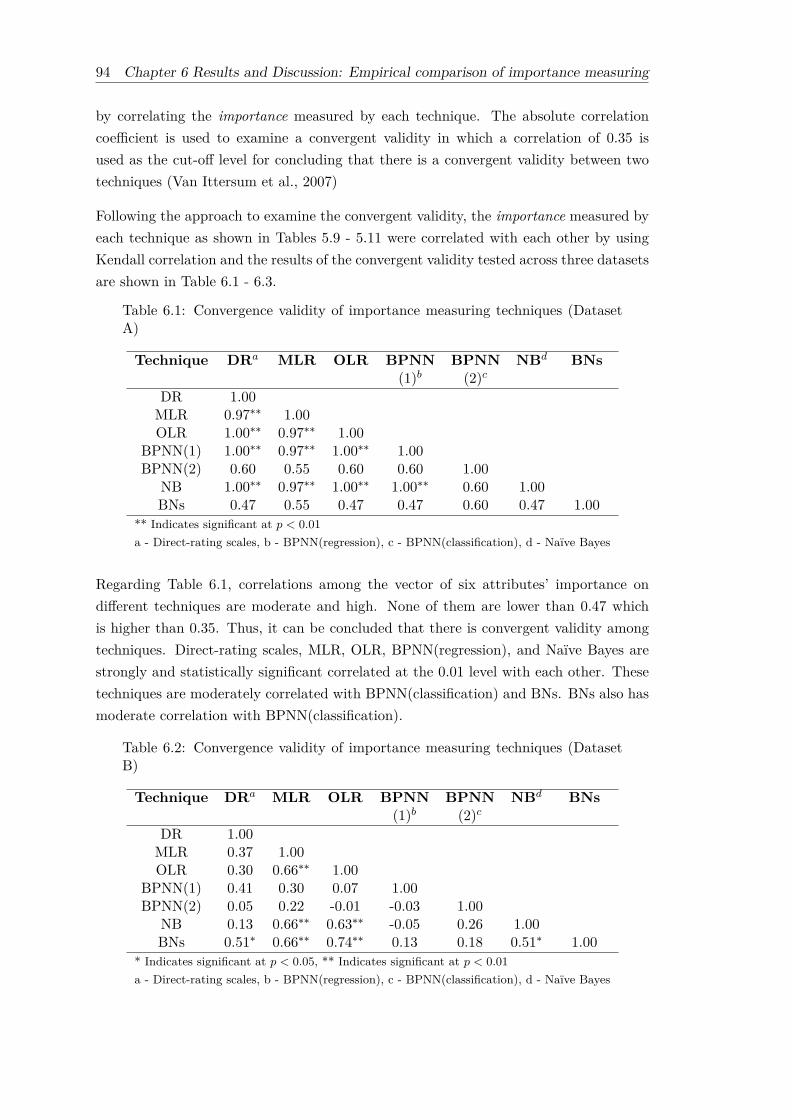
94 Chapter 6 Results and Discussion: Empirical comparison of importance measuring
by correlating the importance measured by each technique. The absolute correlationcoefficient is used to examine a convergent validity in which a correlation of 0.35 isused as the cut-off level for concluding that there is a convergent validity between twotechniques (Van Ittersum et al., 2007)
Following the approach to examine the convergent validity, the importance measured byeach technique as shown in Tables 5.9 - 5.11 were correlated with each other by usingKendall correlation and the results of the convergent validity tested across three datasetsare shown in Table 6.1 - 6.3.
Table 6.1: Convergence validity of importance measuring techniques (DatasetA)
Technique DRa MLR OLR BPNN BPNN NBd BNs(1)b (2)c
DR 1.00MLR 0.97∗∗ 1.00OLR 1.00∗∗ 0.97∗∗ 1.00
BPNN(1) 1.00∗∗ 0.97∗∗ 1.00∗∗ 1.00BPNN(2) 0.60 0.55 0.60 0.60 1.00
NB 1.00∗∗ 0.97∗∗ 1.00∗∗ 1.00∗∗ 0.60 1.00BNs 0.47 0.55 0.47 0.47 0.60 0.47 1.00
** Indicates significant at p < 0.01
a - Direct-rating scales, b - BPNN(regression), c - BPNN(classification), d - Naïve Bayes
Regarding Table 6.1, correlations among the vector of six attributes’ importance ondifferent techniques are moderate and high. None of them are lower than 0.47 whichis higher than 0.35. Thus, it can be concluded that there is convergent validity amongtechniques. Direct-rating scales, MLR, OLR, BPNN(regression), and Naïve Bayes arestrongly and statistically significant correlated at the 0.01 level with each other. Thesetechniques are moderately correlated with BPNN(classification) and BNs. BNs also hasmoderate correlation with BPNN(classification).
Table 6.2: Convergence validity of importance measuring techniques (DatasetB)
Technique DRa MLR OLR BPNN BPNN NBd BNs(1)b (2)c
DR 1.00MLR 0.37 1.00OLR 0.30 0.66∗∗ 1.00
BPNN(1) 0.41 0.30 0.07 1.00BPNN(2) 0.05 0.22 -0.01 -0.03 1.00
NB 0.13 0.66∗∗ 0.63∗∗ -0.05 0.26 1.00BNs 0.51∗ 0.66∗∗ 0.74∗∗ 0.13 0.18 0.51∗ 1.00
* Indicates significant at p < 0.05, ** Indicates significant at p < 0.01
a - Direct-rating scales, b - BPNN(regression), c - BPNN(classification), d - Naïve Bayes
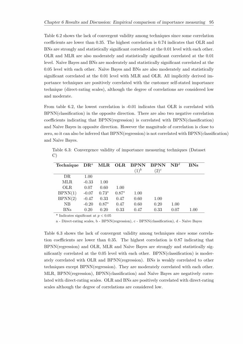
Chapter 6 Results and Discussion: Empirical comparison of importance measuring 95
Table 6.2 shows the lack of convergent validity among techniques since some correlationcoefficients are lower than 0.35. The highest correlation is 0.74 indicates that OLR andBNs are strongly and statistically significant correlated at the 0.01 level with each other.OLR and MLR are also moderately and statistically significant correlated at the 0.01level. Naïve Bayes and BNs are moderately and statistically significant correlated at the0.05 level with each other. Naïve Bayes and BNs are also moderately and statisticallysignificant correlated at the 0.01 level with MLR and OLR. All implicitly derived im-portance techniques are positively correlated with the customer self-stated importancetechnique (direct-rating scales), although the degree of correlations are considered lowand moderate.
From table 6.2, the lowest correlation is -0.01 indicates that OLR is correlated withBPNN(classification) in the opposite direction. There are also two negative correlationcoefficients indicating that BPNN(regression) is correlated with BPNN(classification)and Naïve Bayes in opposite direction. However the magnitude of correlation is close tozero, so it can also be inferred that BPNN(regression) is not correlated with BPNN(classification)and Naïve Bayes.
Table 6.3: Convergence validity of importance measuring techniques (DatasetC)
Technique DRa MLR OLR BPNN BPNN NBd BNs(1)b (2)c
DR 1.00MLR -0.33 1.00OLR 0.07 0.60 1.00
BPNN(1) -0.07 0.73∗ 0.87∗ 1.00BPNN(2) -0.47 0.33 0.47 0.60 1.00
NB -0.20 0.87∗ 0.47 0.60 0.20 1.00BNs 0.20 0.20 0.33 0.47 0.33 0.07 1.00
* Indicates significant at p < 0.05
a - Direct-rating scales, b - BPNN(regression), c - BPNN(classification), d - Naïve Bayes
Table 6.3 shows the lack of convergent validity among techniques since some correla-tion coefficients are lower than 0.35. The highest correlation is 0.87 indicating thatBPNN(regression) and OLR, MLR and Naïve Bayes are strongly and statistically sig-nificantly correlated at the 0.05 level with each other. BPNN(classification) is moder-ately correlated with OLR and BPNN(regression). BNs is weakly correlated to othertechniques except BPNN(regression). They are moderately correlated with each other.MLR, BPNN(regression), BPNN(classification) and Naïve Bayes are negatively corre-lated with direct-rating scales. OLR and BNs are positively correlated with direct-ratingscales although the degree of correlations are considered low.

96 Chapter 6 Results and Discussion: Empirical comparison of importance measuring
6.1.2 Convergent Validity Findings
The test of convergent validity across the three datasets yielded mixed results. Only theconvergent validity test on dataset A shows the convergent validity among the impor-tance measured techniques, whereas other convergent validity tests showed the lack ofconvergent validity among the importance measured techniques. Considering the corre-lation between a pair of techniques, MLR and OLR are consistently strongly or mod-erately correlated with each other across the convergent validity test on three datasets.None of the correlation coefficients between MLR and OLR are lower than 0.35 whichdemonstrates the convergent validity between these two techniques. The convergentvalidity between MLR and OLR corresponds to the ground theory of them since, OLRis an extension of a logistic regression which is analogous to a linear regression. Theresult of convergent validity is also harmonized with the rank of attribute importanceof these two techniques as they identified the same most important attribute in threedatasets and identified the same least important attribute in two out of three datasets.
The convergent validity tested on dataset A and dataset C demonstrates the convergentvalidity between BPNN(regression) and BPNN(classification) since they are moderatelycorrelated with each other. Both BPNN(regression) and BPNN(classification) are themodel based on the Back Propagation Neural Network, however; BPNN(regression) hasa higher correlation with MLR and OLR than with BPNN(classification), as shownin Tables 6.1-6.3. Since BPNN can be considered as an advance version of MLR andBPNN(regression) treating the dependent variable as quantitative discrete in the sameway as MLR, whereas BPNN(classification) treats the dependent variable as categorical.Thereby, these two models of BPNN used different activation functions in the outputlayer: identity versus logistic function.
Although Naïve Bayes can be considered as a special case of BNs (Grossman and Domin-gos, 2004) and these two techniques are also treated the dependent variable as categori-cal, Naïve Bayes has a higher correlation with MLR and OLR than with BNs. As shownin Table 6.1-6.3, Naïve Bayes is consistently strongly or moderately correlated with MLRand OLR across the convergent validity tested on three datasets. However Naïve Bayesis moderately or weakly correlated with BNs with one of the tests of convergent validitywhich shows the lack of convergent validity between them.
Considering the convergent validity among groups of different techniques, customer self-stated and all implicitly derived importance measures which are statistically inferredimportance and data mining implicitly derived importance, seem to have low convergentvalidity. Only the convergent validity tested on dataset A demonstrates the convergentvalidity among them. Other of them shows the lack of convergent validity. This supportsthe result of Tontini et al. (2014) that reported the lack of convergent validity betweenthe customer self-stated importance and indirect importance measures (calculated usingprincipal component regression). Among the implicitly derived importance measure

Chapter 6 Results and Discussion: Empirical comparison of importance measuring 97
techniques, BNs is the only technique that is consistently positively correlated withdirect-rating scales across the convergent validity tested on three datasets.
These results lead to the conclusions that MLR and OLR produces similar importancemeasures. BPNN(regression) and Naïve Bayes produces importance measures closelyagreeing to that of MLR and OLR. All implicitly derived importance measures tend toyield different importance measures from the customer self-stated measures. Anotherinteresting finding is that a different data type of the dependent variable required byeach technique does not directly effect the convergent validity among techniques. Forexample, MLR and OLR treat the dependent variable in different type but there ishigh convergent validity between them. In contrast, both Naïve Bayes and BNs treatthe dependent variable as categorical but there is a lack of convergent validity betweenthem.
6.2 Result of the empirical comparison
Importance measured by the six techniques, described in Sub-section 5.4.3 of the previouschapter, was tested against the three evaluation metrics, described in Section 5.2 of theprevious chapter by using SPSS. The comparison results will be described in the followingsub-sections.
6.2.1 Predictive validity
The analysis of predictive validity was evaluated in respondent-level data by correlatingan actual overall customer satisfaction with the predicted overall customer satisfactioncomputed as a multi-attribute attitude model. The results of predictive validity testedacross three datasets are shown in Table 6.4 .
Table 6.4: A measure of predictive validity as correlation coefficient betweenmulti-attribute attitude model predictions with overall satisfaction. The highercorrelation coefficient (close to 1) indicates the better predictive validity.
Technique Dataset A Dataset B Dataset C AverageSatisfaction rating* 0.585 0.633 0.760 0.659Direct-rating scales 0.593 0.633 0.759 0.662MLR 0.660 0.651 0.781 0.697OLR 0.657 0.649 0.773 0.693BPNN(regression) 0.634 0.631 0.779 0.681BPNN(classification) 0.609 0.637 0.769 0.672Naïve Bayes 0.626 0.640 0.768 0.678BNs 0.617 0.633 0.746 0.665*Baseline measurement of predictive validity

98 Chapter 6 Results and Discussion: Empirical comparison of importance measuring
With regard to the correlation coefficients shown in Table 6.4, all techniques produceda positive correlation coefficient indicating that satisfaction levels of attributes are pos-itively related with overall customer satisfaction. All correlation coefficients are statis-tically significant at the 0.01 level (1-tailed). These correlation coefficients ranged from0.58 to 0.78 indicating that correlations of multi-attribute attitude model predictionswith overall customer satisfaction are moderate and high. In other words, all techniqueshave a good predictive validity.
None of the techniques for measuring importance yield the average correlation coeffi-cient across three datasets lower than the average correlation coefficient of the baselinepredictive validity which is computed as multi-attribute attitude model without impor-tance. Thus it clearly shows that the importance obtained from these techniques is avalid indicator of the overall customer satisfaction.
Based on the average correlation coefficient across three datasets, MLR yielded the high-est correlation coefficient closely followed by OLR and the lowest correlation coefficientbelongs to direct-rating scales which is slightly higher than the baseline correlation co-efficient. Thus it can be concluded that MLR has a superior predictive validity thanother techniques. However, the correlation of MLR has insignificant cardinal differencesfrom that of other techniques especially OLR.
6.2.2 Diagnosticity
According to Pokryshevskaya and Antipov (2014)’s approach for evaluating diagnostic-ity, the importance measures obtained from each technique were regressed with rankresulting in the non-linear regression coefficients shown in Table 6.5.
Table 6.5: A measure of diagnosticity as non-linear regression coefficient (β2) ofthe relationship between importance and rank. The lower the value of non-linearregression coefficient indicates the better diagnosticity.
Technique Dataset A Dataset B Dataset CDirect-rating scales 0.58 -0.06 0.62MLR -19.21 -7.36*** -15.79OLR -34.86 -6.34*** 5.34BPNN(regression) -3.87 -3.51** -1.38BPNN(classification) -6.02 -1.54** -10.72*Naïve Bayes 0.94 1.34* -7.95BNs -10.34** -14.71** -14.99** Indicates significant at p < 0.05
** Indicates significant at p < 0.01
*** Indicates significant at p < 0.001
As the lower the value of non-linear regression coefficient indicates the better abilityto differentiate the important attribute, OLR has the highest ability to diagnose the
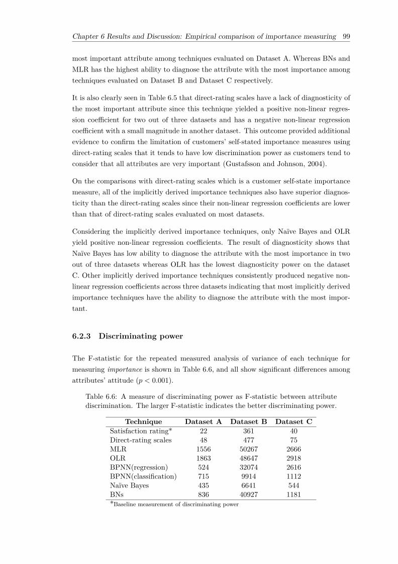
Chapter 6 Results and Discussion: Empirical comparison of importance measuring 99
most important attribute among techniques evaluated on Dataset A. Whereas BNs andMLR has the highest ability to diagnose the attribute with the most importance amongtechniques evaluated on Dataset B and Dataset C respectively.
It is also clearly seen in Table 6.5 that direct-rating scales have a lack of diagnosticity ofthe most important attribute since this technique yielded a positive non-linear regres-sion coefficient for two out of three datasets and has a negative non-linear regressioncoefficient with a small magnitude in another dataset. This outcome provided additionalevidence to confirm the limitation of customers’ self-stated importance measures usingdirect-rating scales that it tends to have low discrimination power as customers tend toconsider that all attributes are very important (Gustafsson and Johnson, 2004).
On the comparisons with direct-rating scales which is a customer self-state importancemeasure, all of the implicitly derived importance techniques also have superior diagnos-ticity than the direct-rating scales since their non-linear regression coefficients are lowerthan that of direct-rating scales evaluated on most datasets.
Considering the implicitly derived importance techniques, only Naïve Bayes and OLRyield positive non-linear regression coefficients. The result of diagnosticity shows thatNaïve Bayes has low ability to diagnose the attribute with the most importance in twoout of three datasets whereas OLR has the lowest diagnosticity power on the datasetC. Other implicitly derived importance techniques consistently produced negative non-linear regression coefficients across three datasets indicating that most implicitly derivedimportance techniques have the ability to diagnose the attribute with the most impor-tant.
6.2.3 Discriminating power
The F-statistic for the repeated measured analysis of variance of each technique formeasuring importance is shown in Table 6.6, and all show significant differences amongattributes’ attitude (p < 0.001).
Table 6.6: A measure of discriminating power as F-statistic between attributediscrimination. The larger F-statistic indicates the better discriminating power.
Technique Dataset A Dataset B Dataset CSatisfaction rating* 22 361 40Direct-rating scales 48 477 75MLR 1556 50267 2666OLR 1863 48647 2918BPNN(regression) 524 32074 2616BPNN(classification) 715 9914 1112Naïve Bayes 435 6641 544BNs 836 40927 1181*Baseline measurement of discriminating power

100 Chapter 6 Results and Discussion: Empirical comparison of importance measuring
None of the techniques for measuring importance yield an F-statistic lower than baselineF-statistic which means attributes’ importance acquired from each technique increasethe size of difference between attributes’ attitude. All implicitly derived importancetechniques yield significant cardinal differences of F-statistic from the baseline F-statisticacross all three datasets.
Recall that the larger F-statistic, indicates the more differentiation between attributesand a smaller F-statistic means less. Two techniques, MLR and OLR, clearly stand outas producing much larger values than the other measures. Specifically, OLR yieldedthe largest F-statistic in two out of three datasets which are dataset A and Dataset Cwhile MLR yielded the largest F-statistic in dataset B. BNs yielded the third largestF-statistic in two out of three datasets. The direct-rating scales produced the lowestF-statistic which is close to the baseline F-statistic.
6.2.4 Summary of comparative results
Ranking of the techniques according to their predictive validity, diagnosticity and dis-criminating power presented in Table 6.7 (rank 1 corresponds to the best technique, rank7– to the worst one), indicated that there is no clear winning technique since no onetechnique outperforms all the others across three metrics. MLR has the best predictivevalidity and diagnosticity whereas OLR has the best discrimination. However, consid-ering the average rank of three evaluation metrics in Table 6.7 leads to the followingfindings which help answer the first research question:
(1) MLR is the best importance measurement technique based on the average rankof three evaluation metrics since it has the best predictive validity and diagnosticitypower, and the second best discriminating power. OLR is the second best importancemeasurement technique as it has the best discriminating power and its predictive validityis nearly as good as MLR and its diagnosticity power is also ranked after MLR. BNs isthe third best importance measurement technique as it has the second best diagnosticitypower and the third best discriminating power.
(2) Direct-rating scales is the worst importance measurement technique since it is rankedlast among the importance measurement techniques in all evaluation metrics. Based onthis finding, it clearly shows that the implicitly derived importance techniques are betterthan the customer self-stated importance technique in term of these three evaluationmetrics.
(3) Naïve Bayes is the second worst importance measurement technique and the worstimplicitly derived importance technique based on the average rank of three evaluationmetrics since, it has the lowest discriminative power and the lowest diagnosticity poweramong implicitly derived importance techniques and it has a moderate predictive valid-ity.

Chapter 6 Results and Discussion: Empirical comparison of importance measuring 101
(4) Considering two types of BPNN model, BPNN(regression) is ranked fourth whileBPNN(classification) is ranked fifth among the importance measurement techniquesbased on the average rank of three evaluation metrics. This indicated that BPNN(regression)outperforms BPNN(classification) in measuring importance.
The first and second finding reveal the best and the worse importance measurementtechniques based on the average rank of three evaluation metrics. These findings providethe answer to the first research question through its sub research questions. Specifically,the first finding provides the answer to sub research question 1.2 that MLR is themost appropriate technique for measuring importance. The second finding provides theanswer to sub research question 1.1 that implicitly derived importance works better inmeasuring importance than customer self-stated importance. The other findings revealthe techniques that are ranked between the best and the worse importance measurementtechnique.
6.3 Statistical analysis of the results for the empirical com-parison
To provide a statistical foundation for the findings in Section 6.2, the difference inthe three evaluation metrics were statistically tested. Each metric results in differenttypes of statistic which are correlation coefficients, regression coefficients and F-statisticsrespectively. Hence, the differences in the correlation coefficients, regression coefficientsand F-statistics were tested corresponded to each metric.
6.3.1 Statistical test of Predictive validity
For each dataset, the significance tests for differences in predictive ability were testedfollowing Williams’s t-test for testing equality of dependent correlation coefficients assuggested in Chen and Popovich (2002) since all correlations were computed based onthe same dataset and the sample size exceeds 20.
These differences in the correlations were tested in order to investigate whether theactual overall customer satisfaction (variable j) related to the predicted overall customersatisfaction of technique k were statistically significant different from that of techniqueh. The null hypothesis is stated as rjk = rjh and the alternative hypothesis is rjk = rjh
The test results are shown in Table 6.8 - 6.10 as absolute t-values of the significance testsfor differences in predictive validity for dataset A, B and C respectively. For each table,t-values represent the degree of difference between two correlation coefficients which isa measure of the predictive validity of the technique. The t-value of zero indicates no

102 Chapter 6 Results and Discussion: Empirical comparison of importance measuring
Table6.7:
The
rankingoftechniques
accordingto
thetree
evaluationmetrics
(The
lowerthe
rank,thebetter
theimportance
measure)
TechniqueRank
bypredictive
validityRank
bydiagnosticity
Rank
bydiscrim
inatingpow
erMean
ofRank
Dataset
Mean
Dataset
Mean
Dataset
Mean
allA
BC
Rank
AB
CRank
AB
CRank
metrics
Direct-rating
scales7
56
6.06
66
6.07
77
7.06.33
7MLR
11
11.0
22
11.7
21
21.7
1.441
OLR
22
32.3
13
73.7
12
11.3
2.442
BPNN(regression)
37
24.0
54
54.7
54
34.0
4.224
BPNN(classification)
64
44.7
45
34.0
45
54.7
4.445
Naïve
Bayes4
35
4.07
74
6.06
66
6.05.33
6BN
s5
57
5.73
12
2.03
34
3.33.67
3

Chapter 6 Results and Discussion: Empirical comparison of importance measuring 103
difference between predictive validity of the two techniques and the bigger the t-value,the more difference between predictive validity of the two techniques.
Additionally, to determine whether the difference between the predictive validity of thetwo techniques is statistically significant, the p-values of the tests were compared to thesignificance level of 0.05, 0.01 and 0.001. The symbol ‘*’ indicates that p-value is lessthan the significance level of 0.05, the symbol ‘**’ indicates that p-value is less thanthe significance level of 0.01 and the symbol ‘***’ indicates that p-value is less than thesignificance level of 0.001.
Table 6.8: Significance tests for differences in predictive ability (Dataset A)
Technique SRa DRb MLR OLR BPNN BPNN NBe BNs(1)c (2)d
SR -DR 3.67∗∗∗ -MLR 3.54∗∗∗ 3.36∗∗∗ -OLR 3.01∗∗ 2.81∗∗ 0.83 -
BPNN(1) 5.13∗∗∗ 5.09∗∗∗ 2.11∗ 1.50 -BPNN(2) 1.90 1.38 2.85∗∗ 2.28∗ 2.94∗∗ -
NB 4.87∗∗∗ 4.52∗∗∗ 2.39∗ 1.79 3.82∗∗∗ 2.39∗ -BNs 1.88 1.50 2.59∗ 2.04∗ 1.43 0.68 0.75 -
* Indicates significant at p < 0.05
** Indicates significant at p < 0.01
*** Indicates significant at p < 0.001
a - Satisfaction Rating (baseline measurement of predictive validity)b - Direct-rating scales, c - BPNN(regression), d - BPNN(classification), e - Naïve Bayes
Table 6.4 and Table 6.8 show that correlations of most techniques except BPNN(classification)and BNs are statistically significantly different to the correlation of the baseline predic-tive validity. These tables also show that the highest correlation which belongs to MLRis significantly higher than the correlation of other techniques except OLR, the secondbest predictive validity technique.
The first column of Table 6.9 shows that correlations of most techniques are statisticallysignificantly different to the baseline correlation except direct-rating scales and BNs sinceboth techniques yield exactly the same correlation coefficient as the baseline correlation.Table 6.4 and Table 6.9 show that the highest correlation which belongs to MLR isstatistically significantly higher than the correlation of other techniques at the 0.001
level of significance. These tables also show that the lowest correlation which belongs toBPNN(regression) is significantly lower than the correlation of other techniques exceptBNs. There are significantly differences between the correlations of techniques rankedin the top-5.
The first column of Table 6.10 shows that only the correlation produced by Naïve Bayes isstatistically significantly different to the baseline correlation. Other techniques producecorrelations that are not significantly different to baseline correlation. Considering the
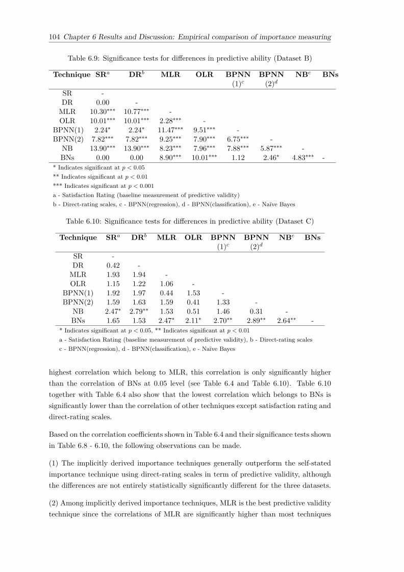
104 Chapter 6 Results and Discussion: Empirical comparison of importance measuring
Table 6.9: Significance tests for differences in predictive ability (Dataset B)
Technique SRa DRb MLR OLR BPNN BPNN NBe BNs(1)c (2)d
SR -DR 0.00 -MLR 10.30∗∗∗ 10.77∗∗∗ -OLR 10.01∗∗∗ 10.01∗∗∗ 2.28∗∗∗ -
BPNN(1) 2.24∗ 2.24∗ 11.47∗∗∗ 9.51∗∗∗ -BPNN(2) 7.82∗∗∗ 7.82∗∗∗ 9.25∗∗∗ 7.90∗∗∗ 6.75∗∗∗ -
NB 13.90∗∗∗ 13.90∗∗∗ 8.23∗∗∗ 7.96∗∗∗ 7.88∗∗∗ 5.87∗∗∗ -BNs 0.00 0.00 8.90∗∗∗ 10.01∗∗∗ 1.12 2.46∗ 4.83∗∗∗ -
* Indicates significant at p < 0.05
** Indicates significant at p < 0.01
*** Indicates significant at p < 0.001
a - Satisfaction Rating (baseline measurement of predictive validity)b - Direct-rating scales, c - BPNN(regression), d - BPNN(classification), e - Naïve Bayes
Table 6.10: Significance tests for differences in predictive ability (Dataset C)
Technique SRa DRb MLR OLR BPNN BPNN NBe BNs(1)c (2)d
SR -DR 0.42 -MLR 1.93 1.94 -OLR 1.15 1.22 1.06 -
BPNN(1) 1.92 1.97 0.44 1.53 -BPNN(2) 1.59 1.63 1.59 0.41 1.33 -
NB 2.47∗ 2.79∗∗ 1.53 0.51 1.46 0.31 -BNs 1.65 1.53 2.47∗ 2.11∗ 2.70∗∗ 2.89∗∗ 2.64∗∗ -
* Indicates significant at p < 0.05, ** Indicates significant at p < 0.01
a - Satisfaction Rating (baseline measurement of predictive validity), b - Direct-rating scalesc - BPNN(regression), d - BPNN(classification), e - Naïve Bayes
highest correlation which belong to MLR, this correlation is only significantly higherthan the correlation of BNs at 0.05 level (see Table 6.4 and Table 6.10). Table 6.10together with Table 6.4 also show that the lowest correlation which belongs to BNs issignificantly lower than the correlation of other techniques except satisfaction rating anddirect-rating scales.
Based on the correlation coefficients shown in Table 6.4 and their significance tests shownin Table 6.8 - 6.10, the following observations can be made.
(1) The implicitly derived importance techniques generally outperform the self-statedimportance technique using direct-rating scales in term of predictive validity, althoughthe differences are not entirely statistically significantly different for the three datasets.
(2) Among implicitly derived importance techniques, MLR is the best predictive validitytechnique since the correlations of MLR are significantly higher than most techniques

Chapter 6 Results and Discussion: Empirical comparison of importance measuring 105
tested on two out of three datasets.
(3) Among implicitly derived importance techniques, BNs seem to have a low predictivevalidity since its correlations are not statistically significantly different from the baselinecorrelation tested across three datasets.
6.3.2 Statistical test of Diagnosticity
For each dataset, the significance tests for differences in diagnosticity were tested fol-lowing an approach for the significance tests of two independent regression coefficientsdescribed in Kenny (1987) since the non-linear regression coefficients (Table 6.5) beingtested were computed from importance measures of different techniques.
The null hypothesis to be tested is that a pair of regression coefficients is not significantlydifferent from one another. This test of difference produces Student’s t-statistic withN-4 degree of freedom where N is the sample size of two groups.
Table 6.11 - 6.13 show absolute t-values of the significance tests for differences in regres-sion coefficients of dataset A, B and C respectively. T-values in each table represent thedegree of difference between two regression coefficients which is a measure of diagnostic-ity of the technique. The t-value of zero indicates no differences between diagnosticity ofthe two techniques and the bigger the t-value, the more difference between diagnosticityof the two techniques.
Additionally, to determine whether the difference between diagnosticity of the two tech-niques is statistically significant, the p-values of the tests were compared to the signif-icance level of 0.05, 0.01 and 0.001. The symbol ‘*’ indicates that p-value is less thanthe significance level of 0.05, the symbol ‘**’ indicates that p-value is less than thesignificance level of 0.01 and the symbol ‘***’ indicates that p-value is less than thesignificance level of 0.001.
Table 6.11: Significance tests for differences in diagnosticity (Dataset A)
Technique DRa MLR OLR BPNN BPNN NBd BNs(1)b (2)c
DR -MLR 1.54 -OLR 2.42∗ 0.80 -
BPNN(1) 2.47∗ 1.18 2.10 -BPNN(2) 1.97 0.99 1.92 0.57 -
NB 0.11 1.52 2.39∗ 1.28 1.48 -BNs 1.45 0.60 1.49 0.84 0.53 1.37 -
* Indicates significant at p < 0.05
a - Direct-rating scales, b - BPNN(regression), c - BPNN(classification), d - Naïve Bayes

106 Chapter 6 Results and Discussion: Empirical comparison of importance measuring
Table 6.12: Significance tests for differences in diagnosticity (Dataset B)
Technique DRa MLR OLR BPNN BPNN NBd BNs(1)b (2)c
DR -MLR 7.96∗∗∗ -OLR 6.17∗∗∗ 0.74 -
BPNN(1) 4.13∗∗∗ 3.11∗∗ 2.15∗ -BPNN(2) 4.16∗∗∗ 5.92∗∗∗ 4.45∗∗∗ 2.16∗ -
NB 2.81∗ 8.35∗∗∗ 6.78∗∗∗ 4.99∗∗∗ 4.72∗∗∗ -BNs 5.01∗∗∗ 2.40∗ 2.70∗ 3.68∗∗ 4.47∗∗∗ 5.41∗∗∗ -
* Indicates significant at p < 0.05
** Indicates significant at p < 0.01
*** Indicates significant at p < 0.001
a - Direct-rating scales, b - BPNN(regression), c - BPNN(classification), d - Naïve Bayes
Table 6.13: Significance tests for differences in diagnosticity (Dataset C)
Technique DRa MLR OLR BPNN BPNN NBd BNs(1)b (2)c
DR -MLR 2.72∗ -OLR 1.12 2.88∗ -
BPNN(1) 0.21 1.30 0.65 -BPNN(2) 3.42∗ 0.74 3.01∗ 0.94 -
NB 1.85 1.03 2.13 0.63 0.49 -BNs 3.56∗ 0.11 3.36∗ 1.32 0.78 1.11 -
* Indicates significant at p < 0.05
a - Direct-rating scales, b - BPNN(regression), c - BPNN(classification), d - Naïve Bayes
Among three datasets, only dataset B with 13 observations (number of attributes usedfor building regression model) clearly shows significant differences between two regressioncoefficients of techniques as shown in Table 6.12 whereas Table 6.11 and Table 6.13 showthat most regression coefficients of techniques tested on dataset A and dataset C werenot significantly different. Since the power of the test difference between two regressioncoefficients is quite low (Kenny, 1987), even if the magnitude of coefficients tested ondataset A and C (Table 6.5) were quite different: with only six observations, significantdifferences between two regression coefficients were difficult to detect.
Based on the non-linear regression coefficient shown in Table 6.5 and their significancetests on three datasets shown in Table 6.11 - Table 6.13, the following observations canbe made.
(1) Most implicitly derived importance techniques except Naïve Bayes generally havesuperior diagnosticity power than the self-stated importance technique using direct-rating scales, although the differences are not entirely significant different for the threedatasets.

Chapter 6 Results and Discussion: Empirical comparison of importance measuring 107
(2) Among implicitly derived importance techniques, MLR has the best diagnosticitypower technique closely followed by BNs since MLR yields the top-2 best diagnosticitypower while BNs yields the top-3 best diagnosticity power across the three datasets. Theregression coefficients of MLR and BNs are significantly different from that of direct-rating scales in two out of the three datasets.
(3) Among implicitly derived importance techniques, Naïve Bayes has the lowest di-agnosticity power since its magnitude of regression coefficients are lower than that ofother implicitly derived importance techniques, although the differences are not entirelysignificant different for the three datasets.
6.3.3 Statistical test of Discriminating power
For each dataset, the significance tests for differences in discriminating power measuredas F-statistics were tested by converting F-statistics to correlation coefficients (r) thenconducting a test for equality of independent correlation coefficient. To convert F-statistics to r, first a partial eta squared (η2p) known as a measure of effect size wascalculated from F-statistics using the formula described in Fritz et al. (2012). This η2p
can be also obtained directly from an output of SPSS.
Then r can be easily calculated as a square root of η2p since it is a version of eta squared(η2) which also known as the correlation ratio or R2, and both η2p and η2 yield the sameresult in one-way ANOVAs (Levine and Hullett, 2002). Table 6.14 shows η2p and r cor-responding to F-statistics which is a measure of discriminating power of each techniqueacross the three datasets. The closer the value of r to 1, the better discriminating power.
Table 6.14: partial eta squared and correlation coefficient corresponded to F-statistics of each technique
Technique Dataset A Dataset B Dataset Cη2p r η2p r η2p r
Satisfaction rating* 0.078 0.279 0.074 0.272 0.205 0.453Direct-rating scales 0.154 0.392 0.096 0.31 0.329 0.574MLR 0.855 0.925 0.918 0.958 0.945 0.972OLR 0.876 0.936 0.915 0.957 0.95 0.975BPNN(regression) 0.666 0.816 0.877 0.936 0.944 0.972BPNN(classification) 0.731 0.855 0.688 0.829 0.878 0.937Naïve Bayes 0.623 0.789 0.596 0.772 0.78 0.883BNs 0.761 0.872 0.901 0.949 0.885 0.941* Baseline measurement of discriminating power
After r of each technique was computed for each dataset, the test for equality of sev-eral (more than two) independent correlation coefficients was conducted following anapproach described in Kenny (1987). The null hypothesis is that the correlations com-puted in k groups are not significantly different from one another. This test of difference

108 Chapter 6 Results and Discussion: Empirical comparison of importance measuring
produces Chi-square statistic (χ2) with k − 1 degree of freedom, where k is the numberof correlation coefficients. If the Chi-square statistic exceeds the critical value in a Chi-squared distribution table, the null hypothesis is rejected otherwise the null hypothesisis retained.
In this study, eight groups of correlation coefficients were tested including the baselinecorrelation as shown in Table 6.14 therefore the degree of freedom was seven for allthree datasets. The result of the test for equality of several independent correlationcoefficients across three datasets is reported in Table 6.15.
Table 6.15: Chi-square statistic for the difference test of several independentcorrelations
χ2 df p-valueDataset A 485.41 7 < 0.001Dataset B 14737.04 7 < 0.001Dataset C 467.79 7 < 0.001
Table 6.15 shows that there is a significant difference among correlations produced byeach technique at the 0.001 level of significance. Thus the tests for the equality of twoindependent correlation coefficients were conducted in order to investigate that (1) thebaseline correlation as transform version of the F-statistic is statistically significantly dif-ferent from correlation coefficients computed from F-statistic of each technique, and (2)the correlation coefficient computed from highest F-statistic is statistically significantlydifferent from that of other techniques.
The tests for the equality of two independent correlation coefficients were conductedfollowing an approach described in Kenny (1987). The null hypothesis to be tested isthat the two correlation coefficients are not significantly different.
Table 6.16 - Table 6.18 show absolute z-values of the significance tests for differencesin correlations (shown in Table 6.14) obtained from F-statistics in dataset A, B andC respectively. Z-values in each table represent the degree of difference between twocorrelation coefficients in units of the standard deviation. The z-value of zero indicatesno difference between discriminating power of the two techniques and the bigger thez-value, the more difference between discriminating power of the two techniques
Additionally, to determine whether the difference between the discriminating power ofthe two techniques is statistically significant, the p-values of the tests were compared tothe significance level of 0.05, 0.01 and 0.001. The symbol ‘*’ indicates that p-value isless than the significance level of 0.05, the symbol ‘**’ indicates that p-value is less thanthe significance level of 0.01 and the symbol ‘***’ indicates that p-value is less than thesignificance level of 0.001.
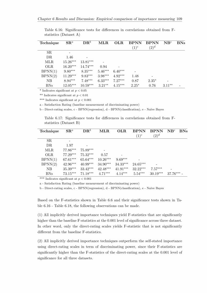
Chapter 6 Results and Discussion: Empirical comparison of importance measuring 109
Table 6.16: Significance tests for differences in correlations obtained from F-statistics (Dataset A)
Technique SRa DRb MLR OLR BPNN BPNN NBe BNs(1)c (2)d
SR -DR 1.46 -MLR 15.26∗∗∗ 13.81∗∗∗ -OLR 16.20∗∗∗ 14.74∗∗∗ 0.94 -
BPNN(1) 9.80∗∗∗ 8.35∗∗∗ 5.46∗∗∗ 6.40∗∗∗ -BPNN(2) 11.29∗∗∗ 9.83∗∗∗ 3.98∗∗∗ 4.92∗∗∗ 1.48 -
NB 8.94∗∗∗ 7.48∗∗∗ 6.33∗∗∗ 7.27∗∗∗ 0.87 2.35∗ -BNs 12.05∗∗∗ 10.59∗∗∗ 3.21∗∗ 4.15∗∗∗ 2.25∗ 0.76 3.11∗∗ -
* Indicates significant at p < 0.05
** Indicates significant at p < 0.01
*** Indicates significant at p < 0.001
a - Satisfaction Rating (baseline measurement of discriminating power)b - Direct-rating scales, c - BPNN(regression), d - BPNN(classification), e - Naïve Bayes
Table 6.17: Significance tests for differences in correlations obtained from F-statistics (Dataset B)
Technique SRa DRb MLR OLR BPNN BPNN NBe BNs(1)c (2)d
SR -DR 1.97 -MLR 77.86∗∗∗ 75.89∗∗∗ -OLR 77.29∗∗∗ 75.32∗∗∗ 0.57 -
BPNN(1) 67.61∗∗∗ 65.64∗∗∗ 10.26∗∗∗ 9.69∗∗∗ -BPNN(2) 42.96∗∗∗ 40.99∗∗∗ 34.90∗∗∗ 34.33∗∗∗ 24.65∗∗∗ -
NB 35.39∗∗∗ 33.42∗∗∗ 42.48∗∗∗ 41.91∗∗∗ 32.22∗∗∗ 7.57∗∗∗ -BNs 73.15∗∗∗ 71.18∗∗∗ 4.71∗∗∗ 4.14∗∗∗ 5.54∗∗∗ 30.19∗∗∗ 37.76∗∗∗ -
*** Indicates significant at p < 0.001
a - Satisfaction Rating (baseline measurement of discriminating power)b - Direct-rating scales, c - BPNN(regression), d - BPNN(classification), e - Naïve Bayes
Based on the F-statistics shown in Table 6.6 and their significance tests shown in Ta-ble 6.16 - Table 6.18, the following observations can be made.
(1) All implicitly derived importance techniques yield F-statistics that are significantlyhigher than the baseline F-statistics at the 0.001 level of significance across three dataset.In other word, only the direct-rating scales yields F-statistic that is not significantlydifferent from the baseline F-statistics.
(2) All implicitly derived importance techniques outperform the self-stated importanceusing direct-rating scales in term of discriminating power, since their F-statistics aresignificantly higher than the F-statistics of the direct-rating scales at the 0.001 level ofsignificance for all three datasets.
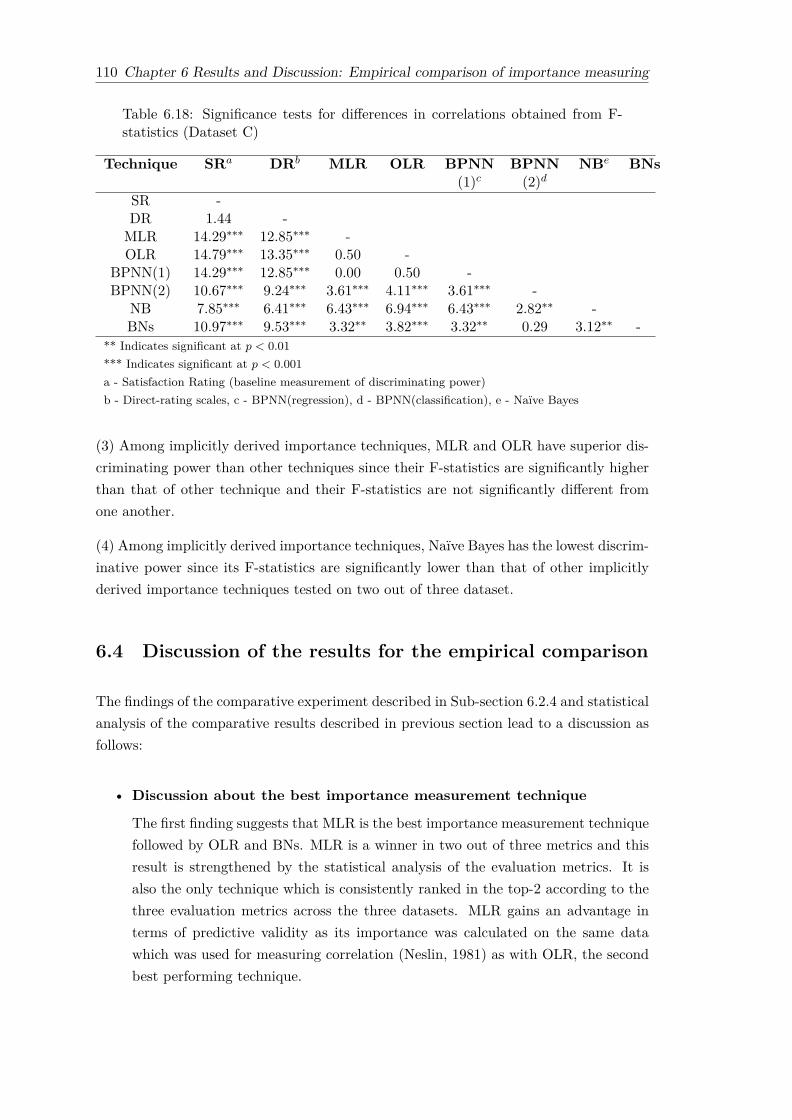
110 Chapter 6 Results and Discussion: Empirical comparison of importance measuring
Table 6.18: Significance tests for differences in correlations obtained from F-statistics (Dataset C)
Technique SRa DRb MLR OLR BPNN BPNN NBe BNs(1)c (2)d
SR -DR 1.44 -MLR 14.29∗∗∗ 12.85∗∗∗ -OLR 14.79∗∗∗ 13.35∗∗∗ 0.50 -
BPNN(1) 14.29∗∗∗ 12.85∗∗∗ 0.00 0.50 -BPNN(2) 10.67∗∗∗ 9.24∗∗∗ 3.61∗∗∗ 4.11∗∗∗ 3.61∗∗∗ -
NB 7.85∗∗∗ 6.41∗∗∗ 6.43∗∗∗ 6.94∗∗∗ 6.43∗∗∗ 2.82∗∗ -BNs 10.97∗∗∗ 9.53∗∗∗ 3.32∗∗ 3.82∗∗∗ 3.32∗∗ 0.29 3.12∗∗ -
** Indicates significant at p < 0.01
*** Indicates significant at p < 0.001
a - Satisfaction Rating (baseline measurement of discriminating power)b - Direct-rating scales, c - BPNN(regression), d - BPNN(classification), e - Naïve Bayes
(3) Among implicitly derived importance techniques, MLR and OLR have superior dis-criminating power than other techniques since their F-statistics are significantly higherthan that of other technique and their F-statistics are not significantly different fromone another.
(4) Among implicitly derived importance techniques, Naïve Bayes has the lowest discrim-inative power since its F-statistics are significantly lower than that of other implicitlyderived importance techniques tested on two out of three dataset.
6.4 Discussion of the results for the empirical comparison
The findings of the comparative experiment described in Sub-section 6.2.4 and statisticalanalysis of the comparative results described in previous section lead to a discussion asfollows:
• Discussion about the best importance measurement technique
The first finding suggests that MLR is the best importance measurement techniquefollowed by OLR and BNs. MLR is a winner in two out of three metrics and thisresult is strengthened by the statistical analysis of the evaluation metrics. It isalso the only technique which is consistently ranked in the top-2 according to thethree evaluation metrics across the three datasets. MLR gains an advantage interms of predictive validity as its importance was calculated on the same datawhich was used for measuring correlation (Neslin, 1981) as with OLR, the secondbest performing technique.

Chapter 6 Results and Discussion: Empirical comparison of importance measuring 111
OLR has high convergent validity with MLR. Hence, the evaluation result of theirimportance is slightly similar to each other. This is confirmed by the statistical testof differences of their results. OLR has the best discriminative power technique.However the difference is not statistically significantly different from MLR, thesecond best discriminative power of the technique, across the three datasets. Onthe other way round, the predictive validity of OLR is not statistically significantlylower than that of MLR in two out of the three datasets. The major difference ofevaluation results between MLR and OLR is the diagnosticity power measured onDataset C.
Despite the fact that both MLR and OLR are superior to the other techniques interms of the three evaluation metrics, they produced negative coefficients in thefirst two datasets as shown in Table 5.9 and Table 5.10. Such negative coefficientsresult in uninterpretable importance measures (Gustafsson and Johnson, 2004).Since they indicate that the customer satisfaction is decrease as the attribute’sperformance is increase, which contradicts to an expectation of basic IPA studiesthat the customer satisfaction should increase as the attribute’s performance is in-crease (Pokryshevskaya and Antipov, 2014). In another word, an attribute with agood performance should positively influent customer satisfaction, therefore, posi-tive importance measures are strongly and theoretically expected. In considerationof the uninterpretable importance measures caused by the negative coefficients, allnegative coefficients obtained from MLR and OLR in this study are set to zero ac-cording to the approach suggested by previous comparative studies of importancemeasures (Gustafsson and Johnson, 2004; Pokryshevskaya and Antipov, 2014).
The problem of negative regression coefficients may stem from the presence ofmulticollinearity among attributes. As Greene (2003) [p.57] suggested that mul-ticollinearity in the regression method may cause the changes in the signs of co-efficients (e.g. switches from positive to negative) that seem theoretically ques-tionable. In this study, the presence of multicollinearity in the three datasets waschecked by inspecting the variance inflation factor (VIF) statistic of each attributein each dataset. The VIFs of all attributes in datasets (Appendix C) showed therewas the presence of multicollinearity (VIF > 1) however none of VIFs exceeds 10which indicate the sign of serious multicollinearity requiring correction.
To avoid the issue of uninterpretable importance measures, a low proportion ofnegative coefficients among attributes are expected (Pokryshevskaya and Antipov,2014). In another word, MLR and OLR would not recommend to use in measuringimportance if they produced a high proportion of negative measures. Recall thatthere are 1/6 and 2/13 of negative coefficients obtained from MLR and OLR indataset A and B (Table 5.9-5.10). These numbers indicate a low proportion ofnegative measures hence, the MLR and OLR are remained preferable choices touse in measuring importance of this study.

112 Chapter 6 Results and Discussion: Empirical comparison of importance measuring
Among the top-3 importance measurement techniques, BNs is the only techniquethat is not prone to produce negative or uninterpretable importance measures.This is preferable in the context of most satisfaction studies (Pokryshevskaya andAntipov, 2014). Although, BNs has a low predictive validity which is about thesame that of the baseline measurement. It is consistently ranked in the top-3 ofdiagnosticity power techniques and it is also the third best discriminate powertechnique.
The fact that the BNs is not a dominant importance measurement technique acrossthree evaluation metrics is somewhat disappointing. Since all implicitly derivedimportance techniques measure the importance on the basis relationship of per-formance and the overall customer satisfaction. It is expected that the better themodel to discover the relationship of performance and the overall customer sat-isfaction, the better the estimates of derived importance will be. Regarding themodel accuracy shown in Table 5.6 - 5.8, BNs yields the top-2 best model accuracymeasured by RMSE in the training and testing mode across the three datasets.Also, RMSE values of BNs are much lower than that of MLR.
The primary implication of this finding is that for the choice of technique to be usedpractically for creating IPA matrix in case there are no uninterpretable importancemeasures, for example- dataset C, MLR and OLR are the recommended techniques.Otherwise, BNs is a preferable technique.
• Discussion about self-stated importance vs implicitly derived impor-tance
The second finding that direct-rating scales is the worst importance measurementtechnique, indicates that the implicitly derived importance techniques are superiorat measuring importance to the self-stated importance using direct-rating scalesas most implicitly derived importance techniques yielded better results than thatof direct-rating scales in three evaluation metrics. Although the differences of theevaluation metrics are not significant different for all three datasets.
On the one hand, this finding supports the claim made by Neslin (1981) that theregression as the implicitly derived importance technique is superior to self-statedimportance technique in terms of predictive ability. However on the other hand,this finding contradicts the research finding of Bacon (2003) and Gustafsson andJohnson (2004) which claimed that the self-stated importance technique is betterthan at least one implicitly derived importance technique - MLR.
Additionally, when comparing the predictive validity and discriminative power ofself-stated importance and implicitly derived importance with the baseline mea-surement, it shows that importance measured by both types of techniques improvepredictive validity and discriminative power of the baseline technique which con-siders each attribute is equally important when determining overall satisfaction.However the latter yields better improves of the two metrics than the former.

Chapter 6 Results and Discussion: Empirical comparison of importance measuring 113
This minor finding confirms the superiority of implicitly derived importance overthe self-stated importance and shows the merit of the importance measured bythe techniques. In other words it shows that importance measured by the tech-niques is a valid predictor of overall customer satisfaction and a valid indicatorfor identifying key attributes that drive customer satisfaction as importance mea-sures improve predictive validity and discriminative power when computed solelyon performance.
It can be simply said that the presence of importance yielded a better predictivevalidity and discriminative power than when it was omitted (baseline measure-ment) and the importance measured by implicitly derived techniques even yieldedbetter results than importance measured by self-stated technique. This result isconfirmed by the statistical test of predictive validity and discriminative power ofat least two out of the three datasets.
• Discussion about statistically inferred importance vs data mining im-plicitly derived importance
The third finding suggests that Naïve Bayes is the second worst importance mea-surement technique and the worst implicitly derived importance technique basedon the average rank of three evaluation metrics, and it ranked after BPNN(regression)and BPNN(classification). This primarily suggests that Naïve Bayes may not asuitable technique to be used for measuring importance.
Although, using Naïve Bayes to measure importance does little to improve predic-tive ability from using customer self-stated importance measure, its major short-coming is an ability to discriminate importance among attributes as evaluatedby discrimination power and diagnosticity power. This is also a drawback of thecustomer self-stated technique. The reason for this outcome can be gleaned fromthe assumption of Naïve Bayes that all attributes contribute equally and inde-pendently to the class or the overall customer satisfaction in this context (Moranet al., 2009). Thereby the importance derived from the Naïve Bayes model in oneattribute is not much different than the others and there is a small range of im-portance measures between the most important attribute and the least importantattribute.
Recall that the derived importance measurement techniques can be further cat-egorized into two groups which are statistically inferred importance and datamining implicitly derived importance. This finding also suggests that the sta-tistically inferred importance techniques which are MLR and OLR, are superiorto all data mining implicitly derived importance techniques including BNs andBPNN(regression/classification), Naïve Bayes since, these data mining implicitlyderived importance techniques are ranked from third to sixth among the impor-tance measurement techniques respectively.

114 Chapter 6 Results and Discussion: Empirical comparison of importance measuring
The finding that MLR is superior to both types of BPNN differ from Deng et al.(2008a) and Krešić et al. (2013) studies which reported that BPNN yielded abetter improvement in estimating importance compared to MLR. However, theseprevious studies did not compare importance estimated by MLR and BPNN againstevaluation metrics. These two previous studies compared only the model qualityin learning pattern of data measured by Root Mean Squared Error (RMSE) andgoodness-of-fit of the model between MLR and BPNN and concluded in favour ofBPNN.
In conclusion, the third finding raised a case that the simple techniques - MLRand OLR work best. As MLR is an easy-to-use technique which makes it be afavourable choice to be used practically in the real world so as to OLR. While, theuse of data mining implicitly derived importance techniques such as BPNN andBNs required a user who has good background knowledge about the techniques tospecify several training parameters in order to get an accurate result. Additionally,importance can be obtained straightforwardly from the outcome of MLR and OLRwhereas further steps are needed to estimate importance from the outcome of alldata mining implicitly derived importance techniques.
• Discussion about analytical techniques and type of dependent variable
Recall that the techniques for measuring importance fitted the model by consid-ering the dependent variable which is overall satisfaction in three different datatypes: quantitative (interval scales), categorical, ordinal categorical.
Theoretically, overall satisfaction measured in Likert scales is ordinal categoricalvariable (Jamieson et al., 2004). Therefore, it is expected that OLR, the techniquethat fits a model by treating the dependent variable as ordinal categorical data,should be the best importance measure technique. However, the first finding re-vealed that OLR is the second best importance measure technique and it is rankedafter MLR that fits a model by treating the dependent variable as quantitative.
Although MLR requires the dependent variable to be quantitative continuouswhich is not compatible with the ordinal nature of the overall satisfaction (Chenand Hughes, 2004), it is the commonly used technique for indirectly measuringimportance (Lai and Hitchcock, 2015). Additionally, there has been a long con-troversy about treating Likert-derived data as quantitative (Jamieson et al., 2004).The first finding of this study supports the use of MLR and reveals that treatingLikert-derived data as quantitative does not affect the importance estimation. Itcan be simply said that considering level order of dependent variable does not yielda better improvement of importance estimation.
In addition, the fourth finding demonstrates that the importance estimation is notdirectly affected by different data types of the dependent variable required by eachtechnique as it reports that BPNN(regression) outperforms BPNN(classification)at measuring importance. While it is expected that BPNN(classification) should

Chapter 6 Results and Discussion: Empirical comparison of importance measuring 115
be able to produce better importance measures than BPNN(regression) since,BPNN(classification) fits a model by treating the dependent variable as categori-cal which is more compatible with the nature of the overall satisfaction than theBPNN(regression) that fits a model by treating the dependent variable as quanti-tative.
In accordance with the implications drawn from the first and the fourth findings,comparative results of BNs and Naïve Bayes show that there is really a differentranked order between these two techniques which are 3rd and 6th respectivelyalthough both of them fit a model by treating the dependent variable as categorical.
Furthermore, different data types of the dependent variable required by each tech-nique does not directly affect the convergent validity among techniques. For exam-ple, MLR and OLR treat the dependent variable as different data types but thereis a high convergent validity between them. In contrast, both Naïve Bayes andBNs treat the dependent variable as categorical but there is a lack of convergentvalidity between them.
6.5 Summary
This chapter reports results of the comparative experiment which was conducted in theprevious chapter to help answer the first research question. The empirical comparisonresults demonstrate that MLR is the best importance measure technique whereas direct-rating scales is the worst importance measure technique in terms of the three evaluationmetrics. Hence, the author supports the use of implicitly derived importance measuresinstead of self-stated importance measures. The use of an implicitly derived importancetechnique not only provides reliable importance measures but also shortens the survey’slength by removing questions about importance rating.
OLR is the second best importance measures technique which has high convergent va-lidity with MLR. These two techniques are further classified as the statistically inferredimportance measure whereas BNs, BPNN(regression/classification), and Naïve Bayesthat ranked the third to sixth best importance measures are classified as data miningimplicitly derived importance techniques. Thus, it can be concluded that the statisti-cally inferred importance techniques are superior to the data mining implicitly derivedimportance techniques.
The statistical analysis of comparative results also confirmed the fact that MLR is thebest importance measures technique since, the predictive validity of MLR is significantlyhigher than most techniques tested on two out of three datasets and discriminating powerof MLR is significantly higher than that of other techniques except OLR tested acrossthe three datasets. For the diagnosticity metric, diagnosticity of MLR is only signifi-cantly higher than that of other techniques except OLR in one dataset as significantly

116 Chapter 6 Results and Discussion: Empirical comparison of importance measuring
differences between two values of diagnosticity were difficult to detect in a small dataset.However, the diagnosticity of MLR is significantly different from that of direct-ratingscales in two out of the three datasets.
Although MLR produced some negative regression coefficients, the proportion of themis considerably low. This drawback of MLR is not a case to be concerned and it is atrade-off for other advantages of MLR as stated in previous paragraph. Based on thesefindings, MLR is chosen to measure importance in the IPA based SWOT analysis frame-work. As MLR is an easy-to-use technique, the use of MLR facilitates the frameworkto be practically used in the real world. The details of the IPA based SWOT analysisframework are described in the next chapter.

Chapter 7
IPA based SWOT analysis
Based on the results of the previous chapter, a technique for measuring importance wasidentified and applied in a methodological framework for developing SWOT analysisfrom IPA results, called Importance-Performance Analysis based SWOT analysis (IPAbased SWOT analysis). This framework serves as an outline of the main steps to becompleted in order to obtain an organisation’s SWOT from survey data.
This chapter introduces an IPA based SWOT analysis starting by describing its back-ground in 7.1. Then, a framework of applying IPA for SWOT analysis is described inSection 7.2.
7.1 Background of IPA based SWOT analysis
Recall that there are three issues related to the development of the IPA based SWOTanalysis: (1) selecting a technique for measuring importance, (2) identifying opportu-nities and threats from a customer satisfaction survey and (3) evaluation of IPA basedSWOT analysis. This chapter focuses on addressing the second issue, while the firstissue has already been addressed by conducting the empirical comparison of varioustechniques for measuring importance in which the methodology and results were ex-plained in Chapter 5 and 6 respectively.
The second issue is associated with the second research question “How can IPA be appliedto develop a SWOT analysis based on a customer satisfaction survey?” To address thisresearch question, the library research was conducted to review the connection betweenIPA and SWOT analysis and specify the possible way to acquire all SWOT aspectsfrom the IPA results, known as IPA matrix. The review of literature indicated thecorrespondence between IPA and SWOT analysis in two different ways. Several IPApapers directly interpret each quadrant of the IPA as each aspect of SWOT shown inFigure 7.1 (Duke and Mount, 1996; Kim and Oh, 2001; Luo et al., 2010).
117
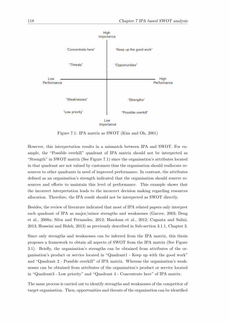
118 Chapter 7 IPA based SWOT analysis
Figure 7.1: IPA matrix as SWOT (Kim and Oh, 2001)
However, this interpretation results in a mismatch between IPA and SWOT. For ex-ample, the “Possible overkill” quadrant of IPA matrix should not be interpreted as“Strength” in SWOT matrix (See Figure 7.1) since the organisation’s attributes locatedin that quadrant are not valued by customers thus the organisation should reallocate re-sources to other quadrants in need of improved performance. In contrast, the attributesdefined as an organisation’s strength indicated that the organisation should reserve re-sources and efforts to maintain this level of performance. This example shows thatthe incorrect interpretation leads to the incorrect decision making regarding resourcesallocation. Therefore, the IPA result should not be interpreted as SWOT directly.
Besides, the review of literature indicated that most of IPA related papers only interpreteach quadrant of IPA as major/minor strengths and weaknesses (Garver, 2003; Denget al., 2008a; Silva and Fernandes, 2012; Hasoloan et al., 2012; Cugnata and Salini,2013; Hosseini and Bideh, 2013) as previously described in Sub-section 3.1.1, Chapter 3.
Since only strengths and weaknesses can be inferred from the IPA matrix, this thesisproposes a framework to obtain all aspects of SWOT from the IPA matrix (See Figure3.1). Briefly, the organisation’s strengths can be obtained from attributes of the or-ganisation’s product or service located in “Quadrant1 - Keep up with the good work”and “Quadrant 2 - Possible overkill” of IPA matrix. Whereas the organisation’s weak-nesses can be obtained from attributes of the organisation’s product or service locatedin “Quadrant3 - Low priority” and “Quadrant 4 - Concentrate here” of IPA matrix.
The same process is carried out to identify strengths and weaknesses of the competitor oftarget organisation. Then, opportunities and threats of the organisation can be identified

Chapter 7 IPA based SWOT analysis 119
by comparing strengths and weaknesses of organisation with that of its competitor basedon the ideas of Pai et al. (2013) which stated that “the strengths of competitor become thethreats of the organisation and the weaknesses of competitors can become the opportunitiesof the organisation”.
7.2 IPA based SWOT analysis Framework
Main idea of this framework is to use IPA to analyse survey data of the organisation andits competitors, then the organisation’s SWOT factor is derived from the IPA matrix asshown in Figure 7.2. The IPA based SWOT analysis comprises four steps:
Figure 7.2: Proposed framework for applying IPA to SWOT analysis
Step 1: Undertake a customer satisfaction survey. First and foremost, attributesof an organisation’s product or service are identified based on a thorough literaturereview in each application area or by interviews (Martilla and James, 1977; Skoket al., 2001; Levenburg and Magal, 2005). Then, a survey is developed regardingthe identified attributes of an organisation’s product or service.

120 Chapter 7 IPA based SWOT analysis
Generally, a survey that is suitable for applying IPA consists of an assessment ofrespondents’ satisfaction for an organisation’s product or service which is measuredby a Likert scale with either five or seven levels (Lai and Hitchcock, 2015). Inaddition, the survey should contain an assessment of overall satisfaction on theLikert scale. Two surveys using the same set of questions are required in thisstudy. The first survey focuses on the service quality of the target organisation,while the second survey concentrates on the service quality of the organisation’scompetitor.
Step 2: Conduct an IPA on the customer survey. After the surveys are admin-istered to customers of a target organisation and customers of an organisation’scompetitor, the customer survey data is processed to compute importance andperformance for an individual attribute of an organisation’s product or service.Procedures associated to this step are shown in Figure 7.3, and discussed below.
Figure 7.3: Steps for conducting IPA of customer survey data
• Calculate importance. Through this work, attributes’ importance is derivedfrom survey responses based on the relationships between attributes’ perfor-mance and overall satisfaction instead of asking customers to rate the im-portance. Specifically, MLR is chosen to analyse the survey data and com-pute attribute’ importance as MLR is the best implicitly derived importancemethod with regard to an empirical comparison results described in Chap-ter 6.

Chapter 7 IPA based SWOT analysis 121
MLR is applied to the survey data to create a model for discovering the rela-tionship between the attributes’ performance of the product or services andoverall satisfaction which reveals the attributes that influence the overall sat-isfaction. All attributes’ performance are set as independent variables andoverall satisfaction is set as dependent variable.
The regression coefficients obtained from the MLR model can be referred toas implicit importance since the regression coefficient generally indicates howmuch a one unit increase in the independent variable results in an increaseor decrease in the dependent variable with all other variables held constant(Nathans et al., 2012).
• Calculate performance. The performance for each attribute of an organisa-tion’s products or services is computed by averaging performance ratings fromall respondents to the questionnaire which is called “actual performance”.
• Construct the IPA Matrix. The grand mean of attributes’ importance andgrand mean of attributes’ performance are calculated, and then used to dividethe IPA matrix into four quadrants. Finally, all attributes’ importance andattributes’ performance calculated in previous procedures are plotted on thex-axis and y-axis of IPA matrix respectively.
Step 3: Identify strengths and weaknesses through the IPA matrix. With re-gard to the IPA matrix produced in Step 2, an organisation’s attributes located inQuadrant 1 and Quadrant 2 are identified as strengths as they have high perfor-mance, whereas an organisation’s attributes located in Quadrant 3 and Quadrant4 are identified as weaknesses as they are having low performance. Based onthe same principle, strengths and weaknesses of the organisation’s competitor areidentified from the IPA matrix of competitor.
Step 4: Identify opportunities and threats through IPA matrix. By comparingthe attributes of an organisation and its competitor that were previously labelledas strength and weakness, opportunities and threats of the organisation can beidentified based on the ideas of Pai et al. Pai et al. (2013) which stated that “thestrengths of competitor become the threats of the organisation and the weaknessesof competitors can become the opportunities of the organisation”.
A summary of the identification for all aspects of SWOT and their managerialimplication is presented in Table 7.1 and described as follows:
Strength (S). Attribute is labelled as an organisation’s strength, since it is iden-tified as a strength of an organisation and its competitor. This means both atarget organisation and its competitor are performing well at providing this
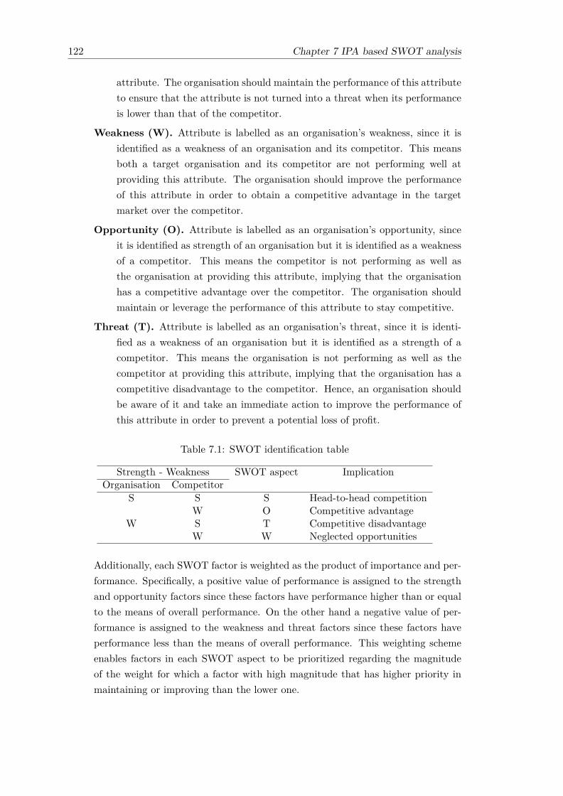
122 Chapter 7 IPA based SWOT analysis
attribute. The organisation should maintain the performance of this attributeto ensure that the attribute is not turned into a threat when its performanceis lower than that of the competitor.
Weakness (W). Attribute is labelled as an organisation’s weakness, since it isidentified as a weakness of an organisation and its competitor. This meansboth a target organisation and its competitor are not performing well atproviding this attribute. The organisation should improve the performanceof this attribute in order to obtain a competitive advantage in the targetmarket over the competitor.
Opportunity (O). Attribute is labelled as an organisation’s opportunity, sinceit is identified as strength of an organisation but it is identified as a weaknessof a competitor. This means the competitor is not performing as well asthe organisation at providing this attribute, implying that the organisationhas a competitive advantage over the competitor. The organisation shouldmaintain or leverage the performance of this attribute to stay competitive.
Threat (T). Attribute is labelled as an organisation’s threat, since it is identi-fied as a weakness of an organisation but it is identified as a strength of acompetitor. This means the organisation is not performing as well as thecompetitor at providing this attribute, implying that the organisation has acompetitive disadvantage to the competitor. Hence, an organisation shouldbe aware of it and take an immediate action to improve the performance ofthis attribute in order to prevent a potential loss of profit.
Table 7.1: SWOT identification table
Strength - Weakness SWOT aspect ImplicationOrganisation Competitor
S S S Head-to-head competitionW O Competitive advantage
W S T Competitive disadvantageW W Neglected opportunities
Additionally, each SWOT factor is weighted as the product of importance and per-formance. Specifically, a positive value of performance is assigned to the strengthand opportunity factors since these factors have performance higher than or equalto the means of overall performance. On the other hand a negative value of per-formance is assigned to the weakness and threat factors since these factors haveperformance less than the means of overall performance. This weighting schemeenables factors in each SWOT aspect to be prioritized regarding the magnitudeof the weight for which a factor with high magnitude that has higher priority inmaintaining or improving than the lower one.

Chapter 7 IPA based SWOT analysis 123
7.3 Summary
This chapter describes the IPA based SWOT analysis framework which offers a system-atic way to analyse customer satisfaction surveys by using IPA in identifying SWOT, soas to answer the second research question. Through the steps explained in the proposedframework an organisation’s SWOT can be obtained from survey data.
The key steps of the IPA based SWOT analysis are the IPA matrix construction in whicha customer satisfaction survey is analysed to calculate the importance and performance,and SWOT factors identification based on the IPA matrix. Specifically, strengths andweaknesses are identified through an IPA matrix of the organisation, while opportunitiesand threats are obtained by comparing the IPA matrix of an organisation with that ofits competitor.
By using IPA based SWOT analysis, the generated SWOT factors are not only measur-able regarding the importance and performance but also meaningful as they are identifiedbased on customers’ points of view. A measurable SWOT factor enables an organisationto prioritize SWOT factors in creating an action plan while a customer oriented SWOTfactor guarantees that the capabilities perceived by an organisation are recognized andvalued by the customers. This facilitates an organisation to efficiently formulate strategicplanning for maintaining or enhancing customer satisfaction, thereby gaining a compet-itive advantage.
To demonstrate the proficiency of the IPA based SWOT analysis in the real-world situa-tion, the case study of Higher Education Institutions (HEIs) in Thailand are conductedand then the SWOT of the case study are evaluated. The details of case study and IPAbased SWOT evaluation methodology are described in the next chapter.


Chapter 8
IPA based SWOT analysis:Evaluation Methodology
To demonstrate and evaluate the IPA based SWOT analysis which was introduced in theprevious chapter, the case study of Higher Education Institutions (HEIs) in Thailand wasconducted and is explained in this chapter. Three surveys were conducted as part of thecase study following the survey research method. The first one is a student satisfactionsurvey which was conducted for the purpose of demonstrating how IPA based SWOTanalysis can be used to generate SWOT. The last two surveys are staff evaluation ofSWOT survey and experienced users of SWOT survey which were conducted for thepurpose of evaluation of IPA based SWOT analysis so as to answer the third researchquestion “How good is the outcome of IPA based SWOT analysis?”
The aim of this chapter is to describe the methodologies related to the case study includ-ing the survey research method for conducting the three surveys and the implementationof IPA based SWOT analysis on student satisfaction survey. This chapter is organisedas follows: Section 8.1 provides background of the organisations involved in the casestudy. Section 8.2 describes the methodology for conducting student satisfaction sur-vey. Section 8.3 illustrates the IPA based SWOT analysis framework implemented onthe student satisfaction survey. Section 8.4 and Section 8.5 describes the methodologyfor conducting the staff evaluation of SWOT survey and experienced users of SWOTsurvey respectively.
125

126 Chapter 8 IPA based SWOT analysis: Evaluation Methodology
8.1 Background of the case study
The department of Computer Engineering at Kamphaeng Saen campus (CPE-KU-KPS,henceforth KPS), Kasetsart University was selected as the case study of HEIs in Thai-land, and its competitor is the department of Computer Engineering at Bangkhen Cam-pus (CPE-KU-BKN, henceforth BKN).
KPS, the selected target organisation, was established in 2006 and located in the secondcampus of Kasetsart University. KPS’s mission is to produce graduates in the field ofcomputer engineering with quality, integrity and ethics, as well as support the coun-try with know-how in the field of information technology. At present, the KPS stillfirmly commits to the mission and continuously improves teaching quality, research,and academic service to produce specialized graduates.
KPS was chosen as a target organisation because this department needed an improve-ment to be in the Thailand top 10 for computer engineering. However, KPS still hasno concrete future plan since the department’s future plan was formulated based on animprecise SWOT list in which some ideas were raised from personal attitudes in thebrainstorming with no supporting evidence or documents. The issues were observedbased on the experience of the author who is one of the staff members in KPS.
BKN, the selected competitor, was established in 1989 and located on the main campusof Kasetsart University in the state capital. The BKN is in the Thailand top threefor computer engineering. It has academic strengths and expertise in computer engi-neering which is guaranteed by both national and international awards, for instance,Skuba - a Small size robot soccer team- were the world champion team in RoboCup forthe fourth consecutive year (2009-2012), an award-winning entertainment program ofNational Software Contest (NSC 2012).
BKN was chosen as a competitor of KPS because it has academic strengths and expertisein computer engineering. BKN is also ranked in the first place of the top computerengineering department in Thailand regarding the central university admissions test20141, which guarantee that BKN has renowned teaching and research in computerengineering.
As with other universities, these two departments of Kasetsart University generallyconduct student satisfaction surveys about the aspects of the department to assess theperformance of the department. Data from these surveys can be further analysed toproduce SWOT of KPS by applying the IPA based SWOT analysis framework whichwill provide useful information for formulating a concrete future plan for the department.
Through the case study, SWOT of KPS was generated regarding the IPA based SWOTanalysis framework which was implemented on the student satisfaction surveys response
1www.cuas.or.th/document/57D_stat_rpass_web.pdf

Chapter 8 IPA based SWOT analysis: Evaluation Methodology 127
by undergraduate students of KPS and BKN. Then, the SWOT of KPS was evaluatedby using the staff evaluation of SWOT survey and experienced users of SWOT survey.Detail about the three surveys and implementation of IPA based SWOT analysis aredescribed in the following sections.
8.2 Methodology for conducting student satisfaction sur-vey
Regarding the first step of an IPA based SWOT framework (see section 7.2), a stu-dent satisfaction survey was undertaken in KPS and BKN. The results of the studentsatisfaction survey will be used as inputs of IPA. It is essential that the survey of theorganisation and its competitor use the same questionnaire so that the IPA matrix ofthe competitor can be combined with the IPA matrix of the target organisation whichfulfils all aspects of SWOT. Following the survey research method, tasks for undertakingstudent satisfaction survey are described in the following sub-sections.
8.2.1 Questionnaire design
The questionnaire used was divided into two sections. In the first section, students wereasked to provide their perceived performance responses towards six departments’serviceattributes as well as the overall satisfaction. Subsequently, students were asked to pro-vide their importance responses for each of the same attributes. This section containedclosed-response questions, on a five-Likert scale. The second section refers to the de-mographic data of students such as academic year, gender and study program (regular/special).
The six attributes that were selected based on a list of attributes defined in previousstudies of student satisfaction (Siskos and Grigoroudis, 2002; Silva and Fernandes, 2011;Grebennikov and Shah, 2013) are shown below.
1. Academic Personnel: Teaching ability, Subject expertise, Friendliness of teachingstaff;
2. Teaching and Learning: Lecture materials, e-learning resources, Fair assessment,Class size, and Teaching facilities and classroom condition;
3. Administration: Knowledge of rules and procedures of staff members, Friendlinessof staff members, Ability of the staff members to provide services in a timelymanner;
4. Computer Facilities: Quality and Availability of computer facilities, Availability ofInternet access, and Availability of printing and photocopying facilities;
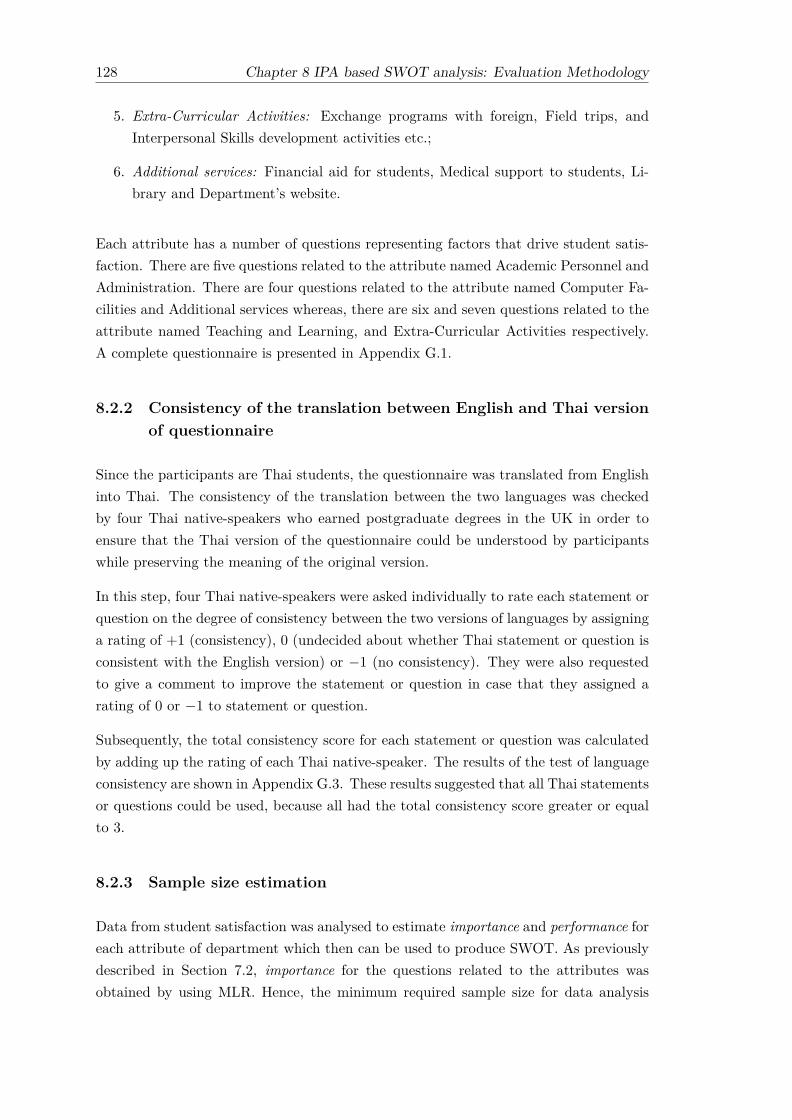
128 Chapter 8 IPA based SWOT analysis: Evaluation Methodology
5. Extra-Curricular Activities: Exchange programs with foreign, Field trips, andInterpersonal Skills development activities etc.;
6. Additional services: Financial aid for students, Medical support to students, Li-brary and Department’s website.
Each attribute has a number of questions representing factors that drive student satis-faction. There are five questions related to the attribute named Academic Personnel andAdministration. There are four questions related to the attribute named Computer Fa-cilities and Additional services whereas, there are six and seven questions related to theattribute named Teaching and Learning, and Extra-Curricular Activities respectively.A complete questionnaire is presented in Appendix G.1.
8.2.2 Consistency of the translation between English and Thai versionof questionnaire
Since the participants are Thai students, the questionnaire was translated from Englishinto Thai. The consistency of the translation between the two languages was checkedby four Thai native-speakers who earned postgraduate degrees in the UK in order toensure that the Thai version of the questionnaire could be understood by participantswhile preserving the meaning of the original version.
In this step, four Thai native-speakers were asked individually to rate each statement orquestion on the degree of consistency between the two versions of languages by assigninga rating of +1 (consistency), 0 (undecided about whether Thai statement or question isconsistent with the English version) or −1 (no consistency). They were also requestedto give a comment to improve the statement or question in case that they assigned arating of 0 or −1 to statement or question.
Subsequently, the total consistency score for each statement or question was calculatedby adding up the rating of each Thai native-speaker. The results of the test of languageconsistency are shown in Appendix G.3. These results suggested that all Thai statementsor questions could be used, because all had the total consistency score greater or equalto 3.
8.2.3 Sample size estimation
Data from student satisfaction was analysed to estimate importance and performance foreach attribute of department which then can be used to produce SWOT. As previouslydescribed in Section 7.2, importance for the questions related to the attributes wasobtained by using MLR. Hence, the minimum required sample size for data analysis
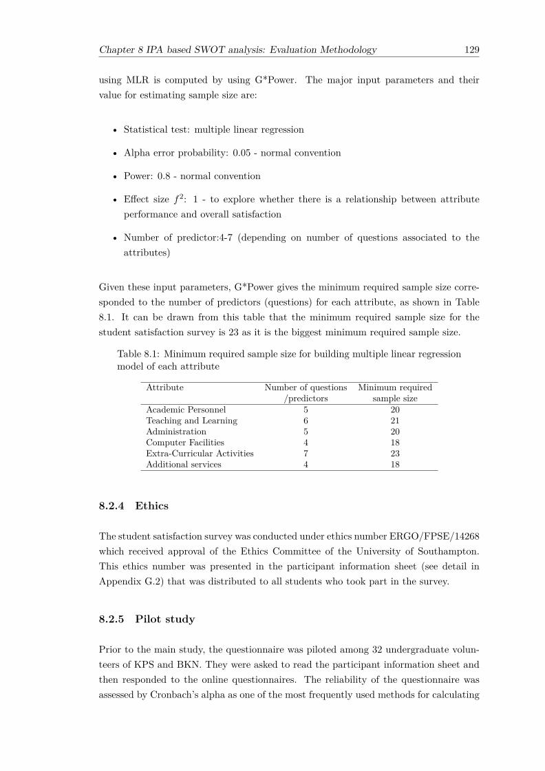
Chapter 8 IPA based SWOT analysis: Evaluation Methodology 129
using MLR is computed by using G*Power. The major input parameters and theirvalue for estimating sample size are:
• Statistical test: multiple linear regression
• Alpha error probability: 0.05 - normal convention
• Power: 0.8 - normal convention
• Effect size f2: 1 - to explore whether there is a relationship between attributeperformance and overall satisfaction
• Number of predictor:4-7 (depending on number of questions associated to theattributes)
Given these input parameters, G*Power gives the minimum required sample size corre-sponded to the number of predictors (questions) for each attribute, as shown in Table8.1. It can be drawn from this table that the minimum required sample size for thestudent satisfaction survey is 23 as it is the biggest minimum required sample size.
Table 8.1: Minimum required sample size for building multiple linear regressionmodel of each attribute
Attribute Number of questions Minimum required/predictors sample size
Academic Personnel 5 20Teaching and Learning 6 21Administration 5 20Computer Facilities 4 18Extra-Curricular Activities 7 23Additional services 4 18
8.2.4 Ethics
The student satisfaction survey was conducted under ethics number ERGO/FPSE/14268which received approval of the Ethics Committee of the University of Southampton.This ethics number was presented in the participant information sheet (see detail inAppendix G.2) that was distributed to all students who took part in the survey.
8.2.5 Pilot study
Prior to the main study, the questionnaire was piloted among 32 undergraduate volun-teers of KPS and BKN. They were asked to read the participant information sheet andthen responded to the online questionnaires. The reliability of the questionnaire wasassessed by Cronbach’s alpha as one of the most frequently used methods for calculating

130 Chapter 8 IPA based SWOT analysis: Evaluation Methodology
internal consistency (Saunders et al., 2009). As a rule of thumb Cronbach’s alpha valuegreater than 0.7 is considered reliable (De Vaus, 2002b). The reliability values for eachattribute’s performance is shown in Table 8.2. The Cronbach’s alpha for each attributeof the department ranged from 0.86 to 0.97 as shown in Table 8.2. The Cronbach’s alphaof all groups was greater than 0.70 thus it can be concluded that the questionnaire hasgood internal consistency.
Table 8.2: List of attributes used in the case study and Cronbach’s alpha
Attribute Question/Factor Cronbach’s alphaAcademic Teaching ability of teaching staff 0.86Personnel Subject expertise of teaching staff
(Teacher1-5) Friendliness of teaching staffAvailability of teaching staffAdvice and support in learning
Teaching Lecture materials 0.92and Learning e-learning resources(Teaching1-6) Assessments (clarity and timely feedback)
Class sizeAccurate and up-to-date unit contentTeaching facilities and classroom condition
Administration Knowledge of rules and procedures of staff 0.97(Admin1-5) Knowledge of the information about courses, ex-
ams, activities of staffInterest in solving student’s problems by staffFriendliness of staffAbility of staff to provide services in a timely manner
Computer Quality of computer facilities 0.95Facilities Availability of computer facilities
(CompFac1-4) Availability of internet accessAvailability of printing and photocopying facilities
Extra-Curricular Cultural exchange programs with foreign country 0.97Activities Field trips
(xActivity1-7) Moral development activitiesHealth development activitiesInterpersonal skills development activitiesPersonal learning and thinking skills development activitiesSocial volunteer activities
Additional Services Financial aid for students 0.96(AddService1-4) Medical support to students
Department websiteLibrary
8.2.6 Data collection
KPS and BKN students were asked face to face to take part in the survey by the repre-sentative of the researcher in their classroom during April and May of 2014, in the second

Chapter 8 IPA based SWOT analysis: Evaluation Methodology 131
semester of the 2014/2015 academic year. They were asked to read the participant in-formation sheet and then responded to the online questionnaires available at: https://www.isurvey.soton.ac.uk/15462 (KPS version) and https://www.isurvey.soton.ac.uk/ 15415(BKN version). The printed versions are shown in Appendix G.1.
A total of 155 and 43 valid questionnaires were collected for analysis from KPS and BKNrespectively. Note that the sample size of both department were greater than 23 which isthe minimum required sample size for data analysis using MLR computed by G*Power(see sub-section 8.2.3). Data characteristics of the samples from the two departmentsare shown in Table 8.3 and 8.4.
Table 8.3: General characteristics of sample CPE-KU-KPS students (N=155)
Characteristics Number Percentage (%)GenderMale 91 58.7Female 60 38.7Missing 4 2.6
Study Level1 22 14.22 78 50.33 30 19.44 22 14.2Other 1 0.6Missing 2 1.3
ProgramRegular 95 61.3Special 58 37.4Missing 2 1.3
Table 8.3 lists general characteristics of sample KPS students who participated in thesurvey. The sample of 155 students comprise of 91 (58.7%) males and 60 (38.7%) females,with four missing entries accounting for the remaining 2.6%. The majority are the secondyear students which is about 50.3% of overall sample. 95 (61.3%) students are studiedin a regular program and 58 (37.4%) students are studied in a special program.
Table 8.4 lists general characteristics of the sample of BKN students who participatedin the survey. The sample of 43 students comprise of 36 (83.7%) males and 6 (14.0%)females, with one missing entry accounting for the remaining 2.3%. The majority are thesecond year students which is about 39.5% of the overall sample. 29 (67.4%) studentsstudied in a regular program and 13 (30.2%) students studied in a special program.

132 Chapter 8 IPA based SWOT analysis: Evaluation Methodology
Table 8.4: General characteristics of sample CPE-KU-BKN students (N=43)
Characteristics Number Percentage (%)GenderMale 36 83.7Female 6 14.0Missing 1 2.3
Study Level1 1 2.32 17 39.53 9 20.94 14 32.6Other 1 2.3Missing 1 2.3
ProgramRegular 29 67.4Special 13 30.2Missing 1 2.3
8.2.7 Data analysis method
The student satisfaction survey data collected through the previous steps was thenprocessed following step 2 - step 4 of IPA based SWOT framework as described inSection 7.2, chapter 7 in order to generate SWOT of KPS. Detail of the implementationof IPA based SWOT analysis on student satisfaction survey is described in the nextsection.
8.3 Implementation of IPA based SWOT analysis
This section describes how the student satisfaction survey was processed following step2 - step 4 of IPA based SWOT framework as described in Section 7.2, chapter 7 in orderto generate SWOT of KPS. Results produced from step 2 - step 4 of IPA based SWOTframework which are IPA matrices, strengths-weaknesses of the two departments, andSWOT of KPS are presented in Section 9.1, Chapter 9.
Regarding the step 2 of IPA based SWOT framework, data from the student satisfactionsurvey of KPS and BKN were analysed to create two IPA matrices. The main taskswithin this step are calculating of importance and performance for individual factorrelated to the attribute of the department, and constructing the IPA matrix.
• Calculate importance. For each attribute, the MLR model was constructed usingSPSS to obtain importance as a regression coefficient. Recall that there were six

Chapter 8 IPA based SWOT analysis: Evaluation Methodology 133
attributes of the department as shown in Table 8.2, hence six regression modelswere constructed corresponding to the number of attributes.
Each model has different set of independent variables which is the performance offactors (or questions) related to the attribute, but it has the same dependent vari-able which is the overall student satisfaction. For example, there were five indepen-dent variables involved in building the regression model of the attribute AcademicPersonnel namely “Teaching ability”, “Subject expertise”, “Friendliness”, “Avail-ability”, and “Advice and support in learning” of teaching staff. All independentvariables related to the six attributes are presented in Table 8.2.
All independent variables associated with attributes were entered into the modelsimultaneously as the forced entry is set for the method of regression. Once theregression models were trained, the importance was measured as the standardizedregression coefficient of the model. Additionally, all importance was expressedas a percentage contribution of factor with the negative importance set to zero,which allows the importance measures of the KPS and BKN to be comparable.This approach has been used in some previous comparative studies of importancemeasures (Gustafsson and Johnson, 2004; Pokryshevskaya and Antipov, 2014).
Lastly, it is important to note that assumptions of MLR (such as normality, mul-ticollinearity) tested on KPS and BKN surveys were checked and found not tobe violated (see Appendix H and Appendix I). Thus, it can be assured that theMLR were properly conducted which results in reliable regression coefficients forimportance obtained from the surveys of the two departments in the case study.
• Calculate performance. For each factor under the six attributes, the performanceof KPS and BKN was calculated as a mean of satisfaction. The performance ofthe KPS and BKN were comparable since the satisfaction of the two departmentswas measured in the same scale of 5.
• Construct the IPA Matrix. The intersection between the x-axis and y-axis togenerate a four-quadrant matrix was calculated as the grand mean of all importanceand all performance of the KPS and BKN. The use of grand means provides a faircomparison between the IPA matrix of both departments. Then, the coordinatesof importance and performance for each factor under the six attributes were plottedto generate complete IPA matrices of the two departments (see Table 9.1).
Regarding the step 3 of the IPA based SWOT framework, the IPA matrix of KPS andBKN were examined to identify strengths and weaknesses of the department. Factorslocated in Quadrant 1 and Quadrant 2 of IPA matrix are identified as strengths as theirperformance is higher than the grand mean of performance, whereas factors locatedin Quadrant 3 and Quadrant 4 of IPA matrix are identified as weaknesses as theirperformance is lower than the grand mean of performance.

134 Chapter 8 IPA based SWOT analysis: Evaluation Methodology
Regarding the step 4 of the IPA based SWOT framework, the opportunities and threatsof KPS were identified by comparing the factors of KPS and BKN that were previouslylabelled as strengths and weaknesses to generate a complete SWOT of KPS (see Ta-ble 9.2). This identification of opportunities and threats was conducted regarding theSWOT identification table presented in Table 7.1. In addition to the label of SWOTaspect, each factor also has the weight attached which was computed as the product ofimportance and performance, allowing the department to do factor prioritization withina SWOT group.
8.4 Methodology for conducting staff evaluation of SWOTsurvey
An IPA based SWOT analysis was completed based on student satisfaction towardservices offered by KPS. The IPA-SWOT of KPS was then evaluated by staff at KPS,the staff all had worked at KPS for at least two years, hence they can be consideredas domain experts. The aim of the evaluation was to answer sub research question 3.1,that is, do staff agree with the analysis. The staff’s level of agreement on the IPA-SWOT of KPS provides face validity of the proposed approach. The evaluation alsoreveals how well the staff recognises organisation’s competences given by their customers.Following the survey research method, tasks for undertaking staff evaluation of SWOTare described in the following sub-sections.
8.4.1 Questionnaire design
The staff evaluation of SWOT questionnaire was divided into three sections. The firstand second section of the questionnaire comprised of closed questions asking a level ofagreement of staff in the KPS towards the outcome of IPA based SWOT analysis whichare strengths-weaknesses and opportunities-threats presented in Table 9.3. Each ques-tion was rated on a four-point Likert scale (1 = Completely disagree to 4 = Completelyagree) without the midpoint that acts as a neutral option.
The even point scale is preferable to be used in this survey with regard to the reason thatthe author would prefer staff to make a definite choice whether they agree or disagreewith the produced SWOT rather than choose the neutral option, in order to ensure thatthe evaluation result regarding SWOT output is valid. The use of an even point scaleyields some advantages such as eliminating possible misinterpretation of the midpointand revealing the inclination of the respondents in the middle.
Additionally, the use of an even point scale also reduces the social desirability bias assome respondents who actually lean toward a negative response but understated their

Chapter 8 IPA based SWOT analysis: Evaluation Methodology 135
standpoint by choosing the midpoint to avoid reporting what they perceive to be sociallyunacceptable (Garland, 1991). Specifically, the survey experiment by Garland (1991)showed that the absence of a midpoint has resulted in more negative ratings than wereachieved when it was available. This result is consistent with the study of Johns (2005).
The last section of the questionnaire refers to the demographic data of KPS staff suchas position, gender and number of working year. The printed questionnaire is shown inAppendix J.1.
8.4.2 Consistency of the translation between English and Thai versionof questionnaire
Since the participants are Thai, the questionnaire was translated from English into Thai.The consistency of the translation between the two languages was checked by three Thainative-speakers who possess a good level of English in order to ensure that the Thaiversion of the questionnaire could be understood by participants while preserving themeaning of the original version.
In this step, three Thai native-speakers were asked individually to rate each statement orquestion on the degree of consistency between the two versions of languages by assigninga rating of +1 (consistency), 0 (undecided about whether Thai statement or question isconsistent with the English version) or −1 (no consistency). They were also requestedto give a comment to improve the statement or question in case that they assigned arating of 0 or −1 to statement or question.
Subsequently, the total consistency score for each statement or question was calculatedby adding up the rating of each Thai native-speaker. The results of the test of languageconsistency are shown in Appendix J.3. These results suggested that all Thai statementor question could be used, because all had the total consistency score greater or equalto 2.
8.4.3 Sample size estimation
To investigate whether staff agree or disagree with the outcome of IPA based SWOTanalysis, the one-sample t-test was conducted to compare the level of agreement towardSWOT factor/ SWOT group with an acceptable threshold. The required minimumnumber of participants for the one-sample t-test computed by using G*Power was foundto be 12. The major input parameters and their value for estimating sample size are:
• Statistical test: one-sample t-test
• Tail(s): Two

136 Chapter 8 IPA based SWOT analysis: Evaluation Methodology
• Alpha error probability: 0.05 - normal convention
• Power: 0.8 - normal convention
• Effect size d: 0.9 - This represent a relatively large effect size for exploring whetherthe mean value of the level of agreement toward SWOT factor/ SWOT group isdifferent from the threshold value.
In case that the assumption of one-sample t-test was violated, the Wilcoxon signed-ranktest would be used instead of the one-sample t-test. The required minimum number ofparticipants for the Wilcoxon signed-rank test computed by using G*Power was foundto be 13. The major input parameters and their value for estimating sample size are:
• Statistical test: Wilcoxon signed-rank test (one sample case)
• Tail(s): Two
• Parent distribution: Normal
• Alpha error probability: 0.05 - normal convention
• Power: 0.8 - normal convention
• Effect size d: 0.9 - This represent a relatively large effect size for exploring whetherthe mean value of the level of agreement toward SWOT factor/ SWOT group isdifferent from the threshold value.
8.4.4 Ethics
Staff evaluation of SWOT survey was conducted under ethics number ERGO/FPSE/18153 which was received approval of the Ethics Committee of the University of Southamp-ton. This ethics number was presented in the participant information sheet (see detailin Appendix J.2) that distributed to all staff of KPS who took part in the survey.
8.4.5 Pilot study
Prior to the main study, the questionnaire was piloted among three KPS lecturerswho are currently studying aboard. They were asked to read the participant infor-mation sheet and then responded to the online questionnaires available at: https://www.isurvey.soton.ac.uk/18170.
In addition to answering the questions in the three main sections of the questionnaire,participants were asked to complete an additional section of the questionnaire where theycan give feedback about the questionnaire design and any other suggestions they had

Chapter 8 IPA based SWOT analysis: Evaluation Methodology 137
for improving the questionnaire. The participants’ responses to this additional sectionof the questionnaire were shown in Table 8.5.
Table 8.5: Opinion regarding to the design of staff evaluation of SWOT ques-tionnaire
Question Yes (%) No (%) Suggestions/Comments1. Are the instructions in
Section I clear?100.0 0.0
2. Are the questions in SectionI clear?
66.7 33.3 Please provide more description or ex-ample to make the questions moreclear which will be increased an un-derstanding of participant.
3. Are the instructions inSection II clear?
100.0 0.0
4. Are the questions in SectionII clear?
100.0 0.0
5. Do you agree with the levelof agreement used in thequestionnaire?
33.3 66.7 It’s quite difficult for the participantsto respond if their real agreement is inthe middle (neither agree or disagree).However, it is sensible to use this scaleto collect data for a small group ofsample.
6. Do you agree that defini-tion of SWOT should beprovided in the question-naire?
66.7 33.3
7. Are there any commentsthat you would like to makeabout the questionnaire?
Adding the definition of SWOT is themost important thing to do to improvethe quality of questionnaire since mostof staff in the department have differ-ent of understanding about SWOT.
Table 8.5 shows that there was no issue about the questions and instructions as theywere clear, whereas issues about the scale of level of agreement were found. Althoughthe participants preferred the odd point scale, an even point scale was still used in thisstudy as the sample size was small and the author would prefer staff to make a definitechoice whether they agree or disagree with the produced SWOT rather than choose theneutral option.
Apart from the issue about the scale, one suggestion for improving the questionnaire wasmade which was to provide the definition of SWOT to ensure that all participants of themain study have got the same understanding about SWOT. Based on this suggestion,the definition of SWOT was add to improve the questionnaire of the main study.

138 Chapter 8 IPA based SWOT analysis: Evaluation Methodology
8.4.6 Data collection
KPS staff were asked to take part in the survey by e-mail during November 2015. Theywere asked to read the participant information sheet and then responded to the on-line questionnaires available at: https://www.isurvey.soton.ac.uk/18177. The printedversions is in Appendix J.1.
A total of 14 valid questionnaires were collected for analysis from total of 15 KPS staffwhich yield a 93.34% response rate. Note that the sample size was greater than 13 whichis the minimum required sample size for data analysis using Wilcoxon signed-rank testcomputed by G*Power (see sub-section 8.4.3). Data characteristics of sample is shownin Table 8.6.
Table 8.6: General characteristics of sample CPE-KU-KPS staff (N=14)
Characteristics Number Percentage (%)GenderMale 7 50.0Female 7 50.0
Number of working years at CPE-KU-KPS< 1 0 0.01 - 3 3 21.44 - 6 6 42.97 - 10 5 35.7> 10 0 0.0
PositionAcademic staff 9 64.3Non-Academic staff 5 35.7
Table 8.6 lists general characteristics of sample KPS staff who participated in the survey.The sample of 14 staff comprise of 7 (50.0%) males and 7 (50.0%) females. The majorityare staff with 4-6 working years which is about 42.9% of overall sample. Consideringstaff position, 9 (64.3%) are academic staff and 5 (35.7%) are non-academic staff.
8.4.7 Data analysis method
The tests whether staff agree or disagree with the outcome of IPA based SWOT analysiswere conducted at individual and aggregate level. For the individual level, the level ofagreement of KPS staff towards the produced SWOT factors which were presented inTable 9.3 (denoted as variable named SW1−15, OT1−16) were compared with an accept-able threshold. For the aggregate level, the average level of agreement of staff for eachSWOT group (denoted as variable named Savg, Wavg, Oavg, Tavg) was compared withan acceptable threshold.
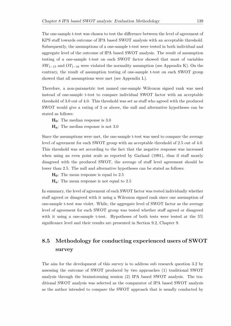
Chapter 8 IPA based SWOT analysis: Evaluation Methodology 139
The one-sample t-test was chosen to test the difference between the level of agreement ofKPS staff towards outcome of IPA based SWOT analysis with an acceptable threshold.Subsequently, the assumptions of a one-sample t-test were tested in both individual andaggregate level of the outcome of IPA based SWOT analysis. The result of assumptiontesting of a one-sample t-test on each SWOT factor showed that most of variablesSW1−15 and OT1−16 were violated the normality assumption (see Appendix K). On thecontrary, the result of assumption testing of one-sample t-test on each SWOT groupshowed that all assumptions were met (see Appendix L).
Therefore, a non-parametric test named one-sample Wilcoxon signed rank was usedinstead of one-sample t-test to compare individual SWOT factor with an acceptablethreshold of 3.0 out of 4.0. This threshold was set as staff who agreed with the producedSWOT would give a rating of 3 or above, the null and alternative hypotheses can bestated as follows:
H0: The median response is 3.0Ha: The median response is not 3.0
Since the assumptions were met, the one-sample t-test was used to compare the averagelevel of agreement for each SWOT group with an acceptable threshold of 2.5 out of 4.0.This threshold was set according to the fact that the negative response was increasedwhen using an even point scale as reported by Garland (1991), thus if staff mostlydisagreed with the produced SWOT, the average of staff level agreement should belower than 2.5. The null and alternative hypotheses can be stated as follows:
H0: The mean response is equal to 2.5Ha: The mean response is not equal to 2.5
In summary, the level of agreement of each SWOT factor was tested individually whetherstaff agreed or disagreed with it using a Wilcoxon signed rank since one assumption ofone-sample t-test was violet. While, the aggregate level of SWOT factor as the averagelevel of agreement for each SWOT group was tested whether staff agreed or disagreedwith it using a one-sample t-test. Hypotheses of both tests were tested at the 5%significance level and their results are presented in Section 9.2, Chapter 9.
8.5 Methodology for conducting experienced users of SWOTsurvey
The aim for the development of this survey is to address sub research question 3.2 byassessing the outcome of SWOT produced by two approaches (1) traditional SWOTanalysis through the brainstorming session (2) IPA based SWOT analysis. The tra-ditional SWOT analysis was selected as the comparator of IPA based SWOT analysisas the author intended to compare the SWOT approach that is usually conducted by

140 Chapter 8 IPA based SWOT analysis: Evaluation Methodology
the target organisation of the case study with the proposed SWOT approach. Addi-tionally, traditional SWOT analysis is practically in used SWOT approach as it is lesscomplicated among the SWOT approaches. It is expected that the comparison betweenthese two SWOT approaches will point out the differences between the currently usedapproach and the newly introduced approach of SWOT analysis.
8.5.1 Questionnaire design
The two questionnaires of experienced users of SWOT survey were divided into threesections. The first section provides information about the development of SWOT andconsists of steps for generating SWOT and the produced SWOT factors. The secondsection provides a list of questions asking participants to assess the quality and perceivedusefulness of SWOT presented in the first section of questionnaire. The last sectionof the questionnaire refers to the demographic data of MBA students such as gender,occupation and experience in using SWOT. The printed version of the two questionnairesare shown in Appendix M.1 (set A: IPA based SWOT analysis) and Appendix M.2 (setB: traditional SWOT analysis).
The differences between the two questionnaires are in the first and the second section ofthe questionnaire. In the first section, one describes information about the developmentof IPA based SWOT analysis (denoted as set A) whereas the other describes informationabout the development of traditional SWOT analysis. Specifically, the step for gener-ating SWOT shown in questionnaire set A is described following the IPA based SWOTframework (see Section 7.2, Chapter 7) and the produced SWOT factors presented inquestionnaire set A were obtained from the SWOT of KPS presented in Table 9.3. While,the step for generating SWOT shown in questionnaire set B is described following thetraditional approach for conducting SWOT analysis and the produced SWOT factorspresented in questionnaire set B were obtained from the brainstorming session of KPSstaff.
In the second section, questionnaire set A comprises of 12 questions whereas question-naire set B comprises of 10 questions. The first 10 questions are similar between ques-tionnaire set A and set B. Each question was rated on a five-point Likert scale and itsresponse was used to compare the difference of two SWOT approaches. The extra twoquestions of questionnaire set A were designed to ask participants about their opiniontoward the IPA based SWOT analysis.
Some of the 10 questions used in both questionnaires were adapted from a few researchstudies that were intended to examine the effectiveness of SWOT analysis (Hill andWestbrook, 1997; Coman and Ronen, 2009; Pai et al., 2013) and some were created by theauthor to fulfil the criteria for assessing SWOT. The 10 questions are shown in Table 8.7.Question number 1-4 were designed for checking common flaws of the SWOT analysis

Chapter 8 IPA based SWOT analysis: Evaluation Methodology 141
outcome. Question number 5 and questions number 6-7 were designed for checking thecomprehensibility and measurability of SWOT analysis outcome respectively. Questionnumber 8 was designed for checking that the SWOT factors were defined based on areasonable data source. And the last two questions were designed to check that theSWOT analysis outcome is actionable.
Table 8.7: List of questions in the experienced users of SWOT survey
Questions Source1. Strengths and weakness are explicit (clearly and unambigu-
ously formulated).Hill and Westbrook (1997)
2. The opportunities and the threats are explicit (clearly andunambiguously formulate).
Hill and Westbrook (1997)
3. All SWOT factors are not overgeneralisation. Hill and Westbrook (1997)
4. The strengths and weakness, and the opportunities andthreats are correctly classified as internal/external factors.
Hill and Westbrook (1997)
5. The SWOT factors comprehensively explain the depart-ment’s situation.
Pai et al. (2013)
6. All SWOT factors are measurable.
7. The order of SWOT factors makes decision-making easier.
8. The data source for this SWOT analysis is reliable. Pai et al. (2013)
9. The SWOT factors can be used as a starting point forstrategic planning.
Coman and Ronen (2009)
10. The SWOT factors provide useful information that sup-ports decision-making regarding strategic planning.
Pai et al. (2013)
8.5.2 Consistency of the translation between English and Thai versionof questionnaire
Since the participants are Thai, the questionnaire was translated from English intoThai. The consistency of the translation between the two languages was checked bythree Thai native-speakers who possess a good level of English in order to ensure thatthe Thai version of questionnaire could be understood by participants while preservingthe meaning of the original version.
In this step, three Thai native-speakers were asked individually to rate each statement orquestion on the degree of consistency between the two versions of languages by assigninga rating of +1 (consistency), 0 (undecided about whether Thai statement or question isconsistent with the English version) or −1 (no consistency). They were also requested
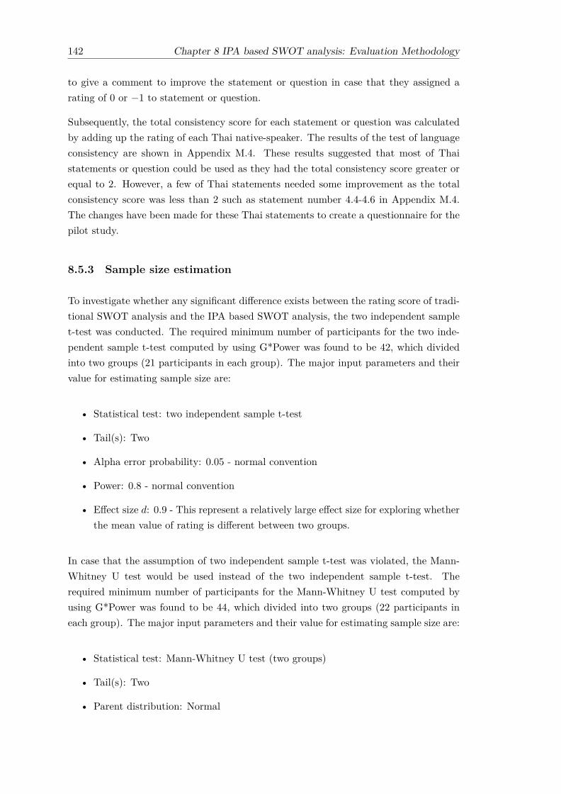
142 Chapter 8 IPA based SWOT analysis: Evaluation Methodology
to give a comment to improve the statement or question in case that they assigned arating of 0 or −1 to statement or question.
Subsequently, the total consistency score for each statement or question was calculatedby adding up the rating of each Thai native-speaker. The results of the test of languageconsistency are shown in Appendix M.4. These results suggested that most of Thaistatements or question could be used as they had the total consistency score greater orequal to 2. However, a few of Thai statements needed some improvement as the totalconsistency score was less than 2 such as statement number 4.4-4.6 in Appendix M.4.The changes have been made for these Thai statements to create a questionnaire for thepilot study.
8.5.3 Sample size estimation
To investigate whether any significant difference exists between the rating score of tradi-tional SWOT analysis and the IPA based SWOT analysis, the two independent samplet-test was conducted. The required minimum number of participants for the two inde-pendent sample t-test computed by using G*Power was found to be 42, which dividedinto two groups (21 participants in each group). The major input parameters and theirvalue for estimating sample size are:
• Statistical test: two independent sample t-test
• Tail(s): Two
• Alpha error probability: 0.05 - normal convention
• Power: 0.8 - normal convention
• Effect size d: 0.9 - This represent a relatively large effect size for exploring whetherthe mean value of rating is different between two groups.
In case that the assumption of two independent sample t-test was violated, the Mann-Whitney U test would be used instead of the two independent sample t-test. Therequired minimum number of participants for the Mann-Whitney U test computed byusing G*Power was found to be 44, which divided into two groups (22 participants ineach group). The major input parameters and their value for estimating sample size are:
• Statistical test: Mann-Whitney U test (two groups)
• Tail(s): Two
• Parent distribution: Normal

Chapter 8 IPA based SWOT analysis: Evaluation Methodology 143
• Alpha error probability: 0.05 - normal convention
• Power: 0.8 - normal convention
• Effect size d: 0.9 - This represent a relatively large effect size for exploring whetherthe mean value of rating is different between two groups.
8.5.4 Ethics
Experienced users of SWOT survey was conducted under ethics number ERGO/FPSE/18500 which received approval of the Ethics Committee of the University of Southamp-ton. This ethics number was presented in the participant information sheet (see detail inAppendix M.3) that was distributed to all MBA students who took part in the survey.
8.5.5 Pilot study
After improving the consistency of the translation, the questions for evaluating quality ofSWOT were examined for face validity by two experts who have experience in teachingand conducting SWOT analysis. It was found that the questions presented in thisquestionnaire appeared to be a valid measure for the SWOT quality. However, both ofthe experts raised their concern about the misclassification of SWOT factors in the casestudy.
Additional to the face validity, the questionnaire was piloted among four MBA studentsprior to the main study. They were asked to read the participant information sheet andthen responded to the pilot questionnaires. Specifically, participants of the pilot studywere divided into two groups of two participants to assess the two different SWOTapproaches: IPA based SWOT analysis and traditional SWOT analysis.
Two groups of participants were asked to complete the three main sections of the ques-tionnaire. Then, they were also asked to complete an additional section of the ques-tionnaire where they can give feedback about the questionnaire design and any othersuggestions they had for improving the questionnaire. The participants’ responses tothis additional section of the questionnaire are shown in Table 8.8.
Based on results of the pilot study shown in Table 8.8, the instruction of the introductionpart of survey was rewritten and five of the SWOT factors presented in questionnaireset B were cut-down by KPS staff to improve the questionnaire of the main study.
8.5.6 Data collection
MBA students were asked face to face to take part in the survey by the representative ofresearcher in their classroom during December 2015. They were divided into two equal

144 Chapter 8 IPA based SWOT analysis: Evaluation Methodology
Table 8.8: Opinion regarding to the design of questionnaire of experiencedSWOT user
Question Yes (%) No (%) Suggestions/Comments1. Are the instructions in the introduc-
tion part of survey clear?50.0 50.0
2. Is the case study described in Sec-tion 1 clear?
50.0 50.0
3. Are the case study, Figure and Ta-ble presented in Section 1 providinginformation for answering questionsin Section 2?
75.0 25.0
4. Is Figure 1 consistent with the casestudy and make it easier to under-stand the case study?
100.0 0.0
5. Are the questions in Section 2 clear? 100.0 0.0
6. Do you agree with the level of agree-ment used in the survey?
100.0 0.0
7. Are the questions in Section 3 clear? 100.0 0.0
8. Are there any comments that youwould like to make about the ques-tionnaire?
- It’s take long time to complete the questionnairedue to the difficulty of questionnaire. This could beaffect the accuracy of the questionnaire- There are too many SWOT factors in Table 1,suggested to reduce number of SWOT factors
independent groups of 22 participants. The first group of the participants were askedto evaluate IPA based SWOT analysis through the questionnaire set A (Appendix M.1). The second group of participants were asked to evaluate traditional SWOT analysisthrough the questionnaire set B (Appendix M.2).
Note that the sample size of 22 was equal to the minimum required sample size for dataanalysis using Mann-Whitney U test computed by G*Power (see sub-section 8.5.3). Datacharacteristics of the sample are shown in Table 8.9.
Table 8.9 lists general characteristics of MBA students who participated in the survey.For IPA based SWOT group, the sample of 22 MBA students comprise 3 (13.6%) malesand 19 (86.4%) females. Half of the sample are full-time students and the other halfare business owners (18.2%), others occupations included nurse, banker (13.6%) etc.95.5% of the overall sample possess experience in using SWOT analysis in academiawhile 18.2% of the overall sample possess 1-4 years practical experience in using SWOTanalysis. For the traditional SWOT group, the sample of 22 MBA students compriseof 6 (27.3%) males and 16 (72.7%) females. The majority are full-time students andbankers, and are about 36.4% and 31.8% of the overall sample respectively. All of the

Chapter 8 IPA based SWOT analysis: Evaluation Methodology 145
Table 8.9: General characteristics of two groups of MBA students (N=22)
Charaterisitic IPA based SWOT Traditional SWOTNumber Percentage Number Percentage
GenderMale 3 13.6 6 27.3Female 19 86.4 16 72.7
Age21 - 25 6 27.3 7 31.826 - 30 14 63.6 12 54.531 - 35 2 9.1 3 13.6> 35 0 0.0 0 0.0
OccupationPostgraduate student 11 50.0 8 36.4Business owner 4 18.2 3 13.6Government Officer 1 4.5 0 0.0Staff/ Sale Manager 1 4.5 0 0.0Staff/ Manager of Human Resources 1 4.5 1 4.5Staff/ Manager of Marketing 1 4.5 2 9.1Consultant 0 0.0 1 4.5Other. 3 13.6 7 31.8
Experience in using SWOT analysis in academiaNo 0 0.0 0 0.0Yes 21 95.5 22 100.0Missing value 1 4.5 0 0.0
Practical experience in using SWOT analysisNo 17 77.3 20 90.9Yes 4 18.2 2 9.1Missing value 1 4.5 0 0.0
sample possess experience in using SWOT analysis in academia while 9.1% of the overallsample possess 1-2 years practical experience in using SWOT analysis.
8.5.7 Data analysis method
To examine whether the IPA based SWOT analysis yielded a better quality of SWOTthan the traditional SWOT analysis, the response of the MBA students on those twoquestionnaires were analysed by using the two independent sample t-test to figure outwhether any significant difference exists between the mean ratings of two groups. Sub-sequently, the assumptions of the two independent sample t-test were tested and foundthat all variables represented the questions violated the normality assumption and somevariables violated the assumption of homogeneity of variance (see Appendix N).
Therefore, a non-parametric test named Mann-Whitney U test was used instead ofthe two independent sample t-test to determine if there were statistically significantdifferences in the mean ranks of the rating score in terms of the two groups. Although
146 Chapter 8 IPA based SWOT analysis: Evaluation Methodology
the Mann-Whitney U test does not require any assumptions related to the distribution,there are two important assumptions that should be checked (Pallant, 2005). First, thetwo sample groups drawn from the population are random and second, the two samplegroup are independent of each other.
These two assumptions can be observed regarding the survey design. The participantswere randomly selected from all MBA students at Faculty of Management Science, Sil-pakorn University, Thailand. They were also randomly assigned to each of the twogroups. Each participant can not appear in more than one group and the behaviourof one participant does not influence the behaviour of another. Thereby, ratings fromdifferent participants are independent. These assumptions therefore were met.
In order to run a Mann-Whitney U test, rating for each question was set as the depen-dent variable and type of SWOT approach which is split into two groups: IPA basedSWOT and Traditional SWOT was the independent variable. The null and alternativehypotheses of Mann-Whitney U test can be stated as follows:
H0: The distribution of ratings for the two groups are equalHa: The distribution of ratings for the two groups are not equal or the mean ranks
of the two groups are not equal.
Hypotheses of this test were tested at the 5% significance level and their results arepresented in Section 9.3, Chapter 9.
8.6 Summary
This chapter describes details of the methodologies related to the case study which wasconducted to demonstrate and evaluate the IPA based SWOT analysis. To demonstratehow the IPA based SWOT analysis can be used to generate SWOT, first the student sat-isfaction survey was undertaken at KPS and BKN following the survey research method.The data collected from the student satisfaction survey was then processed to generateSWOT of KPS regarding to the IPA based SWOT analysis framework. Through theframework, the student satisfaction survey data was analysed using multiple linear re-gression for calculating importance and computed the average as performance of eachSWOT factor which generated the IPA matrix of KPS and BKN. These IPA matriceswere then compared for classifying SWOT factors into four aspects of SWOT.
The SWOT of KPS was then evaluated by using the staff evaluation of SWOT surveyand the experienced users of SWOT survey to address the third research question. Since,there are no direct methods and tools for validating the effectiveness of SWOT analysis,the first survey aims to evaluate the SWOT from the viewpoint of the domain users ofSWOT in the case study which are the KPS staff. The participants of this survey wereasked to rate their level of agreement towards the SWOT of KPS. To test whether staff

Chapter 8 IPA based SWOT analysis: Evaluation Methodology 147
agreed or disagreed with the SWOT of KPS, the data collected through this survey wasanalysed at individual and aggregate level. For the individual level, level of agreementfor each SWOT factor of KPS was compared with an acceptable threshold using a one-sample Wilcoxon signed rank instead of one-sample t-test since the normality assumptionof t-test was not met. For the aggregate level, SWOT factors of KPS were grouped intofour aspects of SWOT and the average level of agreement for each group was computed.Subsequently, the one-sample t-test was used to compare the average level of agreementfor each SWOT group with an acceptable threshold.
The latter survey aims to evaluate the quality of SWOT from the viewpoint of experi-enced users of SWOT. The MBA students who possess related knowledge or real-worldexperiences in using SWOT analysis were invited to take part in this survey. To evaluatehow well the IPA based SWOT performs two versions of questionnaire were developedwhich are IPA based SWOT version and traditional SWOT version. The participantswere divided equally into two groups. Participants in each group were asked to examinethe SWOT presented in each version of the questionnaire and respond to the questionsrelated to the quality of SWOT. The Mann-Whitney U test was used instead of the twoindependent sample t-test to compare rating of individual questions between these twogroups since the normality assumption of t-test was not met.
The implementation of these methodologies produced SWOT of KPS, analytical resultsof the one-sample Wilcoxon signed rank test and the one-sample t-test, and analyti-cal results of the Mann-Whitney U test which are presented together with the resultsinterpretation in Chapter 9.


Chapter 9
IPA based SWOT analysis:Evaluation Results
By implementing the methodologies described in the previous chapter, SWOT of KPSand analytical results of SWOT evaluation were generated and are reported in thischapter. The aim of this chapter is to present SWOT of KPS which was generatedfollowing the IPA based SWOT analysis framework and describes the analytical resultsof the two surveys each of which is related to one of the sub research questions of thethird research question.
The chapter begins with an illustration of SWOT of KPS in Section 9.1 followed byanalytical results of staff evaluation on the SWOT of KPS presented in Section 9.2.Sections 9.3 reports analytical results of experienced users of SWOT analysis evaluationon the SWOT of KPS. The last section gives a summary of the chapter.
9.1 Results of IPA based SWOT analysis of the case study
The student satisfaction survey of KPS and BKN collected through the methodologydescribed in Section 8.2 was analysed through the methodology described in Section 8.3which produced the IPA matrix of the two departments and the SWOT of KPS. Thedetail of the two IPA matrices and SWOT of KPS is shown in the following sub-sections.
9.1.1 IPA matrix of the two departments
The IPA matrix of KPS and BKN was created individually by analysing data from thestudent satisfaction survey of the departments. Through the main tasks for constructingthe IPA matrix comprised calculation of importance and performance for individual
149
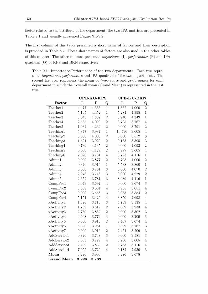
150 Chapter 9 IPA based SWOT analysis: Evaluation Results
factor related to the attribute of the department, the two IPA matrices are presented inTable 9.1 and visually presented Figure 9.1-9.2.
The first column of this table presented a short name of factors and their descriptionis provided in Table 8.2. These short names of factors are also used in the other tablesof this chapter. The other columns presented importance (I), performance (P) and IPAquadrant (Q) of KPS and BKN respectively.
Table 9.1: Importance-Performance of the two departments. Each row repre-sents importance, performance and IPA quadrant of the two departments. Thesecond last row represents the mean of importance and performance for eachdepartment in which their overall mean (Grand Mean) is represented in the lastrow.
CPE-KU-KPS CPE-KU-BKNFactor I P Q I P Q
Teacher1 4.477 4.335 1 1.362 4.000 2Teacher2 5.195 4.452 1 5.284 4.395 1Teacher3 3.043 4.387 2 3.940 4.349 1Teacher4 2.565 4.090 2 3.795 3.767 4Teacher5 1.934 4.232 2 0.000 3.791 2Teaching1 5.847 3.987 1 10.496 3.605 4Teaching2 3.086 4.006 2 0.000 3.512 3Teaching3 1.521 3.929 2 0.163 3.395 3Teaching4 0.739 4.135 2 0.000 4.093 2Teaching5 0.000 4.129 2 3.977 3.605 4Teaching6 7.020 3.761 4 3.723 4.116 1Admin1 0.000 3.877 2 0.708 4.000 2Admin2 9.346 3.916 1 5.538 3.860 1Admin3 0.000 3.761 3 0.000 4.070 2Admin4 2.978 3.748 3 0.000 4.279 2Admin5 2.652 3.781 3 8.989 4.116 1CompFac1 4.043 3.697 4 0.000 3.674 3CompFac2 5.868 3.684 4 6.955 3.651 4CompFac3 0.000 3.568 3 3.033 3.884 2CompFac4 5.151 3.426 4 3.850 2.698 4xActivity1 1.326 3.716 3 4.739 3.535 4xActivity2 1.739 3.819 2 7.009 3.233 4xActivity3 2.760 3.852 2 0.000 3.302 3xActivity4 4.608 3.774 4 0.000 3.209 3xActivity5 0.630 3.916 2 8.407 3.674 4xActivity6 6.390 3.961 1 0.399 3.767 3xActivity7 0.000 3.916 2 2.451 3.209 3AddService1 0.826 3.748 3 0.000 3.581 3AddService2 5.803 3.729 4 5.266 3.605 4AddService3 2.499 3.839 2 9.733 3.116 4AddService4 7.955 3.729 4 0.182 2.930 3Mean 3.226 3.900 3.226 3.678Grand Mean 3.226 3.789

Chapter 9 IPA based SWOT analysis: Evaluation Results 151
The red horizontal line and red vertical line in Figure 9.1-9.2 represent Grand Meanpresented in Table 9.1, which is computed as overall mean of importance and performanceof the two departments. The intersection of these lines created a four quadrants IPAmatrix labelled as “Q1 - Keep up the good work”, “Q2 - Possible overkill”, “Q3 - Lowpriority”and “Q4 - Concentrate here”.
Based on IPA matrix of KPS in Figure 9.1, the majority of factors are located in Quad-rant 2 and which are 13 out of 31 factors implying that resources committed to thesefactors would be better used in other quadrants in need of improved performance. Therewere seven factors located in Quadrant 4: Teaching6, ComFac1, ComFac2, ComFac4,xActivity4, AddService2, and AddService4 that require immediate attention for im-provement to meet student satisfaction. There were five factors located in Quadrant1: Teacher1, Teacher2, Teaching1, Admin2, and xActivity6 which are major factor forimproving student satisfaction.
Based on IPA matrix of BKN in Figure 9.2, the majority factors are located in Quadrant4 which are 10 out of 31 factors and they were competitive disadvantages for improvingstudent satisfaction of BKN. Quadrant 1 located the 5 factors for improving student sat-isfaction of this department which were: Teacher2, Teacher3, Teaching6, Admin2, andAdmin5. The two IPA matrices have a similar number of factors located in Quadrant 1which were competitive advantages for improving student satisfaction but different num-bers of factors located in Quadrant 4 which were competitive disadvantage for improvingstudent satisfaction. KPS has a fewer number of factors that need to be concentratedon for improving student satisfaction than BKN. This indicates a sign that KPS mayhave a competitive advantage over BKN.
9.1.2 SWOT matrix of CPE-KU-KPS
The results of IPA shown in Table 9.1 is then interpreted as strengths and weaknesses.Factors located in Quadrant 1 and Quadrant 2 were identified as strengths as theirperformance was higher than the grand mean of performance, whereas factors locatedin Quadrant 3 and Quadrant 4 were identified as weaknesses as their performance waslower than the grand mean of performance. The identification of strength and weaknessis shown in the second and third column of Table 9.2.
By comparing the factors of KPS and BKN that were previously labelled as strength(S) and weakness (W) in Table 9.2, opportunities (O) and threats (T) of KPS werethen identified regarding the SWOT identification table presented in Table 7.1. Finally,the SWOT of KPS with factor weight is presented in the fourth and fifth column ofTable 9.2.
Note that the factor weights were computed as the product of importance and perfor-mance of KPS shown in Table 9.1. Specifically, a positive value of performance was
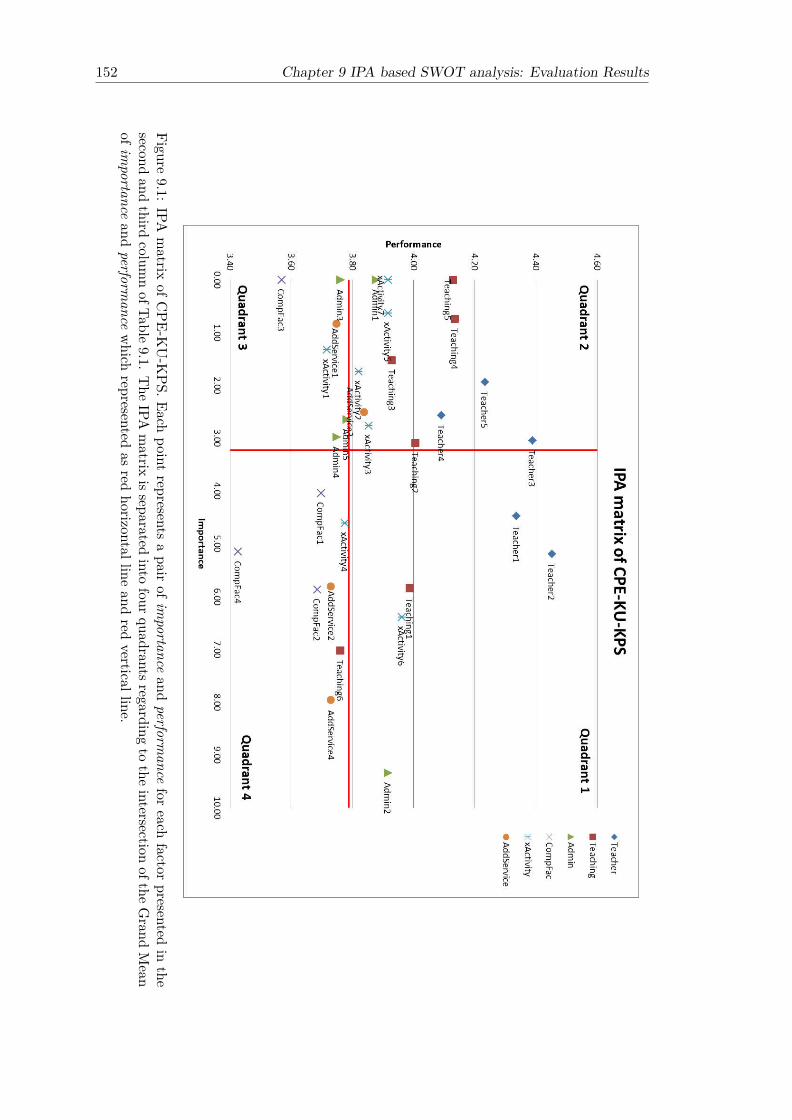
152 Chapter 9 IPA based SWOT analysis: Evaluation Results
Figure9.1:
IPAmatrix
ofCPE-K
U-K
PS.Eachpoint
representsapair
ofimportance
andperform
ancefor
eachfactor
presentedin
thesecond
andthird
columnofTable
9.1.The
IPAmatrix
isseparatedinto
fourquadrantsregardingto
theintersection
oftheGrand
Mean
ofimportance
andperform
ancewhich
representedas
redhorizontalline
andred
verticalline.
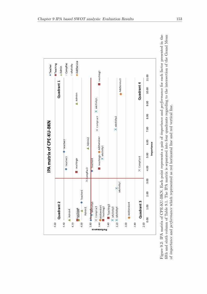
Chapter 9 IPA based SWOT analysis: Evaluation Results 153
Figu
re9.2:
IPA
matrix
ofCPE
-KU-B
KN.E
achpo
intrepresents
apa
irof
impo
rtan
cean
dpe
rfor
man
ceforeach
factor
presentedin
the
fifth
andsix
thcolumnof
Table9.1.
The
IPA
matrix
issepa
ratedinto
four
quad
rantsrega
rdingto
theintersectio
nof
theGrand
Mean
ofim
port
ance
and
perf
orm
ance
which
representedas
redho
rizon
tallinean
dredvertical
line.

154 Chapter 9 IPA based SWOT analysis: Evaluation Results
assigned to the strength and opportunity factors on the other hand a negative value ofperformance was assigned to the weakness and threat factors.
Table 9.2: Result of IPA based SWOT. Each row represents the factor whichlabelled as strength-weakness of the two departments, SWOT of CPE-KU-KPS,and its weight. For each factor, its weight is computed as the product of im-portance and performance of CPE-KU-KPS shown in Table 9.1
Strength - Weakness SWOT WeightFactor CPE-KU-KPS CPE-KU-BKN CPE-KU-KPS
Teacher1 S S S 19.411Teacher2 S S S 23.124Teacher3 S S S 13.349Teacher4 S W O 10.490Teacher5 S S S 8.187Teaching1 S W O 23.310Teaching2 S W O 12.364Teaching3 S W O 5.978Teaching4 S S S 3.056Teaching5 S W O 0.000Teaching6 W S T -26.403Admin1 S S S 0.000Admin2 S S S 36.598Admin3 W S T 0.000Admin4 W S T -11.160Admin5 W S T -10.026CompFac1 W W W -14.945CompFac2 W W W -21.619CompFac3 W S T 0.000CompFac4 W W W -17.648xActivity1 W W W -4.927xActivity2 S W O 6.640xActivity3 S W O 10.633xActivity4 W W W -17.389xActivity5 S W O 2.468xActivity6 S W O 25.310xActivity7 S W O 0.000AddService1 W W W -3.096AddService2 W W W -21.640AddService3 S W O 9.595AddService4 W W W -29.663
The SWOT of KPS in Table 9.2 was also represented as a SWOT matrix and shown inTable 9.3. Within a SWOT group, factors are prioritized by their weight. For strengthand opportunity, the factors with highest priority for maintaining or improving are “Ad-min2 - Knowledge of the information about courses, exams, activities of staff members”and “xActivity6 - Personal learning and thinking skills development activities” respec-tively. For weakness and threat, the factors with highest priority for improving are
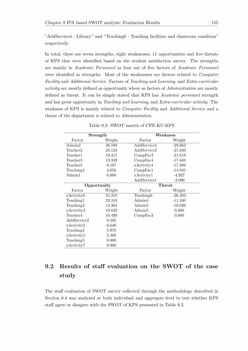
Chapter 9 IPA based SWOT analysis: Evaluation Results 155
“AddService4 - Library” and “Teaching6 - Teaching facilities and classroom condition”respectively.
In total, there are seven strengths, eight weaknesses, 11 opportunities and five threatsof KPS that were identified based on the student satisfaction survey. The strengthsare mainly in Academic Personnel as four out of five factors of Academic Personnelwere identified as strengths. Most of the weaknesses are factors related to ComputerFacility and Additional Service. Factors of Teaching and Learning, and Extra-curricularactivity are mostly defined as opportunity where as factors of Administration are mostlydefined as threat. It can be simply stated that KPS has Academic personnel strengthand has great opportunity in Teaching and Learning, and Extra-curricular activity. Theweakness of KPS is mainly related to Computer Facility and Additional Service and athreat of the department is related to Administration.
Table 9.3: SWOT matrix of CPE-KU-KPS
Strength WeaknessFactor Weight Factor Weight
Admin2 36.598 AddService4 -29.663Teacher2 23.124 AddService2 -21.640Teacher1 19.411 CompFac2 -21.619Teacher3 13.349 CompFac4 -17.648Teacher5 8.187 xActivity4 -17.389Teaching4 3.056 CompFac1 -14.945Admin1 0.000 xActivity1 -4.927
AddService1 -3.096Opportunity Threat
Factor Weight Factor WeightxActivity6 25.310 Teaching6 -26.403Teaching1 23.310 Admin4 -11.160Teaching2 12.364 Admin5 -10.026xActivity3 10.633 Admin3 0.000Teacher4 10.490 CompFac3 0.000AddService3 9.595xActivity2 6.640Teaching3 5.978xActivity5 2.468Teaching5 0.000xActivity7 0.000
9.2 Results of staff evaluation on the SWOT of the casestudy
The staff evaluation of SWOT survey collected through the methodology described inSection 8.4 was analysed at both individual and aggregate level to test whether KPSstaff agree or disagree with the SWOT of KPS presented in Table 9.3.

156 Chapter 9 IPA based SWOT analysis: Evaluation Results
For the individual level, the level of agreement of KPS staff towards each SWOT factorwas compared with a threshold of 3.0 using a one-sample Wilcoxon signed rank test.For the aggregate level, the average level of agreement of staff for each SWOT groupwas compared with a threshold of 2.5 using the one-sample t-test. Further details ofthe analytical method were provided in Sub-section 8.4.7 and the analytical results areshown in the following sub-sections.
9.2.1 Analytical results of staff evaluation on individual SWOT factor
Recall that there are 31 variables representing the level of agreement of KPS staff towardsindividual SWOT factor which were divided into 15 variables for strengths-weaknessesand 16 for opportunities-threats (denoted as variable named SW1−15, OT1−16). Thehypothesis using the one-sample Wilcoxon signed rank was tested at the 5% significancelevel. If the p-value is less than 0.05 then the median is significantly different from 3.0.The results are shown in Table 9.4 and 9.6 for strength-weakness and opportunity-threatfactors respectively.
Table 9.4: Result of one-sample Wilcoxon signed rank test for variable SW1−15
Null Hypothesis Median Sig. Decision regarding(2-tailed) the null hypothesis
The median of SW1 equals 3.0 3.00 1.000 RetainThe median of SW2 equals 3.0 3.00 0.180 RetainThe median of SW3 equals 3.0 3.00 0.102 RetainThe median of SW4 equals 3.0 3.00 0.083 RetainThe median of SW5 equals 3.0 3.00 0.107 RetainThe median of SW6 equals 3.0 2.00 0.003 RejectThe median of SW7 equals 3.0 3.00 0.480 RetainThe median of SW8 equals 3.0 2.50 0.096 RetainThe median of SW9 equals 3.0 2.50 0.034 RejectThe median of SW10 equals 3.0 2.00 0.004 RejectThe median of SW11 equals 3.0 3.00 0.058 RetainThe median of SW12 equals 3.0 2.00 0.002 RejectThe median of SW13 equals 3.0 2.00 0.001 RejectThe median of SW14 equals 3.0 2.00 0.002 RejectThe median of SW15 equals 3.0 2.00 0.004 Reject
According to Table 9.4, there were 7 out of 15 variables represented strengths-weaknessesthat have the median of staff agreement level statistically significantly different from 3.0.Among seven variables with their level of agreement of KPS staff lower than 3.0, six ofthem are weaknesses. Detail of these variables is shown in Table 9.5.
With regard to Table 9.4 and Table 9.5, it is clearly shown that staff agreed with morestrength factors than weakness factors. As 6 out of 8 of weakness factors were not agreedby KPS staff whereas 1 out of 7 of strength factors were not agreed by KPS staff.
According to Table 9.6, 3 out of 16 variables represented opportunity factors that havethe median of staff agreement level statistically significantly different from 3.0 namely

Chapter 9 IPA based SWOT analysis: Evaluation Results 157
Table 9.5: List of strength-weakness variables that their level of staff agreementis lower than 3.0
Variable Factor DetailSW6 Admin1 Knowledge of rules and procedures of non-academic staff
membersSW9 CompFac2 Lack of availability of computer facilities for studentsSW10 CompFac4 Lack of availability of printing and photocopying facilitiesSW12 xActivity4 Poor arrangement of health development activitiesSW13 AddService1 Lack of financial aid provided for studentsSW14 AddService2 Lack of medical support provided for studentsSW15 AddService4 Lack of availability of library facilities
Table 9.6: Result of one-sample Wilcoxon signed rank test for variable OT1−16
Null Hypothesis Median Sig. Decision regarding(2-tailed) the null hypothesis
The median of OT1 equals 3.0 3.00 0.655 RetainThe median of OT2 equals 3.0 3.00 1.000 RetainThe median of OT3 equals 3.0 3.00 0.014 RejectThe median of OT4 equals 3.0 3.00 0.414 RetainThe median of OT5 equals 3.0 3.50 0.008 RejectThe median of OT6 equals 3.0 3.00 1.000 RetainThe median of OT7 equals 3.0 3.00 0.317 RetainThe median of OT8 equals 3.0 3.00 0.257 RetainThe median of OT9 equals 3.0 3.00 0.102 RetainThe median of OT10 equals 3.0 3.00 0.414 RetainThe median of OT11 equals 3.0 3.00 0.180 RetainThe median of OT12 equals 3.0 3.00 0.025 RejectThe median of OT13 equals 3.0 3.00 0.564 RetainThe median of OT14 equals 3.0 3.00 0.083 RetainThe median of OT15 equals 3.0 3.00 0.083 RetainThe median of OT16 equals 3.0 3.00 1.000 Retain
OT3, OT5 and OT12. For OT3 and OT12, the median of staff agreement level were lowerthan 3.0 whereas, for OT5 the opposite was true: the median of staff agreement levelwere higher than 3.0. Detail of these variables is shown Table 9.7.
Table 9.7: List of opportunity variables that their level of staff agreement isdifferent from 3.0
Variable Factor DetailOT3 Teaching2 Increasing E-learning resources to support student learningOT5 Teaching5 Increasing accurate and up-to-date course unit contentOT12 xActivity3 Improving the arrangement of moral development activities
With regard to Table 9.6 and Table 9.7, KPS staff positively agreed with OT5 and staffagreed with other variables except OT3 and OT12. KPS staff also agreed with all fivevariables of threat factors namely OT6 - OT10.
In summary, for each SWOT group only weakness factors have a percentage of agreementby KPS staff less than 50% while the other three groups have percentage of agreement

158 Chapter 9 IPA based SWOT analysis: Evaluation Results
by KPS staff up to 80% as shown in Table 9.8. It can be reasonably concluded that 3out of 4 aspects of KPS SWOT have a high face validity.
Table 9.8: Summary of agreed SWOT factors
Group of SWOT Variable Number Number of Percentage ofof factors agreed factors agreed factors
Strength SW1 - SW7 7 6 85.71%Weakness SW8 - SW15 8 2 25.00%
Opportunity OT1 - OT5, 11 9 81.82%OT11 - OT16
Threat OT6 - OT10 5 5 100.00%
9.2.2 Analytical results of staff evaluation on the group of SWOT fac-tor
Recall that there are four variables named Savg, Wavg, Oavg, Tavg representing theaverage level of agreement of staff for each SWOT group. The hypothesis using theone-sample t-test was tested at the 5% significance level. If the p-value is less than 0.05then the mean response is significantly different from 2.5. The descriptive statistic ofvariables and the result of the one-sample t-test is shown in Table 9.9. Additionally, themeans of response across the four variables is visually presented as simple error bars inFigure 9.3.
Figure 9.3: Simple error bar of the four variables of each SWOT group. Themean is represented by a dot, a line represents standard error of the mean, ared horizontal line is represented the threshold score of 2.5.
With regards to Table 9.9, average score of strength factors (M = 2.93, SD = 0.36) ishigher than the threshold score of 2.5, a statistically significant mean difference of 0.43,

Chapter 9 IPA based SWOT analysis: Evaluation Results 159
Table 9.9: Result of the One-sample t-test for each SWOT group (Test value is2.5)
Variable Mean SD Mean Difference t df p (2-tailed)Savg 2.93 0.355 0.43 3.196 6 0.019Wavg 2.35 0.224 -0.15 -1.916 7 0.097Oavg 3.19 0.184 0.69 12.389 10 <0.001Tavg 2.89 0.179 0.39 4.811 4 0.009
t(6) = 3.196, p = 0.019. Since p < 0.05, the null hypothesis is rejected and it can beconcluded that the mean of average strength factors is statistically significantly differentfrom the threshold score of 2.5.
Average score of weakness factors (M = 2.35, SD = 0.22) is lower than the thresholdscore of 2.5, a statistically significant mean difference of -0.15, t(7) = -1.916, p = 0.097.Since the p-value is greater than 0.05 therefore the null hypothesis is retained and it canbe concluded that the mean of average weakness factors is not statistically significantlydifferent from 2.5.
Average score of opportunity factors (M = 3.19, SD = 0.18) is higher than the thresholdscore of 2.5, a statistically significant mean difference of 0.69, t(10) = 12.389, p = 0.000.Since p < 0.001, the null hypothesis is rejected and it can be concluded that the meanof average opportunity factors is statistically significantly different from the thresholdscore of 2.5.
Average score of threat factors (M = 2.89, SD = 0.18) is higher than the thresholdscore of 2.5, a statistically significant mean difference of 0.39, t(4) = 4.811, p = 0.009.Since p < 0.05, the null hypothesis is rejected and it can be concluded that the mean ofaverage threat factors is statistically significantly different from the threshold score of2.5.
In summary, the average of agreement level toward weakness is slightly lower than, butnot significantly different to the threshold score of 2.5 (p-value > 0.05). Thus it canbe concluded that the mean of average weakness items is equal to 2.5 indicating thatKPS staff seemed to agree with the weakness of KPS produced from IPA based SWOTanalysis. The average of agreement level toward strength, opportunity and threat arestatistically significantly different from the threshold score of 2.5 and their means arehigher than 2.5 which also indicated that KPS staff seemed to agree with the strength,opportunity and threat of KPS produced from IPA based SWOT analysis.
Specifically, the average of agreement level towards strength and threat is close to 3.0and the average of agreement level toward opportunity is higher than 3.0. To confirmthat staff were mostly agreed with these three aspects of KPS SWOT, the one-samplet-test was further conducted with the threshold of 3.0 which means agree. The result

160 Chapter 9 IPA based SWOT analysis: Evaluation Results
is shown in Table 9.10 and the means of response across the three variables is visuallypresented as simple error bars in Figure 9.4.
Figure 9.4: Simple error bar of the three variables of SWOT group. The meanis represented by a dot, a line represents standard error of the mean, a redhorizontal line is represented the threshold score of 3.0
Table 9.10: Result of the One-sample t-test for three SWOT group (Test valueis 3.0)
Variable Mean SD Mean Difference t df p (2-tailed)Savg 2.93 0.355 -0.07 -0.533 6 0.613Oavg 3.19 0.184 0.19 3.390 10 0.007Tavg 2.89 0.179 -0.11 -1.425 4 0.227
With regards to Table 9.10, the average of agreement level toward opportunity is statis-tically significantly different from 3.0 and its value is higher than 3.0, and the averageof agreement level toward strength and threat is lower than, but not statistically sig-nificantly different to 3.0. It can be confirmed that KPS staff were mostly agreed withstrength, opportunity and threat of KPS produced from IPA based SWOT analysis.Taken together, results from Table 9.9 and Table 9.10 suggest that KPS staff agreedwith factors within each SWOT aspect.
The analytical results at both individual and aggregate level of SWOT factors providesanswer to the sub research question 3.1. As they consistently indicated that KPS staffmostly agreed with strengths, opportunities and threats of their department and theanalytical result of weaknesses in aggregate level showed that KPS staff were agreed onweaknesses. The analytical result of weaknesses in individual level showed that only25.00% of weakness factors were agreed by staff. These results will be discussed inChapter 10.

Chapter 9 IPA based SWOT analysis: Evaluation Results 161
9.3 Results of SWOT experienced users evaluation on theSWOT of the case study
The experienced users of SWOT survey collected through the methodology describedin Section 8.5 was analysed to determine whether there is a difference in rating scoreregarding the quality of SWOT of KPS produced through the two SWOT approaches:IPA based SWOT analysis and Traditional SWOT analysis.
Specifically, 44 participants of this survey were divided equally into two groups. Thefirst group rated the 10 questions for IPA based SWOT analysis while the second grouprated the 10 questions for traditional SWOT analysis. The mean and standard deviationof rating score of the two SWOT approaches are presented in Table 9.11.
Table 9.11: The mean and standard deviation of rating score on 10 questionsregarding the two SWOT approaches
Question IPA based SWOT Traditional SWOTMean Std. Deviation Mean Std. Deviation
1 3.364 0.790 3.227 0.7522 3.318 0.568 3.500 0.6733 3.364 0.790 3.227 0.7524 3.000 0.926 3.136 0.8345 3.364 0.902 3.909 0.4266 3.864 0.560 3.409 0.7347 4.045 0.576 3.273 0.8278 3.409 1.008 4.182 0.5019 3.500 0.740 4.091 0.52610 3.409 0.854 4.091 0.294
The hypothesis was tested using Mann-Whitney U at the 5% significance level. If theasymptotic p-value is less than 0.05 then, there are statistically significant differencesin the mean ranks of the rating score between the two groups. The results of Mann-Whitney U test are shown in Table 9.12.
The column Mean Rank in Table 9.12 indicates which group can be considered as havingthe higher rating score. For each question, the group with the higher mean rank has thehigher rating score than another. The column U statistic and Asymp. Sig in Table 9.12provides the test value and the asymptotic significance value of the test respectively.The following observations can be drawn from the interpretation of this table.
(1) The mean rank of rating score for the question numbers 1-4 between the two groupsof SWOT approaches was not statistically significantly different. These questions arerelated to common flaws of the SWOT analysis outcome. Therefore, it can be concludedthat the two SWOT approaches have about the same quality measured on the commonflaws of the SWOT analysis.

162 Chapter 9 IPA based SWOT analysis: Evaluation Results
Table9.12:
Results
oftheMann-W
hitneyU
test(N
=22)
Questionnaire
itemMean
Rank
Ustatistic
Asym
p.IPA
basedSW
OT
TraditionalSWOT
Sig.(2-tailed)
1.Strengthsandweaknessareexplicit(clearly
andunam
biguouslyform
ulated).23.50
21.50220.00
0.572
2.Opportunities
andthreats
areexplicit
(clearlyand
unambigu-
ouslyform
ulated).20.89
24.11206.50
0.348
3.SW
OT
factorsare
notovergeneralised
23.4121.59
222.000.613
4.SW
OT
factorsare
notcorrectly
classifiedas
internal/externalfactors
21.4823.52
219.500.577
5.SW
OT
factorsare
comprehensively
explainthe
department’s
situation18.48
26.52153.50
0.015
6.AllSW
OT
factorsshow
nare
measurable
25.8919.11
167.500.043
7.The
orderofSW
OT
itemsmakes
decision-making
easier.27.84
17.16124.50
0.002
8.The
datasource
forthis
SWOT
analysisis
reliable17.57
27.43133.50
0.005
9.The
SWOT
itemscan
beused
asastarting
pointfor
strategicplanning
18.0926.91
145.000.006
10.The
SWOT
itemsprovide
usefulinformation
thatsupports
decision-making
regardingstrategic
planning17.05
27.95122.00
0.001

Chapter 9 IPA based SWOT analysis: Evaluation Results 163
(2) The mean rank of rating score for the question numbers 5 and 8-10 in the TraditionalSWOT analysis group was higher than and statistically significantly different from thatof the IPA based SWOT analysis group. Question number 5 and number 8 are re-lated to the comprehensibility of SWOT analysis outcome and reliability of data sourceof SWOT analysis respectively. Question number 9-10 are related to action-ability ofSWOT analysis outcome. Hence, it can be concluded that Traditional SWOT analysisis better than IPA based SWOT analysis in terms of comprehensibility, reliability ofdata source, and action-ability.
(3) The rating score of the question numbers 6-7 in the IPA based SWOT analysisgroup was higher than and statistically significantly different from that of the TraditionalSWOT analysis group. These questions are related to measurability of SWOT analysisoutcome. Therefore, it can be concluded that IPA based SWOT analysis is better thanTraditional SWOT analysis in terms of measurability.
Taken together, results from Table 9.11 and Table 9.12 suggest that quality for all eval-uation aspects of the two SWOT approaches are considered acceptable as the averagescores are centred around 3.00 to 4.00 and no SWOT approach is superior to another inall evaluation aspects. Hence, the answer to the sub research question 3.2. is that thequality of the outcome of IPA based SWOT analysis is considered acceptable. Discus-sions of these results will be presented in Chapter 10.
9.4 Summary
This chapter reports the results of the three surveys - student satisfaction survey, staffevaluation of SWOT survey and experienced users of SWOT survey which were con-ducted to demonstrate and evaluate the IPA based SWOT analysis so as to help answerthe third research question. To demonstrate how the IPA based SWOT analysis canbe used to generate SWOT, the student satisfaction surveys of KPS and BKN wereanalysed through the IPA based SWOT analysis framework which generated SWOT ofKPS. The SWOT of KPS consists of factors classified as 7 strengths, 8 weaknesses, 11opportunities and 5 threats. All SWOT factors are prioritized by their weight computedon the basis of importance-performance analysis. The factor with the larger magnitudeof the weight has higher priority for maintenance or improvement than the factor withthe smaller one.
For the purpose of evaluation, first the SWOT of KPS was assessed to determine whetherKPS staff agreed or disagreed with it through the staff evaluation of SWOT survey. Alldata collected from the staff evaluation of SWOT survey was analysed at individualand aggregate level of SWOT factors using a one-sample Wilcoxon signed rank and theone-sample t-test respectively. The analytical results of these statistical tests showed

164 Chapter 9 IPA based SWOT analysis: Evaluation Results
that the staff of KPS agreed with SWOT of KPS. This suggested that the outcome ofIPA based SWOT analysis accurately reflected the KPS’s situation.
Second, the SWOT of KPS produced from IPA based SWOT analysis was comparedwith another version of SWOT of KPS produced from traditional SWOT approach, byexperienced users of SWOT to determine whether there is a difference in rating scoreregarding the quality of SWOT of KPS produced through the two different SWOTapproaches. All data collected from experienced users of SWOT survey was analysedusing Mann-Whitney U test. The analytical results of Mann-Whitney U test suggestthat no SWOT approach was superior to another in all evaluation aspects.
These results demonstrated that the IPA based SWOT analysis can be used to processand analyse customer satisfaction survey to generate SWOT that accurately reflects theorganisation’s situation. In addition, the quality of the outcome of IPA based SWOTanalysis was considered acceptable compared with the outcome of traditional SWOTanalysis. These results will be further discussed in Chapter 10.

Chapter 10
Discussion
Having conducted the empirical comparison of importance measure techniques and thecase study in the previous chapters, this chapter reflects upon and discusses their resultsthat help to answer the research questions of this study. Section 10.1 discusses resultsand methodology related to the empirical comparison of importance measure techniques.Section 10.2 discusses about pros and cons of IPA based SWOT analysis. Section 10.3discusses evaluation results of IPA based SWOT analysis and finally Section 10.4 dis-cusses the limitations of the research.
10.1 Discussion of Empirical comparison
There has been an ongoing argument over whether self-stated or implicitly derived meth-ods should be used in measuring importance (Gustafsson and Johnson, 2004; Fontenotet al., 2007) or even a debate on the most appropriate method to obtain implicit impor-tance (Feng et al., 2014; Lai and Hitchcock, 2015).
Particularly, over the years many different IPA variations have emerged with the mainfocus on a method to indirectly measure importance. Many researchers have claimed thattheir complicated mechanism works best without conducting an empirical comparisonof evaluation metrics (Deng et al., 2008a; Hu et al., 2009; Krešić et al., 2013).
To date, there have been a few empirical studies that compared the different methods formeasuring importance against a set of evaluation criteria (Azzopardi and Nash, 2013).Hence, the empirical comparison was set out with the aim of identifying a suitabletechnique for measuring importance in this thesis.
The results of the empirical comparison indicated MLR is the best importance measuretechnique whereas self-stated importance measure using direct-rating scales is the worstimportance measure technique in terms of the three evaluation metrics. This finding
165

166 Chapter 10 Discussion
supports the claim that implicitly derived importance measures should be used in mea-suring importance rather than the self-stated importance measure, and MLR is the mostfavourable technique for implicitly derived importance.
The finding in favour of MLR raises the case that a simple technique works best. How-ever, the importance obtained from MLR needs to be used with caution, as this techniqueis likely to produce negative coefficients. A full discussion of the empirical results canbe found in Section 6.4 while discussions related to the methodology of empirical com-parison are provided in the following paragraphs.
• Evaluation metricsEvaluation metrics play a critical role in determining the best importance mea-surement techniques. Idealistically, the best comparison of alternative importancemeasurement techniques would be to develop different action plans according toimportance measurement technique and observe business performance measuressuch as Return on Investment (ROI). However, considering time and cost to carryout such an experiment, it is practically hard or even impossible to carry out(Hauser, 1991).
As a matter of fact, researchers of previous comparative studies specified a setof evaluation metrics based on their judgement on what is a good importancemeasure. Three evaluation metrics namely predictive validity, diagnosticity, anddiscriminating power which were most used in the previous comparative studieswere selected to use in the present empirical comparison. The use of the multiplemetrics not only allows the author to investigate different aspects of the importancemeasures but also maximizes the accuracy of the evaluation.
Among the three selected evaluation metrics, predictive validity (ability to pre-dict actual overall customer satisfaction) is the most used evaluation metrics inthe previous comparative studies (Hauser, 1991; Gustafsson and Johnson, 2004;Chrzan and Golovashkina, 2006; Taplin, 2012b). However, it is considered to beproblematic for a comparison as it allows MLR and OLR to gain an advantageover other techniques, because their importance was calculated on the same datawhich was used for measuring predictive validity as correlation coefficients (Neslin,1981) therefore maximizing predictive validity.
Concerning this issue, the relative predictive validity (ability to predict customer-reported priority) is a good alternative choice of the predictive validity since aprediction of customer preference rank-order provides a fair comparison amongtechniques. However, to measure this metric cause survey respondent to do anadditional task which might affect survey response rate. Additionally, this presentstudy used the two surveys from other research studies that did not provide thecustomer preference rank-order. Therefore, the relative predictive validity was notfit to use in the context of this empirical study.
Chapter 10 Discussion 167
Turning now to the weight of evaluation metrics, this is another key element thatshould be considered when the multiple metrics are used. Currently, either aset of metrics or the most critical criteria for identifying the importance measuretechnique has not been yet established. This study weighted all three evaluationmetrics equally. This weighting scheme is similar to the weighting scheme used inthe previous studies by Gustafsson and Johnson (2004); Chrzan and Golovashkina(2006).
On the other hand, this weighting scheme differs from the one used in the study byPokryshevskaya and Antipov (2014). Their study used a more complicate weighingscheme in which the weights of evaluation metrics were varied using an iterativeMonte-Carlo technique. This is because Pokryshevskaya and Antipov (2014) couldnot identify a clear winning technique if the two evaluation metrics were equallyweighted, as there was not much difference between the ranked mean of the topsix techniques. In contrast, there was a clear difference between the ranked meanof the top three techniques compared in this study (see Table 6.7). Hence, it isnot necessary to conduct such a complicate weighting scheme in this study.
• Use of the baseline evaluation metricIt is good practice to establish a baseline measurement for each metric. In thisempirical study, the baseline measurements were computed under the criterionthat all attributes are equally important in another word all have importancevalue equal to one.
The baseline measurements then served as a point of reference to assess the effect ofimportance measures by different techniques. By comparing the value of evaluationmetrics namely predictive validity and discrimination power of each techniquewith that of the baseline measurements, it shows that importance measures ofall techniques do improve both predictive validity and discrimination power (seeTable 6.4 and Table 6.6), thereby, demonstrating the merit of importance measure.
The use of baseline measurements shows that the present empirical study was care-fully conducted which reveals such an interesting finding as previously stated. Inspite of its benefit, the majority of the previous studies did not set any baselinemeasurement except the work by Hauser (1991). Hence, this study recommendsresearchers in IPA field to establish baseline measurements when comparing im-portance measuring techniques.
• Number of datasets usedWith regard to number of datasets, this empirical study used three datasets indifferent business areas while the majority of the previous studies conducted thecomparison on one or two dataset(s). The fact that the three datasets were usedin this study allows the author to infer generality of the findings reported in Sec-tion 6.2.4 with confidence.

168 Chapter 10 Discussion
However, the size of the datasets used in this study is considered small (hundredrecords) and moderate (thousand records) when compared with the other contextof a data mining application (Azzalini et al., 2012, p. 193). Further comparison ofimportance measuring techniques on a bigger scale of dataset would be beneficialfor the IPA studies.
10.2 Discussion of IPA based SWOT analysis and its ap-plication
According to a demonstration of IPA based SWOT analysis application through a casestudy of HEIs, it shows that IPA based SWOT analysis can be used in supportingstrategic planning in a real-world situation. Although the application of IPA basedSWOT analysis in this study was illustrated in the specific field, the IPA based SWOTanalysis can be used widely in the other business areas where SWOT analysis has beenseen applicable and the customer satisfaction surveys are generally conducted.
As its name conveys, a distinctive characteristic of the IPA based SWOT analysis is thatit utilizes IPA to systematically generate SWOT factors based on a customer satisfactionsurvey. To the best of the author’s knowledge, this is the first study that applies IPA ingenerating SWOT factors.
The combined use of the IPA and SWOT analysis yields quantitative SWOT factorsregarding the importance and performance obtained from customer satisfaction surveys.In addition, it yields customer-oriented SWOT factors which guarantee that the capa-bilities perceived by an organisation are recognized and valued by the customers anddiminish bias of an organisation’s staff. This facilitates an organisation to efficiently for-mulate strategic planning for maintaining or enhancing customer satisfaction, therebygaining a competitive advantage.
It can be stated that IPA based SWOT analysis diminishes two major drawbacks oftraditional SWOT analysis as well as bridges the gap of the current two main streamsof SWOT approaches: quantitative SWOT analysis (Kurttila et al., 2000; Kangas et al.,2001; Lee and Lin, 2008) and customer-oriented SWOT analysis (Dai et al., 2011; Paiet al., 2013). The quantitative approach can make SWOT factors commensurable butthey are identified solely on an organisation’s perspective without considering the cus-tomer’s perspective. On the other hand, the customer-oriented approach generatesSWOT factors from a customer’s perspective but it has no means to prioritize SWOTfactors as they are extracted from unstructured data sources such as e-mail, online blog,and social media content.
Considering data sources for the different SWOT analysis approaches and their associ-ated analytical techniques (Table 10.1), IPA based SWOT analysis is the only approach

Chapter 10 Discussion 169
that uses structured data as an input data source while the others use unstructureddata. The IPA based SWOT analysis performs a deeper analysis of data from customersatisfaction surveys that the organisation generally collects. Hence, it provides morecredible SWOT factors than traditional and quantitative SWOT analysis that identifySWOT based on staff opinion usually with no supporting evidence.
The IPA based SWOT analysis also gains an advantage over the customer-orientedSWOT analysis in terms of simplicity since it requires less complicated analytical tech-niques for processing data than the customer-oriented SWOT analysis that requirescomputational linguistics to process customer opinion in the form of text, both at syn-tax and semantic level.
Table 10.1: Summary of data sources for the different SWOT analysis ap-proaches and their associated analytical techniques
SWOT Data source Data type Analyticalapproaches technique
Traditional SWOTanalysis
Individual opinion of organ-isation’s staff who attend abrain storming session
Unstructured dataas personal opinion
n/a
QuantitativeSWOT analysis
Same as above Same as above AHP, ANP
Customer-orientedSWOT analysis
e-mail, online blog, and socialmedia content
Unstructured data,text
NLP, Text mining,Sentimental analy-sis
IPA based SWOTanalysis
Customer satisfaction surveymeasured in Likert scales
Structured data,numeric
IPA
To take full advantages of IPA based SWOT analysis, all four steps for developing IPAbased SWOT analysis (see Section 7.2) need to be carefully conducted. Among thefour steps, the most critical one is the first step which involves the undertaking of acustomer satisfaction survey. This is because a list of SWOT factors is dependent onthe questionnaire items/questions that represent attributes of the organisation beingsurveyed. Therefore, the attributes need to be carefully selected to ensure that theevaluative attributes that are important to the customer are not overlooked as discussedby Martilla and James (1977) who suggested that attributes should be listed based ona thorough literature review in each application area or by interviews. The attributesassociated with the student satisfaction survey conducted in this thesis were selectedbased on a list of attributes defined in previous studies of student satisfaction (Siskosand Grigoroudis, 2002; Silva and Fernandes, 2011; Grebennikov and Shah, 2013).
Another criteria in undertaking a customer satisfaction survey is that two identicalquestionnaires are required by IPA based SWOT analysis so that each factor of targetorganisation and its competitor can be compared and categorised into four aspects ofSWOT. As the two organisations are willing to corporate in the case study, it is not

170 Chapter 10 Discussion
difficult to fulfil this requirement in conducting the case study of this thesis. However,this requirement of the two identical questionnaires may not be practical which raisesthe issue of how can the organisation collect the satisfaction survey from its competi-tor’s customers. One possible way to resolve this issue is to use customer satisfactionmeasurements on a national scale such as ACSI, UKCSI, and so forth, as a data sourceof IPA based SWOT analysis since, these measurements of customer satisfaction at anational level provide uniform and comparable information that allows for systematicbenchmarking across firms.
10.3 Discussion of evaluation result of IPA based SWOTanalysis
The two surveys described in Chapter 8 for the purpose of evaluating IPA based SWOTanalysis. This section provides discussions of the results of these two surveys which werereported in Chapter 9.
10.3.1 Discussion of staff evaluation on the SWOT of the case study
A survey of KPS staff evaluation on SWOT of KPS, the results of IPA based SWOTanalysis, set out to assess whether KPS staff agree or disagree with the SWOT of KPS.Data analysis was carried out at individual (each SWOT factor) and aggregate level (agroup of SWOT factors).
The analytical results at both individual and aggregate level of SWOT factors consis-tently indicated that KPS staff mostly agreed with strengths, opportunities and threatsof their department. However, analytical results toward the weaknesses are slightly dif-ferent at the two analysis levels. The analytical result of weaknesses at aggregate levelshowed that KPS staff seem to agree on weaknesses whereas the opposite was true forthe analytical result of weaknesses at the individual factor level.
The aggregate results suggest that KPS staff agreed with all aspects of the IPA basedSWOT analysis for KPS. This demonstrates a validity of the IPA based SWOT methodin a real-world case and confirms that it can thus be used in providing useful informationfor strategic planning. With regard to the results at the individual factor level, there isa low face validity on Weaknesses (W), as only 25.00% of weakness factors were agreedby staff. While other aspects of SWOT have high face validity, for example up to 80%of Strength (S), Opportunity (O) and Threat (T) factors were agreed by staff.
Although the result of the Weaknesses (W) factor at the individual factor level shows apresence of low face validity of IPA based SWOT analysis, it reveals another interest-ing finding that staff seem to blind on their organisation’s weaknesses. The most likely
Chapter 10 Discussion 171
explanation for the small percentage of staff agreement toward weaknesses is an unwill-ingness to admit individual weaknesses as highlighting weaknesses can draw attentionto areas of the organisation that one has badly operated. Thus, one reacts in a stateof denial1 about them. According to Humphreys (2007), many senior managers denyto talk about weaknesses objectively as doing so imply criticism of the way that theorganisation has been managed.
10.3.2 Discussion of SWOT experienced users evaluation on the SWOTof the case study
Experienced users of SWOT evaluation set out to assess whether there is a differentin rating the quality of SWOT of KPS produced through the two SWOT approaches:IPA based SWOT analysis and traditional SWOT analysis. The descriptive statisticssuggested that quality for all evaluation aspects of the two SWOT approaches was con-sidered acceptable as the average scores ranged from moderate to good and the analyt-ical results indicated that no SWOT approach was superior to another in all evaluationaspects.
Specifically, three findings can be drawn from the analytical results. The first findingsuggests that common flaws of SWOT analysis were similar in both SWOT approaches.However, their rating scores regarding common flaws were considered acceptable.
Regarding the second finding, traditional SWOT analysis is better than IPA basedSWOT analysis in term of comprehensibility, reliability of data source, and action-ability. This finding was unanticipated and suggests that comprehensibility, reliabilityof data source and action-ability of IPA based SWOT analysis are not clearly perceivedby experienced SWOT users.
This result may be explained by the fact that information provided in the survey maynot be enough for them to perceive these characteristics of IPA based SWOT analysis.Additionally, experienced SWOT users may be influenced by a primacy effect2 as tradi-tional SWOT analysis has been used for decades and experienced SWOT users are morefamiliar with it than IPA based SWOT analysis. In this circumstance, the experiencedSWOT users might rate a higher score for the outcome of traditional SWOT relativeto IPA based SWOT analysis. A recent study by Bansback et al. (2014), showed thatprimacy effect is also prominent in making decisions regarding the treatment options forpatients.
1Denial is an ego-defence mechanism that unconsciously operates to reduce anxiety by refusing toperceive the unpleasant aspects of external reality (New World Encyclopedia, 2013)
2The primacy effect is a cognitive bias that results in the first introduced information to be remem-bered better or more easily, or to be more influential than information presented later on. (Kardes andHerr, 1990).

172 Chapter 10 Discussion
Finally, the third finding indicates that IPA based SWOT analysis is superior to tra-ditional SWOT analysis in terms of measurability which enables SWOT factors to beprioritized. This finding provides evidence to confirm that IPA based SWOT analysisis able to diminish one of the great limitations of traditional SWOT analysis which isa lack of factor prioritization. Hence, it can be implied that using IPA based SWOTanalysis provides more informative data for successful strategy formulation.
The combination of these finding provides some support for the soundness of IPA basedSWOT analysis with regard to measurability and quality of its outcome although, it hasless comprehensibility, reliability of data source and action-ability than the traditionalSWOT analysis.
10.3.3 Discussion of sample size for the SWOT evaluation surveys
The numbers of KPS staff and MBA students who participated in the two evaluationsurveys of IPA based SWOT analysis were 14 and 22 (per group) respectively. Althoughthe numbers are relative small, they are approximately 93.34% and 91.67% of the popu-lation of the case study as the total number of staff member of KPS is 15 and the totalnumber of MBA students is 48. These high proportions of responses indicate that thesurvey results are representative of the target population. This provides the author withthe confidence in the findings based on evaluation survey results as the non-response biasis reduced (Fincham, 2008).
Considering the sample distribution, it was found that the sample distribution of thetwo surveys deviated from normal. For these reasons, the parametric statistics for com-paring means such as t-tests were not used in analysing data of this study to avoid theincorrect findings. Although non-parametric statistics do not require any assumptionregarding population distribution, they have two main shortcomings. The first is thatnon-parametric statistics tend to have less discriminative power than their analogousparametric statistics. For the tests of difference between groups, this may result in fail-ure to detect the differences between groups when they actually exist (Pallant, 2005).The second drawback is that results of non-parametric statistics are often less easy tointerpret than that of parametric statistics (Hoskin, 2012). With regards to these short-comings of the non-parametric test, the evaluation results of this study therefore needto be interpreted with caution.
10.4 Limitations of the present study
It is important to note a number of limitations associated with the empirical study andthe proposed framework presented in this study.

Chapter 10 Discussion 173
10.4.1 Limitations of the empirical study
The current empirical study has only compared several implicitly derived importancemeasures with a single customer self-stated importance measure named direct-ratingscales. This is because direct-rating scales are less complicated customer self-statedimportance measures than others such as constant sum, Q-sort, Maxdiff.
The simplicity of direct-rating scales make them commonly used and they have beenchosen as a representative of a customer self-stated importance measure to comparewith several implicitly derived importance measures in previous comparative studies(Gustafsson and Johnson, 2004; Bacon, 2003; Taplin, 2012b). Additionally, the main fo-cus of this study is to investigate the statistical and data mining techniques for implicitlyderived importance that could be ascertained in an absence of the customer self-statedimportance measure.
The second limitation is that only two common statistical techniques namely MLR andOLR were included in the present empirical study as this study intended to investigatea new data mining technique that could be used in measuring importance and datamining is the area of research interested of the author rather than the advanced statis-tical techniques such as Principal Components Regression (PCR),Partial Least Squares(PLS), and Structural Equation Models (SEMs).
10.4.2 Limitations of the proposed framework
• I-P mapping partitionAnother technical issue of IPA referred to as I-P mapping partition (Lai and Hitch-cock, 2015) was not investigated under the context of this study. Although dif-ferent I-P mapping approaches may results in different IPA matrix and therebya different SWOT outcome. Generally, there are three I-P mapping approachesthat could be used to partition the IPA space: scale-centred quadrants approach,data-centred quadrants approach and diagonal line approach (Bacon, 2003).
In this study, the IPA matrices are constructed subject to the use of ‘data-centredquadrants approach’ in which the mean of importance and performance are set asthe cross-points. This approach offers a higher discriminative power than ‘scale-centred quadrants approach’ that use midpoint of the measurement scale as thecross-points (Garver, 2003). However, it has less predictive validity than diagonalline approach regarding to the empirical study conducted by Bacon (2003).
• External Macro factorsThis study focused on the customers’ attitude hence, SWOT factors produced byIPA based SWOT analysis do not cover a broad range of factors especially theexternal macro factors such as economy, politics, technology, and trends that may

174 Chapter 10 Discussion
affect the organisation. This is also the limitation of another customer-orientedSWOT analysis by Pai et al. (2013) as well as the knowledge-based SWOT analysissystem by Houben et al. (1999). In fact, the analysis of the external macro factorscan be an issue of the traditional SWOT analysis if it is conducted by personsthat lack the external situation’s knowledge or conducted based on insufficientinformation.
Regarding this limitation, it should be noted that IPA based SWOT analysis isnot intended to replace the traditional SWOT analysis but rather to provide acomplete view of an organisation’s situation from the customer side, while thetraditional SWOT analysis provides information from the organisation side andinformation on external macro factors.
10.4.3 Limitation of evaluation of IPA based SWOT analysis
To evaluate a quality of outcome produced by IPA based SWOT analysis, a traditionalSWOT analysis was used as a comparator. In this study, the traditional SWOT wasproduced through the brainstorming conducted by staff of the target company. Theauthor let staff of the target company conducted the brainstorming in the way that theyare get used to and it is highly likely that they did not take student satisfaction intoconsideration while they were generating SWOT.
Hence, comparing this traditional SWOT with the IPA based SWOT cannot clarifythat the differences between them are relied on the methodology (brainstorming vs IPAbased SWOT analysis) or data source (without vs with student satisfaction). It mightbe more useful if in the future the full scale of experiment would be conducted to com-pare (1) traditional SWOT analysis without student satisfaction, (2) traditional SWOTanalysis with student satisfaction (in which staff would be given student satisfaction forconsideration in their brainstorming session), and (3) IPA based SWOT analysis to helpdifferentiate between SWOT approaches.

Chapter 11
Conclusion and Future work
SWOT analysis is one of the most important tools for strategic planning. It is themost widely applied strategic tool by both academic communities and business areassuch as organisations in UK as well as the enterprises in South African (as described inSection 2.1). SWOT analysis offers a simple structured approach that helps organisationsto gain better insight into their internal and external business environment. Despite itsadvantages in term of simplicity and widely used applications, the traditional approachof conducting SWOT analysis does not prioritize and is likely to hold subjective viewsthat may result in an improper strategic action (see Sub-section 2.1.2).
Therefore, this study proposes an IPA based SWOT analysis that adopts the Importance-Performance Analysis (IPA), a technique for measuring customers’ satisfaction from cus-tomer satisfaction surveys, to systematically generate SWOT factors corresponding tothe customers’ perspective. As mentioned in the literature review, this study bridgesthe gap of the current SWOT analysis approaches by providing both quantitative andcustomer-oriented SWOT factors which improves a deficiency of traditional SWOT anal-ysis.
The key steps of the IPA based SWOT analysis are the IPA matrix construction inwhich a customer satisfaction survey is analysed to calculate the attributes’ importanceand the attributes’ performance, and SWOT factors identification based on the IPAmatrix. Specifically, strengths and weaknesses are identified through an IPA matrix ofthe organisation. Opportunities and threats are obtained by comparing the IPA matrixof an organisation with that of its competitor.
Through the use of IPA based SWOT analysis, it is expected that an organisation canefficiently formulate strategic planning as the SWOT factors that should be maintainedor improved can be clearly identified based on customers’ viewpoints. The IPA basedSWOT analysis also makes the best use of data from customer satisfaction surveys thatthe organisation generally collects. The application of the IPA based SWOT analysis
175
176 Chapter 11 Conclusion and Future work
was illustrated and evaluated through a case study of HEIs in Thailand. The evaluationresults showed that SWOT analysis of the case study have high face validity and wasconsidered to have acceptable quality, thereby demonstrating the validity of IPA basedSWOT analysis.
Three research questions were addressed through this research study. The findings foreach research question are briefly presented as follows:
Research question 1. Which importance measure should be used in IPA?The question was answered through the empirical comparison of different techniques formeasuring importance: MLR, OLR, BPNN, Naïve Bayes, BNs, and direct-rating scales(Chapter 5).
Research sub-question 1.1. Which approaches for assessing importance work best inIPA: customer self-stated or implicitly derived importance measure?
The results of the empirical comparison indicated that an implicitly derived impor-tance measure works best in IPA as the customer self-stated importance measureusing direct-rating is ranked last among the importance measurement techniquesin all evaluation metrics (Section 6.2).
Research sub-question 1.2. Which data mining technique is most appropriate formeasuring importance?
The result of the empirical comparison indicated that MLR is the best importancemeasurement technique based on the average rank of three evaluation metrics,followed by OLR and BNs (Section 6.2).
Research question 2. How can IPA be applied to develop a SWOT analysis based oncustomer satisfaction surveys?IPA based SWOT analysis was developed as a methodological framework to apply IPAin order to identify SWOT analysis based on customer satisfaction surveys (Chap-ter 7). The application of IPA based SWOT analysis was then demonstrated throughthe case study of one department of the leading university in Thailand, named KPS(Section 8.3, 9.1).
Research question 3. How good is the outcome of IPA based SWOT analysis?The question was answered through the analytical results of the two surveys: staffevaluation of SWOT survey and experienced users of SWOT survey, each of whichrelated to each sub research question.
Research sub-question 3.1. What is the staff level agreement on the outcome pro-duced by IPA based SWOT analysis?

Chapter 11 Conclusion and Future work 177
The staff of KPS were asked to rated their level of agreement toward the SWOTof their department that was produced by using IPA based SWOT analysis (Sec-tion 8.4). The staff evaluation was analysed using one-sample Wilcoxon signedrank and one-sample t-test, and the analytical results indicated that IPA basedSWOT analysis produces the outcome that have high face validity as staff agreedwith all aspects of SWOT outcome (Section 9.2).
Research sub-question 3.2. What is a quality of outcome produced by IPA basedSWOT analysis compare to the traditional SWOT analysis?
The outcome of IPA based SWOT analysis and traditional SWOT analysis wereassessed through several questions related to quality and perceived usefulness ofSWOT by two groups of MBA students (Section 8.5). The responses of the MBAstudents were analysed by using the Mann-Whitney U test. The analytical resultsindicated that the quality of outcome of IPA based SWOT analysis is consideredacceptable as it is about the same as that of traditional SWOT analysis (Sec-tion 9.3).
11.1 Contributions
This research proposes an alternative way to conduct SWOT analysis based on customersatisfaction surveys. The contributions of this research can be summarized as follows:
• IPA based SWOT analysisIPA based SWOT analysis was developed in order to serve as a set of steps forgenerating SWOT factors based on customer satisfaction surveys. A distinctivecharacteristic of the IPA based SWOT analysis is that it utilizes IPA to prioritizeSWOT factors by means of importance and performance.
The key steps of the IPA based SWOT analysis are the IPA matrix constructionand SWOT factors identification based on the IPA matrix. The former involvesthe quantitative analysis of a customer satisfaction survey in order to calculate theimportance and the performance. The latter involves the identification of strengthsand weaknesses through an IPA matrix of the organisation and identification ofopportunities and threats through a comparison between the IPA matrix of anorganisation with that of its competitor.
By using IPA based SWOT analysis, the generated SWOT factors are not onlymeasurable but also meaningful as they are identified based on customers’ pointsof view. A measurable SWOT factor enables an organisation to prioritize SWOTfactors in creating an action plan while a customer oriented SWOT factor guaran-tees that the capabilities perceived by an organisation are recognized and valuedby the customers. This facilitates an organisation to efficiently formulate strategic

178 Chapter 11 Conclusion and Future work
planning for maintaining or enhancing customer satisfaction, thereby gaining acompetitive advantage.
• Empirical comparison of importance measuring techniquesThe empirical comparison of importance measuring techniques has two contribu-tions worthy of attention. First, a review of past comparative studies revealedthat, this is the first study that compared the two common statistical techniquesfor implicitly deriving importance which are MLR and OLR with the BPNN, NaïveBayes and BNs as the new emerging techniques for implicitly deriving importance,using a set of evaluation metrics.
Second, the comparison highlights possible significant differences between the tech-niques through different aspects of the importance measures and raises the casethat the simple technique works best, as the results indicated that MLR outper-formed other complicated techniques for implicitly derived importance such asBPNN and BNs.
Based on these two intended contributions, it can be concluded that this com-parative study can provide guidance for researchers and practitioners in applyingstatistical or data mining techniques for measuring importance. On top of that, itis expected that the present comparative study is able to provide new and usefulinformation for business improvement and highlights a new research area of IPA.
11.2 Future work
Though contributions of this research are noticeable, some research directions could beexplored further to make IPA based SWOT analysis become a best practice to conductSWOT analysis. The five future research directions are ranked in the following priorityfor development. The first three are future work regarding IPA as it is a core componentof the IPA based SWOT analysis, and the rest is future work regarding IPA based SWOTanalysis as a whole.
11.2.1 Investigating another technical issue of IPA
As was pointed out in the limitations of the research (see Sections 10.4.2), I-P mapping isanother technical issue of IPA that should be investigated in order to obtain a soundnessIPA matrix thereby a more reliable SWOT outcome.
Although there are three I-P mapping approaches: scale-centred quadrants approach,data-centred quadrants approach and diagonal line approach, only the data-centredquadrants approach and diagonal line approach will be chosen for further investigation.This is because previous research has reported that the scale-centred quadrants approachhas a major drawback regarding discriminative power (Garver, 2003).
Chapter 11 Conclusion and Future work 179
11.2.2 Exploring the other evaluation metrics or justifying the weightof evaluation metrics
As discussed in the previous chapter (Section 10.1), evaluation metrics are the key crite-ria in determining the best importance measure techniques. Using different evaluationmetrics may result in identifying difference techniques which may result in identifyingdramatically different attributes for improvement (Tontini and Silveira, 2007). Hence,it is important to carefully select evaluation metrics based on the definition of what isa good importance measure.
However, currently the common agreement regarding a good importance measure hasnot yet clearly defined. A further literature review in marketing or even a survey of theopinions of experts in the field needs to be conducted to define the characteristic of agood importance measure. Consequently, possible evaluation metrics can be identifiedand weighted according to their contribution to the importance measure.
11.2.3 Considering the other data mining techniques or a combinationof techniques in measuring importance
A literature review about research on mining customer satisfaction data (see Section 2.3.4)showed that apart from the five techniques used in this study, there are some interest-ing data mining techniques that could be used for measuring importance from customersatisfaction data such as a decision trees and a support vector machines (SVM).
A decision tree is one of the most widely used techniques in the context of Customer Re-lationship Management (CRM) including customer identification, customer attraction,customer retention, and customer development (Ngai et al., 2009). SVM is consideredas the best classifier alongside neural network with respect to the accuracy (Duan andDa Xu, 2012).
Additionally, it would be interesting to observe a combination of the techniques in mea-suring importance. For example, Klicek et al. (2014) proposed a combination of Bayesianand neural networks to determine which attributes most influence the overall customersatisfaction and they reported that a combination of techniques outperformed the singlestatistical technique.
11.2.4 Developing a prototype system of IPA based SWOT analysis
Another possible area of future research direction would be to implement the proto-type system of IPA based SWOT analysis for automatically generating SWOT basedon a customer satisfaction survey. The proposed architecture consists of three maincomponents namely User Interface, Analysis module and Data module, see Figure 11.1:

180 Chapter 11 Conclusion and Future work
Figure 11.1: The proposed system architecture of IPA based SWOT analysis
1. User Interface: provides an interface for users to upload the customer satisfactionsurvey of their own organisation and that of their competitor. This component isalso responsible for displaying the results of SWOT analysis.
2. Analysis Module: is responsible for analysis of survey data regarding the IPAbased SWOT analysis. In this module, the survey data is first pre-processed andthen performance is calculated as a mean score of satisfaction while importance iscalculated by using the selected data mining technique in order to generate twoIPA matrices, finally these two IPA matrices are compared to identify SWOT.
3. Data Module: is responsible for storing the results produced by the analysismodule including the survey data, IPA matrices, and SWOT outcome for thepurpose of re-examining these results.
Using the prototype system will reduce time to perform SWOT analysis and thereforefacilitate the evaluation of IPA based SWOT analysis on a large scale. Specifically, theparticipants who take part in the evaluation will work on the prototype system and willbe asked to give feedback regarding its operations as well as the SWOT outcome.
Chapter 11 Conclusion and Future work 181
11.2.5 Investigating a method to identify macro external factor
As was stated in the limitations section (see Sections 10.4.2), SWOT produced by IPAbased SWOT analysis was focused on customers’ attitudes and it does not cover abroad range of factors especially the external macro factors such as economy, politics,technology, and trends. To resolve this limitation, the PESTEL analysis should beused in conjunction with SWOT analysis. PESTEL is an analysis framework of macroexternal factors (including Political, Economic, Social, Technological, Environmental,Legal) that might affect organisations.
Analogous to IPA based SWOT analysis, PESTEL analysis may be conducted basedon the staff survey which contains a list of questions that represents all macro externalfactors asking staff to rate their importance and probability of occurrence. Importanceindicates the impact level of the factor toward the organisation’s performance whichranges from ‘no impact’ to ‘very high impact’. Probability of occurrence indicates thepossibility that the factor will have any impact on organisation which ranges from lowto high probability (Free Management E-books, 2013).
Note that, in the early stage, the importance will be directly rated by staff. Later, it maybe measured by using statistical or data mining techniques in analysis of a staff surveywhich is similar to the mechanism for implicitly deriving importance from customersatisfaction survey.
11.3 Summary of Thesis
The motivation of this thesis is the lack of a SWOT analysis framework that enablesmanagerial staff in the organisation to systematically generate prioritized SWOT factorscorresponding to the customers’ perspective. With regard to this motivation, the mainidea of the thesis is to integrate IPA into the SWOT analysis framework called IPAbased SWOT analysis. The development of IPA based SWOT analysis that involvedIPA matrix construction and SWOT factors identification based on the IPA matrixresulted in the following outcomes:
1) thorough analysis of the previous comparative studies of importance measuring tech-niques2) establishment of two new techniques for measuring importance namely Naïve Bayesand BNs3) methodology and result of the comparative study of four currently used techniquesfor measuring importance (MLR, OLR, BPNN, and direct-rating scales) with the twonew techniques (Naïve Bayes and BNs)4) development and evaluation of IPA based SWOT analysis

182 Chapter 11 Conclusion and Future work
It is expected that the methodology of comparative study can be used to provide guid-ance as well as evaluation metrics for researchers and practitioners in applying statisticalor data mining techniques for measuring importance. It is also expected that results ofcomparative study are able to provide a concrete answer to the argument regarding whatis the most appropriate technique for measuring importance. Additionally, it is expectedthat two new techniques introduced for measuring importance in this study yield someinteresting results and highlight a new research area of IPA.
Finally, the author has confidence in the IPA based SWOT analysis as it was carefullydeveloped and evaluated by means of survey research method. Hence, the author ex-pected that the IPA based SWOT analysis can be used practically for providing newand useful information for business improvement which facilitates an organisation toefficiently formulate strategic planning for maintaining or enhancing customer satisfac-tion. Another expectation is that the IPA based SWOT analysis can make the best useof data from customer satisfaction surveys that the organisation generally collects. Ontop of that, the author expected that IPA based SWOT analysis will become a bestpractice to conduct SWOT analysis after conducting further research work in the nearfuture.

Appendix A
Replication of the IPA basedMutual Information
The main goal of this experiment is to compare an IPA based Mutual Information (MI)replicated in this study with the IPA result of the referenced paper in order to ensurethat the method for calculating importance and performance is implemented correctlyin this study. The MI will be applied to dataset A described in Section 5.3, Chapter 5,which is the same dataset used in Cugnata and Salini (2013) (henceforth, the referencedpaper) so that this comparison is conducted based on the same method and dataset.Detail regarding tools, methodologies as well as result will be described in the nextsections.
A.1 Tools
• Microsoft Excel 2010 for analysing data in order to conduct IPA based MI andfor constructing the IPA matrix.
• Plot Digitizer1 version 2.6.3 for estimating values of importance and performanceshown in figure of the referenced paper.
A.2 Methodology
The methodology comprises three main steps. First, the IPA base MI is implementedfollowing the approach proposed by Shieh and Wu (2011) on dataset A. Next, the impor-tance and performance are extracted from the referenced paper. Finally, the importance
1http://plotdigitizer.sourceforge.net/
183

184 Appendix A Replication of the IPA based Mutual Information
and performance computed in this experiment are compared to the importance andperformance of the referenced paper.
• Conduct IPA based MIGenerally, steps for conducting IPA consists of measuring importance and perfor-mance, and constructing IPA matrix. According to Shieh and Wu (2011), theperformance are calculated by using the median of respondents while the implicitimportance are calculated by MI. A detail of steps for conducting IPA based MI isdescribed as follows:
Step 1: Calculate performance of each attribute of company’s service by com-puting the median value. For each attribute of a company’s service, a blankor zero value is discarded and the rest of the rating values (1-5) are sortedby ascending order. Then the middle points of each company attribute aredefined. In the case when the number of records is an even number the me-dian value is the rating value at the middle point otherwise the median iscomputed by the average of the value of the middle point and the middlepoint + 1.
Step 2: Calculate the implicit importance by quantifying the dependency be-tween the satisfaction of six attributes of company’s service and the overallsatisfaction of all attributes of company’s service. A formula for calculatingMI (Shieh and Wu, 2011) of each attribute of company’s service is shown inEquation A.1.
MI(Xi, Y ) = h(Xi) + h(Y )− h(Xi, Y ) (A.1)
where Xi represents satisfaction (performance) of each attribute of company’sservice, Y represents overall satisfaction, h(Xi) is the entropy of Xi, h(Y ) isthe entropy of Y , and h(Xi, Y ) is the joint entropy of Xi and Y . Each partof Equation A.1 which are h(Xi), h(Y ) and h(Xi, Y ) shown in the EquationA.2-A.4 respectively.
Let P (Xi = a) be the probability of each attribute of company’s service Xi
with the satisfaction level corresponding to the 5 Likert scale a = 1, 2, . . . , 5,h(Xi) can be computed as Equation A.2, where P (Xi = a) > 0. In caseP (Xi = a) = 0, log2P (Xi = a) is set to zero.
h(Xi) = −5∑
a=1
P (Xi = a) log2P (Xi = a) (A.2)
Let P (Y = b) be the probability of the overall customer satisfaction Y withthe satisfaction level corresponding to the 5 Likert scale b = 1, 2, . . . , 5, h(Y )

Appendix A Replication of the IPA based Mutual Information 185
can be computed as Equation A.3, where P (Y = b) > 0. In case P (Y = b) =
0, log2P (Y = b) is set to zero.
h(Y ) = −5∑
b=1
P (Y = b) log2P (Y = b) (A.3)
Let P (Xi = a, Y = b) be the probability of each attribute of company’s serviceXi with the satisfaction level a and the overall customer satisfaction withthe satisfaction level b. h(Xi, Y ) can be computed as Equation A.4, whereP (Xi = a, Y = b) > 0. In case P (Xi = a, Y = b) = 0, log2P (Xi = a, Y = b)
is set to zero.
h(Xi, Y ) = −5∑
a=1
5∑b=1
P (Xi = a, Y = b) log2P (Xi = a, Y = b) (A.4)
In short, importance of each attribute of company’s service is computed by cal-culating attribute entropy h(Xi), overall customer satisfaction entropy h(Y )
and joint entropy h(Xi, Y ). Since the level of satisfaction a, b represented as5 Likert scale, five combination of P (Xi = a) and P (Y = b) have to be pro-cessed and accumulated in order to compute h(Xi) and h(Y ) respectively. Forcalculating the joint entropy h(Xi, Y ), 25 combination of P (Xi = a, Y = b)
have to be computed and accumulated.
Step 3: Construct a 2× 2 IPA matrix in which the x-axis represents importanceand y-axis represents performance. In addition, means of all importance andmeans of all performance are used to divide the matrix into four quadrants.Finally, all importance and performance of attributes of company’s serviceare plotted on the IPA matrix.
• Estimate performance and importance of the referenced paperSince the referenced paper does not provide the actual value of performance andimportance, these values were extracted from the IPA matrix of referenced paperby using a program named Plot Digitizer.
• Compare result of two previous steps using statistical testThe IPA results of the two previous steps are compared by exploring the positionof each attribute of company’s service on both IPA matrices. Besides, the T-testis conducted in order to guarantee that the IPA result of this study is similar tothe result of referenced paper. Detail of procedure for conducting the T-test canbe found in Section A.4.

186 Appendix A Replication of the IPA based Mutual Information
A.3 IPA based MI results
According to steps for conducting the MI based IPA described in section A.2, the im-portance and performance for the six attributes of company’s service are calculated andshown in Table A.1.
Table A.1: performance and importance of each attribute of company’s service
Company Service Attribute Performance (Median) Importance (MI)A1-Equipment and System 4 0.34A2-Sales Support 3 0.19A3-Technical Support 4 0.35A4-Supplies and Orders 3 0.18A5-Purchasing Support 4 0.18A6-Contracts and Pricing 3 0.29Average 3.5 0.26
According to Table A.1, the overall mean performance is 3.5 and the overall meanimportance is 0.26 and these numbers were used to create the 2 × 2 IPA matrix. Theimportance and performance in Table A.1 were plotted on the IPA matrix as shown inFigure A.1.
The IPA matrix published in Cugnata and Salini (2013) is shown in Figure A.2. Similarlyto Figure A.1, the horizontal line is the overall mean performance and the vertical lineis the overall mean importance.
Figure A.1: IPA based MI matrix from experiment.
The comparison of the IPA results in Figure A.1 and Figure A.2 is shown in Table A.2. This table compares the specified quadrant for each attribute of company’s service of

Appendix A Replication of the IPA based Mutual Information 187
Figure A.2: IPA based MI matrix from referenced paper (Cugnata and Salini,2013)
IPA result of this study with the IPA result of referenced paper in which ‘K’ stands for“keep up the good work”, ‘P’ stands for “possible overkill”, ‘L’ stands for “Lowpriority”and ‘C’ stands for “Concentrate here”.
Table A.2: Comparison of IPA result for this study with that published inreferenced paper
Company Service Attribute This study Referenced paperCugnata and Salini (2013)
A1-Equipment and System K KA2-Sales Support L LA3-Technical Support K KA4-Supplies and Orders L LA5-Purchasing Support P PA6-Contracts and Pricing C C
Table A.2 shows that the result of this study is similar to the result of referenced paperfor all attributes of company’s service. From this result, it can be reasonably concludedthat the MI based IPA has been correctly implemented in this study.
In order to guarantee that the result of this study is similar to the result of the referencedpaper the statistical test is conducted in section A.4. Subsequently, the performance andimportance of referenced paper were extracted from Figure A.2 by using Plot Digitizerthe result are shown in Table A.3.

188 Appendix A Replication of the IPA based Mutual Information
Table A.3: Estimated performance and importance from Figure A.2
Company Service Attribute Performance (Median) Importance (MI)F1-Equipment and System 4 0.34F2-Sales Support 3 0.22F3-Technical Support 4 0.34F4-Supplies and Orders 3 0.20F5-Purchasing Support 4 0.20F6-Contracts and Pricing 3 0.26Average 3.5 0.26
A.4 Statistical test of IPA based MI results
The T-test is conducted in this section in order to compare the difference between themeans of the two datasets. Regarding Table A.1 and Table A.3, only the importanceare selected for comparison because the performance of these datasets are obviously thesame. Therefore, the input data for T-test are selected from Importance column of TableA.1 and Table A.3, and shown in Table A.4.
Table A.4: The importance from difference sources
importance (This study) importance (Referenced paper)0.34 0.340.19 0.220.35 0.340.18 0.200.18 0.200.29 0.26
Step 1: Establish the hypotheses. The aim of this test is to observe that theimportance of this experiment either similar or different to the importance of thereferenced paper. Therefore, the null hypothesis and the hypothesis are stated asfollow:
H0: µ1 = µ2 (means of the two groups are the same)H1: µ1 = µ2 (means of the two groups are difference)
Step 2: Preparing data for analysis. importance of each group are formatted insuitable format for Microsoft Excel 2010 as shown in Table A.4.
Step 3: Checking the assumptions of T-test. Before conducting the T-test, twoassumptions - namely normality distribution and equality of variance have to bechecked for the test to be accurate. Methods of testing the two assumptions aredescribed in the following section:
In this study, the normality distribution is visually checked using the normal quan-tile plot. The normal quantile plots of value in each group are drawn in Figure A.

Appendix A Replication of the IPA based Mutual Information 189
3(a) and A.3(b). All resulting plots are approximately a straight line, then it isplausible that the all datasets are normally distributed.
(a) The normal quantile plot of importance(This study)
(b) The normal quantile plot of importance (Referenced paper)
Figure A.3: The normal quantile plot of importance from different sources
Additionally, The straightness of the normal quantile plot can be measured bycalculating the correlation coefficient (r) of the points in the plot. Formally, thehypothesis of normality is rejected if value of r less than the critical value for thequantile plot correlation coefficient for normality at level of significance (α). Theresult of correlation coefficient test for normality is shown in Table A.5.
The correlation coefficients from the normal quantile plot of two groups of impor-tance are 0.927 and 0.928 respectively. These values are greater than 0.889 whichis the critical value of correlation coefficient test for normality corresponding n=6and α = 0.05 (see Table A.5). Therefore, the hypothesis of normality cannot berejected.

190 Appendix A Replication of the IPA based Mutual Information
Table A.5: The result of correlation coefficient test for normality of the impor-tance
Dataset Correlation Critical Value ResultCoefficient (r) Using α = 0.05
importance 0.927 0.889 Cannot reject(This Study) the hypothesis of normalityimportance 0.928 0.889 Cannot reject
(Referenced paper) the hypothesis of normality
For the test of homogeneity of variances, the Levene’s test is conducted to checkthis assumption before performing T-test. The Levene’s test checks whether thevariances of sample groups are statistically different. The test hypotheses are:
H0: variances of the two groups are the sameH1: variances of the two groups are difference
With regard to the Excel sheet for conducting Levene’s test2, the result of Levene’stest is shown in Table A.6.
Table A.6: Levene’s Statistic of two groups of importance
Source of Variation SS df MS Levene’s Critical Value p-valueStatistic (α=0.05)
Between Groups 0.001 1 0.001 0.952 4.965 0.352Within Groups 0.012 10 0.001
Referring to Table A.6, the Levene’s statistic (0.952) is less than the critical valueat 5% level of significance and p-value (0.352) is less than 0.05. Therefore, the nullhypothesis cannot be rejected. The variances of the two groups are equal at a 95%confidence level.
Step 4: Computing the test statistic of T-test. After the assumptions have beenascertained then the independent T-test is conducted by using Data Analysis Toolof Microsoft Excel. In addition, the level of significance is set equal to 0.05. Theresult of the independent T-test is shown in Table A.7.
Step 5: Making a decision. Consider the critical values and the p-value, the nullhypothesis cannot be rejected because t Stat value (-0.104) is less than T criticaltwo-tail (2.228) and p-value (0.919) is greater than 0.05 as shown in Table A.7.That’s mean the means of two datasets are not different at the 95% confidencelevel. With regard to this result, it can be reasonably concluded that the resultof this study is similar to the result of the referenced paper which can be inferredthat the MI based IPA has been correctly implemented in this study.
2www.stat.ufl.edu/ winner/computing/excel/levene.xls
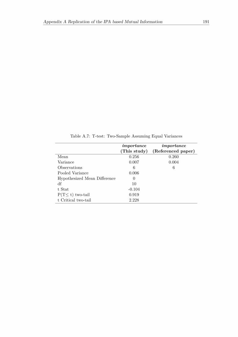
Appendix A Replication of the IPA based Mutual Information 191
Table A.7: T-test: Two-Sample Assuming Equal Variances
importance importance(This study) (Referenced paper)
Mean 0.256 0.260Variance 0.007 0.004Observations 6 6Pooled Variance 0.006Hypothesized Mean Difference 0df 10t Stat -0.104P(T≤ t) two-tail 0.919t Critical two-tail 2.228


Appendix B
Comparative Analysis ofClassification Algorithms usingWEKA
The main goal of this experiment is to verify that WEKA is installed and configuredcorrectly so it can be used for further experiments. The paper published by Rahmanand Afroz (2013) is selected as the referenced paper because this paper conducts thecomparison of various classifiers using WEKA on the UCI Machine Learning Repositorydatasets. Additionally, two classifiers used in Rahman and Afroz (2013) are similar tothe classifiers to be used in this research namely BPNN and BNs. More detail regardingdataset, tool, methodology and result will be described in next sections.
B.1 Dataset and Tool
Rahman and Afroz (2013) focus on the analysis of diabetes data and compare perfor-mance of different classification techniques in three data mining tools named WEKA,TANAGRA and MATLAB. Therefore, WEKA 3.6.10 and Pima Indians Diabetes, oneof the UCI Machine Learning Repository datasets 1, are selected to conduct the experi-ment.
The Pima Indians Diabetes dataset contains personal data (e.g., age, number of timespregnant) and the results of medical examinations (e.g., blood pressure, body massindex) which are the input attributes and the diagnostic of diabetes is an output attributewhich has two possible values (0 or 1) indicated that diabetes test is negative or positive.The details of this dataset are shown in Table B.1.
1http://archive.ics.uci.edu/ml/datasets.html
193

194 Appendix B Comparative Analysis of Classification Algorithms using WEKA
Table B.1: Detail of Pima Indians Diabetes Dataset
Numberof
Instances
Number ofAttributes
Numberof Classes
Attribute Type Missingattributesvalues
768 9 2 Integer, Real None
B.2 Methodology
In this section, the classifiers in the experiment are specified with their parameter setting.Additionally, the evaluation method and the performance metric are also specified inorder to measure the performance of each classifiers.
• ClassifiersThree classifiers in WEKA namely J48graft, Multilayer perceptron (MLP), andBayesNet are selected from five classifiers used in Rahman and Afroz’s paper.Default values of parameter are assigned to all parameters of each classifier asshown in Table B.2. Table B.2 also shows that all parameters of classifiers in thisstudy have been assigned similarly to the parameters of classifiers described inRahman and Afroz (2013).
Table B.2: Detail of Classifiers
Classifier Name This study Rahman and Afroz (2013)(Default value of WEKA)
J48graft confidenceFactor = 0.25 confidenceFactor = 0.25minNumObj = 2 minNumObj = 2subtreeRaising = True subtreeRaising = Trueunpruned = False unpruned = False
MLP learningRate = 0.3 learningRate = 0.3/0.15momentum = 0.2 momentum = 0.2randomSeed = 0 randomSeed = 0validationThreshold = 20 validationThreshold = 20number of Epochs = 500 number of Epochs = 500hiddenLayers = a
BayesNet estimator =SimpleEstimator estimator =SimpleEstimatorsearch algorithm = K2 search algorithm = K2ADTree = false ADTree = false
• Evaluation methodThe evaluation is conducted both in training and testing phase. In the trainingphase, the whole dataset is used as training and testing data. In the testing phase,Rahman and Afroz (2013) apply the Percentage Split (also called Holdout method)mode. In more detail, the 66% data is used for training and the remaining data isfor testing purposes therefore 507 instances are treated as training data and 261instances are treated as testing data. Since the goal of this study is to compare

Appendix B Comparative Analysis of Classification Algorithms using WEKA 195
performance with the result published in Rahman and Afroz (2013), the PercentageSplit is also used as test mode in this study with the option “preserve order for% split” to ensure that WEKA is randomly selected the same set of training andtesting data used in (Rahman and Afroz, 2013).
• Performance metricsAccuracy measured as percentage of correctly classified instances is used to evalu-ate performance of classifiers on training and testing data. Besides, others perfor-mance metrics derived from the confusion matrix like True-Positive Rate (TP rate),False-Positive rate (FP rate), and Precision, Recall, F-measure and ROC area arealso used to measure performance of classifiers on training and testing data. Thoseset of performance metrics are also used in Rahman and Afroz (2013), thus theycan use to compare the classifiers’ result of this study and Rahman and Afroz(2013).
B.3 Result
After the three classifiers are applied on Diabetes dataset in training and testing phase,their performances are measured regarding metrics described in the previous section andreported in Table B.3, Table B.4 and Table B.5.
Table B.3: Accuracy of different classifiers
Classifier Phase Accuracy (%) Accuracy (%) ofof this study Rahman and Afroz (2013)
J48graft Train 84.11 84.11Test 78.54 78.54
MLP Train 80.60 80.60Test 77.78 77.78
BayesNet Train 78.26 78.26Test 79.69 79.69
Table B.4: Different performance metrics in training phase
Metrics Classifiers of this study Classifiers ofRahman and Afroz (2013)
J48graft MLP BayesNet J48graft MLP BayesNetTP rate 0.841 0.806 0.783 0.841 0.806 0.783FP rate 0.241 0.191 0.26 0.241 0.191 0.26Precision 0.842 0.819 0.783 0.842 0.819 0.783Recall 0.841 0.806 0.783 0.841 0.806 0.783F-measure 0.836 0.809 0.783 0.836 0.809 0.783ROC area 0.888 0.872 0.851 0.888 0.872 0.851
The results from Table B.3 show that the accuracy of this study is similar to accuracypublished by Rahman and Afroz (2013) for all classifiers. Besides the accuracy, the

196 Appendix B Comparative Analysis of Classification Algorithms using WEKA
Table B.5: Different performance metrics in testing phase
Metrics Classifiers of this study Classifiers ofRahman and Afroz (2013)
J48graft MLP BayesNet J48graft MLP BayesNetTP rate 0.785 0.778 0.797 0.785 0.778 0.797FP rate 0.189 0.306 0.253 0.189 0.306 0.253Precision 0.816 0.774 0.799 0.816 0.774 0.799Recall 0.785 0.778 0.797 0.785 0.778 0.797F-measure 0.792 0.776 0.798 0.792 0.776 0.798ROC area 0.803 0.813 0.848 0.803 0.813 0.848
results of this study measured by other performance metrics such as True-Positive Rate,False-Positive Rate, Precision, Recall, F-Measure, and ROC Area are similar to theresults published by Rahman and Afroz (2013) as shown in Table B.4 and Table B.5.Based on these comparison results, it can be concluded that WEKA 3.6.10 is installedand configured correctly. Thus, this tool can be used for further data analysis forconducting IPA for SWOT analysis.

Appendix C
Assumption checking of themultiple linear regressions on 3datasets
To ensure that the result of MLR is valid several assumptions of MLR such as normality,linearity were tested. Assumption testing result for each dataset were summarized inTable C.1 and explained in the following sections.
Table C.1: Summary of assumption checking of MLR on 3 datasets
Assumptions DatasetA B C
Normality of residual X (2)× XLinearity X X XHomoscedasticity of residual (1)× (1)× XIndependence of residual X X XMulticollinearity X X X
With regard to Table C.1, a symbol X indicates that the assumption was met and a sym-bol × indicates that the assumption was violated. According to the table it shows thatthree assumptions which are linearity, independence of residual, and no multicollinearitywere met across three datasets. Whereas the other two assumptions: normality and ho-moscedasticity of residual were not met across three datasets. However, no further stepswere performed to correct these assumptions and the rationales to support this decisionare: (1) the regression is fairly robust to violation of homoscedasticity of residual. Besideviolation of this assumption does not affect the regression coefficients which were themain focus of this study(Keith, 2014) and (2) the deviation from normality of residualstested on dataset B was not the case to be concerned since the impact of departure fromzero kurtosis is diminished in reasonably large sample (200+ cases: Tabachnick et al.(2001)).
197

198 Appendix C Assumption checking of the multiple linear regressions on 3 datasets
C.1 Assumption checking of the multiple linear regressionson dataset A
Assumption 1: Normally distributed residual
The assumption of normality was visually tested by observing the histogram andnormal P-P plot of the standardized residual. Figure C.1 showed that the his-togram of residual appeared to look like a bell and the normal P-P plot wasapproximately a straight line, then it is plausible that the residual was normallydistributed.
(a) Histogram plot of residual (b) Normality plot of residual
Figure C.1: Histogram and normality plots of residual (dataset A)
Consistent with the histogram and normality plot, the skew and kurtosis of un-standardized residual shown in Table C.2 were fell within a reasonable range toaccept that data is reasonably close to normal which is −1.0 to +1.0 (George andMallery, 2003).
Table C.2: Descriptive statistic of unstandardized residual (dataset A)
N Mean Std. Skewness KurtosisDeviation Statistic Std. Error Statistic Std. Error
UnstandardizedResidual
264 0.000 0.7769 -0.533 0.15 1.032 0.299
Assumption 2: Linear relationship between independent and dependent variables
To check linearity assumption, a scatterplot of the standardized residual and stan-dardized predicted value was drawn. The residual plot for predicted values ofan outcome variable (Satisfaction) against the residuals (see Figure C.2) showedthat the dots are not constantly spread over the horizontal line; however, there

Appendix C Assumption checking of the multiple linear regressions on 3 datasets 199
is no sign of any curve pattern. Therefore, it cannot conclude that the linearityassumption was violated.
Figure C.2: Scatterplot of residual for the relationship between six independentvariables and the Satisfaction (dataset A)
Non-linear relationships can also be detected by looking at the partial regressionplots which are the scatterplots of the residuals of the outcome variable versusindividual independent variables. All partial regression plots (Figure C.3) showeda fairly random pattern and a positive relationship to Satisfaction which indicatedthe presence of linearity.
Apart from scatterplot and partial regression plot, it is useful to draw the scatter-plot of the outcome variable against each independent variable for the examinationof linearity. These scatterplots were drawn along with the curve fit of the linearmodel and non-linear models including: quadratic and cubic (see Figure C.4). Thecurve fit lines for each model of all scatterplots are appeared to be similar whichindicated that the linear model is fit to the data. However, the curve fit linesfor the non-linear models of the two independent variables named Equipment andTermCond are slightly different from that of the linear model.
To confirm the result of the graphical methods for evaluating linearity, for eachindependent variable the R-square of the four models are statistically comparedthrough the test of equality of several independent correlation coefficients (r).Regarding a rule of thumb, a relationship is linear if the difference between thelinear correlation coefficient (r) and the non-linear correlation coefficient is notsignificantly different.
Table C.3 - C.8 show the model summary of linear/non-linear function of eachindependent variable against the Satisfaction associated to the scatterplots shownin Figure C.4. Given R-square from Table C.3 - C.8, the test for equality of severalindependent correlation coefficients was conducted following an approach described

200 Appendix C Assumption checking of the multiple linear regressions on 3 datasets
(a) Partial regression plot of Equipment against Sat-isfaction
(b) Partial regression plot of SaleSup against Satis-faction
(c) Partial regression plot of TechSup against Satis-faction
(d) Partial regression plot of Supplier against Satis-faction
(e) Partial regression plot of AdminSup against Sat-isfaction
(f) Partial regression plot of TermCond against Sat-isfaction
Figure C.3: Partial regression plots of each independent variable against Satis-faction (dataset A)
in Kenny (1987). Then, the result of the test for equality of several independentcorrelation coefficients across six independent variables is reported in Table C.9.
Table C.9 shows that there is no significant difference among correlations of themodels for each independent variable. Therefore, it’s reasonable to conclude that

Appendix C Assumption checking of the multiple linear regressions on 3 datasets 201
Table C.3: Model summary corresponded to the scatterplot of Equipment versusSatisfaction
Equation Model SummaryR Square F df1 df2 p-value
Linear 0.155 48.068 1 262 0.000Quadratic 0.204 33.353 2 261 0.000Cubic 0.276 33.070 3 260 0.000
Table C.4: Model summary corresponded to the scatterplot of SaleSup versusSatisfaction
Equation Model SummaryR Square F df1 df2 p-value
Linear 0.065 18.269 1 262 0.000Quadratic 0.073 10.304 2 261 0.000Cubic 0.121 11.976 3 260 0.000
Table C.5: Model summary corresponded to the scatterplot of TechSup versusSatisfaction
Equation Model SummaryR Square F df1 df2 p-value
Linear 0.312 118.656 1 262 0.000Quadratic 0.313 59.561 2 261 0.000Cubic 0.317 40.184 3 260 0.000
Table C.6: Model summary corresponded to the scatterplot of Supplier versusSatisfaction
Equation Model SummaryR Square F df1 df2 p-value
Linear 0.136 41.137 1 262 0.000Quadratic 0.165 25.776 2 261 0.000Cubic 0.175 18.337 3 260 0.000
Table C.7: Model summary corresponded to the scatterplot of AdminSup versusSatisfaction
Equation Model SummaryR Square F df1 df2 p-value
Linear 0.042 11.403 1 262 0.001Quadratic 0.052 7.111 2 261 0.001Cubic 0.094 8.96 3 260 0.000
Table C.8: Model summary corresponded to the scatterplot of TermCond versusSatisfaction
Equation Model SummaryR Square F df1 df2 p-value
Linear 0.163 51.025 1 262 0.000Quadratic 0.183 29.17 2 261 0.000Cubic 0.236 26.705 3 260 0.000

202 Appendix C Assumption checking of the multiple linear regressions on 3 datasets
(a) Curve estimation of Equipment against Satisfac-tion
(b) Curve estimation of SaleSup against Satisfaction
(c) Curve estimation of TechSup against Satisfaction (d) Curve estimation of Supplier against Satisfaction
(e) Curve estimation of AdminSup against Satisfac-tion
(f) Curve estimation of TermCond against Satisfac-tion
Figure C.4: Scatterplot with model curve fit of each independent variableagainst Satisfaction (dataset A)
the relationship between each independent variable and the Satisfaction is linear.

Appendix C Assumption checking of the multiple linear regressions on 3 datasets 203
Table C.9: Chi-square statistic for the difference test of several independentcorrelations (dataset A)
Independent variable χ2 df p-value EqualityEquipment 3.693 2 0.158 YesSaleSup 1.576 2 0.455 YesTechSup 0.006 2 0.997 YesSupplier 0.487 2 0.784 YesAdminSup 1.706 2 0.426 YesTermCond 1.455 2 0.483 Yes
Assumption 3: Homoscedasticity of residuals
The assumption is that the residuals at each level of the dependent variables hadthe same variance. There are graphical and non-graphical methods for checkinghomoscedasticity. For the graphical method, the scatterplot of the standardizedresidual and standardized predicted value as shown in Figure C.2 was reobserved.Although the dots were not constantly spread over the horizontal line, a funnelshaped pattern did not appear. It may be inferred that this assumption was met.
A non-graphical method using Breusch-Pagan test suggested that the variance ofthe residuals is not homogenous. The null hypothesis of Breusch-Pagan test ishomoscedasticity. In this case, the null hypothesis is rejected (BP =23.95, df = 1,p-value =0.000).
Note that steps for conducting Breusch-Pagan test using SPSS is referred to Pryce(2002) and the validity of this test is depended on the normality of residual. Thehistogram and normality plot of residuals shown in Figure C.1 suggested that theresiduals are fairly normal; therefore, the test result was reliable.
Even though this assumption was not met, further steps were not performed tocorrect this assumption because the regression is fairly robust to violation of thisassumption. Beside violation of this assumption does not affect the regressioncoefficients which were the main focus of this study (Keith, 2014).
Assumption 4: Independence of residual (error)
The assumption is that the error is not correlated with any independent variables.The independence of residuals was checked through the Durbin-Watson statistic ofthe regression model. A conventionally acceptable range of this statistic is 1 - 3 inwhich the value close to 2 indicates no autocorrelation (Field, 2009). In this case,Durbin-Watson statistic was 1.99 indicated the lack of autocorrelation thereby theassumption was met.
Assumption 5: Multicollinearity
Under the assumption of no multicollinearity, the independent variables are notclosely linearly related to each other. The degree of multicollinearity can be de-tected by inspecting the VIF statistic provided by SPSS. A VIF of 1 means that

204 Appendix C Assumption checking of the multiple linear regressions on 3 datasets
there is no correlation among the independent variables while VIF higher than 1indicates a presence of multicollinearity among them. As a rule of thumb, VIFhigher than 10 indicates the sign of serious multicollinearity (Field, 2009). TheVIF for each independent variable was greater than 1 but lower than 10 (see Ta-ble C.10) hence it’s can conclude that multicollinearity was present but there isno sign of serious multicollinearity which requires correction (such as removingredundant variables) within the dataset A.
Table C.10: Collinearity Statistics (VIF) of six independent variables (datasetA)
Independent variable Collinearity Statistics (VIF )Equipment 1.212SaleSup 1.188TechSup 1.251Supplier 1.187AdminSup 1.157TermCond 1.348
C.2 Assumption checking of the multiple linear regressionson dataset B
Assumption 1: Normally distributed residual
The assumption of normality was visually tested by observing the histogram andnormal P-P plot of the standardized residual. Figure C.5 showed that the his-togram of residual appeared to look like a bell but rather peak and the normalP-P plot was approximately a straight line, then it is plausible that the residualwas normally distributed.
In addition to the histogram and normality plot, the skew and kurtosis of unstan-dardized residual were also observed to check the normality of residuals. Table C.11 showed that only the skew was fell within reasonable range to accept that datais reasonably close to normal which is −1.0 to +1.0 (George and Mallery, 2003).Although the kurtosis was higher than 1.0, the impact of departure from zerokurtosis is diminished in reasonably large sample (200+ cases) (Tabachnick et al.,2001). Thus, the deviation from normality of residuals was not the case to beconcerned.
Table C.11: Descriptive statistic of unstandardized residual (dataset B)
N Mean Std. Skewness KurtosisDeviation Statistic Std. Error Statistic Std. Error
UnstandardizedResidual
4500 0.000 0.504 -0.273 0.037 2.88 0.073

Appendix C Assumption checking of the multiple linear regressions on 3 datasets 205
(a) Histogram plot of residual (b) Normality plot of residual
Figure C.5: Histogram and normality plots of residual (dataset B)
Assumption 2: Linear relationship between independent and dependent variables
To check linearity assumption, a scatterplot of the standardized residual and stan-dardized predicted value was drawn. The residual plot for predicted values of anoutcome variable (V56) against the residuals (see Figure C.6) showed that the dotsare not constantly spread over the horizontal line; however, there is no sign of anycurve pattern. Therefore, it cannot conclude that the linearity assumption wasviolated.
Figure C.6: Scatterplot of residual for the relationship between 13 independentvariables and the V56 (dataset B)
Non-linear relationships can also be detected by looking at the partial regression

206 Appendix C Assumption checking of the multiple linear regressions on 3 datasets
plots which are the scatterplots of the residuals of the outcome variable versus in-dividual independent variables (V42 - V54). All partial regression plots (Figure C.7 - C.8) showed a fairly random pattern to V56 which may indicate the presenceof linearity.
(a) Partial regression plot of V42 against V56 (b) Partial regression plot of V43 against V56
(c) Partial regression plot of V44 against V56 (d) Partial regression plot of V45 against V56
(e) Partial regression plot of V46 against V56 (f) Partial regression plot of V47 against V56
Figure C.7: Partial regression plots of independent variable V42-V47 againstV56 (dataset B)
Apart from scatterplot and partial regression plot, it is useful to draw the scatter-plot of the outcome variable against each independent variable for the examinationof linearity. These scatterplots were drawn along with the curve fit of the linearmodel and non-linear models including: logarithmic, quadratic and cubic (see Fig-ure C.9 - C.10). For each variable, the curve fit lines for linear model are appeared

Appendix C Assumption checking of the multiple linear regressions on 3 datasets 207
to be similar to that of quadratic and cubic model in the other word only the curvefit lines for logarithmic model are slightly different from the others.
Since the linearity cannot be confirmed using these graphs, the R-square of thefour models for each independent variable shown in Table C.12 - C.24 are statis-tically compared through the test of equality for several independent correlationcoefficients (r). The test for equality of several independent correlation coefficientswas conducted following to an approach described in Kenny (1987). Then, the re-sult of the test for equality of several independent correlation coefficients across13 independent variables is reported in Table C.25.
Table C.12: Model summary corresponded to the scatterplot of V42 versus V56
Equation Model SummaryR Square F df1 df2 p-value
Linear 0.197 1106.156 1 4498 0.000Logarithmic 0.186 1030.152 1 4498 0.000Quadratic 0.199 557.093 2 4497 0.000Cubic 0.199 371.625 3 4496 0.000
Table C.13: Model summary corresponded to the scatterplot of V43 versus V56
Equation Model SummaryR Square F df1 df2 p-value
Linear 0.246 1468.859 1 4498 0.000Logarithmic 0.232 1356.8 1 4498 0.000Quadratic 0.247 739.37 2 4497 0.000Cubic 0.247 492.836 3 4496 0.000
Table C.14: Model summary corresponded to the scatterplot of V44 versus V56
Equation Model SummaryR Square F df1 df2 p-value
Linear 0.293 1866.597 1 4498 0.000Logarithmic 0.281 1758.288 1 4498 0.000Quadratic 0.295 941.726 2 4497 0.000Cubic 0.296 631.63 3 4496 0.000
Table C.15: Model summary corresponded to the scatterplot of V45 versus V56
Equation Model SummaryR Square F df1 df2 p-value
Linear 0.336 2280.634 1 4498 0.000Logarithmic 0.332 2234.325 1 4498 0.000Quadratic 0.343 1174.4 2 4497 0.000Cubic 0.344 785.072 3 4496 0.000
Table C.25 shows that there is no significant difference among correlations of themodels for each independent variable. Therefore, it’s reasonable to conclude that
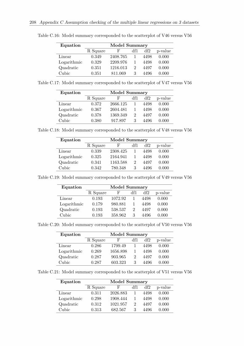
208 Appendix C Assumption checking of the multiple linear regressions on 3 datasets
Table C.16: Model summary corresponded to the scatterplot of V46 versus V56
Equation Model SummaryR Square F df1 df2 p-value
Linear 0.349 2408.765 1 4498 0.000Logarithmic 0.329 2209.976 1 4498 0.000Quadratic 0.351 1216.013 2 4497 0.000Cubic 0.351 811.069 3 4496 0.000
Table C.17: Model summary corresponded to the scatterplot of V47 versus V56
Equation Model SummaryR Square F df1 df2 p-value
Linear 0.372 2666.125 1 4498 0.000Logarithmic 0.367 2604.481 1 4498 0.000Quadratic 0.378 1369.349 2 4497 0.000Cubic 0.380 917.897 3 4496 0.000
Table C.18: Model summary corresponded to the scatterplot of V48 versus V56
Equation Model SummaryR Square F df1 df2 p-value
Linear 0.339 2308.425 1 4498 0.000Logarithmic 0.325 2164.941 1 4498 0.000Quadratic 0.341 1163.588 2 4497 0.000Cubic 0.342 780.348 3 4496 0.000
Table C.19: Model summary corresponded to the scatterplot of V49 versus V56
Equation Model SummaryR Square F df1 df2 p-value
Linear 0.193 1072.92 1 4498 0.000Logarithmic 0.179 980.881 1 4498 0.000Quadratic 0.193 538.537 2 4497 0.000Cubic 0.193 358.962 3 4496 0.000
Table C.20: Model summary corresponded to the scatterplot of V50 versus V56
Equation Model SummaryR Square F df1 df2 p-value
Linear 0.286 1799.49 1 4498 0.000Logarithmic 0.269 1656.898 1 4498 0.000Quadratic 0.287 903.965 2 4497 0.000Cubic 0.287 603.323 3 4496 0.000
Table C.21: Model summary corresponded to the scatterplot of V51 versus V56
Equation Model SummaryR Square F df1 df2 p-value
Linear 0.311 2026.883 1 4498 0.000Logarithmic 0.298 1908.444 1 4498 0.000Quadratic 0.312 1021.957 2 4497 0.000Cubic 0.313 682.567 3 4496 0.000

Appendix C Assumption checking of the multiple linear regressions on 3 datasets 209
Table C.22: Model summary corresponded to the scatterplot of V52 versus V56
Equation Model SummaryR Square F df1 df2 p-value
Linear 0.348 2399.94 1 4498 0.000Logarithmic 0.343 2349.145 1 4498 0.000Quadratic 0.354 1233.484 2 4497 0.000Cubic 0.355 823.322 3 4496 0.000
Table C.23: Model summary corresponded to the scatterplot of V53 versus V56
Equation Model SummaryR Square F df1 df2 p-value
Linear 0.326 2171.462 1 4498 0.000Logarithmic 0.315 2065.275 1 4498 0.000Quadratic 0.327 1094.153 2 4497 0.000Cubic 0.330 737.211 3 4496 0.000
Table C.24: Model summary corresponded to the scatterplot of V54 versus V56
Equation Model SummaryR Square F df1 df2 p-value
Linear 0.337 2285.828 1 4498 0.000Logarithmic 0.334 2255.471 1 4498 0.000Quadratic 0.342 1170.232 2 4497 0.000Cubic 0.344 787.14 3 4496 0.000
Table C.25: Chi-square statistic for the difference test of several independentcorrelations (dataset B)
Independent variable χ2 df p-value EqualityV42 1.046 3 0.790 YesV43 1.315 3 0.725 YesV44 1.115 3 0.774 YesV45 0.750 3 0.861 YesV46 2.612 3 0.455 YesV47 0.803 3 0.849 YesV48 1.433 3 0.698 YesV49 1.341 3 0.719 YesV50 1.822 3 0.610 YesV51 1.137 3 0.768 YesV52 0.715 3 0.870 YesV53 0.980 3 0.806 YesV54 0.476 3 0.924 Yes

210 Appendix C Assumption checking of the multiple linear regressions on 3 datasets
the relationship between each independent variable and the V56 is linear.
Assumption 3: Homoscedasticity of residuals
The assumption is that the residuals at each level of the dependent variables hadthe same variance. There are graphical and non-graphical methods for checkinghomoscedasticity. For the graphical method, the scatterplot of the standardizedresidual and standardized predicted value as shown in Figure C.6 was reobserved.Although the dots were spread out more at upper level of standardized predictedvalue than at lower level, a funnel shaped pattern did not appear. It may beinferred that heteroscedasticity was not present.
In contrast with the graphical method, a non-graphical method using Breusch-Pagan test suggested that the variance of the residuals is not homogenous. Thenull hypothesis of Breusch-Pagan test is homoscedasticity. In this case, the nullhypothesis is rejected (BP =173.09, df = 1, p-value = 0.000).
Note that steps for conducting Breusch-Pagan test using SPSS is referred to Pryce(2002) and the validity of this test is depended on the normality of residual. Thehistogram and normality plot of residuals shown in Figure C.5 suggested that theresiduals are fairly normal; therefore, the test result was reliable.
Even though this assumption was not met, further steps were not performed tocorrect this assumption because the regression is fairly robust to violation of thisassumption. Beside violation of this assumption does not affect the regressioncoefficients which were the main focus of this study (Keith, 2014).
Assumption 4: Independence of residual (error)
The assumption is that the error is not correlated with any independent variables.The independence of residuals was checked through the Durbin-Watson statistic ofthe regression model. A conventionally acceptable range of this statistic is 1 - 3 inwhich the value close to 2 indicates no autocorrelation (Field, 2009). In this case,Durbin-Watson statistic was 1.96 indicated the lack of autocorrelation thereby theassumption was met.
Assumption 5: Multicollinearity
Under the assumption of no multicollinearity, the independent variables are notclosely linearly related to each other. The degree of multicollinearity can be de-tected by inspecting the VIF statistic provided by SPSS. A VIF of 1 means thatthere is no correlation among the independent variables while VIF higher than 1indicates a presence of multicollinearity among them. As a rule of thumb, VIFhigher than 10 indicates the sign of serious multicollinearity (Field, 2009). TheVIF for each independent variable was greater than 1 but lower than 10 (see Ta-ble C.26) hence it’s can conclude that multicollinearity was present but there is

Appendix C Assumption checking of the multiple linear regressions on 3 datasets 211
no sign of serious multicollinearity which requires correction (such as removingredundant variables) within the dataset B.
Table C.26: Collinearity Statistics (VIF) of 13 independent variables (datasetB)
Independent variable Collinearity Statistics (VIF )V42 4.294V43 5.454V44 4.244V45 4.719V46 5.114V47 5.921V48 4.398V49 3.668V50 5.230V51 4.539V52 5.381V53 5.470V54 4.191
C.3 Assumption checking of the multiple linear regressionson dataset C
Assumption 1: Normally distributed residual
The assumption of normality was visually tested by observing the histogram andnormal P-P plot of the standardized residual. Figure C.11 showed that the his-togram of residual appeared to look like a bell and the normal P-P plot wasapproximately a straight line, then it is plausible that the residual was normallydistributed.
Consistent with the histogram and normality plot, the skew and kurtosis of un-standardized residual shown in Table C.27 were fell within a reasonable range toaccept that data is reasonably close to normal which is −1.0 to +1.0 (George andMallery, 2003).
Table C.27: Descriptive statistic of unstandardized residual (dataset C)
N Mean Std. Skewness KurtosisDeviation Statistic Std. Error Statistic Std. Error
UnstandardizedResidual
155 0.000 0.3717 0.162 0.195 0.603 0.387
Assumption 2: Linear relationship between independent and dependent variables
To check linearity assumption, a scatterplot of the standardized residual and stan-dardized predicted value was drawn. The residual plot for predicted values of an

212 Appendix C Assumption checking of the multiple linear regressions on 3 datasets
outcome variable (OCS student) against the residuals (see Figure C.12) showedthat the dots are not constantly spread over the horizontal line; however, thereis no sign of any curve pattern. Therefore, it cannot conclude that the linearityassumption was violated.
Non-linear relationships can also be detected by looking at the partial regressionplots which are the scatterplots of the residuals of the outcome variable versusindividual independent variables. All partial regression plots (Figure C.13) showeda fairly random pattern and a positive relationship to OCS student which indicatedthe presence of linearity.
Apart from scatterplot and partial regression plot, it is useful to draw the scatter-plot of the outcome variable against each independent variable for the examinationof linearity. These scatterplots were drawn along with the curve fit of the linearmodel and non-linear models including: quadratic and cubic (see Figure C.14).The curve fit lines for each model of all scatterplots are appeared to be similarwhich indicated that the linear model is fit to the data. However, the curve fitlines for the non-linear models of the two independent variables named Teachingand CompFac are slightly different from that of the linear model.
To confirm the result of the graphical methods for evaluating linearity, for eachindependent variable the R-square of the four models for each independent variableshown in Table C.28 - C.33 are statistically compared through the test of equalityof several independent correlation coefficients (r). The test for equality of severalindependent correlation coefficients was conducted following an approach describedin Kenny (1987). Then, the result of the test for equality of several independentcorrelation coefficients across six independent variables is reported in Table C.34.
Table C.28: Model summary corresponded to the scatterplot of Teacher versusOCS student
Equation Model SummaryR Square F df1 df2 p-value
Linear 0.319 71.704 1 153 0.000Logarithmic 0.311 68.988 1 153 0.000Quadratic 0.319 35.674 2 152 0.000Cubic 0.319 35.674 2 152 0.000
Table C.29: Model summary corresponded to the scatterplot of Teaching versusOCS student
Equation Model SummaryR Square F df1 df2 p-value
Linear 0.413 107.439 1 153 0.000Logarithmic 0.378 93.056 1 153 0.000Quadratic 0.433 57.955 2 152 0.000Cubic 0.429 57.076 2 152 0.000
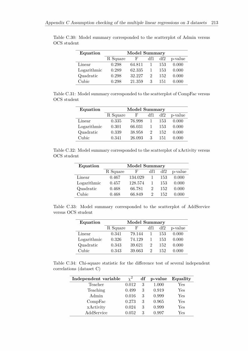
Appendix C Assumption checking of the multiple linear regressions on 3 datasets 213
Table C.30: Model summary corresponded to the scatterplot of Admin versusOCS student
Equation Model SummaryR Square F df1 df2 p-value
Linear 0.298 64.811 1 153 0.000Logarithmic 0.289 62.335 1 153 0.000Quadratic 0.298 32.227 2 152 0.000Cubic 0.298 21.359 3 151 0.000
Table C.31: Model summary corresponded to the scatterplot of CompFac versusOCS student
Equation Model SummaryR Square F df1 df2 p-value
Linear 0.335 76.998 1 153 0.000Logarithmic 0.301 66.031 1 153 0.000Quadratic 0.339 38.958 2 152 0.000Cubic 0.341 26.093 3 151 0.000
Table C.32: Model summary corresponded to the scatterplot of xActivity versusOCS student
Equation Model SummaryR Square F df1 df2 p-value
Linear 0.467 134.029 1 153 0.000Logarithmic 0.457 128.574 1 153 0.000Quadratic 0.468 66.781 2 152 0.000Cubic 0.468 66.849 2 152 0.000
Table C.33: Model summary corresponded to the scatterplot of AddServiceversus OCS student
Equation Model SummaryR Square F df1 df2 p-value
Linear 0.341 79.144 1 153 0.000Logarithmic 0.326 74.129 1 153 0.000Quadratic 0.343 39.621 2 152 0.000Cubic 0.343 39.663 2 152 0.000
Table C.34: Chi-square statistic for the difference test of several independentcorrelations (dataset C)
Independent variable χ2 df p-value EqualityTeacher 0.012 3 1.000 YesTeaching 0.499 3 0.919 YesAdmin 0.016 3 0.999 Yes
CompFac 0.273 3 0.965 YesxActivity 0.024 3 0.999 YesAddService 0.052 3 0.997 Yes

214 Appendix C Assumption checking of the multiple linear regressions on 3 datasets
Table C.34 shows that there is no significant difference among correlations of themodels for each independent variable. Therefore, it’s reasonable to conclude thatthe relationship between each independent variable and the OCS student is linear.
Assumption 3: Homoscedasticity of residuals
The assumption is that the residuals at each level of the dependent variables hadthe same variance. There are graphical and non-graphical methods for checkinghomoscedasticity. For the graphical method, the scatterplot of the standardizedresidual and standardized predicted value as shown in Figure C.12 was reobserved.Although the dots were not constantly spread over the horizontal line, a funnelshaped pattern did not appears. It may be inferred that this assumption was met.
Consistent with the graphical method, a non-graphical method using Breusch-Pagan test suggested that the variance of the residuals is homogenous. The nullhypothesis of Breusch-Pagan test is homoscedasticity. In this case, the null hy-pothesis is retained (BP = 0.742, df = 1, p-value = 0.389).
Note that steps for conducting Breusch-Pagan test using SPSS is referred to Pryce(2002) and the validity of this test is depended on the normality of residual. Thehistogram and normality plot of residuals shown in Figure C.11 suggested that theresiduals are fairly normal; therefore, the test result was reliable.
Assumption 4: Independence of residual (error)
The assumption is that the error is not correlated with any independent variables.The independence of residuals was checked through the Durbin-Watson statistic ofthe regression model. A conventionally acceptable range of this statistic is 1 - 3 inwhich the value close to 2 indicates no autocorrelation (Field, 2009). In this case,Durbin-Watson statistic was 2.02 indicated the lack of autocorrelation thereby theassumption was met.
Assumption 5: Multicollinearity
Under the assumption of no multicollinearity, the independent variables are notclosely linearly related to each other. The degree of multicollinearity can be de-tected by inspecting the VIF statistic provided by SPSS. A VIF of 1 means thatthere is no correlation among the independent variables while VIF higher than 1indicates a presence of multicollinearity among them. As a rule of thumb, VIFhigher than 10 indicates the sign of serious multicollinearity (Field, 2009). TheVIF for each independent variable was greater than 1 but lower than 10 (see Ta-ble C.35) hence it’s can conclude that multicollinearity was present but there isno sign of serious multicollinearity which requires correction (such as removingredundant variables) within the dataset C.

Appendix C Assumption checking of the multiple linear regressions on 3 datasets 215
Table C.35: Collinearity Statistics (VIF) of six independent variables (datasetC)
Independent variable Collinearity Statistics (VIF )Teacher 1.635Teaching 2.058Admin 1.807CompFac 2.300XActivity 2.353AddService 2.193

216 Appendix C Assumption checking of the multiple linear regressions on 3 datasets
(a) Partial regression plot of V48 against V56 (b) Partial regression plot of V49 against V56
(c) Partial regression plot of V50 against V56 (d) Partial regression plot of V51 against V56
(e) Partial regression plot of V52 against V56 (f) Partial regression plot of V53 against V56
(g) Partial regression plot of V54 against V56
Figure C.8: Partial regression plots of independent variable V48-V54 againstV56 (dataset B)

Appendix C Assumption checking of the multiple linear regressions on 3 datasets 217
(a) Curve estimation of V42 against V56 (b) Curve estimation of V43 against V56
(c) Curve estimation of V44 against V56 (d) Curve estimation of V45 against V56
(e) Curve estimation of V46 against V56 (f) Curve estimation of V47 against V56
(g) Curve estimation of V48 against V56 (h) Curve estimation of V49 against V56
Figure C.9: Scatterplot with model curve fit of independent variable V42-V49against V56 (dataset B)

218 Appendix C Assumption checking of the multiple linear regressions on 3 datasets
(a) Curve estimation of V50 against V56 (b) Curve estimation of V51 against V56
(c) Curve estimation of V52 against V56 (d) Curve estimation of V53 against V56
(e) Curve estimation of V544 against V56
Figure C.10: Scatterplot with model curve fit of independent variable V50-V54against V56 (dataset B)

Appendix C Assumption checking of the multiple linear regressions on 3 datasets 219
(a) Histogram plot of residual (b) Normality plot of residual
Figure C.11: Histogram and normality plots of residual (dataset C)
Figure C.12: Scatterplot of residual for the relationship between six independentvariables and the OCS student (dataset C)

220 Appendix C Assumption checking of the multiple linear regressions on 3 datasets
(a) Partial regression plot of Teacher against OCSstudent
(b) Partial regression plot of Teaching against OCSstudent
(c) Partial regression plot of Admin against OCS stu-dent
(d) Partial regression plot of CompFac against OCSstudent
(e) Partial regression plot of xActivity against OCSstudent
(f) Partial regression plot of AddService against OCSstudent
Figure C.13: Partial regression plots of each independent variable against OCSstudent (dataset C)

Appendix C Assumption checking of the multiple linear regressions on 3 datasets 221
(a) Curve estimation of Teacher against OCS student (b) Curve estimation of Teaching against OCS stu-dent
(c) Curve estimation of Admin against OCS student (d) Curve estimation of CompFac against OCS stu-dent
(e) Curve estimation of xActivity against OCS stu-dent
(f) Curve estimation of AddService against OCS stu-dent
Figure C.14: Scatterplot with model curve fit of each independent variableagainst OCS student (dataset C)


Appendix D
Assumption checking of theordinal logistic regressions on 3datasets
To ensure that the result of OLR is valid one key assumption of OLR named proportionalodds (or the assumption of parallel lines in SPSS) was tested. The null hypothesis forthe test of proportional odds states that the corresponding regression coefficients in thelink function are the same across all categories of ordinal responses.
The assumption is retained in case that the p-value (or Sig.) is greater than 0.05,otherwise the assumption is rejected. Assumption testing results for each dataset weresummarized in Table D.1 and their detail was shown in Table D.2 - D.4.
Table D.1: Summary of assumption checking of OLR on 3 datasets
Assumptions DatasetA B C
Proportional odds X X ×
With regard to Table D.1, a symbol X indicate that the assumption was met and asymbol × indicate that the assumption was violated. According to the table it showsthat the assumption was met for the dataset A and dataset B, but the assumption wasviolate for the dataset C.
Even though the assumption of proportional odds was not met for the OLR modelon dataset C, the other models of OLR such as Partial proportional Odds(PPO) andProportional Odds With Partial Proportionality Constraints (POPPC) that relax theproportional odds assumption were not considered to use in this study. This is be-cause the PPO and POPPC are more complicated than proportional odds that used in
223

224 Appendix D Assumption checking of the ordinal logistic regressions on 3 datasets
this study. As suggested by Fullerton (2009) that researchers should trade-off betweenaccuracy and parsimony.
Table D.2: Test of proportional odds on dataset A
Model -2 Log Likelihood Chi-Square df Sig.Null Hypothesis 464.753General 463.545 1.208 24 1.000
Table D.3: Test of proportional odds on dataset B
Model -2 Log Likelihood Chi-Square df Sig.Null Hypothesis 0.000General 0.000 0.000 52 1.000
Table D.4: Test of proportional odds on dataset C
Model -2 Log Likelihood Chi-Square df Sig.Null Hypothesis 48.315General 0.000 48.315 6 0.000

Appendix E
Assigning number of hidden-layerneurons
Following to Maren, Harston, and Pap (1990) cited in Deng et al. (2008a) the boundof neurons in the first hidden layer was between 2N + 1 and O(N + 1), where N is thenumber of input neurons and O is the number of output neurons, the bound of numberhidden-layer neurons for each dataset is shown in Table E.1.
Table E.1: The bound of hidden-layer neurons
Dataset N BPNN(regression) BPNN(classification)O O(N+1) 2N+1 O 2N+1 O(N+1)
A 6 1 7 13 6 13 42B 13 1 14 27 6 27 84C 6 1 7 13 5 13 35
Regarding Table E.1, the bounds of hidden-layer neurons for BPNN (regression) are {7,13}, {14, 27} and {7, 13} for dataset A, B and C respectively. The bounds of hidden-layer neurons for BPNN (classification) are {13, 42}, {27, 84} and {13, 35} for datasetA, B and C respectively. In addition, several formulae for calculating number of hiddenlayers, shown in Table E.2, are also considered.
In order to determine the number of neurons in the hidden layer of the two BPNNstructure models, several configurations of hidden-layer neurons were trained on thetraining dataset. Then, statistical comparisons of the performance of BPNN trainedmodels were performed using Experimenter application in WEKA. Specifically, eachgiven BPNN model was tested using 10-fold cross validation repeated 10 times for smalldataset (dataset A and C), using percentage split for dataset B. Subsequently, the pairedT-test was conducted (with 5% significance level) to check the null hypothesis that themean difference of performance measures (e.g. accuracy) between the BPNN models iszero.
225
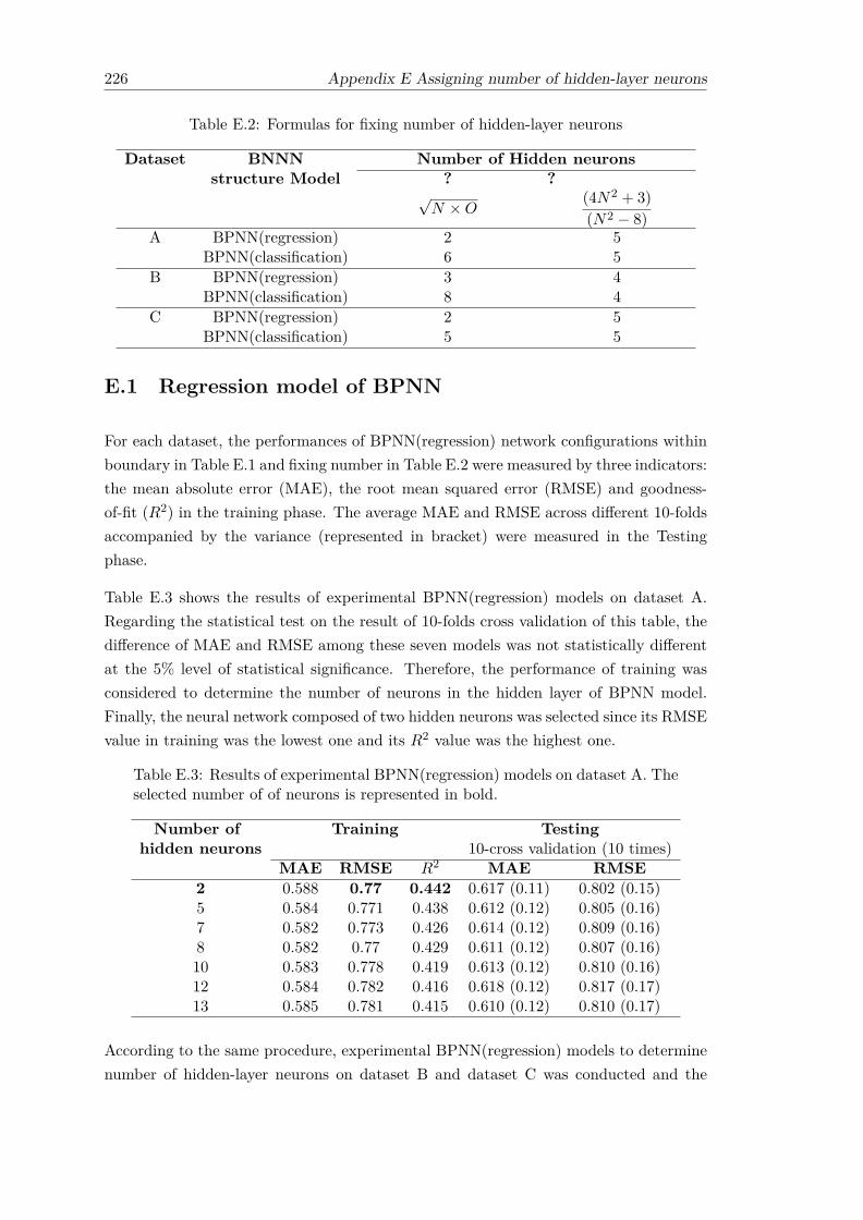
226 Appendix E Assigning number of hidden-layer neurons
Table E.2: Formulas for fixing number of hidden-layer neurons
Dataset BNNN Number of Hidden neuronsstructure Model ? ?
√N ×O
(4N2 + 3)
(N2 − 8)A BPNN(regression) 2 5
BPNN(classification) 6 5B BPNN(regression) 3 4
BPNN(classification) 8 4C BPNN(regression) 2 5
BPNN(classification) 5 5
E.1 Regression model of BPNN
For each dataset, the performances of BPNN(regression) network configurations withinboundary in Table E.1 and fixing number in Table E.2 were measured by three indicators:the mean absolute error (MAE), the root mean squared error (RMSE) and goodness-of-fit (R2) in the training phase. The average MAE and RMSE across different 10-foldsaccompanied by the variance (represented in bracket) were measured in the Testingphase.
Table E.3 shows the results of experimental BPNN(regression) models on dataset A.Regarding the statistical test on the result of 10-folds cross validation of this table, thedifference of MAE and RMSE among these seven models was not statistically differentat the 5% level of statistical significance. Therefore, the performance of training wasconsidered to determine the number of neurons in the hidden layer of BPNN model.Finally, the neural network composed of two hidden neurons was selected since its RMSEvalue in training was the lowest one and its R2 value was the highest one.
Table E.3: Results of experimental BPNN(regression) models on dataset A. Theselected number of of neurons is represented in bold.
Number of Training Testinghidden neurons 10-cross validation (10 times)
MAE RMSE R2 MAE RMSE2 0.588 0.77 0.442 0.617 (0.11) 0.802 (0.15)5 0.584 0.771 0.438 0.612 (0.12) 0.805 (0.16)7 0.582 0.773 0.426 0.614 (0.12) 0.809 (0.16)8 0.582 0.77 0.429 0.611 (0.12) 0.807 (0.16)10 0.583 0.778 0.419 0.613 (0.12) 0.810 (0.16)12 0.584 0.782 0.416 0.618 (0.12) 0.817 (0.17)13 0.585 0.781 0.415 0.610 (0.12) 0.810 (0.17)
According to the same procedure, experimental BPNN(regression) models to determinenumber of hidden-layer neurons on dataset B and dataset C was conducted and the

Appendix E Assigning number of hidden-layer neurons 227
results are shown in Table E.4 and Table E.5 respectively. Besides, the number of hidden-layer neurons within boundary and the number of hidden-layer neurons suggested bythe formulae in Table E.2, these two experimental BPNN(regression) models were alsoincluded number of hidden-layer neurons according to the WEKA option which are N,O, N+O and (N+O)/2, where N is the number of input neurons and O is the numberof output neurons.
Table E.4 shows the results of experimental BPNN(regression) models on dataset B.The performance of training among 10 models was about the same and there was nosignificantly difference of MAE and RMSE among the performance testing of percentagesplit of 10 models. Thus, the neural network composed of three hidden neurons wasselected since this model produced the lowest MAE and RMSE although it was notstatically different from other models.
Table E.4: Results of experimental BPNN(regression) models on dataset B. Theselected number of of neurons is represented in bold.
Number of Training Testinghidden neurons Percentage split (10 times)
MAE RMSE R2 MAE RMSE1 0.383 0.501 0.435 0.388(0.01) 0.507 (0.01)3 0.38 0.499 0.441 0.385 (0.01) 0.507 (0.01)4 0.38 0.499 0.441 0.385 (0.01) 0.508 (0.01)7 0.38 0.499 0.441 0.386 (0.01) 0.507 (0.01)13 0.38 0.499 0.44 0.387 (0.01) 0.507 (0.01)14 0.38 0.499 0.441 0.387 (0.01) 0.507 (0.01)15 0.38 0.500 0.440 0.387 (0.01) 0.507 (0.01)18 0.38 0.499 0.442 0.387 (0.01) 0.507 (0.01)21 0.38 0.499 0.441 0.387 (0.01) 0.507 (0.01)25 0.38 0.499 0.441 0.387 (0.01) 0.507 (0.01)
Regarding Table E.5, the model with 12 hidden neurons yielded similar performance intraining and testing as same as model with 13 hidden neurons, their MAE measuredthrough 10-folds cross validation of this model was statistically different at the 5% levelof statistical significance from other models with 1-3, 5-8 hidden-layer neuron(s). Bothmodels also yielded lowest MAE and highest R2 in training. Thus, either of them isqualified to be selected however considering the number of hidden neurons, the smallernumber of hidden neurons was preferable. Thereby, the neural network composed of 12hidden neurons was selected.
E.2 Classification model of BPNN
For the classification model of BPNN, networks with different number of hidden neuronswithin boundary in Table E.1 and fixing number in Table E.2, and number of hidden-layer neurons according to the WEKA option which are N, O, N+O and (N+O)/2

228 Appendix E Assigning number of hidden-layer neurons
Table E.5: Results of experimental BPNN(regression) models on dataset C. Theselected number of of neurons is represented in bold.
Number of Training Testinghidden neurons 10-cross validation (10 times)
MAE RMSE R2 MAE RMSE1 0.313 0.371 0.61 0.33(0.05) * 0.40(0.08) *2 0.311 0.37 0.613 0.33(0.05) * 0.39(0.08)3 0.31 0.369 0.614 0.33(0.05) * 0.39(0.08)5 0.31 0.369 0.614 0.33(0.05) * 0.39(0.08)6 0.308 0.368 0.616 0.33(0.05) * 0.39(0.08)7 0.309 0.369 0.615 0.33(0.05) * 0.39(0.08)8 0.307 0.368 0.616 0.32(0.05) * 0.39(0.08)10 0.308 0.368 0.616 0.32(0.05) 0.39(0.08)11 0.307 0.368 0.617 0.32(0.05) 0.39(0.08)12 0.306 0.368 0.617 0.32(0.05) 0.39(0.08)13 0.306 0.368 0.617 0.32(0.05) 0.39(0.08)
* Significantly difference with the neural network composed of 12 hidden neurons
were trained. Then, their performance was measured by three indicators: percentageof accuracy, RMSE and area under the Receiver Operating Characteristic (ROC) curve(AUC). For the testing phase average percentage accuracy, RMSE and AUC across dif-ferent evaluation 10 times accompanied by the variance are shown. For each dataset, theresults of experimental BPNN(classification) models are shown in Table E.6 - Table E.8.
The test of statistical significance on the result of 10-folds cross validation in TableE.6 shows that the RMSE and AUC of two models with five and six hidden neuronswere statistically different from other network structures at the 5% level of statisticalsignificance. Therefore, the training performance of five and six hidden neurons modelwere considered to determine the number of neurons in the hidden layer of the BPNNmodel. Regarding accuracy and RMSE in training, the neural network composed of sixhidden neurons was selected since its RMSE value was lower than the RMSE value of theneural network composed of five hidden neurons and its accuracy was slightly greaterthan the accuracy of the five hidden neurons.
Table E.7 shows that RMSE on the result of percentage split of model with nine hiddenneurons is statistical significance from other models with 19, 25 and 30 neurons at the5% level of statistical significance. The performance of models with 4, 6, 8-9 and 13was considered in training and testing, then the model with nine hidden neurons wasselected since it yielded highest AUC in testing and higher accuracy in testing than theaccuracy of model with 13 hidden neurons that yielded highest accuracy in the training.
Regarding the performance of model training and testing in Table E.8, the neural net-work composed of 13 hidden neurons was selected since the accuracy and RMSE in train-ing among models was about the same but the model with 13 hidden neurons yielded

Appendix E Assigning number of hidden-layer neurons 229
Table E.6: Results of experimental BPNN(classification) models on dataset A.The selected number of of neurons is represented in bold.
Number of Training Testinghidden neurons 10-cross validation (10 times)
Accuracy RMSE Accuracy RMSE AUC5 64.394 0.285 47.081 (8.55) 0.342 (0.02) 0.700 (0.22)6 65.530 0.279 48.299 (9.01) 0.342 (0.02) 0.685 (0.27)12 77.652 0.249 46.425 (8.36) 0.362(0.03) * 0.402 (0.30) *13 75.000 0.249 47.459 (8.29) 0.363(0.03) * 0.225 (0.24) *15 78.030 0.233 46.936 (9.04) 0.363(0.03) * 0.429 (0.32) *18 80.682 0.219 46.340 (8.96) 0.365(0.03) * 0.223 (0.25) *20 81.061 0.224 45.486 (8.39) 0.368(0.03) * 0.154 (0.19) *22 77.273 0.234 45.782 (9.42) 0.368(0.03) * 0.154 (0.14) *24 80.682 0.221 46.115 (9.06) 0.366(0.03) * 0.225 (0.23) *25 76.894 0.244 46.598 (8.94) 0.366(0.03) * 0.167 (0.23) *28 78.030 0.237 45.084 (9.30) 0.367(0.03) * 0.158 (0.23) *30 81.439 0.223 45.989 (9.44) 0.366(0.03) * 0.162 (0.18) *33 80.303 0.223 46.142 (8.72) 0.366(0.03) * 0.156 (0.18) *35 77.273 0.234 45.105 (9.64) 0.372(0.03) * 0.129 (0.22) *38 78.030 0.237 46.060 (8.80) 0.368(0.03) * 0.137 (0.12) *42 78.409 0.237 45.188 (8.47) 0.369(0.03) * 0.196 (0.26) *
* Significantly difference with the neural network composed of five hidden neurons
Table E.7: Results of experimental BPNN(classification) models on dataset B.The selected number of of neurons is represented in bold.
Number of Training Testinghidden neurons Percentage split (10 times)
Accuracy RMSE Accuracy RMSE AUC4 72.911 0.252 69.901 (1.89) 0.261 (0.01) 0.927(0.06)6 73.178 0.251 69.966 (1.66) 0.262 (0.00)* 0.932(0.04)8 74.556 0.248 69.581 (1.63) 0.265 (0.00) 0.933(0.04)9 74.556 0.247 69.731 (1.70) 0.265 (0.00) 0.936(0.05)13 75.000 0.245 69.437 (1.78) 0.270 (0.01) 0.873(0.07)19 76.267 0.241 69.326 (1.45) 0.273 (0.01) * 0.892 (0.07)25 76.622 0.238 68.594 (1.73) 0.277 (0.01) * 0.882(0.07)30 77.156 0.236 68.215 (1.60) 0.279 (0.01) * 0.690(0.33)
* Significantly difference with the neural network composed of nine hidden neurons
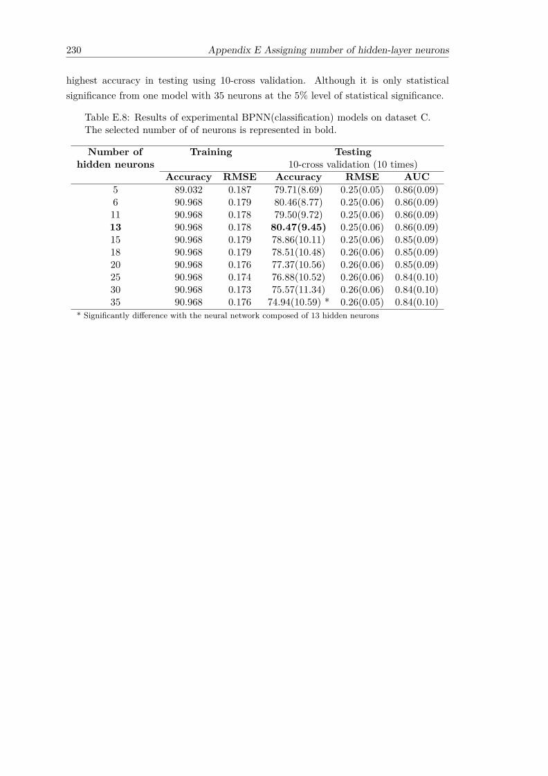
230 Appendix E Assigning number of hidden-layer neurons
highest accuracy in testing using 10-cross validation. Although it is only statisticalsignificance from one model with 35 neurons at the 5% level of statistical significance.
Table E.8: Results of experimental BPNN(classification) models on dataset C.The selected number of of neurons is represented in bold.
Number of Training Testinghidden neurons 10-cross validation (10 times)
Accuracy RMSE Accuracy RMSE AUC5 89.032 0.187 79.71(8.69) 0.25(0.05) 0.86(0.09)6 90.968 0.179 80.46(8.77) 0.25(0.06) 0.86(0.09)11 90.968 0.178 79.50(9.72) 0.25(0.06) 0.86(0.09)13 90.968 0.178 80.47(9.45) 0.25(0.06) 0.86(0.09)15 90.968 0.179 78.86(10.11) 0.25(0.06) 0.85(0.09)18 90.968 0.179 78.51(10.48) 0.26(0.06) 0.85(0.09)20 90.968 0.176 77.37(10.56) 0.26(0.06) 0.85(0.09)25 90.968 0.174 76.88(10.52) 0.26(0.06) 0.84(0.10)30 90.968 0.173 75.57(11.34) 0.26(0.06) 0.84(0.10)35 90.968 0.176 74.94(10.59) * 0.26(0.05) 0.84(0.10)
* Significantly difference with the neural network composed of 13 hidden neurons

Appendix F
Computational example ofimportance measures
F.1 Computational example for computing importance fromMultiple Linear Regression
This section illustrates the computational example for obtaining importance shown inthe third column of Table 5.9 from the regression coefficients shown in Figure F.1 andTable F.1.
The regression coefficients produced by SAS enterprise miner are unstandardized co-efficients however the standardized coefficients are preferable. Hence, these unstan-dardized coefficients were converted into standardized coefficients by multiplying eachunstandardized coefficient with the proportion of standard deviation of the attributeand standard deviation of Satisfaction (value = 1.035).
Importance of each attribute can be computed as percentage contribution of the stan-dardized coefficients in which a negative one is set as zero. The standardized coefficientsand importance are presented in the fourth and fifth column of Table F.1 respectively.
Table F.1: Unstandardized and standardized coefficients of MLR, and impor-tance of attribute in dataset A
Attribute Unstandardized Std. Standardized ImportanceCoefficients Deviation Coefficients
Equipment and System 0.1915 0.987 0.183 18.769Sales Support 0.0483 1.384 0.065 6.667Technical Support 0.362 1.137 0.398 40.821Supplies and Orders 0.1495 1.009 0.146 14.974Purchasing Support -0.00499 1.294 -0.006 0.000Contracts and Pricing 0.1687 1.12 0.183 18.769
231

232 Appendix F Computational example of importance measures
FigureF.1:
Result
ofmultiple
linearregression
implem
entedon
datasetA

Appendix F Computational example of importance measures 233
F.2 Computational example for computing importance fromOrdinal Linear Regression
This section illustrates the computational example for obtaining importance shown inthe fourth column of Table 5.9 from the regression coefficients shown in Figure F.2.
Before the importance are calculated from regression coefficients, the sign of regressioncoefficients obtained from SAS are reversed and shown in the first column of Table F.2.This is because SAS internally changes the sign of coefficients in estimating coefficientsdepending on the option ascending order or descending order. Importance of each at-tribute can be computed as percentage contribution of the standardized coefficients inwhich a negative one is set as zero, and presented in the second column of Table F.2.
Table F.2: Estimated coefficients of OLR and importance of attribute in datasetA
Attribute Estimated ImportanceCoefficients
Equipment and System 0.231 17.408Sales Support 0.073 5.501Technical Support 0.625 47.099Supplies and Orders 0.171 12.886Purchasing Support -0.046 0.000Contracts and Pricing 0.227 17.106
F.3 Computational example for computing importance fromneural network
This section illustrates the computational example for obtaining importance shown inthe fifth column of Table 5.9 from the connection weights of neural network shownin Table F.3 based on the procedure to compute attribute’s importance described inSection 3.3.3.
Given the connection weights of 6-2-1 neural network for dataset A as shown in TableF.3, the computation process for obtaining importance is as follows:
1. Input-Hidden layer computation. The proportion of each input-hidden connec-tion weights shown in TableF.5 are calculated by dividing each absolute weight by thesum of absolute weights for all inputs corresponding to each hidden layer displayed inTable F.4.e.g. P11= w11
SH1= 0.459
2.067 = 0.222

234 Appendix F Computational example of importance measures
FigureF.2:
Result
ofordinallinearregression
implem
entedon
datasetA

Appendix F Computational example of importance measures 235
Table F.3: neural weights of 6-2-1 network
Input/Hidden H1 H2Equipment and System -0.45945 -0.51086Sales Support -0.61236 0.081693Technical Support -0.09916 -0.97187Supplies and Orders -0.15282 -0.47836Purchasing Support 0.363219 -0.13334Contracts and Pricing -0.38013 -0.48767
Output/Hidden H1 H2Satisfaction -0.69225 -1.32191
Table F.4: Absolute value of input-hidden connection weights
Input/Hidden H1 H2Equipment and System w11 = 0.459 w12 = 0.511Sales Support w21 = 0.612 w22 = 0.082Technical Support w31 = 0.099 w32 = 0.972Supplies and Orders w41 = 0.153 w42 = 0.478Purchasing Support w51 = 0.363 w52 = 0.133Contracts and Pricing w61 = 0.380 w62 = 0.488Sum SH1 = 2.067 SH2 = 2.664
Table F.5: Proportion of input-hidden connection weights
Input/Hidden H1 H2Equipment and System P11 = 0.222 P12 = 0.192Sales Support P21 = 0.296 P22 = 0.031Technical Support P31 = 0.048 P32 = 0.365Supplies and Orders P41 = 0.074 P42 = 0.180Purchasing Support P51 = 0.176 P52 = 0.050Contracts and Pricing P61 = 0.184 P62 = 0.183Sum 1.000 1.000
2. Hidden-Output layer computation. The total hidden-output weights of eachhidden neurons are computed as the sum of the absolute value of all outputs correspond-ing to each hidden layer. Since, there is only one output neuron in this example, thetotal sum is equal to the the absolute value of hidden-output weights as shown in TableF.6.
Table F.6: Absolute value of hidden-output connection weights
Output/Hidden H1 H2Satisfaction w11 = 0.692 w12 = 1.322Sum SO1 = 0.692 SO2 = 1.322
3. Contribution of Input-Hidden weights and Hidden-Output weights. Thecontribution of each neuron to the output via each hidden neuron shown in Table F.7 is

236 Appendix F Computational example of importance measures
computed by multiplying the proportion of each input-hidden connection weight (TableF.5) by total output weight of the corresponding hidden neuron (Table F.6).e.g. C11= P11 × SO1 = 0.222 × 0.692 = 0.154
Table F.7: The contribution of each neuron to the output
Input/Hidden H1 H2Equipment and System C11= 0.154 C12 = 0.254Sales Support C21= 0.205 C22 = 0.041Technical Support C31 = 0.033 C32 = 0.482Supplies and Orders C41 = 0.051 C42 = 0.237Purchasing Support C51 =0.122 C52 = 0.066Contracts and Pricing C61 =0.127 C62 = 0.242
4. Relative importance computation. The relative importance shown in Table F.8 is calculated as the sum of the contribution of each neuron corresponding input layer(Table F.7) divided by overall contribution of all neurons in the network, and multipliedby 100.e.g. S1 = C11 + C12 = 0.154 + 0.254 = 0.407 andRI1 = S1
(S1+S2+...+S6)× 100 = 0.407
2.014 × 100 = 20.226
Table F.8: The relative importance of each attribute
Input Sum of contribution Relative Importance (%)Equipment and System S1 = 0.407 RI1 = 20.23Sales Support S2 = 0.246 RI2 = 12.19Technical Support S3 = 0.515 RI3 = 25.59Supplies and Orders S4 = 0.289 RI4 = 14.33Purchasing Support S5 = 0.188 RI5 = 9.32Contracts and Pricing S6 = 0.369 RI6 = 18.34Sum 2.014 100.000
F.4 Computational example for computing importance fromNaïve Bayes
This section illustrates the computational example for obtaining importance shown in theseventh column of Table 5.9 from the conditional probability distribution generated byNaïve Bayes. Regarding the model construction on dataset A, Naïve Bayes run by usingWEKA generated six conditional probability tables corresponded to each attribute.
For each conditional probability table, the importance of each attribute is calculatedbased on the procedure to compute attribute’s importance described in Step 2 of Sec-tion 3.3.4. The computational process is illustrated as follow:
1. Entropy of each attribute. The entropy of attribute h(Xi) is computed asEquation 3.7, where P (Xi = a) is the probability of each attribute with the satisfaction
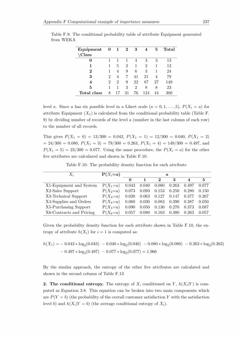
Appendix F Computational example of importance measures 237
Table F.9: The conditional probability table of attribute Equipment generatedfrom WEKA
Equipment 0 1 2 3 4 5 Total\Class
0 1 1 1 4 3 3 131 1 5 2 1 2 1 122 1 4 9 6 3 1 243 2 4 7 41 21 4 794 2 2 9 22 87 27 1495 1 1 3 2 8 8 23
Total class 8 17 31 76 124 44 300
level a. Since a has six possible level in a Likert scale (a = 0, 1, . . . , 5), P (Xi = a) forattribute Equipment (X1) is calculated from the conditional probability table (Table F.9) by dividing number of records of the level a (number in the last column of each row)to the number of all records.
This gives P (X1 = 0) = 13/300 = 0.043, P (X1 = 1) = 12/300 = 0.040, P (X1 = 2)
= 24/300 = 0.080, P (X1 = 3) = 79/300 = 0.263, P (X1 = 4) = 149/300 = 0.497, andP (X1 = 5) = 23/300 = 0.077. Using the same procedure, the P (Xi = a) for the otherfive attributes are calculated and shown in Table F.10.
Table F.10: The probability density function for each attribute
Xi P(Xi=a) a0 1 2 3 4 5
X1-Equipment and System P(X1=a) 0.043 0.040 0.080 0.263 0.497 0.077X2-Sales Support P(X2=a) 0.073 0.093 0.153 0.250 0.280 0.150X3-Technical Support P(X3=a) 0.020 0.063 0.127 0.147 0.377 0.267X4-Supplies and Orders P(X4=a) 0.060 0.030 0.083 0.390 0.387 0.050X5-Purchasing Support P(X5=a) 0.090 0.050 0.130 0.270 0.373 0.087X6-Contracts and Pricing P(X6=a) 0.057 0.080 0.163 0.380 0.263 0.057
Given the probability density function for each attribute shown in Table F.10, the en-tropy of attribute h(Xi) for i = 1 is computed as:
h(X1) =− 0.043 ∗ log2(0.043) − 0.040 ∗ log2(0.040) − 0.080 ∗ log2(0.080) − 0.263 ∗ log2(0.263)
− 0.497 ∗ log2(0.497) − 0.077 ∗ log2(0.077) = 1.966
By the similar approach, the entropy of the other five attributes are calculated andshown in the second column of Table F.13
2. The conditional entropy. The entropy of Xi conditioned on Y , h(Xi|Y ) is com-puted as Equation 3.8. This equation can be broken into two main components whichare P (Y = b) (the probability of the overall customer satisfaction Y with the satisfactionlevel b) and h(Xi|Y = b) (the average conditional entropy of Xi).

238 Appendix F Computational example of importance measures
P (Y = b) is a class distribution for the satisfaction level b (b = 0, 1, . . . , 5), calculatedfrom the conditional probability table (Table F.9) by dividing number of records of thelevel b (number in the last row of each column) to the number of all records. This givesP (Y = 0) = 8/300 = 0.027, P (Y = 1) = 17/300 = 0.057, P (Y = 2) = 31/300 = 0.103,P (Y = 3) = 76/300 = 0.253, P (Y = 4) = 124/300 = 0.413, and P (Y = 5) = 44/300 =0.147.
h(Xi|Y = b) can be computed from Equation 3.9, where P (Xi = a|Y = b) is thedistribution of Xi = a condition on Y = b. P (Xi = a|Y = b) is calculated from theconditional probability table by dividing number of records of the level a for attributeXi to the number of records of the level b for overall customer satisfaction Y .
For instance, given the conditional probability table of attribute “Equipment” as shownin Table F.9, the computational of P (X1 = a|Y = b) would be P (X1 = 0|Y = 0) = 1/8= 0.125, P (X1 = 1|Y = 0) = 1/8 = 0.125, . . . , P (X1 = 0|Y = 1) = 1/17 = 0.059,. . ., P (X1 = 5|Y = 5) = 8/44 = 0.182. In summary, there are 36 combinations in thiscomputation process since both a and b have six possible levels. The specific results ofP (X1 = a|Y = b) are provided in Table F.11.
Table F.11: Computational results of P (X1 = a|Y = b) (attribute Equipment)
ba 0 1 2 3 4 50 0.125 0.059 0.032 0.053 0.024 0.0681 0.125 0.294 0.065 0.013 0.016 0.0232 0.125 0.235 0.290 0.079 0.024 0.0233 0.250 0.235 0.226 0.539 0.169 0.0914 0.250 0.118 0.290 0.289 0.702 0.6145 0.125 0.059 0.097 0.026 0.065 0.182
Based on computational results of P (X1 = a|Y = b) shown in Table F.11, h(Xi|Y = b)
for i = 1 and b = 0 is computed as:
h(X1|Y = 0) =− 0.125 ∗ log2(0.125) − 0.125 ∗ log2(0.125) − 0.125 ∗ log2(0.125)
− 0.250 ∗ log2(0.250) − 0.250 ∗ log2(0.250) − 0.125 ∗ log2(0.125) = 2.500
By the similar approach, the entropy of h(X1|Y = b) for b = 1, . . . , 5 are computed andshown in Table F.12.
Table F.12: The average conditional entropy of attribute Equipment , h(X1|Y =b)
b0 1 2 3 4 5
h(X1|Y = b) 2.500 2.346 2.262 1.731 1.404 1.706
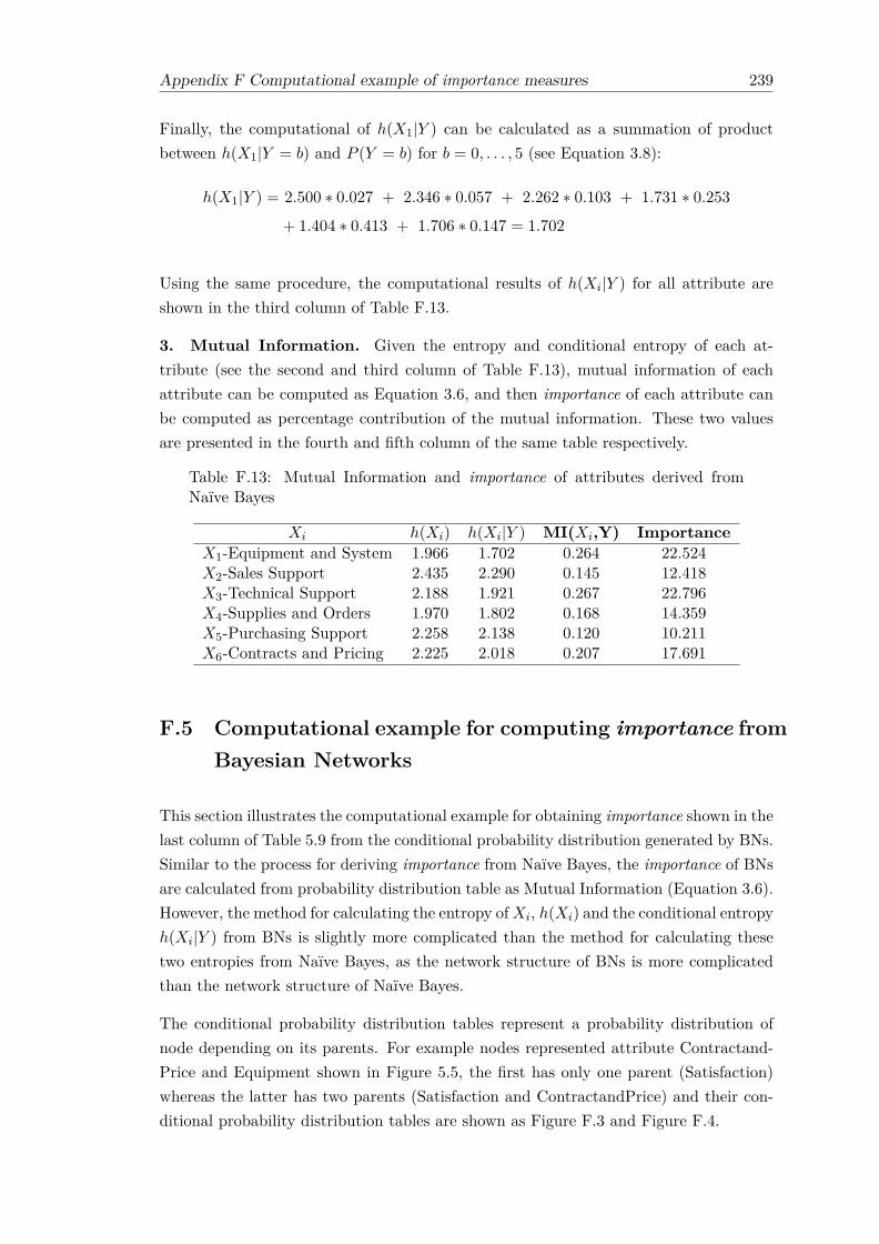
Appendix F Computational example of importance measures 239
Finally, the computational of h(X1|Y ) can be calculated as a summation of productbetween h(X1|Y = b) and P (Y = b) for b = 0, . . . , 5 (see Equation 3.8):
h(X1|Y ) = 2.500 ∗ 0.027 + 2.346 ∗ 0.057 + 2.262 ∗ 0.103 + 1.731 ∗ 0.253
+ 1.404 ∗ 0.413 + 1.706 ∗ 0.147 = 1.702
Using the same procedure, the computational results of h(Xi|Y ) for all attribute areshown in the third column of Table F.13.
3. Mutual Information. Given the entropy and conditional entropy of each at-tribute (see the second and third column of Table F.13), mutual information of eachattribute can be computed as Equation 3.6, and then importance of each attribute canbe computed as percentage contribution of the mutual information. These two valuesare presented in the fourth and fifth column of the same table respectively.
Table F.13: Mutual Information and importance of attributes derived fromNaïve Bayes
Xi h(Xi) h(Xi|Y ) MI(Xi,Y) ImportanceX1-Equipment and System 1.966 1.702 0.264 22.524X2-Sales Support 2.435 2.290 0.145 12.418X3-Technical Support 2.188 1.921 0.267 22.796X4-Supplies and Orders 1.970 1.802 0.168 14.359X5-Purchasing Support 2.258 2.138 0.120 10.211X6-Contracts and Pricing 2.225 2.018 0.207 17.691
F.5 Computational example for computing importance fromBayesian Networks
This section illustrates the computational example for obtaining importance shown in thelast column of Table 5.9 from the conditional probability distribution generated by BNs.Similar to the process for deriving importance from Naïve Bayes, the importance of BNsare calculated from probability distribution table as Mutual Information (Equation 3.6).However, the method for calculating the entropy ofXi, h(Xi) and the conditional entropyh(Xi|Y ) from BNs is slightly more complicated than the method for calculating thesetwo entropies from Naïve Bayes, as the network structure of BNs is more complicatedthan the network structure of Naïve Bayes.
The conditional probability distribution tables represent a probability distribution ofnode depending on its parents. For example nodes represented attribute Contractand-Price and Equipment shown in Figure 5.5, the first has only one parent (Satisfaction)whereas the latter has two parents (Satisfaction and ContractandPrice) and their con-ditional probability distribution tables are shown as Figure F.3 and Figure F.4.

240 Appendix F Computational example of importance measures
The table size of the conditional probability distribution of attribute ContractandPriceis 6 x 6 (see Figure F.3). Each cell indicates probability of ContractandPrice givenSatisfaction where value of ContractandPrice is equal to a and value of Satisfaction isequal to b.
Figure F.3: The conditional probability distribution of attribute Contractand-Price
The table size of the conditional probability distribution of Equipment is 36 x 6 (seeFigure F.4). Number of rows in the table is the combination of all possible valuesof two parent nodes of Equipment. Both Satisfaction and ContractandPrice have 6possible values 0-5 therefore their combination is 36. Each cell indicates probabilityof Equipment given Satisfaction and ContractandPrice where Equipment is equal to a,value of Satisfaction is equal to b and value of ContractandPrice is equal to c.
F.5.1 Pre-calculation procedure
There is one pre-calculation procedure to calculate the entropy of Xi, h(Xi) and theconditional entropy h(Xi|Y ) from BNs, which is the calculation of P (Xi = a) andP (Xi|Y = b). Regarding the two types of conditional probability distribution tables,method for calculating P (Xi = a) and P (Xi|Y = b), can be divided in two cases:attribute with one parent (e.g. attribute ContractandPrice) and attribute with twoparents (e.g. attribute Equipment).
1. Calculate P (Xi = a) and P (Xi|Y = b) on attribute Xi that has one parent
For the case of attribute with one parent, P (Xi|Y = b) can be directly obtained asthe conditional probability distribution table generated from WEKA. And then prob-ability distribution of each attribute P (Xi = a) can be computed based on the condi-tional probability distribution table by using the law of total probability1(also known asmarginalization).
1www.en.wikipedia.org/wiki/Law_of_total_probability
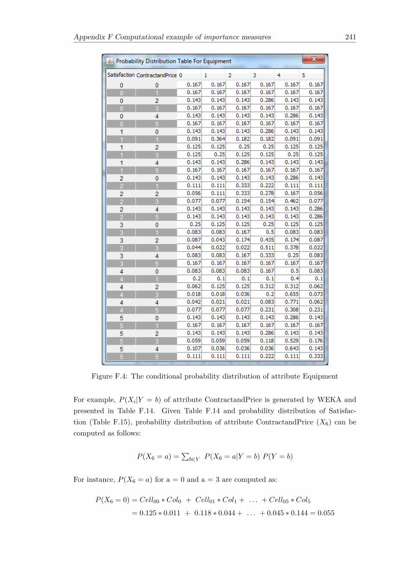
Appendix F Computational example of importance measures 241
Figure F.4: The conditional probability distribution of attribute Equipment
For example, P (Xi|Y = b) of attribute ContractandPrice is generated by WEKA andpresented in Table F.14. Given Table F.14 and probability distribution of Satisfac-tion (Table F.15), probability distribution of attribute ContractandPrice (X6) can becomputed as follows:
P (X6 = a) =∑
b∈Y P (X6 = a|Y = b) P (Y = b)
For instance, P (X6 = a) for a = 0 and a = 3 are computed as:
P (X6 = 0) = Cell00 ∗ Col0 + Cell01 ∗ Col1 + . . . + Cell05 ∗ Col5
= 0.125 ∗ 0.011 + 0.118 ∗ 0.044 + . . . + 0.045 ∗ 0.144 = 0.055

242 Appendix F Computational example of importance measures
Table F.14: The probability of attribute ContractandPrice conditioned on Sat-isfaction generated from WEKA
ContractandPrice (X6)\Satisfaction (Y) ba 0 1 2 3 4 50 0.125 0.118 0.065 0.039 0.056 0.0451 0.125 0.353 0.129 0.092 0.040 0.0232 0.250 0.176 0.419 0.237 0.089 0.0453 0.125 0.176 0.258 0.526 0.403 0.2734 0.250 0.118 0.065 0.092 0.347 0.5235 0.125 0.059 0.065 0.013 0.065 0.091
Table F.15: The probability distribution of Satisfaction generated from WEKA
0 1 2 3 4 5Satisfaction (Y) 0.011 0.044 0.096 0.263 0.441 0.144
P (X6 = 3) = Cell30 ∗ Col0 + Cell31 ∗ Col1 + . . . + Cell35 ∗ Col5
= 0.125 ∗ 0.011 + 0.176 ∗ 0.044 + . . . + 0.273 ∗ 0.144 = 0.390
This computation is processed for other attribute’s value which produced the table ofprobability distribution of attribute ContractandPrice shown in Table F.16.
Table F.16: The probability of attribute ContractandPrice
ContractandPrice (X6) Probability0 0.0551 0.0752 0.1593 0.3904 0.2675 0.055
2. Calculate P (Xi = a) and P (Xi|Y = b) on attribute Xi that has two parents
In case attribute Xi has two parents in which its conditional probability distributioncontains value in this form P (Xi|Y,Xj), P (Xi|Y = b) can be computed by using the lawof total probability as previously stated.
Considering attribute Equipment (X1) which has two parents namely Satisfaction andContractandPrice (X6), P (X1 = a|Y = b) can be calculated from P (X1 = a|Y = b,X6)
as follows, where a and b are the possible value of attribute and Satisfaction which are0-5.
P (X1 = a|Y = b) =∑
c∈X6P (X1 = a|Y = b,X6) P (X6)
Given the first six rows in which Satisfaction = 0 from 36 rows (Figure F.4) of theconditional probability distribution of attribute Equipment as shown in Table F.17 and

Appendix F Computational example of importance measures 243
probability distribution of attribute CondandPrice (X6), shown in Table F.16, condi-tional probability of attribute X1 = a given Y = b can be computed as the summationof product of value in Cellbca of Table F.17 and value in Rowc of Table F.16 where valuerange of c is 0-5.
Table F.17: Part of the probability distribution table of attribute Equipmentconditioned on two parents generated from WEKA
Parent Probability distribution of EquipmentSatisfaction ContractandPrice 0 1 2 3 4 5
(b) (c) (a)0 0.167 0.167 0.167 0.167 0.167 0.1671 0.167 0.167 0.167 0.167 0.167 0.167
0 2 0.143 0.143 0.143 0.286 0.143 0.1433 0.167 0.167 0.167 0.167 0.167 0.1674 0.143 0.143 0.143 0.143 0.286 0.1435 0.167 0.167 0.167 0.167 0.167 0.167
For instance, P (X1 = a|Y = b) for a = 0 and b = 0 is computed as:
P (X1 = 0|Y = 0) = Cell000 ∗Row0 + Cell010 ∗Row1 + . . . + Cell050 ∗Row5
= 0.167 ∗ 0.055 + 0.167 ∗ 0.075 + . . . + 0.167 ∗ 0.055
= 0.009 + 0.012 + . . . + 0.009 = 0.157
For instance, P (X1 = a|Y = b) for a = 3 and b = 0 is computed as:
P (X1 = 3|Y = 0) = Cell003 ∗Row0 + Cell013 ∗Row1 + Cell023 ∗Row2 + . . . + Cell053 ∗Row5
= 0.167 ∗ 0.055 + 0.167 ∗ 0.075 + 0.286 ∗ 0.159 + . . . + 0.167 ∗ 0.055
= 0.009 + 0.012 + 0.045 + . . . + 0.009 = 0.179
This computation is processed for all combination of ContractandPrice and Satisfactionwhich produced the table of conditional probability distribution of attribute Equipmentshown in Table F.18.
Table F.18: The conditional probability distribution table of attribute Equip-ment
Equipment (X1)\ Satisfaction 0 1 2 3 4 5
0 0.157 0.13 0.101 0.082 0.052 0.1011 0.157 0.2 0.11 0.06 0.049 0.0822 0.157 0.195 0.192 0.109 0.056 0.0823 0.179 0.165 0.175 0.417 0.179 0.1334 0.195 0.179 0.276 0.264 0.585 0.4355 0.157 0.13 0.147 0.067 0.08 0.168

244 Appendix F Computational example of importance measures
The probability distribution of attribute Equipment P (Xi = a) then can be computedfrom Table F.18 and Table F.15 regarding the procedure described in the Step 1 of thepre-calculation procedure.
For instance, P (X1 = a) for a = 0 and a = 3 are computed as:
P (X1 = 0) = Cell00 ∗ Col0 + Cell01 ∗ Col1 + . . . + Cell05 ∗ Col5
= 0.157 ∗ 0.011 + 0.130 ∗ 0.044 + . . . + 0.101 ∗ 0.144 = 0.076
P (X1 = 3) = Cell30 ∗ Col0 + Cell31 ∗ Col1 + . . . + Cell35 ∗ Col5
= 0.179 ∗ 0.011 + 0.165 ∗ 0.044 + . . . + 0.133 ∗ 0.144 = 0.234
This computation is processed for other attribute’s value which produced the table ofprobability distribution of attribute Equipment shown in Table F.19.
Table F.19: The probability of attribute Equipment
Equipment (X1) Probability0 0.0761 0.0702 0.0943 0.2344 0.4275 0.099
F.5.2 Calculate importance as Mutual Information
1. Calculate Entropy of each attribute h(Xi)
Given the probability density function for attribute Equipment and CondandPrice shownin Table F.19 and Table F.16 respectively, the entropy of attribute h(Xi) for i = 1 andi = 6 are computed following Equation 3.7 :
h(X1) =− 0.076 ∗ log2(0.076) − 0.070 ∗ log2(0.070) − 0.094 ∗ log2(0.094)
− 0.234 ∗ log2(0.234) − 0.427 ∗ log2(0.427) − 0.099 ∗ log2(0.099) = 2.218
h(X6) =− 0.055 ∗ log2(0.055) − 0.075 ∗ log2(0.075) − 0.159 ∗ log2(0.159)
− 0.390 ∗ log2(0.390) − 0.267 ∗ log2(0.267) − 0.055 ∗ log2(0.055) = 2.200
By the similar approach, the entropy of the other four attributes are calculated andshown in the second column of Table F.21

Appendix F Computational example of importance measures 245
2. Calculate conditional entropy h(Xi|Y )
The entropy of Xi conditioned on Y , h(Xi|Y ) is computed as Equation 3.8. This equa-tion can be broken into two main components which are P (Y = b) (the probability ofthe overall customer satisfaction Y with the satisfaction level b) and h(Xi|Y = b) (theaverage conditional entropy of Xi).
In the context of this computational example, P (Y = b) is presented in Table F.15and h(Xi|Y = b) can be computed from Equation 3.9. Given Table F.15 and Table F.18 represents conditional probability distribution table of attribute Equipment P (X1 =
a|Y = b), conditional entropy of attribute Equipment h(X1|Y = b) for b = 0 can becomputed as follows:
h(X1|Y = 0) =− 0.157 ∗ log2(0.157) − 0.157 ∗ log2(0.157) − 0.157 ∗ log2(0.157)
− 0.179 ∗ log2(0.179) − 0.195 ∗ log2(0.195) − 0.157 ∗ log2(0.157) = 2.579
By the similar approach, the entropy of h(X1|Y = b) for b = 1, . . . , 5 are computed andshown in Table F.20.
Table F.20: The average conditional entropy of attribute Equipment, h(X1|Y =b)
b0 1 2 3 4 5
h(X1|Y = b) 2.579 2.564 2.499 2.184 1.855 2.266
Finally, the computational of h(X1|Y ) can be calculated as a summation of productbetween h(X1|Y = b) and P (Y = b) for b = 0, . . . , 5 (see Equation 3.8):
h(X1|Y ) = 2.579 ∗ 0.011 + 2.564 ∗ 0.044 + 2.499 ∗ 0.096 + 2.184 ∗ 0.263
+ 1.855 ∗ 0.441 + 2.266 ∗ 0.144 = 2.102
Using the same procedure, the computational results of h(Xi|Y ) for all attribute areshown in the third column of Table F.21.
3. Calculate Mutual Information. Given the entropy and conditional entropy ofeach attribute (see the second and third column of Table F.21), mutual information ofeach attribute can be computed as Equation 3.6, and then importance of each attributecan be computed as percentage contribution of the mutual information. These twovalues are presented in the fourth and fifth column of the same table respectively.

246 Appendix F Computational example of importance measures
Table F.21: Mutual Information and importance of attributes derived fromBayesian Networks
Xi h(Xi) h(Xi|Y ) MI(Xi,Y) ImportanceX1-Equipment and System 2.218 2.102 0.115 20.409X2-Sales Support 2.466 2.445 0.020 3.582X3-Technical Support 2.374 2.259 0.115 20.401X4-Supplies and Orders 2.275 2.197 0.077 13.661X5-Purchasing Support 2.399 2.357 0.042 7.432X6-Contracts and Pricing 2.200 2.005 0.195 34.515
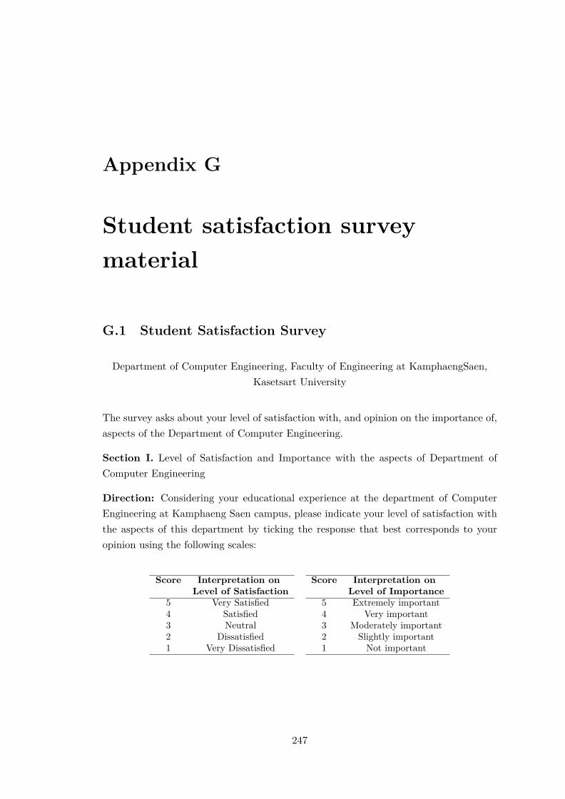
Appendix G
Student satisfaction surveymaterial
G.1 Student Satisfaction Survey
Department of Computer Engineering, Faculty of Engineering at KamphaengSaen,Kasetsart University
The survey asks about your level of satisfaction with, and opinion on the importance of,aspects of the Department of Computer Engineering.
Section I. Level of Satisfaction and Importance with the aspects of Department ofComputer Engineering
Direction: Considering your educational experience at the department of ComputerEngineering at Kamphaeng Saen campus, please indicate your level of satisfaction withthe aspects of this department by ticking the response that best corresponds to youropinion using the following scales:
Score Interpretation on Score Interpretation onLevel of Satisfaction Level of Importance
5 Very Satisfied 5 Extremely important4 Satisfied 4 Very important3 Neutral 3 Moderately important2 Dissatisfied 2 Slightly important1 Very Dissatisfied 1 Not important
247

248 Appendix G Student satisfaction survey material
1. Academic Personal Level of Satisfaction Level of Importance5 4 3 2 1 5 4 3 2 1
Teaching ability of teaching staffSubject expertise of teaching staffFriendliness of the teaching staffAvailability of teaching staffAdvice and support in learningOverall satisfaction level with Academic Personal
2. Teaching and Learning Level of Satisfaction Level of Importance5 4 3 2 1 5 4 3 2 1
Lecture materialse-learning resourcesAssessments (clarity and timely feedback)Class sizeAccurate and up-to-date unit contentTeaching facilities and classroom conditionOverall satisfaction level with Teaching andLearning
3. Administration Level of Satisfaction Level of Importance5 4 3 2 1 5 4 3 2 1
Knowledge of rules and procedures of staff mem-bersKnowledge of the information about courses, ex-ams, activities of staff membersInterest in solving the problems of student by staffmembersFriendliness of staff membersAbility of the staff members to provide servicesin a timely mannerOverall satisfaction level with Administration
4. Computer Facilities Level of Satisfaction Level of Importance5 4 3 2 1 5 4 3 2 1
Quality of computer facilities (Hardware andSoftware)Availability of computer facilitiesAvailability of internet accessAvailability of printing and photocopying facili-tiesOverall satisfaction level with Computer Facili-ties
5. Extra-Curricular Activities Level of Satisfaction Level of Importance5 4 3 2 1 5 4 3 2 1
Cultural exchange programs with foreign coun-triesField tripsMoral development activitiesHealth development activitiesInterpersonal skills development activitiesPersonal learning and thinking skills developmentactivitiesSocial volunteer activitiesOverall satisfaction level with Extra-CurricularActivities

Appendix G Student satisfaction survey material 249
6. Additional services Level of Satisfaction Level of Importance5 4 3 2 1 5 4 3 2 1
Financial aid for studentsMedical support to studentsDepartment website (Updated content andeasy to find information)LibraryOverall satisfaction level with Additional ser-vices
Section II. Personal InformationDirection: Please tick the circle that best corresponds to your answer for each questionbelow
1. Gender ◦ Male ◦ Female
2. Study Level ◦ 1 ◦ 2 ◦ 3 ◦ 4 ◦ other (specify)
3. Program ◦ Regular ◦ Special
Thank you for taking the time to complete this questionnaire

250 Appendix G Student satisfaction survey material
G.2 Participant Information sheet
Study Title: Mining Survey Data for SWOT analysisResearcher: Boonyarat PhadermrodEthics number: ERGO/FPSE/14268
Please read this information carefully before deciding to take part in this research. Ifyou are happy to participate you will be asked to sign a consent form.
What is the research about?I am completing a PhD research about mining survey data for SWOT analysiswhich aimed to generate prioritized SWOT factors based on the customer’s per-ception. To evaluate the proficiency of the proposed approach in the real-worldsituation, the case study of Department of Computer Engineering (DoCE), Kaset-sart University will be conducted. Through this case study, your response on thelevel of satisfaction and importance with the aspects of the DoCE will be analysedto produce SWOT using data mining technique.
Why have I been chosen?This research is trying to get a level of satisfaction with, and a level of the impor-tance of, aspects of the DoCE. Thus, you are chosen as you are a student in theDoCE, Kasetsart University (Bangkhen Campus and Kamphaeng Saen campus).
What will happen to me if I take part?The questionnaire will take no longer than 10 minutes to complete. There are threesections in the questionnaire. Section 1 and 2 asks about your level of satisfactionand importance with the aspects of the DoCE respectively. Section 3 asks aboutyour general information.
Are there any benefits in my taking part?By taking part, you have the opportunity to help us develop the new method togenerate SWOT based on satisfaction survey which can be used in government,academic institution and private company. You’re also help the DoCE to improvetheir quality of each aspect to meet your satisfaction.
Are there any risks involved?There is no risk involved for participants completing the questionnaire.
Will my participation be confidential?The name or student ID of the participants will not be taken and participationwill be kept anonymous. All data will be safe in a protected computer. All will bedestroyed once the research is completed.

Appendix G Student satisfaction survey material 251
What happens if I change my mind?You have the right to withdraw from doing the questionnaire at any time by exitingthe webpage.
What happens if something goes wrong?If you have any concern or complaint with this research please contacts me (Boon-yarat Phadermrod: [email protected]). If you have a trouble with the on-line forms, please contact the ECS School Office on [email protected] 02380592909.
Where can I get more information?If you would like more information on this research please feel free to contact me(Boonyarat Phadermrod: [email protected])
G.3 Result of language consistency translation test of stu-dent satisfaction survey
Remark: +1 the question/ instruction is consistent with the English version0 undecided about whether Thai question/ instruction is consistent with the
English version−1 the question/ instruction is not consistent with the English version
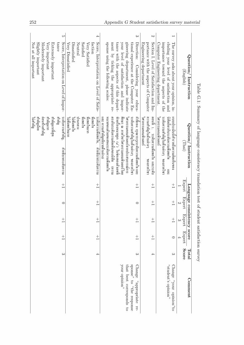
252 Appendix G Student satisfaction survey material
TableG.1:
Summary
oflanguageconsistency
translationtest
ofstudentsatisfaction
survey
Question/
InstructionQuestion/
InstructionLanguage
consistencyscore
TotalCom
ment
(English)(T
hai)Expert
ExpertExpert
ExpertScore
12
34
1Thesurvey
asksaboutyouropinion,in-cluding
yourlevel
ofsatisfaction
andim
portancetoward
theaspects
ofthe
Com
puterEngineering
department.
แบบประเมนนสารวจถงความคดเหนของนสตเกยวกบระดบความพงพอใจ
และระดบความสาคญในดานตางๆ
ของภาควชาวศวกรรมคอมพวเตอร
+1
+1
+1
03
Change
“youropinion”to
“student’sopinion”
2Section
I.LevelofSatisfactionand
Im-
portancewith
theaspects
ofCom
puterEngineering
department
ตอนท1.
ระดบความพงพอใจและระดบ
ความสาคญในดานตางๆของภาควชา
วศวกรรมคอมพวเตอร
+1
+1
+1
+1
4
3Direction:
Considering
youreduca-
tionalexperienceat
theCom
puterEn-
gineeringdepartm
ent,please
indicateyour
levelof
satisfactionand
impor-
tancewith
theaspects
ofthis
depart-ment
byticking
theappropriate
re-sponse
usingthe
following
scales:
คาชแจง:กรณาระบระดบความพงพอใจและระดบความสาคญในดานตางๆ
ของภาควชาวศวกรรมคอมพวเตอรจากประสบการณการศกษาณ
ภาควชาวศวกรรมคอมพวเตอรโดยทาเครองหมายถก
(X)ในชองของตวเลขท
ตรงกบระดบความคดเหนของนสต(ความ
หมายของตวเลขแสดงระดบความพงพอใจและความสาคญอธบายดานลาง)
+1
0+1
+1
3Change
“appropriatere-
sponse”to
“theresponse
thatbest
correspondsto
youropinion”
4Score,Interpretation
onLevelofSatis-
factionระดบความพงพอใจ,
คาอธบายระดบความพงพอใจ
+1
+1
+1
+1
4
VerySatisfied
พงพอใจมากSatisfied
พงพอใจNeutral
ปานกลางDissatisfied
ไมพงพอใจVery
Dissatisfied
ไมพงพอใจมาก5
Score,Interpretationon
LevelofImpor-
tanceระดบความสาคญ,
คาอธบายระดบความสาคญ
+1
0+1
+1
3
Extremely
important
สาคญมากทสดVery
important
สาคญมากModerately
important
คอนขางสาคญSlightly
important
สาคญนอยNot
atallim
portantไมสาคญ
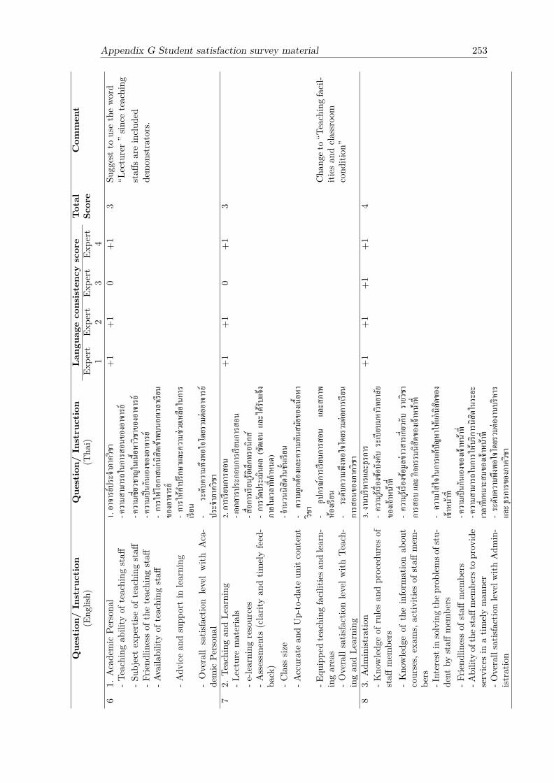
Appendix G Student satisfaction survey material 253
Que
stion/
Instruction
Que
stion/
Instruction
Lang
uage
consistenc
yscore
Total
Com
ment
(Eng
lish)
(Tha
i)Ex
pert
Expe
rtEx
pert
Expe
rtSc
ore
12
34
61.
Acade
mic
Person
al1.อาจาร
ยประจาภ
าควช
า+1
+1
0+1
3Su
ggestto
usethewo
rd-T
eachingab
ility
ofteaching
staff
-ความ
สามารถ
ในการส
อนขอ
งอาจา
รย“L
ecturer”sin
ceteaching
-Sub
ject
expe
rtise
ofteaching
staff
-ความ
เชยวช
าญใน
เนอหา
วชาของอาจาร
ยstaff
sareinclud
ed-F
riend
linessof
theteaching
staff
-ความ
เปนกน
เองขอ
งอาจา
รยde
mon
strators.
-Availa
bilityof
teaching
staff
-การใ
หโอก
าสแก
นสตเข
าพบน
อกเวล
าเรยน
ของอาจา
รย-A
dvicean
dsupp
ortin
learning
-การใ
หคาปรก
ษาแล
ะความ
ชวยเห
ลอใน
การ
เรยน
-Overall
satis
faction
levelwith
Aca-
demic
Person
al-
ระดบ
ความพง
พอใจโ
ดยรวมต
ออาจา
รยปร
ะจาภาควช
า7
2.Te
aching
andLe
arning
2.การเร
ยนการส
อน+1
+1
0+1
3-L
ecture
materials
-เอกส
ารประกอ
บการเ
รยนก
ารสอน
-e-le
arning
resources
-สอก
ารเรยนร
อเลกท
รอนก
ส-A
ssessm
ents
(clarit
yan
dtim
elyfeed
-ba
ck)
-การว
ดประเมน
ผล(ชด
เจนแล
ะไดร
บแจง
ภายใน
เวลาทกาหน
ด)-C
lass
size
-จาน
วนนส
ตในช
นเรยน
-Accuratean
dUp-to-dateun
itcontent
-คว
ามถก
ตองและ
ความทน
สมยข
องเนอ
หาวช
า-E
quippe
dteaching
facilitiesa
ndlearn-
ingareas
-อป
กรณก
ารเรยนก
ารสอน
และส
ภาพ
หองเร
ยนCha
nget
o“T
eachingfacil-
ities
andclassroo
m-O
verallsatis
factionlevelw
ithTe
ach-
ingan
dLe
arning
-ระดบ
ความพง
พอใจโ
ดยรวมต
อการเ
รยน
การส
อนขอ
งภาควช
าcond
ition
”
83.
Adm
inist
ratio
n3.งาน
บรหา
รและ
ธรการ
+1
+1
+1
+1
4-K
nowledg
eof
rulesan
dproced
ures
ofstaff
mem
bers
-ความ
รเรองขอ
บงคบ
ระเบย
บมหา
วทยาล
ยขอ
งเจาห
นาท
-Kno
wledg
eof
theinform
ationab
out
courses,
exam
s,activ
ities
ofstaff
mem
-be
rs
-ความ
รเรองขอ
มลขาวส
ารเกย
วกบ
รายวช
าการส
อบแล
ะกจก
รรมน
สตขอ
งเจาห
นาท
-Interestinsolvingthep
roblem
sofstu-
dent
bystaff
mem
bers
-คว
ามใส
ใจในก
ารแกป
ญหาให
แกนส
ตของ
เจาหน
าท-F
riend
linessof
staff
mem
bers
-ความ
เปนกน
เองขอ
งเจาห
นาท
-Abilityof
thes
taffmem
bers
toprov
ide
services
inatim
elyman
ner
-ความ
สามารถ
ในการให
บรการน
สตใน
ระยะ
เวลาทเหม
าะสมข
องเจา
หนาท
-Overallsatis
factionlevelw
ithAdm
in-
istratio
n-ร
ะดบค
วามพง
พอใจโ
ดยรวมต
องาน
บรหา
รแล
ะธรก
ารของภาคว
ชา

254 Appendix G Student satisfaction survey material
Question/
InstructionQuestion/
InstructionLanguage
consistencyscore
TotalCom
ment
(English)(T
hai)Expert
ExpertExpert
ExpertScore
12
34
94.
Com
puterFacilities
4.บรการคอมพวเตอร+1
+1
+1
+1
4-Quality
ofcom
puterfacilities
(Hard-
wareand
Software)-คณภาพของอปกรณคอมพวเตอร(ฮารดแวรและซอฟตแวร)
-Availabilityofcom
puterfacilities
-ความพรอมใหบรการของอปกรณคอมพว-
เตอร-Availability
ofInternetaccess
-ความพรอมใหบรการเชอมตออนเตอรเนต-Availability
ofprinting
andphoto-
copyingfacilities
-ความพรอมใหบรการของเครองพมพและ
เครองถายเอกสาร-Overall
satisfactionlevel
with
Com
-puter
Facilities-ระดบความพงพอใจโดยรวมตองานบรการ
คอมพวเตอร10
5.Extra-C
urricularActivities
5.กจกรรมเสรมหลกสตร+1
+1
+1
+1
4-C
ulturalExchangeprogram
swith
for-eign
-โครงการแลกเปลยนวฒนธรรมกบตาง
ประเทศ-Field
trips-ทศนะศกษาดงาน
-Moraldevelopm
entactivities
-กจกรรมพฒนาคณธรรม-H
ealthdevelopm
entactivities
-กจกรรมพฒนาสขภาพ-Interpersonal
skillsdevelopm
entac-
tivities-กจกรรมพฒนาความสมพนธระหวางบคคล
-Personallearning
andthinking
skillsdevelopm
entactivities
-กจกรรมพฒนาทกษะการคดและการเรยนร
-Socialvolunteeractivities
-กจกรรมเพอสงคม-Overallsatisfaction
levelwith
Extra-Curricular
Activities
-ระดบความพงพอใจโดยรวมตอกจกรรม
เสรมหลกสตรของภาควชา11
6.Additionalservices
6.บรการดานอนๆ+1
+1
+1
+1
4-Financialaid
forstudents
-ความชวยเหลอดานการเงนแกนสต-M
edicalsupportto
students-การรกษาพยาบาลสาหรบนสต
-Departm
entwebsite(Updated
contentand
easyto
findinform
ation)-
เวบไซตประจาภาควชา(เนอหาทนสมย
และสามารถคนหาขอมลไดงาย)-Library
-หองสมด-Overall
satisfactionlevel
with
Addi-
tionalservices-ระดบความพงพอใจโดยรวมตอบรการดานอนๆของภาควชา
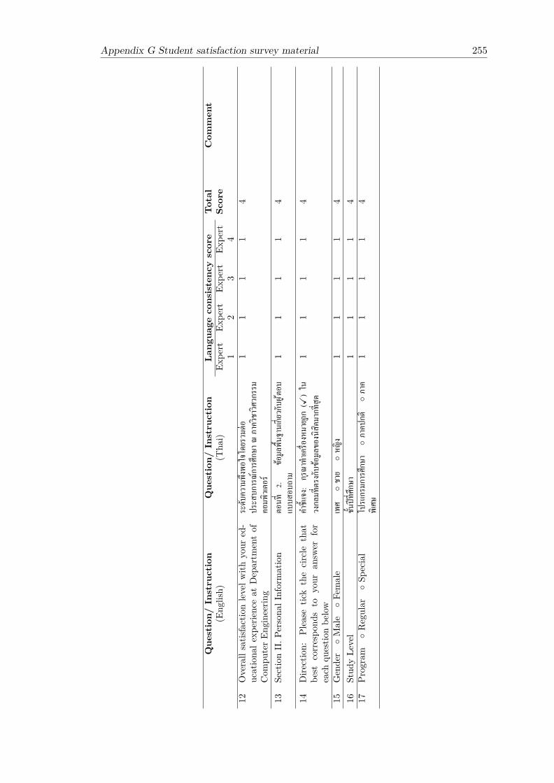
Appendix G Student satisfaction survey material 255
Que
stion/
Instruction
Que
stion/
Instruction
Lang
uage
consistenc
yscore
Total
Com
ment
(Eng
lish)
(Tha
i)Ex
pert
Expe
rtEx
pert
Expe
rtSc
ore
12
34
12Overallsatis
factionlevelw
ithyo
ured
-uc
ationa
lexp
erienc
eat
Dep
artm
entof
Com
puterEn
gine
ering
ระดบ
ความพง
พอใจโ
ดยรวมต
อปร
ะสบก
ารณการศกษ
าณภาคว
ชาวศ
วกรรม
คอมพ
วเตอร
11
11
4
13Se
ctionII.P
ersona
lInformation
ตอนท
2.ขอ
มลพน
ฐานเกย
วกบผ
ตอบ
แบบส
อบถาม
11
11
4
14Dire
ction:
Please
tick
thecircle
that
best
correspo
nds
toyo
uran
swer
for
each
questio
nbe
low
คาชแ
จง:กร
ณาทาเคร
องหม
ายถก
(X)ใ
นวงก
ลมทต
รงกบข
อมลข
องนส
ตมากทส
ด1
11
14
15Gen
der
◦Male
◦Fe
male
เพศ◦ชาย
◦หญ
ง1
11
14
16Stud
yLe
vel
ชนปท
ศกษา
11
11
417
Prog
ram
◦Regular
◦Sp
ecial
โปรแกร
มการศ
กษา
◦ภาคป
กต◦ภาค
พเศษ
11
11
4


Appendix H
Assumption checking of themultiple linear regressionon CPE-KU-KPS dataset
There were six attributes in CPE-KU-KPS dataset namely Academic Personal (Teacher),Teaching and Learning (Teaching), Administration (Admin), Computer Facilities (Comp-Fac), Extra-Curricular Activities (xActivity) and Additional Services (AddService). Tobuild regression model for each attribute, items related to the attribute were set as in-dependent variables and the overall student satisfaction (OCSstudent) was set as thedependent variable.
The assumptions of multiple linear regression were checked for each attribute in thedataset to ensure that the result of regression was valid. Assumption testing resultsfor each group of attribute are summarized in Table H.1 and explained in the followingsections.
Table H.1: Summary of assumption checking of MLR on six attributes of CPE-KU-KPS dataset
Assumptions AttributeTeacher Teaching Admin CompFac xActivity AddService
Normality of residual X X X X X XLinearity X X X X X XHomoscedasticity of residual X X X X X XIndependence of residual X X X X X XMulticollinearity X X X X X X
With regard to Table H.1, a symbol X indicates that the assumption was met and asymbol × indicates that the assumption was violated. According to the table it showsthat all assumptions were met across six attributes of the dataset.
257

258Appendix H Assumption checking of the multiple linear regression
on CPE-KU-KPS dataset
H.1 Normally distributed residual
For each group of attribute, assumption of normality was visually tested by observingthe histogram and normal P-P plot of the standardized residual. This assumption wasalso tested by observing the skewness and kurtosis of unstandardized residual in whichskew and kurtosis values between −1.0 and +1.0 are reasonable range to accept thatdata is reasonably close to normal (George and Mallery, 2003). Histograms and normalP-P plots of the standardized residual for each group were shown in Figure H.1 - H.6. And descriptive statistic of unstandardized residual for each group was shown inTable H.2.
(a) Histogram plot of residual (b) Normality plot of residual
Figure H.1: Histogram and normality plots of residual (Teacher)
(a) Histogram plot of residual (b) Normality plot of residual
Figure H.2: Histogram and normality plots of residual (Teaching)
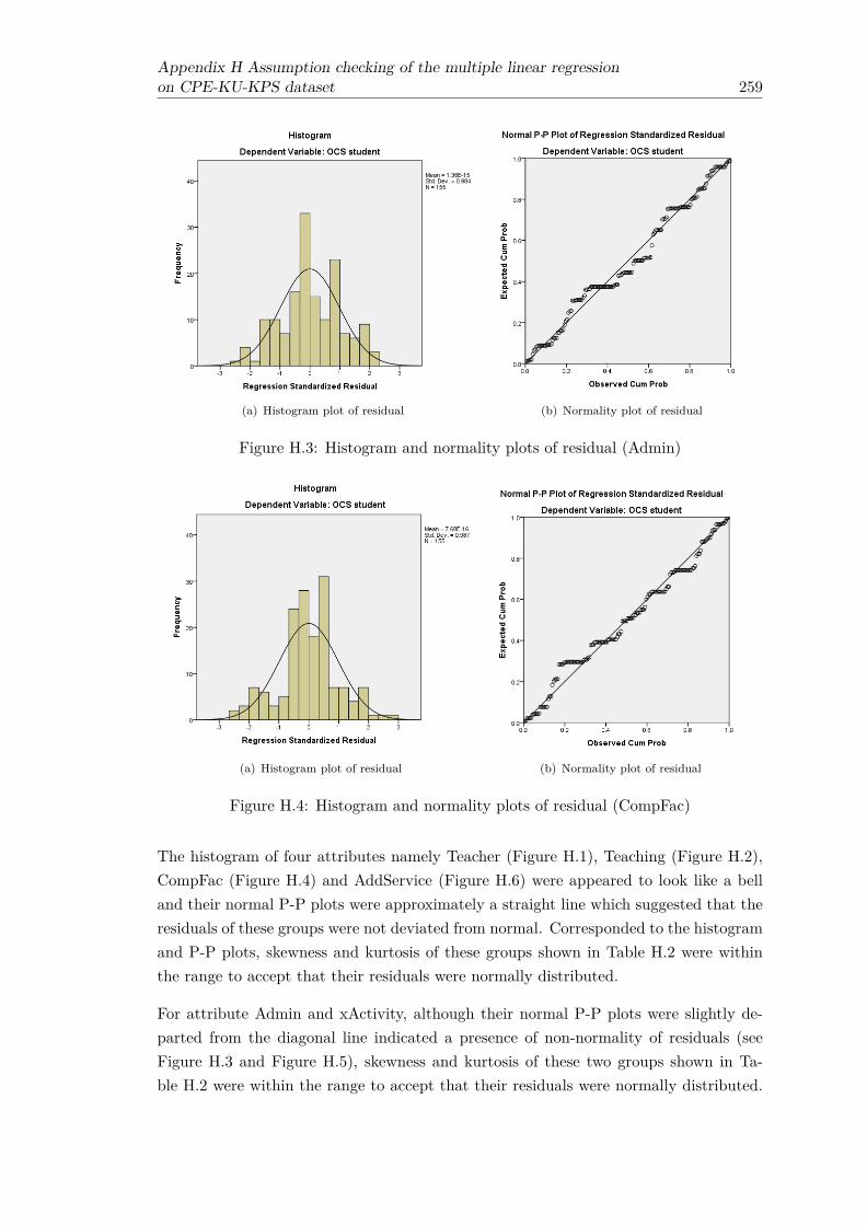
Appendix H Assumption checking of the multiple linear regressionon CPE-KU-KPS dataset 259
(a) Histogram plot of residual (b) Normality plot of residual
Figure H.3: Histogram and normality plots of residual (Admin)
(a) Histogram plot of residual (b) Normality plot of residual
Figure H.4: Histogram and normality plots of residual (CompFac)
The histogram of four attributes namely Teacher (Figure H.1), Teaching (Figure H.2),CompFac (Figure H.4) and AddService (Figure H.6) were appeared to look like a belland their normal P-P plots were approximately a straight line which suggested that theresiduals of these groups were not deviated from normal. Corresponded to the histogramand P-P plots, skewness and kurtosis of these groups shown in Table H.2 were withinthe range to accept that their residuals were normally distributed.
For attribute Admin and xActivity, although their normal P-P plots were slightly de-parted from the diagonal line indicated a presence of non-normality of residuals (seeFigure H.3 and Figure H.5), skewness and kurtosis of these two groups shown in Ta-ble H.2 were within the range to accept that their residuals were normally distributed.

260Appendix H Assumption checking of the multiple linear regression
on CPE-KU-KPS dataset
(a) Histogram plot of residual (b) Normality plot of residual
Figure H.5: Histogram and normality plots of residual (xActivity)
(a) Histogram plot of residual (b) Normality plot of residual
Figure H.6: Histogram and normality plots of residual (AddService)
Thus, it was reasonable to conclude that the residuals of all groups in the dataset werenormally distributed.
H.2 Linear relationship between independent and depen-dent variables
To check linearity assumption, a scatterplot of the standardized residual and standard-ized predicted value was drawn for each group of variables (see Figure H.7- H.12). Theresidual plot for predicted values of an outcome variable (OCS student) against theresiduals of all attributes showed that the dots were not constantly spread over the

Appendix H Assumption checking of the multiple linear regressionon CPE-KU-KPS dataset 261
Table H.2: Descriptive statistic of unstandardized residual for each attribute ofCPE-KU-KPS dataset
Unstandardized N Mean Std. Skewness KurtosisResidual Deviation Statistic Std. Error Statistic Std. Error
Teacher 155 0.00 0.4691 -0.435 0.195 -0.009 0.387Teaching 155 0.00 0.4445 0.227 0.195 0.204 0.387Admin 155 0.00 0.4809 0.048 0.195 -0.311 0.387CompFac 155 0.00 0.474 -0.006 0.195 0.262 0.387xActivity 155 0.00 0.4219 0.135 0.195 0.159 0.387AddService 155 0.00 0.4397 0.004 0.195 -0.476 0.387
horizontal line; however, there was no sign of any curve pattern. Therefore, it cannotconclude that the linearity assumption was violated.
Figure H.7: Scatterplot of residual for the relationship between five independentvariables of attribute Teacher and the OCS student
For each group of attribute, non-linear relationships can also be detected by addingcurve components which are quadratic (variable2) and cubic (variable3) to the regressionequation to see whether this increases the explained variance (R-square). Specifically,for each independent variable of each group, the R-square of the linear component andthe two curve components was statistically compared through the test of equality forseveral independent correlation coefficients (r) following an approach described in Kenny(1987). If there is no departure from linearity in the relationship, it is expected to seethat the difference between the linear correlation coefficient (r) and the non-linear (curve)correlation coefficient is not significantly different (p-value > 0.05).
Table H.3 shows the R-square of linear/non-linear components of each independentvariable of attribute Teacher against the OCS student. Regarding this table, R-squares

262Appendix H Assumption checking of the multiple linear regression
on CPE-KU-KPS dataset
Figure H.8: Scatterplot of residual for the relationship between six independentvariables of attribute Teaching and the OCS student
of the curve component of all variables of attribute Teacher were equal to or slightlyhigher than R-square of the linear component.
The test for equality of several independent correlation coefficients shown in Table H.4 indicated that there was no significant difference among correlations of the linear/non-linear components for each independent variable of attribute Teacher. Therefore, itwas reasonable to conclude that the relationship between each independent variable ofattribute Teacher and the OCS student is linear.
Table H.3: R-square of the components of regression equation (attributeTeacher)
Independent variable R-SquareLinear Quadratic Cubic
Teacher 1 0.260 0.261 0.261Teacher 2 0.269 0.270 0.270Teacher 3 0.189 0.189 0.189Teacher 4 0.186 0.186 0.186Teacher 5 0.207 0.209 0.209
Table H.5 shows the R-square of linear/non-linear components of each independentvariable of attribute Teaching against the OCS student. Regarding this table, R-squaresof the curve component of two variables named Teaching 1 and Teaching 6 were equalto or slightly higher than R-square of the linear component. R-squares of the curvecomponent of the other four variables named Teaching 2-5 were greatly higher thanR-squares of the linear component indicated a sign of non-linearity.

Appendix H Assumption checking of the multiple linear regressionon CPE-KU-KPS dataset 263
Figure H.9: Scatterplot of residual for the relationship between five independentvariables of attribute Admin and the OCS student
Table H.4: Chi-square statistic for the difference test of equality of correlations(attribute Teacher)
Independent variable χ2 df p-value EqualityTeacher 1 0.000 2 1.000 YesTeacher 2 0.000 2 1.000 YesTeacher 3 0.000 2 1.000 YesTeacher 4 0.000 2 1.000 YesTeacher 5 0.001 2 1.000 Yes
However, considering the test for equality of several independent correlation coefficientsreported in Table H.6, it showed that there was no significant difference among corre-lations of the linear/non-linear component for each independent variable of attributeTeaching. Therefore, it was reasonable to conclude that the relationship between eachindependent variable of attribute Teaching and the OCS student is linear.
Table H.5: R-square of the components of regression equation (attribute Teach-ing)
Independent variable R-SquareLinear Quadratic Cubic
Teaching 1 0.306 0.309 0.309Teaching 2 0.256 0.283 0.288Teaching 3 0.248 0.268 0.265Teaching 4 0.188 0.197 0.198Teaching 5 0.142 0.24 0.241Teaching 6 0.341 0.345 0.346

264Appendix H Assumption checking of the multiple linear regression
on CPE-KU-KPS dataset
Figure H.10: Scatterplot of residual for the relationship between four indepen-dent variables of attribute CompFac and the OCS student
Table H.6: Chi-square statistic for the difference test of equality of correlations(attribute Teaching)
Independent variable χ2 df p-value EqualityTeaching 1 0.002 2 0.999 YesTeaching 2 0.156 2 0.925 YesTeaching 3 0.062 2 0.969 YesTeaching 4 0.018 2 0.991 YesTeaching 5 1.993 2 0.369 YesTeaching 6 0.004 2 0.998 Yes
Table H.7 shows the R-square of linear/non-linear components of each independentvariable of attribute Admin against the OCS student. Regarding this table, R-squaresof the curve component of most variables were equal to or slightly higher than R-squareof the linear component. Only the variable named Admin 3 which its R-squares of thecurve component were greatly higher than its R-squares of the linear component.
Given R-square from Table H.7, the test for equality of several independent correlationcoefficients was conducted and the result was reported in Table H.8. The Table H.8showed that there was no significant difference among correlations of the linear/non-linear component for each independent variable of attribute Admin. Therefore, it wasreasonable to conclude that the relationship between each independent variable of at-tribute Admin and the OCS student is linear.
Table H.9 shows the R-square of linear/non-linear components of each independentvariable of attribute CompFac against the OCS student. Regarding this table, R-squares
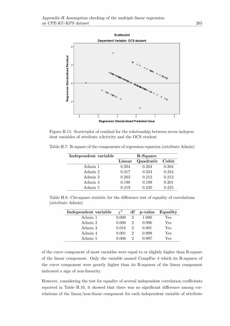
Appendix H Assumption checking of the multiple linear regressionon CPE-KU-KPS dataset 265
Figure H.11: Scatterplot of residual for the relationship between seven indepen-dent variables of attribute xActivity and the OCS student
Table H.7: R-square of the components of regression equation (attribute Admin)
Independent variable R-SquareLinear Quadratic Cubic
Admin 1 0.204 0.204 0.204Admin 2 0.317 0.324 0.324Admin 3 0.203 0.212 0.213Admin 4 0.198 0.199 0.201Admin 5 0.219 0.220 0.225
Table H.8: Chi-square statistic for the difference test of equality of correlations(attribute Admin)
Independent variable χ2 df p-value EqualityAdmin 1 0.000 2 1.000 YesAdmin 2 0.008 2 0.996 YesAdmin 3 0.018 2 0.991 YesAdmin 4 0.001 2 0.999 YesAdmin 5 0.006 2 0.997 Yes
of the curve component of most variables were equal to or slightly higher than R-squareof the linear component. Only the variable named CompFac 4 which its R-squares ofthe curve component were greatly higher than its R-squares of the linear componentindicated a sign of non-linearity.
However, considering the test for equality of several independent correlation coefficientsreported in Table H.10, it showed that there was no significant difference among cor-relations of the linear/non-linear component for each independent variable of attribute

266Appendix H Assumption checking of the multiple linear regression
on CPE-KU-KPS dataset
Figure H.12: Scatterplot of residual for the relationship between four indepen-dent variables of attribute AddService and the OCS student
CompFac. Therefore, it was reasonable to conclude that the relationship between eachindependent variable of attribute CompFac and the OCS student is linear.
Table H.9: R-square of the components of regression equation (attribute Comp-Fac)
Independent variable R-SquareLinear Quadratic Cubic
CompFac 1 0.296 0.300 0.308CompFac 2 0.317 0.322 0.324CompFac 3 0.165 0.165 0.165CompFac 4 0.278 0.281 0.294
Table H.10: Chi-square statistic for the difference test of equality of correlations(attribute CompFac)
Independent variable χ2 df p-value EqualityCompFac 1 0.019 2 0.990 YesCompFac 2 0.007 2 0.997 YesCompFac 3 0.000 2 1.000 YesCompFac 4 0.038 2 0.981 Yes
Table H.11 shows the R-square of linear/non-linear components of each independentvariable of attribute xActivity against the OCS student. Regarding this table, R-squaresof the curve component of most variables were equal to or slightly higher than R-squareof the linear component. Only the variables named xActivity 4 and xActivity 7 which
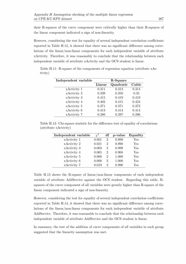
Appendix H Assumption checking of the multiple linear regressionon CPE-KU-KPS dataset 267
their R-squares of the curve component were critically higher than their R-squares ofthe linear component indicated a sign of non-linearity.
However, considering the test for equality of several independent correlation coefficientsreported in Table H.12, it showed that there was no significant difference among corre-lations of the linear/non-linear components for each independent variable of attributexActivity. Therefore, it was reasonably to conclude that the relationship between eachindependent variable of attribute xActivity and the OCS student is linear.
Table H.11: R-square of the components of regression equation (attribute xAc-tivity)
Independent variable R-SquareLinear Quadratic Cubic
xActivity 1 0.311 0.313 0.314xActivity 2 0.339 0.350 0.35xActivity 3 0.415 0.419 0.419xActivity 4 0.402 0.415 0.424xActivity 5 0.371 0.371 0.372xActivity 6 0.413 0.414 0.414xActivity 7 0.286 0.297 0.296
Table H.12: Chi-square statistic for the difference test of equality of correlations(attribute xActivity)
Independent variable χ2 df p-value EqualityxActivity 1 0.001 2 0.999 YesxActivity 2 0.021 2 0.990 YesxActivity 3 0.003 2 0.999 YesxActivity 4 0.065 2 0.968 YesxActivity 5 0.000 2 1.000 YesxActivity 6 0.000 2 1.000 YesxActivity 7 0.019 2 0.990 Yes
Table H.13 shows the R-square of linear/non-linear components of each independentvariable of attribute AddService against the OCS student. Regarding this table, R-squares of the curve component of all variables were greatly higher than R-square of thelinear component indicated a sign of non-linearity.
However, considering the test for equality of several independent correlation coefficientsreported in Table H.14, it showed that there was no significant difference among corre-lations of the linear/non-linear components for each independent variable of attributeAddService. Therefore, it was reasonable to conclude that the relationship between eachindependent variable of attribute AddService and the OCS student is linear.
In summary, the test of the addition of curve components of all variables in each groupsuggested that the linearity assumption was met.

268Appendix H Assumption checking of the multiple linear regression
on CPE-KU-KPS dataset
Table H.13: R-square of the components of regression equation (attributeAddService)
Independent variable R-SquareLinear Quadratic Cubic
AddService 1 0.236 0.250 0.260AddService 2 0.334 0.345 0.347AddService 3 0.257 0.264 0.282AddService 4 0.378 0.394 0.410
Table H.14: Chi-square statistic for the difference test of equality of correlations(attribute AddService)
Independent variable χ2 df p-value EqualityAddService 1 0.079 2 0.961 YesAddService 2 0.025 2 0.988 YesAddService 3 0.088 2 0.957 YesAddService 4 0.135 2 0.935 Yes
H.3 Homoscedasticity of residuals
The assumption is that the residuals at each level of the dependent variables had thesame variance. There are graphical and non-graphical methods for checking homoscedas-ticity. For the graphical method, the scatterplot of the standardized residual and stan-dardized predicted value for each attribute (Figure H.7- H.12) were reobserved. Althoughthe dots were not constantly spread over the horizontal line, a funnel shaped patterndid not appear. It may be inferred that this assumption was met.
For a non-graphical method, the Breusch-Pagan test for all group of attributes wasconducted. The null hypothesis of Breusch-Pagan test is homoscedasticity. If p-value ofthe test less than 0.05, it is suggested that the null hypothesis is rejected.
Table H.15: Breusch-Pagan test for the homoscedasticity of all groups
Group of Variables BP df p-value HomoscedasticityTeacher 2.328 1 0.127 YesTeaching 1.285 1 0.257 YesAdmin 0.745 1 0.388 Yes
CompFac 0.080 1 0.777 YesxActivity 0.974 1 0.324 YesAddService 0.333 1 0.564 Yes
Consistent with the graphical method, a non-graphical method using Breusch-Pagantest for all group presented in Table H.15 is suggested that the variance of the residualsis homogenous. Thereby the assumption was met.
Note that steps for conducting Breusch-Pagan test using SPSS is referred to Pryce (2002)and the validity of this test is depended on the normality of residual. The z-score of
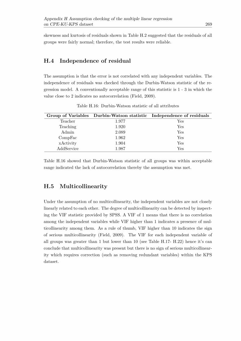
Appendix H Assumption checking of the multiple linear regressionon CPE-KU-KPS dataset 269
skewness and kurtosis of residuals shown in Table H.2 suggested that the residuals of allgroups were fairly normal; therefore, the test results were reliable.
H.4 Independence of residual
The assumption is that the error is not correlated with any independent variables. Theindependence of residuals was checked through the Durbin-Watson statistic of the re-gression model. A conventionally acceptable range of this statistic is 1 - 3 in which thevalue close to 2 indicates no autocorrelation (Field, 2009).
Table H.16: Durbin-Watson statistic of all attributes
Group of Variables Durbin-Watson statistic Independence of residualsTeacher 1.977 YesTeaching 1.920 YesAdmin 2.089 Yes
CompFac 1.962 YesxActivity 1.904 YesAddService 1.987 Yes
Table H.16 showed that Durbin-Watson statistic of all groups was within acceptablerange indicated the lack of autocorrelation thereby the assumption was met.
H.5 Multicollinearity
Under the assumption of no multicollinearity, the independent variables are not closelylinearly related to each other. The degree of multicollinearity can be detected by inspect-ing the VIF statistic provided by SPSS. A VIF of 1 means that there is no correlationamong the independent variables while VIF higher than 1 indicates a presence of mul-ticollinearity among them. As a rule of thumb, VIF higher than 10 indicates the signof serious multicollinearity (Field, 2009). The VIF for each independent variable ofall groups was greater than 1 but lower than 10 (see Table H.17- H.22) hence it’s canconclude that multicollinearity was present but there is no sign of serious multicollinear-ity which requires correction (such as removing redundant variables) within the KPSdataset.

270Appendix H Assumption checking of the multiple linear regression
on CPE-KU-KPS dataset
Table H.17: Collinearity Statistics (VIF) of five independent variables of at-tribute Teacher
Independent variable Collinearity Statistics (VIF)Teacher 1 1.890Teacher 2 1.930Teacher 3 1.578Teacher 4 1.929Teacher 5 2.073
Table H.18: Collinearity Statistics (VIF) of six independent variables of at-tribute Teaching
Independent variable Collinearity Statistics (VIF)Teaching 1 1.795Teaching 2 1.826Teaching 3 2.303Teaching 4 2.011Teaching 5 1.774Teaching 6 2.305
Table H.19: Collinearity Statistics (VIF) of five independent variables of at-tribute Admin
Independent variable Collinearity Statistics (VIF)Admin 1 2.821Admin 2 3.194Admin 3 3.000Admin 4 2.306Admin 5 2.918
Table H.20: Collinearity Statistics (VIF) of four independent variables of at-tribute CompFac
Independent variable Collinearity Statistics (VIF)CompFac 1 3.074CompFac 2 3.238CompFac 3 1.935CompFac 4 2.241
Table H.21: Collinearity Statistics (VIF) of seven independent variables of at-tribute xActivity
Independent variable Collinearity Statistics (VIF)xActivity 1 2.963xActivity 2 3.237xActivity 3 5.446xActivity 4 4.157xActivity 5 3.895xActivity 6 3.068xActivity 7 2.505
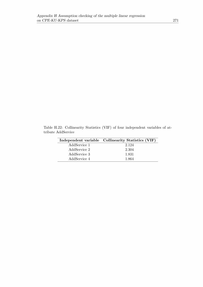
Appendix H Assumption checking of the multiple linear regressionon CPE-KU-KPS dataset 271
Table H.22: Collinearity Statistics (VIF) of four independent variables of at-tribute AddService
Independent variable Collinearity Statistics (VIF)AddService 1 2.124AddService 2 2.304AddService 3 1.831AddService 4 1.864


Appendix I
Assumption checking of themultiple linear regressionon CPE-KU-BKN dataset
There were six attributes in CPE-KU-BKN dataset namely Academic Personal (Teacher),Teaching and Learning (Teaching), Administration (Admin), Computer Facilities (Comp-Fac), Extra-Curricular Activities (xActivity) and Additional Services (AddService). Tobuild regression model for each attribute, items related to the attribute were set as in-dependent variables and the overall student satisfaction (OCSstudent) was set as thedependent variable.
The assumptions of multiple linear regression were checked for each attribute in thedataset to ensure that the result of regression was valid. Assumption testing resultfor each group of attribute are summarized in Table I.1 and explained in the followingsections.
Table I.1: Summary of assumption checking of MLR on six attributes of CPE-KU-BKN dataset
Assumptions AttributeTeacher Teaching Admin CompFac xActivity AddService
Normality of residual X X × X X XLinearity X X X X X XHomoscedasticity of residual X X X X X XIndependence of residual X X X X X XMulticollinearity X X X X X X
With regard to Table I.1, a symbol X indicates that the assumption was met and asymbol × indicates that the assumption was violated. According to the table it showsthat most assumptions were met across six attributes of the dataset except assumptionof normality for attribute Admin. Further steps were not performed to correct the
273

274Appendix I Assumption checking of the multiple linear regression
on CPE-KU-BKN dataset
assumption of normality of residual because the regression is fairly robust to violate ofnormality assumption. Beside violation of this assumption does not affect the regressioncoefficients which were the main focus of this study, the violation is only affected thesignificance tests for regression coefficients (Keith, 2014).
I.1 Normally distributed residual
For each group of attribute, the assumption of normality was visually tested by observingthe histogram and normal P-P plot of the standardized residual. This assumption wasalso tested by observing the skewness and kurtosis of unstandardized residual in whichskew and kurtosis values between −1.0 and +1.0 are reasonable ranges to accept thatdata is reasonably close to normal (George and Mallery, 2003).
Since the dataset was rather small, the significance tests of skewness and kurtosis werealso conducted by comparing the z-score of skewness and kurtosis against the value ofz-score at the significant level. Regarding to Tabachnick et al. (2001), the conventionalsignificant level of 0.001 was used to evaluate the significance of skewness and kurtosiswith small to moderate samples and the z-score associated to this conventional significantlevel is 3.29. Thus, the absolute value of z-score that greater than 3.29 indicated thatvalue of skewness and kurtosis is significantly different from zero which mean distributionis deviated from normal.
Histograms and normal P-P plots of the standardized residual for each group of attributeare shown in Figure I.1 - I.6. And descriptive statistic of unstandardized residual foreach group is shown in Table I.2. The histogram of group Teacher (Figure I.1), Admin(Figure I.3), CompFac (Figure I.4) and xActivity (Figure I.5) appeared to be asymmet-rical and their corresponding P-P plots were slightly deviated from the diagonal linewhich indicated that the distribution of residuals were not normal. In contrast, the his-togram of the other two groups named Teaching (Figure I.2) and AddService (Figure I.6) appeared to look like a bell and their normal P-P plots were approximately a straightline which suggested that the residuals of these variables were not deviated from normal.
Table I.2: Descriptive statistic of unstandardized residual for each attribute ofCPE-KU-BKN dataset
Unstandardized N Mean Std. Skewness KurtosisResidual Deviation Statistic Std.
Errorz-score Statistic Std.
Errorz-score
Teacher 43 0.000 0.557 -0.901 0.361 2.496 1.262 0.709 1.780Teaching 43 0.000 0.456 0.274 0.361 0.759 0.181 0.709 0.255Admin 43 0.000 0.619 -0.971 0.361 2.690 2.879 0.709 4.061CompFac 43 0.000 0.629 -0.861 0.361 2.385 2.104 0.709 2.968xActivity 43 0.000 0.396 0.483 0.361 1.338 -0.475 0.709 0.670AddService 43 0.000 0.513 0.031 0.361 0.086 0.348 0.709 0.491

Appendix I Assumption checking of the multiple linear regressionon CPE-KU-BKN dataset 275
(a) Histogram plot of residual (b) Normality plot of residual
Figure I.1: Histogram and normality plots of residual (Teacher)
(a) Histogram plot of residual (b) Normality plot of residual
Figure I.2: Histogram and normality plots of residual (Teaching)
Regarding to Table I.2, skew and kurtosis of Teaching, xActivity and AddService werewithin the range to accept that their residuals were normally distributed. On the otherhand, the kurtosis of Teacher, Admin and CompFac were greater than 1.0 indicatedthat the residuals were deviated from normal which corresponded to the histogram andP-P plots. Although the kurtosis of Teacher and CompFac were higher than 1.0, theirz-scores were less than 3.29. Thus, it was reasonable to conclude that the residuals ofthese two groups were normally distributed.
Table I.2 also showed that kurtosis z-score of Admin was higher than 3.29 indicated thatthe residual of this group was not normally distributed. Even though the assumption ofnormality of residual was not met for Admin group, further steps were not performed

276Appendix I Assumption checking of the multiple linear regression
on CPE-KU-BKN dataset
(a) Histogram plot of residual (b) Normality plot of residual
Figure I.3: Histogram and normality plots of residual (Admin)
(a) Histogram plot of residual (b) Normality plot of residual
Figure I.4: Histogram and normality plots of residual (CompFac)
to correct this assumption because the regression is fairly robust to violate of normalityassumption. Beside violation of this assumption doe not affect the regression coefficientswhich were the main focus of this study, the violation is only affected the significancetests for regression coefficients (Keith, 2014).
I.2 Linear relationship between independent and depen-dent variables
To check linearity assumption, a scatterplot of the standardized residual and standard-ized predicted value was drawn for each group of variable (see Figure I.7- I.12). The

Appendix I Assumption checking of the multiple linear regressionon CPE-KU-BKN dataset 277
(a) Histogram plot of residual (b) Normality plot of residual
Figure I.5: Histogram and normality plots of residual (xActivity)
(a) Histogram plot of residual (b) Normality plot of residual
Figure I.6: Histogram and normality plots of residual (AddService)
residual plot for predicted values of an outcome variable (OCS student) against theresiduals of all attributes showed that the dots were not constantly spread over thehorizontal line; however, there was no sign of any curve pattern. Therefore, it cannotconclude that the linearity assumption was violated.
For each group of attribute, non-linear relationships can also be detected by addingcurve components which are quadratic (variable2) and cubic (variable3) to the regressionequation to see whether this increases the explained variance (R-square). Specifically,for each independent variable of each group, the R-square of the linear component andthe two curve components was statistically compared through the test of equality forseveral independent correlation coefficients (r) following an approach described in Kenny(1987). If there is no departure from linearity in the relationship, it is expected to see

278Appendix I Assumption checking of the multiple linear regression
on CPE-KU-BKN dataset
Figure I.7: Scatterplot of residual for the relationship between five independentvariables of attribute Teacher and the OCS student
Figure I.8: Scatterplot of residual for the relationship between six independentvariables of attribute Teaching and the OCS student
that the difference between the linear correlation coefficient (r) and the non-linear (curve)correlation coefficient is not significantly different (p-value > 0.05).
Table I.3 shows the R-square of linear/non-linear components of each independent vari-able of attribute Teacher against the OCS student. Regarding this table, R-squares ofthe curve component of all variables of attribute Teacher were equal to or slightly higherthan R-square of the linear component. Only the variable named Teacher 4 which its

Appendix I Assumption checking of the multiple linear regressionon CPE-KU-BKN dataset 279
Figure I.9: Scatterplot of residual for the relationship between five independentvariables of attribute Admin and the OCS student
Figure I.10: Scatterplot of residual for the relationship between four indepen-dent variables of attribute CompFac and the OCS student
R-squares of the curve component were greatly higher than its R-squares of the linearcomponent.
Given R-square from Table I.3, the test for equality of several independent correlationcoefficients was conducted and the result was reported in Table I.4. The Table I.4showed that there was no significant difference among correlations of the linear/non-linear components for each independent variable of attribute Teacher. Therefore, it
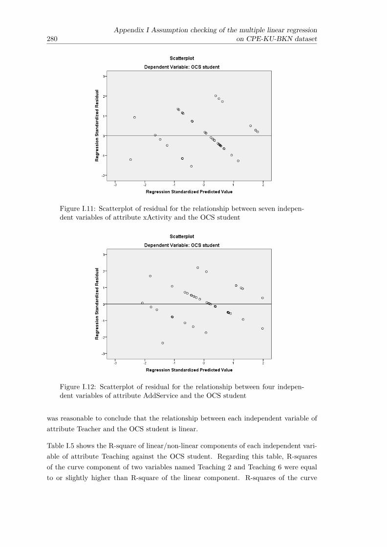
280Appendix I Assumption checking of the multiple linear regression
on CPE-KU-BKN dataset
Figure I.11: Scatterplot of residual for the relationship between seven indepen-dent variables of attribute xActivity and the OCS student
Figure I.12: Scatterplot of residual for the relationship between four indepen-dent variables of attribute AddService and the OCS student
was reasonable to conclude that the relationship between each independent variable ofattribute Teacher and the OCS student is linear.
Table I.5 shows the R-square of linear/non-linear components of each independent vari-able of attribute Teaching against the OCS student. Regarding this table, R-squaresof the curve component of two variables named Teaching 2 and Teaching 6 were equalto or slightly higher than R-square of the linear component. R-squares of the curve

Appendix I Assumption checking of the multiple linear regressionon CPE-KU-BKN dataset 281
Table I.3: R-square of the components of regression equation (attribute Teacher)
Independent variable R-SquareLinear Quadratic Cubic
Teacher 1 0.206 0.206 0.206Teacher 2 0.205 0.209 0.209Teacher 3 0.214 0.215 0.215Teacher 4 0.163 0.174 0.179Teacher 5 0.147 0.151 0.151
Table I.4: Chi-square statistic for the difference test of equality of correlations(attribute Teacher)
Independent variable χ2 df p-value EqualityTeacher 1 0.000 2 1.000 YesTeacher 2 0.001 2 1.000 YesTeacher 3 0.000 2 1.000 YesTeacher 4 0.011 2 0.994 YesTeacher 5 0.001 2 1.000 Yes
component of the other four variables named Teaching1, and Teaching 3-5 were greatlyhigher than R-squares of the linear component indicated a sign of non-linearity.
However, considering the test for equality of several independent correlation coefficientsreported in Table I.6, it showed that there was no significant difference among corre-lations of the linear/non-linear components for each independent variable of attributeTeaching. Therefore, it was reasonable to conclude that the relationship between eachindependent variable of attribute Teaching and the OCS student is linear.
Table I.5: R-square of the components of regression equation (attribute Teach-ing)
Independent variable R-SquareLinear Quadratic Cubic
Teaching 1 0.461 0.480 0.483Teaching 2 0.024 0.028 0.028Teaching 3 0.162 0.190 0.196Teaching 4 0.023 0.032 0.032Teaching 5 0.253 0.264 0.286Teaching 6 0.116 0.119 0.119
Table I.7 shows the R-square of linear/non-linear components of each independent vari-able of attribute Admin against the OCS student. Regarding this table, R-squares ofthe curve component of most variables were equal to or slightly higher than R-squareof the linear component. Only the variable named Admin 5 which its R-squares of thecurve component were greatly higher than its R-squares of the linear component.
Given R-square from Table I.7, the test for equality of several independent correlationcoefficients was conducted and the result was reported in Table I.8. The Table I.8 showed

282Appendix I Assumption checking of the multiple linear regression
on CPE-KU-BKN dataset
Table I.6: Chi-square statistic for the difference test of equality of correlations(attribute Teaching)
Independent variable χ2 df p-value EqualityTeaching 1 0.022 2 0.989 YesTeaching 2 0.004 2 0.998 YesTeaching 3 0.055 2 0.973 YesTeaching 4 0.021 2 0.990 YesTeaching 5 0.039 2 0.981 YesTeaching 6 0.001 2 1.000 Yes
that there was no significant difference among correlations of the linear/non-linear com-ponents for each independent variable of attribute Admin. Therefore, it was reasonableto conclude that the relationship between each independent variable of attribute Adminand the OCS student is linear.
Table I.7: R-square of the components of regression equation (attribute Admin)
Independent variable R-SquareLinear Quadratic Cubic
Admin 1 0.045 0.046 0.046Admin 2 0.060 0.064 0.064Admin 3 0.003 0.003 0.003Admin 4 0.003 0.003 0.004Admin 5 0.068 0.105 0.105
Table I.8: Chi-square statistic for the difference test of equality of correlations(attribute Admin)
Independent variable χ2 df p-value EqualityAdmin 1 0.000 2 1.000 YesAdmin 2 0.002 2 0.999 YesAdmin 3 0.000 2 1.000 YesAdmin 4 0.002 2 0.999 YesAdmin 5 0.128 2 0.938 Yes
Table I.9 shows the R-square of linear/non-linear components of each independent vari-able of attribute CompFac against the OCS student. Regarding this table, R-squares ofthe curve component of most variables were equal to or slightly higher than R-squareof the linear component. Only the variable named CompFac 1 which its R-squares ofthe curve component were critically higher than its R-squares of the linear componentindicated a sign of non-linearity.
However, considering the test for equality of several independent correlation coefficientsreported in Table I.10, it showed that there was no significant difference among corre-lations of the linear/non-linear components for each independent variable of attributeCompFac. Therefore, it was reasonable to conclude that the relationship between eachindependent variable of attribute CompFac and the OCS student is linear.

Appendix I Assumption checking of the multiple linear regressionon CPE-KU-BKN dataset 283
Table I.9: R-square of the components of regression equation (attribute Comp-Fac)
Independent variable R-SquareLinear Quadratic Cubic
CompFac 1 0.005 0.163 0.188CompFac 2 0.080 0.080 0.094CompFac 3 0.057 0.079 0.079CompFac 4 0.025 0.037 0.038
Table I.10: Chi-square statistic for the difference test of equality of correlations(attribute CompFac)
Independent variable χ2 df p-value EqualityCompFac 1 3.784 2 0.151 YesCompFac 2 0.018 2 0.991 YesCompFac 3 0.055 2 0.973 YesCompFac 4 0.036 2 0.982 Yes
Table I.11 shows the R-square of linear/non-linear components of each independentvariable of attribute xActivity against the OCS student. Regarding this table, R-squaresof the curve component of most variables were equal to or slightly higher than R-squareof the linear component. Only the variables named xActivity 1 and xActivity 4 whichtheir R-squares of the curve component were critically higher than their R-squares ofthe linear component indicated a sign of non-linearity.
However, considering the test for equality of several independent correlation coefficientsreported in Table I.12, it showed that there was no significant difference among cor-relations of the linear/non-linear component for each independent variable of attributexActivity. Therefore, it was reasonable to conclude that the relationship between eachindependent variable of attribute xActivity and the OCS student is linear.
Table I.11: R-square of the components of regression equation (attribute xAc-tivity)
Independent variable R-SquareLinear Quadratic Cubic
xActivity 1 0.105 0.318 0.477xActivity 2 0.438 0.451 0.451xActivity 3 0.155 0.170 0.179xActivity 4 0.018 0.225 0.225xActivity 5 0.376 0.381 0.381xActivity 6 0.293 0.319 0.327xActivity 7 0.310 0.329 0.350
Table I.13 shows the R-square of linear/non-linear component of each independent vari-able of attribute AddService against the OCS student. Regarding this table, R-squares

284Appendix I Assumption checking of the multiple linear regression
on CPE-KU-BKN dataset
Table I.12: Chi-square statistic for the difference test of equality of correlations(attribute xActivity)
Independent variable χ2 df p-value EqualityxActivity 1 5.321 2 0.070 YesxActivity 2 0.008 2 0.996 YesxActivity 3 0.025 2 0.987 YesxActivity 4 3.864 2 0.145 YesxActivity 5 0.001 2 0.999 YesxActivity 6 0.043 2 0.979 YesxActivity 7 0.054 2 0.973 Yes
of the curve component of all variables were greatly higher than R-square of the linearcomponent indicated a sign of non-linearity.
However, considering the test for equality of several independent correlation coefficientsreported in Table I.14, it showed that there was no significant difference among corre-lations of the linear/non-linear components for each independent variable of attributeAddService. Therefore, it was reasonable to conclude that the relationship between eachindependent variable of attribute AddService and the OCS student is linear.
Table I.13: R-square of the components of regression equation (attributeAddService)
Independent variable R-SquareLinear Quadratic Cubic
AddService 1 0.091 0.145 0.146AddService 2 0.171 0.174 0.224AddService 3 0.368 0.368 0.382AddService 4 0.150 0.162 0.172
Table I.14: Chi-square statistic for the difference test of equality of correlations(attribute AddService)
Independent variable χ2 df p-value EqualityAddService 1 0.218 2 0.897 YesAddService 2 0.140 2 0.933 YesAddService 3 0.009 2 0.996 YesAddService 4 0.021 2 0.989 Yes
In summary, the test of the addition of curve components of all variables in each groupsuggested that the linearity assumption was met.
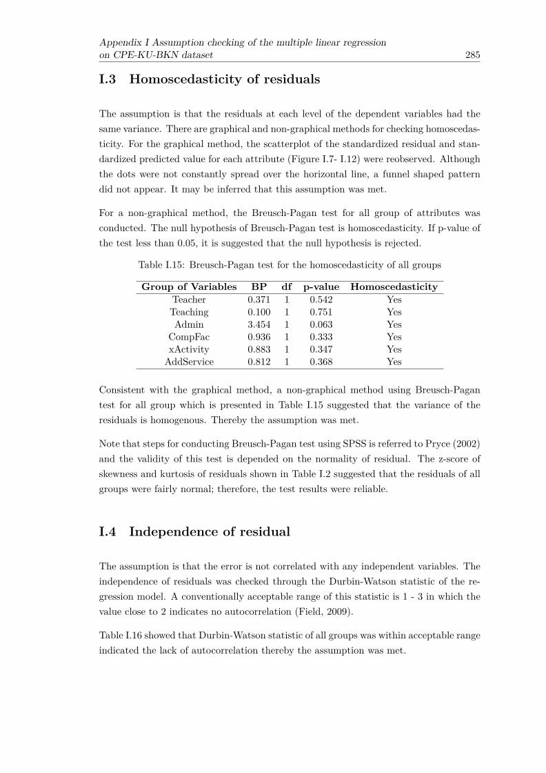
Appendix I Assumption checking of the multiple linear regressionon CPE-KU-BKN dataset 285
I.3 Homoscedasticity of residuals
The assumption is that the residuals at each level of the dependent variables had thesame variance. There are graphical and non-graphical methods for checking homoscedas-ticity. For the graphical method, the scatterplot of the standardized residual and stan-dardized predicted value for each attribute (Figure I.7- I.12) were reobserved. Althoughthe dots were not constantly spread over the horizontal line, a funnel shaped patterndid not appear. It may be inferred that this assumption was met.
For a non-graphical method, the Breusch-Pagan test for all group of attributes wasconducted. The null hypothesis of Breusch-Pagan test is homoscedasticity. If p-value ofthe test less than 0.05, it is suggested that the null hypothesis is rejected.
Table I.15: Breusch-Pagan test for the homoscedasticity of all groups
Group of Variables BP df p-value HomoscedasticityTeacher 0.371 1 0.542 YesTeaching 0.100 1 0.751 YesAdmin 3.454 1 0.063 Yes
CompFac 0.936 1 0.333 YesxActivity 0.883 1 0.347 YesAddService 0.812 1 0.368 Yes
Consistent with the graphical method, a non-graphical method using Breusch-Pagantest for all group which is presented in Table I.15 suggested that the variance of theresiduals is homogenous. Thereby the assumption was met.
Note that steps for conducting Breusch-Pagan test using SPSS is referred to Pryce (2002)and the validity of this test is depended on the normality of residual. The z-score ofskewness and kurtosis of residuals shown in Table I.2 suggested that the residuals of allgroups were fairly normal; therefore, the test results were reliable.
I.4 Independence of residual
The assumption is that the error is not correlated with any independent variables. Theindependence of residuals was checked through the Durbin-Watson statistic of the re-gression model. A conventionally acceptable range of this statistic is 1 - 3 in which thevalue close to 2 indicates no autocorrelation (Field, 2009).
Table I.16 showed that Durbin-Watson statistic of all groups was within acceptable rangeindicated the lack of autocorrelation thereby the assumption was met.
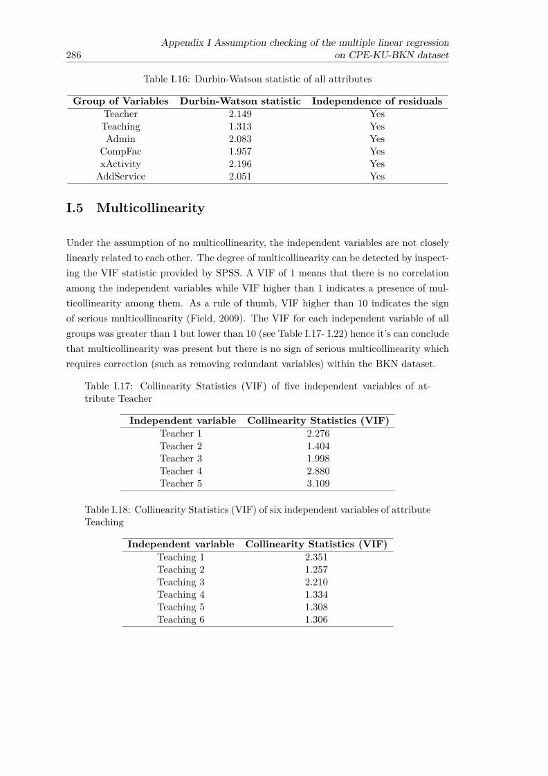
286Appendix I Assumption checking of the multiple linear regression
on CPE-KU-BKN dataset
Table I.16: Durbin-Watson statistic of all attributes
Group of Variables Durbin-Watson statistic Independence of residualsTeacher 2.149 YesTeaching 1.313 YesAdmin 2.083 Yes
CompFac 1.957 YesxActivity 2.196 YesAddService 2.051 Yes
I.5 Multicollinearity
Under the assumption of no multicollinearity, the independent variables are not closelylinearly related to each other. The degree of multicollinearity can be detected by inspect-ing the VIF statistic provided by SPSS. A VIF of 1 means that there is no correlationamong the independent variables while VIF higher than 1 indicates a presence of mul-ticollinearity among them. As a rule of thumb, VIF higher than 10 indicates the signof serious multicollinearity (Field, 2009). The VIF for each independent variable of allgroups was greater than 1 but lower than 10 (see Table I.17- I.22) hence it’s can concludethat multicollinearity was present but there is no sign of serious multicollinearity whichrequires correction (such as removing redundant variables) within the BKN dataset.
Table I.17: Collinearity Statistics (VIF) of five independent variables of at-tribute Teacher
Independent variable Collinearity Statistics (VIF)Teacher 1 2.276Teacher 2 1.404Teacher 3 1.998Teacher 4 2.880Teacher 5 3.109
Table I.18: Collinearity Statistics (VIF) of six independent variables of attributeTeaching
Independent variable Collinearity Statistics (VIF)Teaching 1 2.351Teaching 2 1.257Teaching 3 2.210Teaching 4 1.334Teaching 5 1.308Teaching 6 1.306

Appendix I Assumption checking of the multiple linear regressionon CPE-KU-BKN dataset 287
Table I.19: Collinearity Statistics (VIF) of five independent variables of at-tribute Admin
Independent variable Collinearity Statistics (VIF)Admin 1 1.884Admin 2 2.409Admin 3 2.792Admin 4 3.180Admin 5 2.554
Table I.20: Collinearity Statistics (VIF) of four independent variables of at-tribute CompFac
Independent variable Collinearity Statistics (VIF)CompFac 1 2.526CompFac 2 1.963CompFac 3 1.252CompFac 4 1.604
Table I.21: Collinearity Statistics (VIF) of seven independent variables of at-tribute xActivity
Independent variable Collinearity Statistics (VIF)xActivity 1 2.592xActivity 2 2.239xActivity 3 4.033xActivity 4 3.551xActivity 5 2.683xActivity 6 3.070xActivity 7 3.193
Table I.22: Collinearity Statistics (VIF) of four independent variables of at-tribute AddService
Independent variable Collinearity Statistics (VIF)AddService 1 1.866AddService 2 2.238AddService 3 1.194AddService 4 1.912


Appendix J
Staff evaluation of SWOT surveymaterial
J.1 Survey on the level of agreement toward SWOT of de-partment
This survey forms part of a study into the development of SWOT based on customersatisfaction survey, in particular the case study consider Department of Computer En-gineering, Faculty of Engineering at Kamphaeng Saen, Kasetsart University (CPE-KU-KPS). Definition of each aspect of SWOT is provided as follow:Strengths refer to the internal operation that the department doing wellWeakness refer to the internal operation that the department poorly performOpportunities refer to external factors that the department can use its advantage oroperation that department perform better than other departments in Kasetsart Univer-sity.Threats refer to external factors that may cause a problem to the department or op-eration that department poorly perform than other departments in Kasetsart University.
Section I. Strength-Weakness.This section asks about your level of agreement towards the strengths and weaknesses ofthe CPE-KU-KPS that have been identified based on an earlier CPE-KU-KPS’s studentsatisfaction survey.
Instruction: Please assess your level of agreement with the following sentences accord-ing to your view and experience by ticking the appropriate response using the followingscales:
289

290 Appendix J Staff evaluation of SWOT survey material
Score Interpretation on Level of Agreement4 Completely agree3 Agree2 Disagree1 Completely disagree
Section II. Opportunity-Threat.This section asks about your level of agreement towards the opportunities and threats inthe CPE-KU-KPS that identified by comparing the CPE-KU-KPS’s student satisfactionwith the Department of Computer Engineering, Kasetsart University, Bangkhen campus(CPE-KU-BKN)’s student satisfaction.
Instruction: Please assess your level of agreement with the following sentences accord-ing to your view and experience by ticking the appropriate response.
Section III. Personal Information
Instruction: Please tick the circle that best corresponds to your answer for each ques-tion below
1. Gender ⃝ Male ⃝ Female
2. Number of working years at CPE-KU-KPS ⃝ <1 ⃝ 1-3 ⃝ 4-6 ⃝ 7-10 ⃝>10
3. Position ⃝ Academic staff ⃝ Non-Academic staff
Thank you very much for your help

Appendix J Staff evaluation of SWOT survey material 291
Senten
cesab
outstreng
thsan
dwe
akne
sses
Levelo
fAgreement
43
21
1.Te
aching
ability
ofteaching
staff
isastreng
thof
thede
partment
2.Su
bjectexpe
rtise
ofteaching
staff
isastreng
thof
thede
partment
3.Friend
linessof
theteaching
staff
towa
rdsstud
ents
isastreng
thof
thede
partment
4.Abilityof
teaching
staff
togive
advice
andsupp
ortto
stud
entlearning
isastreng
thof
thede
partment
5.App
ropriate
numbe
rof
stud
ents
perclassis
astreng
thof
thede
partment
6.Kno
wledg
eof
rulesan
dproced
ures
ofno
n-acad
emic
staff
mem
bers
isastreng
thof
thede
partment
7.Kno
wledg
eof
theinform
ationab
outcourses,
exam
san
dactiv
ities
ofno
n-acad
emic
staff
mem
bers
isastreng
thof
thede
partment
8.Po
orqu
ality
ofcompu
terfacilitiesforstud
ents
(Hardw
arean
dSo
ftware)
isawe
akne
ssof
thede
partment
9.La
ckof
availabilityof
compu
terfacilitiesforstud
ents
isawe
akne
ssof
thede
partment
10.La
ckof
availabilityof
printin
gan
dph
otocop
ying
facilitiesis
awe
akne
ssof
thede
partment
11.Po
orarrang
ementof
cultu
rale
xcha
ngeprog
ramswith
foreigncoun
triesis
awe
akne
ssof
thede
partment
12.Po
orarrang
ementof
health
developm
entactiv
ities
isawe
akne
ssof
thede
partment
13.La
ckof
finan
cial
aidprov
ided
forstud
ents
isawe
akne
ssof
thede
partment
14.La
ckof
med
ical
supp
ortprov
ided
forstud
ents
isawe
akne
ssof
thede
partment
15.La
ckof
availabilityof
library
facilitiesis
awe
akness
ofthede
partment

292 Appendix J Staff evaluation of SWOT survey material
Sentencesabout
opportunitiesand
threatsLevelofA
greement
43
21
1.Increasing
theavailability
ofteachingstaff
tothe
studentsis
anopportunity
forthe
department
2.Increasing
theavailability
oflecturematerials
isan
opportunityfor
thedepartm
ent3.
IncreasingE-learning
resourcesto
supportstudent
learningare
anopportunity
forthe
department
4.Increasing
theability
togive
clearand
timely
feedbackto
studentsis
anopportunity
forthe
department
5.Increasing
accurateand
up-to-datecourse
unitcontent
isan
opportunityfor
thedepartm
ent6.
Inadequateofteaching
facilitiesand
learningareas
isathreat
tothe
department
7.Lack
ofinterestin
solvingthe
students’problemby
non-academic
staffmem
bersis
athreat
tothe
department
8.Lack
offriendlinessofnon-academ
icstaff
mem
bersto
studentsis
athreat
tothe
department
9.Lack
ofabilityofnon-academ
icstaff
mem
berstoprovide
servicesinatim
elymannerisa
threattothe
department
10.Lack
ofavailabilityofinternet
accessfor
studentsis
athreat
tothe
department
11.Updated
contentand
easyto
findinform
ationon
thedepartm
entwebsite
isan
opportunityfor
thedepartm
ent12.
Improving
thearrangem
entoffield
tripsactivities
isan
opportunityfor
thedepartm
ent13.
Improving
thearrangem
entofm
oraldevelopment
activitiesis
anopportunity
forthe
department
14.Im
provingthe
arrangement
ofinterpersonalskillsdevelopm
entactivities
isan
opportunityfor
thedepartm
ent15.
Improving
thearrangem
entofpersonallearning
andthinking
skillsdevelopm
entactivities
isan
opportunityfor
thedepartm
ent16.
Improving
thearrangem
entofsocialvolunteer
activitiesis
anopportunity
forthe
department

Appendix J Staff evaluation of SWOT survey material 293
J.2 Participant Information sheet
Study Title: Mining Survey Data for SWOT analysis (validation phase I)Researcher: Boonyarat PhadermrodEthics number: ERGO/FPSE/18153
Please read this information carefully before deciding to take part in this research. Ifyou are happy to participate you will be asked to sign a consent form.
What is the research about?I am completing a PhD research about mining survey data for SWOT analysiswhich aimed to generate prioritized SWOT factors based on the customer’s per-ception. To evaluate the proficiency of the proposed approach in the real-worldsituation, the case study of Department of Computer Engineering (DoCE), Kaset-sart University will be conducted. Through this case study, your response onthe level of agreement with the SWOT aspects of the DoCE will be analysed toevaluate SWOT generated based on satisfaction survey.
Why have I been chosen?At this stage, this research is trying to get a level of agreement with the SWOT as-pects of the DoCE which generated based on student satisfaction survey of DoCE.Thus, you are chosen as you are staff members of DoCE, Kasetsart University.
What will happen to me if I take part?The questionnaire will take no longer than 15 minutes to complete. There arethree sections in the questionnaire. Section 1 and 2 asks about your level of agree-ment with Strength-Weakness and Opportunity-Threat of the DoCE respectively.Section 3 asks about your general information.
Are there any benefits in my taking part?By taking part, you have the opportunity to help us develop the new method togenerate SWOT based on satisfaction survey which can be used in government,academic institution and private company.
Are there any risks involved?There is no risk involved for participants completing the questionnaire.
Will my participation be confidential?The name of the participants will not be taken and participation will be keptanonymous. All data will be safe in a protected computer. All will be destroyedonce the research is completed.
What happens if I change my mind?You have the right to withdraw from doing the questionnaire at any time by exitingthe webpage.

294 Appendix J Staff evaluation of SWOT survey material
What happens if something goes wrong?If you have any concern or complaint with this research please contacts me (Boon-yarat Phadermrod: [email protected]). If you have a trouble with the on-line forms, please contact the ECS School Office on [email protected] 02380592909.
Where can I get more information?If you would like more information on this research please feel free to contact me(Boonyarat Phadermrod: [email protected])
J.3 Result of language consistency translation test of staffevaluation of SWOT survey
Remark: +1 the question/ instruction is consistent with the English version0 undecided about whether Thai question/ instruction is consistent with the
English version−1 the question/ instruction is not consistent with the English version

Appendix J Staff evaluation of SWOT survey material 295
TableJ.1:
Summaryof
lang
uage
consist
ency
tran
slatio
ntest
ofstaff
evalua
tionof
SWOT
survey
Que
stion/
Instruction
Que
stion/
Instruction
Lang
uage
consistenc
yscore
Total
Com
ment
(Eng
lish)
(Tha
i)Ex
pert
Expe
rtEx
pert
Score
12
31
This
questio
nnaire
form
spa
rtof
astud
yinto
thede
velopm
entof
SWOT
basedon
custom
ersatis
factionsurvey,
inpa
rticular
the
case
stud
yconsider
Dep
artm
entof
Com
puterEn
gine
ering,
Facu
ltyof
Engine
eringat
Kam
phaeng
Saen
,Kasetsart
universit
y(C
PE-K
U-
KPS
).
แบบป
ระเมน
นเปนส
วนหน
งของงาน
วจยเพ
อการ
สรางจ
ดแขง
จดออ
นโอกาสแล
ะอปส
รรค(
SWOT
)จาก
ผลสารวจค
วามพง
พอใจข
องลก
คาโด
ยกรณ
ศกษา
ในงาน
วจยน
คอภาคว
ชาวศ
วกรรมค
อมพว
เตอร
คณะวศว
กรรม
ศาสตร
กาแพ
งแสน
มหาวท
ยาลย
เกษตร
ศาสตร
(วศ.คอ
มกพส
)
+1
+1
+1
3Che
cktheprop
erwa
yto
usethewo
rdSW
OT
inTha
icon
text.
2Se
ctionI.Streng
th-W
eakn
ess.
ตอนท
1.ระดบ
ความคด
เหนตอ
จดแข
งและ
จดออ
นของภาคว
ชาวศ
วกรรมค
อมพว
เตอร
+1
+1
+1
3
3Thissection
asks
abou
tyo
urlevelof
agreem
enttowa
rdsthestreng
thsan
dwe
akne
sses
oftheCPE
-KU-K
PSthat
were
identifi
edba
sedon
anearlier
CPE
-KU-K
PS’s
stud
entsatis
factionsurvey.
แบบส
อบถามส
วนนส
ารวจถ
งระดบ
ความคด
เหนขอ
งทานต
อจดแ
ขง(St
rength
)แล
ะจดอ
อน(W
eaknes
s)ขอ
งภาควช
าวศวก
รรมค
อมพว
เตอรซ
งจดแข
งและ
จดออ
นของภาคว
ชาเหล
านสร
างขนจ
ากผล
การวเคร
าะหแบ
บประเมน
ความพง
พอใจข
องนส
ตตอภ
าควช
า
+1
+1
+1
3
4Instruction:
Please
assess
your
levelo
fag
reem
entwith
thefollo
wingsenten
ces
accordingto
your
view
andexpe
rienc
eby
ticking
theap
prop
riate
respon
se:
คาชแ
จง:กร
ณาระบร
ะดบค
วามคด
เหนขอ
งทาน
ตอขอ
ความดานล
างตามคว
ามคด
เหนแล
ะประสบ
การณ
จากการท
างานข
องทาน
ณภาคว
ชาวศ
วกรรม
คอมพ
วเตอร
โดยท
าเครองห
มายถ
ก(X)ในช
องทต
รงกบ
ระดบ
ความคด
เหนขอ
งทาน
+1
+1
+1
3
5Com
pletelyag
ree
เหนดว
ยอยาง
ยง+1
+1
+1
3Agree
เหนดว
ยDisa
gree
ไมเหน
ดวย
Com
pletelydisagree
ไมเหน
ดวยอ
ยางยง
6Te
aching
ability
ofteaching
staff
isa
streng
thof
thede
partment
ความสามารถ
ในการส
อนขอ
งอาจา
รยผส
อนถอ
เปนจด
แขงของภาคว
ชา+1
+1
+1
3
7Su
bjectexpe
rtise
ofteaching
staff
isa
streng
thof
thede
partment
ความเชย
วชาญ
ในเนอ
หาวช
าของอาจาร
ยผสอ
นถอ
เปนจด
แขงของภาคว
ชา+1
+1
+1
3

296 Appendix J Staff evaluation of SWOT survey material
Question/
InstructionQuestion/
InstructionLanguage
consistencyscore
TotalCom
ment
(English)(T
hai)Expert
ExpertExpert
Score1
23
8Friendliness
ofthe
teachingstaff
to-wards
studentsis
astrength
ofthede-
partment
ความเปนกนเองของอาจารยผสอนตอนสตถอเปนจดแขงของภาควชา
+1
+1
+1
3
9Ability
ofteaching
staffto
givead-
viceand
supportstudent
learningis
astrength
ofthedepartm
ent
การใหคาปรกษาและความชวยเหลอในการเรยนของอาจารยผสอนตอนสตถอเปนจดแขงของภาควชา
+1
+1
+1
3
10Appropriate
number
ofstudents
perclass
isastrength
ofthedepartm
entความเหมาะสมของจานวนนสตในชนเรยนถอเปน
จดแขงของภาควชา
+1
+1
+1
3
11Know
ledgeof
rulesand
proceduresof
non-academic
staffmem
bersis
astrength
ofthedepartm
ent
ความรเรองขอบงคบระเบยบมหาวทยาลยของเจา
หนาทถอเปนจดแขงของภาควชา+1
+1
+1
3Add
“ความชานาญ”into
statement
12Know
ledgeof
theinform
ationabout
courses,exam
sand
activitiesof
non-academ
icstaff
mem
bersisastrength
ofthe
department
ความรเรองขอมลขาวสารเกยวกบรายวชา
การสอบและ
กจกรรมนสตของเจาหนาทถอเปนจดแขงของ
ภาควชา
+1
+1
+1
3
13Poor
qualityof
computer
facilitiesfor
students(H
ardwareand
Software)is
aweakness
ofthedepartm
ent
อปกรณคอมพวเตอร(ฮารดแวรและซอฟตแวร)ทดอยคณภาพถอเปนจดออนของภาควชา
+1
+1
+1
3
14Lack
ofavailability
ofcom
puterfacil-
itiesfor
studentsis
aweakness
ofthe
department
การขาดความพรอมใหบรการของอปกรณคอมพวเตอรถอเปนจดออนของภาควชา
+1
+1
02
Rephrase
tomake
thestatem
entmore
clear
15Lack
ofavailabilityofprinting
andpho-
tocopyingfacilities
isaweakness
ofthedepartm
ent
การขาดความพรอมใหบรการของเครองพมพและเครองถายเอกสารถอเปนจดออนของภาควชา
+1
+1
02
Rephrase
tomake
thestatem
entmore
clear
16Poor
arrangement
ofculturalexchangeprogram
swith
foreigncountries
isa
weaknessofthe
department
การจดโครงการแลกเปลยนวฒนธรรมกบตางประเทศทดอยประสทธภาพถอเปนจดออนของภาควชา
+1
+1
+1
3
17Poor
arrangement
ofhealth
develop-ment
activitiesis
aweakness
ofthede-
partment
การจดกจกรรมพฒนาสขภาพทดอยประสทธภาพถอ
เปนจดออนของภาควชา+1
+1
+1
3

Appendix J Staff evaluation of SWOT survey material 297
Que
stion/
Instruction
Que
stion/
Instruction
Lang
uage
consistenc
yscore
Total
Com
ment
(Eng
lish)
(Tha
i)Ex
pert
Expe
rtEx
pert
Score
12
318
Lack
offin
ancial
aidprov
ided
forstu-
dentsis
awe
akne
ssof
thede
partment
ความชว
ยเหลอ
ดานก
ารเงน
แกนส
ตทไม
เพยงพ
อถอ
เปนจด
ออนข
องภาคว
ชา+1
+1
02
Rep
hraseto
mak
ethe
statem
entmoreclear
19La
ckof
med
ical
supp
ortprov
ided
for
stud
ents
isawe
akne
ssof
thede
part-
ment
การให
ความชว
ยเหลอ
ดานร
กษาพ
ยาบาลแก
นสตท
ไมเพย
งพอถ
อเปนจ
ดออน
ของภาควช
า+1
+1
02
Rep
hraseto
mak
ethe
statem
entmoreclear
20La
ckof
availabilityof
library
facilities
isawe
akne
ssof
thede
partment
การข
าดคว
ามพร
อมให
บรการข
องหอ
งสมด
ถอเปน
จดออ
นของภาคว
ชา+1
+1
+1
3
21Se
ctionII.O
pportunity-T
hreat.
ตอนท
2.ระดบ
ความคด
เหนตอ
โอกาสแ
ละอป
สรรค
ของภาควช
าวศวก
รรมค
อมพว
เตอร
+1
+1
+1
3
22Thissection
asks
abou
tyo
urlevelof
agreem
ent
towa
rds
the
oppo
rtun
ities
andthreatsin
theCPE
-KU-K
PSthat
identifi
edby
compa
ringtheCPE
-KU-
KPS
’sstud
ent
satis
faction
with
the
Dep
artm
entof
Com
puterEn
gine
ering,
Kasetsart
University
,Ba
ngkh
encam-
pus(
CPE
-KU-B
KN)’s
stud
ents
atisfac-
tion.
แบบส
อบถามส
วนน
สารวจถ
งระดบ
ความคด
เหนขอ
งทาน
ตอโอกาส
(Oppo
rtunity)
และอ
ปสรรค
(Threa
t)ของภาคว
ชาวศ
วกรรมค
อมพว
เตอรซ
งโอกาส
และอ
ปสรรค
ของภาควช
าเหลานส
รางขน
จากการ
เปรยบ
เทยบผ
ลการ
วเคราะ
หแบบ
ประเม
นความ
พงพอ
ใจของนส
ตวศ.ค
อมกพ
ส.ตอ
ภาคว
ชากบ
ผลการ
วเคราะ
หแบบ
ประเม
นความ
พงพอ
ใจของนส
ตภาค
วชาวศ
วกรรมค
อมพว
เตอร
คณะวศว
กรรม
ศาสตร
มหาวท
ยาลยเก
ษตรศาสตร
(วศ.คอ
มบางเ
ขน)ต
อภาค
วชา
+1
+1
+1
3
23Instruction:
Please
assess
your
levelo
fag
reem
entwith
thefollo
wingsenten
ces
accordingto
your
view
andexpe
rienc
eby
ticking
theap
prop
riate
respon
se.
คาชแ
จง:กร
ณาระบร
ะดบค
วามคด
เหนขอ
งทาน
ตอขอ
ความดานล
างตามคว
ามคด
เหนแล
ะประสบ
การณ
จากการท
างานข
องทาน
ณภาคว
ชาวศ
วกรรม
คอมพ
วเตอร
โดยท
าเครองห
มายถ
ก(X)ในช
องทต
รงกบ
ระดบ
ความคด
เหนขอ
งทาน
+1
+1
+1
3
24Increasin
gtheavailability
ofteaching
staff
tothestud
ents
isan
oppo
rtun
ityforthede
partment
การเพ
มโอก
าสใน
การให
นสตเข
าพบน
อกเวล
าเรยน
ของอาจา
รยผส
อนถอ
เปนโอกาสข
องภาคว
ชา+1
+1
+1
3
25Increasin
gthe
availability
oflecture
materials
isan
oppo
rtun
ityforthede
-pa
rtment
การเพ
มความ
พรอม
ของเอ
กสารป
ระกอ
บการเ
รยนก
ารสอ
นถอเป
นโอก
าสขอ
งภาควช
า+1
+1
+1
3
26Increasin
gE-
learning
resourcesto
sup-
port
stud
entlearning
arean
oppo
rtu-
nity
forthede
partment
การเพ
มสอก
ารเรยนร
อเลกท
รอนก
ส(e-Learn
ing)ท
สนบส
นนการเร
ยนขอ
งนสต
ถอเปน
โอกาสข
องภาค
วชา
+1
+1
+1
3

298 Appendix J Staff evaluation of SWOT survey material
Question/
InstructionQuestion/
InstructionLanguage
consistencyscore
TotalCom
ment
(English)(T
hai)Expert
ExpertExpert
Score1
23
27Increasing
theability
togive
clearand
timely
feedbackto
studentsisanoppor-
tunityfor
thedepartm
ent
การวดประเมนผลทชดเจนและไดรบแจงภายในเวลาทกาหนดถอเปนโอกาสของภาควชา
+1
+1
02
Change
theword
“ไดรบแจง”
to“แจงใหนสตทราบ”
28Increasing
accurateandup-to-dateunit
contentis
anopportunity
forthe
de-partm
ent
การเพมความถกตองและความทนสมยของเนอหาวชาทสอนถอเปนโอกาสของภาควชา
+1
+1
+1
3
29Inadequate
ofteaching
facilitiesand
learningareasisa
threattothe
depart-ment
อปกรณการเรยนการสอนและ
สภาพหองเรยนทไมเหมาะสมตอการเรยนการสอน
ถอเปนอปสรรคของ
ภาควชา
+1
+1
+1
3Cut
theword
“การเรยนการสอน”
tomake
state-ment
more
clear30
Lackofinterestin
solvingthe
students’problem
bynon-academ
icstaff
mem
-bers
isathreat
tothe
department
การขาดความใสใจในการแกปญหาใหแกนสตของเจาหนาทถอเปนอปสรรคของภาควชา
+1
+1
+1
3
31Lack
offriendliness
ofnon-academ
icstaff
mem
bersto
studentsis
athreat
tothe
department
การขาดความเปนกนเองของเจาหนาทถอเปน
อปสรรคของภาควชา+1
+1
+1
3Change
theword
“ความเปนกนเอง”
to“มนษย
สมพนธทด”32
Lackof
abilityof
non-academic
staffmem
berstoprovide
servicesinatim
elymanner
isathreat
tothe
department
การขาดความสามารถในการใหบรการนสตในระยะเวลา
ทเหมาะสมของเจาหนาทถอเปนอปสรรคของ
ภาควชา
+1
+1
+1
3
33Lack
ofavailabilityofinternetaccessfor
studentsis
athreat
tothe
department
การขาดความพรอมใหบรการเชอมตออนเตอรเนตถอ
เปนอปสรรคของภาควชา+1
+1
+1
3
34Updated
contentandeasy
tofind
infor-mation
onthe
departmentwebsite
isanopportunity
forthe
department
เวบไซตประจาภาควชาทมเนอหาทนสมยและ
สามารถคนหาขอมลไดงายถอเปนโอกาสของภาควชา+1
+1
+1
3
35Im
provingthe
arrangement
offield
tripsactivitiesisanopportunity
forthedepartm
ent
การพฒนาการจดกจกรรมทศนะศกษาดงานใหดขนถอเปนโอกาสของภาควชา
+1
+1
+1
3Change
theword
“พฒนา”to
“เพมประสทธภาพ”
andcut
theword
“ใหดขน”36
Improving
thearrangem
entof
moral
development
activitiesis
anopportu-
nityfor
thedepartm
ent
การพฒนาการจดกจกรรมพฒนาคณธรรมใหดขนถอ
เปนโอกาสของภาควชา+1
+1
+1
3Sam
eas
35

Appendix J Staff evaluation of SWOT survey material 299
Que
stion/
Instruction
Que
stion/
Instruction
Lang
uage
consistenc
yscore
Total
Com
ment
(Eng
lish)
(Tha
i)Ex
pert
Expe
rtEx
pert
Score
12
337
Improv
ingthearrang
emento
finterpe
r-sona
lskills
developm
enta
ctivities
isan
oppo
rtun
ityforthede
partment
การพ
ฒนาการจ
ดกจก
รรมพ
ฒนาความ
สมพน
ธระหว
างบคค
ลใหด
ขนถอ
เปนโอกาสข
องภาคว
ชา+1
+1
+1
3Sa
meas
35
38Im
prov
ingthearrang
emento
fpersona
llearning
and
thinking
skills
develop-
menta
ctivities
isan
oppo
rtun
ityfort
hede
partment
การพ
ฒนาการจ
ดกจก
รรมพ
ฒนาทกษ
ะการค
ดและ
การ
เรยนร
ใหดข
นถอเป
นโอก
าสขอ
งภาควช
า+1
+1
+1
3Sa
meas
35
39Im
prov
ing
the
arrang
ement
ofsocial
volunteeractiv
ities
isan
oppo
rtun
ityforthede
partment
การพ
ฒนาการจ
ดกจก
รรมเพ
อสงคมใหด
ขนถอ
เปนโอกาสข
องภาคว
ชา+1
+1
+1
3Sa
meas
35
40Se
ctionIII.Pe
rson
alInform
ation
ตอนท
3.ขอ
มลพน
ฐานเกย
วกบผ
ตอบแ
บบสอ
บถาม
+1
+1
+1
341
Instruction:
Please
tickthecircle
that
correspo
ndsto
your
answ
erforeach
questio
nbe
low
คาชแ
จง:กร
ณาทาเคร
องหม
ายถก(X
)ในว
งกลม
ทตรง
กบขอ
มลขอ
งทาน
มากท
สด+1
+1
+1
3
42Gen
der
◦Male
◦Fe
male
เพศ◦ชาย
◦หญ
ง+1
+1
+1
343
Num
berof
workingyearsat
CPE
-KU-
KPS
จานวน
ปททางาน
ณภาคว
ชาวศ
วกรรมค
อมพว
เตอร
+1
+1
+1
3
44Po
sition
◦Acade
mic
staff
◦Non
-Acade
mic
staff
ตาแห
นง◦อาจาร
ย◦เจา
หนาท
+1
+1
+1
3


Appendix K
Assumption checking of onesample t-test for staff evaluationon SWOT factor
There are 31 variables represented the level of agreement of CPE-KU-KPS staff towardsproduced SWOT factor which divided into 15 variables for strengths-weaknesses and16 for opportunities-threats (denoted as SW1−15, OT1−16 respectively). Before the onesample t-test was conducted, the assumptions of one sample t-test were tested on eachvariable and the results are shown in the following sections.
K.1 Result of the assumptions test of one sample t-test onstaff agreement level of SWOT factor
The one-sample t-test required three assumptions to be met as follows (Field, 2009):
Assumption 1: Variables should be interval/ ratio level.
All 31 variables represented the level of agreement of CPE-KU-KPS staff that weremeasured on a scale of 1 to 4. This assumption there was met.
Assumption 2: The data are independent.
Responses to the level of agreement of CPE-KU-KPS staff are independent becausethey come from a different person. This assumption there was met.
Assumption 3: Sampling distribution of the dataset is relatively normal.
The normality for each variable was tested by using Shapiro-Wilk in SPSS sincethe size of the dataset is smaller than 2000. A review of the Shapiro-Wilk test fornormality for variable SW1−15, OT1−16 are shown in Table K.1 - K.2 respectively.
301
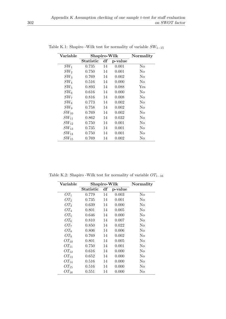
302Appendix K Assumption checking of one sample t-test for staff evaluation
on SWOT factor
Table K.1: Shapiro -Wilk test for normality of variable SW1−15
Variable Shapiro-Wilk NormalityStatistic df p-value
SW1 0.735 14 0.001 NoSW2 0.750 14 0.001 NoSW3 0.769 14 0.002 NoSW4 0.516 14 0.000 NoSW5 0.893 14 0.088 YesSW6 0.616 14 0.000 NoSW7 0.816 14 0.008 NoSW8 0.773 14 0.002 NoSW9 0.758 14 0.002 NoSW10 0.769 14 0.002 NoSW11 0.862 14 0.032 NoSW12 0.750 14 0.001 NoSW13 0.735 14 0.001 NoSW14 0.750 14 0.001 NoSW15 0.769 14 0.002 No
Table K.2: Shapiro -Wilk test for normality of variable OT1−16
Variable Shapiro-Wilk NormalityStatistic df p-value
OT1 0.779 14 0.003 NoOT2 0.735 14 0.001 NoOT3 0.639 14 0.000 NoOT4 0.801 14 0.005 NoOT5 0.646 14 0.000 NoOT6 0.810 14 0.007 NoOT7 0.850 14 0.022 NoOT8 0.806 14 0.006 NoOT9 0.769 14 0.002 NoOT10 0.801 14 0.005 NoOT11 0.750 14 0.001 NoOT12 0.616 14 0.000 NoOT13 0.652 14 0.000 NoOT14 0.516 14 0.000 NoOT15 0.516 14 0.000 NoOT16 0.551 14 0.000 No
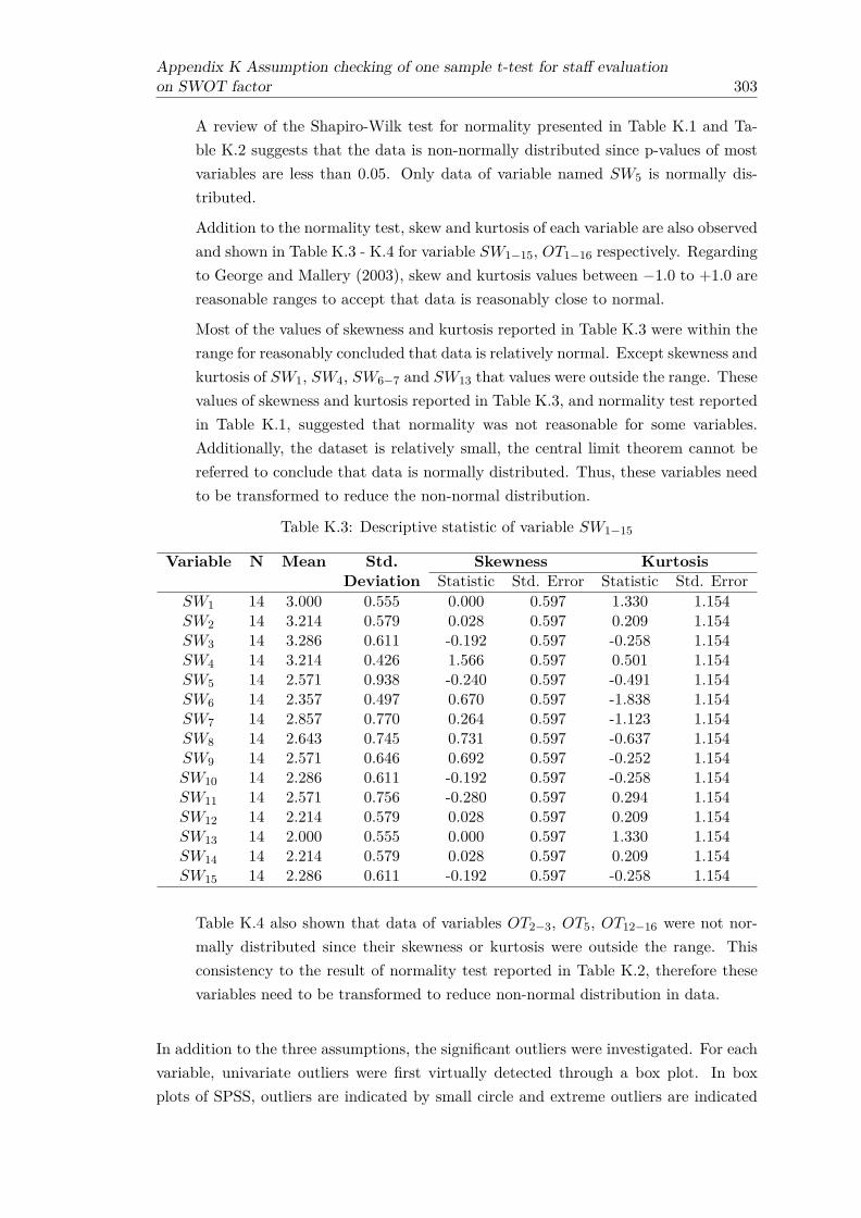
Appendix K Assumption checking of one sample t-test for staff evaluationon SWOT factor 303
A review of the Shapiro-Wilk test for normality presented in Table K.1 and Ta-ble K.2 suggests that the data is non-normally distributed since p-values of mostvariables are less than 0.05. Only data of variable named SW5 is normally dis-tributed.
Addition to the normality test, skew and kurtosis of each variable are also observedand shown in Table K.3 - K.4 for variable SW1−15, OT1−16 respectively. Regardingto George and Mallery (2003), skew and kurtosis values between −1.0 to +1.0 arereasonable ranges to accept that data is reasonably close to normal.
Most of the values of skewness and kurtosis reported in Table K.3 were within therange for reasonably concluded that data is relatively normal. Except skewness andkurtosis of SW1, SW4, SW6−7 and SW13 that values were outside the range. Thesevalues of skewness and kurtosis reported in Table K.3, and normality test reportedin Table K.1, suggested that normality was not reasonable for some variables.Additionally, the dataset is relatively small, the central limit theorem cannot bereferred to conclude that data is normally distributed. Thus, these variables needto be transformed to reduce the non-normal distribution.
Table K.3: Descriptive statistic of variable SW1−15
Variable N Mean Std. Skewness KurtosisDeviation Statistic Std. Error Statistic Std. Error
SW1 14 3.000 0.555 0.000 0.597 1.330 1.154SW2 14 3.214 0.579 0.028 0.597 0.209 1.154SW3 14 3.286 0.611 -0.192 0.597 -0.258 1.154SW4 14 3.214 0.426 1.566 0.597 0.501 1.154SW5 14 2.571 0.938 -0.240 0.597 -0.491 1.154SW6 14 2.357 0.497 0.670 0.597 -1.838 1.154SW7 14 2.857 0.770 0.264 0.597 -1.123 1.154SW8 14 2.643 0.745 0.731 0.597 -0.637 1.154SW9 14 2.571 0.646 0.692 0.597 -0.252 1.154SW10 14 2.286 0.611 -0.192 0.597 -0.258 1.154SW11 14 2.571 0.756 -0.280 0.597 0.294 1.154SW12 14 2.214 0.579 0.028 0.597 0.209 1.154SW13 14 2.000 0.555 0.000 0.597 1.330 1.154SW14 14 2.214 0.579 0.028 0.597 0.209 1.154SW15 14 2.286 0.611 -0.192 0.597 -0.258 1.154
Table K.4 also shown that data of variables OT2−3, OT5, OT12−16 were not nor-mally distributed since their skewness or kurtosis were outside the range. Thisconsistency to the result of normality test reported in Table K.2, therefore thesevariables need to be transformed to reduce non-normal distribution in data.
In addition to the three assumptions, the significant outliers were investigated. For eachvariable, univariate outliers were first virtually detected through a box plot. In boxplots of SPSS, outliers are indicated by small circle and extreme outliers are indicated
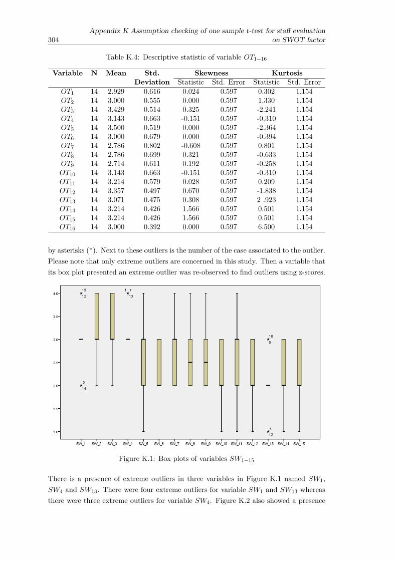
304Appendix K Assumption checking of one sample t-test for staff evaluation
on SWOT factor
Table K.4: Descriptive statistic of variable OT1−16
Variable N Mean Std. Skewness KurtosisDeviation Statistic Std. Error Statistic Std. Error
OT1 14 2.929 0.616 0.024 0.597 0.302 1.154OT2 14 3.000 0.555 0.000 0.597 1.330 1.154OT3 14 3.429 0.514 0.325 0.597 -2.241 1.154OT4 14 3.143 0.663 -0.151 0.597 -0.310 1.154OT5 14 3.500 0.519 0.000 0.597 -2.364 1.154OT6 14 3.000 0.679 0.000 0.597 -0.394 1.154OT7 14 2.786 0.802 -0.608 0.597 0.801 1.154OT8 14 2.786 0.699 0.321 0.597 -0.633 1.154OT9 14 2.714 0.611 0.192 0.597 -0.258 1.154OT10 14 3.143 0.663 -0.151 0.597 -0.310 1.154OT11 14 3.214 0.579 0.028 0.597 0.209 1.154OT12 14 3.357 0.497 0.670 0.597 -1.838 1.154OT13 14 3.071 0.475 0.308 0.597 2 .923 1.154OT14 14 3.214 0.426 1.566 0.597 0.501 1.154OT15 14 3.214 0.426 1.566 0.597 0.501 1.154OT16 14 3.000 0.392 0.000 0.597 6.500 1.154
by asterisks (*). Next to these outliers is the number of the case associated to the outlier.Please note that only extreme outliers are concerned in this study. Then a variable thatits box plot presented an extreme outlier was re-observed to find outliers using z-scores.
Figure K.1: Box plots of variables SW1−15
There is a presence of extreme outliers in three variables in Figure K.1 named SW1,SW4 and SW13. There were four extreme outliers for variable SW1 and SW13 whereasthere were three extreme outliers for variable SW4. Figure K.2 also showed a presence
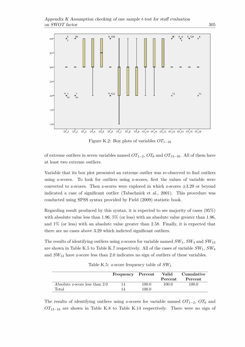
Appendix K Assumption checking of one sample t-test for staff evaluationon SWOT factor 305
Figure K.2: Box plots of variables OT1−16
of extreme outliers in seven variables named OT1−2, OT6 and OT13−16. All of them haveat least two extreme outliers.
Variable that its box plot presented an extreme outlier was re-observed to find outliersusing z-scores. To look for outliers using z-scores, first the values of variable wereconverted to z-scores. Then z-scores were explored in which z-scores ±3.29 or beyondindicated a case of significant outlier (Tabachnick et al., 2001). This procedure wasconducted using SPSS syntax provided by Field (2009) statistic book.
Regarding result produced by this syntax, it is expected to see majority of cases (95%)with absolute value less than 1.96, 5% (or less) with an absolute value greater than 1.96,and 1% (or less) with an absolute value greater than 2.58. Finally, it is expected thatthere are no cases above 3.29 which indicted significant outliers.
The results of identifying outliers using z-scores for variable named SW1, SW4 and SW13
are shown in Table K.5 to Table K.7 respectively. All of the cases of variable SW1, SW4
and SW13 have z-score less than 2.0 indicates no sign of outliers of these variables.
Table K.5: z-score frequency table of SW1
Frequency Percent Valid CumulativePercent Percent
Absolute z-score less than 2.0 14 100.0 100.0 100.0Total 14 100.0
The results of identifying outliers using z-scores for variable named OT1−2, OT6 andOT13−16 are shown in Table K.8 to Table K.14 respectively. There were no sign of

306Appendix K Assumption checking of one sample t-test for staff evaluation
on SWOT factor
Table K.6: z-score frequency table of SW4
Frequency Percent Valid CumulativePercent Percent
Absolute z-score less than 2.0 14 100.0 100.0 100.0Total 14 100.0
Table K.7: z-score frequency table of SW13
Frequency Percent Valid CumulativePercent Percent
Absolute z-score less than 2.0 14 100.0 100.0 100.0Total 14 100.0
outlier in five out of seven variables as these variables which are OT1−2, OT6, OT14−15
have z-score less than 2.0. Table K.11 and Table K.14 presented that there were somecases of variable OT13 and OT16 have z-score greater than 2.0 but still less than 3.29indicated that there were no significant outliers. Hence, outliers were not a problem ofthese two variables.
Table K.8: z-score frequency table of OT1
Frequency Percent Valid CumulativePercent Percent
Absolute z-score less than 2.0 14 100.0 100.0 100.0Total 14 100.0
Table K.9: z-score frequency table of OT2
Frequency Percent Valid CumulativePercent Percent
Absolute z-score less than 2.0 14 100.0 100.0 100.0Total 14 100.0
Table K.10: z-score frequency table of OT6
Frequency Percent Valid CumulativePercent Percent
Absolute z-score less than 2.0 14 100.0 100.0 100.0Total 14 100.0
Table K.11: z-score frequency table of OT13
Frequency Percent Valid CumulativePercent Percent
Absolute z-score less than 2.0 13 92.9 92.9 92.9Absolute z-score greater than 1.96 1 7.1 7.1 100.0Total 14 100.0

Appendix K Assumption checking of one sample t-test for staff evaluationon SWOT factor 307
Table K.12: z-score frequency table of OT14
Frequency Percent Valid CumulativePercent Percent
Absolute z-score less than 2.0 14 100.0 100.0 100.0Total 14 100.0
Table K.13: z-score frequency table of OT15
Frequency Percent Valid CumulativePercent Percent
Absolute z-score less than 2.0 14 100.0 100.0 100.0Total 14 100.0
Table K.14: z-score frequency table of OT16
Frequency Percent Valid CumulativePercent Percent
Absolute z-score less than 2.0 12 85.7 85.7 85.7Absolute z-score greater than 1.96 2 14.3 14.3 100.0Total 14 100.0
K.2 Result of the normality test for one sample t-test onthe transformed staff agreement level of SWOT factor
Although there was no sign of extreme outlier in data, some of variables in SW1−15
and OT1−16 were violated the normality assumption. Therefore, variables with skewedand peaked distribution need to be transformed, and others variables in SW1−15 andOT1−16 that have relatively normal distribution would also have to transform to be ableto compare with others that violate assumption.
As most data had positive skewness, Log, square root, and reciprocal function wereused to transform data. The results of normality test, skewness and kurtosis aftertransformed data using Log, square root, and reciprocal function are shown in Table K.15-K.18, Table K.19-K.22, Table K.23-K.26 respectively.
After transform data using the three functions, the data still did not have normal distri-bution. As p-value of normality test was less than 0.05 for all variables and there weresome variables that their skewness or kurtosis were outside the range. These variablesstill not met the assumptions of one-sample t-test therefore non-parametric test wasrecommended to be used instead of one-sample t-test.
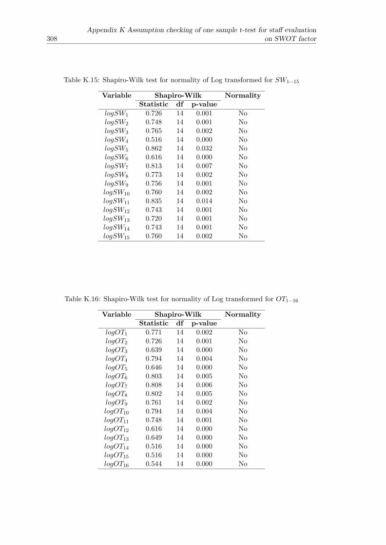
308Appendix K Assumption checking of one sample t-test for staff evaluation
on SWOT factor
Table K.15: Shapiro-Wilk test for normality of Log transformed for SW1−15
Variable Shapiro-Wilk NormalityStatistic df p-value
logSW1 0.726 14 0.001 NologSW2 0.748 14 0.001 NologSW3 0.765 14 0.002 NologSW4 0.516 14 0.000 NologSW5 0.862 14 0.032 NologSW6 0.616 14 0.000 NologSW7 0.813 14 0.007 NologSW8 0.773 14 0.002 NologSW9 0.756 14 0.001 NologSW10 0.760 14 0.002 NologSW11 0.835 14 0.014 NologSW12 0.743 14 0.001 NologSW13 0.720 14 0.001 NologSW14 0.743 14 0.001 NologSW15 0.760 14 0.002 No
Table K.16: Shapiro-Wilk test for normality of Log transformed for OT1−16
Variable Shapiro-Wilk NormalityStatistic df p-value
logOT1 0.771 14 0.002 NologOT2 0.726 14 0.001 NologOT3 0.639 14 0.000 NologOT4 0.794 14 0.004 NologOT5 0.646 14 0.000 NologOT6 0.803 14 0.005 NologOT7 0.808 14 0.006 NologOT8 0.802 14 0.005 NologOT9 0.761 14 0.002 NologOT10 0.794 14 0.004 NologOT11 0.748 14 0.001 NologOT12 0.616 14 0.000 NologOT13 0.649 14 0.000 NologOT14 0.516 14 0.000 NologOT15 0.516 14 0.000 NologOT16 0.544 14 0.000 No

Appendix K Assumption checking of one sample t-test for staff evaluationon SWOT factor 309
Table K.17: Descriptive statistic of Log transformed for SW1−15
Variable N Mean Std. Skewness KurtosisDeviation Statistic Std. Error Statistic Std. Error
logSW1 14 0.598 0.062 -0.561 0.597 1.461 1.154logSW2 14 0.621 0.061 -0.444 0.597 1.283 1.154logSW3 14 0.628 0.065 -0.597 0.597 0.863 1.154logSW4 14 0.623 0.041 1.566 0.597 0.501 1.154logSW5 14 0.537 0.125 -0.784 0.597 0.027 1.154logSW6 14 0.522 0.062 0.670 0.597 -1.838 1.154logSW7 14 0.578 0.087 0.027 0.597 -1.351 1.154logSW8 14 0.553 0.085 0.522 0.597 -1.174 1.154logSW9 14 0.547 0.076 0.453 0.597 -1.082 1.154logSW10 14 0.509 0.085 -0.761 0.597 1.367 1.154logSW11 14 0.543 0.100 -0.936 0.597 1.371 1.154logSW12 14 0.500 0.081 -0.633 0.597 1.777 1.154logSW13 14 0.470 0.084 -0.746 0.597 1.563 1.154logSW14 14 0.500 0.081 -0.633 0.597 1.777 1.154logSW15 14 0.509 0.085 -0.761 0.597 1.367 1.154
Table K.18: Descriptive statistic of Log transformed for OT1−16
Variable N Mean Std. Skewness KurtosisDeviation Statistic Std. Error Statistic Std. Error
logOT1 14 0.589 0.070 -0.409 0.597 0.104 1.154logOT2 14 0.598 0.062 -0.561 0.597 1.461 1.154logOT3 14 0.644 0.050 0.325 0.597 -2.241 1.154logOT4 14 0.612 0.072 -0.544 0.597 0.207 1.154logOT5 14 0.651 0.050 0.000 0.597 -2.364 1.154logOT6 14 0.596 0.076 -0.367 0.597 -0.350 1.154logOT7 14 0.568 0.104 -1.315 0.597 2.374 1.154logOT8 14 0.571 0.080 0.034 0.597 -1.084 1.154logOT9 14 0.564 0.072 -0.108 0.597 -0.966 1.154logOT10 14 0.612 0.072 -0.544 0.597 0.207 1.154logOT11 14 0.621 0.061 -0.444 0.597 1.283 1.154logOT12 14 0.637 0.048 0.670 0.597 -1.838 1.154logOT13 14 0.607 0.051 -0.425 0.597 3.785 1.154logOT14 14 0.623 0.041 1.566 0.597 0.501 1.154logOT15 14 0.623 0.041 1.566 0.597 0.501 1.154logOT16 14 0.600 0.044 -0.950 0.597 6.932 1.154
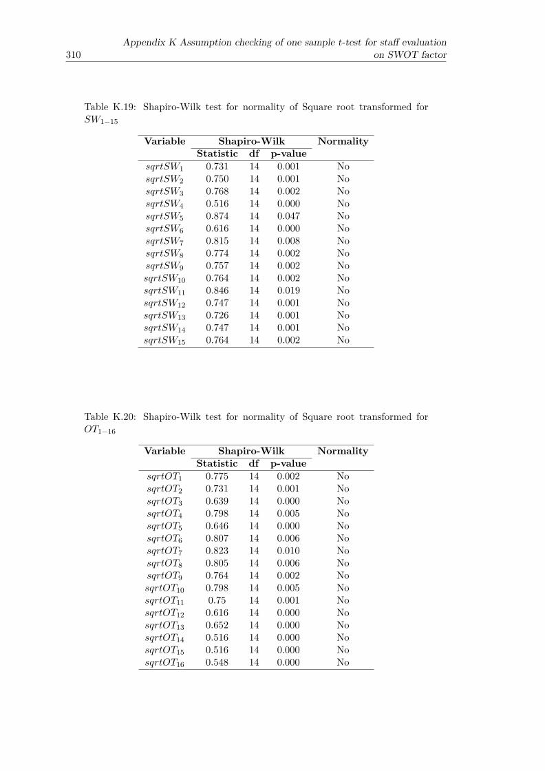
310Appendix K Assumption checking of one sample t-test for staff evaluation
on SWOT factor
Table K.19: Shapiro-Wilk test for normality of Square root transformed forSW1−15
Variable Shapiro-Wilk NormalityStatistic df p-value
sqrtSW1 0.731 14 0.001 NosqrtSW2 0.750 14 0.001 NosqrtSW3 0.768 14 0.002 NosqrtSW4 0.516 14 0.000 NosqrtSW5 0.874 14 0.047 NosqrtSW6 0.616 14 0.000 NosqrtSW7 0.815 14 0.008 NosqrtSW8 0.774 14 0.002 NosqrtSW9 0.757 14 0.002 NosqrtSW10 0.764 14 0.002 NosqrtSW11 0.846 14 0.019 NosqrtSW12 0.747 14 0.001 NosqrtSW13 0.726 14 0.001 NosqrtSW14 0.747 14 0.001 NosqrtSW15 0.764 14 0.002 No
Table K.20: Shapiro-Wilk test for normality of Square root transformed forOT1−16
Variable Shapiro-Wilk NormalityStatistic df p-value
sqrtOT1 0.775 14 0.002 NosqrtOT2 0.731 14 0.001 NosqrtOT3 0.639 14 0.000 NosqrtOT4 0.798 14 0.005 NosqrtOT5 0.646 14 0.000 NosqrtOT6 0.807 14 0.006 NosqrtOT7 0.823 14 0.010 NosqrtOT8 0.805 14 0.006 NosqrtOT9 0.764 14 0.002 NosqrtOT10 0.798 14 0.005 NosqrtOT11 0.75 14 0.001 NosqrtOT12 0.616 14 0.000 NosqrtOT13 0.652 14 0.000 NosqrtOT14 0.516 14 0.000 NosqrtOT15 0.516 14 0.000 NosqrtOT16 0.548 14 0.000 No
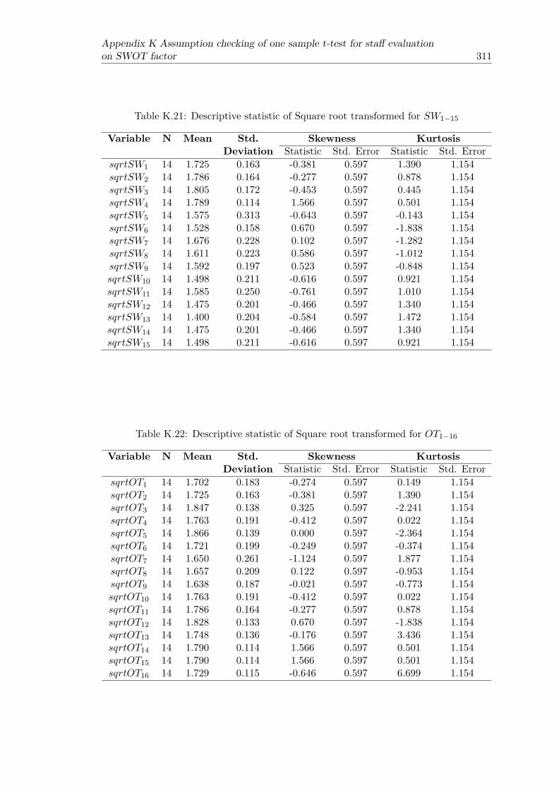
Appendix K Assumption checking of one sample t-test for staff evaluationon SWOT factor 311
Table K.21: Descriptive statistic of Square root transformed for SW1−15
Variable N Mean Std. Skewness KurtosisDeviation Statistic Std. Error Statistic Std. Error
sqrtSW1 14 1.725 0.163 -0.381 0.597 1.390 1.154sqrtSW2 14 1.786 0.164 -0.277 0.597 0.878 1.154sqrtSW3 14 1.805 0.172 -0.453 0.597 0.445 1.154sqrtSW4 14 1.789 0.114 1.566 0.597 0.501 1.154sqrtSW5 14 1.575 0.313 -0.643 0.597 -0.143 1.154sqrtSW6 14 1.528 0.158 0.670 0.597 -1.838 1.154sqrtSW7 14 1.676 0.228 0.102 0.597 -1.282 1.154sqrtSW8 14 1.611 0.223 0.586 0.597 -1.012 1.154sqrtSW9 14 1.592 0.197 0.523 0.597 -0.848 1.154sqrtSW10 14 1.498 0.211 -0.616 0.597 0.921 1.154sqrtSW11 14 1.585 0.250 -0.761 0.597 1.010 1.154sqrtSW12 14 1.475 0.201 -0.466 0.597 1.340 1.154sqrtSW13 14 1.400 0.204 -0.584 0.597 1.472 1.154sqrtSW14 14 1.475 0.201 -0.466 0.597 1.340 1.154sqrtSW15 14 1.498 0.211 -0.616 0.597 0.921 1.154
Table K.22: Descriptive statistic of Square root transformed for OT1−16
Variable N Mean Std. Skewness KurtosisDeviation Statistic Std. Error Statistic Std. Error
sqrtOT1 14 1.702 0.183 -0.274 0.597 0.149 1.154sqrtOT2 14 1.725 0.163 -0.381 0.597 1.390 1.154sqrtOT3 14 1.847 0.138 0.325 0.597 -2.241 1.154sqrtOT4 14 1.763 0.191 -0.412 0.597 0.022 1.154sqrtOT5 14 1.866 0.139 0.000 0.597 -2.364 1.154sqrtOT6 14 1.721 0.199 -0.249 0.597 -0.374 1.154sqrtOT7 14 1.650 0.261 -1.124 0.597 1.877 1.154sqrtOT8 14 1.657 0.209 0.122 0.597 -0.953 1.154sqrtOT9 14 1.638 0.187 -0.021 0.597 -0.773 1.154sqrtOT10 14 1.763 0.191 -0.412 0.597 0.022 1.154sqrtOT11 14 1.786 0.164 -0.277 0.597 0.878 1.154sqrtOT12 14 1.828 0.133 0.670 0.597 -1.838 1.154sqrtOT13 14 1.748 0.136 -0.176 0.597 3.436 1.154sqrtOT14 14 1.790 0.114 1.566 0.597 0.501 1.154sqrtOT15 14 1.790 0.114 1.566 0.597 0.501 1.154sqrtOT16 14 1.729 0.115 -0.646 0.597 6.699 1.154

312Appendix K Assumption checking of one sample t-test for staff evaluation
on SWOT factor
Table K.23: Shapiro-Wilk test for normality of Reciprocal transformed forSW1−15
Variable Shapiro-Wilk NormalityStatistic df p-value
newSW1 0.681 14 0.000 NonewSW2 0.706 14 0.000 NonewSW3 0.722 14 0.001 NonewSW4 0.516 14 0.000 NonewSW5 0.720 14 0.001 NonewSW6 0.616 14 0.000 NonewSW7 0.787 14 0.003 NonewSW8 0.758 14 0.002 NonewSW9 0.737 14 0.001 NonewSW10 0.648 14 0.000 NonewSW11 0.684 14 0.000 NonewSW12 0.632 14 0.000 NonewSW13 0.623 14 0.000 NonewSW14 0.632 14 0.000 NonewSW15 0.648 14 0.000 No
Table K.24: Shapiro-Wilk test for normality of Reciprocal transformed forOT1−16
Variable Shapiro-Wilk NormalityStatistic df p-value
newOT1 0.729 14 0.001 NonewOT2 0.681 14 0.000 NonewOT3 0.639 14 0.000 NonewOT4 0.749 14 0.001 NonewOT5 0.646 14 0.000 NonewOT6 0.762 14 0.002 NonewOT7 0.638 14 0.000 NonewOT8 0.773 14 0.002 NonewOT9 0.733 14 0.001 NonewOT10 0.749 14 0.001 NonewOT11 0.706 14 0.000 NonewOT12 0.616 14 0.000 NonewOT13 0.606 14 0.000 NonewOT14 0.516 14 0.000 NonewOT15 0.516 14 0.000 NonewOT16 0.503 14 0.000 No
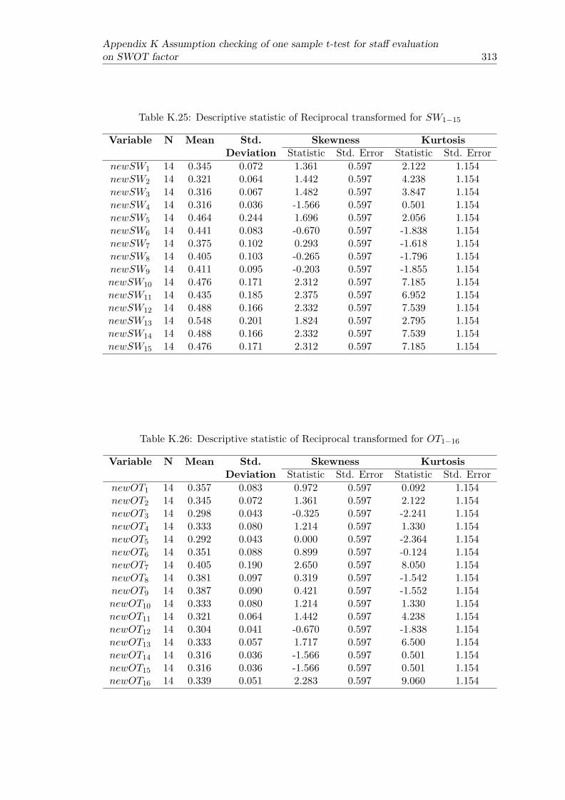
Appendix K Assumption checking of one sample t-test for staff evaluationon SWOT factor 313
Table K.25: Descriptive statistic of Reciprocal transformed for SW1−15
Variable N Mean Std. Skewness KurtosisDeviation Statistic Std. Error Statistic Std. Error
newSW1 14 0.345 0.072 1.361 0.597 2.122 1.154newSW2 14 0.321 0.064 1.442 0.597 4.238 1.154newSW3 14 0.316 0.067 1.482 0.597 3.847 1.154newSW4 14 0.316 0.036 -1.566 0.597 0.501 1.154newSW5 14 0.464 0.244 1.696 0.597 2.056 1.154newSW6 14 0.441 0.083 -0.670 0.597 -1.838 1.154newSW7 14 0.375 0.102 0.293 0.597 -1.618 1.154newSW8 14 0.405 0.103 -0.265 0.597 -1.796 1.154newSW9 14 0.411 0.095 -0.203 0.597 -1.855 1.154newSW10 14 0.476 0.171 2.312 0.597 7.185 1.154newSW11 14 0.435 0.185 2.375 0.597 6.952 1.154newSW12 14 0.488 0.166 2.332 0.597 7.539 1.154newSW13 14 0.548 0.201 1.824 0.597 2.795 1.154newSW14 14 0.488 0.166 2.332 0.597 7.539 1.154newSW15 14 0.476 0.171 2.312 0.597 7.185 1.154
Table K.26: Descriptive statistic of Reciprocal transformed for OT1−16
Variable N Mean Std. Skewness KurtosisDeviation Statistic Std. Error Statistic Std. Error
newOT1 14 0.357 0.083 0.972 0.597 0.092 1.154newOT2 14 0.345 0.072 1.361 0.597 2.122 1.154newOT3 14 0.298 0.043 -0.325 0.597 -2.241 1.154newOT4 14 0.333 0.080 1.214 0.597 1.330 1.154newOT5 14 0.292 0.043 0.000 0.597 -2.364 1.154newOT6 14 0.351 0.088 0.899 0.597 -0.124 1.154newOT7 14 0.405 0.190 2.650 0.597 8.050 1.154newOT8 14 0.381 0.097 0.319 0.597 -1.542 1.154newOT9 14 0.387 0.090 0.421 0.597 -1.552 1.154newOT10 14 0.333 0.080 1.214 0.597 1.330 1.154newOT11 14 0.321 0.064 1.442 0.597 4.238 1.154newOT12 14 0.304 0.041 -0.670 0.597 -1.838 1.154newOT13 14 0.333 0.057 1.717 0.597 6.500 1.154newOT14 14 0.316 0.036 -1.566 0.597 0.501 1.154newOT15 14 0.316 0.036 -1.566 0.597 0.501 1.154newOT16 14 0.339 0.051 2.283 0.597 9.060 1.154


Appendix L
Assumption checking of onesample t-test for staff evaluationon the group of SWOT factor
There are 4 variables represented the average on level of agreement of CPE-KU-KPSstaff towards each aspect of the produced SWOT (denoted as Savg, Wavg, Oavg, Tavg).Before the one-sample t-test will be conducted to test that the average of staff agreementfor each SWOT aspect is not significant from an acceptable threshold, the assumptionsof one sample t-test were checked for each variable in the dataset to ensure that theresult of t-test was valid.
The one-sample t-test required three assumptions to be met as follows (Field, 2009):
Assumption 1: Variables should be interval/ ratio level.
All 4 variables represented the average level of agreement of CPE-KU-KPS staffthat were measured on a scale of 1 to 4. This assumption there was met.
Assumption 2: The data are independent.
Responses to the level of agreement of CPE-KU-KPS staff are independent becausethey come from a different person. This assumption there was met.
Assumption 3: Sampling distribution of the dataset is relatively normal. The nor-mality for each variable was tested by using Shapiro-Wilk in SPSS since the size ofthe dataset is smaller than 2000. A review of the Shapiro-Wilk test for normalityfor variable Savg, Wavg, Oavg and Tavg was shown in Table L.1.
A result of the Shapiro-Wilk test for normality presented in Table L.1 suggeststhat the data is normally distributed since p-values of all variables are greaterthan 0.05.
315

316Appendix L Assumption checking of one sample t-test for staff evaluation
on the group of SWOT factor
Table L.1: Shapiro -Wilk test for normality of variable Savg, Wavg, Oavg andTavg
Variable Shapiro-Wilk NormalityStatistic df p-value
Savg 0.899 7 0.323 YesWavg 0.907 8 0.332 YesOavg 0.951 11 0.658 YesTavg 0.881 5 0.314 Yes
Addition to the normality test, skew and kurtosis of each variable are also observedand shown in Table L.2. Regarding George and Mallery (2003), skew and kurtosisvalues between−1.0 to+1.0 are reasonable ranges to accept that data is reasonablyclose to normal.
Most of the values of skewness and kurtosis reported in Table L.2 were within therange for reasonably concluded that data is relatively normal which is consistentto the result of normality test.
Table L.2: Descriptive statistic of variable Savg, Wavg, Oavg and Tavg
Variable N Mean Std. Skewness KurtosisDeviation Statistic Std. Error Statistic Std. Error
Savg 7 2.929 0.355 -0.731 0.794 -0.905 1.587Wavg 8 2.348 0.224 0.005 0.752 -1.107 1.481Oavg 11 3.188 0.184 0.321 0.661 -0.852 1.279Tavg 5 2.886 0.179 0.828 0.913 -1.217 2.000
In addition to the three assumptions, the significant outliers were investigated througha box plot. In box plots of SPSS, outliers are indicated by a small circle and extremeoutliers are indicated by asterisks (*). Next to these outliers is the number of the caseassociated to the outlier. Figure L.1 shows no sign of extreme outliers for all variables.

Appendix L Assumption checking of one sample t-test for staff evaluationon the group of SWOT factor 317
Figure L.1: Box plots of variables Savg, Wavg, Oavg and Tavg


Appendix M
Experienced users of SWOTsurvey material
M.1 Questionnaire on the quality of an outcome of IPAbased SWOT
This questionnaire forms part of a study into the development of SWOT based oncustomer satisfaction survey. The data collected by this questionnaire is used as a basisfor evaluating the SWOT that has been created. Hence, this survey is very importantfor researchers and to the success of the whole research. Your information will be usedfor this research purpose only. Thank you very much for your time in completing thisquestionnaire.
There are three parts to this questionnaire:
Part I: A case study of creating SWOT
Part II: Questions regarding the quality of produced SWOT
Part III: Demographic questions asking the participant’s background
Please read a case study described in Part I of questionnaire and then indicate the levelof your agreement by ticking X in the provided box in Part II of questionnaire. Finally,please provide some of your information in Part III of questionnaire.
I: A case study of creating SWOTThe department of IT innovation of XYZ University was established in 2006. The mis-sion of the department is to produce graduates with quality, integrity and ethics, aswell as support the country with know-how in the field of information technology. At
319

320 Appendix M Experienced users of SWOT survey material
present, the department of IT innovation still firmly commits to the mission and contin-uously improves teaching quality, research, and academic service to produce specializedgraduates.
With the goal of being in the top 10 in Thailand, the department of IT innovationhas to perform its role effectively. One way to assess how well the performance ofthe department is to conduct student satisfaction survey toward the aspects of thedepartment; for example, Teacher, Computer Facilities etc. This assessment of studentsatisfaction can identify which of department’s aspect meet or not meet the studentsatisfaction. Thus, the department can promote highly performing areas and improvethose poorly performing areas.
To make the best use of data collected through questionnaire, a member of the depart-ment had come up with the idea of using the result of student satisfaction survey toidentify SWOT of the department for formulating a concrete future plan. In order tocreate SWOT based on student satisfaction survey, one section asking students abouttheir level of importance (need/ expectation) with the aspects of the department hadbeen added to the survey. Based on the result of the survey, the strengths and weak-nesses were identified and presented in Table M.1.
Opportunities and threats were identified under a supposition that “the strengths of com-petitor become the threats of the company and the weaknesses of competitors can becomethe opportunities of the company”. Hence, the department of ICT of ABC Universitywas identified as competitor. Then opportunities and threats were identified throughthe survey result of ICT department which collected by using the same questionnaire ofIT innovation department. These opportunities and threats were presented in Table M.1 and steps for generating SWOT were shown in Figure M.1.
Figure M.1: Steps for generating SWOT based on customers satisfaction survey
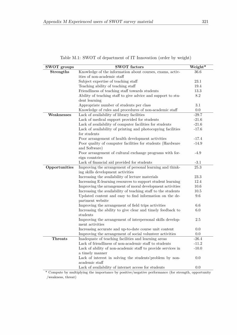
Appendix M Experienced users of SWOT survey material 321
Table M.1: SWOT of department of IT Innovation (order by weight)
SWOT groups SWOT factors Weight*Strengths Knowledge of the information about courses, exams, activ-
ities of non-academic staff36.6
Subject expertise of teaching staff 23.1Teaching ability of teaching staff 19.4Friendliness of teaching staff towards students 13.3Ability of teaching staff to give advice and support to stu-dent learning
8.2
Appropriate number of students per class 3.1Knowledge of rules and procedures of non-academic staff 0.0
Weaknesses Lack of availability of library facilities -29.7Lack of medical support provided for students -21.6Lack of availability of computer facilities for students -21.6Lack of availability of printing and photocopying facilitiesfor students
-17.6
Poor arrangement of health development activities -17.4Poor quality of computer facilities for students (Hardwareand Software)
-14.9
Poor arrangement of cultural exchange programs with for-eign countries
-4.9
Lack of financial aid provided for students -3.1Opportunities Improving the arrangement of personal learning and think-
ing skills development activities25.3
Increasing the availability of lecture materials 23.3Increasing E-learning resources to support student learning 12.4Improving the arrangement of moral development activities 10.6Increasing the availability of teaching staff to the students 10.5Updated content and easy to find information on the de-partment website
9.6
Improving the arrangement of field trips activities 6.6Increasing the ability to give clear and timely feedback tostudents
6.0
Improving the arrangement of interpersonal skills develop-ment activities
2.5
Increasing accurate and up-to-date course unit content 0.0Improving the arrangement of social volunteer activities 0.0
Threats Inadequate of teaching facilities and learning areas -26.4Lack of friendliness of non-academic staff to students -11.2Lack of ability of non-academic staff to provide services ina timely manner
-10.0
Lack of interest in solving the students’problem by non-academic staff
0.0
Lack of availability of internet access for students 0.0* Compute by multiplying the importance by positive/negative performance (for strength, opportunity/weakness, threat)

322 Appendix M Experienced users of SWOT survey material
II: Questions regarding the quality of produced SWOTPlease use SWOT of IT innovation department presented in Table 1 and the step forgenerating SWOT based on customer’s satisfaction survey presented in Figure M.1 toanswer the questions 1-12 by ticking X in the box corresponded to your opinion.
1) Strengths and weakness shown in Table M.1 are explicit (clearly and unambiguouslyformulated).
Strongly disagree Disagree Neither agree Agree Strongly agreenor disagree
� � � � �
2) Opportunities and threats shown in Table M.1 are explicit (clearly and unambiguouslyformulated).
Strongly disagree Disagree Neither agree Agree Strongly agreenor disagree
� � � � �
3) How many SWOT items shown in Table M.1 that is overgeneralised (Too broaddescription)?
All of them Most of them Half of them Some of them None of them(100%) (75%) (50%) (25%) (0%)
� � � � �
4) How many SWOT items shown in Table M.1 that is incorrectly classified as internal/external factors?
All of them Most of them Half of them Some of them None of them(100%) (75%) (50%) (25%) (0%)
� � � � �
5) The SWOT items shown in Table M.1 are comprehensively explain the department’ssituation
Strongly disagree Disagree Neither agree Agree Strongly agreenor disagree
� � � � �
6) All SWOT items shown in Table M.1 are measurable.
Strongly disagree Disagree Neither agree Agree Strongly agreenor disagree
� � � � �

Appendix M Experienced users of SWOT survey material 323
7) The order of SWOT items shown in Table M.1 makes decision-making easier.
Strongly disagree Disagree Neither agree Agree Strongly agreenor disagree
� � � � �
8) The data source for this SWOT analysis is reliable.
Strongly disagree Disagree Neither agree Agree Strongly agreenor disagree
� � � � �
9) The SWOT items shown in Table M.1 can be used as a starting point for strategicplanning.
Strongly disagree Disagree Neither agree Agree Strongly agreenor disagree
� � � � �
10) The SWOT items shown in Table M.1 provide useful information that supportsdecision-making regarding strategic planning.
Strongly disagree Disagree Neither agree Agree Strongly agreenor disagree
� � � � �
11) If you were taken part of developing SWOT for your organisation, how would youlike to use this approach to create SWOT for your company/organisation?
Definitely Probably Neither use Probably Definitelynot use not use nor not use use use
� � � � �
12) What recommendation would you like to make regarding the development of SWOTbased on customer satisfaction?

324 Appendix M Experienced users of SWOT survey material
III: Demographic questions asking the participant’s background
Please tick X in the provided box that corresponds to your answer for each questionbelow:
1. What is your gender? � Male � Prefer not to specify� Female
2. What is your age range? � 21 - 25 � 31 - 35� 26 - 30 � > 35
3. What is your occupation? � Postgraduate student� Business owner� Government Officer� Staff/ Sale Manager� Staff/ Manager of Human Resources� Staff/ Manager of Marketing� Consultant� Other. Please specify
4. Do you have any experience in using SWOT analysis in academia?� No � Yes5. Do you have any practical experience in using SWOT analysisas a basis for strategy development? � No � Yes
If your answer to this question is “Yes”, How many years of practical experiencehave you had in using SWOT analysis? . . . . . .
Thank you very much for your participation in this study.

Appendix M Experienced users of SWOT survey material 325
M.2 Questionnaire on the quality of an outcome of Tradi-tional SWOT
This questionnaire forms part of a study into the development of SWOT based oncustomer satisfaction survey. The data collected by this questionnaire is used as a basisfor evaluating the SWOT that has been created. Hence, this survey is very importantfor researchers and to the success of the whole research. Your information will be usedfor this research purpose only. Thank you very much for your time in completing thisquestionnaire.
There are three parts to this questionnaire:
Part I: A case study of creating SWOT
Part II: Questions regarding the quality of produced SWOT
Part III: Demographic questions asking the participant’s background
Please read a case study described in Part I of questionnaire and then indicate the levelof your agreement by ticking X in the provided box in Part II of questionnaire. Finally,please provide some of your information in Part III of questionnaire.
I: A case study of creating SWOTThe department of IT innovation of XYZ University was established in 2006. The mis-sion of the department is to produce graduates with quality, integrity and ethics, aswell as support the country with know-how in the field of information technology. Atpresent, the department of IT innovation still firmly commits to the mission and contin-uously improves teaching quality, research, and academic service to produce specializedgraduates.
The department of IT innovation arranges an annual meeting in which staff were in-formed and discuss previous and future plans of the department. Staff were also brain-stormed to create SWOT for each aspect of the department such as Teacher, Teaching,Computer Facilities etc. Steps for generating SWOT through brainstorming were shownin Figure M.2 and the produced SWOT factors were presented in Table M.2 - M.5.
The other parts of the questionnaire can be referred to the previous questionnaire shownin Section M.1.
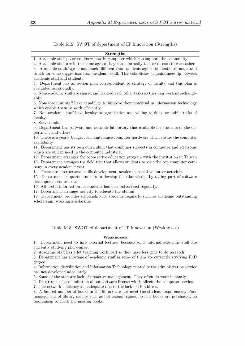
326 Appendix M Experienced users of SWOT survey material
Table M.2: SWOT of department of IT Innovation (Strengths)
Strengths1. Academic staff possesses know-how in computer which can support the community.2. Academic staff are in the same age so they can informally talk or discuss to each other3. Academic staffs’age is not much different from students’age so students are not afraidto ask for some suggestions from academic staff. This establishes acquaintanceship betweenacademic staff and student.4. Department has an action plan correspondent to strategy of faculty and this plan isevaluated occasionally.5. Non-academic staff are shared and learned each other tasks so they can work interchange-ably.6. Non-academic staff have capability to improve their potential in information technologywhich enable them to work efficiently.7. Non-academic staff have loyalty to organisation and willing to do some public tasks offaculty8. Service mind9. Department has software and network laboratory that available for students of the de-partment and others10. There is a yearly budget for maintenance computer hardware which ensure the computeravailability11. Department has its own curriculum that combines subjects in computer and electronicwhich are still in need in the computer industrial12. Department arranges the cooperative education program with the institution in Taiwan13. Department arranges the field trip that allows students to visit the top computer com-pany in every academic year14. There are interpersonal skills development, academic, social volunteer activities15. Department supports students to develop their knowledge by taking part of softwaredevelopment contest etc.16. All useful information for students has been advertised regularly.17. Department arranges activity to educate the alumni18. Department provides scholarship for students regularly such as academic outstandingscholarship, working scholarship
Table M.3: SWOT of department of IT Innovation (Weaknesses)
Weaknesses1. Department need to hire external lecturer because some internal academic staff arecurrently studying phd degree.2. Academic staff has a lot teaching work load so they have less time to do research3. Department has shortage of academic staff as some of them are currently studying PhDdegree.4. Information distribution and Information Technology related to the administration servicehas not developed adequately5. Some of the staff are lack of proactive management. They often do work instantly.6. Department faces limitation about software license which affects the computer service.7. The network efficiency is inadequate due to the lack of IP address.8. A limited number of books in the library are not meet the students’requirement. Poormanagement of library service such as not enough space, no new books are purchased, nomechanism to check the missing books.

Appendix M Experienced users of SWOT survey material 327
Table M.4: SWOT of department of IT Innovation (Opportunities)
Opportunities1. Most of academic staff live in campus which safe their time for travelling to office andenable them to work during night-time. They are also have better working environmentthan staffs working in other University.2. Faculty has granted policy for academic staff with master degree to study PhD degreewithin 2 years since they have started working.3. Students are learned by using the real and updated instrument which allows them to gainexperience and develop their skill continuously.4. Academic staff are subject expertise which is good for knowledge transfer and sharing.5. Students live nearby campus which safe their time for travelling to University and increasean opportunity for learning.6. Department is able to modify the subject in the curriculum in a specific direction as wellas to make it fit with the knowledge and ability of new graduated academic staff.7. Department supports staff to attend a meeting or training for improving their workefficiency.8. By using the curriculum that combines subjects in computer and electronic, studentshave great variety of job opportunities.9. Department has CCNA network laboratory which enables students to learn through thereal network device instead of using the network simulation. This facilitates students toadapt their knowledge in real working situation.10. Field trip in the oversea should be specified in the curriculum so students can visit theoversea company.11. Department should establish the cooperation with local organisation or local industry.12. Department has staff who responsible to advertise information to students via websiteand Facebook which allows students to receive information at a glance.13. There is a clinic in campus in case that student has caught an accident. 14. Departmentsupports student who has problem about tuition fee by allowing them to pay as monthlyinstalments
Table M.5: SWOT of department of IT Innovation (Threats)
Threats1. Compare with other departments that have long been established, the department has nospecific research group or direction as well as has no senior academic staff to be the mentorin doing research.2. Environment and learning area is not encourage students to learn.3. University regulation is less flexible to operate which affects the performance of depart-ment.4. Managing team of the department have a lot teaching load so they have less time to fullymanage the department.5. Special program students are partially received student loan which is not cover the wholeamount of tuition fee.6. The budget for arranging activities of the department is restricted by finance regulationof university.
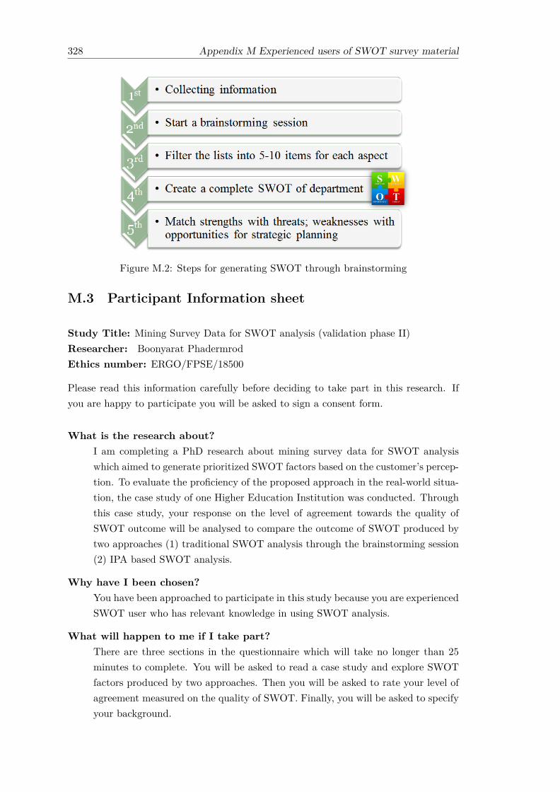
328 Appendix M Experienced users of SWOT survey material
Figure M.2: Steps for generating SWOT through brainstorming
M.3 Participant Information sheet
Study Title: Mining Survey Data for SWOT analysis (validation phase II)Researcher: Boonyarat PhadermrodEthics number: ERGO/FPSE/18500
Please read this information carefully before deciding to take part in this research. Ifyou are happy to participate you will be asked to sign a consent form.
What is the research about?I am completing a PhD research about mining survey data for SWOT analysiswhich aimed to generate prioritized SWOT factors based on the customer’s percep-tion. To evaluate the proficiency of the proposed approach in the real-world situa-tion, the case study of one Higher Education Institution was conducted. Throughthis case study, your response on the level of agreement towards the quality ofSWOT outcome will be analysed to compare the outcome of SWOT produced bytwo approaches (1) traditional SWOT analysis through the brainstorming session(2) IPA based SWOT analysis.
Why have I been chosen?You have been approached to participate in this study because you are experiencedSWOT user who has relevant knowledge in using SWOT analysis.
What will happen to me if I take part?There are three sections in the questionnaire which will take no longer than 25minutes to complete. You will be asked to read a case study and explore SWOTfactors produced by two approaches. Then you will be asked to rate your level ofagreement measured on the quality of SWOT. Finally, you will be asked to specifyyour background.

Appendix M Experienced users of SWOT survey material 329
Are there any benefits in my taking part?By taking part, you have the opportunity to assist the development of a newmethod to generate SWOT based on satisfaction survey which can be used ingovernment, academic institution and private company.
Are there any risks involved?There is no risk involved for participants completing the questionnaire.
Will my participation be confidential?The contents of this questionnaire are absolutely confidential. The name of theparticipants will not be taken and participation will be kept anonymous. All datawill be safe in a protected computer. All will be destroyed once the research iscompleted.
What happens if I change my mind?You have the right to withdraw from doing the questionnaire at any time.
What happens if something goes wrong?If you have any concern or complaint with this research please contacts me (Boon-yarat Phadermrod: [email protected]).
Where can I get more information?If you would like more information on this research please feel free to contact me(Boonyarat Phadermrod: [email protected])
M.4 Result of language consistency translation test of ex-perienced users of SWOT survey
Remark: +1 the question/ instruction is consistent with the English version0 undecided about whether Thai question/ instruction is consistent with the
English version−1 the question/ instruction is not consistent with the English version
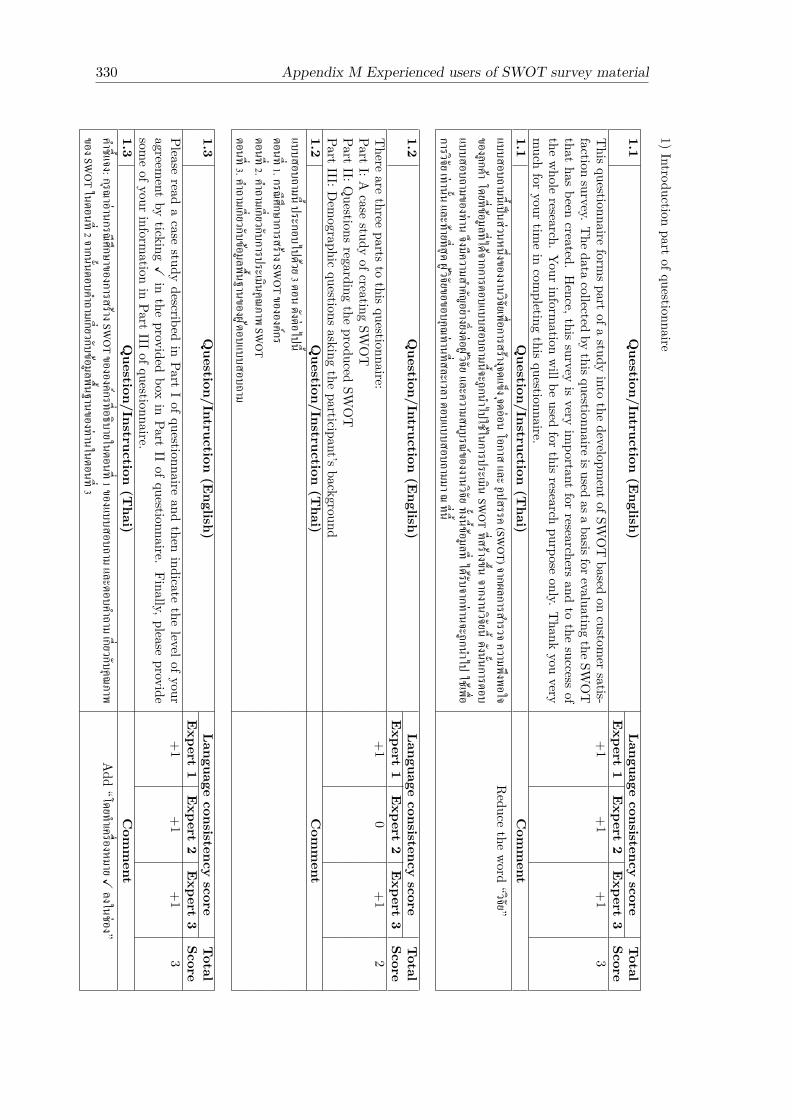
330 Appendix M Experienced users of SWOT survey material
1)Introduction
partofquestionnaire
1.1Question/Intruction
(English)
Languageconsistency
scoreTotal
Expert
1Expert
2Expert
3Score
This
questionnaireform
spartofa
studyinto
thedevelopm
entofSWOT
basedon
customer
satis-faction
survey.The
datacollected
bythisquestionnaire
isusedasa
basisforevaluatingthe
SWOT
thathas
beencreated.
Hence,this
surveyis
veryim
portantfor
researchersand
tothe
successof
thewhole
research.Your
information
willbe
usedfor
thisresearch
purposeonly.
Thank
youvery
much
foryour
timein
completing
thisquestionnaire.
+1
+1
+1
3
1.1Question/Instruction
(Thai)
Com
ment
แบบสอบถามนเปนสวนหนงของงานวจยเพอการสรางจดแขงจดออนโอกาสและอปสรรค(SWOT)จากผลการสารวจความพงพอใจของลกคาโดยทขอมลทไดจากการตอบแบบสอบถามนจะถกนาไปใชในการประเมน
SWOTทสรางขน
จากงานวจยนดงนนการตอบ
แบบสอบถามของทานจงมความสาคญอยางยงตอผวจยและความสมบรณของงานวจยทงนขอมลท
ไดรบจากทานจะถกนาไปใชเพอ
การวจยเทานนและทายทสดผวจยขอขอบคณทานทสละเวลาตอบแบบสอบถามมาณทน
Reduce
theword
“วจย”
1.2Question/Intruction
(English)
Languageconsistency
scoreTotal
Expert
1Expert
2Expert
3Score
There
arethree
partsto
thisquestionnaire:
+1
0+1
2Part
I:Acase
studyofcreating
SWOT
PartII:Q
uestionsregarding
theproduced
SWOT
PartIII:D
emographic
questionsasking
theparticipant’s
background1.2
Question/Instruction
(Thai)
Com
ment
แบบสอบถามนประกอบไปดวย3ตอนดงตอไปนตอนท1.กรณศกษาการสรางSWOTขององคกรตอนท2.คาถามเกยวกบการประเมนคณภาพSWOTตอนท3.คาถามเกยวกบขอมลพนฐานของผตอบแบบสอบถาม
1.3Question/Intruction
(English)
Languageconsistency
scoreTotal
Expert
1Expert
2Expert
3Score
Pleaseread
acase
studydescribed
inPart
Iofquestionnaire
andthen
indicatethe
levelofyouragreem
entby
tickingX
inthe
providedbox
inPart
IIofquestionnaire.
Finally,pleaseprovide
someofyour
information
inPart
IIIofquestionnaire.
+1
+1
+1
3
1.3Question/Instruction
(Thai)
Com
ment
คาชแจง:กรณาอานกรณศกษาของการสรางSWOTขององคกรทอธบายในตอนท1ของแบบสอบถามและตอบคาถามเกยวกบคณภาพของSWOTในตอนท2จากนนตอบคาถามเกยวกบขอมลพนฐานของทานในตอนท3
Add
“โดยทาเครองหมายXลงในชอง”

Appendix M Experienced users of SWOT survey material 331
2)Firstpa
rtof
questio
nnaire
2.1
Que
stion/
Intruc
tion
(Eng
lish)
Lang
uage
consistenc
yscore
Total
Exp
ert1
Exp
ert2
Exp
ert3
Score
Part
I:A
case
stud
yof
creatin
gSW
OT
+1
+1
+1
3The
depa
rtmentof
ITinno
vatio
nof
XYZ
University
wasestablish
edin
2006
.The
miss
ion
ofthede
partmentis
toprod
ucegrad
uateswith
quality
,integrit
yan
dethics,a
swe
llas
supp
ortthe
coun
trywith
know
-how
inthefie
ldof
inform
ationtechno
logy.Atpresent,
thede
partmentof
ITinno
vatio
nstill
firmly
commits
tothem
issionan
dcontinuo
usly
improves
teaching
quality
,research,
andacad
emic
serviceto
prod
ucespecializ
edgrad
uates.
2.1
Que
stion/
Instruction(T
hai)
Com
ment
ตอนท
1.กร
ณศกษ
าการส
รางSW
OTขอ
งองคกร
Add
“อยาง
มงมน
”ภาคว
ชานว
ตกรรมเท
คโนโ
ลยสารส
นเทศ(In
forma
tionT
echnol
ogyInn
ovation)
มหาวท
ยาลยX
YZกอ
ตงขน
ในป
พ.ศ.
2549โ
ดยพน
ธกจข
องภาคว
ชาคอ
ผลตบ
ณฑตท
มความ
รคณ
ธรรม
และจรยธรรม
สรางส
รรคน
วตกร
รมแล
ะถายท
อดเทค
โนโล
ยสสง
คมใน
ปจจบ
นภาควช
านวต
กรรม
เทคโน
โลยส
ารสนเท
ศไดด
าเนนง
านตามพ
นธกจ
ดงกล
าวแล
ะยงคงพ
ฒนาคณภ
าพการเร
ยนการส
อนแล
ะงาน
บรการวชาการอยาง
ตอเนอ
งเพอผ
ลตบณ
ฑตทม
ความเชย
วชาญ
ดานเท
คโนโ
ลยสารส
นเทศ
2.2
Que
stion/
Intruc
tion
(Eng
lish)
Lang
uage
consistenc
yscore
Total
Exp
ert1
Exp
ert2
Exp
ert3
Score
With
thego
alof
beingin
thetop10
inTha
iland
,the
depa
rtmento
fIT
inno
vatio
nha
sto
perfo
rmits
role
effectiv
ely.
One
wayto
assess
how
wellthepe
rform
ance
ofthede
partmentis
tocond
uct
stud
ents
atisfactio
nsurvey
towa
rdtheaspe
ctso
fthe
depa
rtment;fore
xample,
Teache
r,Com
puter
Facilitiesetc.
Thisassessmentof
stud
entsatis
factioncanidentifywhich
ofde
partment’s
aspe
ctmeetor
notmeetthestud
entsatis
faction.
Thu
s,thede
partmentcanprom
otehigh
lype
rform
ing
areasan
dim
provethosepo
orly
perfo
rmingareas.
+1
+1
+1
3
2.2
Que
stion/
Instruction(T
hai)
Com
ment
เพอให
บรรล
เปาหม
ายทจะเปน
ภาคว
ชาเทค
โนโล
ยสารส
นเทศช
นนา1
ใน10
ของป
ระเทศ
ไทยภ
าควช
านวต
กรรม
เทคโน
โลยส
ารสนเท
ศจะตอ
งดาเน
นงาน
อยางม
ประส
ทธภาพ
ซงวธการห
นงใน
การป
ระเมน
ประส
ทธภาพก
ารดาเน
นงาน
ของภาควช
า(Per
forma
nce)ค
อการ
สอบถ
ามคว
ามพง
พอใจข
องนก
ศกษาตอ
ผลการด
าเนนง
านใน
ดานต
างๆขอ
งภาควช
าเชน
อาจาร
ยประจาภ
าควช
าการเร
ยนการส
อนบร
การค
อมพว
เตอรเปน
ตนผล
ประเม
นความ
พงพอ
ใจของนก
ศกษานส
ามารถ
ชใหเห
นวาดาน
ใดขอ
งภาควช
าทนก
ศกษามค
วามพง
พอใจ
กบการด
าเนนง
านแล
ะดาน
ใดขอ
งภาควช
าทมผ
ลการด
าเนนง
านยงไ
มตรงก
บความ
ตองการข
องนก
ศกษา
ซงจะนา
ไปสก
ารปรบ
ปรง
ประส
ทธภาพก
ารดาเน
นงาน
ในสว
นทยงม
ผลการด
าเนนง
านไม
ดเทาทคว
รตลอ
ดจนก
ารพฒน
าประสท
ธภาพ
การด
าเนนง
านขอ
งดาน
ทดอย
แลวใ
หดยงข
น
Rep
lace
“สามารถ
”with
“จะบ
ง”

332 Appendix M Experienced users of SWOT survey material
2)First
partofquestionnaire
(cont)
2.3Question/Intruction
(English)
Languageconsistency
scoreTotal
Expert
1Expert
2Expert
3Score
Tomake
thebest
useofdata
collectedthrough
questionnaire,amem
berofthe
department
hadcom
eup
with
theidea
ofusing
theresult
ofstudent
satisfactionsurvey
toidentify
SWOT
ofthe
department
forform
ulatingaconcrete
futureplan.
Inorder
tocreate
SWOT
baseon
studentsatisfaction
survey,onesection
askingstudentsabouttheirlevelofim
portance(need/
expectation)with
theaspectsofthedepartmenthad
beenadded
tothesurvey.Based
ontheresultofthesurvey,
thestrengths
andweaknesses
wereidentified
andpresented
inTable
1.
+1
+1
+1
3
2.3Question/Instruction
(Thai)
Com
ment
นอกจากนหนงในสมาชกของภาควชาไดเสนอแนวคดการวเคราะหSWOTของภาควชาจากผลการประเมนความพงพอใจของนกศกษาอกดวยโดยSWOT
ทไดจะถกใชเปนขอมลสาหรบการสรางแผนพฒนาภาควชาในอนาคตทงนสวนคาถามเกยวกบความคดเหนของ
นกศกษาตอระดบความสาคญ(Importance)ในดานตางๆของภาควชาไดถกเพมเตมลงในแบบประเมนความพงพอใจของนกศกษาเพอประเมนวาดานตางๆของภาควชาสงผลตอคณภาพการศกษาของนกศกษามากหรอนอยเพยงใดหลงจากทภาควชาไดทาการสารวจความพงพอใจของนกศกษาโดยใชแบบประเมนทไดออกแบบมานน
จดแขงและจดออนของภาควชานวตกรรมเทคโนโลยสารสนเทศจงถกสรางขนจากผลการประเมนความพงพอใจของนกศกษาดงแสดงในตารางท1.
2.4Question/Intruction
(English)
Languageconsistency
scoreTotal
Expert
1Expert
2Expert
3Score
Opportunities
andthreats
wereidentified
underasupposition
that“the
strengthsofcom
petitorbecom
ethethreatsofthecompany
andtheweaknessesofcom
petitorscanbecom
etheopportunitiesofthe
company”.
Hence,the
department
ofICT
ofABC
University
wasidentified
ascom
petitor.Then
opportunitiesandthreatswere
identifiedthrough
thesurvey
resultofICT
departmentw
hichcollected
byusing
thesam
equestionnaire
ofITinnovation
department.
These
opportunitiesand
threatswere
presentedin
Table1and
stepsfor
generatingSW
OT
wereshow
nin
Figure1.
+1
+1
+1
3
2.4Question/Instruction
(Thai)
Com
ment
โอกาสและอปสรรค
ถกสรางขนตามสมมตฐานทวา“จดแขงของคแขงขององคกรถอเปน
อปสรรคขององคกรและจดออนของ
คแขงขององคกรถอเปนโอกาสขององคกร”ในกรณศกษาน
ภาควชาเทคโนโลยสารสนเทศและการสอสาร(InformationandCom-munication
Technology,ICT)มหาวทยาลยABC
ถกเลอกใหเปนคแขงของภาควชานวตกรรมเทคโนโลยสารสนเทศดงนนโอกาส
และอปสรรคของภาควชานวตกรรมเทคโนโลยสารสนเทศ
จงถกสรางขนจากผลการประเมนความพงพอใจของนกศกษาICTทเกบ
ขอมลโดยใชแบบสอบถามชดเดยวกนกบทภาควชานวตกรรมเทคโนโลยสารสนเทศใชโอกาสและ
อปสรรคของภาควชานวตกรรมเทคโนโลยสารสนเทศทถกสรางขนนนแสดงในตารางท1และขนตอนการสรางSWOTจากแบบประเมนความพงพอใจของลกคานนแสดงในรปท1.

Appendix M Experienced users of SWOT survey material 333
2)Se
cond
part
ofqu
estio
nnaire
Que
stion/
Instruction
Que
stion/
Instruction
Lang
uage
consistenc
yscore
Total
Com
ment
(Eng
lish)
(Tha
i)Ex
pert
Expe
rtEx
pert
Score
12
33.
1II:Que
stions
rega
rding
theprod
uced
SWOT
ตอนท
2.คาถามเก
ยวกบ
การป
ระเมน
คณภาพS
WOT
+1
0+1
2
Please
useSW
OT
ofIT
inno
vatio
nde
-pa
rtmentpresentedin
Table1an
dthe
step
forgene
ratin
gSW
OT
based
oncu
stom
ers’s
atisfactio
nsurvey
presented
inFigu
re1to
answ
ertheq
uestions
1-12
bytic
king
Xin
theb
oxcorrespo
nded
toyo
urop
inion.
คาชแ
จง:จาก
SWOT
ของกรณ
ศกษาขอ
งภาควช
านว
ตกรรมเท
คโนโ
ลยสารส
นเทศ
แสดงใน
ตาราง
ท1
และข
นตอน
การส
รางSW
OTแส
ดงใน
รปท1ก
รณา
ตอบ
คาถามข
อ1-1
2โดย
ทาเคร
องหม
ายถก(X
)ใน
ชองท
ตรงกบค
วามคด
เหนขอ
งทาน
มากท
สด
Add
“จากแบ
บประเมน
ความพง
พอใจข
องลก
คา”
3.2
Streng
thsa
ndwe
akne
ssshow
nin
Table
1areexplicit
(clearly
and
unam
bigu
-ou
slyform
ulated
).
จดแข
งและ
จดออ
นแสด
งในตาราง
ท1มค
วามชด
เจนเขา
ใจงาย
ไมกากว
ม+1
+1
+1
3
3.3
Opp
ortunitie
sand
threatss
hownin
Ta-
ble1
areexplicit
(clearly
and
unam
-bigu
ously
form
ulated
).
โอกาส
และ
อปสร
รคแส
ดงใน
ตาราง
ท1
มความ
ชดเจน
เขาใจง
ายไม
กากว
ม+1
+1
+1
3
3.4
How
man
ySW
OT
itemsshow
nin
Ta-
ble1that
isovergene
ralised
(Too
broa
dde
scrip
tion)?
จากตาราง
ท1ม
จานวน
รายการS
WOTกร
ายการท
มคว
ามหม
ายกวาง
เกนไป
ไมเฉพ
าะเจาะ
จง+1
+1
+1
3
3.5
How
man
ySW
OTite
mss
hownin
Table
1that
isincorrectly
classifi
edas
inter-
nal/external
factors?
จากตาราง
ท1มจ
านวน
รายการS
WOTก
รายการท
ถกจด
กลมเป
นปจจยภ
ายใน/ภ
ายนอก
ทไมถ
กตอง
+1
+1
+1
3
3.6
The
SWOT
itemsshow
nin
Table
1arec
ompreh
ensiv
elyexplainthed
epart-
ment’s
situa
tion
รายการ
SWOT
แสดงใน
ตาราง
ท1
สามารถ
อธบาย
สถาน
การณ
ขององคกร
ไดคร
อบคล
มรอบ
ดาน
+1
+1
+1
3
3.7
AllSW
OT
itemsshow
nin
Table1are
measurable.
รายการS
WOTแส
ดงใน
ตาราง
ท1ส
ามารถ
วดแล
ะเปร
ยบเทย
บได
+1
+1
+1
3Add
“ทงห
มด”
3.8
The
orde
rofS
WOTite
mss
hownin
Ta-
ble1mak
esde
cisio
n-mak
ingeasie
r.การเร
ยงลาดบข
องราย
การS
WOTแส
ดงใน
ตาราง
ท1
ทาให
การต
ดสนใ
จเกยวกบ
แผนข
ององคก
รงายข
น+1
+1
+1
3Rep
lace
“ทา”
with
“ชวย”
3.9
The
data
source
fort
hisS
WOTan
alysis
isrelia
ble.
แหลงขอ
มลสาหร
บวเคร
าะหSW
OTแส
ดงใน
ตาราง
ท1ม
ความนา
เชอถอ
+1
+1
+1
3Rep
lace
“สาห
รบ”with
“ทนา
มาใชเพอ
การ”

334 Appendix M Experienced users of SWOT survey material
2)Second
partofquestionnaire
(cont)
Question/
InstructionQuestion/
InstructionLanguage
consistencyscore
TotalCom
ment
(English)(T
hai)Expert
ExpertExpert
Score1
23
3.10The
SWOT
itemsshow
nin
Table1can
beused
asastarting
pointforstrategicplanning.
รายการSWOTแสดงในตารางท
1สามารถนาไปใชสาหรบการวางแผนกลยทธขององคกรได
+1
+1
+1
3
3.11The
SWOT
itemsshow
nin
Table1
provideuseful
information
thatsup-
portsdecision-making
regardingstrate-
gicplanning.
รายการSWOT
แสดงในตารางท1
นามาซงขอมลท
เปนประโยชนตอการตดสนใจเกยวกบแผนขององคกร
+1
+1
+1
3Replace
“เกยวกบแผน”with
“วางแผนกลยทธ”
3.12If
youwere
takenpart
ofdevelop-
ingSW
OT
foryour
organisation,how
wouldyou
liketo
usethis
approachto
createSW
OT
foryour
company
/organisation?
หากทานมบทบาทในการสรางSWOTในองคกรของ
ทานทานจะนาวธการสราง
SWOTแสดงในรปท
1ไปใชในการสรางSWOT
ของบรษทหรอองคกรของทานหรอไม
+1
-1+1
1Check
theuse
ofHow
andYes/N
oquestion
3.13W
hatrecom
mendation
wouldyou
liketo
make
regardingthe
development
ofSW
OT
basedon
customersatisfaction?
ขอเสนอแนะของทานตอการสรางSWOT
จากผลสารวจความพงพอใจของลกคา
+1
-1+1
1Change
Thai
sen-tence
tobe
thequestion
3.14Strongly
disagreeไมเหนดวยอยางยง
+1
+1
+1
3Disagree
ไมเหนดวยNeither
agreenor
disagreeไมใชทงเหนดวยหรอไมเหนดวย
Agree
เหนดวยStrongly
agreeเหนดวยอยางยง
3.15Allofthem
(100%)
ทงหมดของรายการ(100%)+1
+1
+1
3Replace
“ทงหมด”Most
ofthem(75%
)สวนใหญของรายการ(75%)
with
“ทก”Halfofthem
(50%)
ครงหนงของรายการ(50%)Som
eofthem
(25%)
บางสวนของรายการ(25%)None
ofthem(0%
)ไมม(0%)
3.16Definitely
notuse
ไมนาไปใชอยางแนนอน+1
+1
+1
3Probably
notuse
อาจจะไมนาไปใชNeither
usenor
notuse
ไมแนใจProbably
useอาจจะนาไปใช
Definitely
useนาไปใชอยางแนนอน

Appendix M Experienced users of SWOT survey material 335
3)Third
part
ofqu
estio
nnaire
Que
stion/
Instruction
Que
stion/
Instruction
Lang
uage
consistenc
yscore
Total
Com
ment
(Eng
lish)
(Tha
i)Ex
pert
Expe
rtEx
pert
Score
12
34.1
III:
Dem
ograph
icqu
estio
nsasking
the
participan
t’sba
ckgrou
ndตอ
นท3.
คาถามเก
ยวกบ
ขอมล
พนฐาน
ของผต
อบแบ
บสอบ
ถาม
+1
+1
+1
3
Please
tickX
intheprov
ided
boxthat
correspo
ndsto
your
answ
erforeach
questio
nbe
low:
คาชแ
จง:กร
ณาทาเคร
องหม
ายถก(
X)ใ
นชองทต
รงกบ
ขอมล
ของท
านมากท
สด
4.2
Wha
tis
your
gend
er?
เพศ+1
+1
+1
3�
Male�
Female
�ชาย�
หญง
�Pr
efer
notto
specify
�ไม
ตองการร
ะบ4.3
Wha
tis
your
agerang
e?อาย
+1
+1
+1
3Su
ggest
touse
“ชวง
อาย”
4.4
Wha
tis
your
occu
patio
n?อาชพ
+1
+1
-11
Che
ckaprop
erwo
rd�
Stud
ents
�นก
ศกษา
ระดบ
บณฑต
ศกษา
ofoccu
patio
nlist
�Bu
sinessow
ners
�เจา
ของธรก
จสวน
ตว�
Governm
entOfficers
�พน
กงาน
ของรฐ
/ขาราช
การ
�Marketin
g/Sa
lesMan
agers
�พน
กงาน
การต
ลาด/ผ
จดการฝายข
าย�
Person
nel/Hum
anResou
rces
Man
-ag
ers
�พน
กงาน
ฝายบค
คล/ผจด
การฝายบ
คคล
�Con
sulta
nts
�ทป
รกษา
�Other.Please
specify
�อน
ๆโปร
ดระบ
4.5
Do
you
have
any
expe
rienc
ein
using
SWOT
analysis
inacad
emia?
ทานเค
ยเรยน
เกยวก
บการว
เคราะห
SWOT
ในสถ
าบน
ศกษาหร
อไม?
00
-1-1
Add
“หรอมป
ระสบ
การณ
”
�Ye
s�
No
�เคย
�ไม
เคย4.6
Doyo
uha
vean
ypractic
alexpe
rienc
ein
usingSW
OT
analysis
asaba
sisfor
strategy
developm
ent?
ทานม
ประส
บการณ
การวเคร
าะหSW
OTเพอ
สราง
แผนก
ลยทธ
ในองคก
รหรอหน
วยงาน
ของท
านหร
อไม
0+1
01
Che
ckthe
consis-
tenc
yof
theop
tionof
questio
n4.5an
d4.6
�Ye
s�
No
�ม
�ไม
มIfyo
uran
swer
tothisqu
estio
nis“Y
es”,
How
man
yyearso
fpractical
expe
rienc
eha
veyo
uha
din
usingSW
OT
analysis?
กรณา
ระบจ
านวน
ปททานม
ประส
บการณ
การวเคร
าะหSW
OT


Appendix N
Assumption checking of twoindependent sample t-teston experienced users of SWOTevaluation
There are 10 variables represented the rating score of MBA students towards each ques-tion related to the quality of SWOT (denoted as q1− q10). Before performing the t-test,assumptions of t-test must be met for the test to be accurate. The two independent sam-ple t-test assumes that sample data are measured at least at the interval level, sampledata is normally distributed, the variances of the two groups are equal (Homogeneity ofvariance) and the two groups of samples are independent from each other (Field, 2009).Detail regarding the assumptions checking is explained below:
Assumption 1: Variables should be interval/ ratio level.
All 10 variables represented the rating score of MBA students that were measuredon a scale of 1 to 5. This assumption there was met.
Assumption 2: The data are independent.
Responses to the quality of SWOT of MBA students are independent becausethey come from different participants. There were also different participants ineach group with no participant being in more than one group. This assumptionthere was met.
Assumption 3: Sampling distribution of the dataset is relatively normal. The nor-mality for each variable within each group was tested by using Shapiro-Wilk inSPSS since the size of the dataset is smaller than 2000. A review of the Shapiro-Wilk test for normality for variable q1 − q10 is shown in Table N.1.
337
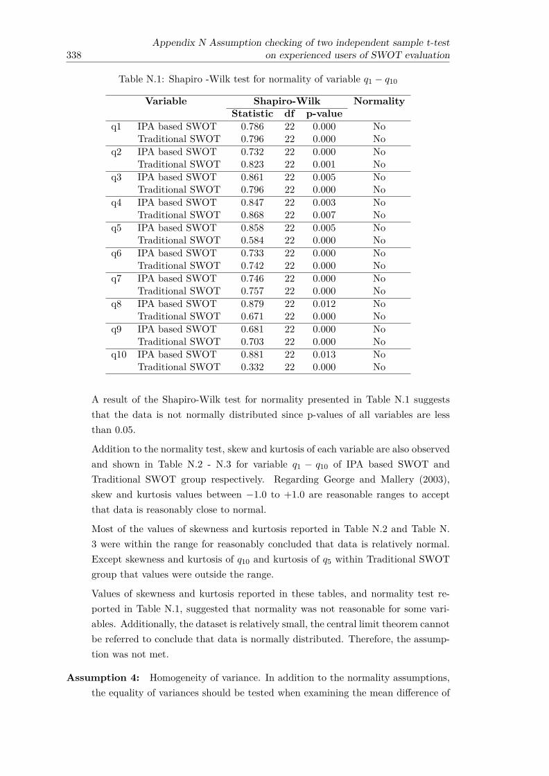
338Appendix N Assumption checking of two independent sample t-test
on experienced users of SWOT evaluation
Table N.1: Shapiro -Wilk test for normality of variable q1 − q10
Variable Shapiro-Wilk NormalityStatistic df p-value
q1 IPA based SWOT 0.786 22 0.000 NoTraditional SWOT 0.796 22 0.000 No
q2 IPA based SWOT 0.732 22 0.000 NoTraditional SWOT 0.823 22 0.001 No
q3 IPA based SWOT 0.861 22 0.005 NoTraditional SWOT 0.796 22 0.000 No
q4 IPA based SWOT 0.847 22 0.003 NoTraditional SWOT 0.868 22 0.007 No
q5 IPA based SWOT 0.858 22 0.005 NoTraditional SWOT 0.584 22 0.000 No
q6 IPA based SWOT 0.733 22 0.000 NoTraditional SWOT 0.742 22 0.000 No
q7 IPA based SWOT 0.746 22 0.000 NoTraditional SWOT 0.757 22 0.000 No
q8 IPA based SWOT 0.879 22 0.012 NoTraditional SWOT 0.671 22 0.000 No
q9 IPA based SWOT 0.681 22 0.000 NoTraditional SWOT 0.703 22 0.000 No
q10 IPA based SWOT 0.881 22 0.013 NoTraditional SWOT 0.332 22 0.000 No
A result of the Shapiro-Wilk test for normality presented in Table N.1 suggeststhat the data is not normally distributed since p-values of all variables are lessthan 0.05.
Addition to the normality test, skew and kurtosis of each variable are also observedand shown in Table N.2 - N.3 for variable q1 − q10 of IPA based SWOT andTraditional SWOT group respectively. Regarding George and Mallery (2003),skew and kurtosis values between −1.0 to +1.0 are reasonable ranges to acceptthat data is reasonably close to normal.
Most of the values of skewness and kurtosis reported in Table N.2 and Table N.3 were within the range for reasonably concluded that data is relatively normal.Except skewness and kurtosis of q10 and kurtosis of q5 within Traditional SWOTgroup that values were outside the range.
Values of skewness and kurtosis reported in these tables, and normality test re-ported in Table N.1, suggested that normality was not reasonable for some vari-ables. Additionally, the dataset is relatively small, the central limit theorem cannotbe referred to conclude that data is normally distributed. Therefore, the assump-tion was not met.
Assumption 4: Homogeneity of variance. In addition to the normality assumptions,the equality of variances should be tested when examining the mean difference of

Appendix N Assumption checking of two independent sample t-teston experienced users of SWOT evaluation 339
Table N.2: Descriptive statistic of variable q1 − q10 (IPA based SWOT group)
Variable N Mean Std. Skewness KurtosisDeviation Statistic Std. Error Statistic Std. Error
q1 22 3.364 0.790 -0.781 0.491 3.030 0.953q2 22 3.318 0.568 -0.050 0.491 -0.506 0.953q3 22 3.364 0.790 -0.142 0.491 -0.352 0.953q4 22 3.000 0.926 0.396 0.491 -0.892 0.953q5 22 3.364 0.902 -0.835 0.491 1.025 0.953q6 22 3.864 0.560 -0.074 0.491 0.459 0.953q7 22 4.045 0.576 0.014 0.491 0.510 0.953q8 22 3.409 1.008 -0.034 0.491 -1.016 0.953q9 22 3.500 0.740 -1.163 0.491 -0.019 0.953q10 22 3.409 0.854 0.058 0.491 -0.399 0.953
Table N.3: Descriptive statistic of variable q1 − q10 (Traditional SWOT group)
Variable N Mean Std. Skewness KurtosisDeviation Statistic Std. Error Statistic Std. Error
q1 22 3.227 0.752 -0.413 0.491 -1.036 0.953q2 22 3.500 0.673 0.000 0.491 0.043 0.953q3 22 3.227 0.752 -0.413 0.491 -1.036 0.953q4 22 3.136 0.834 0.269 0.491 -0.363 0.953q5 22 3.909 0.426 -0.637 0.491 3.168 0.953q6 22 3.409 0.734 -0.847 0.491 -0.538 0.953q7 22 3.273 0.827 -0.574 0.491 -1.282 0.953q8 22 4.182 0.501 0.413 0.491 0.752 0.953q9 22 4.091 0.526 0.142 0.491 1.116 0.953q10 22 4.091 0.294 3.059 0.491 8.085 0.953
two independent samples in order to guarantee that the difference between groupsis not affected by variance. This assumption can be tested with Levene’s test(Field, 2009).
Levene’s test checks whether the variances of sample groups are statistically dif-ferent. The Levene’s test hypotheses are:
H0: variances are the sameH1: variances are different
For each question, Levene’s test was conducted to test the equality of variance oftwo groups and the result of Levene’s test is shown in Table N.4.
Referring to Table N.4, for the rating on variable q1− q4, the variances were equalfor IPA based SWOT and Traditional SWOT group since p-value of these variableswere higher than 0.05. But for variable q5 − q10 the variances were significantlydifferent in the two groups since p-value of these variables were less than 0.05.The assumption of homogeneity of variance there was not consistently met for allvariables.
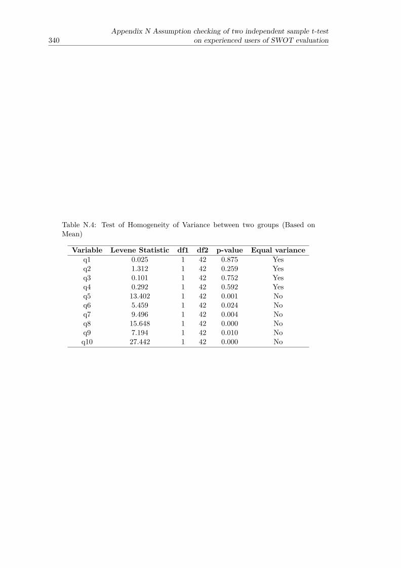
340Appendix N Assumption checking of two independent sample t-test
on experienced users of SWOT evaluation
Table N.4: Test of Homogeneity of Variance between two groups (Based onMean)
Variable Levene Statistic df1 df2 p-value Equal varianceq1 0.025 1 42 0.875 Yesq2 1.312 1 42 0.259 Yesq3 0.101 1 42 0.752 Yesq4 0.292 1 42 0.592 Yesq5 13.402 1 42 0.001 Noq6 5.459 1 42 0.024 Noq7 9.496 1 42 0.004 Noq8 15.648 1 42 0.000 Noq9 7.194 1 42 0.010 Noq10 27.442 1 42 0.000 No

References
Akiyoshi, M. and Komoda, N. (2005). An analysis framework of enterprise documentsfor business strategy design. In International Conference on Intelligent Agents, WebTechnologies and Internet Commerce, volume 1, pages 65–69. IEEE.
Allen, D. R. and Wilburn, M. (2002). Why customer satisfaction. In Linking customerand employee satisfaction to the bottom line, pages 1–16. ASQ Quality Press.
Avison, D. and Elliot, S. (2006). Scoping the discipline of information systems. In Infor-mation Systems: The State of the Field, pages 3–18. John Wiley & Sons Chichester,UK.
Ayub, A., Razzaq, A., Aslam, M. S., and Iftekhar, H. (2013). A conceptual frameworkon evaluating swot analysis as the mediator in strategic marketing planning throughmarketing intelligence. European Journal of Business and Social Sciences, 2(1):91–98.
Azzalini, A., Scarpa, B., and Walton, G. (2012). Data analysis and data mining: anintroduction. Oxford University Press.
Azzopardi, E. and Nash, R. (2013). A critical evaluation of importance-performanceanalysis. Tourism Management, 35:222–233.
Bacon, D. R. (2003). A comparison of approaches to importance-performance analysis.International Journal of Market Research, 45(1):55–72.
Ban, O.-I. and Bogdan, V. (2013). Using partial correlation coefficient to assess theimportance of quality attributes: Study case for tourism romanian consumers. Eco-nomics, Business and Management, 1(1):21–24.
Bansback, N., Li, L. C., Lynd, L., and Bryan, S. (2014). Exploiting order effects toimprove the quality of decisions. Patient education and counseling, 96(2):197–203.
Ben-Gal, I. (2007). Bayesian networks. In Encyclopedia of statistics in quality andreliability. Wiley Online Library.
Bender, R. and Benner, A. (2000). Calculating ordinal regression models in SAS andS-Plus. Biometrical Journal, 42(6):677–699.
341
342 REFERENCES
Blair, J., Czaja, R. F., and Blair, E. A. (2013). Data collection I: Selecting a method.In Designing Surveys: A Guide to Decisions and Procedures: A Guide to Decisionsand Procedures, pages 48–82. Sage Publications.
Bosnjak, M. (2014). Customer satisfaction. In Encyclopedia of quality of life and well-being research, pages 1409–1412. Springer Science+Business Media Dordrech.
Cassel, C. (2006). Measuring customer satisfaction, a methodological guidance. StatisticsSweden, 2(2).
Cengiz, E. (2010). Measuring customer satisfaction: Must or not? Journal of NavalScience and Engineering, 6(2):76–88.
Chang, H.-H. and Huang, W.-C. (2006). Application of a quantification SWOT analyt-ical method. Mathematical and Computer Modelling, 43(1):158–169.
Chen, C.-K. and Hughes, J. (2004). Using ordinal regression model to analyze studentsatisfaction questionnaires. IR applications, 1(1):1–12.
Chen, L.-F., Lin, S.-P., and Lin, Y.-C. (2010). Application of IPA and Back-PropagationNeural Network to build a new service quality decision making model. InternationalJournal of Information and Management Sciences, 21:31.
Chen, P. Y. and Popovich, P. M. (2002). The pearson product-moment correlation. InCorrelation: Parametric and nonparametric measures, pages 9–24. Sage Publications.
Cheng, J. and Greiner, R. (2001). Learning bayesian belief network classifiers: Algo-rithms and system. In Advances in Artificial Intelligence, pages 141–151. Springer.
Chrzan, K. and Golovashkina, N. (2006). An empirical test of six stated importancemeasures. International Journal of Market Research, 48(6):717–740.
Chu, R. (2002). Stated-importance versus derived-importance customer satisfactionmeasurement. Journal of Services Marketing, 16(4):285–301.
Cohen, S. (2003). Maximum difference scaling: Improved measures of importance andpreference for segmentation. In Sawtooth Software Conference Proceedings, SawtoothSoftware, Inc, volume 530, pages 61–74.
Coman, A. and Ronen, B. (2009). Focused SWOT: diagnosing critical strengths andweaknesses. International Journal of Production Research, 47(20):5677–5689.
Cover, T. M. and Thomas, J. A. (2006). Entropy, relative entropy, and mutual infor-mation. In Elements of information theory, pages 13–54. Wiley-interscience.
Cugnata, F. and Salini, S. (2013). Model-based approach for importance–performanceanalysis. Quality & Quantity, pages 1–12.

REFERENCES 343
Dai, Y., Kakkonen, T., and Sutinen, E. (2011). MinEDec: a decision-support model thatcombines text-mining technologies with two competitive intelligence analysis methods.International Journal of Computer Information Systems and Industrial ManagementApplications, 3:165–173.
Datamonitor (2003). eBay Inc. SWOT Analysis. http://www.advisorgate.com/files/p10.pdf Accessed (April 27, 2013).
De Vaus, D. (2002a). Administering questionnaires. In Surveys in social research, pages122–144. Allen & Unwin.
De Vaus, D. (2002b). Building scales. In Surveys in social research, pages 180–199.Allen & Unwin.
Dejaeger, K., Goethals, F., Giangreco, A., Mola, L., and Baesens, B. (2012). Gaining in-sight into student satisfaction using comprehensible data mining techniques. EuropeanJournal of Operational Research, 218(2):548–562.
Deng, W.-J., Chen, W.-C., and Pei, W. (2008a). Back-propagation neural network basedimportance–performance analysis for determining critical service attributes. ExpertSystems with Applications, 34(2):1115–1125.
Deng, W.-J., Kuo, Y.-F., and Chen, W.-C. (2008b). Revised importance–performanceanalysis: three-factor theory and benchmarking. The Service Industries Journal,28(1):37–51.
Domingos, P. and Pazzani, M. (1997). On the optimality of the simple bayesian classifierunder zero-one loss. Machine learning, 29(2-3):103–130.
Doyle, J. R., Green, R. H., and Bottomley, P. A. (1997). Judging relative importance:direct rating and point allocation are not equivalent. Organizational behavior andhuman decision processes, 70(1):65–72.
du Toit, A. (2016). Using environmental scanning to collect strategic information: ASouth African survey. International Journal of Information Management, 36(1):16–24.
Duan, L. and Da Xu, L. (2012). Business intelligence for enterprise systems: a survey.IEEE Transactions on Industrial Informatics, 8(3):679–687.
Duke, C. R. and Mount, A. S. (1996). Rediscovering performance-importance analysisof products. Journal of Product & Brand Management, 5(2):43–54.
Dyson, R. G. (2004). Strategic development and SWOT analysis at the University ofWarwick. European journal of operational research, 152(3):631–640.
344 REFERENCES
Easterbrook, S., Singer, J., Storey, M.-A., and Damian, D. (2008). Selecting empiricalmethods for software engineering research. In Guide to advanced empirical softwareengineering, pages 285–311. Springer.
Eskildsen, J. K. and Kristensen, K. (2006). Enhancing importance-performance analysis.International Journal of Productivity and Performance Management, 55(1):40–60.
Fayyad, U., Piatetsky-Shapiro, G., and Smyth, P. (1996a). From data mining to knowl-edge discovery in databases. AI magazine, 17(3):37.
Fayyad, U., Piatetsky-Shapiro, G., Smyth, P., et al. (1996b). Knowledge discovery anddata mining: Towards a unifying framework. Knowledge Discovery and Data Mining,pages 82–88.
Fehringer, D., Hohhof, B., and Johnson, T. (2006). State of the art: competitive intel-ligence. Competitive Intelligence Foundation, Washington.
Feng, M., Mangan, J., Wong, C., Xu, M., and Lalwani, C. (2014). Investigating the dif-ferent approaches to importance–performance analysis. The Service Industries Jour-nal, 34(12):1021–1041.
Field, A. (2009). Discovering statistics using SPSS. Sage publications.
Figini, S. and Giudici, P. (2007). Statistical models for customer satisfaction data.Journal of Quality Technology and Quality Management, 7(1):69–82.
Fincham, J. E. (2008). Response rates and responsiveness for surveys, standards, andthe journal. American journal of pharmaceutical education, 72(2):43.
Fink, A. (2003). How to ask survey questions, volume 4. Sage Publications.
Fink, A. (2012a). Conducting surveys: Everyone is doing it. In How to Conduct Surveys:A Step-by-Step Guide: A Step-by-Step Guide, pages 1–28. Sage Publications.
Fink, A. (2012b). The survey form: questions, scales, and appearance. In How toConduct Surveys: A Step-by-Step Guide: A Step-by-Step Guide, pages 29–56. SagePublications.
Fontenot, G., Henke, L., Carson, K., and Carson, P. P. (2007). Techniques for determin-ing importance: balancing scientific method and subjectivity. Journal of Targeting,Measurement and Analysis for Marketing, 15(3):170–180.
Ford, J. B., Joseph, M., and Joseph, B. (1999). Importance-performance analysis as astrategic tool for service marketers: the case of service quality perceptions of businessstudents in new zealand and the usa. Journal of Services Marketing, 13(2):171–186.
Fornell, C., Johnson, M. D., Anderson, E. W., Cha, J., and Bryant, B. E. (1996). Theamerican customer satisfaction index: nature, purpose, and findings. the Journal ofMarketing, pages 7–18.
REFERENCES 345
Fouladgar, M. M., Yakhchali, S. H., Yazdani-Chamzini, A., and Basiri, M. H. (2011).Evaluating the strategies of Iranian mining sector using a integrated model. In 2011 In-ternational Conference on Financial Management and Economics Proceedings, pages58–63.
Free Management E-books, . (2013). Pestle analysis: Strategy skills. www.free-management-ebooks.com/dldebk/dlst-pestle.htm Accessed (June 18, 2016).
Friedman, N., Geiger, D., and Goldszmidt, M. (1997). Bayesian network classifiers.Machine learning, 29(2-3):131–163.
Fritz, C. O., Morris, P. E., and Richler, J. J. (2012). Effect size estimates: currentuse, calculations, and interpretation. Journal of Experimental Psychology: General,141(1):2.
Fullerton, A. S. (2009). A conceptual framework for ordered logistic regression models.Sociological methods & research, 38(2):306–347.
Gao, C.-Y. and Peng, D.-H. (2011). Consolidating SWOT analysis with nonhomogeneousuncertain preference information. Knowledge-Based Systems, 24(6):796–808.
Garland, R. (1991). The mid-point on a rating scale: Is it desirable. Marketing bulletin,2(1):66–70.
Garson, G. D. (1991). Interpreting neural-network connection weights. AI Expert, 6(4):46–51.
Garver, M. S. (2003). Best practices in identifying customer-driven improvement oppor-tunities. Industrial Marketing Management, 32(6):455–466.
George, D. and Mallery, M. (2003). SPSS for windows step by step: A simple studyguide and reference, 11.0 update. Allyn and Bacon Boston.
Ghazinoory, S., Abdi, M., and Azadegan-Mehr, M. (2011). SWOT Methodology: AState-of-the-Art Review for the Past, A Framework for the Future. Journal of BusinessEconomics and Management, 12(1):24–48.
Glasow, P. A. (2005). Fundamentals of survey research methodology. MITRE Wash-ington C3 Centre, 18(April):1–12.
Global Markets Direct (2012). Amazon . com , Inc . - Financial and Strategic AnalysisReview. http://callisto.ggsrv.com Accessed (April 27, 2013).
Glorfeld, L. W. (1996). A methodology for simplification and interpretation ofbackpropagation-based neural network models. Expert Systems with Applications,10(1):37–54.
Goff, B. A., Schack, R. W., and Veth, J. (2002). Customer Satisfaction Handbook.Technical report, Charter Oak Group.

346 REFERENCES
Gonçalves, J. R., Pinto, A., Batista, M. J., Pereira, A. C., and BoviAmbrosano, G. M.(2014). Importance-performance analysis: Revisiting a tool for the evaluation ofclinical services. Health (1949-4998), 6(5).
Gorener, A. (2012). Comparing ahp and anp: An application of strategic decisionsmaking in a manufacturing company. International Journal of Business and SocialScience, 3(11):194–208.
Grebennikov, L. and Shah, M. (2013). Monitoring trends in student satisfaction. TertiaryEducation and Management, 19(4):301–322.
Greene, W. H. (2003). Econometric analysis. Prentice Hall.
Grigoroudis, E. and Siskos, Y. (2009). Customer satisfaction evaluation: Methods formeasuring and implementing service quality, volume 139. Springer Science & BusinessMedia.
Grossman, D. and Domingos, P. (2004). Learning bayesian network classifiers by maxi-mizing conditional likelihood. In Proceedings of the twenty-first international confer-ence on Machine learning, page 46. ACM.
Gunn, R. and Williams, W. (2007). Strategic tools: an empirical investigation intostrategy in practice in the UK. Strategic Change, 16(5):201–216.
Gustafsson, A. and Johnson, M. D. (2004). Determining attribute importance in aservice satisfaction model. Journal of Service Research, 7(2):124–141.
Håkansson, A. (2013). Portal of research methods and methodologies for researchprojects and degree projects. In Proceedings of the International Conference on Fron-tiers in Education: Computer Science and Computer Engineering (FECS), pages 67–73. The Steering Committee of The World Congress in Computer Science, ComputerEngineering and Applied Computing (WorldComp).
Han, J. and Kamber, M. (2000a). classification and prediction. In Data Mining:Conceptsand Techniques, chapter Chapter 6:, pages 380–394. the Morgan Kaufmann Series indata management systems.
Han, J. and Kamber, M. (2000b). Introduction. In Data Mining:Concepts and Tech-niques, pages 3–26. the Morgan Kaufmann Series in data management systems.
Hanson, R. (1992). Determining attribute importance. http://www.quirks.com/articles/a1992/19921002.aspx?searchID=518894734&sort=5&pg=1. Accessed(March 5, 2014).
Hasoloan, H. I. P., Yaakob, M. Y., and Yahaya, S. H. (2012). Revisited the importanceand performance analysis (IPA) and Kano model for customer satisfaction measure-ment. Global Engineers & Technologists Review, 2(1):22–39.

REFERENCES 347
Hauser, J. (1991). Comparison of importance measurement methodologies and their re-lationship to consumer satisfaction. Technical report, MIT Marketing Center WorkingPaper.
Heckerman, D. (1997). Bayesian networks for data mining. Data mining and knowledgediscovery, 1(1):79–119.
Helms, M. M. and Nixon, J. (2010). Exploring SWOT analysis-where are we now? areview of academic research from the last decade. Journal of strategy and management,3(3):215–251.
Hevner, A. and Chatterjee, S. (2010). Design research in information systems. InDesign research in information systems: Theory and Practice, volume 22, pages 75–105. Springer Science & Business Media.
Higgins, K. T. (1998). The value of customer value analysis. Marketing Research, 10(4):38–44.
Hill, T. and Westbrook, R. (1997). SWOT analysis: It’s time for a product recall. LongRange Planning, 30(1):46–52.
Ho, L.-H., Feng, S.-Y., Lee, Y.-C., and Yen, T.-M. (2012). Using modified IPA to eval-uate supplier’s performance: Multiple regression analysis and DEMATEL approach.Expert Systems with Applications, 39(8):7102–7109.
Hom, W. (2000). An overview of customer satisfaction models. Technical report, Cali-fornia Community Colleges.
Hoskin, T. (2012). Parametric and nonparametric: Demystifying the terms. Technicalreport, Mayo Clinic, Department of Health Science.
Hosseini, S. Y. and Bideh, A. Z. (2013). A data mining approach for segmentation-basedimportance-performance analysis (SOM–BPNN–IPA): a new framework for develop-ing customer retention strategies. Service Business, pages 1–18.
Houben, G., Lenie, K., and Vanhoof, K. (1999). A knowledge-based SWOT-analysissystem as an instrument for strategic planning in small and medium sized enterprises.Decision support systems, 26(2):125–135.
Hu, H.-Y., Lee, Y.-C., Yen, T.-M., and Tsai, C.-H. (2009). Using BPNN and DEMATELto modify importance–performance analysis model–a study of the computer industry.Expert Systems with Applications, 36(6):9969–9979.
Huang, H.-C. (2012). Research on the influential factors of customer satisfaction andpost-purchase behavior for hotels: The multilayer perceptrons neural network ap-proach and logistic regression analysis. Advances in Information Sciences & ServiceSciences, 4(10):442–450.

348 REFERENCES
Huang, H.-C., Chu, W., and Wang, W.-K. (2007). Strategic performance measurementand value drivers: evidence from international tourist hotels in an emerging economy.The Service Industries Journal, 27(8):1111–1128.
Humphrey, A. (2005). SWOT analysis for management consulting. SRI Alumni Newslet-ter (SRI International).
Humphreys, J. (2007). Weakness or opportunity. MIT Sloan Management Review, 48(3):96.
Jamieson, S. et al. (2004). Likert scales: how to (ab) use them. Medical education,38(12):1217–1218.
Johns, R. (2005). One size doesn’t fit all: Selecting response scales for attitude items.Journal of Elections, Public Opinion & Parties, 15(2):237–264.
Kaiser, J. (2014). Dealing with missing values in data. Journal of systems integration,5(1):42.
Kangas, J., Pesonen, M., Kurttila, M., and Kajanus, M. (2001). A’WOT: Integratingthe AHP with SWOT analysis. In Proceedings of the Sixth International Symposiumon the Analytic Hierarchy Process (ISAHP), pages 2–4.
Kano, N., Seraku, N., Takahashi, F., and Tsuji, S. (1984). Attractive quality and must-be quality. The Journal of the Japanese Society for Quality Control, 14(2):39–48.
Kardes, F. R. and Herr, P. M. (1990). Order effects in consumer judgment, choice,and memory: The role of initial processing goals. Advances in Consumer Research,17:541–546.
Keith, T. (2006). Multiple regression and beyond. Pearson Education Boston.
Keith, T. Z. (2014). Multiple regression and beyond: An introduction to multiple regres-sion and structural equation modeling. Routledge.
Kenett, R. and Salini, S. (2012). Modern analysis of customer surveys: with applicationsusing R, volume 117. John Wiley & Sons.
Kenny, D. A. (1987). Testing measures of association. In Statistics for the social andbehavioral sciences, pages 270–291. Little, Brown.
Khanteymoori, A., Homayounpour, M., and Menhaj, M. (2009). A bayesian networkbased approach for data classification using structural learning. In Advances in Com-puter Science and Engineering, pages 25–32. Springer.
Kim, B.-Y. and Oh, H. (2001). An extended application of importance-performanceanalysis. Journal of Hospitality & Leisure Marketing, 9(3-4):107–125.
REFERENCES 349
Kitcharoen, K. (2004). The importance-performance analysis of service quality in ad-ministrative departments of private universities in thailand. ABAC journal, 24(3):20–46.
Klicek, B., Oreski, D., and Oreski, S. (2014). Bayesian and neural networks for cus-tomer satisfaction optimization. In Proceedings of the 5th International Conferenceon Theoretical and Applied Mechanics, pages 119–129.
Kotler, P. and Keller, K. (2011). Creating long-term loyalty relationships. In Marketingmanagement, pages 122–149. Prentice Hall.
Kotsiantis, S. B. (2007). Supervised machine learning: a review of classification tech-niques. Informatica (03505596), 31(3).
Krešić, D., Mikulić, J., and Kožić, I. (2013). Artificial neural network-based applicationsin travel and tourism research�: A review and case study - working paper -. InInternational Critical Tourism Studies Conference.
Kuechler, B. and Vaishnavi, V. (2005). Design science research in information sys-tems. www.isworld.org/Researchdesign/drisISworld.htm Accessed (February 27,2016).
Kumar, R. (2011). The research design. In Research methodology: a step-by-step guidefor beginners, pages 93–102. SAGE Publications.
Kurttila, M., Pesonen, M., Kangas, J., and Kajanus, M. (2000). Utilizing the analytichierarchy process (AHP) in SWOT analysis – a hybrid method and its application toa forest-certification case. Forest Policy and Economics, 1(1):41–52.
Lai, I. K. W. and Hitchcock, M. (2015). Importance–performance analysis in tourism:A framework for researchers. Tourism Management, 48:242–267.
Lambert, D. M. and Sharma, A. (1990). A customer-based competitive analysis for logis-tics decisions. International Journal of Physical Distribution & Logistics Management,20(1):17–24.
Larasati, A., DeYong, C., and Slevitch, L. (2011). Comparing neural network and ordinallogistic regression to analyze attitude responses. Service Science, 3(4):304–312.
Lawlor, J. E. (2005). The Importance of Strategic Planning. http://www.practicaldecisions.com/strategic-planning.pdf Accessed (April 27, 2013).
Lee, K.-l. and Lin, S.-c. (2008). A fuzzy quantified SWOT procedure for environmentalevaluation of an international distribution center. Information Sciences, 178(2):531–549.

350 REFERENCES
Lee, S.-M. and Abbott, P. A. (2003). Bayesian networks for knowledge discovery in largedatasets: basics for nurse researchers. Journal of Biomedical Informatics, 36(4):389–399.
Levenburg, N. M. and Magal, S. R. (2005). Applying importance-performance analysisto evaluate e-business strategies among small firms. E-service Journal, 3(3):29–48.
Levine, T. R. and Hullett, C. R. (2002). Eta squared, partial eta squared, and misre-porting of effect size in communication research. Human Communication Research,28(4):612–625.
Lihong, Z. and Yanping, Z. (2005). SWOT intellectual analytical system. Journal ofThe China Society For Scientific and Technical Information, 3:008.
Lippmann, R. P. (1987). An introduction to computing with neural nets. ASSP Maga-zine, IEEE, 4(2):4–22.
Luo, F., Zhong, Y., Zhao, S., and Zhang, Y. (2010). Visitors’ satisfaction measurementin the national park: A case study of zhangjiajie national forest park. In InternationalConference on Management and Service Science (MASS), pages 1–4. IEEE.
Mannila, H. (1996). Data mining: machine learning, statistics, and databases. In EighthInternational Conference on Scientific and Statistical Database Systems, pages 2–9.IEEE.
Martilla, J. A. and James, J. C. (1977). Importance-performance analysis. Journal ofmarketing, 41(1).
Matzler, K., Bailom, F., Hinterhuber, H. H., Renzl, B., and Pichler, J. (2004). Theasymmetric relationship between attribute-level performance and overall customersatisfaction: a reconsideration of the importance–performance analysis. IndustrialMarketing Management, 33(4):271–277.
Matzler, K. and Sauerwein, E. (2002). The factor structure of customer satisfaction:an empirical test of the importance grid and the penalty-reward-contrast analysis.International Journal of Service Industry Management, 13(4):314–332.
Matzler, K., Sauerwein, E., and Heischmidt, K. (2003). Importance-performance anal-ysis revisited: the role of the factor structure of customer satisfaction. The ServiceIndustries Journal, 23(2):112–129.
Mihelis, G., Grigoroudis, E., Siskos, Y., Politis, Y., and Malandrakis, Y. (2001). Cus-tomer satisfaction measurement in the private bank sector. European Journal ofOperational Research, 130(2):347–360.
Mikulić, J., Paunović, Z., and Prebežac, D. (2012). An extended neural network-basedimportance-performance analysis for enhancing wine fair experience. Journal of Travel& Tourism Marketing, 29(8):744–759.
REFERENCES 351
Mikulić, J. and Prebežac, D. (2012). Accounting for dynamics in attribute-importanceand for competitor performance to enhance reliability of BPNN-based importance–performance analysis. Expert Systems with Applications, 39(5):5144–5153.
Millán, Á. and Esteban, A. (2004). Development of a multiple-item scale for measuringcustomer satisfaction in travel agencies services. Tourism Management, 25(5):533–546.
Mojaveri, H. S. and Fazlollahtabar, H. (2012). Designing an integrated AHP basedfuzzy expert system and SWOT analysis to prioritize development strategies of Iranagriculture. Revista de Management Comparat International/ Review of InternationalComparative Management, 13(1):117–129.
Moran, S., He, Y., and Liu, K. (2009). Choosing the best bayesian classifier: An empiricalstudy. International Journal of Computer Science, 36(4):322–331.
Musa, R., Pallister, J., Robson, M., and Daud, N. M. (2010). Application of importance-performance analysis (IPA) to formulate customer satisfaction strategies in the directsales industry in Malaysia. Business Strategy Series, 11(5):277–285.
Nathans, L. L., Oswald, F. L., and Nimon, K. (2012). Interpreting multiple linearregression: A guidebook of variable importance. Practical Assessment, Research &Evaluation, 17(9):2.
Neslin, S. A. (1981). Linking product features to perceptions: Self-stated versus statis-tically revealed importance weights. Journal of Marketing Research, pages 80–86.
New World Encyclopedia, . (2013). Defense mechanism – new world ency-clopedia. http://www.newworldencyclopedia.org/p/index.php?title=Defense_mechanism&oldid=972026 Accessed (June 18, 2016).
Ngai, E. W., Xiu, L., and Chau, D. C. (2009). Application of data mining techniquesin customer relationship management: A literature review and classification. Expertsystems with applications, 36(2):2592–2602.
Nikolaos, L. (2009). Customers satisfaction in shipping companies under artificial intel-ligence and multicriteria decision analysis. Internal Journal of Computers, 3(4):349–356.
Nordmeyer, B. (n.d.). Advantages & Disadvantages of SWOT Analysis. smallbusiness.chron.com/advantages-amp-disadvantages-swot-analysis-41398.html Ac-cessed (March 5, 2013).
Nyberg, J. B., Marcot, B. G., and Sulyma, R. (2006). Using bayesian belief networks inadaptive management. Canadian Journal of Forest Research, 36(12):3104–3116.
O’Connell, A. A. (2006). Logistic regression models for ordinal response variables. 146.Sage publications.
352 REFERENCES
Offermann, P., Levina, O., Schönherr, M., and Bub, U. (2009). Outline of a designscience research process. In Proceedings of the 4th International Conference on DesignScience Research in Information Systems and Technology, pages 7–18. ACM.
Olaru, C. and Wehenkel, L. (1999). CAP tutorial data mining. In IEEE ComputerApplications in Power, pages 19–25.
Olden, J. D. and Jackson, D. A. (2002). Illuminating the “black box”: a randomiza-tion approach for understanding variable contributions in artificial neural networks.Ecological modelling, 154(1):135–150.
Oliver, R. W. (2000). Real time strategy: The real-time toolbox. Journal of BusinessStrategy, 21(2):7–10.
Oreski, D. (2012). Strategy development by using SWOT-AHP. Technology EducationManagement Informatics, 1(4):283–291.
Osborne, J. and Waters, E. (2002). Four assumptions of multiple regression that re-searchers should always test. Practical Assessment, Research & Evaluation, 8(2):1–9.
Padhy, N., Mishra, D., Panigrahi, R., et al. (2012). The survey of data mining applica-tions and feature scope. International Journal of Computer Science, Engineering andInformation Technology, 2(3):43–58.
Pai, M.-Y., Chu, H.-C., Wang, S.-C., and Chen, Y.-M. (2013). Ontology-based SWOTanalysis method for electronic word-of-mouth. Knowledge-Based Systems, 50:134–150.
Pallant, J. (2005). Non-parametric statistics. In SPSS survival manual: a step by stepto data analysis using SPSS, pages 286–299. Australia: Allen & Unwin.
Palvia, P., Leary, D., Mao, E., Midha, V., Pinjani, P., and Salam, A. (2004). Researchmethodologies in mis: an update. Communications of the Association for InformationSystems, 14(1):526–542.
Patel, N. (2003). Multiple Linear Regression in Data mining. In MIT OpenCourse-ware, Lecture Notes of 15.062 Data Mining, pages 1–14. Massachusetts Institute ofTechnology.
Peffers, K., Tuunanen, T., Rothenberger, M. A., and Chatterjee, S. (2007). A design sci-ence research methodology for information systems research. Journal of ManagementInformation Systems, 24(3):45–77.
Perucca, G. and Salini, S. (2014). Travellers’ satisfaction with railway transport: Abayesian network approach. QUALITY TECHNOLOGY AND QUANTITATIVEMANAGEMENT, 11(1):71–84.

REFERENCES 353
Pezeshki, V., Mousavi, A., and Grant, S. (2009). Importance-performance analysis ofservice attributes and its impact on decision making in the mobile telecommunicationindustry. Measuring Business Excellence, 13(1):82–92.
Piegorsch, W. W. (1992). Complementary log regression for generalized linear models.The American Statistician, 46(2):94–99.
Piercy, N. and Giles, W. (1989). Making SWOT analysis work. Marketing Intelligence& Planning, 7(5/6):5–7.
Pinsonneault, A. and Kraemer, K. (1993). Survey research methodology in managementinformation systems: an assessment. Journal of management information systems,10(2):75–105.
Pizam, A. and Ellis, T. (1999). Customer satisfaction and its measurement in hospitalityenterprises. International journal of contemporary hospitality management, 11(7):326–339.
Pizam, A., Shapoval, V., Ellis, T., Okumus, F., and Okumus, F. (2016). Customersatisfaction and its measurement in hospitality enterprises: a revisit and update.International Journal of Contemporary Hospitality Management, 28(1).
Pokryshevskaya, E. and Antipov, E. (2014). A comparison of methods used to measurethe importance of service attributes. International Journal of Market Research, 56(3):283–296.
Pryce, G. (2002). Heteroscedasticity: Testing and correcting in spss. University ofGlasgow.
Rahman, R. M. and Afroz, F. (2013). Comparison of various classification techniques us-ing different data mining tools for diabetes diagnosis. Journal of Software Engineering& Applications, 6(3).
Sahu, H., Shrma, S., and Gondhalakar, S. (2008). A Brief Overview on Data MiningSurvey. International Journal of Computer Technology and Electronics Engineering(IJCTEE), 1(3):114–121.
Salini, S. and Kenett, R. S. (2009). Bayesian networks of customer satisfaction surveydata. Journal of Applied Statistics, 36(11):1177–1189.
Samejima, M., Shimizu, Y., Akiyoshi, M., and Komoda, N. (2006). SWOT Analy-sis Support Tool for Verification of Business Strategy. In 2006 IEEE InternationalConference on Computational Cybernetics, pages 1–4. IEEE.
Sampson, S. E. and Showalter, M. J. (1999). The performance-importance responsefunction: Observations and implications. Service Industries Journal, 19(3):1–25.
354 REFERENCES
Saunders, M., Lewis, P., and Thornhill, A. (2009). Collecting primary data using ques-tionnaires. In Research methods for business students, pages 360–413. Pearson Edu-cation.
Seng Wong, M., Hideki, N., and George, P. (2011). The use of importance-performanceanalysis (IPA) in evaluating Japan’s e-government services. Journal of Theoreticaland Applied Electronic Commerce Research, 6(2):17–30.
Sentas, P., Angelis, L., Stamelos, I., and Bleris, G. (2005). Software productivity andeffort prediction with ordinal regression. Information and Software Technology, 47(1):17–29.
Sever, I. (2015). Importance-performance analysis: A valid management tool? TourismManagement, 48:43–53.
Shannon, C. (1948). A mathematical theory of communication. The Bell system technicaljournal, 27(July):379–423.
Shieh, J.-I. and Wu, H.-H. (2009). Applying importance-performance analysis to com-pare the changes of a convenient store. Quality and Quantity, 43(3):391–400.
Shieh, J.-I. and Wu, H.-H. (2011). Applying information-based methods in importance–performance analysis when the information of importance is unavailable. Quality &Quantity, 45(3):545–557.
Shinno, H., Yoshioka, H., Marpaung, S., and Hachiga, S. (2006). Quantitative SWOTanalysis on global competitiveness of machine tool industry. Journal of engineeringdesign, 17(03):251–258.
Silva, F. and Fernandes, P. O. (2010). Using importance-performance analysis in evalu-ating institutions of higher education: A case study. In International Conference onEducation and Management Technology, pages 121–123. IEEE.
Silva, F. and Fernandes, P. O. (2011). Importance-performance analysis as a tool inevaluating higher education service quality: the empirical results of ESTiG (IPB). InInternational Business Information Management Association Conference, pages 306–315.
Silva, F. and Fernandes, P. O. (2012). Empirical study on the student satisfaction inhigher education: Importance-satisfaction analysis. Management, 293(42):2.
Singh, S., Solanki, A., Trivedi, N., and Kumar, M. (2011). Data mining challengesand knowledge discovery in real life applications. In 3rd International Conference onElectronics Computer Technology (ICECT), volume 3, pages 279–283. IEEE.
Siskos, Y. and Grigoroudis, E. (2002). Measuring customer satisfaction for variousservices using multicriteria analysis. In Aiding decisions with multiple criteria, pages457–482. Springer.
REFERENCES 355
Skok, W., Kophamel, A., and Richardson, I. (2001). Diagnosing information systemssuccess: importance–performance maps in the health club industry. Information &Management, 38(7):409–419.
Svozil, D., Kvasnicka, V., and Pospichal, J. (1997). Introduction to multi-layer feed-forward neural networks. Chemometrics and intelligent laboratory systems, 39(1):43–62.
Tabachnick, B. G., Fidell, L. S., and Osterlind, S. J. (2001). Cleaning up your actscreening data prior to analysis. In Using multivariate statistics, pages 56–110. Allynand Bacon Boston.
Tama, B. A. (2015). Data mining for predicting customer satisfaction in fast-food restau-rant. Journal of Theoretical and Applied Information Technology, 75(1):18–24.
Tamberi, F. (2007). Anomaly Detection. http://www.cli.di.unipi.it/~tamberi/old/docs/tdm/anomaly-detection.pdf Accessed (April 27, 2013).
Taplin, R. H. (2012a). Competitive importance-performance analysis of an australianwildlife park. Tourism Management, 33(1):29–37.
Taplin, R. H. (2012b). The value of self-stated attribute importance to overall satisfac-tion. Tourism Management, 33(2):295–304.
Tarrant, M. A. and Smith, E. K. (2002). The use of a modified importance-performanceframework to examine visitor satisfaction with attributes of outdoor recreation set-tings. Managing Leisure, 7(2):69–82.
Thomas, E. H. and Galambos, N. (2004). What satisfies students? mining student-opinion data with regression and decision tree analysis. Research in Higher Education,45(3):251–269.
Tontini, G., Picolo, J. D., and Silveira, A. (2014). Which incremental innovations shouldwe offer? comparing importance–performance analysis with improvement-gaps anal-ysis. Total Quality Management & Business Excellence, 25(7-8):705–719.
Tontini, G. and Silveira, A. (2007). Identification of satisfaction attributes using com-petitive analysis of the improvement gap. International Journal of Operations &Production Management, 27(5):482–500.
Tsaur, S.-H., Chiu, Y.-C., and Huang, C.-H. (2002). Determinants of guest loyalty tointernational tourist hotels—a neural network approach. Tourism Management, 23(4):397–405.
Turban, E., Sharda, R., Jay E. Aronson, and David N. King. (2008). Neural Networksfor Data Mining. In Business intelligence: A managerial approach., chapter OnlineChapter, pages W6–1. Upper Saddle River: Pearson Prentice Hall.

356 REFERENCES
Van Ittersum, K., Pennings, J. M., Wansink, B., and Van Trijp, H. C. (2007). The va-lidity of attribute-importance measurement: A review. Journal of Business Research,60(11):1177–1190.
Wilson, R. M. and Gilligan, C. (2005). Strategic marketing management: planning,implementation and control. Routledge.
Witten, I. H. and Frank, E. (2005). Data Mining: Practical machine learning tools andtechniques. Morgan Kaufmann.
Wu, C.-H., Lee, Y.-C., Cheng, Y.-C., and Tasi, S.-B. (2012). The use of importance-performance analysis (IPA) in evaluating bank services. In 9th International Confer-ence on Service Systems and Service Management (ICSSSM), pages 654–657. IEEE.
Yay, M. and Akıncı, E. D. (2009). Application of ordinal logistic regression and artificalneural networks in a study of student satistaction. Cypriot Journal of EducationalSciences, 4(7):58–69.
Ying, Y. (2010). SWOT-TOPSIS Integration Method for Strategic Decision. In 2010International Conference on E-Business and E-Government, pages 1575–1578. IEEE.
Yüksel, İ. and Dagdeviren, M. (2007). Using the analytic network process (ANP) in aSWOT analysis–a case study for a textile firm. Information Sciences, 177(16):3364–3382.
Zaerpour, N., Rabbani, M., Gharehgozli, A. H., and Tavakkoli-Moghaddam, R. (2008).Make-to-order or make-to-stock decision by a novel hybrid approach. Advanced En-gineering Informatics, 22(2):186–201.