HAL Id: lirmm-01239187https://hal-lirmm.ccsd.cnrs.fr/lirmm-01239187

Submitted on 7 Dec 2015

HAL is a multi-disciplinary open accessarchive for the deposit and dissemination of sci-entific research documents, whether they are pub-lished or not. The documents may come fromteaching and research institutions in France orabroad, or from public or private research centers.

L’archive ouverte pluridisciplinaire HAL, estdestinée au dépôt et à la diffusion de documentsscientifiques de niveau recherche, publiés ou non,émanant des établissements d’enseignement et derecherche français ou étrangers, des laboratoirespublics ou privés.

Mining Multi-Relational Gradual PatternsNhat Hai Phan, Dino Ienco, Donato Malerba, Pascal Poncelet, Maguelonne

Teisseire

To cite this version:Nhat Hai Phan, Dino Ienco, Donato Malerba, Pascal Poncelet, Maguelonne Teisseire. Mining Multi-Relational Gradual Patterns. SDM: SIAM Data Mining, Apr 2015, Vancouver, Canada. pp.9,�10.1137/1.9781611974010.95�. �lirmm-01239187�

Mining Multi-Relational Gradual Patterns

NhatHai Phan∗ Dino Ienco† Donato Malerba‡ Pascal Poncelet§

Maguelonne Teisseire¶

Abstract

Gradual patterns highlight covariations of attributes of

the form “The more/less X, the more/less Y”. Their

usefulness in several applications has recently stimulated

the synthesis of several algorithms for their automated

discovery from large datasets. However, existing techniques

require all the interesting data to be in a single database

relation or table. This paper extends the notion of gradual

pattern to the case in which the co-variations are possibly

expressed between attributes of different database relations.

The interestingness measure for this class of “relational

gradual patterns” is defined on the basis of both Kendall’s

τ and gradual supports. Moreover, this paper proposes

two algorithms, named τRGP Miner and gRGP Miner,

for the discovery of relational gradual rules. Three pruning

strategies to reduce the search space are proposed. The

efficiency of the algorithms is empirically validated, and the

usefulness of relational gradual patterns is proved on some

real-world databases.

1 Introduction

Nowadays, most of information systems are based onthe relational database technology. The logical modelsof the data are sets of relations or tables possibly linkedby foreign key constraints. This contrasts with theusual practice in Data Mining of organizing data in asingle relation when they are analyzed. Relational datamining approaches [6] are characterized by both theirdirect applicability to “multi-relational data” (MRD)and their capability of looking for patterns which involvemultiple database relations.

Most of the studies on relational data mining focuson relational patterns at the tuple level, i.e., they ex-press relationships between tuples of different databaserelations. Relational association rules [4], relationalnaıve Bayesian classifiers [7], relational regression mod-els [1] and relational subgroups [17], all express patterns

∗University of Oregon. haiphan@cs.uoregon.edu†Irstea Montpellier, France. dino.ienco@teledetection.fr‡University of Bari, Italy. donato.malerba@uniba.it§University of Montpellier 2, France. pascal.poncelet@lirmm.fr¶Irstea Montpellier, France. teisseire@teledetection.fr

as either SQL queries or first-order logic clauses withconstraints between tuples or facts. Similarly, the prob-abilistic relational models [8] define a distribution over aset of instances of a schema, and consider the structureat the level of attribute values.

In this paper, we focus on patterns expressingthe relational structure at the attribute level. Weconsider relational extensions of the class of gradualdependencies which express covariations of attributesof the form “The more/less X, the more/less Y” [10].This class of patterns has a wide range of applications[3, 5, 18, 19, 20]. For instance, with reference to thefinancial database in Figure 1, the gradual pattern “thehigher the average salary in a district, the bigger thedeals made by inhabitants living in the district” couldbe useful for business planning. While the pattern “thesmaller the district, the longer the duration of the loans”provides financial promoters with some useful insights.These two examples show gradual dependencies betweenattributes from different relations (i.e., the averagesalary, the size of districts, the deal, and the loan).Hence they could be discovered only in a MRD setting.

To discover this kind of patterns, we first intro-duce the concept of multi-relational gradual pattern(multi-rgp), and its associated support measures basedon Kendall’s τ [3] and gradual support [5]. Then wepropose an algorithm, named RGP -Miner, to discovermulti-rgps directly from MRDs. Mining the completeset of multi-rgps is a non-trivial task since the sizeof the search space is exponential in the number ofnumerical attributes of the multi-relational database.To tame computational complexity, we design three ef-ficient rules named Complementary Pruning, AprioriPruning, and Backward Pruning to shrink the searchspace and prevent unnecessary computations. Experi-ments conducted on real datasets demonstrate the pat-tern meaning, effectiveness, and efficiency of our pro-posed approaches.

2 Problem Statement

In this section, we formalize the data model, the notionof relational gradual patterns, and its examples.

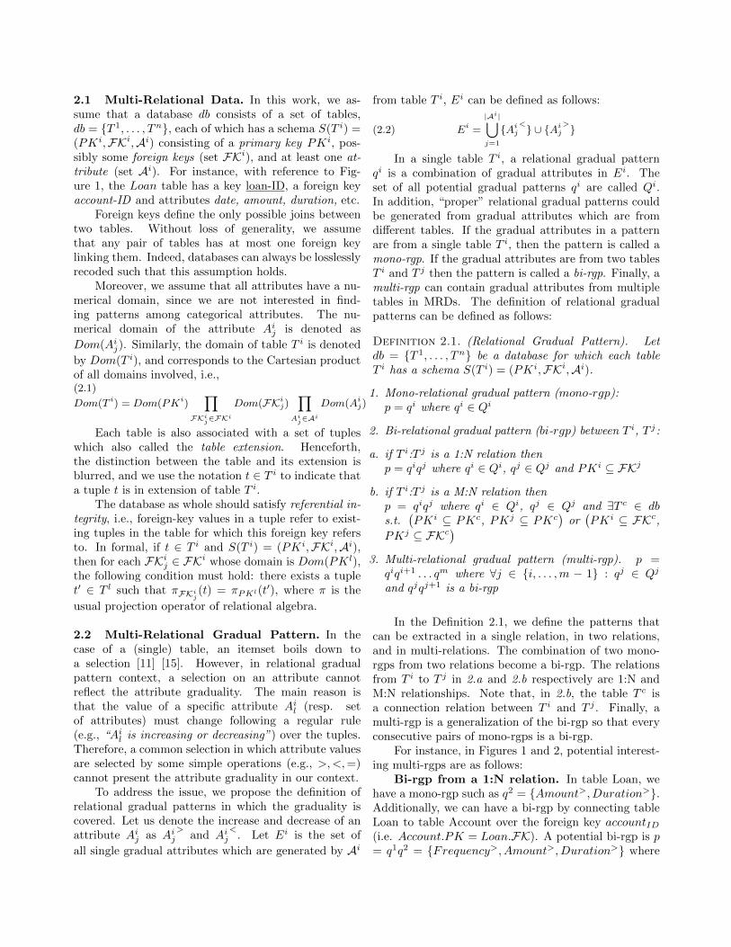
2.1 Multi-Relational Data. In this work, we as-sume that a database db consists of a set of tables,db = {T 1, . . . , Tn}, each of which has a schema S(T i) =(PKi,FKi,Ai) consisting of a primary key PKi, pos-sibly some foreign keys (set FKi), and at least one at-tribute (set Ai). For instance, with reference to Fig-ure 1, the Loan table has a key loan-ID, a foreign keyaccount-ID and attributes date, amount, duration, etc.

Foreign keys define the only possible joins betweentwo tables. Without loss of generality, we assumethat any pair of tables has at most one foreign keylinking them. Indeed, databases can always be losslesslyrecoded such that this assumption holds.

Moreover, we assume that all attributes have a nu-merical domain, since we are not interested in find-ing patterns among categorical attributes. The nu-merical domain of the attribute Aij is denoted as

Dom(Aij). Similarly, the domain of table T i is denoted

by Dom(T i), and corresponds to the Cartesian productof all domains involved, i.e.,(2.1)

Dom(T i) = Dom(PKi)∏

FKij∈FKi

Dom(FKij)∏

Aij∈Ai

Dom(Aij)

Each table is also associated with a set of tupleswhich also called the table extension. Henceforth,the distinction between the table and its extension isblurred, and we use the notation t ∈ T i to indicate thata tuple t is in extension of table T i.

The database as whole should satisfy referential in-tegrity, i.e., foreign-key values in a tuple refer to exist-ing tuples in the table for which this foreign key refersto. In formal, if t ∈ T i and S(T i) = (PKi,FKi,Ai),then for each FKij ∈ FK

i whose domain is Dom(PKl),the following condition must hold: there exists a tuplet′ ∈ T l such that πFKij (t) = πPKl(t′), where π is the

usual projection operator of relational algebra.

2.2 Multi-Relational Gradual Pattern. In thecase of a (single) table, an itemset boils down toa selection [11] [15]. However, in relational gradualpattern context, a selection on an attribute cannotreflect the attribute graduality. The main reason isthat the value of a specific attribute Ail (resp. setof attributes) must change following a regular rule(e.g., “Ail is increasing or decreasing”) over the tuples.Therefore, a common selection in which attribute valuesare selected by some simple operations (e.g., >,<,=)cannot present the attribute graduality in our context.

To address the issue, we propose the definition ofrelational gradual patterns in which the graduality iscovered. Let us denote the increase and decrease of anattribute Aij as Aij

>and Aij

<. Let Ei is the set of

all single gradual attributes which are generated by Ai

from table T i, Ei can be defined as follows:

(2.2) Ei =

|Ai|⋃j=1

{Aij<} ∪ {Aij

>}

In a single table T i, a relational gradual patternqi is a combination of gradual attributes in Ei. Theset of all potential gradual patterns qi are called Qi.In addition, “proper” relational gradual patterns couldbe generated from gradual attributes which are fromdifferent tables. If the gradual attributes in a patternare from a single table T i, then the pattern is called amono-rgp. If the gradual attributes are from two tablesT i and T j then the pattern is called a bi-rgp. Finally, amulti-rgp can contain gradual attributes from multipletables in MRDs. The definition of relational gradualpatterns can be defined as follows:

Definition 2.1. (Relational Gradual Pattern). Letdb = {T 1, . . . , Tn} be a database for which each tableT i has a schema S(T i) = (PKi,FKi,Ai).

1. Mono-relational gradual pattern (mono-rgp):p = qi where qi ∈ Qi

2. Bi-relational gradual pattern (bi-rgp) between T i, T j:

a. if T i:T j is a 1:N relation thenp = qiqj where qi ∈ Qi, qj ∈ Qj and PKi ⊆ FKj

b. if T i:T j is a M:N relation thenp = qiqj where qi ∈ Qi, qj ∈ Qj and ∃T c ∈ dbs.t.

(PKi ⊆ PKc, PKj ⊆ PKc

)or(PKi ⊆ FKc,

PKj ⊆ FKc)

3. Multi-relational gradual pattern (multi-rgp). p =qiqi+1 . . . qm where ∀j ∈ {i, . . . ,m − 1} : qj ∈ Qj

and qjqj+1 is a bi-rgp

In the Definition 2.1, we define the patterns thatcan be extracted in a single relation, in two relations,and in multi-relations. The combination of two mono-rgps from two relations become a bi-rgp. The relationsfrom T i to T j in 2.a and 2.b respectively are 1:N andM:N relationships. Note that, in 2.b, the table T c isa connection relation between T i and T j . Finally, amulti-rgp is a generalization of the bi-rgp so that everyconsecutive pairs of mono-rgps is a bi-rgp.

For instance, in Figures 1 and 2, potential interest-ing multi-rgps are as follows:

Bi-rgp from a 1:N relation. In table Loan, wehave a mono-rgp such as q2 = {Amount>, Duration>}.Additionally, we can have a bi-rgp by connecting tableLoan to table Account over the foreign key accountID(i.e. Account.PK = Loan.FK). A potential bi-rgp is p= q1q2 = {Frequency>, Amount>, Duration>} where

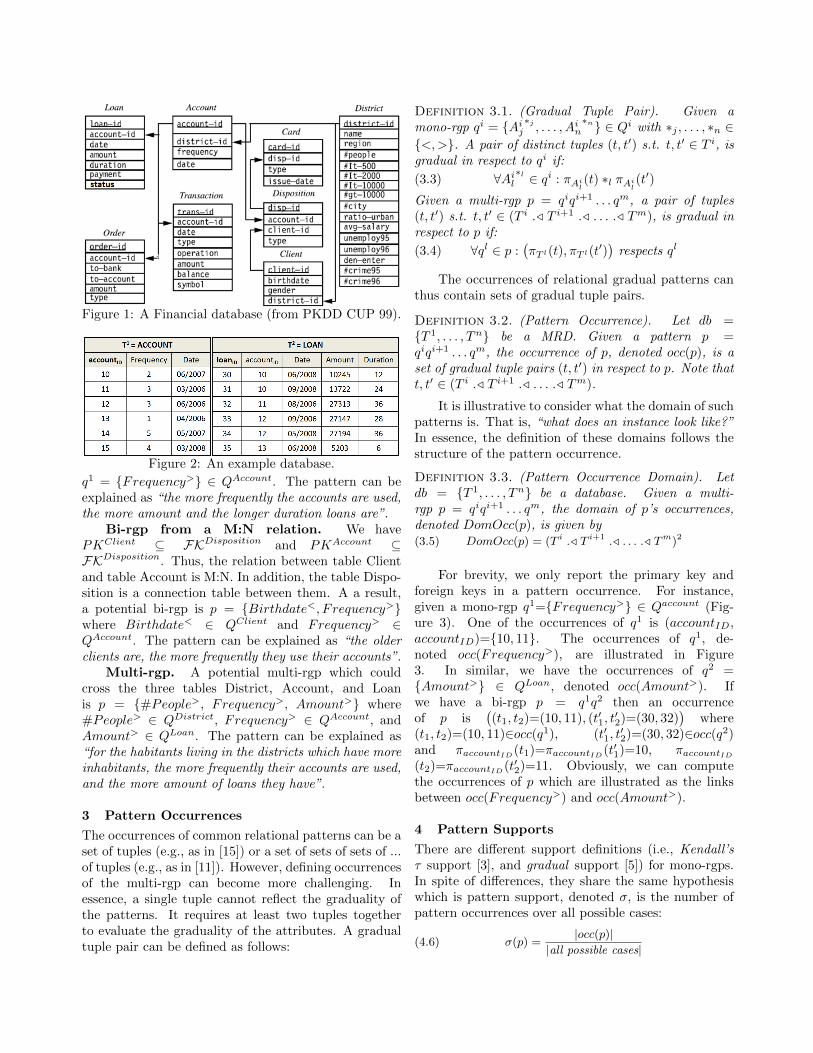
Figure 1: A Financial database (from PKDD CUP 99).

Figure 2: An example database.

q1 = {Frequency>} ∈ QAccount. The pattern can beexplained as “the more frequently the accounts are used,the more amount and the longer duration loans are”.

Bi-rgp from a M:N relation. We havePKClient ⊆ FKDisposition and PKAccount ⊆FKDisposition. Thus, the relation between table Clientand table Account is M:N. In addition, the table Dispo-sition is a connection table between them. A a result,a potential bi-rgp is p = {Birthdate<, F requency>}where Birthdate< ∈ QClient and Frequency> ∈QAccount. The pattern can be explained as “the olderclients are, the more frequently they use their accounts”.

Multi-rgp. A potential multi-rgp which couldcross the three tables District, Account, and Loanis p = {#People>, F requency>, Amount>} where#People> ∈ QDistrict, F requency> ∈ QAccount, andAmount> ∈ QLoan. The pattern can be explained as“for the habitants living in the districts which have moreinhabitants, the more frequently their accounts are used,and the more amount of loans they have”.

3 Pattern Occurrences

The occurrences of common relational patterns can be aset of tuples (e.g., as in [15]) or a set of sets of sets of ...of tuples (e.g., as in [11]). However, defining occurrencesof the multi-rgp can become more challenging. Inessence, a single tuple cannot reflect the graduality ofthe patterns. It requires at least two tuples togetherto evaluate the graduality of the attributes. A gradualtuple pair can be defined as follows:

Definition 3.1. (Gradual Tuple Pair). Given amono-rgp qi = {Aij

∗j , . . . , Ain∗n} ∈ Qi with ∗j , . . . , ∗n ∈

{<,>}. A pair of distinct tuples (t, t′) s.t. t, t′ ∈ T i, isgradual in respect to qi if:

(3.3) ∀Ail∗l ∈ qi : πAil (t) ∗l πAil (t

′)

Given a multi-rgp p = qiqi+1 . . . qm, a pair of tuples(t, t′) s.t. t, t′ ∈ (T i ./ T i+1 ./ . . . ./ Tm), is gradual inrespect to p if:

(3.4) ∀ql ∈ p :(πT l(t), πT l(t

′))

respects ql

The occurrences of relational gradual patterns canthus contain sets of gradual tuple pairs.

Definition 3.2. (Pattern Occurrence). Let db ={T 1, . . . , Tn} be a MRD. Given a pattern p =qiqi+1 . . . qm, the occurrence of p, denoted occ(p), is aset of gradual tuple pairs (t, t′) in respect to p. Note thatt, t′ ∈ (T i ./ T i+1 ./ . . . ./ Tm).

It is illustrative to consider what the domain of suchpatterns is. That is, “what does an instance look like?”In essence, the definition of these domains follows thestructure of the pattern occurrence.

Definition 3.3. (Pattern Occurrence Domain). Letdb = {T 1, . . . , Tn} be a database. Given a multi-rgp p = qiqi+1 . . . qm, the domain of p’s occurrences,denoted DomOcc(p), is given by(3.5) DomOcc(p) = (T i ./ T i+1 ./ . . . ./ Tm)2

For brevity, we only report the primary key andforeign keys in a pattern occurrence. For instance,given a mono-rgp q1={Frequency>} ∈ Qaccount (Fig-ure 3). One of the occurrences of q1 is (accountID,accountID)={10, 11}. The occurrences of q1, de-noted occ(Frequency>), are illustrated in Figure3. In similar, we have the occurrences of q2 ={Amount>} ∈ QLoan, denoted occ(Amount>). Ifwe have a bi-rgp p = q1q2 then an occurrenceof p is

((t1, t2)=(10, 11), (t′1, t

′2)=(30, 32)

)where

(t1, t2)=(10, 11)∈occ(q1), (t′1, t′2)=(30, 32)∈occ(q2)

and πaccountID (t1)=πaccountID (t′1)=10, πaccountID(t2)=πaccountID (t′2)=11. Obviously, we can computethe occurrences of p which are illustrated as the linksbetween occ(Frequency>) and occ(Amount>).

4 Pattern Supports

There are different support definitions (i.e., Kendall’sτ support [3], and gradual support [5]) for mono-rgps.In spite of differences, they share the same hypothesiswhich is pattern support, denoted σ, is the number ofpattern occurrences over all possible cases:

(4.6) σ(p) =|occ(p)|

|all possible cases|

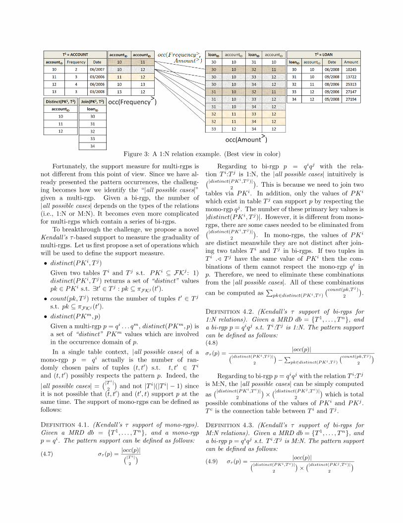
Figure 3: A 1:N relation example. (Best view in color)

Fortunately, the support measure for multi-rgps isnot different from this point of view. Since we have al-ready presented the pattern occurrences, the challeng-ing becomes how we identify the “|all possible cases|”given a multi-rgp. Given a bi-rgp, the number of|all possible cases| depends on the types of the relations(i.e., 1:N or M:N). It becomes even more complicatedfor multi-rgps which contain a series of bi-rgps.

To breakthrough the challenge, we propose a novelKendall’s τ -based support to measure the graduality ofmulti-rgps. Let us first propose a set of operations whichwill be used to define the support measure.

• distinct(PKi, T j)

Given two tables T i and T j s.t. PKi ⊆ FKj : 1)distinct(PKi, T j) returns a set of “distinct” valuespk ∈ PKi s.t. ∃t′ ∈ T j : pk ⊆ πFKj (t′).

• count(pk, T j) returns the number of tuples t′ ∈ T js.t. pk ⊆ πFKj (t′).• distinct(PKm, p)

Given a multi-rgp p = qi . . . qm, distinct(PKm, p) isa set of “distinct” PKm values which are involvedin the occurrence domain of p.

In a single table context, |all possible cases| of amono-rgp p = qi actually is the number of ran-domly chosen pairs of tuples (t, t′) s.t. t, t′ ∈ T i

and (t, t′) possibly respects the pattern p. Indeed, the

|all possible cases| =(|T i|

2

)and not |T i|(|T i| − 1) since

it is not possible that (t, t′) and (t′, t) support p at thesame time. The support of mono-rgps can be defined asfollows:

Definition 4.1. (Kendall’s τ support of mono-rgps).Given a MRD db = {T 1, . . . , Tn}, and a mono-rgpp = qi. The pattern support can be defined as follows:

(4.7) στ (p) =|occ(p)|(|T i|

2

)

Regarding to bi-rgp p = qiqj with the rela-tion T i:T j is 1:N, the |all possible cases| intuitively is(|distinct(PKi,T j)|

2

). This is because we need to join two

tables via PKi. In addition, only the values of PKi

which exist in table T j can support p by respecting themono-rgp qj . The number of these primary key values is|distinct(PKi, T j)|. However, it is different from mono-rgps, there are some cases needed to be eliminated from(|distinct(PKi,T j)|

2

). In mono-rgps, the values of PKi

are distinct meanwhile they are not distinct after join-ing two tables T i and T j in bi-rgps. If two tuples inT i ./ T j have the same value of PKi then the com-binations of them cannot respect the mono-rgp qi inp. Therefore, we need to eliminate these combinationsfrom the |all possible cases|. All of these combinations

can be computed as∑pk∈distinct(PKi,T j)

(count(pk,T j)2

).

Definition 4.2. (Kendall’s τ support of bi-rgps for1:N relations). Given a MRD db = {T 1, . . . , Tn}, anda bi-rgp p = qiqj s.t. T i:T j is 1:N. The pattern supportcan be defined as follows:(4.8)

στ (p) =|occ(p)|(|distinct(PKi,T j)|

2

)−

∑pk∈distinct(PKi,T j)

(count(pk,T j)2

)Regarding to bi-rgp p = qiqj with the relation T i:T j

is M:N, the |all possible cases| can be simply computed

as(|distinct(PKi,T c)|

2

)×(|distinct(PKj ,T c)|

2

)which is total

possible combinations of the values of PKi and PKj .T c is the connection table between T i and T j .

Definition 4.3. (Kendall’s τ support of bi-rgps forM:N relations). Given a MRD db = {T 1, . . . , Tn}, anda bi-rgp p = qiqj s.t. T i:T j is M:N. The pattern supportcan be defined as follows:

(4.9) στ (p) =|occ(p)|(|distinct(PKi,Tc)|

2

)×(|distinct(PKj ,Tc)|

2

)

The support of multi-rgps can be considered asa generalization of bi-rgps. Given a multi-rgp p =qi . . . qm, p can be rewrote as p = (qi . . . qm−1)qm.In fact, (qi . . . qm−1) can be considered as a mono-rgpwhose domain is T i ./ . . . ./ Tm−1 and qm is anothermono-rgp. So, the |all possible cases| clearly dependson the relationship between two tables Tm−1 and Tm.As a result, the Definitions 4.2, 4.3 can be utilized tocompute the support for multi-rgps. What we need is toidentify values of the primary key PKm−1 which exist inthe occ(qi . . . qm−1). The set of these values are denotedas PKp′= distinct(PKm−1, p′) where p′ = qi . . . qm−1.The support of multi-rgps can be defined as follows:

Definition 4.4. (Kendall’s τ support of multi-rgps).Let db = {T 1, . . . , Tn} be a database, the support ofmulti-rgps p = qi . . . qm−1qm can be defined as follows:

1) if Tm−1:Tm is 1:N

στ (p) =|occ(p)|(|distinct(PKp′ ,Tm)|

2

)−∑pk∈distinct(PKp′ ,Tm)

(count(pk,Tm)

2

)2) if Tm−1:Tm is M:N and T c is the connection table

στ (p) = |occ(p)|(|distinct(PKp′ ,Tc)|2

)×(|distinct(PKm,Tc)|

2

)In practice, to reduce the memory consumption

we index only the tuples exist in the occurrences of(qi . . . qm−1). The following theorem gives the expectedστ , denoted E[στ ], in the case of statistically indepen-dent attributes. This expected support can be used asa reference point to assess the quality of a multi-rgp.

Theorem 4.1. (E[στ ]). Given a set of statisticallyindependent gradual attributes s = {A1, A2, . . . , An},Ps = {p1, . . . , pm} is the set of all possible independentmulti-rgps generated from s. The expected suppτ of apattern p ∈ Ps is E[στ ](p) = 1

(2n−1+n(3n−1−1)+1) .

where p and p′ are independent multi-rgps if(DomOcc(p) = DomOcc(p′)) ∧ (occ(p) ∩ occ(p′) = ∅).

The proof of Theorem 4.1 is available at https:

//sites.google.com/site/ihaiphan/. Until now, wehave proposed the definition of Kendall’s τ support ofmulti-rgps. In [5], Di-Jorio et. al. propose a gradualsupport measure to emphasize the consecutiveness inchanging of attributes over the values. Instead of a pairof tuples, the gradual support concerns on a list of tuplesL = {ti, ti+1, . . . , tk} in which ∀tj , tj+1 ∈ L : (tj , tj+1)is a gradual tuple pair (Def. 3.1). In the gradualsupport, |occ(p)| becomes the size of the maximal listof tuples L which supports p in the MRD db. The|all possible cases| becomes the possible longest L in thedb. Based on this idea, we also propose the gradualsupport, denoted σg(p), for multi-rgps.

5 Multi-Relational Gradual Pattern Miner

Extracting the complete set of multi-rgps is a non-trivialtask. At first glance, the number of potential multi-rgpsis exponential, i.e., approximately 22×|Adb| where Adb isa set of all numerical attributes in the MRD db.

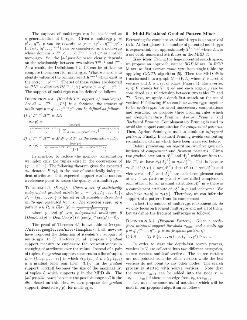
Key idea. Facing the huge potential search space,we propose an approach, named RGP Miner. In RGPMiner, we first extract mono-rgps from single tables byapplying GRITE algorithm [5]. Then the MRD db istransformed into a graph G = (V,E) where V is a set ofvertices and E is a set of edges (Figure 4). Each vertexvi ∈ V stands for T i ∈ db and each edge eij can beconsidered as a relationship between two tables T i andT j . Next, we apply a depth-first search on the set ofvertices V following E to combine mono-rgps togetherto be multi-rgps. To avoid unnecessary computationsand searches, we propose three pruning rules whichare Complementary Pruning, Apriori Pruning, andBackward Pruning. Complementary Pruning is used toavoid the support computation for complement patterns.Then, Apriori Pruning is used to eliminate infrequentpatterns. Finally, Backward Pruning avoids computingredundant patterns which have been traversed before.

Before presenting our algorithm, we first give def-initions of complement and frequent patterns. Giventwo gradual attributes Aij

>and Aij

<which are from ta-

ble T i, we have στ (Aij>

) = στ (Aij<

). This is because

∀t, t′ : if (t, t′) ∈ occ(Aij>

) then (t′, t) ∈ occ(Aij<

) and

vice versa. Aij>

and Aij<

are called complement eachother. Two patterns p and p′ are called complementeach other if for all gradual attributes Aij

∗in p there is

a complement attribute of Aij∗

in p′ and vice versa. Wealso have στ (p) = στ (p′). Therefore, we can infer thesupport of a pattern from its complement.

In fact, the number of multi-rgps is exponential. Sowe only focus on frequent multi-rgps and not all of them.Let us define the frequent multi-rgps as follows:

Definition 5.1. (Frequent Pattern). Given a prede-fined minimal support threshold σmin, and a multi-rgpp = qiqi+1 . . . qm. p is an frequent pattern if:

(5.10) ∀j ∈ {i, . . . ,m} : στ (qi . . . qj) ≥ σmin

In order to start the depth-first search process,vertices in V are collected into two different categories,source vertices and leaf vertices. The source verticesare not pointed from the other vertices while the leafvertices do not point to any other nodes. The searchprocess is started with source vertices. Note thatthe vertex vm+1 can be added into the node r ={vi, . . . , vm} if there is an edge from vm to vm+1.

Let us define some useful notations which will beused in our proposed algorithm as follows:

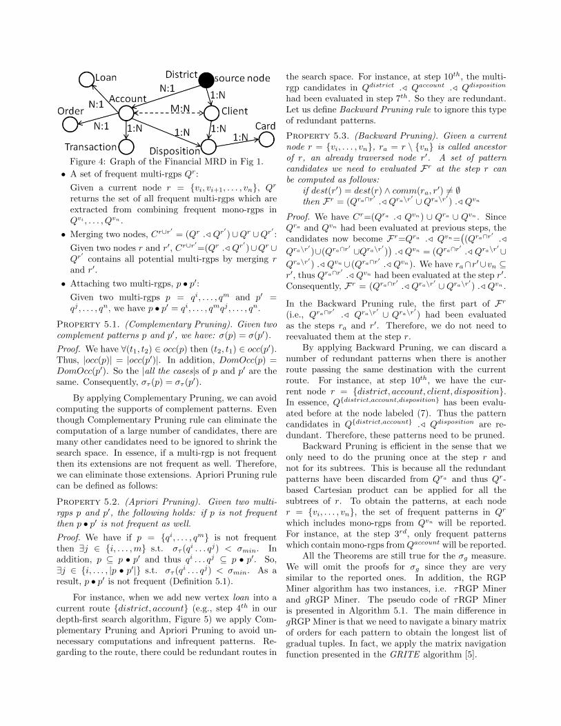
Figure 4: Graph of the Financial MRD in Fig 1.

• A set of frequent multi-rgps Qr:

Given a current node r = {vi, vi+1, . . . , vn}, Qr

returns the set of all frequent multi-rgps which areextracted from combining frequent mono-rgps inQvi , . . . , Qvn .

• Merging two nodes, Cr∪r′

= (Qr ./ Qr′)∪Qr ∪Qr′ :

Given two nodes r and r′, Cr∪r′=(Qr ./ Qr

′)∪Qr ∪

Qr′

contains all potential multi-rgps by merging rand r′.

• Attaching two multi-rgps, p • p′:Given two multi-rgps p = qi, . . . , qm and p′ =qj , . . . , qn, we have p • p′ = qi, . . . , qmqj , . . . , qn.

Property 5.1. (Complementary Pruning). Given twocomplement patterns p and p′, we have: σ(p) = σ(p′).

Proof. We have ∀(t1, t2) ∈ occ(p) then (t2, t1) ∈ occ(p′).Thus, |occ(p)| = |occ(p′)|. In addition, DomOcc(p) =DomOcc(p′). So the |all the cases|s of p and p′ are thesame. Consequently, στ (p) = στ (p′).

By applying Complementary Pruning, we can avoidcomputing the supports of complement patterns. Eventhough Complementary Pruning rule can eliminate thecomputation of a large number of candidates, there aremany other candidates need to be ignored to shrink thesearch space. In essence, if a multi-rgp is not frequentthen its extensions are not frequent as well. Therefore,we can eliminate those extensions. Apriori Pruning rulecan be defined as follows:

Property 5.2. (Apriori Pruning). Given two multi-rgps p and p′, the following holds: if p is not frequentthen p • p′ is not frequent as well.

Proof. We have if p = {qi, . . . , qm} is not frequentthen ∃j ∈ {i, . . . ,m} s.t. στ (qi . . . qj) < σmin. Inaddition, p ⊆ p • p′ and thus qi . . . qj ⊆ p • p′. So,∃j ∈ {i, . . . , |p • p′|} s.t. στ (qi . . . qj) < σmin. As aresult, p • p′ is not frequent (Definition 5.1).

For instance, when we add new vertex loan into acurrent route {district, account} (e.g., step 4th in ourdepth-first search algorithm, Figure 5) we apply Com-plementary Pruning and Apriori Pruning to avoid un-necessary computations and infrequent patterns. Re-garding to the route, there could be redundant routes in

the search space. For instance, at step 10th, the multi-rgp candidates in Qdistrict ./ Qaccount ./ Qdisposition

had been evaluated in step 7th. So they are redundant.Let us define Backward Pruning rule to ignore this typeof redundant patterns.

Property 5.3. (Backward Pruning). Given a currentnode r = {vi, . . . , vn}, ra = r \ {vn} is called ancestorof r, an already traversed node r′. A set of patterncandidates we need to evaluated Fr at the step r canbe computed as follows:

if dest(r′) = dest(r) ∧ comm(ra, r′) 6= ∅

then Fr = (Qra∩r′./ Qra\r

′ ∪Qra\r′) ./ Qvn

Proof. We have Cr=(Qra ./ Qvn) ∪ Qra ∪ Qvn . SinceQra and Qvn had been evaluated at previous steps, thecandidates now become Fr=Qra ./ Qvn=

((Qra∩r

′./

Qra\r′)∪(Qra∩r

′ ∪Qra\r′))./ Qvn = (Qra∩r

′./ Qra\r

′∪Qra\r

′) ./ Qvn ∪ (Qra∩r

′./ Qvn). We have ra∩r′∪vn ⊆

r′, thus Qra∩r′./ Qvn had been evaluated at the step r′.

Consequently, Fr = (Qra∩r′./ Qra\r

′ ∪Qra\r′) ./ Qvn .

In the Backward Pruning rule, the first part of Fr(i.e., Qra∩r

′./ Qra\r

′ ∪ Qra\r′) had been evaluatedas the steps ra and r′. Therefore, we do not need toreevaluated them at the step r.

By applying Backward Pruning, we can discard anumber of redundant patterns when there is anotherroute passing the same destination with the currentroute. For instance, at step 10th, we have the cur-rent node r = {district, account, client, disposition}.In essence, Q{district,account,disposition} has been evalu-ated before at the node labeled (7). Thus the patterncandidates in Q{district,account} ./ Qdisposition are re-dundant. Therefore, these patterns need to be pruned.

Backward Pruning is efficient in the sense that weonly need to do the pruning once at the step r andnot for its subtrees. This is because all the redundantpatterns have been discarded from Qra and thus Qr-based Cartesian product can be applied for all thesubtrees of r. To obtain the patterns, at each noder = {vi, . . . , vn}, the set of frequent patterns in Qr

which includes mono-rgps from Qvn will be reported.For instance, at the step 3rd, only frequent patternswhich contain mono-rgps fromQaccount will be reported.

All the Theorems are still true for the σg measure.We will omit the proofs for σg since they are verysimilar to the reported ones. In addition, the RGPMiner algorithm has two instances, i.e. τRGP Minerand gRGP Miner. The pseudo code of τRGP Mineris presented in Algorithm 5.1. The main difference ingRGP Miner is that we need to navigate a binary matrixof orders for each pattern to obtain the longest list ofgradual tuples. In fact, we apply the matrix navigationfunction presented in the GRITE algorithm [5].

Algorithm 5.1. τRGP MinerInput: MRD db, source nodes S, G={V,E}, σminOutput: all frequent multi-rgps

1 begin2 R := ∅;foreach v ∈ S do

3 r := {v};RGpattern(db, r, v,G, σmin);

4 RGpattern(db, r, v,G, σmin)begin

5 foreach node l ∈ v.edges do6 combining(r, v, l);7 output Qv ; delete Qv; R := R ∪ r;8 combining(route r, node v, node l)

begin9 if type(v, l) = 1 : N then

10 denom := (|join(PKv,l)|

2 );11 else

12 denom := (|distinct(PKv,k)|

2 )× (|distinct(PKl,k)|

2 );13 temp = ∅;

foreach pattern qi ∈ Qv do14 if Backward(qi, l, r, R) = true then15 if exist(db, qi) = false then16 create(db, qi);

17 foreach pattern qj ∈ Ql do18 if complement(qiqj , temp) = false then19 create(db, qj);

occ := |qi ./ qj |;στ (q

iqj) := occdenom ;

if στ (qiqj) ≥ σmin then

20 temp := temp ∪ qiqj ;21 delete qj ;

22 else23 temp := temp ∪ qiqj ;24 delete qi;

25 Ql := Ql ∪ temp;RGpattern(db, r ∪ l, l, G, σmin);

26 type(v, l) is the connection type v:l, exist(db, qi) returns true

if qi exists in db, return false otherwise, complement(qiqj , temp)

returns false if there is no complement of qiqj in temp.

6 Experimental Results

A comprehensive experiment study has been conductedon real datasets which are the Financial data1 (PKDDCup 99) and the Thrombosis data1 (PKDD Cup 2001).The Financial database scheme corresponds to the onegiven in Figure 1. There are 4,500 accounts, 5,369clients, 5,369 objects in disposition, 6,471 objects inorder, 2,500 objects in transaction, 682 objects in loan,892 cards, and 77 districts. The experiments are carriedout on a 2.8GHz Intel Core i7 cpu, 4GB memory.

6.1 Patterns. Interesting multi-rgps were discoveredin the Financial database and Table 1 illustrates topstrongest and longest patterns. We discuss some of themin the following.

Bases on στ . The τRGP Miner returns thepattern p = {district.Unemploy96<, order.Amount>}with στ (p) = 58.32%. The pattern could be explainedas: “the less unemployed ratio districts are, the moreexpensive orders the habitants, who live in the districts,

1http://lisp.vse.cz/challenge/.

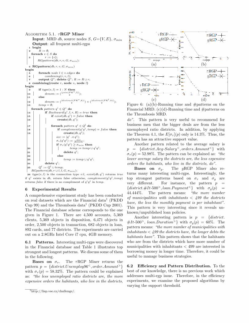
(a) (b)

(c) (d)Figure 6: (a)(b)-Running time and #patterns on theFinancial MRD. (c)(d)-Running time and #patterns onthe Thrombosis MRD.

do”. This pattern is very useful to recommend forbusiness men that the bigger deals are from the lessunemployed ratio districts. In addition, by applyingthe Theorem 4.1, the E[στ ](p) only is 14.3%. Thus, thepattern has an attractive support value.

Another pattern related to the average salary isp = {district.Avg-Salary<, orders.Amount<} withστ (p) = 52.98%. The pattern can be explained as: “thelower average salary the districts are, the less expensiveorders the habitants, who live in the districts, do”.

Bases on σg. The gRGP Miner also re-turns many interesting multi-rgps. Interestingly, thetop strongest patterns based on στ and σg arevery different. For instance, the pattern p ={district.#It-500>, loan.Payment<} with σg(p) =44.444%. The pattern means: “the more numberof municipalities with inhabitants < 499 the districtshave, the less the monthly payment is per inhabitant”.This pattern is very interesting since it reveals un-known/unpublished loan policies.

Another interesting pattern is p = {district.#It-500>, loan.Duration>} with σg(p) = 60%. Thepattern means: “the more number of municipalities withinhabitants < 499 the districts have, the longer debts thehabitants have”. This pattern shows that the habitantswho are from the districts which have more number ofmunicipalities with inhabitants < 499 are interested inborrowing money in longer time. Therefore, it could beuseful to manage business strategies.

6.2 Efficiency and Pattern Distribution. To thebest of our knowledge, there is no previous work whichaddresses multi-rgp issue. Therefore, in the efficiencyexperiments, we examine the proposed algorithms byvarying the support threshold.

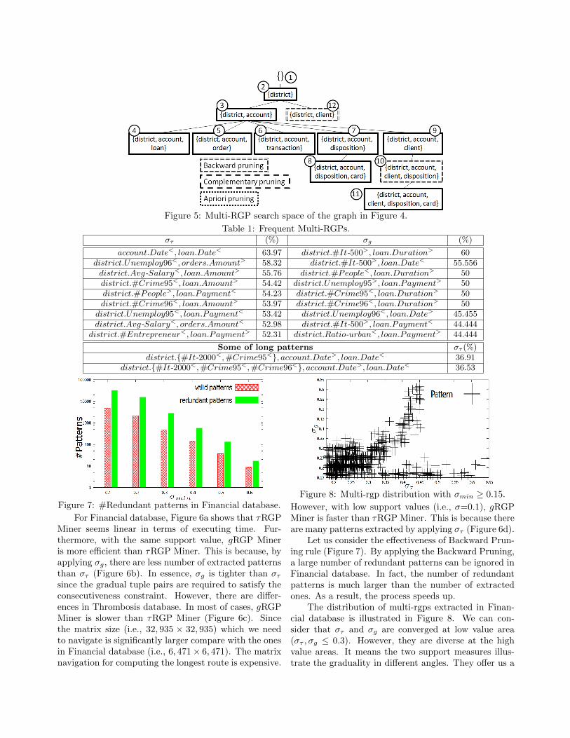
Figure 5: Multi-RGP search space of the graph in Figure 4.

Table 1: Frequent Multi-RGPs.στ (%) σg (%)

account.Date<, loan.Date< 63.97 district.#It-500>, loan.Duration> 60district.Unemploy96<, orders.Amount> 58.32 district.#It-500>, loan.Date< 55.556district.Avg-Salary<, loan.Amount> 55.76 district.#People<, loan.Duration> 50district.#Crime95<, loan.Amount> 54.42 district.Unemploy95>, loan.Payment> 50district.#People>, loan.Payment< 54.23 district.#Crime95<, loan.Duration> 50district.#Crime96<, loan.Amount> 53.97 district.#Crime96<, loan.Duration> 50district.Unemploy95<, loan.Payment< 53.42 district.Unemploy96<, loan.Date> 45.455district.Avg-Salary<, orders.Amount< 52.98 district.#It-500>, loan.Payment< 44.444

district.#Entrepreneur<, loan.Payment> 52.31 district.Ratio-urban<, loan.Payment> 44.444

Some of long patterns στ (%)district.{#It-2000<,#Crime95<}, account.Date>, loan.Date< 36.91

district.{#It-2000<,#Crime95<,#Crime96<}, account.Date>, loan.Date< 36.53

Figure 7: #Redundant patterns in Financial database.

For Financial database, Figure 6a shows that τRGPMiner seems linear in terms of executing time. Fur-thermore, with the same support value, gRGP Mineris more efficient than τRGP Miner. This is because, byapplying σg, there are less number of extracted patternsthan στ (Figure 6b). In essence, σg is tighter than στsince the gradual tuple pairs are required to satisfy theconsecutiveness constraint. However, there are differ-ences in Thrombosis database. In most of cases, gRGPMiner is slower than τRGP Miner (Figure 6c). Sincethe matrix size (i.e., 32, 935 × 32, 935) which we needto navigate is significantly larger compare with the onesin Financial database (i.e., 6, 471× 6, 471). The matrixnavigation for computing the longest route is expensive.

Figure 8: Multi-rgp distribution with σmin ≥ 0.15.

However, with low support values (i.e., σ=0.1), gRGPMiner is faster than τRGP Miner. This is because thereare many patterns extracted by applying στ (Figure 6d).

Let us consider the effectiveness of Backward Prun-ing rule (Figure 7). By applying the Backward Pruning,a large number of redundant patterns can be ignored inFinancial database. In fact, the number of redundantpatterns is much larger than the number of extractedones. As a result, the process speeds up.

The distribution of multi-rgps extracted in Finan-cial database is illustrated in Figure 8. We can con-sider that στ and σg are converged at low value area(στ , σg ≤ 0.3). However, they are diverse at the highvalue areas. It means the two support measures illus-trate the graduality in different angles. They offer us a

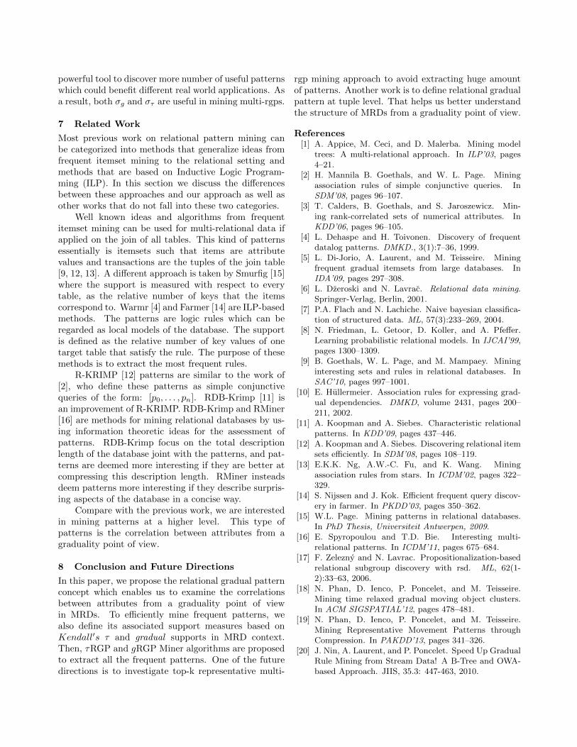
powerful tool to discover more number of useful patternswhich could benefit different real world applications. Asa result, both σg and στ are useful in mining multi-rgps.

7 Related Work

Most previous work on relational pattern mining canbe categorized into methods that generalize ideas fromfrequent itemset mining to the relational setting andmethods that are based on Inductive Logic Program-ming (ILP). In this section we discuss the differencesbetween these approaches and our approach as well asother works that do not fall into these two categories.

Well known ideas and algorithms from frequentitemset mining can be used for multi-relational data ifapplied on the join of all tables. This kind of patternsessentially is itemsets such that items are attributevalues and transactions are the tuples of the join table[9, 12, 13]. A different approach is taken by Smurfig [15]where the support is measured with respect to everytable, as the relative number of keys that the itemscorrespond to. Warmr [4] and Farmer [14] are ILP-basedmethods. The patterns are logic rules which can beregarded as local models of the database. The supportis defined as the relative number of key values of onetarget table that satisfy the rule. The purpose of thesemethods is to extract the most frequent rules.

R-KRIMP [12] patterns are similar to the work of[2], who define these patterns as simple conjunctivequeries of the form: [p0, . . . , pn]. RDB-Krimp [11] isan improvement of R-KRIMP. RDB-Krimp and RMiner[16] are methods for mining relational databases by us-ing information theoretic ideas for the assessment ofpatterns. RDB-Krimp focus on the total descriptionlength of the database joint with the patterns, and pat-terns are deemed more interesting if they are better atcompressing this description length. RMiner insteadsdeem patterns more interesting if they describe surpris-ing aspects of the database in a concise way.

Compare with the previous work, we are interestedin mining patterns at a higher level. This type ofpatterns is the correlation between attributes from agraduality point of view.

8 Conclusion and Future Directions

In this paper, we propose the relational gradual patternconcept which enables us to examine the correlationsbetween attributes from a graduality point of viewin MRDs. To efficiently mine frequent patterns, wealso define its associated support measures based onKendall′s τ and gradual supports in MRD context.Then, τRGP and gRGP Miner algorithms are proposedto extract all the frequent patterns. One of the futuredirections is to investigate top-k representative multi-

rgp mining approach to avoid extracting huge amountof patterns. Another work is to define relational gradualpattern at tuple level. That helps us better understandthe structure of MRDs from a graduality point of view.

References[1] A. Appice, M. Ceci, and D. Malerba. Mining model

trees: A multi-relational approach. In ILP’03, pages4–21.

[2] H. Mannila B. Goethals, and W. L. Page. Miningassociation rules of simple conjunctive queries. InSDM’08, pages 96–107.

[3] T. Calders, B. Goethals, and S. Jaroszewicz. Min-ing rank-correlated sets of numerical attributes. InKDD’06, pages 96–105.

[4] L. Dehaspe and H. Toivonen. Discovery of frequentdatalog patterns. DMKD., 3(1):7–36, 1999.

[5] L. Di-Jorio, A. Laurent, and M. Teisseire. Miningfrequent gradual itemsets from large databases. InIDA’09, pages 297–308.

[6] L. Dzeroski and N. Lavrac. Relational data mining.Springer-Verlag, Berlin, 2001.

[7] P.A. Flach and N. Lachiche. Naive bayesian classifica-tion of structured data. ML, 57(3):233–269, 2004.

[8] N. Friedman, L. Getoor, D. Koller, and A. Pfeffer.Learning probabilistic relational models. In IJCAI’99,pages 1300–1309.

[9] B. Goethals, W. L. Page, and M. Mampaey. Mininginteresting sets and rules in relational databases. InSAC’10, pages 997–1001.

[10] E. Hullermeier. Association rules for expressing grad-ual dependencies. DMKD, volume 2431, pages 200–211, 2002.

[11] A. Koopman and A. Siebes. Characteristic relationalpatterns. In KDD’09, pages 437–446.

[12] A. Koopman and A. Siebes. Discovering relational itemsets efficiently. In SDM’08, pages 108–119.

[13] E.K.K. Ng, A.W.-C. Fu, and K. Wang. Miningassociation rules from stars. In ICDM’02, pages 322–329.

[14] S. Nijssen and J. Kok. Efficient frequent query discov-ery in farmer. In PKDD’03, pages 350–362.

[15] W.L. Page. Mining patterns in relational databases.In PhD Thesis, Universiteit Antwerpen, 2009.

[16] E. Spyropoulou and T.D. Bie. Interesting multi-relational patterns. In ICDM’11, pages 675–684.

[17] F. Zelezny and N. Lavrac. Propositionalization-basedrelational subgroup discovery with rsd. ML, 62(1-2):33–63, 2006.

[18] N. Phan, D. Ienco, P. Poncelet, and M. Teisseire.Mining time relaxed gradual moving object clusters.In ACM SIGSPATIAL’12, pages 478–481.

[19] N. Phan, D. Ienco, P. Poncelet, and M. Teisseire.Mining Representative Movement Patterns throughCompression. In PAKDD’13, pages 341–326.

[20] J. Nin, A. Laurent, and P. Poncelet. Speed Up GradualRule Mining from Stream Data! A B-Tree and OWA-based Approach. JIIS, 35.3: 447-463, 2010.