mining discriminative items in multiple data...
TRANSCRIPT

World Wide Web (2010) 13:497–522DOI 10.1007/s11280-010-0094-0
Mining discriminative items in multiple data streams
Zhenhua Lin · Bin Jiang · Jian Pei · Daxin Jiang
Received: 23 January 2010 / Revised: 11 June 2010 /Accepted: 15 June 2010 / Published online: 10 July 2010© Springer Science+Business Media, LLC 2010
Abstract How can we maintain a dynamic profile capturing a user’s reading interestagainst the common interest? What are the queries that have been asked 1,000 timesmore frequently to a search engine from users in Asia than in North America? Whatare the keywords (or tags) that are 1,000 times more frequent in the blog streamon computer games than in the blog stream on Hollywood movies? To answer suchinteresting questions, we need to find discriminative items in multiple data streams.Each data source, such as Web search queries in a region and blog postings on atopic, can be modeled as a data stream due to the fast growing volume of the source.Motivated by the extensive applications, in this paper, we study the problem ofmining discriminative items in multiple data streams. We show that, to exactly findall discriminative items in stream S1 against stream S2 by one scan, the space lowerbound is �(|�| log n1
|�| ), where � is the alphabet of items and n1 is the current sizeof S1. To tackle the space challenge, we develop three heuristic algorithms that canachieve high precision and recall using sub-linear space and sub-linear processingtime per item with respect to |�|. The complexity of all algorithms are independent
The authors are grateful to the anonymous reviewers for their constructive and insightfulcomments on the paper. This research was supported in part by an NSERC Discovery Grantand an NSERC Discovery Accelerator Supplement Grant. All opinions, findings, conclusions,and recommendations in this paper are those of the authors and do not necessarily reflect theviews of the funding agencies.
Z. Lin · B. Jiang · J. Pei (B)Simon Fraser University, 8888 University Drive, Burnaby, Canadae-mail: [email protected]
Z. Line-mail: [email protected]
B. Jiange-mail: [email protected]
D. JiangMicrosoft Research Asia, 49 Zhichun Road, Beijing, Chinae-mail: [email protected]
498 World Wide Web (2010) 13:497–522
to the size of the two streams. An extensive empirical study using both real data setsand synthetic data sets verifies our design.
Keywords data mining · data streams · discriminative items
1 Introduction
We want to build a personalized news delivery service. When a user joins the system,we have no idea about the user’s profile, and thus we start to provide all news topicsto the user. As the user keeps reading some news articles, how can we maintain adynamic profile capturing the user’s reading interest? One meaningful approach isto find the keywords that are much, say, 1,000 times, more frequent in the articlesread by the user than in the collection of all articles. We can use the profile to searchthe news articles in the future to achieve a dynamic personalized service. However,this problem is far from trivial since the user’s reading interest is dynamic and maychange from time to time. Moreover, news articles as well as the articles read by theuser keep arriving as data streams.
Problems carrying the similar nature can be found in many aspects of Web search.For example, a search engine may want to monitor the search queries that are asked1,000 times more frequently in a region, say Asia, than in another region, say NorthAmerica. Such queries are very useful for the search engine in query optimization,localization, and suggestion. As another example, tagging and blogging are commonexercises on the Web now. One may wonder, comparing to the blog postings onHollywood movies, which tags are 1,000 times more frequent in the blog postingson computer games. Those tags provide a means to characterize the ongoing topicof computer games and the differences from Hollywood movies. Such information isalso useful in analyzing a social network of bloggers.
If one wishes, the list of similar examples can easily continue. For example, onemay compare the tags on images taken by different user groups to understand theusers’ interest. Moreover, in Intranet, one may compare activities and documentsin failed projects against those in successful projects to obtain hints of problems inprojects. To name one more, it is interesting to monitor the advertisements that areclicked much more frequently by mobile users than those by other users so that wecan understand the differences in user preferences for sponsored search.
The above examples motivate a problem of mining discriminative items in datastreams. Due to the large and fast growing volumes of those data sources such asWeb search queries in a region and blog postings and tags on a topic, each data sourcecan be modeled as a data stream, for which only one scan of data is allowed by thecomputation resource or application requirements. We want to compare two datastreams S1 and S2, and maintain the collection of items such that their frequenciesin S1 are θ times more than their frequencies in S2, where θ is a user specifiedparameter.
The problem of mining discriminative items in data streams is also related to theconditional topic model [4, 5, 33]. A topic can be modeled as a keyword distributiondescribing the topic. Then, a conditional topic model of “computer games” against“Holleywood movies” is the distribution of keywords in the documents related to“computer games” conditional on the distribution of keywords in the documents
World Wide Web (2010) 13:497–522 499
related to “Holleywood movies”. The discriminative keywords can be regarded asthe points of high density in the conditional distribution.
Although finding frequent items in a single stream is well studied (see Section 7for a brief review), little work has been done to find discriminative items overmultiple streams, mainly due to the difficulty of finding infrequent items in a stream[19].
In this paper, we tackle the problem of mining discriminative items on multipledata streams. We make the following contributions. First, we show that, to exactlyfind all discriminative items in stream S1 against stream S2 by one scan, the spacelower bound is �(|�| log n1
|�| ), where � is the alphabet of items and n1 is the currentsize of S1. The lower bound clearly indicates that any exact one-scan method formining discriminative items is infeasible for online applications since a stream growsconstantly in size and the alphabet such as tags and queries often grows fast, too. Totackle the space challenge, we develop three heuristic algorithms that can achievehigh precision and recall using sub-linear space and sub-linear processing time peritem with respect to |�|. The complexity of all algorithms are independent of the sizeof the two streams. We report an extensive empirical study using both real data setsand synthetic data sets to verify our design.
The rest of the paper is organized as follows. In Section 2, we formulate theproblem of mining discriminative items over data streams and give a space lowerbound. In Section 3, we develop a frequent item based method which derivesdiscriminative items from frequent items in a single stream. We devise a hash-basedmethod in Section 4. In Section 5, we integrate the advantages of the frequentitem based method and the hash-based method, which consumes the least space toachieve high precision and recall. Section 6 reports extensive experiments on real andsynthetic data sets and shows that our methods are efficient and scalable. Section 7reviews the related work. Section 8 concludes the paper.
2 Problem definition
In this section, we first formulate the problem of mining discriminative items fromstreams. Then, we give a space lower bound. Last, we summarize the theoreticalresults.
2.1 Discriminative items in data streams
Given an alphabet of items �, we consider two streams S1 and S2 which arecomposed of occurrences of items in �. Denote by n1 and n2 the current sizes ofS1 and S2, respectively. We do not require that two streams are synchronized.
Let fi(e) (i = 1, 2) denote the frequency, or the number of occurrences, of an iteme in Si. We also define the frequency rate of e in Si (i = 1, 2) as ri(e) = fi(e)
ni.
We are interested in discriminative items which are relatively frequent in S1 butrelatively infrequent in S2. Formally, an item e is a discriminative item if
R(e) = r1(e)r2(e)
= f1(e)n2
f2(e)n1≥ θ,
500 World Wide Web (2010) 13:497–522
where θ > 1 is a user specified threshold. The larger the value of θ , the morediscriminative the item. In many applications, we favor a large θ , such as in the orderof hundreds or thousands.
To deal with the cases where f2(e) = 0, We introduce a user specified threshold0 < φ < 1
θ, and require that any discriminative item should have a frequency in S1
no less than φθn1. φ is called the minimum support threshold in S1. The rationaleis that infrequent items are not of significance in many applications. For example, aquery seldom asked is not very interesting to a search engine. By this remedy, whenan item e is not observed in S2 (i.e., f2(e) = 0), whether e is discriminative or not isdetermined by the condition f1(e) ≥ φθn1.
2.2 Space lower bound
Let E denote the set of discriminative items, we establish the fact that any one-scanalgorithm that can compute the exact E must use �(|�| log n1
|�| ) space in the worstcase.
Theorem 1 (Space lower bound) Any one-scan algorithm that computes the exact setof discriminative items E requires �(|�| log n1
|�| ) space in the worst case, where |�| isthe size of the alphabet �.
Proof We reduce the problem of computing the exact set of frequent items to theproblem of mining discriminative items. Given a stream S whose current size is n, letus consider finding all items in S with a minimum frequency αn where 1
|�| < α < 1.
We construct a stream S′ such that S′ contains 1φ
(φ < α) distinct items each of which
appears once. This can be done using 1φ
space which is less than the complexity statedin the theorem. We also set θ = α
φ. Then, an item e is a discriminative item in S against
S′ with ratio θ if and only if e has a frequency αn in S. Therefore, any exact algorithmcomputing the set of discriminative items between two streams can be used to findthe exact set of frequent items from one stream.
Karp et al. [22] (Proposition 2.1) showed that that any online algorithm that canfind the exact set of frequent items, whose frequencies are no less than αn, requires�(|�| log n
|�| ) space in the worst case. Thus, any one-scan algorithm that can computethe exact set of discriminative items E must use �(|�| log n1
|�| ) space in the worstcase. ��
Given two streams for mining discriminative items, n1n2
is fixed for all items andcan be treated as a constant. Without loss of generality, in the rest of the paper, weassume n1 = n2 = n to keep our discussion simple. Consequently, we use a simplifieddefinition of the discriminative item as follows.
Definition 1 (Discriminative items) Given an alphabet of items �, two streams S1
and S2, whose current sizes are n, a minimum ratio parameter θ > 1, and a minimumsupport threshold φ ∈ (0, 1
θ), an item e is discriminative in S1 against S2 if e ∈ �,
f1(e) ≥ φθn and R(e) = f1(e)f2(e)
≥ θ . The problem of mining discriminative items in S1
against S2 is to find the set of discriminative items
E = {e ∈ �| f1(e) ≥ φθn ∧ R(e) ≥ θ}.
World Wide Web (2010) 13:497–522 501
We note that, when n1 �= n2, we simply multiply the simplified R(e) with a constantn2n1
. The algorithms, proofs, and complexities presented in the rest of the paper canbe extended in the same way in the cases where n1 �= n2.
Example 1 (Discriminative items) Table 1 shows our running example. The alphabet� = {x, y, z, w}. Two streams S1 and S2 are of size 10 each. Items are shown fromleft to right in the table in the arriving order. The frequencies of x, y, z, and w in S1
are 4, 2, 3, and 1, respectively, and in S2 1, 4, 1, and 4, respectively. Let θ = 3 andφ = 0.1. Then, x and z are the discriminative items.
Next, we give an upper bound on the number of discriminative items.
Theorem 2 (The number of discriminative items) Given two streams S1 and S2, aratio threshold θ , and a minimum support threshold φ, there are at most min{|�|, 1
φθ}
discriminative items.
Proof It is trivial that |E| ≤ |�|. We prove |E| ≤ 1φθ
by contradiction. Suppose |E| >1φθ
. Because for any e ∈ E, f1(e) ≥ φθn, we have
∑
e∈E
f1(e) ≥ |E|φθn > n.
This contradicts that the current size of stream S1 is n. Thus, |E| ≤ 1φθ
, and |E| ≤min{|�|, 1
φθ}. ��
2.3 Summary of our heuristic methods
The lower bound clearly indicates that any exact one-scan method for mining dis-criminative items is infeasible for online applications since a stream grows constantlyin size and the alphabet of streams such as tags and queries often grows fast, too. Inthis paper, we develop heuristic algorithms to tackle the space limitation. Specifically,we explore three approaches.
A frequent item based method (Section 3) has a precision of 100% and high recall,and uses O( 1
φ) space and O(log 1
φ) time to process each item.
A hash-based method (Section 4) favors large θ , and has the space complexityO(
hb logb |�|φθ
) and per item time complexity O(hb logb |�|), where b is the numberof buckets of a hash function and h is the number of pairwisely independent hashesused in the algorithm.
Table 1 A running example.
S1 y w y x x x z z x zS2 x w w y w y y z y w
x and z are discriminative items when θ = 3 and φ = 0.1
502 World Wide Web (2010) 13:497–522
The hash-based method uses less space than the frequent item-based methodwhen θ is large. The hash-based method also achieves a precision of 100% but therecall is worse than the frequent item-based method.
A hybrid method (Section 5) boosts the recall of the hash-based method, andconsumes the least space among the three to achieve high precision and recall.
3 A frequent item based method
Since a discriminative item must be frequent in S1 with respect to a threshold φθn,straightforwardly, we can employ any algorithms for finding frequent items on asingle stream to first retrieve frequent items in S1, and then remove false positives.Among numerous algorithms in the literature for finding frequent items, the space-saving algorithm [30] is the state-of-the-art method with low space complexity andhigh accuracy [10]. In this section, we first briefly review the space-saving algorithm,and then show how to extend it to find discriminative items.
3.1 The space-saving algorithm
Given a stream S whose current size is n, and a minimum support φn, the space-saving algorithm is a counter-based deterministic algorithm for finding items in Swhose frequencies are no less than φn. The algorithm maintains a summary ofthe stream consisting of at most m = 1
φcounters. The i-th counter (ei, c(ei), ε(ei))
(1 ≤ i ≤ m) records an item ei being counted, the estimated count c(ei) of ei, andthe estimation error ε(ei). The m counters are sorted in the descending order of theestimated frequency c.
At the beginning, the counters are not associated with any item. When an item eis observed, if it is monitored in one of the m counters, the corresponding estimatedcount is incremented by 1. Otherwise, if there is a counter not associated with anyitem yet, then we assign the counter to e and initialize c(e) = 1 and ε(e) = 0. If allcounters are associated with some items other than e, then e replaces em, which is theone with the least estimated frequency min, and sets em = e, c(em) = min + 1, andε(em) = min.
Any item with a frequency exceeding φn must exist in the summary. Therefore,by reporting all items in the summary, the algorithm achieves 100% recall. For anyitem ei (1 ≤ i ≤ m) in the summary, its exact frequency f (ei) is bounded in the range[c(ei) − εi(ei), c(ei)]. Thus, if c(ei) − ε(ei) ≥ φn, ei is guaranteed to have a frequencyno less than the minimum support. By reporting the set of such guaranteed items, thealgorithm achieves 100% precision.
Example 2 (The space-saving algorithm [30]) Assuming φ = 0.3, let us find frequentitems in S1 in Table 1 with minimum frequency 10 × φ = 3. We set up 1
φ= 3 counters.
After the first item y in the stream is read, counter C1 = (y, 1, 0) is set. After thefirst 6 items are read, i.e., ywyxxx, the content of the counters are C1 = (y, 2, 0),C2 = (w, 1, 0), and C3 = (x, 3, 0).

World Wide Web (2010) 13:497–522 503
When we read the first z from S1, C2 is updated to C2 = (z, 2, 1). As the streamgoes on, we sequentially update the counters as follows, C2 = (z, 3, 1), C3 = (x, 4, 0),and C2 = (z, 4, 1) .
Finally, the content of the three counters are C1 = (y, 2, 0), C2 = (z, 4, 1), andC3 = (x, 4, 0). By checking the value of c − ε in each counter against the minimumfrequency support, x and z are reported as frequent items.
The space-saving algorithm requires space O( 1φ). With a simple heap implemen-
tation of the stream summary, the algorithm processes every item in time O(log 1φ),
and this can be improved to O(1) by the Stream-Summary data structure [30].
3.2 Finding discriminative items
To find discriminative items in S1 against S2, we can run the space-saving algorithmson S1 and S2 separately and combine the information in the two summaries todiscover discriminative items.
To be specific, we run the space-saving algorithm on S1 to find items withfrequency in S1 no less than φθn. We also run the space-saving algorithm on S2 tofind items with frequency in S2 no less than φn. Let Ei (i = 1, 2) denote the set ofitems stored in the summary of the space-saving algorithm running on stream Si.
If an item e is in the summary of Si (i = 1, 2), we denote the counter of e by(e, ci(e), εi(e)). By the property of the space-saving algorithm, we have ci(e) − εi(e) ≤fi(e) ≤ ci(e). Utilizing these upper and lower bounds of the frequencies of items inthe summaries, we obtain the lower bound of the ratio.
Considering an item e ∈ E1 such that c1(e) − ε1(e) ≥ φn, e is guaranteed to be adiscriminative item if it is in one of the following two cases.
Case 1 e /∈ E2. Because e is not in the summary of S2, so f2(e) < φn. We calculatethe ratio R(e) = f1(e)
f2(e)≥ φθn
φn = θ .
Case 2 e∈ E2 and c1(e)−ε1(e)c2(e)
≥θ . Because f2(e) ≤ c2(e), so R(e)= f1(e)f2(e)
≥ c1(e)−ε1(e)c2(e)
≥θ .
Clearly, by reporting the items in the above two cases, we achieve a precision of100%. However, the recall of the above algorithm highly depends on the accuracyof the frequency bounds of the items. In general, in addition to the space-savingalgorithm, any algorithm for finding frequent items can be used here as long as thealgorithm can provide a bounded estimation of the frequencies of frequent items.
Example 3 (The frequent item based method) Consider the running example inTable 1. Let θ = 3 and φ = 0.1. We run the space-saving algorithm on S1 to find itemswith minimum frequency 10φθ = 3. As shown in Example 2, x and z are frequentitems in S1 whose frequency lower bounds are 4 and 3, respectively. Similarly, wealso find frequent items in S2 with minimum frequency 10φ = 1. By checking x andz with respect to the two cases, we report that x and z are discriminative items.
504 World Wide Web (2010) 13:497–522
3.3 Complexity analysis
Running the space-saving algorithms on S1 and S2 requires O( 1φθ
) and O( 1φ) space,
respectively. Hence, the frequent item based algorithm requires O( 1φθ
+ 1φ) = O( 1
φ)
space. Importantly, the space complexity of the frequent item based method isindependent from θ .
To update the summaries when a new item arrives, using a heap implementation,the algorithm spends O(log 1
φθ+ log 1
φ) = O(log 1
φ) time, while it can achieve O(1)
update time using the Stream-Summary data structure [30].In many applications, we favor highly discriminative items and thus a large value
of θ . Theorem 2 indicates that the number of discriminative items decreases as θ
increases. There is potential to lower the space complexity when the value of θ islarge. To take advantage of a large value of θ , we develop a hash-based method inthe next section using space O(
log |�|φθ
) which is better than the frequent item basedmethod in space cost.
4 A hash-based method
In the frequent item based method, frequent items in S1 and S2 are computedindependently. The frequent items in the two streams are compared only after thefrequent item finding algorithm is completed on both streams. This late interactionof the two mining processes on the two streams may lead to counting many non-discriminative items. If an item x is frequent in S1 and also very frequent in S2, x willbe counted in both streams. Can we try to let the two mining processes on the twostreams communicate early so that the information that x is very frequent in S2 canhelp to save the effort of counting x in S1 and thus S2? This is the motivation of thehash-based method.
4.1 Ideas
The following lemma helps us to identify a subset of items which may containdiscriminative items.
Lemma 1 (Discriminative sets) Let T ⊆ � be a set of items. If
∑
e∈T
f1(e) ≥ θ∑
e∈T
f2(e), (1)
then T contains at least one item e such that f1(e) ≥ θ f2(e).
Proof We prove by contradiction. Suppose for any item e ∈ T, f1(e) < θ f2(e). Then,
∑
e∈T
f1(e) <∑
e∈T
θ f2(e) < θ∑
e∈T
f2(e),
resulting in a contradiction. ��
World Wide Web (2010) 13:497–522 505
For an item e, it may not be a discriminative item even if f1(e) ≥ θ f2(e), since weconstrain f1(e) ≥ θφn. However, Lemma 1 provides a necessary condition for findingdiscriminative items.
To utilize Lemma 1, once a set T of items is found to satisfy Formula (1),we recursively partition T into subsets until there is only one item e. Then, wecheck whether f1(e) ≥ θφn, if so, e is identified to be a discriminative item. Wedevelop a hierarchical hashing structure to systematically manage the recursivepartitioning.
4.2 Hierarchical hashing
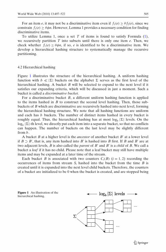
Figure 1 illustrates the structure of the hierarchical hashing. A uniform hashingfunction with b � |�| buckets on the alphabet � serves as the first level of thehierarchical hashing. A bucket B will be selected to expand to the next level if itsatisfies our expanding criteria, which will be discussed in just a moment. Such abucket is called a discriminative bucket.
For a discriminative bucket B, a different uniform hashing function is appliedto the items hashed in B to construct the second level hashing. Then, those sub-buckets of B which are discriminative are recursively hashed into next level, formingthe hierarchical hashing structure. We note that all hashing functions are uniformand each has b buckets. The number of distinct items hashed in every bucket isroughly equal. Thus, the hierarchical hashing has at most logb |�| levels. On thelogb |�|-th level, we directly put each item into a separate bucket, so that no conflictscan happen. The number of buckets on the last level may be slightly differentfrom b .
A bucket B at a higher level is the ancestor of another bucket B′ at a lower levelif B ⊃ B′, that is, any item hashed into B′ is hashed into B first. If B and B′ are attwo adjacent levels, B is also called the parent of B′ and B′ is a child of B. We call abucket a leaf if it has no child. Please note that a leaf bucket may still have multipleitems and may be expanded at a later time of the stream.
Each bucket B is associated with two counters Ci(B) (i = 1, 2) recording theoccurrences of items from stream Si hashed into the bucket from the time B iscreated until it is expanded into the next level child buckets. Therefore, the countersof a bucket are initialized to be 0 when the bucket is created, and are stopped being
Figure 1 An illustration of thehierarchical hashing.
506 World Wide Web (2010) 13:497–522
updated once the bucket is expanded. For a leaf bucket B, we can bound the sum ofthe frequencies of all items in B as
Ci(B) ≤∑
e∈B
fi(e) ≤ Ci(B) +∑
B′∈Anc(B)
Ci(B′),
where Anc(B) is the set of all ancestor buckets of B.To process a new item from stream Si, the new item is hashed all the way down to
the currently lowest level of the hierarchical hashing into the corresponding bucketB. The counter Ci(B) is incremented. We note again that the counters of the ancestorbuckets of B are not incremented. Only the bucket on the lowest level is updated.
Now, we present the expanding criteria that guides the hierarchical hashing to finddiscriminative items.
Lemma 2 (Discriminative buckets) Given a bucket B, let Anc(B) be the set ofancestor buckets of B. If
C1(B) ≥ θ(C2(B) +∑
B′∈Anc(B)
C2(B′)), (2)
then B contains at least one item e such that f1(e) ≥ θ f2(e).
Proof For all items e hashed into B,∑
e∈B
f1(e) ≥ C1(B),
and, due to the construction of the hierarchical hashing,∑
e∈B
f2(e) ≤ C2(B) +∑
B′∈Anc(B)
C2(B′).
Then,∑
e∈B
f1(e) ≥ θ∑
e∈B
f2(e).
By Lemma 1, this lemma follows immediately. ��
Based on Lemma 2, we call a bucket B a discriminative bucket if B satisfiesFormula (2) and C1(B) ≥ θφn. The condition C1(B) ≥ θφn is to make sure that Bis possible to contain frequent item in S1.
A bucket which used to be a discriminative bucket may be disqualified fromLemma 2 as the streams continue. Given a bucket B, if none of its child bucketsis discriminative at this moment, we delete all its child buckets and sum up theircounters to B. In detail, let Chi(B) denote the set of child buckets of B. The counterCi(B) (i = 1, 2) of B is increased by
∑B′∈Chi(B) Ci(B′). We note that the deleting
procedure is always conducted bottom-up from the lowest level.At the end, for an item e at the logb |�|-th level discriminative bucket, if f1(e) ≥
θφn, then, it is a discriminative item. By reporting all such items, the hash-basedmethod has 100% precision.
A bucket that does not satisfy Formula (2) is still possible to contain discriminativeitems. To boost the recall, we adopt the common methedology of applying multiple
World Wide Web (2010) 13:497–522 507
independent hierarchical hashings to process the streams. The number of hierarchicalhashing is determined empirically.
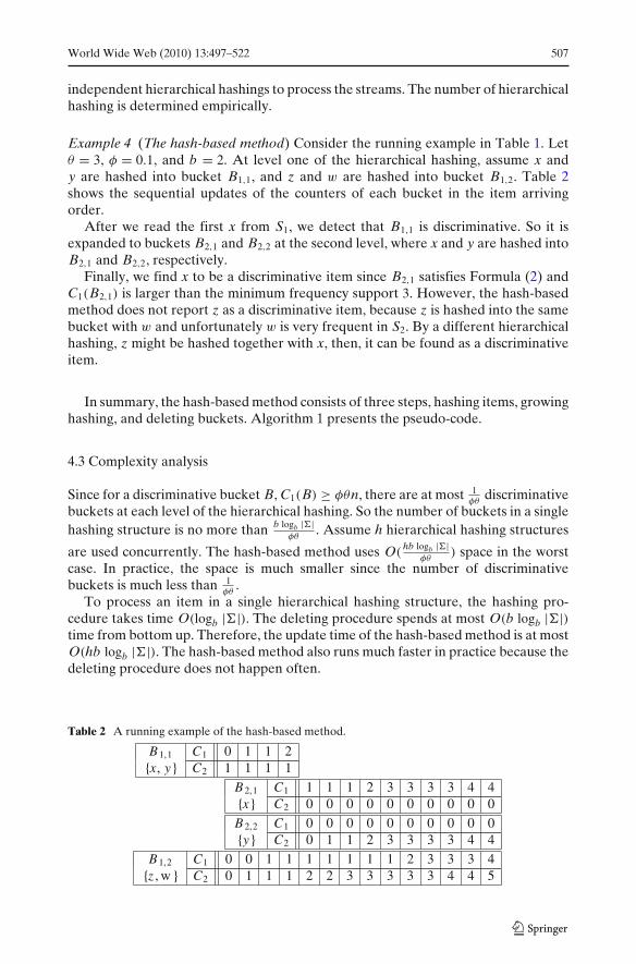
Example 4 (The hash-based method) Consider the running example in Table 1. Letθ = 3, φ = 0.1, and b = 2. At level one of the hierarchical hashing, assume x andy are hashed into bucket B1,1, and z and w are hashed into bucket B1,2. Table 2shows the sequential updates of the counters of each bucket in the item arrivingorder.
After we read the first x from S1, we detect that B1,1 is discriminative. So it isexpanded to buckets B2,1 and B2,2 at the second level, where x and y are hashed intoB2,1 and B2,2, respectively.
Finally, we find x to be a discriminative item since B2,1 satisfies Formula (2) andC1(B2,1) is larger than the minimum frequency support 3. However, the hash-basedmethod does not report z as a discriminative item, because z is hashed into the samebucket with w and unfortunately w is very frequent in S2. By a different hierarchicalhashing, z might be hashed together with x, then, it can be found as a discriminativeitem.
In summary, the hash-based method consists of three steps, hashing items, growinghashing, and deleting buckets. Algorithm 1 presents the pseudo-code.
4.3 Complexity analysis
Since for a discriminative bucket B, C1(B) ≥ φθn, there are at most 1φθ
discriminativebuckets at each level of the hierarchical hashing. So the number of buckets in a singlehashing structure is no more than b logb |�|
φθ. Assume h hierarchical hashing structures
are used concurrently. The hash-based method uses O(hb logb |�|
φθ) space in the worst
case. In practice, the space is much smaller since the number of discriminativebuckets is much less than 1
φθ.
To process an item in a single hierarchical hashing structure, the hashing pro-cedure takes time O(logb |�|). The deleting procedure spends at most O(b logb |�|)time from bottom up. Therefore, the update time of the hash-based method is at mostO(hb logb |�|). The hash-based method also runs much faster in practice because thedeleting procedure does not happen often.
Table 2 A running example of the hash-based method.
B 1,1 C1 0 1 1 2{x, y} C2 1 1 1 1
B 2,1 C1 1 1 1 2 3 3 3 3 4 4{x} C2 0 0 0 0 0 0 0 0 0 0
B 2,2 C1 0 0 0 0 0 0 0 0 0 0{y} C2 0 1 1 2 3 3 3 3 4 4
B 1,2 C1 0 0 1 1 1 1 1 1 1 2 3 3 3 4{z , w} C2 0 1 1 1 2 2 3 3 3 3 3 4 4 5
508 World Wide Web (2010) 13:497–522
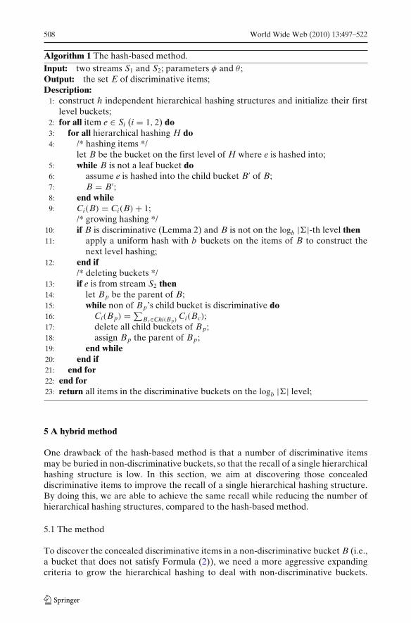
Algorithm 1 The hash-based method.Input: two streams S1 and S2; parameters φ and θ ;Output: the set E of discriminative items;Description:
1: construct h independent hierarchical hashing structures and initialize their firstlevel buckets;
2: for all item e ∈ Si (i = 1, 2) do3: for all hierarchical hashing H do4: /* hashing items */
let B be the bucket on the first level of H where e is hashed into;5: while B is not a leaf bucket do6: assume e is hashed into the child bucket B′ of B;7: B = B′;8: end while9: Ci(B) = Ci(B) + 1;
/* growing hashing */10: if B is discriminative (Lemma 2) and B is not on the logb |�|-th level then11: apply a uniform hash with b buckets on the items of B to construct the
next level hashing;12: end if
/* deleting buckets */13: if e is from stream S2 then14: let Bp be the parent of B;15: while non of Bp’s child bucket is discriminative do16: Ci(Bp) = ∑
Bc∈Chi(Bp) Ci(Bc);17: delete all child buckets of Bp;18: assign Bp the parent of Bp;19: end while20: end if21: end for22: end for23: return all items in the discriminative buckets on the logb |�| level;
5 A hybrid method
One drawback of the hash-based method is that a number of discriminative itemsmay be buried in non-discriminative buckets, so that the recall of a single hierarchicalhashing structure is low. In this section, we aim at discovering those concealeddiscriminative items to improve the recall of a single hierarchical hashing structure.By doing this, we are able to achieve the same recall while reducing the number ofhierarchical hashing structures, compared to the hash-based method.
5.1 The method
To discover the concealed discriminative items in a non-discriminative bucket B (i.e.,a bucket that does not satisfy Formula (2)), we need a more aggressive expandingcriteria to grow the hierarchical hashing to deal with non-discriminative buckets.

World Wide Web (2010) 13:497–522 509
Given a bucket, the items hashed into this bucket can be viewed as the sub-streams ofstreams S1 and S2, respectively. We build a space-saving summary on the sub-streamof S1 flowing through B. Thus, by this hybrid structure, we can capture items in Bwhich are frequent in S1. Then, by expanding B, we have a good chance to discoverdiscriminative items hidden in the non-discriminative bucket. Figure 2 illustrates theidea.
To be concrete, for each leaf bucket B, the hybrid method maintains a space-saving summary with k � |�|
b counters for items from S1 hashed into B. When B isselected to be expanded to the next level in the hashing growing phase, the countersof an item e ∈ B are forwarded to the corresponding child bucket of B where e ishashed into. Therefore, the space-saving summaries are only kept in leaf buckets.Any intermediate bucket does not keep such a summary. For an item e kept in thesummary of S1, in addition to its counter (e, c1(e), ε1(e)) of S1, we maintain anothercounter c2(e) to record the number of occurrences of e in S2 once it is recorded bythe summary of S1. By doing this, inequality c1(e) − ε1(e) ≤ f1(e) ≤ c1(e) still holds.
Using the space-saving summary, we handle discriminative buckets in a slightlydifferent way from the process in the hash-based method. For a bucket B, accordingto the space-saving algorithm introduced in Section 3.1, the k counters are initiallyfilled with the first k distinct items coming into B. In the hash-based method, a bucketB is expanded immediately once it is found to be discriminative. However, the kcounters of B already record the top-k most frequent items in B. It is not necessaryto expand B if the k counters are not all occupied. Therefore, we delay expanding adiscriminative bucket B until all k counters are used. In the process of expanding adiscriminative bucket, the existing counters are simply forwarded to its child buckets.
To handle non-discriminative buckets, in the cases where all k counters of a bucketB are used and B has not been found discriminative at the moment, we adopt amore aggressive expanding criteria. When a new item comes in B and it is differentfrom the k items in the summary, let e be the item with the minimum estimatedfrequency in S1 among the k items. We expand B to the next level if c1(e) − ε1(e) ≥max{φθn, μ}. Here, μ is a controlling parameter which is set to
√θ empirically. The
rationale behind this expanding criteria is that the k items kept in the summary havehigh possibility to be discriminative items, as they are frequent in S1.
Finally, to report discriminative items, we check every leaf bucket B in thehierarchical hashing structure. For each counter (e, c1(e), ε(e)) kept in B, we reporte as a discriminative item if c1(e)−ε(e)
c2(e)≥ θ . Although f1(e) ≥ c1(e) − ε(e), we cannot
guarantee that f2(e) ≤ c2(e), thus R(e) ≥ θ is not assured. However, the recall is
Figure 2 An illustration of thehybrid method.

510 World Wide Web (2010) 13:497–522
improved. Essentially, the hybrid method trades precision for recall. Our experi-ments in Section 6 verify that this trade-off is beneficial.
In the same way as the hash-based method, multiple hierarchical hashing struc-tures can be applied.
Example 5 (The hybrid method) For the running example in Table 1, the hash-basedmethod shown in Example 4 cannot find z as a discriminate item, since z is concealedby the effect of w. To tackle this problem, the hybrid method runs a space savingalgorithm on S1 with 1 counter. Then, it will find that z is frequent in S1 and expandbucket B1,2. At the end, the space-saving counter of z is (z, 4, 1) and the additionalcounter of z on stream S2 is c2(z) = 1. Thus, z is found to be discriminative.
5.2 Complexity analysis
In a single hierarchical hashing, to store the space-saving summaries, the hybridmethod requires at most O( bk
φθ) space more than the hash-based method, since there
are no more than O( bφθ
) leaf buckets. So the space complexity of the hybrid methodis
O(
hb logb |�|φθ
)+ O
(hbkφθ
)= O
(hb(logb |�| + k)
φθ
),
which is the same as the hash-based method. However, to achieve the same recall,the hybrid method reduces the number of hierarchical hashing needed. Therefore,the hybrid method is expected to outperform the hash-based method in terms ofspace usage.
The hybrid method needs to update both the hierarchical hashing and the space-saving summaries. With a heap implementation for the space-saving summaries,its time complexity is O(h(b logb |�| + log k)), and O(hb logb |�|) with the Stream-Summary data structure [30].
6 Empirical studies
We conducted experiments on real and synthetic data sets to evaluate the accuracyand efficiency of our three methods,1 the frequent item based method (FE), thehash-based method (HA), and the hybrid method (HY). The space-saving algorithmused in FE and HY was implemented using heap rather than the Stream-Summarystructure. The performance of our algorithms is not sensitivc to the minimum supportthreshold φ. So we set φ = 10−6 and does not change it in the experiments. For HAand HY, the hash fanout b is set to 32 all the time, and the number of counters usedin each bucket in HY is k = 5. The hash functions we use are pairwisely independentand implemented by the method stated in [8].
All methods were implemented in C++ and compiled by Microsoft Visual Studio2008. Experiments were conducted on a desktop computer with an Intel Core 2 DuoE8400 3GHz CPU and 4GB main memory running 64bit Microsoft Windows XP.
1The source code of the three methods can be downloaded at http://www.cs.sfu.ca/∼bjiang/personal/discriminative_item_code.zip.

World Wide Web (2010) 13:497–522 511
6.1 Synthetic data
We generated two streams in Zipfian distribution with skewness factor s varyingfrom 0.8 to 2. The size of each stream is 1,000,000 drawn from the alphabet �
whose size is 220 ≈ 1,000,000. We also ensure that there are a set of frequentitems in S1 also being frequent in S2, so that the set of discriminative items is nottrivially equivalent to the set of frequent items in S1. To do this, we select itemswith frequencies over 100 from S1 and randomly choose 25% of them so that theirfrequencies in S2 also exceeding 100. By default, the ratio parameter θ = 500, theskewness factor s = 1, and the number of hashes are 35 and 18 for HA and HY,
0 5000
10000 15000 20000 25000 30000 35000 40000
200 300 400 500 600 700 800 900 1000
Spa
ce(K
B)
FE HA HY
(a) Ratio θ .
0 5000
10000 15000 20000 25000 30000 35000 40000
0.8 1 1.2 1.4 1.6 1.8 2
Spa
ce(K
B)
FE HA HY
(b) Skewness factor s.
0 5000
10000 15000 20000 25000 30000 35000 40000
10 20 30 40 50 60
Spa
ce(K
B)
FE HA HY
(c) # of hashes h.
0 5000
10000 15000 20000 25000 30000 35000 40000
213 214 215 216 217 218
Spa
ce(K
B)
FE HA HY
(d) # of distinct items.
(e) n2n1
.
0 5000
10000 15000 20000 25000 30000 35000 40000 45000 50000
0.2 0.4
0.6 0.8
1 2 4 6 8 10
Spa
ce(K
B)
FE HA HY
Figure 3 Space on synthetic data sets.
512 World Wide Web (2010) 13:497–522
respectively, which are selected from our experiment results to balance accuracy andefficiency.
We conduct experiments to test the efficiency and accuracy of our three methodswith respect to the ratio parameter θ , the skewness factor s, the number of hashes h,the number of distinct items in the two streams, and the value of n2
n1.
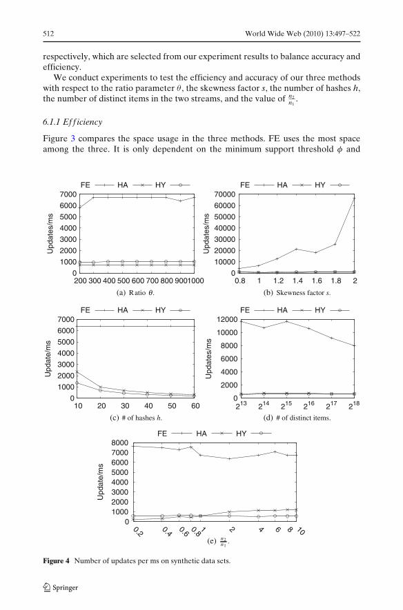
6.1.1 Ef f iciency
Figure 3 compares the space usage in the three methods. FE uses the most spaceamong the three. It is only dependent on the minimum support threshold φ and
0
1000
2000
3000
4000
5000
6000
7000
200 300 400 500 600 700 800 900 1000
Upd
ates
/ms
FE HA HY
(a) Ratio θ .
0
10000
20000
30000
40000
50000
60000
70000
0.8 1 1.2 1.4 1.6 1.8 2
Upd
ates
/ms
FE HA HY
(b) Skewness factor s.
0
1000
2000
3000
4000
5000
6000
7000
10 20 30 40 50 60
Upd
ate/
ms
FE HA HY
(c) # of hashes h.
0
2000
4000
6000
8000
10000
12000
213 214 215 216 217 218
Upd
ates
/ms
FE HA HY
(d) # of distinct items.
Upd
ate/
ms
(e) n2n1
.
0 1000 2000 3000 4000 5000 6000 7000 8000
0.2 0.4
0.6 0.8
1 2 4 6 8 10
FE HA HY
Figure 4 Number of updates per ms on synthetic data sets.
World Wide Web (2010) 13:497–522 513
invariant to the ratio parameter θ , the skewness factor s, the number of distinct items,and n2
n1.
HA uses only about 15 space of FE. Although the space complexity of HA is
O(hb logb |�|
φθ), Figure 3a shows that its space usage is not sensible to θ , because the
number of discriminative buckets is far less than 1φθ
. We also see that the spaceusage of HA is small on data sets of large skewness factors, where the number ofdiscriminative items is small. The space usage of HA increases linearly with respectto the number of hierarchical hashing. It also increases with respect to the number of
90
92
94
96
98
100
200 300 400 500 600 700 800 900 1000
Pre
cisi
on(%
)
FE HA HY
(a) Ratio θ .
90
92
94
96
98
100
0.8 1 1.2 1.4 1.6 1.8 2
Pre
cisi
on(%
)
FE HA HY
(b) Skewness factor s.
90
92
94
96
98
100
10 20 30 40 50 60
Pre
cisi
on(%
)
FE HA HY
(c) # of hashes h.
60 65 70 75 80 85 90 95
100
213 214 215 216 217 218
Pre
cisi
on(%
)
FE HA HY
(d) # of distinct items.
(e) n2n1
.
90
92
94
96
98
100
0.2 0.4
0.6 0.8
1 2 4 6 8 10
Pre
cisi
on(%
)
FE HA HY
Figure 5 Precision on synthetic data sets.
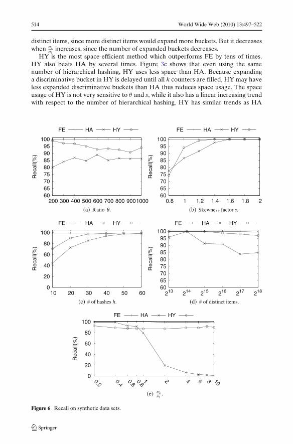
514 World Wide Web (2010) 13:497–522
distinct items, since more distinct items would expand more buckets. But it decreaseswhen n2
n1increases, since the number of expanded buckets decreases.
HY is the most space-efficient method which outperforms FE by tens of times.HY also beats HA by several times. Figure 3c shows that even using the samenumber of hierarchical hashing, HY uses less space than HA. Because expandinga discriminative bucket in HY is delayed until all k counters are filled, HY may haveless expanded discriminative buckets than HA thus reduces space usage. The spaceusage of HY is not very sensitive to θ and s, while it also has a linear increasing trendwith respect to the number of hierarchical hashing. HY has similar trends as HA
60 65 70 75 80 85 90 95
100
200 300 400 500 600 700 800 900 1000
Rec
all(%
)
FE HA HY
(a) Ratio θ .
60 65 70 75 80 85 90 95
100
0.8 1 1.2 1.4 1.6 1.8 2
Rec
all(%
)
FE HA HY
(b) Skewness factor s.
0
20
40
60
80
100
10 20 30 40 50 60
Rec
all(%
)
FE HA HY
(c) # of hashes h.
60 65 70 75 80 85 90 95
100
213 214 215 216 217 218
Rec
all(%
)
FE HA HY
(d) # of distinct items.
(e) n2n1
.
0
20
40
60
80
100
0.2 0.4
0.6 0.8
1 2 4 6 8 10
Rec
all(%
)
FE HA HY
Figure 6 Recall on synthetic data sets.

World Wide Web (2010) 13:497–522 515
Table 3 Topics in real datasets.
Data set Partition P1 Partition P2
Wikipedia Mathematics LawNewsgroups comp.graphics alt.atheism
comp.sys.ibm.pc.hardware rec.autoscomp.sys.mac.hardware rec.motorcyclescomp.os.ms-windows.misc rec.sport.baseballcomp.windows.x rec.sport.hockeymisc.forsale soc.religion.christiansci.crypt talk.politics.gunssci.electronics talk.politics.mideastsci.med talk.politics.miscsci.space talk.religion.misc
with respect to the number of distinct items and n2n1
, since they share the hierarchicalhashing structure.
The runtime is plotted in Figure 4. FE is the fastest method which can processmore than 6,000 items per millisecond. It can even handle more than 60,000 itemson data sets with skewness factor s = 2. In Figure 4b, we see that FE runs fasterin more skewed data sets. This is due to the heap implementation of the space-saving algorithm. We can expect a stable performance with the Stream-Summaryimplementation. FE also runs faster when the number of distinct items is small, sincein this case the summary does not change often.
HA and HY can support around 1,000 updates per millisecond. Figure 4a showsthat HY is slightly faster than HA, since HY uses less hierarchical hashing than HA.When using the same number of hashing, Figure 4c shows that HY is slower thanHA, as HY needs to maintain the space-saving summary.
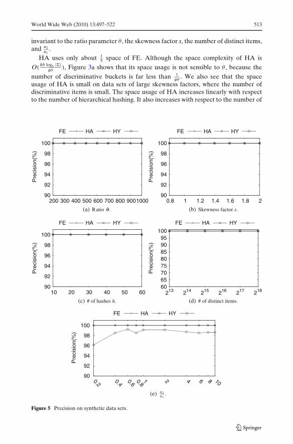
6.1.2 Accuracy
Figure 5 compares the precision of the three methods. As stated in Sections 3 and 4,FE and HA are guaranteed to have 100% precision. We see that the precision of HYis also close to 100%, and there is no clear trend related to the number of distinctitems and n2
n1.
In terms of recall, Figure 6 shows that FE has a recall of almost 100%. The recallsof HA and HY also increase to 100% as the skewness factor increases or usingmore hierarchical hashing. HY has a better recall than HA in most cases, even whenHY uses only a half number of hierarchical hashing. In Figure 6a, the recall of HAincreases slowly as θ increases, however, the recall of HY decreases. When θ is large,there are less expanded buckets since the expanding criteria of non-discriminativebuckets is controlled by the parameter μ = √
θ .Figure 6e shows that the recall of HA decreases dramatically as n2
n1increases over
1, since the number of expanded buckets decreases a lot because items from S2 flood
Table 4 Size of the real datasets in words.
Wikipedia Newsgroups
P1 P2 P1 P2
3,676,073 3,851,345 2,637,816 2,914,446

516 World Wide Web (2010) 13:497–522
Table 5 Top-5 mostdiscriminative words in theWikipedia data set.
Mathematics against law Law against mathematics
Words Ratio Words Ratio
Polynomial 855.55 Constitution 1,010.25Algebra 761.14 Jurisdiction 894.75Algebraic 703.65 Justice 480.38Geometry 679.17 Parliament 448.58Topology 645.50 Defendant 442.86
the buckets and make them difficult to expand. However, as a remedy, when n2n1
islarger than 1, we could duplicate every item from S1
n2n1
times it is observed it so thatS1 has similar size as S2. Then, we also scale θ to n2
n1θ correspondingly. So, the set of
discriminative does not change while HA can work well on the duplicated streams.
6.2 Real data
We use two real data sets, namely the Wikipedia data set and the 20 Newsgroupsdata set, obtained from http://en.wikipedia.org/ and http://people.csail.mit.edu/jrennie/20Newsgroups/, respectively. In the Wikipedia data set, we obtain 5,000articles on the topic of mathematics and 4,000 articles on the topic of law. Articleson the same topic are merged into one stream.
The 20 Newsgroups data set consists of 18, 846 newsgroup documents, partitionedevenly across 20 different newsgroups, each corresponding to a different topic shownin Table 3. We divide the 20 newsgroups into to 2 partitions as shown in Table 3, suchthat the topics in one partition are closely related to each other. Articles in the samepartition then are merged into a single stream.
For all articles, we only conduct stemming but do not filter out stopping words.Table 4 lists the size of the two partitions of each data set.
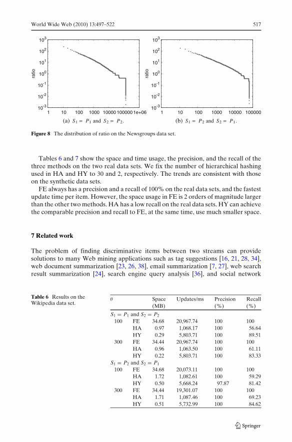
Table 5 lists the top-5 high ratio words in the Wikipedia data set, which match ourcommon intuition. Figures 7 and 8 show the ratio distribution of all terms on the tworeal data sets in log-log graph. We observe a power law distribution of the ratio. Thesharp tails are caused by the minimum support threshold φ.
10-3
10-2
10-1
100
101
102
103
1 10 100 1000 10000 100000
ratio
(a) S1 = P1 and S2 = P2.
10-3
10-2
10-1
100
101
102
103
1 10 100 1000 10000 100000
ratio
(b) S1 = P2 and S2 = P1.
Figure 7 The distribution of ratio on the Wikipedia data set.
World Wide Web (2010) 13:497–522 517
10-3
10-2
10-1
100
101
102
103
1 10 100 1000 10000 100000 1e+06
ratio
(a) S1 = P1 and S2 = P2.
10-3
10-2
10-1
100
101
102
103
1 10 100 1000 10000 100000
ratio
(b) S1 = P2 and S2 = P1.
Figure 8 The distribution of ratio on the Newsgroups data set.
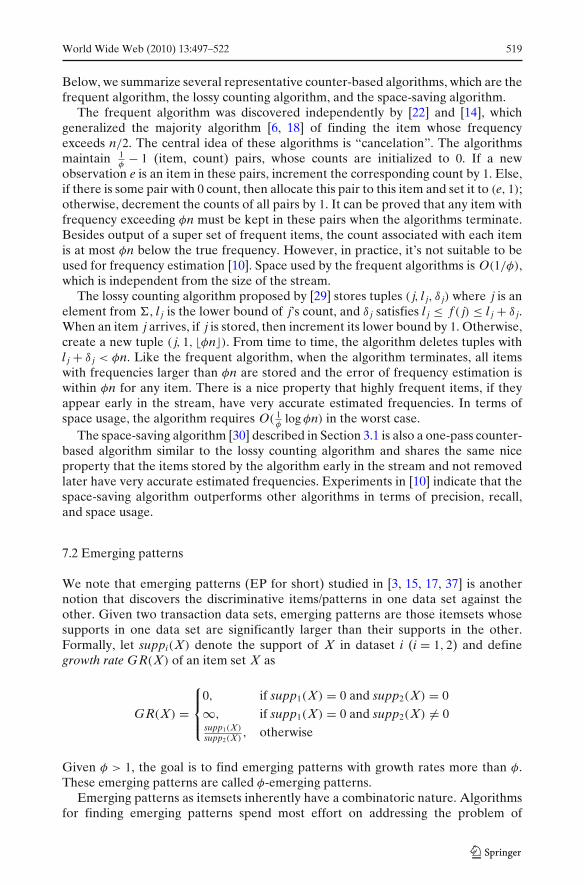
Tables 6 and 7 show the space and time usage, the precision, and the recall of thethree methods on the two real data sets. We fix the number of hierarchical hashingused in HA and HY to 30 and 2, respectively. The trends are consistent with thoseon the synthetic data sets.
FE always has a precision and a recall of 100% on the real data sets, and the fastestupdate time per item. However, the space usage in FE is 2 orders of magnitude largerthan the other two methods. HA has a low recall on the real data sets. HY can achievethe comparable precision and recall to FE, at the same time, use much smaller space.
7 Related work
The problem of finding discriminative items between two streams can providesolutions to many Web mining applications such as tag suggestions [16, 21, 28, 34],web document summarization [23, 26, 38], email summarization [7, 27], web searchresult summarization [24], search engine query analysis [36], and social network
Table 6 Results on theWikipedia data set.
θ Space Updates/ms Precision Recall(MB) (%) (%)
S1 = P1 and S2 = P2
100 FE 34.68 20,967.74 100 100HA 0.97 1,068.17 100 56.64HY 0.29 5,803.71 100 89.51
300 FE 34.44 20,967.74 100 100HA 0.96 1,063.50 100 61.11HY 0.22 5,803.71 100 83.33
S1 = P2 and S2 = P1
100 FE 34.68 20,073.11 100 100HA 1.72 1,082.61 100 59.29HY 0.50 5,668.24 97.87 81.42
300 FE 34.44 19,301.07 100 100HA 1.71 1,087.46 100 69.23HY 0.51 5,732.99 100 84.62

518 World Wide Web (2010) 13:497–522
Table 7 Results on theNewsgroups data set.
θ Space Updates/ms Precision Recall(MB) (%) (%)
S1 = P1 and S2 = P2
100 FE 34.68 17,795.71 100 100HA 3.24 981.49 100 59.57HY 0.65 5,470.21 91.67 93.62
200 FE 34.50 16,927.63 100 100HA 3.23 973.57 100 68.75HY 0.36 5,552.26 93.75 93.75
S1 = P2 and S2 = P1
100 FE 34.68 16,876.18 100 100HA 1.12 984.27 100 33.33HY 0.48 5,228.12 82.35 93.33
200 FE 34.50 16,140.30 100 100HA 1.11 989.71 100 42.86HY 0.30 5,464.82 77.78 100
analysis [32, 35]. An essential issue inherent in those applications is to find discrim-inative tags or keywords that can distinguish the target object from many others.Statistically, we model such discrimination in frequency ratio. Due to the largeamount of data arriving or being generated in high speed on the Web, the streamingmodel is appropriate.
Discriminative items are highly related to frequent items in data streams andemerging patterns in pattern mining. We review the studies on mining frequent itemsin data streams and mining emerging patterns in Section 7.1 and 7.2, respectively.
7.1 Finding frequent items in data streams
The problem of finding frequent items is extensively studied in data stream com-munity since 1980s due to its intuitive interest and importance. In the literature,there are various formulations of this problem, including finding top-k most frequentitems [9, 30, 31], finding all frequent items with respect to a user-specified frequencythreshold [2, 22, 25], finding frequent items over sliding windows [2, 13, 25, 31],and so on. Among all these formulations, the problem of finding all frequent itemswith respect to a user-specified frequency threshold is the one most relevant to ourproblem. We review the major algorithms of this problem in detail.
Formally, given a stream S of length n and a threshold φ, the goal is to return aset of items E so that for each e ∈ E, the frequency f (e) ≥ φn. Unfortunately, anyonline algorithm that finds the exact set E must use �(|�| log n
|�| ) space in the worstcase [22], where � denotes the alphabet. To overcome this lower bound, the problemof finding ε-approximate frequent items [29, 30] is introduced. The goal is to find aset of items E where each item e ∈ E satisfies f (e) > (φ − ε)n.
Cormode and Hadjieleftheriou [10] compared several algorithms on this subject,and divided them into three classes, namely, counter-based algorithms [6, 14, 22,29, 30], quantile algorithms [20, 29], and randomized sketch algorithms [1, 11, 12].Besides finding frequent items, counter-based algorithms can also estimate theirfrequencies. We note that any counter-based algorithm can be plugged into theframework of our frequent item-based method for finding discriminative items.
World Wide Web (2010) 13:497–522 519
Below, we summarize several representative counter-based algorithms, which are thefrequent algorithm, the lossy counting algorithm, and the space-saving algorithm.
The frequent algorithm was discovered independently by [22] and [14], whichgeneralized the majority algorithm [6, 18] of finding the item whose frequencyexceeds n/2. The central idea of these algorithms is “cancelation”. The algorithmsmaintain 1
φ− 1 (item, count) pairs, whose counts are initialized to 0. If a new
observation e is an item in these pairs, increment the corresponding count by 1. Else,if there is some pair with 0 count, then allocate this pair to this item and set it to (e, 1);otherwise, decrement the counts of all pairs by 1. It can be proved that any item withfrequency exceeding φn must be kept in these pairs when the algorithms terminate.Besides output of a super set of frequent items, the count associated with each itemis at most φn below the true frequency. However, in practice, it’s not suitable to beused for frequency estimation [10]. Space used by the frequent algorithms is O(1/φ),which is independent from the size of the stream.
The lossy counting algorithm proposed by [29] stores tuples ( j, l j, δ j) where j is anelement from �, l j is the lower bound of j’s count, and δ j satisfies l j ≤ f ( j) ≤ l j + δ j.When an item j arrives, if j is stored, then increment its lower bound by 1. Otherwise,create a new tuple ( j, 1, �φn�). From time to time, the algorithm deletes tuples withl j + δ j < φn. Like the frequent algorithm, when the algorithm terminates, all itemswith frequencies larger than φn are stored and the error of frequency estimation iswithin φn for any item. There is a nice property that highly frequent items, if theyappear early in the stream, have very accurate estimated frequencies. In terms ofspace usage, the algorithm requires O( 1
φlog φn) in the worst case.
The space-saving algorithm [30] described in Section 3.1 is also a one-pass counter-based algorithm similar to the lossy counting algorithm and shares the same niceproperty that the items stored by the algorithm early in the stream and not removedlater have very accurate estimated frequencies. Experiments in [10] indicate that thespace-saving algorithm outperforms other algorithms in terms of precision, recall,and space usage.
7.2 Emerging patterns
We note that emerging patterns (EP for short) studied in [3, 15, 17, 37] is anothernotion that discovers the discriminative items/patterns in one data set against theother. Given two transaction data sets, emerging patterns are those itemsets whosesupports in one data set are significantly larger than their supports in the other.Formally, let suppi(X) denote the support of X in dataset i (i = 1, 2) and definegrowth rate GR(X) of an item set X as
GR(X) =
⎧⎪⎨
⎪⎩
0, if supp1(X) = 0 and supp2(X) = 0
∞, if supp1(X) = 0 and supp2(X) �= 0supp1(X)
supp2(X), otherwise
Given φ > 1, the goal is to find emerging patterns with growth rates more than φ.These emerging patterns are called φ-emerging patterns.
Emerging patterns as itemsets inherently have a combinatoric nature. Algorithmsfor finding emerging patterns spend most effort on addressing the problem of

520 World Wide Web (2010) 13:497–522
compactly representing emerging patterns and efficient manipulation of emergingpatterns to avoid enumerating all possible itemsets. Mining discriminative items doesnot need to deal with this issue. Furthermore, the problem of emerging patterns areconsidered in a static transaction database environment. We position our problem inthe data stream settings and focus on reducing memory space of use. To the best ofour knowledge, we are the first to study the problem of finding discriminative itemsbetween two data streams.
8 Conclusions
In this paper, motivated by a class of Web mining applications including taggingWeb objects, summarizing web documents, and analyzing search queries, we tacklethe problem of finding discriminative items between streams, which are frequent inone stream but infrequent in another. We prove a space lower bound of exactlyfinding all discriminative items and develop three heuristic algorithms that by onescan can achieve high precision and recall using sub-linear space and sub-linearprocessing time per item with respect to the size of the alphabet. The complexityof all algorithms are independent from the size of streams.
References
1. Alon, N., Matias, Y., Szegedy, M.: The space complexity of approximating the frequencymoments. In: Proceedings of the 28th Annual ACM Symposium on Theory of Computing(STOC’96), pp. 20–29 (1996)
2. Arasu, A., Manku, G.S.: Approximate counts and quantiles over sliding windows. In: Proceed-ings of 23th ACM SIGMOD Principles of Database Systems (PODS’04), pp. 286–296 (2004)
3. Bailey, J., Manoukian, T., Ramamohanarao, K.: Fast algorithms for mining emerging patterns.In: Proceedings of 6th European Conference on Principles and Practice of Knowledge Discoveryin Databases (PKDD’02), pp. 39–50 (2002)
4. Blei, D.M., Lafferty, J.D.: Dynamic topic models. In: Proceedings of the 23rd InternationalConference (ICML’06), ACM, ACM International Conference Proceeding Series, vol. 148,pp. 113–120 (2006)
5. Blei, D.M., Ng, A.Y., Jordan, M.I.: Latent dirichlet allocation. J. Mach. Learn. Res. 3, 993–1022(2003)
6. Boyer, R.S., Moore, J.S.: Mjrty: a fast majority vote algorithm. In: Automated Reasoning: Essaysin Honor of Woody Bledsoe, pp. 105–118 (1991)
7. Carenini, G., Ng, R.T., Zhou, X.: Summarizing email conversations with clue words. In: Proceed-ings of 16th International World Wide Web Conference (WWW’07), pp. 91–100 (2007)
8. Carter, L., Wegman, M.N.: Universal classes of hash functions (extended abstract). In: Proceed-ings of the 9th Annual ACM Symposium on Theory of Computing (STOC’77), pp. 106–112(1977)
9. Charikar, M., Chen, K., Farach-Colton, M.: Finding frequent items in data streams. In: Proceed-ings of 29th International Colloquium on Automata, Languages and Programming (ICALP’02),pp. 693–703 (2002)
10. Cormode, G., Hadjieleftheriou, M.: Finding frequent items in data streams. In: Proceedings ofthe VLDB Endowment (PVLDB’08), vol. 1, no. 2, pp. 1530–1541 (2008)
11. Cormode, G., Muthukrishnan, S.: What’s new: finding significant differences in network datastreams. In: Proceedings of 23rd Annual Joint Conference of the IEEE Computer and Commu-nications Societies (INFOCOM’04) (2004)
12. Cormode, G., Muthukrishnan, S.: An improved data stream summary: the count-min sketch andits applications. J. Algorithms 55(1), 58–75 (2005)

World Wide Web (2010) 13:497–522 521
13. Datar, M., Gionis, A., Indyk, P., Motwani, R.: Maintaining stream statistics over sliding win-dows (extended abstract). In: Proceedings of 13th Annual ACM-SIAM Symposium on DiscreteAlgorithms (SODA’02), pp. 635–644 (2002)
14. Demaine, E.D., López-Ortiz, A., Munro, J.I.: Frequency estimation of internet packet streamswith limited space. In: Proceedings of 10th European Symposium on Algorithms (ESA’02),pp. 348–360 (2002)
15. Dong, G., Li, J.: Efficient mining of emerging patterns: discovering trends and differences. In:Proceedings of 5th ACM SIGKDD International Conference on Knowledge Discovery and DataMining (SIGKDD’99), pp. 43–52 (1999)
16. Dubinko, M., Kumar, R., Magnani, J., Novak, J., Raghavan, P., Tomkins, A.: Visualizing tagsover time. In: Proceedings of 15th International World Wide Web Conference (WWW’06),pp. 193–202 (2006)
17. Fan, H., Ramamohanarao, K.: An efficient single-scan algorithm for mining essential jumpingemerging patterns for classification. In: Proceedings of 6th Pacific-Asia Conference on Knowl-edge Discovery and Data Mining (PAKDD’02), pp. 456–462 (2002)
18. Fischer, M.J., Salzberg, S.L.: Finding a majority among n votes. J. Algorithms 3, 376–379 (1982)19. Ganguly, S.: Lower bounds on frequency estimation of data streams. In: Proceedings of 3rd
International Computer Science Symposium in Russia (CSR’08). Lecture Notes in ComputerScience, vol. 5010, pp. 204–215. Springer (2008)
20. Greenwald, M., Khanna, S.: Space-efficient online computation of quantile summaries. In:Proceedings of the 2001 ACM SIGMOD International Conference on Management of Data(SIGMOD’01), pp. 58–66 (2001)
21. Halpin, H., Robu, V., Shepherd, H.: The complex dynamics of collaborative tagging. In: Proceed-ings of 16th International World Wide Web Conference (WWW’07), pp. 211–220 (2007)
22. Karp, R.M., Shenker, S., Papadimitriou, C.H.: A simple algorithm for finding frequent elementsin streams and bags. ACM Trans. Database Syst. 28, 51–55 (2003)
23. Khy, S., Ishikawa, Y., Kitagawa, H.: A novelty-based clustering method for on-line documents.World Wide Web 11(1), 1–37 (2008)
24. Kuo, B.Y.L., Hentrich, T., Good, B.M., Wilkinson, M.D.: Tag clouds for summarizing websearch results. In: Proceedings of 16th International World Wide Web Conference (WWW’07),pp. 1203–1204 (2007)
25. Lee, L.K., Ting, H.F.: A simpler and more efficient deterministic scheme for finding frequentitems over sliding windows. In: Proceedings of 25th ACM SIGMOD Principles of DatabaseSystems (PODS’06), pp. 290–297 (2006)
26. Li, L., Zhou, K., Xue, G.R., Zha, H., Yu, Y.: Enhancing diversity, coverage and balance forsummarization through structure learning. In: Proceedings of 18th International World WideWeb Conference (WWW’09), pp. 71–80 (2009)
27. Li, W., Zhong, N., Yao, Y., Liu, J.: An operable email based intelligent personal assistant. WorldWide Web 12(2), 125–147 (2009)
28. Liu, D., Hua, X.S., Yang, L., Wang, M., Zhang, H.J.: Tag ranking. In: Proceedings of 18thInternational World Wide Web Conference (WWW’09), pp. 351–360 (2009)
29. Manku, G.S., Motwani, R.: Approximate frequency counts over data streams. In: Proceedingsof 28th International Conference on Very Large Data Bases (VLDB’02), pp. 346–357. MorganKaufmann (2002)
30. Metwally, A., Agrawal, D., Abbadi, A.E.: Efficient computation of frequent and top-k ele-ments in data streams. In: Proceedings of 10th International Conference on Database Theory(ICDT’05), pp. 398–412 (2005)
31. Pingda, S., Huahui, C.: A new method to find top k items in data streams at arbitrary time gran-ularities. In: Proceedings of 2008 International Conference on Computer Science and SoftwareEngineering (CSSE’08), vol. 4, pp. 267–270 (2008)
32. Sen, S., Vig, J., Riedl, J.: Tagommenders: connecting users to items through tags. In: Proceedingsof 18th International World Wide Web Conference (WWW’09), pp. 671–680 (2009)
33. Steyvers, M., Griffiths, T.: Probabilistic Topic Models. Lawrence Erlbaum Associates (2007)34. Wu, L., Yang, L., Yu, N., Hua, X.S.: Learning to tag. In: Proceedings of 18th International World
Wide Web Conference (WWW’09), pp. 361–370 (2009)35. Wu, X., Zhang, L., Yu, Y.: Exploring social annotations for the semantic web. In: Proceedings of
15th International World Wide Web Conference (WWW’06), pp. 417–426 (2006)36. Yi, J., Maghoul, F., Pedersen, J.O.: Deciphering mobile search patterns: a study of yahoo! mobile
search queries. In: Proceedings of 17th International World Wide Web Conference (WWW’08),pp. 257–266 (2008)

522 World Wide Web (2010) 13:497–522
37. Zhang, X., Dong, G., Ramamohanarao, K.: Exploring constraints to efficiently mine emergingpatterns from large high-dimensional datasets. In: Proceedings of 6th ACM SIGKDD Inter-national Conference on Knowledge Discovery and Data Mining (SIGKDD’00), pp. 310–314(2000)
38. Zhu, J., Wang, C., He, X., Bu, J., Chen, C., Shang, S., Qu, M., Lu, G.: Tag-oriented documentsummarization. In: Proceedings of 18th International World Wide Web Conference (WWW’09),pp. 1195–1196 (2009)