Minimum-Loss Network Reconfiguration: A Minimum Spanning Tree Problem

Hamed Ahmadia,∗, José R. Martía

aDepartment of Electrical and Computer Engineering, The University of British Columbia, 2332 Main Mall, Vancouver, BC,Canada V6T 1Z4.

Abstract

Topological reconfiguration of power distribution systems can result in operational savings by reducing the

power losses in the network. In this paper, an efficient heuristic is proposed to find an initial solution for

the minimum-loss reconfiguration problem with small optimality gap. Providing an initial solution for a

mixed-integer programming (MIP) problem, known as “warm-start”, allows for a significant speed up in the

solution process. The network reconfiguration for loss reduction is mapped here into a problem of finding a

minimum spanning tree (MST) in a graph, for which there are a number of efficient algorithms developed

in the literature. The proposed method leads to very fast solutions (less than 1.4 s for systems up to

10476 nodes). For the test systems considered, the solution provided by the proposed method lies within a

relative optimality gap of about 2.2% with respect to the optimal solution. The existing MST algorithms

guarantee the scalability of the proposed routine for large-scale distribution systems. Sensitivity factors are

also employed to refine the solution to a smaller optimality gap.

Keywords: Power distribution systems, topological reconfiguration, minimum spanning tree.

1. Introduction

The tendency towards optimizing the utilization of the current infrastructure in power systems has been

significantly increased in the past decade. The costs and technical difficulties associated with building new

lines is a major motivation [1]. Also, reducing power losses has become a desirable objective for many

distribution companies (DISCOs). Distribution systems (DS) are the last stage of the electricity network

supplying energy to customers. Conventionally, DS’s have been operated in radial configuration due to the

simplicity of operating and protecting a radial system. Although not often, weakly-meshed configurations are

sometimes encountered. Despite their extended use, radial structures are relatively vulnerable in that they

have a single point of supply. Nonetheless, losing a single feeder within the whole of a DS is not potentially

a threat for the entire power system operation and, therefore, the radial structure is still usually preferred.

One of the important operational problems in DS is the topological reconfiguration for loss reduction, load

∗Corresponding authorEmail address: hameda@ece.ubc.ca (Hamed Ahmadi)

Preprint submitted to Sustainable Energy, Grids and Networks October 31, 2014

balancing, voltage profile improvement, etc. There are usually controllable switches in DS’s using which the

operator can alter system’s topology by performing opening/closing actions. Since the number of switches

are relatively high in practical systems, it is almost impossible for the operator to find the best topology

without an optimization study. Many algorithms for DS reconfiguration have been developed, e.g., [2]-[4]. In

these studies, the condition of radiality of the final network is normally imposed. This constraint, however,

is not easy to represent as a mathematical formula, which is also recognized in [5] and [6].

The term “radial” refers to a configuration that includes all the nodes but has no loops. A literature

review on this subject is provided in [5] and [6] which articulates the different approaches for imposing the

radiality constraint in a configuration optimization problem. In heuristic methods, the radiality constraint

is usually dealt with implicitly. Examples of heuristic methods used in the literature for network reconfigu-

ration are Genetic Algorithms [7] and [8], Harmony Search [9], Simulated Annealing [10], Artificial Neural

Networks [11], Plant Growth Simulation [12], Tabu Search [13], Particle Swarm Optimization [14], and Ant

Colony [15]. In direct mathematical models, on the other hand, there needs to be a mathematical formula-

tion for representing the radiality constraint. A few studies provide mathematical models for the radiality

constraint, such as [16]-[21].

The standard constraints in an optimal DS reconfiguration problem are power flow equations, nodal volt-

age limits, feeders ampacity limits, and radiality. Formulating this problem using the traditional power flow

equations leads to a mixed-integer nonlinear programming (MINLP) problem [22]. Solving large-scale MINLP

problems is not practically possible due to the tremendous amount of computations required. Therefore,

researchers have tried to tackle the problem using heuristic methods. The advantage of heuristic methods

is their low computational complexity while being unreliable and/or suboptimal. A sensible combination of

algorithms would be to use heuristics to find a good initial solution and then use this solution to initiate a

deterministic mathematical optimization, e.g., [20].

There are a few deterministic mathematical formulation of the network reconfiguration problem that are

in the form of a mixed-integer programming (MIP) problem. A mixed-integer conic programming formula-

tion is proposed in [18] for network reconfiguration. It takes over 0.5 h for the algorithm in [18] to find an

optimal/near-optimal solution for a network with 135 nodes. Network reconfiguration problem is formulated

as a second-order cone programming in [19]. This method takes hours to provide optimal solution for a

system with 880 nodes. A mixed-integer quadratically-constrained programming (MIQCP) formulation of

the reconfiguration problem is proposed in [20] which is based on a linear power flow algorithm developed in

[23]. The optimization problem in [20] takes about three minutes to solve the problem for a 135-node system.

A mixed-integer linear programming formulation for the reconfiguration problem is developed in [24] which

linearizes the current injections at each node as well as the quadratic terms in the objective function and

constraints. Although all the aforementioned deterministic approaches provide many advantages in terms

2

of flexibility of the formulation (e.g., for adding extra constraints, aiming at different objectives, knowledge

about the optimality gap at every iteration, etc.), they do not take advantage of a good initial solution to

start the MIP solver. Many commercial MIP solvers allow for a “warm- start”, i.e. starting from a known

solution, to speed up the search for the global optimum, e.g., CPLEX [25] and GUROBI [26].

In this paper, a fast method is sought which provides a suboptimal solution for the minimum-loss recon-

figuration problem with a small optimality gap. This can replace the first stage of the MIP solution process

that most of the commercial solvers have as a built-in routine. This routine searches for a feasible solution

using some general-purpose heuristic methods. Those heuristics, however, are relatively slow and often find

a solution with a large optimality gap. Providing a good initial solution to start with, the solution time can

be significantly reduced [25].

The problem of finding a radial topology for a DS with minimum losses can be interpreted as finding

a spanning tree in the network that also generates minimal losses. The minimum spanning tree (MST)

algorithm has been adopted in [27] to find a radial topology that minimizes the energy-not-supplied. In

order to assure radiality, different MST algorithms are utilized in [28] (Kruskal algorithm) and [29] (Prim

algorithm) within a Genetic Algorithm-based search. However, the only use of the MST algorithms in the

referred studies is to help finding a radial configuration, not to find the minimum losses.

In this paper, the problem of minimum-loss DS reconfiguration is mapped into a MST problem based on

some assumptions. The main assumption here, based on engineering knowledge, is that the meshed network

is a good solution (if not the best) for loss minimization when the radiality constraint is relaxed. The same

assumption has been made in [21] with a slight difference. In [21], it is assumed that the meshed network

generates the least possible losses, which may not be always true as shown in this paper. However, the dif-

ference between the losses in the meshed network and the best-possible network configuration is negligible,

as is also shown later in this paper. The second assumption in the present paper is that reconfiguring the

network in order to reduce the losses will implicitly improve the voltage profile. This assumption has been

previously validated in [4], and is also validated in this paper on various test systems. The voltage profile

can also be modified by adjusting capacitor banks, voltage regulators, and transformers tap positions, as is

done in [20], outside of the reconfiguration process.

Based on the assumptions mentioned in the previous paragraph, the problem of DS reconfiguration for

loss reduction is defined as “finding a spanning tree that imitates, as closely as possible, the same flow pattern

as the meshed network”. The idea of starting from a meshed network and opening switches sequentially has

been proposed in [4], called DISTOP. There are two main differences between DISTOP and the proposed

method in this paper. The first difference is that after every switching action, a new power flow solution

is required in DISTOP, while only one power flow solution is sufficient for the proposed algorithm in this

paper. The other difference is how the algorithms check whether a configuration is radial. It is stated in [4]

3

that the switches are opened one after another until the network becomes radial. However, it is not explicitly

explained how to check the radiality. In many cases, disconnecting a switch that carries the minimum current

leads to a disconnected network. It is not trivial to check if the network remains connected after opening

a particular switch. The proposed algorithm in this paper, on the other hand, is guaranteed to provide a

radial configuration.

The proposed heuristic method here has the advantage of using a fast and robust algorithm that also

finds a high-quality solution (with small optimality gap). The efficient MST algorithms developed in the

literature such as Kruskal [30] and Prim [31] algorithms can be employed to solve the formulated problem.

A refinement to the solution is done by sensitivity analysis around the neighborhood of the candidate tie

switches. In order to do that, line outage distribution factors (LODF) are derived based on the linear power

flow formulation in [23].

The rest of this paper is organized as follows. In Section 2, a brief background on graph theory and the

MST problem is presented. In Section 3, the DS reconfiguration problem is converted into a MST problem.

Section 4 presents the application of the proposed method to various test cases. The main findings of this

study are summarized in Section 5.

2. Background: Minimum Spanning Tree

A spanning tree is a subgraph of an undirected graph that contains all the vertices (i.e. it is connected)

and has no cycles (has no loops). The MST in a weighted undirected graph is the subgraph that is a spanning

tree, and the sum of its weights is the minimum possible. This problem is well-addressed in the literature

under the name “minimum spanning tree” (MST) and there are efficient algorithms such as Kruskal [30] and

Prim [31] to solve the problem. Besides, there are parallel algorithms to solve the MST problem even faster,

e.g., [32]. By negating the weights, the algorithms for MST will find the maximum spanning tree [33]. The

time complexity (the amount of time taken by the algorithm to run as a function of the network size) of

a version of Prim’s algorithm which is suitable for sparse graphs is O(e log v), which is similar to the time

complexity of Kruskal’s algorithm.

Prim’s algorithm is used in this paper to find the MST. There is basically no advantage of using Prim’s

algorithm over Kruskal’s, and one may choose the other. It is important to emphasize that these algorithms

provide the optimal solution to the MST problem. The structure of the Prim’s algorithm for a weighted

undirected graph G(V,E) with V vertices and E edges is summarized in the following steps.

1. Choose any vertex r in V to be the root node. Set Vt = {r} and Et = ∅.

2. Find an edge with the smallest weight such that one of its end points is in S and the other is in V \Vt.

Add this edge to Et and its new vertex to S.

4

Table 1: MST Search For The 14-Node Graph Using Prim’s Algorithm

Iteration 1 2 3 4 5 6 7

New Edge 1-6 1-2 1-11 6-7 2-3 7-10 11-13

New Vertex 6 2 11 7 3 10 13

Iteration 8 9 10 11 12 13

New Edge 13-14 3-9 2-4 11-12 12-8 4-5

New Vertex 14 9 4 12 8 5

12

3

4

5

6

7

89

10

11

12

13

14

0.07630.1108

0.1121

0.0743

0.0486

0.0234

0.0290

0.0597

0.0284

0.01270.0081

0.0298

0.0395

0.00640.0201

0.0254

(a) Weighted 16-node graph

12

3

4

5

6

7

89

10

11

12

13

14

(b) MST of the 16-node graph

Figure 1: The 16-node graph and its MST.

3. If V \Vt = ∅, then terminate. Otherwise, go back to Step 2.

Prim’s algorithm is applied to the 14-node graph shown in Fig. 1(a). The final spanning tree obtained

using the MST algorithm is shown in Fig. 1(b).

3. Distribution System Reconfiguration: A Minimum Spanning Tree Problem

In this section, the MST algorithm is applied, as a heuristic method, to the DS reconfiguration problem.

This problem aims at finding a radial topology which admits the minimum resistive losses. It is stated in

[21] that the minimum-loss network is achieved when all the switches are closed. This statement, however,

does not always hold. In order to show this the problem is solved without imposing the radiality constraint.

The results of these simulations obtained by the MIQCP method proposed in [20] are reported in Section 4.

The following assumptions are derived based on the engineering knowledge of DS and are used throughout

this paper. When all the tie-switches are closed, forming a weakly-meshed network, then

5

• the losses are close (if not exactly the same) to the losses of the best-possible configuration.

• the load is distributed between the feeders and a moderate balance (but not the best-possible) among

all the feeders is achieved.

• the voltage profile of the network is close to the best-possible voltage profile.

The validity of these assumptions is demonstrated through examples in Section 4. Note that loss reduc-

tion, load balancing between feeders, and voltage profile improvement are three different objectives and may

lead to different configurations. However, loss reduction implicitly improves the voltage profile, as was also

previously acknowledged in [4], and maintain a moderate balance between feeders, as was also recognized in

[34].

It is shown here, mathematically, that the loss minimization is in alignment with voltage profile improve-

ment. The total losses in a DS, as derived in [20], are obtained as:

Ploss =∑

(i,j)∈SL

Gij

[(V re

i − V rej )2 + (V im

i − V imj )2

](1)

where G is the branch conductance; SL is the set of all the branches; V re and V im are the real and imaginary

pars of the nodal voltages. The voltage at the substation node is usually considered to be a known quantity.

Normally, the following values are assumed for the substation voltage: V res = 1 and V im

s = 0. Recall the fact

from [20] that the nodal voltage magnitudes are mainly governed by their real parts, i.e. V re. Minimizing

(1) can be translated into minimizing the differences between the real parts of the nodal voltages. Since one

of the voltages, i.e. V res , is already fixed at 1 p.u., the other nodal voltages are also pushed to stay close

to 1 p.u. to minimize the objective in (1). This argument reveals the fact that minimizing losses implicitly

improves the voltage profile of a distribution network.

Let us look at a meshed DS as a weighted undirected graph, where the negative of the current magnitudes

are taken as the weights. The problem of finding a tree for the meshed network that closely imitates it can

be converted into a MST problem. The MST algorithm tries to keep the branches with the largest current

magnitudes (note the negative sign) and open the branches with the least currents to form a tree. For

example, take the 14-node graph shown in Fig. 1(a), which is the 14-node system of [2], with the current

magnitudes shown for each branch. Figure 1(b) shows that the branches with the least currents, i.e. 5-14,

6-8, and 7-9 are open in the MST solution.

Although the above discussed method appears reasonable, network constraints, such as nodal voltage

limits and feeder ampacities have not been explicitly considered. However, it is shown in Section 4 that

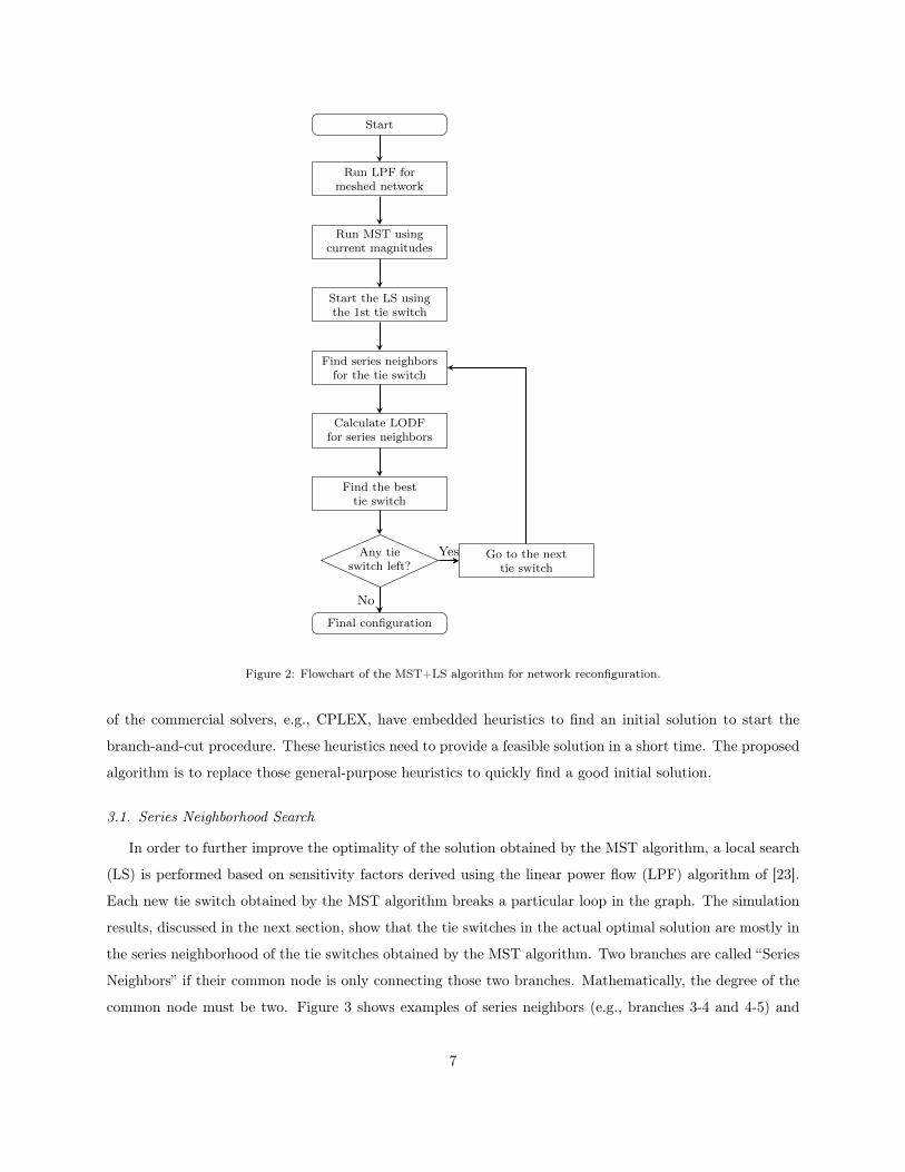
the system operational constraints are implicitly satisfied in the final results. The flowchart of the proposed

algorithm is shown in Fig. 2. Recall that the MST algorithm proposed here is meant to quickly find a good

initial solution to be used in a direct mathematical approach, such as the MIQCP problem in [20]. Most

6

Start

Run LPF formeshed network

Run MST usingcurrent magnitudes

Start the LS usingthe 1st tie switch

Find series neighborsfor the tie switch

Calculate LODFfor series neighbors

Find the besttie switch

Any tieswitch left?

Go to the nexttie switch

Final configuration

No

Yes

Figure 2: Flowchart of the MST+LS algorithm for network reconfiguration.

of the commercial solvers, e.g., CPLEX, have embedded heuristics to find an initial solution to start the

branch-and-cut procedure. These heuristics need to provide a feasible solution in a short time. The proposed

algorithm is to replace those general-purpose heuristics to quickly find a good initial solution.

3.1. Series Neighborhood Search

In order to further improve the optimality of the solution obtained by the MST algorithm, a local search

(LS) is performed based on sensitivity factors derived using the linear power flow (LPF) algorithm of [23].

Each new tie switch obtained by the MST algorithm breaks a particular loop in the graph. The simulation

results, discussed in the next section, show that the tie switches in the actual optimal solution are mostly in

the series neighborhood of the tie switches obtained by the MST algorithm. Two branches are called “Series

Neighbors” if their common node is only connecting those two branches. Mathematically, the degree of the

common node must be two. Figure 3 shows examples of series neighbors (e.g., branches 3-4 and 4-5) and

7

1

2

3 4 5 6

7

8

Figure 3: Visual examples of series and non-series neighbors.

non-series neighbors (e.g., branches 5-6 and 6-7). Note that one branch may have multiple series neighbors.

For instance, branches 3-4, 4-5, and 5-6 are all in series. By closing an open switch and opening its series

neighbor, the radiality of the solution is preserved, while the optimality of the solution may improve. Note

that the branch exchange between two non-series neighbors may not necessarily lead to a tree and, hence, is

not sought here.

In order to reevaluate the losses after each branch exchange, a new power flow solution is required. This

is, however, computationally expensive to run a power flow after each branch exchange. The line outage

distribution factors (LODF) are derived here to avoid running a new power flow solution. The LPF equations

in complex form are given in [23] as:

Y V = I (2)

where V is the vector of complex nodal voltages; I is the vector of complex nodal current injections, and Y

is the modified admittance matrix in which the diagonal elements contain the admittance part of the loads.

Note that (2) is derived in [23] in rectangular coordinates, while here the complex form is used instead. In

the network reconfiguration problem, the control variables are the switches which are usually three-phase

operated units. Therefore, it suffices to use the balanced model of the network to formulate the power flow

equations.

Suppose the voltages are obtained for an initial case using (2). Suppose also that a change occurs in the

current injection at Node k. The aim here is to find the changes in the nodal voltages without solving (2)

for the second time. Since (2) is linear, one can write

∆V = Z∆I (3)

where Z is the inverse of Y , and is not the network impedance matrix. Note that Y is the admittance

matrix of a network with non-zero branch impedances and current sources in parallel with some impedance

connected at each node. Also, the substation is represented by a voltage source. From a circuit theory point

of view, this network has a solution and, therefore, the inverse of Y exist. Now suppose it is desired to

find the changes in the line currents. The current flowing through the line connecting Node i to Node j is

calculated as

fij = (vi − vj)yij (4)

8

Therefore, the changes in fij due to the changes in the current injection at Node k is calculated as

∆fij = (∆vi −∆vj)yij (5)

Substituting the values of ∆vi and ∆vj from (3) into (5), one has

∆fij = (Zik − Zjk)yij∆Ik (6)

Now, assume a line is disconnected from the grid. In order to find the new power flow solution (2) has to

be solved with a slightly modified Y . To avoid the refactorization of Y , sensitivity factors can be used. One

way to model the outage of Line i-j (Fig. 4) is to inject an appropriate current source Ix into Node i and

draw the same current from Node j such that the resulting current through Line i-j (f ′ij) is only circulating

between the two added current sources, i.e. Ix = f ′ij . Under these conditions, the line can be considered

as disconnected from the rest of the network. It can be verified by applying the Kirchhoff’s Current Law

(KCL) to Nodes i and j in Fig. 4. It is also important to note that by adding the new current sources to

Nodes i and j, the flows in the rest of the network are also affected, which is equivalent to the disconnection

of Line i-j. The new flow in Line i-j due to the added current sources can be calculated as

f ′ij = (v′i − v′j)yij = fij + (∆vi −∆vj)yij (7)

Substituting the values of voltages from (3), the new flow becomes

f ′ij = fij + yij(Zii + Zjj − 2Zij)Ix (8)

Remember that the aim is to have f ′ij = Ix. Therefore, the appropriate current injection at Nodes i and j

would be

Ix =1

1− yij(Zii + Zjj − 2Zij)fij (9)

By injecting the calculated Ix at both ends of Line i-j, this line can be considered as isolated from the rest

of the network. The changes in the voltage of Node k due to this current injection is calculated using (3) as

∆vk =Zki − Zkj

1− yij(Zii + Zjj − 2Zij)fij (10)

Finally, the changes in the current flowing through the other lines l-m is calculated using (5) as

∆flm = Mij,lmfij (11)

where Mij,lm is the LODF and is calculated as

Mij,lm =(Zli − Zlj)− (Zmi − Zmj)

1− yij(Zii + Zjj − 2Zij)ylm (12)

The new flows in the remaining lines after a line outage are calculated by adding the changes obtained in

(11) to the initial line currents. For a network with d lines, all the Mij,lm form a d × d matrix with −1 on

9

Ix

0

f ′ij = Ix yij

Ix

0Node i Node j

Figure 4: Line outage modeling using nodal current injections.

the diagonal elements. If disconnecting a branch creates an isolated part in the network, the LODF’s will

still admit a solution. This solution is equivalent to disconnecting all the nodes and branches fed by that

particular branch. Note that the conventional methods, such as Newton-Raphson power flow, fail to find a

solution if the network has disconnected parts.

Let STS represent the set of tie switches obtained by the MST algorithm with NTS members. Assume

that each tie switch k in STS has nTSk series neighbors. Thus,

∑NTS

k=1 nTSk power flow solutions are required

to search for an improved solution. Instead, for every tie switch, the LODF’s are calculated for its series

neighbors assuming this particular switch is closed and all other tie switches are open. For instance, if 3-4

in Fig. 3 is a tie switch in the MST solution, both 4-5 and 5-6 are candidates for a branch exchange. The

LODF for the outage of these two branches (i.e. 4-5 and 5-6), assuming all other tie switches are open, are

calculated. The new current flow in Line l-m is then computed as:

fnewlm = f0lm + f0ijMij,lm (13)

where f0 and fnew are the vectors of initial and new current flows, respectively. Using the new currents, the

new losses can be calculated as:

P newloss =

∑(l,m)∈SL

Rlm|fnewlm |2 (14)

where SL is the set of all the lines. The LODF calculation routine needs to be called only NTS times, whereas

in the normal case the power flow routine needs to be called∑NTS

k=1 nTSk times. Also, each LODF evaluation

needs less computation than running a normal power flow. The size of the LODF calculated for each tie

switch depends on the number of series neighbors for that tie switch, which is obviously quite smaller than

the total number of branches in the network. The flowchart of the proposed algorithm is shown in Fig. 2.

4. Simulation Results

In this section, the differences between losses for the meshed network and the best-known configuration

are shown through several test cases to demonstrate the assumptions made in Section 3. Then, the proposed

MST and LS algorithms are applied to sample distribution test systems to show their effectiveness.

10

4.1. Meshed Network Versus Best-Known Configuration

The MIQCP formulation of [20] is used here to obtain the optimal configuration by dropping the radiality

constraint. The linear power flow equations used in [20] are derived in [23] based on the following assumptions:

1) loads are voltage-dependent elements; 2) voltage angles are small in DS’s. The LPF algorithm is also

capable of modeling constant-power load models by choosing appropriate parameters for the load model

proposed in [23]. Several test systems are used and the problem is solved using CPLEX. Common test

systems used in the literature are the 14-node [2], 33-node [3], 70-node [35], 84-node [36], 119-node [37],

135-node [38], 415-node [18], 873-node [39], and 10476-node [39] systems. The system dimensions, total

loads, and initial losses are given in Table 2. Simulation results for the meshed network and the optimal

solutions are provided in Table 3. As can be seen in Table 3, the difference between the losses in the meshed

network (P1) and the optimal solution (P2) is negligible, which partially confirms the assumption in [21].

These results support the assumptions stated in Section 3.

4.2. Radial Configurations and Active Losses

The algorithm depicted in Fig. 2 is applied here to the test systems described in Table 2. The results

of the analysis are reported in Table 4. The optimum solution for each case is obtained using the MIQCP

method in [20]. In Table 4, ε1 is the relative optimality gap for MST solution, defined as

ε1 =|Popt − PMST|

Popt× 100 (15)

And ε2 and ε3 are defined similarly for the LS and DISTOP solutions. As can be seen, the optimality gaps

for the MST solutions are mostly less than 3%. For the 10476-node system, the optimal solution is not

known to the authors. Nonetheless, it is possible to provide a lower bound on the optimal solution using

the losses in the meshed network, which is 7838.7 kW. This gives a gap of 4%, which guarantees that the

solution provided by the MST routine is within an optimality gap of less than 4%. For the 10476-node

system, the proposed algorithm provides 47.4% loss reduction, and the same value is also reported in [40]

for loss reduction. However, this reduction in losses is achieved in [40] in 472s. The computation time of the

proposed method is discussed later in this section.

The column denoted by ε2 in Table 4 shows the relative gap for the local search (LS) results. In all

the cases, LS has led to an improved solution as compared to the MST results. The rightmost column of

Table 4 shows the optimality gap for the DISTOP solution. Since there is no explanation on how to check

the connectivity of the network at each iteration, it was not possible for the authors to fully implement the

DISTOP algorithm to compare CPU times. It was also not possible to check the connectivity constraint

manually for the 10476-node system due to its dimensionality. Despite more computations required by this

algorithm, the optimality of its solution is, in most of the cases, worse than the proposed MST+LS method

in this paper.

11

Table 2: Dimensions of the Test Systems

Test Case Branches Feeders Load(MVA) Losses (kW)

14-node 16 3 28.70 + j17.30 514

33-node 37 1 3.7 + j2.3 202.7

70-node 79 4 4.47 + j3.06 227.5

84-node 96 11 28.3 + j20.7 532

119-node 132 3 22.7 + j17.0 1298.1

135-node 156 8 18.31 + j7.93 320.4

415-node 488 55 141.75 + j103.5 2660

873-node 900 7 124.9 + j74.4 3450.3

10476-node 10736 84 1490.7 + j886.7 15531.1

The tie switches in the MST solution and after applying the LS are listed in Table 5. The branches that

are different from the optimal solution are shown in bold. It is easy to check that the branches in bold are

electrically close to the ones in the optimal solution. For example, in the 33-node system, to get the optimal

solution Branch 28 has to replaced by Branch 37, which have Node 29 in common, but are not in series.

For the 70-node system, the following two replacements gives the optimal solution: 39 → 70 and 71 → 79.

These pairs of branches have one node in common, but are not in series. Similar differences were observed

for other cases.

The aforementioned results motivate the idea of focusing on the branches close to the MST+LS solution

to find an improved solution in the branch-and-cut procedure. The initial solution is used as the incumbent

solution which helps prune all subproblems for which the value of the objective function is no better than

the incumbent. Moreover, in the branch-and-cut process, it is possible to issue priority orders for variables

in the branching strategy. Variables with higher priorities will be branched on first. The knowledge obtained

from the MST+LS algorithm about the variables that may provide an improved solution can be invoked here

to assign priority orders. An appropriate variable ordering can result in speed up in the solution process by

branching on more influential variables [25]. The above discussed idea will be implemented in a future work

by the authors.

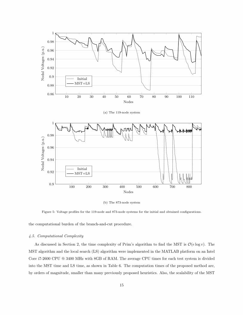
4.3. Voltage Profile

It is interesting to look into the voltage magnitudes in the initial configuration and the radial configuration

found by the MST method. For illustrative purposes, the 135-node and 873-node systems are considered

here. The voltage profiles for these test systems before and after reconfiguration are shown in Fig. 5. The

minimum and average values for the voltage magnitudes are also shown in the figure. As can be seen, a

12

Table 3: Comparison of The Best Possible Configuration and Meshed Network

Test Case P1(kW)1 P2(kW)2 ∆P (%)3 Open Lines

14-node 427.814 427.814 0 -

33-node 123.291 123.253 0.03 9

70-node 198.425 198.355 0.03 51, 75, 78

84-node 462.682 459.824 0.62 13, 63, 83, 84

119-node 819.359 818.342 0.12 23, 51, 75, 129, 130

135-node 271.846 270.83 0.37 84, 106, 135, 138

873-node 990.336 986.346 0.40132, 241, 412, 451, 596,

639, 882, 888, 890, 900

1 Losses for meshed network.2 Losses for best-known configuration. 3 Relative difference.

Table 4: Comparison of Network Losses Obtained by The Proposed Algorithms and Other References

#NodesLosses(kW)

ρ(%)i ε1ii ε2

iii ε3iv

MIQCP [20] MST LS DISTOP [4]

14 468.3 468.3 468.3 468.3 8.9 0 0 0

33 139.5 140.7 139.9 139.5 31.0 0.8 0.2 0

70 201.4 208.7 203.6 203.9 10.5 3.6 1.1 1.2

84 469.9 471.7 470.08 471.4 11.3 0.38 0.04 0.32

119 869.7 894.3 883.5 891.9 31.9 2.8 1.5 2.5

135 280.2 289.4 286.4 295.9 10.6 3.3 2.2 5.6

415 2352.4 2358.6 2355.3 2357.2 11.4 0.26 0.12 0.20

873 991.3 1001.9 1000.3 991.8 70.1 0.92 0.76 0.05

10476 N/A 8173.4 8158.1 - 47.5 N/A N/A N/A

i Loss reduction by MST+LS w.r.t the initial configuration.ii Relative optimality gap for the MST solution (%). iii Relative optimality gap for

the LS solution (%). iv Relative optimality gap for the DISTOP solution (%).

13

Table 5: Radial Configurations Obtained by The LS Algorithm

#Nodes Tie Switches

14 7,8,16

33 7,9,14,28,32

70 14,30,39,45,51,66,71,75,76,77,78

84 7,34,39,42,63,72,83,84,86,89,90,92

119 23,26,34,39,42,52,58,70,73,75,95,109,122,129,130

135 9,35,51,54,90,96,106,126,135,136,138,141,143,144,145,146,147,148,150,151,155

415

7,13,34,39,42,63,72,83,84,86,89,90,92,103,109,130,135,138,159,168,179,180,182,185,186,

188,199,225,231,234,255,264,274,276,278,280,281,282,284,295,321,327,330,351,360,370,372,

374,376,377,378,380,391,417,423,426,447,456,466,468,470,472,473,474,476,481,482,483,484,

485,486,487,488

87384,130,144,159,190,282,288,306,330,409,412,434,451,494,596,616,629,631,637,698,818,

843,885,888,890,896,900

significant improvement in voltage profiles has been achieved. These observations support the idea that the

radial network obtained by the MST routine provides improved voltage profiles.

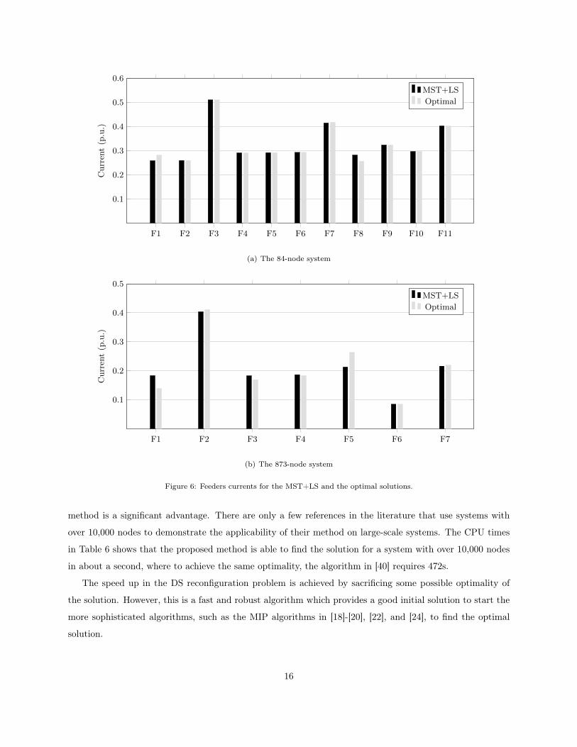
4.4. Feeders Loading

Although it is not its explicit objective, the minimum-loss network reconfiguration normally results in a

moderate load balance among all the feeders [34]. However, there are cases in which a good load balance

cannot be achieved due to the increment in the losses that would be imposed. Another case is when there is

no connection between one cluster of feeders to the other cluster. In this case, every cluster can be optimized

independently because they do not have any interdependencies. For instance, for the 84-node system in [36],

Feeders F1, F7, and F8 are in one cluster and the rest are in another cluster. No branch exchange can be

performed between these two clusters to reduce losses or improve the load balance. Therefore, maintaining

a perfect load balance may not be achievable in some cases. For illustrative purposes, the feeder currents

are shown in Fig. 6 for the 84-node and the 873-node systems, when the network is reconfigured for loss

reduction using the MST+LS method. As can be seen, the MST+LS solution generates fairly close currents

to the ones in the optimal solution.

It is of importance to notice that the main objective of the reconfiguration here is to minimize the losses,

not to find the best-possible load balance among the feeders. In order to balance the load and minimize the

losses simultaneously, a multi-objective optimization problem needs to be solved. The solution provided by

the MST+LS routine is also a good initial solution to start such multi-objective optimizations and reduce

14

10 20 30 40 50 60 70 80 90 100 1100.86

0.88

0.9

0.92

0.94

0.96

0.98

1

Nodes

NodalVoltages

(p.u.)

Initial

MST+LS

(a) The 119-node system

100 200 300 400 500 600 700 8000.9

0.92

0.94

0.96

0.98

1

Nodes

NodalVoltages

(p.u.)

Initial

MST+LS

(b) The 873-node system

Figure 5: Voltage profiles for the 119-node and 873-node systems for the initial and obtained configurations.

the computational burden of the branch-and-cut procedure.

4.5. Computational Complexity

As discussed in Section 2, the time complexity of Prim’s algorithm to find the MST is O(e log v). The

MST algorithm and the local search (LS) algorithm were implemented in the MATLAB platform on an Intel

Core i7-2600 CPU @ 3400 MHz with 8GB of RAM. The average CPU times for each test system is divided

into the MST time and LS time, as shown in Table 6. The computation times of the proposed method are,

by orders of magnitude, smaller than many previously proposed heuristics. Also, the scalability of the MST

15

F1 F2 F3 F4 F5 F6 F7 F8 F9 F10 F11

0.1

0.2

0.3

0.4

0.5

0.6

Current(p.u.)

MST+LS

Optimal

(a) The 84-node system

F1 F2 F3 F4 F5 F6 F7

0.1

0.2

0.3

0.4

0.5

Current(p.u.)

MST+LS

Optimal

(b) The 873-node system

Figure 6: Feeders currents for the MST+LS and the optimal solutions.

method is a significant advantage. There are only a few references in the literature that use systems with

over 10,000 nodes to demonstrate the applicability of their method on large-scale systems. The CPU times

in Table 6 shows that the proposed method is able to find the solution for a system with over 10,000 nodes

in about a second, where to achieve the same optimality, the algorithm in [40] requires 472s.

The speed up in the DS reconfiguration problem is achieved by sacrificing some possible optimality of

the solution. However, this is a fast and robust algorithm which provides a good initial solution to start the

more sophisticated algorithms, such as the MIP algorithms in [18]-[20], [22], and [24], to find the optimal

solution.

16

Table 6: Comparison of CPU Times for Different Methods

System MST LS Reference 1 Reference 2

33-node 0.015 0.022 7.2 ([9]) 0.3 ([29])

70-node 0.021 0.085 3 ([35]) 2.4 ([41])

84-node 0.023 0.151 36.15 ([36]) 0.3 ([29])

119-node 0.023 0.261 8.61 ([9]) 9.04 ([37])

135-node 0.026 0.551 7.3 ([18]) 0.4 ([29])

873-node 0.048 4.85 20.9 ([40]) 874 ([19])

10476-node 1.360 37.11 472 ([40]) -

5. Conclusion

The problem of distribution system reconfiguration for loss reduction is mapped into a minimum spanning

tree (MST) problem, for which efficient solution methods have been developed in the literature. A relative

optimality gap of less than 2.2% was achieved for several test systems. The main highlights of the present

framework are summarized here, as follows:

• The proposed algorithms guarantee the radiality of the final configuration.

• The MST algorithm is a low-cost heuristic that provides a solution with small optimality gap.

• The proposed local search method which is based on sensitivity factors is able to quickly polish the

MST solution.

• The MST+LS solution can be readily used as an initial solution for a direct mathematical optimization

such as MIP methods.

The application of the proposed heuristics to improve the branch-and-cut procedure is currently under

development by the authors. By applying the MST+LS algorithm instead of the default heuristics applied

in commercial solvers, it is expected to substantially reduce the processing time.

References

[1] H. Ahmadi, S. Mohseni, A. A. Shayegani Akmal, Electromagnetic fields near transmission lines-problems

and solutions, Iran. J. Environ. Health. Sci. Eng. 7 (2) (2010) 181–188.

[2] S. Civanlar, J. J. Grainger, H. Yin, S. S. H. Lee, Distribution feeder reconfiguration for loss reduction,

IEEE Trans. Power Del. 3 (3) (1988) 1217–1223.

17

[3] M. E. Baran, F. F. Wu, Network reconfiguration in distribution systems for loss reduction and load

balancing, IEEE Trans. Power Del. 4 (2) (1989) 1401–1407.

[4] D. Shirmohammadi, H. W. Hong, Reconfiguration of electric distribution networks for resistive line

losses reduction, IEEE Trans. Power Del. 4 (2) (1989) 1492–1498.

[5] M. Lavorato, J. F. Franco, M. J. Rider, R. Romero, Imposing radiality constraints in distribution system

optimization problems, IEEE Trans. Power Syst. 27 (1) (2012) 172–180.

[6] H. Ahmadi, J. R. Marti, Mathematical representation of radiality constraint in distribution system

reconfiguration problem, Int. J. Elect. Power & Energy Syst. 64 (2015) 293–299.

[7] J. Mendoza, R. Lopez, D. Morales, E. Lopez, P. Dessante, R. Moraga, Minimal loss reconfiguration

using Genetic Algorithms with restricted population and addressed operators: real application, IEEE

Trans. Power Syst. 21 (2) (2006) 948–954.

[8] H. D. de Macedo Braz, B. A. de Souza, Distribution network reconfiguration using Genetic Algorithms

with sequential encoding: subtractive and additive approaches, IEEE Trans. Power Syst. 26 (2) (2011)

582–593.

[9] R. Srinivasa Rao, S. V. L. Narasimham, M. Ramalinga Raju, A. Srinivasa Rao, Optimal network

reconfiguration of large-scale distribution system using Harmony search algorithm, IEEE Trans. Power

Syst. 26 (3) (2011) 1080–1088.

[10] Y. Jeon, J. Kim, J. Kim, J. Shin, K. Lee, An efficient Simulated Annealing Algorithm for network

reconfiguration in large-scale distribution systems, IEEE Trans. Power Del. 17 (4) (2002) 1070–1078.

[11] H. Salazar, R. Gallego, R. Romero, Artificial Neural Networks and clustering techniques applied in the

reconfiguration of distribution systems, IEEE Trans. Power Del. 21 (3) (2006) 1735–1742.

[12] C. Wang, H.-Z. Cheng, Optimization of network configuration in large distribution systems using Plant

Growth simulation algorithm, IEEE Trans. Power Syst. 23 (1) (2008) 119–126.

[13] Y. Hayashi, J. Matsuki, Loss minimum configuration of distribution system considering n-1 security of

dispersed generators, IEEE Trans. Power Syst. 19 (1) (2004) 636–642.

[14] W. Wu, M. Tsai, Application of enhanced integer coded Particle Swarm Optimization for distribution

system feeder reconfiguration, IEEE Trans. Power Syst. 26 (3) (2011) 1591–1599.

[15] Y.-K. Wu, C.-Y. Lee, L.-C. Liu, S.-H. Tsai, Study of reconfiguration for the distribution system with

distributed generators, IEEE Trans. Power Del. 25 (3) (2010) 1678–1685.

18

[16] H. M. Khodr, J. Martinez-Crespo, M. A. Matos, J. Pereira, Distribution systems reconfiguration based

on OPF using Benders decomposition, IEEE Trans. Power Del. 24 (4) (2009) 2166–2176.

[17] K. L. Butler, N. D. R. Sarma, V. Ragendra Prasad, Network reconfiguration for service restoration in

shipboard power distribution systems, IEEE Trans. Power Syst. 16 (4) (2001) 653–661.

[18] R. A. Jabr, R. Singh, B. C. Pal, Minimum loss network reconfiguration using mixed-integer convex

programming, IEEE Trans. Power Syst. 27 (2) (2012) 1106–1115.

[19] J. A. Taylor, F. S. Hover, Convex models of distribution system reconfiguration, IEEE Trans. Power

Syst. 27 (3) (2012) 1407–1413.

[20] H. Ahmadi, J. R. Martí, Distribution system optimization based on a linear power flow formulation,

IEEE Trans. Power Del. Early Access.

[21] H. P. Schmidt, N. Ida, N. Kagan, J. C. Guaraldo, Fast reconfiguration of distribution systems considering

loss minimization, IEEE Trans. Power Syst. 20 (3) (2005) 1311–1319.

[22] S. Khushalani, J. M. Solanki, N. N. Schulz, Optimized restoration of unbalanced distribution systems,

IEEE Trans. Power Syst. 22 (2) (2007) 624–630.

[23] J. Martí, H. Ahmadi, L. Bashualdo, Linear power-flow formulation based on a voltage-dependent load

model, IEEE Trans. Power Del. 28 (3) (2013) 1682–1690.

[24] J. F. Franco, M. J. Rider, M. Lavorato, R. Romero, A mixed-integer LP model for the reconfiguration of

radial electric distribution systems considering distributed generation, Elect. Power Syst. Res. 97 (2013)

51–60.

[25] IBM, IBM ILOG CPLEX Optimization Studio CPLEX User’s Manual, 12th Edition (2011).

[26] Gurobi Optimization Inc., GUROBI Optimizer Reference Manual.

[27] A. Carcamo-Gallardo, L. Garcia-Santander, J. E. Pezoa, Greedy reconfiguration algorithms for medium-

voltage distribution networks, IEEE Trans. Power Del. 24 (1) (2009) 328–337.

[28] M. Guimarães, C. Castro, R. Romero, Distribution systems operation optimisation through reconfig-

uration and capacitor allocation by a Dedicated Genetic Algorithm, IET Gen. Trans. & Dist. 4 (11)

(2010) 1213–1222.

[29] E. M. Carreno, R. Romero, A. Padilha-Feltrin, An efficient codification to solve distribution network

reconfiguration for loss reduction problem, IEEE Trans. Power Syst. 23 (4) (2008) 1542–1551.

19

[30] J. B. Kruskal, On the shortest spanning subtree of a graph and the traveling salesman problem, Pro-

ceedings of the American Mathematical society 7 (1) (1956) 48–50.

[31] R. C. Prim, Shortest connection networks and some generalizations, Bell system technical journal 36 (6)

(1957) 1389–1401.

[32] D. A. Bader, C. Guojing, Fast shared-memory algorithms for computing the minimum spanning forest

of sparse graphs, J. Para. Dist. Comp. 66 (11) (2006) 1366–1378.

[33] S. V. Pemmaraju, S. S. Skiena, Computational Discrete Mathematics: Combinatorics and Graph Theory

with Mathematica, Cambridge University Press, 2003.

[34] M. A. Kashem, M. Moghavvemi, Maximizing radial voltage stability and load balancing via loss min-

imization in distribution networks, in: Int. Conf. Energy Man. Power Del., Vol. 1, IEEE, 1998, pp.

91–96.

[35] D. Das, A fuzzy multiobjective approach for network reconfiguration of distribution systems, IEEE

Trans. Power Del. 21 (1) (2006) 202–209.

[36] C. Su, C. Lee, Network reconfiguration of distribution systems using improved mixed-integer hybrid

differential evolution, IEEE Trans. Power Del. 18 (3) (2003) 1022–1027.

[37] D. Zhang, Z. Fu, L. Zhang, An improved TS algorithm for loss-minimum reconfiguration in large-scale

distribution systems, Elect. Power Syst. Res. 77 (5-6) (2007) 685–694.

[38] J. R. S. Mantovani, F. Casari, R. A. Romero, Reconfiguraçäo de sistemas de distribuiçäo radiais uti-

lizando o critério de queda de tensäo, SBA Controle and Automaçäo 11 (3) (2000) 150–159.

[39] R. Kavasseri, C. Ababei, Reds: Repository of distribution systems (2013).

URL http://venus.ece.ndsu.nodak.edu/~kavasseri/reds.html

[40] C. Ababei, R. Kavasseri, Efficient network reconfiguration using minimum cost maximum flow-based

branch exchanges and random walks-based loss estimations, IEEE Trans. Power Syst. 26 (1) (2011)

30–37.

[41] E. R. Ramos, A. G. Exposito, J. R. Santos, F. L. Iborra, Path-based distribution network modeling:

application to reconfiguration for loss reduction, IEEE Trans. Power Syst. 20 (2) (2005) 556–564.

20