minimum information loss algorithm
TRANSCRIPT
1
MIL DISCRETIZATION ALGORITHM (FOR DESIGN OF DATA DISCRETIZOR FOR CLASSIFICATION PROBLEMS)
Project Guide –Prof Bikash.K.SarkarMembers -Shashidhar Sundareisan (BE/1343/08) and Gourab Mitra (BE/1232/08)
04/18/2023

04/18/2023 2
Introduction
Discretization is concerned with the process of transferring continuous models and equations into discrete counterparts.
This process is usually carried out as a first step toward making them suitable for numerical evaluation and implementation on digital computers.

04/18/2023 3
Four scans in MIL
Scan 1 : To calculate dmax and dmin
Scan 2: To calculate CTS(Calculated Threshold) for n intervals between dmax and dmin. Width of the interval (dmax – dmin)/n
Scan 3: To calculate optimal merged sub-intervals
Scan 4: To discretize the attribute to one of the optimal merged sub-intervals

04/18/2023 4
Example
Name CGPA Grade
Alice 6.90 Average
Bob 7.90 Good
Catherine 8.00 Excellent
Doug 5.70 Poor
Elena 7.00 Average
…… ….. ……
• CGPA is a continuous attribute• s = 4 {‘Excellent’,’Good’,’Average’,’Poor’}• c = 3 (constant value chosen by the user)• n = c . s (no. of sub-intervals) = 12• m = 88 (instances of training data)

04/18/2023 5
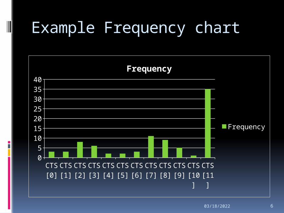
Here, dmin = 5.7 and dmax = 8.0 TS = m/n = 88/12 ≈ 7 We divide the range into 12 sub-
intervalsInterval CTS
5.7 – 5.975 1
5.975 – 6.25 2
6.25 – 6.525 6
6.525 – 6.8 20
6.8 – 7.075 15
… …
04/18/2023 6
Example Frequency chart
CTS[0
]
CTS[1
]
CTS[2
]
CTS[3
]
CTS[4
]
CTS[5
]
CTS[6
]
CTS[7
]
CTS[8
]
CTS[9
]
CTS[1
0]
CTS[1
1]0
5
10
15
20
25
30
35
40
Frequency
Frequency

04/18/2023 7
In the first interval, Tot_CTS < TS/3 . So, we merge it with the next interval.
Update Tot_CTS= Tot_CTS + CTS[1] (= 3 + 3)
Update TS = TS + m/n (= 12 + 12)

04/18/2023 8
CTS[0]
CTS[1]
CTS[2]
CTS[3]
CTS[4]
CTS[5]
CTS[6]
CTS[7]
CTS[8]
CTS[9]
CTS[10]
0
5
10
15
20
25
30
35
40
Frequency
Frequency
04/18/2023 9
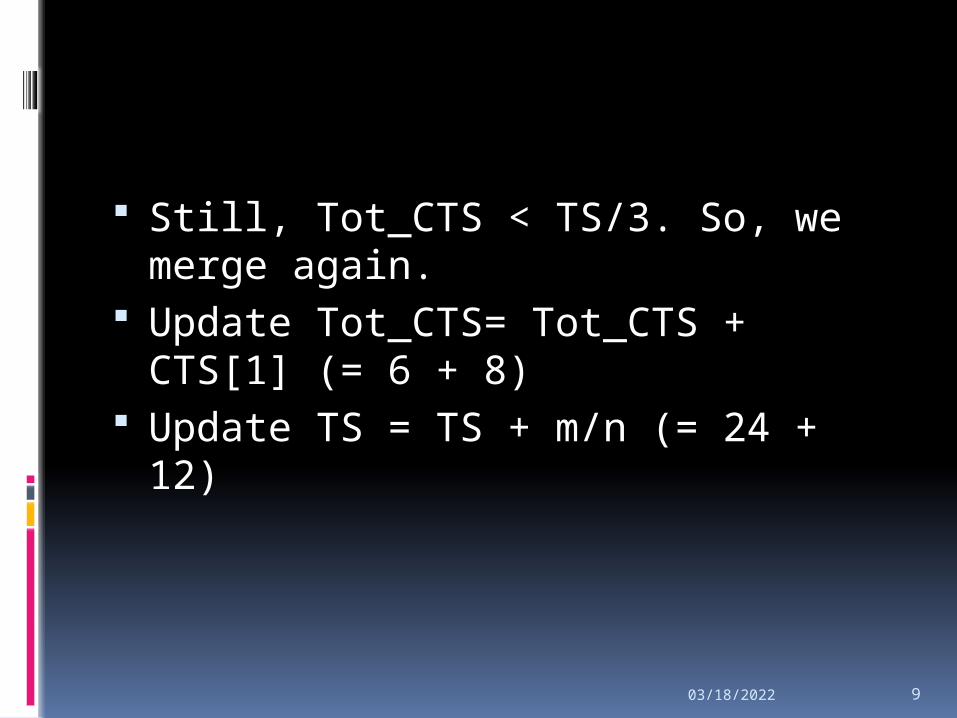
Still, Tot_CTS < TS/3. So, we merge again.
Update Tot_CTS= Tot_CTS + CTS[1] (= 6 + 8)
Update TS = TS + m/n (= 24 + 12)

04/18/2023 10
CTS[0]
CTS[1]
CTS[2]
CTS[3]
CTS[4]
CTS[5]
CTS[6]
CTS[7]
CTS[8]
CTS[9]
0
5
10
15
20
25
30
35
40
Frequency
Frequency
04/18/2023 11
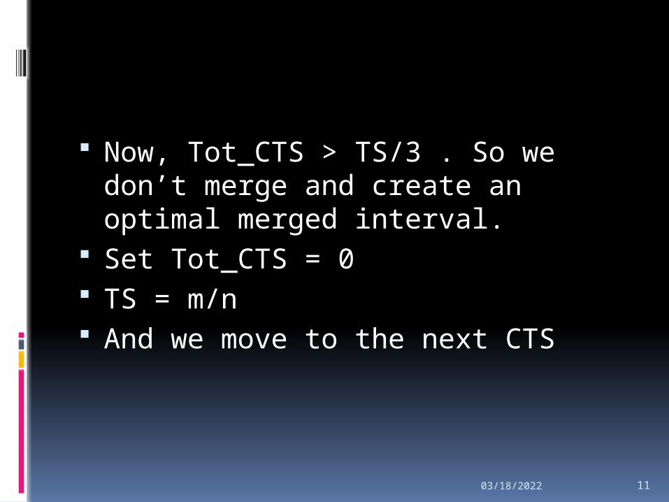
Now, Tot_CTS > TS/3 . So we don’t merge and create an optimal merged interval.
Set Tot_CTS = 0 TS = m/n And we move to the next CTS

04/18/2023 12
CTS[0]
CTS[1]
CTS[2]
CTS[3]
CTS[4]
CTS[5]
CTS[6]
CTS[7]
CTS[8]
CTS[9]
0
2
4
6
8
10
12
14
16
FrequencyOptimal Merged Sub-interval

04/18/2023 13
In this case, Tot_CTS > TS / 3. So we don’t merge and create another optimal merged sub-interval

04/18/2023 14
CTS[0]
CTS[1]
CTS[2]
CTS[3]
CTS[4]
CTS[5]
CTS[6]
CTS[7]
CTS[8]
CTS[9]
0
2
4
6
8
10
12
14
16
FrequencyOptimal Merged Sub-interval

04/18/2023 15
CTS[0]
CTS[1]
CTS[2]
CTS[3]
CTS[4]
CTS[5]
CTS[6]
0
2
4
6
8
10
12
14
16
18
20
FrequencyOptimal Merged Sub-interval

04/18/2023 16
Final Frequency Chart
CTS[0] CTS[1] CTS[2] CTS[3] CTS[4]0
5
10
15
20
25
30
35
40
45
FrequencyOptimal Merged Sub-interval
04/18/2023 17
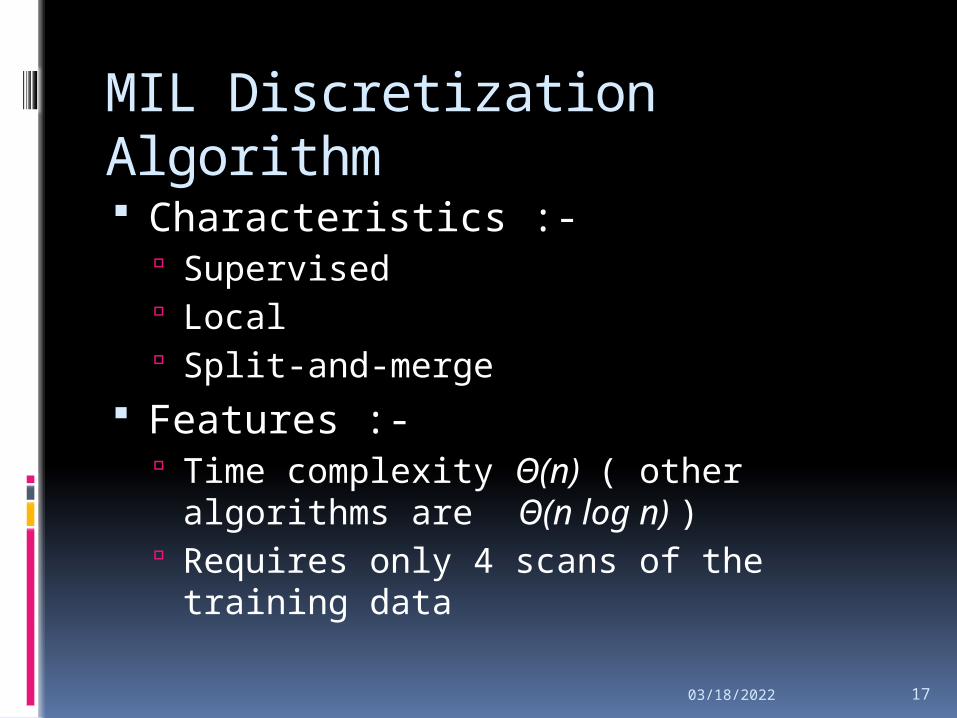
MIL Discretization Algorithm Characteristics :-
Supervised Local Split-and-merge
Features :- Time complexity Θ(n) ( other algorithms
are Θ(n log n) ) Requires only 4 scans of the training
data
04/18/2023 18
Scope for research
Optimize value of C Optimize algorithm for TS/ k (in
previous slides, we had k=3) Improving logic of the discretizer

04/18/2023 19
Uniform Distribution ?
CTS[0
]
CTS[1
]
CTS[2
]
CTS[3
]
CTS[4
]
CTS[5
]
CTS[6
]
CTS[7
]
CTS[8
]
CTS[9
]
CTS[1
0]
CTS[1
1]0
1
2
3
4
5
6
7
Frequency
Frequency
04/18/2023 20
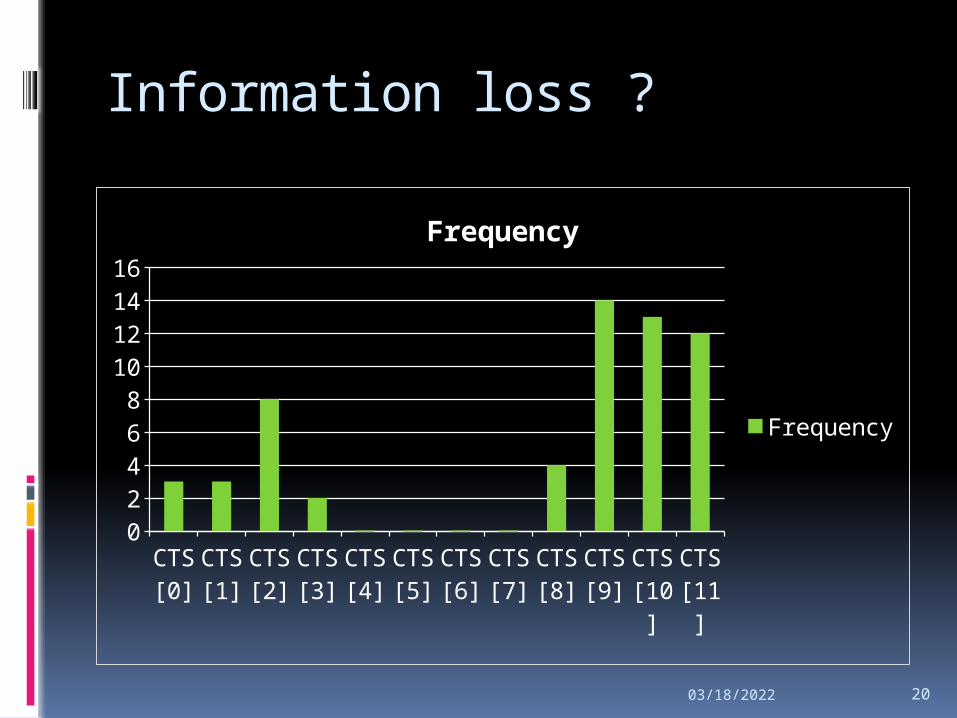
Information loss ?
CTS[0
]
CTS[1
]
CTS[2
]
CTS[3
]
CTS[4
]
CTS[5
]
CTS[6
]
CTS[7
]
CTS[8
]
CTS[9
]
CTS[1
0]
CTS[1
1]0
2
4
6
8
10
12
14
16
Frequency
Frequency

04/18/2023 21
Optimize the value of C
Datasets used : Iris, Haberman, transfusion and vertebrae column
Testing for c = 1 to 25 in each of these data sets
Using Weka to compare classfication accuracy with undiscretized data (J48 classifier)

04/18/2023 22
DEMO…
04/18/2023 23
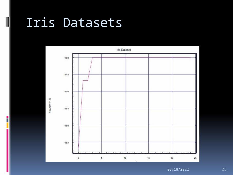
Iris Datasets

04/18/2023 24
Haberman Data

04/18/2023 25
Transfusion Data
04/18/2023 26
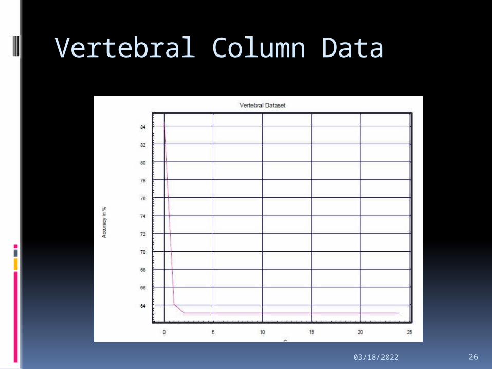
Vertebral Column Data

04/18/2023 27
Conclusion
Value of % accuracy of classification stabilizes after a certain value of C and remains constant
A steep decrease in % accuracy of classification is noted in certain cases when we deviate from continuous to discretized data by the algorithm. This warrants further probe into the algorithm.
04/18/2023 28
References
UCI Machine Learning Repository – the source for all datasets used in the project
MIL: a data discretisation approach by Bikash Kanti Sarkar, Shib Sankar Sana, Kripasindhu Chaudhuri - International Journal of Data Mining, Modelling and Management 2011 - Vol. 3, No.3 pp. 303 – 318
Oracle.com Online Javadoc

04/18/2023 29
THANK YOU