minimizing temperature droop and power line flicker in a
TRANSCRIPT

Rochester Institute of TechnologyRIT Scholar Works
Theses Thesis/Dissertation Collections
5-1-2011
Minimizing temperature droop and power lineflicker in a lamp heated xerographic fusing systemJeffrey Swing
Follow this and additional works at: http://scholarworks.rit.edu/theses
This Thesis is brought to you for free and open access by the Thesis/Dissertation Collections at RIT Scholar Works. It has been accepted for inclusionin Theses by an authorized administrator of RIT Scholar Works. For more information, please contact [email protected].
Recommended CitationSwing, Jeffrey, "Minimizing temperature droop and power line flicker in a lamp heated xerographic fusing system" (2011). Thesis.Rochester Institute of Technology. Accessed from
Minimizing Temperature Droop and
Power Line Flicker in a Lamp Heated
Xerographic Fusing System
By
Jeffrey N. Swing
A Thesis Submitted in Partial Fulfillment of the Requirements for Master
of Science in Mechanical Engineering
Approved by:
Department of Mechanical Engineering Committee
Dr. Tuhin Das, Thesis Advisor
Dr. Agamemnon Crassidis
Dr. Eric Hamby
Dr. Mark Kempski
Dr. Edward Hensel
Rochester Institute of Technology
Rochester, New York 14623
May 2011
Permission to Reproduce the Thesis
Title: Minimizing Temperature Droop and Power Line Flicker in a
Lamp Heated Xerographic Fusing System
I, Jeffrey N. Swing, hereby grant permission to the Wallace Memo-
rial Library of Rochester Institute of Technology to reproduce my thesis
in whole or part. Any reproduction will not be for commercial use or profit.
Jeffrey N. Swing
XEROX©, Nuvera, and iGen, are trademarks of XEROX CORPORA-
TION.

Abstract
Minimizing Temperature Droop and Power Line Flicker in a Lamp
Heated Xerographic Fusing System
Jeffrey N. Swing
Supervising Professor: Dr. Tuhin Das
Fuser roll temperature is one of the most important parameters affect-
ing the performance of a xerographic fusing system. Temperature must be
tightly controlled to ensure consistency of image permanence and quality,
usually with a heating lamp. To reduce lighting flicker, International Elec-
trotechnical Commission (IEC) regulations limit the effects that the heating
lamp can have on a mains power system. To meet these constraints, power
delivery to the lamp is slowed down and transient performance of the tem-
perature control system is reduced. This is especially prevalent at the start
of a print job where the thermal system transitions from a low power state
to a high one.
An existing thermal model of a fusing system is extended to cover a range
of printable media. The thermal and electrical behaviors of the heating lamp
and power system are modeled. The fast power system model is solved
ahead of time and results stored in a lookup table for use with the slower
lamp and fuser thermal models. With a complete thermal and electrical
iii

model, the variability of the temperature transients observed experimentally
is replicated.
With the system characterized and with the development of a validated
model, an open loop optimal control boundary value problem is formulated
to minimize temperature transients while meeting the electrical constraints.
After finding the solution for the nominal startup sequence, a second level
optimization is carried out with . A control trajectory is found for the nomi-
nal case that narrowly misses the performance objective at the beginning of
the job under the stress loading condition. Improving machine timing does
not yield significant improvement.
A simple feedforward controller is synthesized to use the optimal control
results in a practical controller. Knowledge of the system is still needed to
find the power level the system must transition to.
iv

Acknowledgments
I would like to thank Dr. Tuhin Das for his guidance and support as
my advisor throughout this project. I have learned a lot of material outside
the scope of coursework at RIT, and am looking forward to applying this
knowledge in my career.
I would like to thank Eric Hamby for supporting this project on the com-
mittee and providing guidance in presenting research. As I’ve been involved
in product development for 10 years, he has given me a new perspective
from the research side of Xerox.
Greg Weselak took the time to help me understanding the intricacies of
the power controller in this work, his help was invaluable to this work and I
cannot thank him enough.
Many thanks to Yongsoon Eug, Eric Hamby, and Chuck Facchini for the
collaboration in the initial development of the thermal model that spawned
this work.
v

I could not have done this project and completed my coursework without
the continued support of my managers at Xerox. Thank you Doug Wilkins,
Christine Keenan, Erwin Ruiz, and Brian Perry for giving me the freedom
and the time to pursue my studies and this work within the busy product
development cycle.
This work and my graduate studies would not have been possible without
the loving support of my wife Amelia, I love you.
vi
Contents
Abstract . . . . . . . . . . . . . . . . . . . . . . . . . . . . . . . iii
Acknowledgments . . . . . . . . . . . . . . . . . . . . . . . . . v
1 Introduction . . . . . . . . . . . . . . . . . . . . . . . . . . . 1
1.1 Motivation . . . . . . . . . . . . . . . . . . . . . . . . . . . 1
1.2 Outline . . . . . . . . . . . . . . . . . . . . . . . . . . . . 3
2 Historical and Literature Review . . . . . . . . . . . . . . . 5
2.1 Roll Fusing Primer . . . . . . . . . . . . . . . . . . . . . . 6
2.2 Temperature Control in Fusing . . . . . . . . . . . . . . . . 9
2.3 Heat Equation and Lumped Mass Simplification . . . . . . . 12
2.4 Lumped Parameter Hybrid Modeling . . . . . . . . . . . . . 17
2.5 Lamp Filament Modeling . . . . . . . . . . . . . . . . . . . 18
2.6 Power Line Flicker . . . . . . . . . . . . . . . . . . . . . . 19
2.7 Fuser Power Controller . . . . . . . . . . . . . . . . . . . . 23
2.8 Multiple Time Scales . . . . . . . . . . . . . . . . . . . . . 23
2.9 Variational Calculus Approach to Optimal Control . . . . . . 25
2.10 State Feedback Control . . . . . . . . . . . . . . . . . . . . 27
3 Fuser thermal model development . . . . . . . . . . . . . . . 29
3.1 Energy Balance Equations . . . . . . . . . . . . . . . . . . 30
3.2 Assumptions . . . . . . . . . . . . . . . . . . . . . . . . . 34
3.3 Experimental Setup . . . . . . . . . . . . . . . . . . . . . . 37
vii

3.4 Parameter Estimation - Step 1 . . . . . . . . . . . . . . . . 40
3.5 Parameter Estimation - Step 2 . . . . . . . . . . . . . . . . 41
3.6 Discussion . . . . . . . . . . . . . . . . . . . . . . . . . . . 45
4 Problem Statement . . . . . . . . . . . . . . . . . . . . . . . 46
5 Fuser thermal model refinement . . . . . . . . . . . . . . . . 48
5.1 Thermal load sliding factor . . . . . . . . . . . . . . . . . . 48
5.2 Discussion . . . . . . . . . . . . . . . . . . . . . . . . . . . 53
6 Lamp filament model development . . . . . . . . . . . . . . 55
6.1 Tungsten Filament Resistance . . . . . . . . . . . . . . . . 56
6.2 Energy balance equations . . . . . . . . . . . . . . . . . . . 57
6.3 Experimental Setup . . . . . . . . . . . . . . . . . . . . . . 60
6.4 Parameter Estimation . . . . . . . . . . . . . . . . . . . . . 62
6.5 Bandwidth and system response . . . . . . . . . . . . . . . 65
6.6 Average Power Input . . . . . . . . . . . . . . . . . . . . . 67
6.7 Lamp voltage to power relationship . . . . . . . . . . . . . 70
6.8 Lamp simulation and flicker response . . . . . . . . . . . . 72
6.9 Discussion . . . . . . . . . . . . . . . . . . . . . . . . . . . 75
7 Power electronics model development . . . . . . . . . . . . . 76
7.1 Fuser Power Controller Electric Model . . . . . . . . . . . . 77
7.2 Lamp and Power Electronics Model . . . . . . . . . . . . . 78
7.3 Average power and lookup table . . . . . . . . . . . . . . . 79
7.4 Flicker Response . . . . . . . . . . . . . . . . . . . . . . . 84
7.5 Discussion . . . . . . . . . . . . . . . . . . . . . . . . . . . 86
8 Combined thermal and electrical model . . . . . . . . . . . . 87
8.1 Model Block Diagram . . . . . . . . . . . . . . . . . . . . 88
viii

8.2 Current Controls and Behavior . . . . . . . . . . . . . . . . 89
8.3 System model performance . . . . . . . . . . . . . . . . . . 92
8.4 Alternate PID tuning . . . . . . . . . . . . . . . . . . . . . 97
8.5 Discussion . . . . . . . . . . . . . . . . . . . . . . . . . . . 99
9 Open-loop optimal control problem . . . . . . . . . . . . . . 101
9.1 Integrated Control . . . . . . . . . . . . . . . . . . . . . . . 102
9.2 Cost Functional . . . . . . . . . . . . . . . . . . . . . . . . 103
9.3 Optimal control boundary value problem . . . . . . . . . . . 105
9.4 Flight plan . . . . . . . . . . . . . . . . . . . . . . . . . . . 108
9.5 Optimal Trajectories . . . . . . . . . . . . . . . . . . . . . 109
9.6 Verification of power controller constraints . . . . . . . . . . 112
9.7 Second order optimization . . . . . . . . . . . . . . . . . . 115
9.8 Discussion . . . . . . . . . . . . . . . . . . . . . . . . . . . 118
10 Controller Design . . . . . . . . . . . . . . . . . . . . . . . . 121
10.1 Trajectory Parameterization . . . . . . . . . . . . . . . . . . 122
10.2 Proposed control architecture . . . . . . . . . . . . . . . . . 126
10.3 State feedback control . . . . . . . . . . . . . . . . . . . . . 129
10.4 Controller tuning and Performance . . . . . . . . . . . . . . 130
10.5 Discussion . . . . . . . . . . . . . . . . . . . . . . . . . . . 134
11 Conclusions and Future Work . . . . . . . . . . . . . . . . . 136
11.1 Conclusions . . . . . . . . . . . . . . . . . . . . . . . . . . 136
11.1.1 Complete Thermo-electric Model . . . . . . . . . . 136
11.1.2 Optimal Control . . . . . . . . . . . . . . . . . . . 136
11.1.3 Control Design . . . . . . . . . . . . . . . . . . . . 137
11.2 Suggestions for future work . . . . . . . . . . . . . . . . . . 137
11.2.1 Thermal Modeling . . . . . . . . . . . . . . . . . . 137
ix

11.2.2 Power System Modeling . . . . . . . . . . . . . . . 138
11.2.3 Control . . . . . . . . . . . . . . . . . . . . . . . . 139
Bibliography . . . . . . . . . . . . . . . . . . . . . . . . . . . . 141
A Matlab code for open-loop optimal control solution . . . . . 145
B Xerox Proprietary Information . . . . . . . . . . . . . . . . 149
B.1 Proprietary Literature Review . . . . . . . . . . . . . . . . . 149
B.1.1 Lumped Parameter Hybrid Modeling . . . . . . . . 150
B.1.2 Fuser Power Controller . . . . . . . . . . . . . . . . 151
B.2 Fuser Model Development . . . . . . . . . . . . . . . . . . 155
B.3 Problem Statement . . . . . . . . . . . . . . . . . . . . . . 156
B.4 Fuser Model Refinement . . . . . . . . . . . . . . . . . . . 158
B.5 Fuser Power Controller Electric Model . . . . . . . . . . . . 160
B.6 Lamp and Power Electronics Model . . . . . . . . . . . . . 165
B.7 Average power and lookup table . . . . . . . . . . . . . . . 167
B.8 Current Controls and Behavior . . . . . . . . . . . . . . . . 168
B.9 System model performance . . . . . . . . . . . . . . . . . . 173
B.10 Integrated Control . . . . . . . . . . . . . . . . . . . . . . . 175
B.11 Flight Plan . . . . . . . . . . . . . . . . . . . . . . . . . . . 177
B.12 Optimal Trajectories . . . . . . . . . . . . . . . . . . . . . 177
B.13 Trajectory Parameterization . . . . . . . . . . . . . . . . . . 180
B.14 Controller tuning and Performance . . . . . . . . . . . . . . 180
B.15 Matlab Code . . . . . . . . . . . . . . . . . . . . . . . . . . 180
x

List of Tables
3.1 Four-state and five-state model fit to the validation data . . . 44
5.1 Scaling factor calculated from average steady state power
by media . . . . . . . . . . . . . . . . . . . . . . . . . . . . 54
6.1 Optimum parameters for the one-state lamp model and the
Nuvera data . . . . . . . . . . . . . . . . . . . . . . . . . . 63
6.2 Optimum parameters for two-state lamp model and the Nu-
vera data . . . . . . . . . . . . . . . . . . . . . . . . . . . . 63
6.3 Model fit for two-state model and validation data . . . . . . 64
6.4 Short-term flicker (Pst values for on/off switching of the
lamp model . . . . . . . . . . . . . . . . . . . . . . . . . . 74
9.1 Flight plan and constraints for optimal control problem with
fixed switching instants. x2(0) and x1(0) in normalized units 109
10.1 Steady state values of the state vector, x1 and x2 normalized
to r2 and x3 and x4 in degrees Celsius . . . . . . . . . . . . 122
10.2 Tuned feedforward parameters . . . . . . . . . . . . . . . . 131
B.1 Model parameters for M1 and M2 . . . . . . . . . . . . . . 156
B.2 Model parameters for M3 . . . . . . . . . . . . . . . . . . . 156
B.3 Scaling factor calculated from average steady state power
by media . . . . . . . . . . . . . . . . . . . . . . . . . . . . 159
B.4 Bandwidth for each dynamic mode . . . . . . . . . . . . . . 160
xi
B.5 Switch states for the fuser power controller . . . . . . . . . 161
B.6 Parameter values for the fuser power controller simulation
in figure B.10 . . . . . . . . . . . . . . . . . . . . . . . . . 165
B.7 Flight plan and constraints for optimal control problem with
fixed switching instants . . . . . . . . . . . . . . . . . . . . 177
B.8 Steady state values of the state vector with x2 = 200, all in
degrees Celsius . . . . . . . . . . . . . . . . . . . . . . . . 177
xii
List of Figures
1.1 Temperature droop at the start of a job . . . . . . . . . . . . 2
1.2 Temperature droop example aggravated by power limiting . 3
2.1 A fuser roll pair with image side down. . . . . . . . . . . . . 7
2.2 Circumferential fuser roll temperature gradient during fusing 11
2.3 Fuser roll axial temperature gradient for a center registered
system. . . . . . . . . . . . . . . . . . . . . . . . . . . . . 12
2.4 The three different dynamic modes of a roll fusing system . 13
2.5 Temperature droop with higher standby temperature . . . . . 13
2.6 Flicker circuit . . . . . . . . . . . . . . . . . . . . . . . . . 20
2.7 Power distribution with equivalent resistance and inductance
for evaluation of flicker with a heating lamp . . . . . . . . . 21
2.8 The human eye weighting filter for flicker perceptibility . . . 22
3.1 The thermal masses and their connectivity for M1 . . . . . . 31
3.2 The thermal masses and their connectivity for M2 . . . . . . 32
3.3 The thermal masses and their connectivity for M3 . . . . . . 33
3.4 Experimental setup with temperature sensors on fuser roll . . 38
3.5 Experimental setup with temperature sensors on the pres-
sure roll . . . . . . . . . . . . . . . . . . . . . . . . . . . . 39
3.6 Model performance with the M1/M2 data set for estimation . 41
3.7 Model performance with the M1/M2 data set for validation . 42
3.8 Model performance with the M1/M2/M3 data set for esti-
mation . . . . . . . . . . . . . . . . . . . . . . . . . . . . . 43
xiii
3.9 Model performance with the M1/M2/M3 data set for vali-
dation . . . . . . . . . . . . . . . . . . . . . . . . . . . . . 44
6.1 Block diagram for one-state lamp model . . . . . . . . . . . 57
6.2 Block diagram for two-state lamp model . . . . . . . . . . . 59
6.3 Lamp cold startup data for model parameter estimation . . . 61
6.4 The model fit with a validation data set for the one-state
lamp filament model. . . . . . . . . . . . . . . . . . . . . . 64
6.5 The bandwidth of the nonlinear lamp model versus operat-
ing temperature . . . . . . . . . . . . . . . . . . . . . . . . 67
6.6 Lamp startup comparison with AC voltage and constant RMS
voltage value applied . . . . . . . . . . . . . . . . . . . . . 69
6.7 Comparision of lamp filament model prediction of resis-
tance and re-rating equation . . . . . . . . . . . . . . . . . . 71
6.8 Heating lamp circuit with equivalent line resistance and in-
ductance . . . . . . . . . . . . . . . . . . . . . . . . . . . . 72
6.9 Simulation of the power line voltage during an unconstrained
start of the Nuvera lamp . . . . . . . . . . . . . . . . . . . 73
6.10 Line voltage and flicker response for on/off control of the
lamp model . . . . . . . . . . . . . . . . . . . . . . . . . . 74
7.1 The FPC softens the on and off transitions of the heating lamp 77
7.2 Measured lamp startup with the fuser power controller . . . 78
7.3 Block diagram showing interconnectivity between lamp and
power controller subsystems . . . . . . . . . . . . . . . . . 79
7.4 A simulated cold start for 60 hertz and 50 hertz power systems 80
7.5 Comparison of flicker duty cycle with a cold lamp start . . . 82
7.6 Normalized peak lamp current as a function of filament re-
sistance and FPC duty cycle. . . . . . . . . . . . . . . . . . 83
xiv
7.7 Applied power (W) as a function of filament resistance and
FPC duty cycle. . . . . . . . . . . . . . . . . . . . . . . . . 83
7.8 Applied power (W) with current limiting as a function of
filament resistance and FPC duty cycle. . . . . . . . . . . . 84
7.9 A simulated cold start at 230 volts and 50 hertz . . . . . . . 85
8.1 The block diagram for complete thermo-electric system. . . 88
8.2 Machine data transition from standby to run with fuser power
controller, with a moderate thermal load (CX 24# paper). . . 90
8.3 Machine data transition from standby to run with the fuser
power controller, with moderate thermal load (24 lb CX pa-
per) and low line voltage. . . . . . . . . . . . . . . . . . . . 91
8.4 Model startup droop performance with the lamp off at paper
arrival case, k=1.494, 230V 50Hz line voltage. Temperature
normalized to target temperature and control performance
objective. . . . . . . . . . . . . . . . . . . . . . . . . . . . 93
8.5 Model input power and heat flow for the lamp off at paper
arrival case, k=1.494, 230V 50Hz line voltage. Cycle-up
transient portion of the simulation shown. . . . . . . . . . . 94
8.6 Model filament resistance for the lamp off at paper arrival
case, k=1.494, 230V 50 Hz line voltage . . . . . . . . . . . 95
8.7 Time to restart lamp to 100% in the power model based as
a function of shutoff time . . . . . . . . . . . . . . . . . . . 96
8.8 Model droop performance with the lamp on at paper arrival
case, k=1.494, 230V 50 Hz line voltage . . . . . . . . . . . 97
8.9 Combined model droop performance with alternate PID gain
factors. . . . . . . . . . . . . . . . . . . . . . . . . . . . . 98
8.10 Lamp input for combined model with alternate PID gain
factors. . . . . . . . . . . . . . . . . . . . . . . . . . . . . 99
xv
9.1 The multiple timing rates of the temperature control and
power control systems. . . . . . . . . . . . . . . . . . . . . 103
9.2 Optimal input trajectory for fixed switching time . . . . . . 110
9.3 Optimal state trajectory for fuser roll states x1 and x2 for
fixed switching time . . . . . . . . . . . . . . . . . . . . . . 111
9.4 Optimal state trajectory for pressure roll states x3 and x4 for
fixed switching time problem . . . . . . . . . . . . . . . . . 111
9.5 Optimal input trajectory from figure 9.2, with power system
time response. . . . . . . . . . . . . . . . . . . . . . . . . . 113
9.6 Optimal input trajectory from figure 9.2, with power re-
sponse surface. . . . . . . . . . . . . . . . . . . . . . . . . 114
9.7 Cost functional vs loading time and initial pressure roll tem-
perature for k=1 . . . . . . . . . . . . . . . . . . . . . . . . 115
9.8 Cost functional vs loading time and initial pressure roll tem-
perature for k=1.823 . . . . . . . . . . . . . . . . . . . . . 116
9.9 State trajectories for second order optimization, normalized.
State trajectories in absolute units shown in figure B.23 . . . 117
9.10 Input trajectories for second order optimization . . . . . . . 117
9.11 Comparison of disturbance rejection performance of closed
loop and optimal open-loop controllers . . . . . . . . . . . . 118
9.12 The progression of optimal trajectories for the k=1.823 case 119
10.1 The optimal state and input trajectory for k = 1 . . . . . . . 123
10.2 The optimal trajectory for k=1 with initial and final refer-
ence values . . . . . . . . . . . . . . . . . . . . . . . . . . 125
10.3 The prefiltered reference signal with step change 10.5 sec-
onds before M3 at t = 63 and critically damped second
order system with natural frequency ωn = 1/3 rad/sec . . . . 125
xvi

10.4 The proposed block diagram for the feedforward control
scheme. . . . . . . . . . . . . . . . . . . . . . . . . . . . . 126
10.5 Feedforward controller performance for k = 1 and x3(0) =
x4(0) = 25 . . . . . . . . . . . . . . . . . . . . . . . . . . 131
10.6 Input signal for feedforward controller . . . . . . . . . . . . 132
10.7 Controller comparison to optimal solution . . . . . . . . . . 133
10.8 Feedforward controller performance for k = 1.823 . . . . . . 133
10.9 Feedforward controller performance for k=1.823 and high
and low pressure roll temperatures . . . . . . . . . . . . . . 134
10.10Feedforward controller performance for midpoint k=1.4115 . 135
B.1 Fuser thermal mass connectivity . . . . . . . . . . . . . . . 151
B.2 Lamp power modulation using a zero crossing solid state relay152
B.3 Lamp power modulation with the fuser power controller . . 153
B.4 The FPC softens the on and off transitions of the heating lamp154
B.5 Measured lamp startup with the fuser power controller . . . 155
B.6 Bode magnitude plot comparing the systemmodes with nom-
inal and high thermal load for the M3 system. . . . . . . . . 159
B.7 IGBT diagram . . . . . . . . . . . . . . . . . . . . . . . . . 160
B.8 Simplified drive circuit of the fuser power controller . . . . . 161
B.9 A further simplification of the FPC schematic . . . . . . . . 162
B.10 Simulated lamp current delivered by the electronics in the
fuser power controller . . . . . . . . . . . . . . . . . . . . . 164
B.11 A closeup of the simulated lamp current with the fuser power
controller . . . . . . . . . . . . . . . . . . . . . . . . . . . 164
B.12 A simulated cold start with the combined power electronics
and lamp filament models for 208 volts, 60 Hz. . . . . . . . 166
B.13 Comparison of flicker duty cycle with a cold lamp start . . . 168
xvii

B.14 Peak lamp current (A) as a function of filament resistance
and FPC duty cycle. . . . . . . . . . . . . . . . . . . . . . . 169
B.15 Applied power (W) as a function of filament resistance and
FPC duty cycle. . . . . . . . . . . . . . . . . . . . . . . . . 169
B.16 Applied power (W) with current limiting as a function of
filament resistance and FPC duty cycle. . . . . . . . . . . . 170
B.17 Machine data transition from standby to run with fuser power
controller, with a moderate thermal load (CX 24# paper). . . 171
B.18 Machine data transition from standby to run with the fuser
power controller, with moderate thermal load (24 lb CX pa-
per) and low line voltage. . . . . . . . . . . . . . . . . . . . 172
B.19 Model startup droop performance with the lamp off at paper
arrival case, k=1.494, 230V 50Hz line voltage. . . . . . . . . 173
B.20 Model droop performance with the lamp on at paper arrival
case, k=1.494, 230V 50 Hz line voltage . . . . . . . . . . . 174
B.21 The multiple timing rates of the temperature control and
power control systems. . . . . . . . . . . . . . . . . . . . . 176
B.22 Optimal state trajectory for fuser roll states x1 and x2 for
fixed switching time . . . . . . . . . . . . . . . . . . . . . . 178
B.23 State trajectories for second order optimization . . . . . . . 178
B.24 The optimal state and input trajectory for k = 1 . . . . . . . 179
B.25 The optimal trajectory for k=1 with initial and final refer-
ence values . . . . . . . . . . . . . . . . . . . . . . . . . . 179
B.26 The prefiltered reference signal with step change 10.5 sec-
onds before M3 at t = 63 and critically damped second
order system with natural frequency ωn = 1/3 rad/sec . . . . 180
B.27 Feedforward controller performance for k = 1 and x3(0) =
x4(0) = 25 . . . . . . . . . . . . . . . . . . . . . . . . . . 181
xviii
Chapter 1
Introduction
The objective of this work is to study and minimize the temperature tran-
sients during the cycle up of a fusing system in a Xerox copier/printer. The
motivation and general description of the problem detailed in section 1.1,
followed by an outline of this work in section 1.2.
1.1 Motivation
The xerographic process arranges powdered toner particles into an image
and then attaches it temporarily to a substrate using electrostatic forces. A
fuser permanently fixes the image to the substrate using temperature and
pressure. In the production market space, the machine owner demands high
image quality and consistency. This is paramount when the output from a
printer is sold to customers. The temperature of the fusing roll is one of the
critical parameters that affect the permanence and quality of the image.
1

Surface Temp
Core Temp
Stand-byStart
10-50
Prints
Stand-by
End
Power =100% Power 10% of run with
good insulation
Run
Droop
Tem
per
ature
Figure 1.1: Temperature droop example. Source: Bott [12]
A fusing system experiences a temperature transient each time it tran-
sitions from an idle or stand by state, to a production state where imaged
prints are fused. This requires a sudden increase in the heating power to the
fusing system of an order of magnitude. A common method to combat this
temperature droop is to set the temperature set point higher as in figure 1.1.
A fuser is typically heated using a tungsten filament lamp. Changes in
power can be applied very quickly, but one drawback is the very high inrush
current when a cold lamp is first turned on. Switching a lamp on and off
causes fluctuations on the line voltage, and may cause flicker on the lighting
systems. The International Electrotechnical Commission (IEC) has placed
limitations on the allowable fluctuations on the power line flicker.
2

To combat this, the lamp power is modulated through a high speed power
controller. This has the effect of slowing down the ability to apply quick
changes to the heating lamp power. This in turn aggravates the startup
droop, as described in figure 1.2.
Surface Temp
Core Temp
Droop
Increased droop with flicker power limiting
Figure 1.2: Temperature droop example aggravated by power limiting. Adapted from
Bott [12]
Balancing the conflicting constraints of minimizing temperature transients
and minimizing power line flicker is the central problem in this work. An
existing fuser thermal model is augmented with the dynamics of the lamp
and power system. Understanding of the contributors to the system perfor-
mance has identified many areas for improvement in the control.
1.2 Outline
A review of literature and historical information relevant to the thermal
and electrical systems in this work is detailed in chapter 2. The pre-existing
3

thermal model developed for the system being studied is detailed in chap-
ter 3.
After a problem statement and performance objectives defined in chapter
4, an extension to the thermal model is presented in chapter 5.
The experiment and the parameter optimization for a thermal model of
the lamp filament is explained in chapter 6. The high speed power control
system model is derived in chapter 7. A validation of the complete model is
detailed in chapter 8, along with some observations.
The optimal control boundary value problem for nominal machine timing
is derived and solved in chapter 9. A second level analysis examines system
timing changes and dependencies on initial state. A simple feedforward
control scheme using knowledge from the optimal trajectories is detailed
in chapter 10. Conclusions and opportunities for continued research are
presented in chapter 11
4
Chapter 2
Historical and Literature Review
A basic review of the fusing process is presented in section 2.1, along
with the roll fusing embodiment. The temperature gradients complicating
the temperature control of a fuser are reviewed in section 2.2.
In this work and many of the references, thermal systems with complex
geometry are discretized into thermal masses to capture essential dynam-
ics. In section 2.3, the heat equation and the lumped mass simplification
is reviewed. Several examples of control-oriented models for modeling the
temperature control systems in Xerox fusers are presented in section 2.4.
Two models modeling the thermal response of a tungsten lamp filament
are detailed in section 2.5. The basics behind power line flicker are reviewed
in section 2.6. A review of the power controller responsible for enforcing
these constraints in the Nuvera machine is detailed in section 2.7. The the-
ory behind combining models of disparate time scales is reviewed in section
5

2.8.
The method for determining the optimal open-loop control is reviewed
in section 2.9. Several control structures used in this work are reviewed in
section 2.10.
2.1 Roll Fusing Primer
Roll fusing is the most common technology used to fuse images. A fuser
can be oriented in almost any direction; in this system the image side is face
down. A diagram of this roll pair configuration is shown in figure 2.1. The
lower roll contacting the image is called the fuser roll. The fuser roll surface
temperature is measured with a soft-touch thermistor and heated internally
with a heating lamp. A non-stick coating is applied to the outside to aid in
release of the toner. The roll on the non-image side is a deformable pressure
roller.
As detailed by Bott [12], the desired function of a fuser is to take an image
developed with powdered toner and make it permanent. A customer wants
three main things out of a fuser:
1. Durable images on their choice of substrate
2. Attractive images on their choice of substrate
3. Consistent images
6

Pressure
Roll
Fuser Roll
Toner particles
held by
electrostatic forces
Fused image
Conformable rubber layer
Non-stick
coating
Substrate (paper)
Soft-touch
temperature
sensor
Metal core
Metal core
Heating
Lamp
Fusing Nip
Figure 2.1: A fuser roll pair with image side down.
7

The image durability is measured by cohesion (toner-to-toner) and adhe-
sion (toner-to-substrate). Toner with poor cohesion will rub off on adjacent
sheets in a stack or book, or when handled. Toner with poor adhesion will
not be resistant to creasing the substrate. For example, a flyer can be folded
in thirds for mailing. Creasing on a poorly fused image area will cause the
toner to break away from the substrate.
For an image to be attractive, a particular gloss level is desired. With
poor fusing, the surface of the image will still be granular like the powdered
toner. With a well fused image, the toner has melted sufficiently and flowed
to form a high mirrored surface. Customer preference will range from a
matte finish to high gloss. Gloss is a function of the toner material properties
and the fusing process parameters. Gloss is usually measured by a specular
gloss meter with a specified incidence angle.
In color fusing, the ability to reproduce a large range of colors (called
color gamut) is desired. The four process colors (cyan, magenta, yellow,
black) are fused at the same time. The fusing process can grow or shrink the
gamut volume as adjacent toner dots may spread and mix differently based
on how well they are fused. The color gamut volume is reported in terms of
color coordinates in (L*, a*, b*) color space.
For consistent images, the fusing process parameters must be maintained
within desired ranges. The three critical process parameters in fusing are
8

temperature, pressure, and dwell (time).
1. The temperature melts the toner and determines how viscous the molten
toner becomes. The viscosity affects the flow rate of the toner, which
ultimately affects the cohesion and adhesion.
2. The pressure drives toner deformation and flow as well as conformance
of the toner to the substrate. In rough uncoated media, the pressure will
help the toner flow into the surface voids to develop good adhesion.
3. Dwell is the time a point on the paper takes to go from one side of
the fusing nip to the other. Dwell allows heat transfer to the toner and
paper, and gives time for the toner to flow under pressure.
In addition, the fusing process must be robust to variation of toner and
substrate properties, and environmental conditions specified for the ma-
chine. Specifically related to heat transfer, the media can have a range of
heat transfer properties based on the basis weight and the surface roughness
and coating.
2.2 Temperature Control in Fusing
A tungsten filament heating lamp is one way to heat the fusing system.
Suspended inside a fusing roller, radiant heat transfer takes place along the
entire inner diameter of the roller. A high emissivity coating is applied to
9
the inner diameter of the core to increase heat transfer.
When controlling temperature of the fusing process, the temperature gra-
dients are based in cylindrical coordinates. A gradient forms around the
circumference, one along the roll axis, and one radially through the layers.
The magnitude of these gradients will drive the number and placement of
temperature sensors, and the axial heat flux profile of the heating lamps.
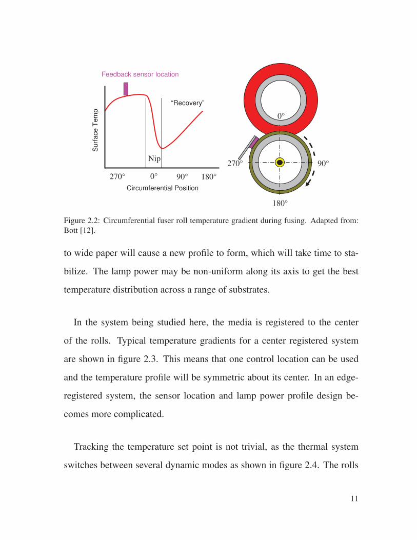
When fusing prints, a temperature gradient forms around the circumfer-
ence of the fuser roll. This is shown in figure 2.2. The heat transfer takes
place across the nip, about 345 to 15 in the diagram. A rapid temperature
drop occurs as heat is transferred to the paper, temperature recovers as the
roll rotates. Ideally, the average temperature within the nip is the temper-
ature that a control engineer would like to be able to control. Usually, the
temperature is measured upstream as close as possible to the nip, about 330
in the diagram. In this location, the temperature is fairly consistent as the
rate of change is the lowest. At location 45, the temperature is changing
rapidly and control at this location would cause large transients in the fusing
performance.
The goal of a temperature control system in a fuser is to maintain the de-
sired fusing temperature in the area contacting paper. This is compounded
by fusing substrates of different sizes back-to-back. A temperature distribu-
tion will stabilize on the fuser roll while running narrow paper. Switching
10
Circumferential Position
Surf
ace T
em
p
Nip
0° 90° 180°270°
“Recovery”
0°
180°
90°270°
Feedback sensor location
Figure 2.2: Circumferential fuser roll temperature gradient during fusing. Adapted from:
Bott [12].
to wide paper will cause a new profile to form, which will take time to sta-
bilize. The lamp power may be non-uniform along its axis to get the best
temperature distribution across a range of substrates.
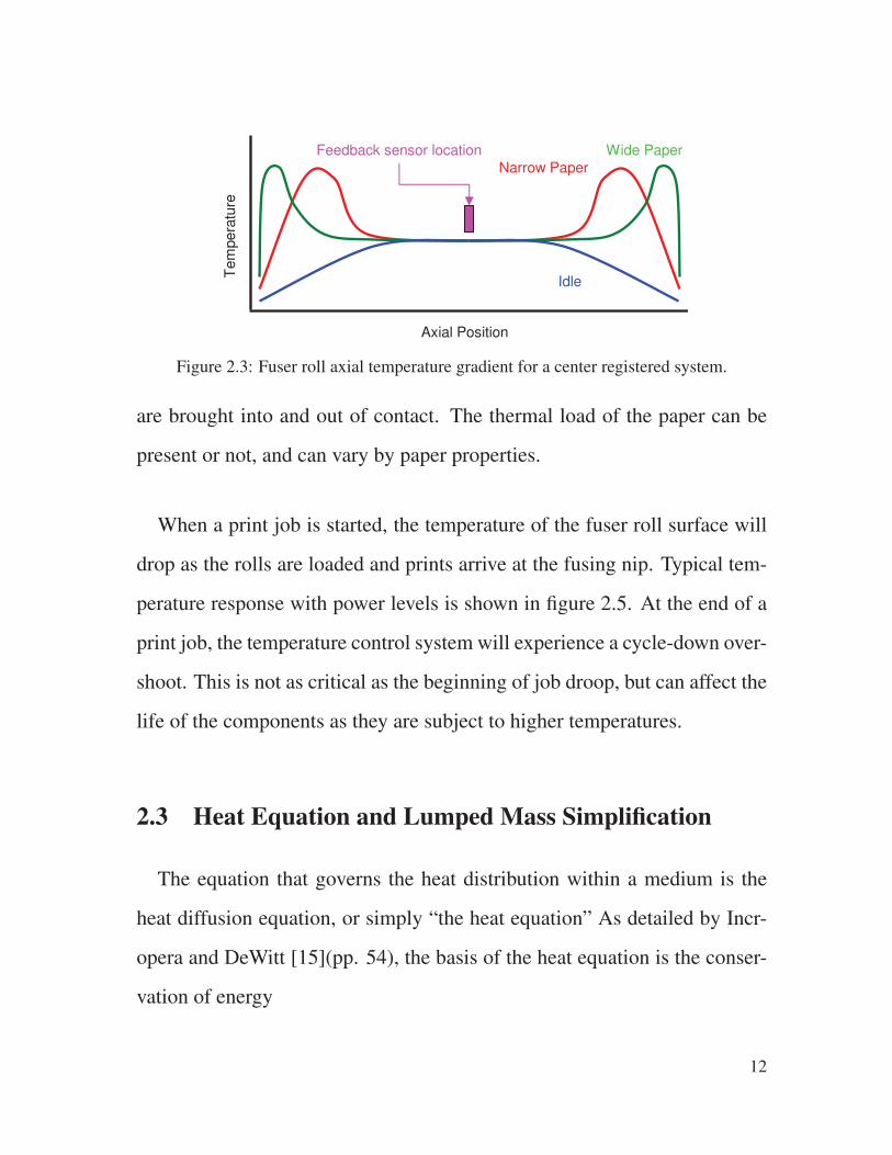
In the system being studied here, the media is registered to the center
of the rolls. Typical temperature gradients for a center registered system
are shown in figure 2.3. This means that one control location can be used
and the temperature profile will be symmetric about its center. In an edge-
registered system, the sensor location and lamp power profile design be-
comes more complicated.
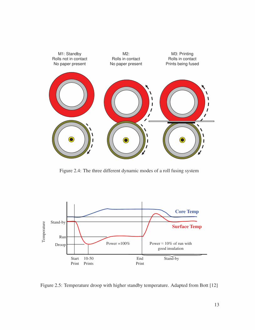
Tracking the temperature set point is not trivial, as the thermal system
switches between several dynamic modes as shown in figure 2.4. The rolls
11
Narrow Paper
Wide Paper
Idle
Feedback sensor location
Axial Position
Tem
pera
ture
Figure 2.3: Fuser roll axial temperature gradient for a center registered system.
are brought into and out of contact. The thermal load of the paper can be
present or not, and can vary by paper properties.
When a print job is started, the temperature of the fuser roll surface will
drop as the rolls are loaded and prints arrive at the fusing nip. Typical tem-
perature response with power levels is shown in figure 2.5. At the end of a
print job, the temperature control system will experience a cycle-down over-
shoot. This is not as critical as the beginning of job droop, but can affect the
life of the components as they are subject to higher temperatures.
2.3 Heat Equation and Lumped Mass Simplification
The equation that governs the heat distribution within a medium is the
heat diffusion equation, or simply “the heat equation” As detailed by Incr-
opera and DeWitt [15](pp. 54), the basis of the heat equation is the conser-
vation of energy
12
M1: Standby
Rolls not in contact
No paper present
M2:
Rolls in contact
No paper present
M3: Printing
Rolls in contact
Prints being fused
Figure 2.4: The three different dynamic modes of a roll fusing system
Surface Temp
Core Temp
Stand-byStart
10-50
Prints
Stand-by
End
Power =100% Power 10% of run with
good insulation
Run
Droop
Tem
per
ature
Figure 2.5: Temperature droop with higher standby temperature. Adapted from Bott [12]
13
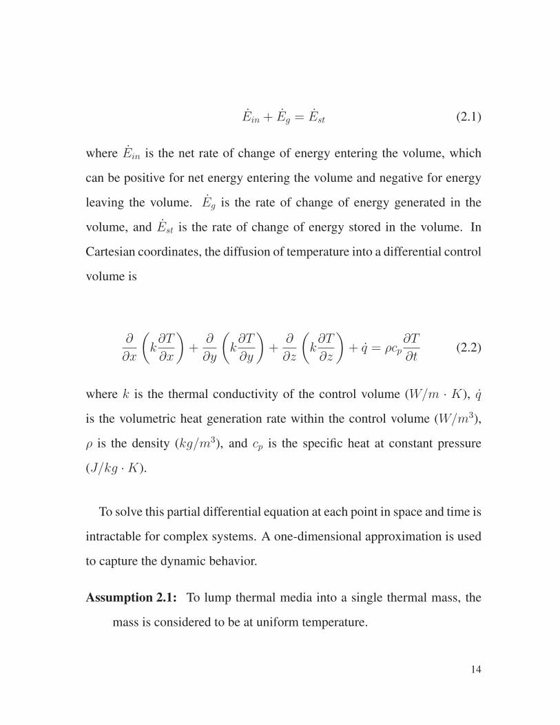
Ein + Eg = Est (2.1)
where Ein is the net rate of change of energy entering the volume, which
can be positive for net energy entering the volume and negative for energy
leaving the volume. Eg is the rate of change of energy generated in the
volume, and Est is the rate of change of energy stored in the volume. In
Cartesian coordinates, the diffusion of temperature into a differential control
volume is
∂
∂x
(
k∂T
∂x
)
+∂
∂y
(
k∂T
∂y
)
+∂
∂z
(
k∂T
∂z
)
+ q = ρcp∂T
∂t(2.2)
where k is the thermal conductivity of the control volume (W/m · K), q
is the volumetric heat generation rate within the control volume (W/m3),
ρ is the density (kg/m3), and cp is the specific heat at constant pressure
(J/kg ·K).
To solve this partial differential equation at each point in space and time is
intractable for complex systems. A one-dimensional approximation is used
to capture the dynamic behavior.
Assumption 2.1: To lump thermal media into a single thermal mass, the
mass is considered to be at uniform temperature.
14
With uniform temperature throughout the mass, the heat equation equation
simplifies to
qnet + q = ρcp∂T
∂t(2.3)
The spatial heat flow terms simplify to a net heat flow into the volume, qnet
(W). With no heat generation in the control volume, the equation is finally
reduced to
qnet = ρcp∂T
∂t(2.4)
This assumption implies that the thermal conductivity within the solid is
large when compared to the thermal conductivity between the object and its
neighboring masses or surroundings. This may make sense with an object
made of high conductivity metal, but not of thermally insulative plastic or
rubber. To model an insulative object, the mass can be discretized into many
smaller masses for better results. Composite objects like fuser rolls have to
be broken into separate masses: an object for the metal core and one or more
objects for the rubber layer.
From Incropera and DeWitt [15](pp. 76), the one-dimensional heat flow
due to conduction between two lumped masses can be represented by the
equation
15
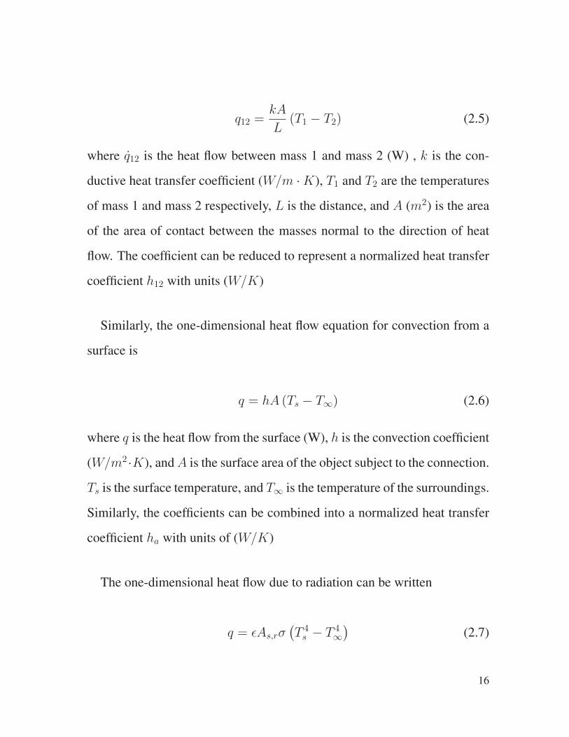
q12 =kA
L(T1 − T2) (2.5)
where q12 is the heat flow between mass 1 and mass 2 (W) , k is the con-
ductive heat transfer coefficient (W/m ·K), T1 and T2 are the temperatures
of mass 1 and mass 2 respectively, L is the distance, and A (m2) is the area
of the area of contact between the masses normal to the direction of heat
flow. The coefficient can be reduced to represent a normalized heat transfer
coefficient h12 with units (W/K)
Similarly, the one-dimensional heat flow equation for convection from a
surface is
q = hA (Ts − T∞) (2.6)
where q is the heat flow from the surface (W), h is the convection coefficient
(W/m2 ·K), andA is the surface area of the object subject to the connection.
Ts is the surface temperature, and T∞ is the temperature of the surroundings.
Similarly, the coefficients can be combined into a normalized heat transfer
coefficient ha with units of (W/K)
The one-dimensional heat flow due to radiation can be written
q = εAs,rσ(
T 4s − T 4
∞
)
(2.7)
16
where ε is the emissivity of the object, As,r is the surface area emitting the
radiation, and σ is the Stefan-Boltzman constant (σ = 5.770 · 10−8W/m2 ·
K4). The heat transfer coefficients can be combined into hr, with units of
(W/K4).
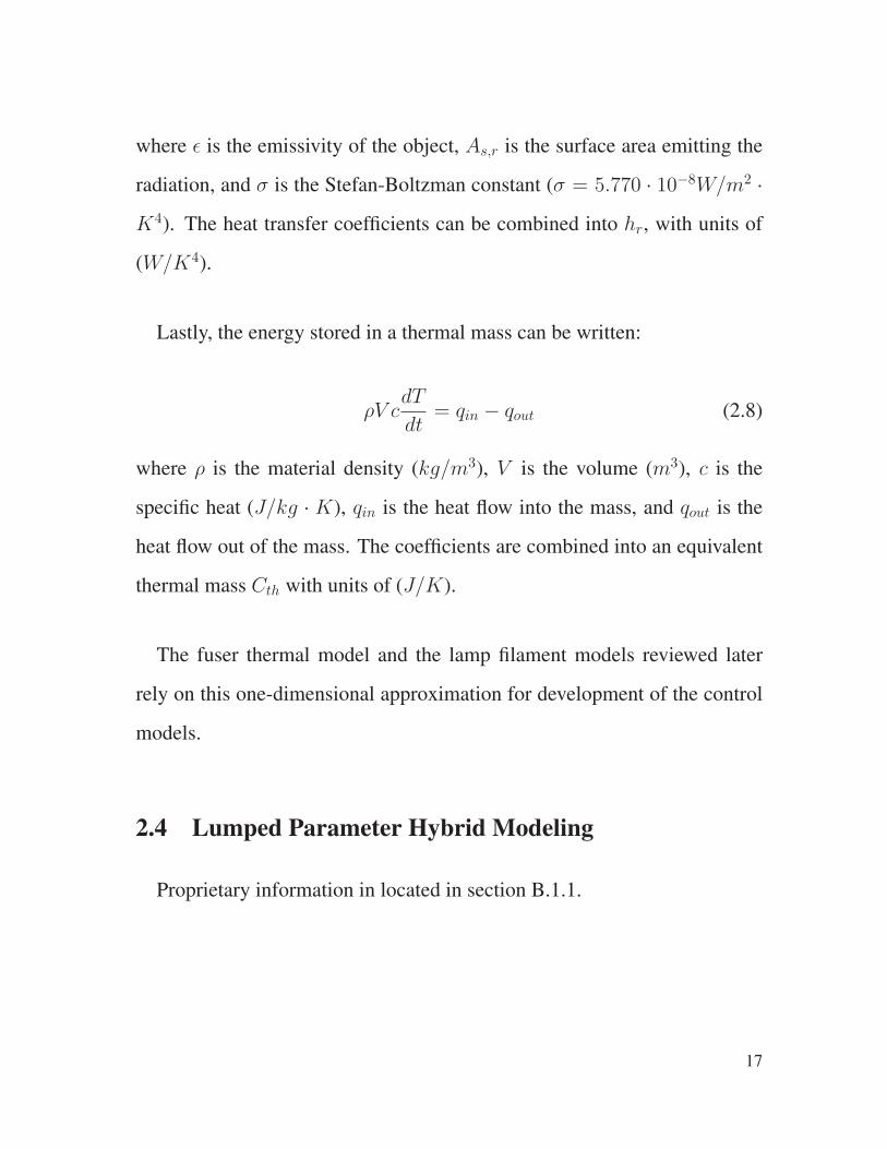
Lastly, the energy stored in a thermal mass can be written:
ρV cdT
dt= qin − qout (2.8)
where ρ is the material density (kg/m3), V is the volume (m3), c is the
specific heat (J/kg · K), qin is the heat flow into the mass, and qout is the
heat flow out of the mass. The coefficients are combined into an equivalent
thermal mass Cth with units of (J/K).
The fuser thermal model and the lamp filament models reviewed later
rely on this one-dimensional approximation for development of the control
models.
2.4 Lumped Parameter Hybrid Modeling
Proprietary information in located in section B.1.1.
17
2.5 Lamp Filament Modeling
Maeda and Takeuchi [21] developed a thermal model using a single lumped
thermal mass to represent the lamp filament in a heater for a fusing system.
Power is input to the system electrically across the resistance of the filament.
Heat power is stored or lost via convection and radiation to ambient.
Ben-Yaakov et al. [23] model a lamp filament as two lumped masses. One
mass represents the filament, the other lumps all of the remaining masses
together: the outer quartz tube, end caps, and gas inside the tube.
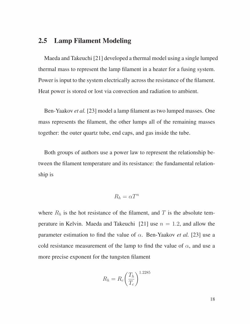
Both groups of authors use a power law to represent the relationship be-
tween the filament temperature and its resistance: the fundamental relation-
ship is
Rh = αT n
where Rh is the hot resistance of the filament, and T is the absolute tem-
perature in Kelvin. Maeda and Takeuchi [21] use n = 1.2, and allow the
parameter estimation to find the value of α. Ben-Yaakov et al. [23] use a
cold resistance measurement of the lamp to find the value of α, and use a
more precise exponent for the tungsten filament
Rh = Rc
(
Th
Tc
)1.2285
18

where Rc is the cold resistance of the filament , Tc is the absolute tempera-
ture that the cold resistance measurement was taken.
This relationship indicates that the filament resistance increases with in-
creasing temperature. The lower resistance at room temperature will cause
a high inrush current until the lamp heats up to its steady state temperature
of 1,000 to 2,000 degrees.
2.6 Power Line Flicker
The flicker of lighting systems is due to fluctuations of the power supply
voltage. Lighting fluctuations can be irritating to users of the machine, and
even induce epileptic seizures to those who are susceptible. Any electri-
cal device plugged into the power supply has the potential to cause voltage
fluctuations. This is due to the line impedance between the power supply
and the equipment. Instantaneously switching a load into the network will
cause the line voltage to drop. The IEC has enacted regulations [3] to limit
the effect of load changes of an electrical device on the power system. The
standards were developed to minimize the human perception of flicker.
The standard dictates that the evaluation of flicker is done under specific
test conditions. Mains voltages can vary from 187 Volts to 264 Volts. Flicker
is evaluated at specific values of 230 Volts at 50 Hz. Specific reference
19

j XNRN
j XARA
RL
G
M
L1
N
Figure 2.6: Example flicker circuit with reference impedances, adapted from [3]. Note that
only one phase line is shown and impedances contain a resistive part and a reactive part.
impedances are defined as the line impedance is dependent on the wiring
between the outlet in the wall and the distant power source. Figure 2.6
shows the configuration of circuit elements. G is the source voltage, M is
the voltage measuring equipment, and RL is the load resistance.
In their combined thermal and electric model, Maeda and Takeuchi [21]
represent the reference impedances as an equivalent resistor and inductor.
This is shown in figure 2.7, a switch allows the heating lamp to be connected
to the circuit.
Limits are placed on the change in RMS value of successive half-cycles
of the supply voltage. These are explicitly called out, and relatively easy
to measure. The more difficult standard to apply is the short and long-term
flicker indicator. This requires actual measurements on the equipment under
test with a device called a flickermeter.
20

Rh
Vs V(t)
230 VAC
50 Hz
Heater
I(t)
Power distribution system Fuser
LSRS
Figure 2.7: Power distribution with equivalent resistance and inductance for evaluation of
flicker with a heating lamp. Source: Maeda and Takeuchi [21].
As defined by the standard [4], a flickermeter simulates the human eye-
brain response to a 60 Watt reference lamp on a 230 Volt 50 Hz power
system. The line voltage is passed through many stages of filters to generate
the instantaneous sensation of flicker S(t).
The flicker sensitivity weighting filter, which is shown in figure 2.8, was
expressed in transfer function form in [5]. The human eye-brain system has
its highest sensitivity at approximately 8.8 Hz. This curve was determined
empirically by determining the median threshold of perceptibility at each
frequency for a group of test subjects.
The instantaneous flicker sensation S(t) is sampled and recorded. The
flicker level is evaluated statistically for different observation periods. The
short-term flicker indicator Pst is evaluated for ten minutes, the long-term
flicker indicator Plt is evaluated for two hours.
21

0 5 10 15 20 25 30 350
0.1
0.2
0.3
0.4
0.5
0.6
0.7
0.8
0.9
1
Frequency (Hz)
Magnitude
Figure 2.8: The human eye weighting filter for flicker perceptibility, using the transfer
function from [5]
The easiest method of evaluating compliance is measuring the flicker
sensation with a flickermeter and reference impedances. Determining the
flicker sensation analytically is difficult for certain cases. There are many
examples in the literature of numerically replicating the filters and signal
processing of the flickermeter. A Matlab compatible flickermeter is detailed
well by Berlola et al. [5]. However, there are many nuances in the signal
processing to eliminate filter transients at the start of the simulations. For
this work, an open-source Matlab flickermeter simulator by Jourdan [16] is
used to evaluate short-term flicker. Standard IEC test cases are provided
22

which demonstrate that the simulator meets the 5% tolerance on the calcu-
lation of Pst.
Using Matlab to simulate flicker response with a lamp filament heated
fuser system is detailed by Maeda and Takeuchi [21]. Their work demon-
strated that the simulated Pst matched their measured flickermeter readings
for various periods with a 12.5% duty cycle. Incidentally, the Pst exceeded
the limit of 1 for the periods tested.
2.7 Fuser Power Controller
The fuser power controller works by modulating the power to the lamp to
meet the flicker constraints. This is done with a high speed switching power
supply. Proprietary information is located in section B.1.2.
A similar method to modulate power to a fusing lamp is detailed by
Hirst [14]. The patent details a similar circuit to the fuser power controller.
A least mean squares (LMS) adaptive filter is used for temperature control.
2.8 Multiple Time Scales
When analyzing the thermal response and power losses of insulated gate
bipolar transistor (IGBT) switching, the problem of disparate time scales
23

arises. Zhou, et al. [27] are able to simulate the thermal behavior of the
IGBT by creating a two-dimensional lookup table from high fidelity models
for the power loss for short time scales. The authors make the assumption
that the time constant of the load is very large compared with the time con-
stant of the PWMwaveforms. This also says that current through the load is
constant over one PWM switching cycle. Determining the effective perfor-
mance at short time scales allows the simulation of a model with large time
steps for quicker iteration and longer time durations.
Using the fact that the line voltage is periodic, there is an opportunity
for using average values to approximate the fast system. As detailed by
Khalil [17] (pp. 412), perturbation theory can be used to find the average of
a system. With the linear system
x = εA(t)x (2.9)
where A(t + T ) = A(t) and ε > 0, if the average of the matrix A over the
time interval T is
A =1
T
∫ T
0
A(τ)dτ (2.10)
then the averaged system is given by
xav = εAxav (2.11)
24
The fast system can be shown to meet the criteria that A(t+T ) = A(t) if
it is periodic over the time interval τ . The slow system will meet the same
criteria if it is shown to be constant over the time interval τ .
2.9 Variational Calculus Approach to Optimal Control
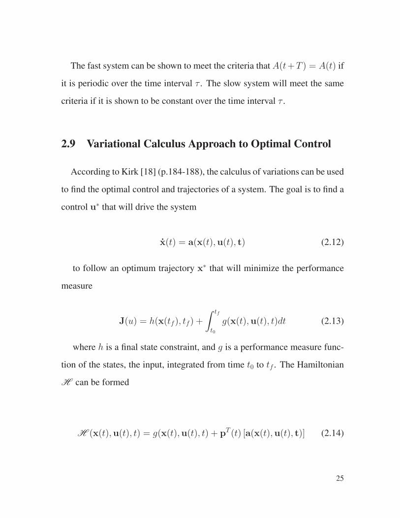
According to Kirk [18] (p.184-188), the calculus of variations can be used
to find the optimal control and trajectories of a system. The goal is to find a
control u∗ that will drive the system
x(t) = a(x(t),u(t), t) (2.12)
to follow an optimum trajectory x∗ that will minimize the performance
measure
J(u) = h(x(tf), tf) +
∫ tf
t0
g(x(t),u(t), t)dt (2.13)
where h is a final state constraint, and g is a performance measure func-
tion of the states, the input, integrated from time t0 to tf . The Hamiltonian
H can be formed
H (x(t),u(t), t) = g(x(t),u(t), t) + pT (t) [a(x(t),u(t), t)] (2.14)
25
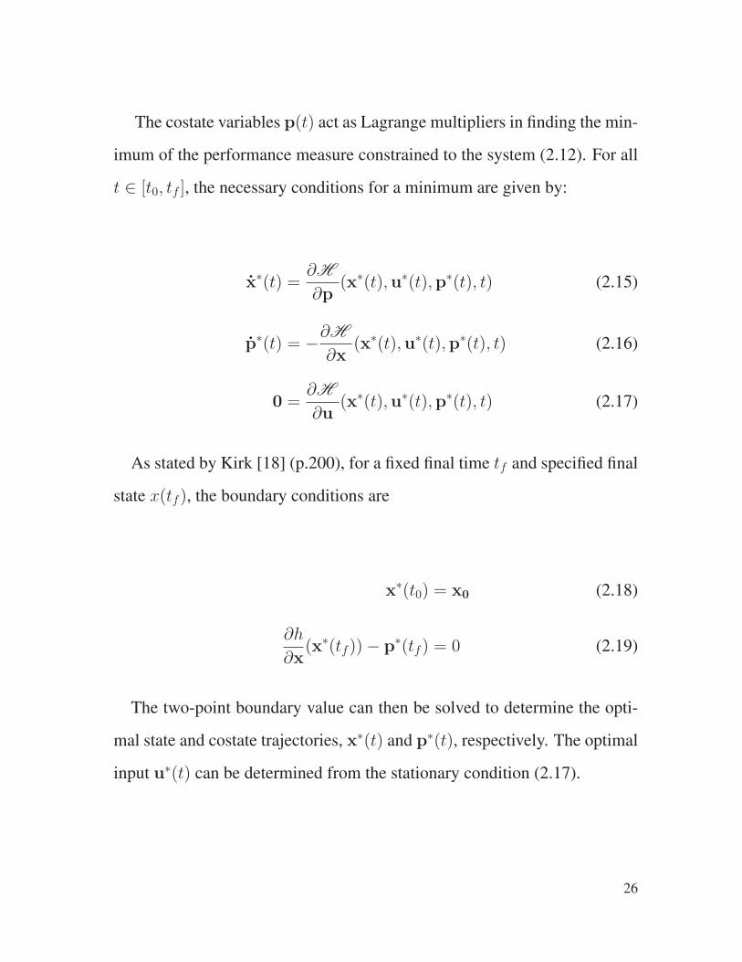
The costate variables p(t) act as Lagrange multipliers in finding the min-
imum of the performance measure constrained to the system (2.12). For all
t ∈ [t0, tf ], the necessary conditions for a minimum are given by:
x∗(t) =∂H
∂p(x∗(t),u∗(t),p∗(t), t) (2.15)
p∗(t) = −∂H
∂x(x∗(t),u∗(t),p∗(t), t) (2.16)
0 =∂H
∂u(x∗(t),u∗(t),p∗(t), t) (2.17)
As stated by Kirk [18] (p.200), for a fixed final time tf and specified final
state x(tf), the boundary conditions are
x∗(t0) = x0 (2.18)
∂h
∂x(x∗(tf))− p∗(tf) = 0 (2.19)
The two-point boundary value can then be solved to determine the opti-
mal state and costate trajectories, x∗(t) and p∗(t), respectively. The optimal
input u∗(t) can be determined from the stationary condition (2.17).
26

However, the system being considered is subject to saturation constraints
on the input. Negative power cannot be applied to the lamps, and there is
an upper limit to a lamp’s power. Pontryagin’s minimum principle can be
applied to find the optimal control with constrained input. With Pontryagin’s
minimum principle, the minimum value ofH may not be at the stationary
point described in (2.17).
As detailed by Kirk [18] (p233), when the input in constrained, the min-
imum of the Hamiltonian may not be where the partial derivative is zero.
The optimum value of the input has to be calculated explicitly with the con-
straints applied. The stationary condition (2.17) can be replaced with the
more general constraint
∂H
∂u(x∗(t),u∗(t),p∗(t), t) ≤
∂H
∂u(x∗(t),u(t),p∗(t), t) (2.20)
to find the optimal u∗(t) for all admissible u(t).
2.10 State Feedback Control
As described by Lewis and Syrmos [19], a linear quadratic regulator
drives the states of a system to zero. For a infinite-time linear system de-
scribed by
27

x = Ax+Bu (2.21)
with cost functional defined as
J =
∫ ∞
0
(
xTQx+ uTRu)
dt (2.22)
the feedback control law that minimizes the cost is given by
u = −Kx (2.23)
where the constant gain matrixK is defined as
K = R−1BTS (2.24)
and S is found by solving the continuous time algebraic Riccati equation
0 = ATS + SA− SBR−1BTS +Q (2.25)
28
Chapter 3
Fuser thermal model development
From late 2006 to early 2007, a redesign activity began on the fuser power
controller (or “Flicker Board”). This provided an opportunity to look at the
fuser temperature control and provide feedback to the electrical design. This
provided the motivation to develop a temperature control model for the Nu-
vera system. Chuck Facchini and I from the Nuvera fusing team worked
under guidance from Yongsoon Eun and Eric Hamby from the Xerox Inno-
vation Group, the Research division within Xerox.
The energy balance equations are detailed in section 3.1, and the model-
ing assumptions are reviewed in section 3.2
The experiment to capture the estimation and validation data is detailed
in section 3.3. The parameter estimation and the model fit is explained in
sections 3.4 and 3.5.
29

The initial model only included one paper type in the estimation step.
As part of this work, the model is extended in section 5.1 to encompass
the worst-case thermal loading condition. The resulting system models are
examined in section 3.6.
3.1 Energy Balance Equations
Using assumption 2.1, the three-dimensional geometry of the system will
be discretized into interconnected thermal masses.
The fuser roll is modeled as a composite object with two lumped masses.
An inner aluminum corem11, is most of the mass. A thin, highly insulative
non-stick coating forms the outer layer m12. Heat can be added to the core
through the heating lamp. The outer surface can transfer heat to the ambient
air, the pressure roll, and to the substrate.
The pressure roll is modeled as an object with two lumped masses, with
an inner steel core m22, and an outer layer of rubber m21. The pressure roll
can transfer heat from its outer surface only. Heat can be transfered to the
ambient air, the fuser roll, or to the substrate.
Separate systems of equations are used to model each of the dynamic
modes from figure 2.4. When switching modes, The temperature state vari-
ables do not change, only the heat transfer coefficients between the masses.
30
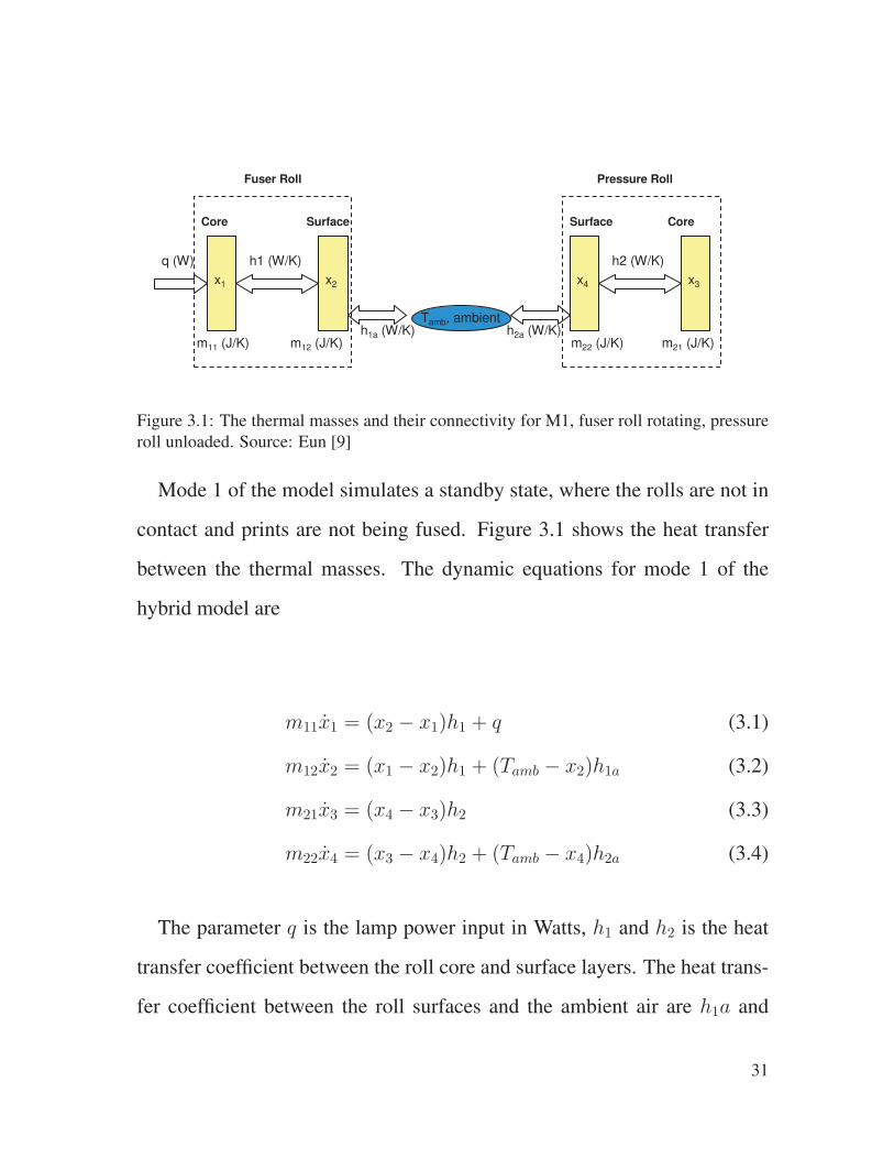
m11 (J/K) m12 (J/K)h2a (W/K)
h1 (W/K)q (W)
Tamb, ambient
x1 x2
Fuser Roll
Surface
m22 (J/K) m21 (J/K)
h2 (W/K)
x4 x3
Pressure Roll
h1a (W/K)
Core Surface Core
Figure 3.1: The thermal masses and their connectivity for M1, fuser roll rotating, pressure
roll unloaded. Source: Eun [9]
Mode 1 of the model simulates a standby state, where the rolls are not in
contact and prints are not being fused. Figure 3.1 shows the heat transfer
between the thermal masses. The dynamic equations for mode 1 of the
hybrid model are
m11x1 = (x2 − x1)h1 + q (3.1)
m12x2 = (x1 − x2)h1 + (Tamb − x2)h1a (3.2)
m21x3 = (x4 − x3)h2 (3.3)
m22x4 = (x3 − x4)h2 + (Tamb − x4)h2a (3.4)
The parameter q is the lamp power input in Watts, h1 and h2 is the heat
transfer coefficient between the roll core and surface layers. The heat trans-
fer coefficient between the roll surfaces and the ambient air are h1a and
31
h2a.
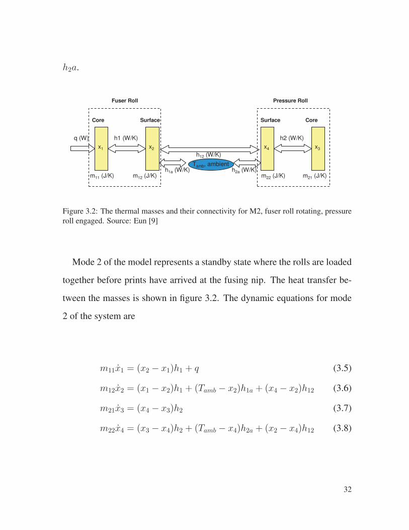
m11 (J/K) m12 (J/K)h2a (W/K)
h1 (W/K)q (W)
Tamb, ambient
x1 x2
Fuser Roll
Surface
m22 (J/K) m21 (J/K)
h2 (W/K)
x4 x3
Pressure Roll
h1a (W/K)
Core Surface Core
h12 (W/K)
Figure 3.2: The thermal masses and their connectivity for M2, fuser roll rotating, pressure
roll engaged. Source: Eun [9]
Mode 2 of the model represents a standby state where the rolls are loaded
together before prints have arrived at the fusing nip. The heat transfer be-
tween the masses is shown in figure 3.2. The dynamic equations for mode
2 of the system are
m11x1 = (x2 − x1)h1 + q (3.5)
m12x2 = (x1 − x2)h1 + (Tamb − x2)h1a + (x4 − x2)h12 (3.6)
m21x3 = (x4 − x3)h2 (3.7)
m22x4 = (x3 − x4)h2 + (Tamb − x4)h2a + (x2 − x4)h12 (3.8)
32
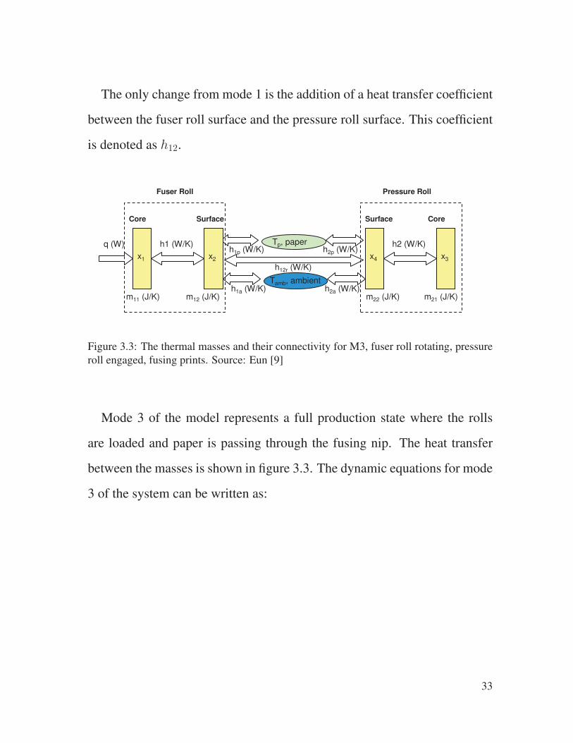
The only change from mode 1 is the addition of a heat transfer coefficient
between the fuser roll surface and the pressure roll surface. This coefficient
is denoted as h12.
h12r (W/K)
h2p (W/K)h1p (W/K)Tp, paper
m11 (J/K) m12 (J/K)h2a (W/K)
h1 (W/K)q (W)
Tamb, ambient
x1 x2
Fuser Roll
Surface
m22 (J/K) m21 (J/K)
h2 (W/K)
x4 x3
Pressure Roll
h1a (W/K)
Core Surface Core
Figure 3.3: The thermal masses and their connectivity for M3, fuser roll rotating, pressure
roll engaged, fusing prints. Source: Eun [9]
Mode 3 of the model represents a full production state where the rolls
are loaded and paper is passing through the fusing nip. The heat transfer
between the masses is shown in figure 3.3. The dynamic equations for mode
3 of the system can be written as:
33
m11x1 = (x2 − x1)h1 + q (3.9)
m12x2 = (x1 − x2)h1 + (Tamb − x2)h1a + (x4 − x2)h12r
+ (Tp − x2)h1p
(3.10)
m21x3 = (x4 − x3)h2 (3.11)
m22x4 = (x3 − x4)h2 + (Tamb − x4)h2a + (x2 − x4)h12r
+ (Tp − x4)h2p
(3.12)
Note that h12r in (3.10) and (3.12) is a heat transfer coefficient between
the fuser and pressure rolls specific to the run condition.
3.2 Assumptions
The objective of this model is to capture the dynamics at the temperature
sensor feedback location. The fuser roll surface temperature is the system
output which the image quality metrics are derived. This model is valid
under the following assumptions.
Assumption 3.1: The temperature of each thermal mass in the model is
uniform.
This is the same as assumption 2.1, which allows the one dimensional analy-
sis and use the concept of thermal resistance between lumped masses. This
34
is valid when the temperature gradients within each mass are small. Be-
cause of the low conductivity of the silicone rubber on the pressure roll,
the temperature is not uniform within the material, violating assumption
3.1. However, capturing the fuser roll surface temperature is the goal, so
the bulk temperature of the pressure roll may be sufficient to capture the
dynamics of interest. The temperature of the mass will be measured at the
center of paper.
Assumption 3.2: The electrical power applied to the heating lamp is con-
verted into thermal heat with 100% efficiency and applied to the fuser
roll core instantaneously.
Considering that the fuser roll is relatively high mass, the lag associated
with applying power to the lamp is small compared to the thermal response
of the system. The fuser may take four minutes to warm up to the operating
temperature. The lag in heat power may be significant with an “instant on”
product where the thermal mass is low and the warm up time is less than 30
seconds.
Assumption 3.3: The ambient temperature is constant, at 25 C.
To derive convective heat transfer coefficients in (2.6), the ambient temper-
ature must be known. In reality, the ambient temperature inside the machine
near the fuser will increase as the machine runs. For a more precise model,
machine cavity temperature would became a state in the system model.
35
Assumption 3.4: The thermal load of the paper can be represented by con-
tact losses to a solid at room temperature of 25 C.
When printing, the fuser sees a constant stream of paper entering at room
temperature. This would not be applicable when printing duplex, where the
paper will retain heat from fusing side one, and be above room temperature
when side two is fused.
Assumption 3.5: The model is only applicable for the specific paper type
tested, both in length and width, pitch, and print rate.
The thermal contact resistance of the paper is part of the system model. A
new set of heat transfer coefficients has to be determined for each different
paper type run.
Assumption 3.6: The ambient heat transfer to and from the fuser roll is
valid when the roll is spinning.
The heat transfer coefficients will be different with a stationary roll. The
power required to keep the spinning roll at temperature will be higher with
the roll spinning.
Assumption 3.7: The thermistor assemblies measuring the temperature have
a 4 second time constant
The soft-touch thermistors have a thermistor chip bonded to a small metal
plate, with a layer of PTFE tape on top. The sensor time constant will in-
crease and pick up steady state error as sensors become contaminated with
36
toner and paper dust. This inaccuracy was avoided by cleaning the thermis-
tor surfaces before testing, and running the required media with no image.
3.3 Experimental Setup
To develop the thermal model, a Nuvera fuser had to be instrumented
with additional temperature sensors as it ran inside a machine. In the Nu-
vera machine, only the surface temperature of the fuser roll is measured.
The remaining states have to be measured in order to fit the model. The
thermistors used to measure surface temperature are the same used in pro-
duction, and have a time constant of about 4 seconds.
A strip of topcoat was removed from the fuser roll to allow the aluminum
core to be exposed. This allowed a soft-touch thermistor to be placed on
the core to measure the temperature. A thermistor in the standard center
location measured the surface temperature. A view of the paper entrance
side of the fuser roll assembly is shown in figure 3.4.
A thermistor was easily placed on the surface of the pressure roll. To
measure the temperature of the steel core, a thermocouple was placed inside
a soft-touch thermistor housing. This assembly was positioned to contact
the inside of the hollow core as it rotated, attached to a center support shaft.
The instrumented pressure roll is shown in figure 3.5.
37
Figure 3.4: Experimental setup with temperature sensors on fuser roll. Source: C. Fac-
chini [9]
Because the testing may take the fuser temperatures outside their normal
ranges, a slave fuser was placed outside the machine. This slave had the
normal lamp inputs and temperature signals connected to the Nuvera ma-
chine. This allowed the machine to heat the slave fuser and measure healthy
temperature signals to keep the temperature fault detection algorithms from
shutting down the machine.
The instrumented fuser was connected to the rest of the machine controls.
This allowed the instrumented fuser to be controlled normally to pass paper
38
Figure 3.5: Experimental setup with temperature sensors on the pressure roll. Source: C.
Facchini [9]
through it.
A separate power relay was set up to provide power to the lamp. The duty
cycle was adjusted to modulate the lamp power levels. The temperature
signals from the instrumented fuser were acquired by an Agilent 34970A
data acquisition switch unit.
39
3.4 Parameter Estimation - Step 1
The parameter optimization was done in two stages, the first derived the
parameters for modes M1 and M2, previously defined in section 3.1. Two
runs of data were collected, one for parameter estimation, and one for vali-
dation. The same ”flight plan” was used in both cases:
1. 2200 watts was applied to the lamp to bring the fuser up to the operat-
ing range
2. The power was reduced to 206 watts
3. The pressure roll was loaded into the fuser roll
The model parameters were optimized using the “fminsearch” function in
Matlab [2]. The performance index used was the integral of the square of the
error between the measured states and the model states. The optimal values
of the parameters are shown in table B.1. The model performance is shown
in figure 3.6. The pressure roll surface temperature, x4 shows poor agree-
ment. This could be because of the poor conductivity of the pressure roll
rubber and it’s thickness. Liu [20] used many states within a rubber layer
with poor conductivity; more layers could be added to improve tracking of
this state.
The model using the validation set shows good tracking.
40
0 60 120 180 240 300 360 420 480 540 600 660 720 7800
50
100
150
200
250
Time (s)
Tem
pera
ture
(°C
)
loading1
x1
x2
x3
x4
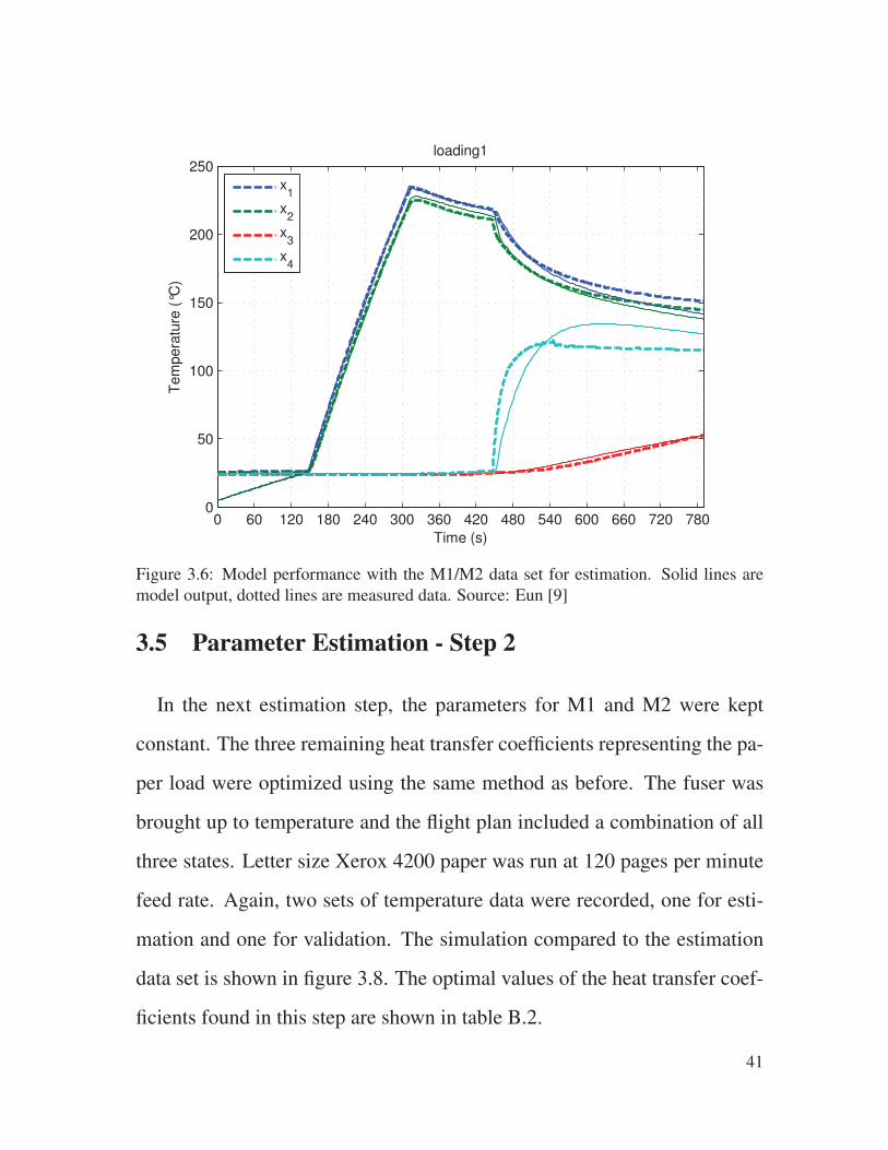
Figure 3.6: Model performance with the M1/M2 data set for estimation. Solid lines are
model output, dotted lines are measured data. Source: Eun [9]
3.5 Parameter Estimation - Step 2
In the next estimation step, the parameters for M1 and M2 were kept
constant. The three remaining heat transfer coefficients representing the pa-
per load were optimized using the same method as before. The fuser was
brought up to temperature and the flight plan included a combination of all
three states. Letter size Xerox 4200 paper was run at 120 pages per minute
feed rate. Again, two sets of temperature data were recorded, one for esti-
mation and one for validation. The simulation compared to the estimation
data set is shown in figure 3.8. The optimal values of the heat transfer coef-
ficients found in this step are shown in table B.2.
41

0 60 120 180 240 300 36060
80
100
120
140
160
180
200
220
240
Time (s)
Tem
pera
ture
(°C
)
loading 2
x1
x2
x3
x4
Figure 3.7: Model performance with the M1/M2 data set for validation. Solid lines are
model output, dotted lines are measured data. Source: Eun [9]
The model showed good tracking with the validation data set in figure
3.9. However, the high frequency content of the fuser roll transients at t =
300 and t = 600 are not captured. This could be due to the low thermal
conductivity of the fuser roll coating, similar to [20].
The model fit can be quantified by calculating the R2 value in the same
fashion as a linear regression. In (3.13), xi are the observed values, xi is
the estimate from the model, and x is the mean of the observed data. In this
case the error in the R2 calculation represents the unexplained variance and
will contain lack-of-fit error as well as measurement error.
42
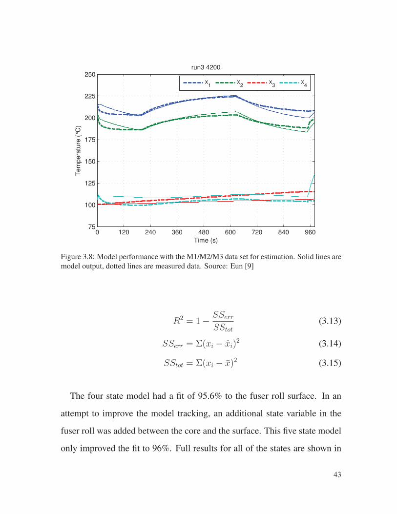
0 120 240 360 480 600 720 840 96075
100
125
150
175
200
225
250
Time (s)
Tem
pera
ture
(°C
)
run3 4200
x
1x
2x
3x
4
Figure 3.8: Model performance with the M1/M2/M3 data set for estimation. Solid lines are
model output, dotted lines are measured data. Source: Eun [9]
R2 = 1−SSerr
SStot
(3.13)
SSerr = Σ(xi − xi)2 (3.14)
SStot = Σ(xi − x)2 (3.15)
The four state model had a fit of 95.6% to the fuser roll surface. In an
attempt to improve the model tracking, an additional state variable in the
fuser roll was added between the core and the surface. This five state model
only improved the fit to 96%. Full results for all of the states are shown in
43
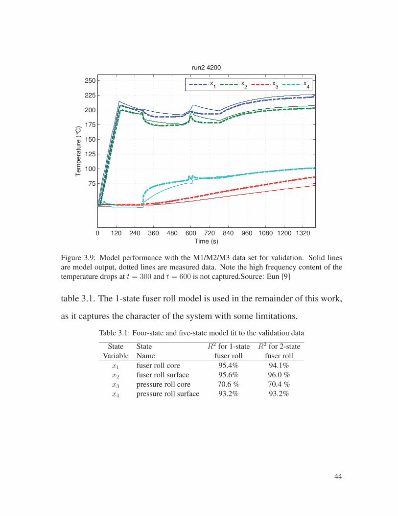
0 120 240 360 480 600 720 840 960 1080 1200 1320
75
100
125
150
175
200
225
250
Time (s)
Tem
pera
ture
(°C
)
run2 4200
x1
x2
x3
x4
Figure 3.9: Model performance with the M1/M2/M3 data set for validation. Solid lines
are model output, dotted lines are measured data. Note the high frequency content of the
temperature drops at t = 300 and t = 600 is not captured.Source: Eun [9]
table 3.1. The 1-state fuser roll model is used in the remainder of this work,
as it captures the character of the system with some limitations.
Table 3.1: Four-state and five-state model fit to the validation data
State State R2 for 1-state R2 for 2-state
Variable Name fuser roll fuser roll
x1 fuser roll core 95.4% 94.1%
x2 fuser roll surface 95.6% 96.0 %
x3 pressure roll core 70.6 % 70.4 %
x4 pressure roll surface 93.2% 93.2%
44
3.6 Discussion
This model’s utility is limited as it is only valid for the thermal load of one
media type. To estimate the heat transfer coefficients for additional paper
types, additional data has to be gathered. This involves more open loop ex-
periments along with repetition of the parameter optimization process from
section 3.5. A method to extend this model will be addressed in chapter 5.
At approximately t = 300s and t = 600 s in figure 3.9, there is a fast
drop in temperature that is not captured by the model. The addition of a
state in the fuser roll did not improve the the model performance. With
assumption 3.1, many masses of uniform temperature may be needed to
capture the steep gradients in the system. Additional delays and states could
be added as in [20] to remove error.
45

Chapter 4
Problem Statement
There are many examples in the literature of lumped thermal analysis
of fusing systems and lamp filaments. The simulation and design of the
power switching system has been extensive to mitigate electrical transients.
However, the integrated system has not yet been assembled or analyzed to
determine the limits of performance. One of the issues with this integrated
model is bridging the gap between the fast switching dynamics and the slow
thermal dynamics. The goal of this work is to understand the interactions
between the thermal and electrical systems, with the primary goal of im-
proving temperature control performance subject to flicker constraints.
1. Starting with the existing thermal model described in chapter 3, iden-
tify the dynamics of the heating lamp and power system to capture the
worst-case start up droop behavior and demonstrate performance of
this complete model.
2. Formulate the open-loop optimal control problem, and find the limits
46

of performance of the system with the current startup sequence.
3. Using the open-loop optimal control problem, find the optimum timing
for the startup sequence.
4. Design a controller to reduce the droop transient performance to ±
[information redacted] C based on the worst-case thermal load using
the integrated model, or determine the limits of performance.
Startup droop is inherent in most fusing systems, flicker constraints will
reduce the performance if not considered in the control design. It is the hope
that the integrated approach to this thermo-electric system will guide future
engineers in designing the temperature control systems and the architecture
of future products.
Note: The complete problem statement is located in appendix B.3
47
Chapter 5
Fuser thermal model refinement
The model developed in chapter 3 was for only one specific paper type.
The system response is highly sensitive to the heat transfer coefficients be-
tween the paper and the rollers. Temperature transients are amplified when
the thermal load is high. The lamp is also closer to saturation with a higher
paper load, there is not much headroom to increase power. In section 5.1,
the thermal model is refined to incorporate different paper loads.
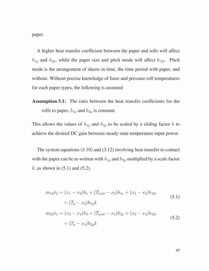
5.1 Thermal load sliding factor
The fact that the plant model contains the thermal conductivity between
the rolls and the paper will create difficulties when trying to design a con-
troller. A controller can be designed to work well with the one particular pa-
per, but will degrade in performance as the paper properties change. Coated
stocks will have a higher heat transfer coefficient than uncoated substrates.
Historical data is available showing steady state power required for a given
48
paper.
A higher heat transfer coefficient between the paper and rolls will affect
h1p and h2p, while the paper size and pitch mode will affect h12r. Pitch
mode is the arrangement of sheets in time, the time period with paper, and
without. Without precise knowledge of fuser and pressure roll temperatures
for each paper types, the following is assumed
Assumption 5.1: The ratio between the heat transfer coefficients for the
rolls to paper, h1p and h2p is constant.
This allows the values of h1p and h2p to be scaled by a sliding factor k to
achieve the desired DC gain between steady state temperature input power.
The system equations (3.10) and (3.12) involving heat transfer to contact
with the paper can be re-written with h1p and h2p multiplied by a scale factor
k, as shown in (5.1) and (5.2).
m12x2 = (x1 − x2)h1 + (Tamb − x2)h1a + (x4 − x2)h12r
+ (Tp − x2)h1pk(5.1)
m22x4 = (x3 − x4)h2 + (Tamb − x4)h2a + (x2 − x4)h12r
+ (Tp − x4)h2pk(5.2)
49

Some further manipulation is required to find the relationship between
k and the dc gain of the system. The systems of equations for all three
dynamic modes can be represented in state-space form
x =
A1x+Bu+W1d for M1
A2x+Bu+W1d for M2
A3x+Bu+W2d for M3
(5.3)
Where
x =
x1
x2
x3
x4
u = [q] d =
Tamb
Tpaper
(5.4)
A1 =
−h1
m11
h1
m11
0 0
h1
m12
−h1+h1a
m12
0 0
0 0 −h2
m21
h2
m21
0 0 h2
m22
−h12+h2a
m22
(5.5)
A2 =
−h1
m11
h1
m11
0 0
h1
m12
−h1+h1a+h12
m12
0 h12
m12
0 0 −h2
m21
h2
m21
0 h12
m22
h2
m22
−h12+h2a
m22
(5.6)
50
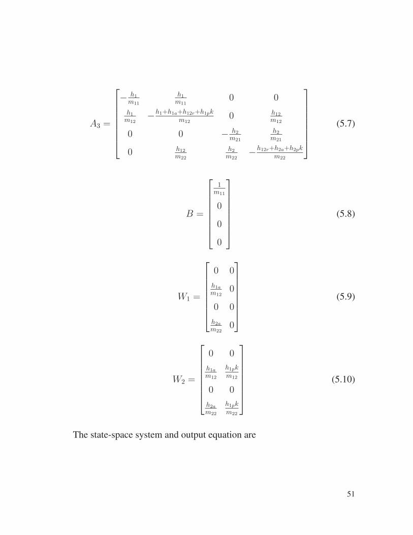
A3 =
−h1
m11
h1
m11
0 0
h1
m12
−h1+h1a+h12r+h1pk
m12
0 h12
m12
0 0 −h2
m21
h2
m21
0 h12
m22
h2
m22
−h12r+h2a+h2pk
m22
(5.7)
B =
1
m11
0
0
0
(5.8)
W1 =
0 0
h1a
m12
0
0 0
h2a
m22
0
(5.9)
W2 =
0 0
h1a
m12
h1pk
m12
0 0
h2a
m22
h1pk
m22
(5.10)
The state-space system and output equation are
51

x = Aix+Bu+Wjd (5.11)
y = Cx (5.12)
where i and j are set according to the dynamic mode, and the output equa-
tion extracts the fuser roll surface temperature
C =[
0 1 0 0]
(5.13)
for any mode at steady-state, the state derivatives are zero
0 = Aix+Bu+Wjd (5.14)
y = Cx (5.15)
Rearranging 5.14 and substituting 5.15, the relationship between the fuser
roll temperature and the power input can be found
y + CAi−1Wjd = −CAi
−1Bu (5.16)
when Tamb = Tp, the disturbance term simplifies to Tamb. Any power ap-
plied to the system will raise the temperature above the ambient.
52
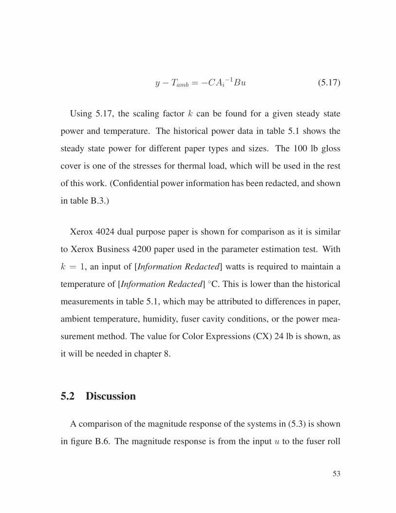
y − Tamb = −CAi−1Bu (5.17)
Using 5.17, the scaling factor k can be found for a given steady state
power and temperature. The historical power data in table 5.1 shows the
steady state power for different paper types and sizes. The 100 lb gloss
cover is one of the stresses for thermal load, which will be used in the rest
of this work. (Confidential power information has been redacted, and shown
in table B.3.)
Xerox 4024 dual purpose paper is shown for comparison as it is similar
to Xerox Business 4200 paper used in the parameter estimation test. With
k = 1, an input of [Information Redacted] watts is required to maintain a
temperature of [Information Redacted] C. This is lower than the historical
measurements in table 5.1, which may be attributed to differences in paper,
ambient temperature, humidity, fuser cavity conditions, or the power mea-
surement method. The value for Color Expressions (CX) 24 lb is shown, as
it will be needed in chapter 8.
5.2 Discussion
A comparison of the magnitude response of the systems in (5.3) is shown
in figure B.6. The magnitude response is from the input u to the fuser roll
53
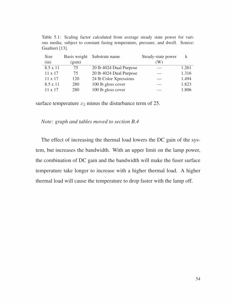
Table 5.1: Scaling factor calculated from average steady state power for vari-
ous media; subject to constant fusing temperature, pressure, and dwell. Source:
Gualtieri [13].
Size Basis weight Substrate name Steady-state power k
(in) (gsm) (W)
8.5 x 11 75 20 lb 4024 Dual Purpose — 1.261
11 x 17 75 20 lb 4024 Dual Purpose — 1.316
11 x 17 120 24 lb Color Xpressions — 1.494
8.5 x 11 280 100 lb gloss cover — 1.823
11 x 17 280 100 lb gloss cover — 1.806
surface temperature x2 minus the disturbance term of 25.
Note: graph and tables moved to section B.4
The effect of increasing the thermal load lowers the DC gain of the sys-
tem, but increases the bandwidth. With an upper limit on the lamp power,
the combination of DC gain and the bandwidth will make the fuser surface
temperature take longer to increase with a higher thermal load. A higher
thermal load will cause the temperature to drop faster with the lamp off.
54
Chapter 6
Lamp filament model development
To get an understanding of the interaction between the fuser power con-
troller and the heating lamp, a model was fit to measurements of a cold start
of the Nuvera heating lamp. In this section, the parameters for the one-state
nonlinear model detailed by Maeda and Takeuchi [21] and the two-state
lamp model detailed by Ben-Yaakov, et al. [23] will be fit.
Section 6.1 reviews the relationship between the filament temperature and
resistance. Section 6.2 reviews the lumped mass thermal equations and their
assumptions. Section 6.3 details the experiment to measure the lamp voltage
and current. The estimation of the model parameters is detailed in section
6.4.
With the estimated parameters the bandwidth of the nonlinear system is
examined in section 6.5. The comparison of the model and a standard lamp
power to voltage relationship is evaluated in 6.7. Some lamp simulations
55
and the corresponding flicker response are shown in section 6.8.
6.1 Tungsten Filament Resistance
The electrical behaviors of the model will depend on the temperature of
the tungsten filament, as the resistance of the filament increases with tem-
perature. The filament temperature cannot be measured directly and has to
be inferred from the known temperature to voltage characteristic of tung-
sten. Both lamp filament models from the literature use the same power
relationship between resistance and temperature
Rh
Rc
=
(
Th
Tc
)n
(6.1)
where Rh is the hot filament resistance (Ω), Th is the hot filament tem-
perature (K), Rc is the cold filament resistance (Ω), and Tc is the cold
filament temperature (K). An exponent (n) of 1.2 is used by Maeda and
Takeuchi [21], while an exponent of 1.2285 is used by Ben-Yaakov, et al. [23].
A value of 1.2048 is also found in the literature.
The heating lamp examined in this work is rated for 2200 watts at 208
volts RMS. A cold resistance measurement was taken using a Fluke 8842A
multimeter at 22 C. The mean resistance of 10 lamps measured 1.570 ohms
with a standard deviation of 0.029 ohms. At the operating voltage the re-
sistance is calculated by R = V 2/P , which gives R = 19.67Ω. With an
56
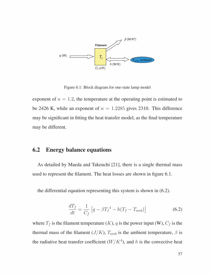
Cf (J/K)
q (W)
Tamb, ambientTf
h (W/K)
Filament
β (W/K4)
Tf
Figure 6.1: Block diagram for one-state lamp model
exponent of n = 1.2, the temperature at the operating point is estimated to
be 2426 K, while an exponent of n = 1.2285 gives 2310. This difference
may be significant in fitting the heat transfer model, as the final temperature
may be different.
6.2 Energy balance equations
As detailed by Maeda and Takeuchi [21], there is a single thermal mass
used to represent the filament. The heat losses are shown in figure 6.1.
the differential equation representing this system is shown in (6.2).
dTf
dt=
1
Cf
[
q − βTf4− h(Tf − Tamb)
]
(6.2)
where Tf is the filament temperature (K), q is the power input (W),Cf is the
thermal mass of the filament (J/K), Tamb is the ambient temperature, β is
the radiative heat transfer coefficient (W/K4), and h is the convective heat
57
transfer coefficient (W/K). This model structure assumes the following
Assumption 6.1: The lamp filament can be represented as one mass with
uniform temperature
Assumption 6.2: The heat flow from the lamp due to radiation is only a
function of filament temperature
Assumption 6.3: The heat flow from the lamp due to convection is propor-
tional to the difference between the filament and ambient temperature
Assumption 6.1 could mean either the thermal mass of the lamp casing
and the halogen gas inside are lumped into the same mass as the filament, or
the quartz casing and the gas are lumped with the surroundings. The former
may have been the author’s intent, as a halogen lamp operates at a much
higher temperature than a standard incandescent bulb.
Assumption 6.2 assumes that the filament does not absorb heat through
radiation from the ambient. The heat being absorbed by the filament is small
if T 4f T 4
amb. With the filament temperature at 2,300 K and ambient at 300
K, T 4f /T
4amb ≈ 3400 .
Assumption 6.3 assumes that the heat loss is due to the difference between
the filament temperature and ambient. The heat loss may actually be lower,
58
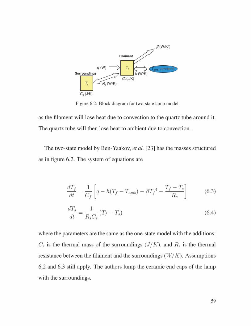
Ts
Cf (J/K)
q (W) Tamb, ambient
h (W/K)
Filament
Cs (J/K)
Surroundings
Rs (W/K)
β (W/K4)
Tf
Figure 6.2: Block diagram for two-state lamp model
as the filament will lose heat due to convection to the quartz tube around it.
The quartz tube will then lose heat to ambient due to convection.
The two-state model by Ben-Yaakov, et al. [23] has the masses structured
as in figure 6.2. The system of equations are
dTf
dt=
1
Cf
[
q − h(Tf − Tamb)− βTf4−
Tf − Ts
Rs
]
(6.3)
dTs
dt=
1
RsCs
(Tf − Ts) (6.4)
where the parameters are the same as the one-state model with the additions:
Cs is the thermal mass of the surroundings (J/K), and Rs is the thermal
resistance between the filament and the surroundings (W/K). Assumptions
6.2 and 6.3 still apply. The authors lump the ceramic end caps of the lamp
with the surroundings.
59

In both models, the electrical input power is given by
q =Vin
2
Rh
(6.5)
where Vin is the input voltage (V ), and Rh is the filament resistance (Ω).
6.3 Experimental Setup
The following were used to measure the current and voltage across the
Nuvera heating lamp:
1. Tektronix P5200 High Voltage Differential Probe
2. Tektronix TCP303 (150A DC) current probe with TCPA300 amplifier
3. Tektronix TDS3014C oscilloscope
Three phase 60Hz power chassis was used to drive the lamp. Two hot
lines of 120 V RMS, 120 apart are placed across the lamp, giving a differ-
ential voltage of 208 V.
Several measurements of the lamp starting from room ambient tempera-
ture were carried out. The data set used for estimation is shown in figure
6.3. The high inrush current causes the line voltage to drop, which is the
effect that causes flicker in lighting systems.
60
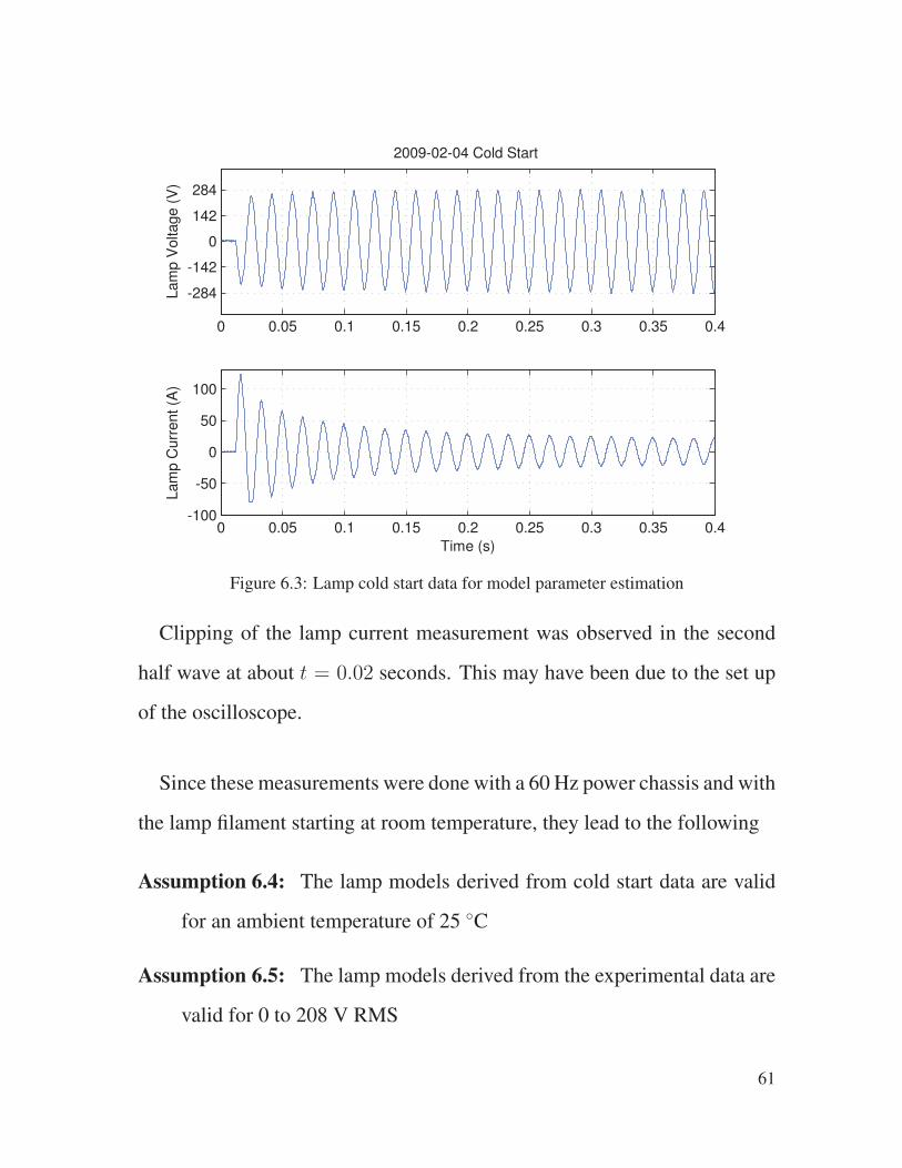
0 0.05 0.1 0.15 0.2 0.25 0.3 0.35 0.4
-284
-142
0
142
284
Lam
p V
oltage (
V)
2009-02-04 Cold Start
0 0.05 0.1 0.15 0.2 0.25 0.3 0.35 0.4-100
-50
0
50
100
Lam
p C
urr
ent (A
)
Time (s)
Figure 6.3: Lamp cold start data for model parameter estimation
Clipping of the lamp current measurement was observed in the second
half wave at about t = 0.02 seconds. This may have been due to the set up
of the oscilloscope.
Since these measurements were done with a 60 Hz power chassis and with
the lamp filament starting at room temperature, they lead to the following
Assumption 6.4: The lamp models derived from cold start data are valid
for an ambient temperature of 25 C
Assumption 6.5: The lamp models derived from the experimental data are
valid for 0 to 208 V RMS
61
Assumption 6.5 will be revisited later, as the 50 Hz system subject to flicker
constraints operates at 230 V.
6.4 Parameter Estimation
Since the cold resistance measurements were available, (6.1) will be used
for both models to relate filament temperature and resistance. The fit of the
model will only be dependent on the difference in state equations. Both
values of n in (6.1) will be fit independently. The values of the parameters
are not unique, and are highly dependent on the initial guesses.
The non-linear state equations for both models were implemented in the
Simulink tool in Matlab. The optimum parameters were found using the
fminsearch function in Matlab to minimize the quadratic cost function
J = Σ(y − y)2 (6.6)
Where y is the measured current, and y is the model estimate. The values
were constrained to be positive, and initial guesses for the heat transfer coef-
ficients were made to make the radiation term to be 99% of the total energy
loss. The optimum parameters are shown in table 6.1.
The optimal parameters for the two-state model are shown in table 6.2
62
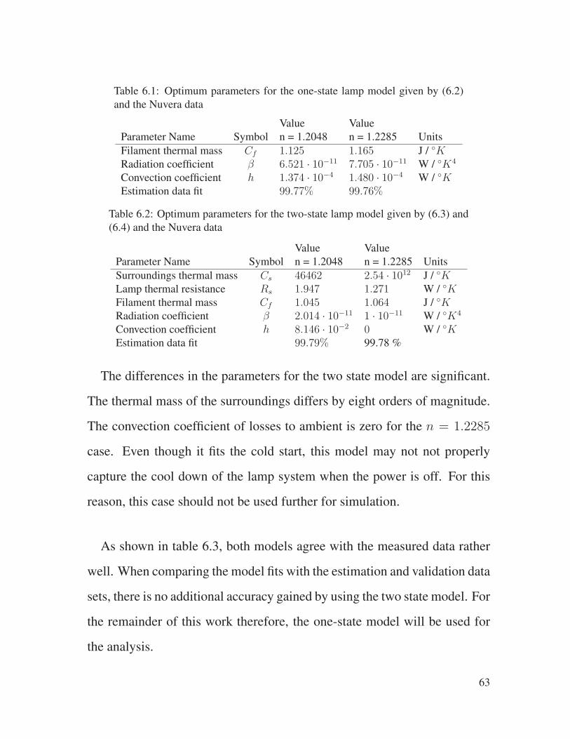
Table 6.1: Optimum parameters for the one-state lamp model given by (6.2)
and the Nuvera data
Value Value
Parameter Name Symbol n = 1.2048 n = 1.2285 Units
Filament thermal mass Cf 1.125 1.165 J / KRadiation coefficient β 6.521 · 10−11 7.705 · 10−11 W / K4
Convection coefficient h 1.374 · 10−4 1.480 · 10−4 W / KEstimation data fit 99.77% 99.76%
Table 6.2: Optimum parameters for the two-state lamp model given by (6.3) and
(6.4) and the Nuvera data
Value Value
Parameter Name Symbol n = 1.2048 n = 1.2285 Units
Surroundings thermal mass Cs 46462 2.54 · 1012 J / KLamp thermal resistance Rs 1.947 1.271 W / KFilament thermal mass Cf 1.045 1.064 J / KRadiation coefficient β 2.014 · 10−11 1 · 10−11 W / K4
Convection coefficient h 8.146 · 10−2 0 W / KEstimation data fit 99.79% 99.78 %
The differences in the parameters for the two state model are significant.
The thermal mass of the surroundings differs by eight orders of magnitude.
The convection coefficient of losses to ambient is zero for the n = 1.2285
case. Even though it fits the cold start, this model may not not properly
capture the cool down of the lamp system when the power is off. For this
reason, this case should not be used further for simulation.
As shown in table 6.3, both models agree with the measured data rather
well. When comparing the model fits with the estimation and validation data
sets, there is no additional accuracy gained by using the two state model. For
the remainder of this work therefore, the one-state model will be used for
the analysis.
63
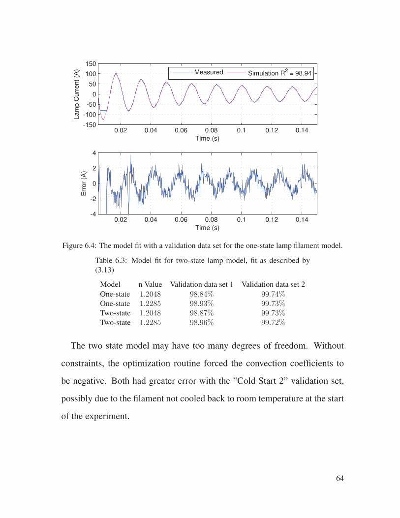
0.02 0.04 0.06 0.08 0.1 0.12 0.14-150
-100
-50
0
50
100
150
Lam
p C
urr
ent (A
)
Time (s)
Measured Simulation R2 = 98.94
0.02 0.04 0.06 0.08 0.1 0.12 0.14-4
-2
0
2
4
Err
or
(A)
Time (s)
Figure 6.4: The model fit with a validation data set for the one-state lamp filament model.
Table 6.3: Model fit for two-state lamp model, fit as described by
(3.13)
Model n Value Validation data set 1 Validation data set 2
One-state 1.2048 98.84% 99.74%One-state 1.2285 98.93% 99.73%Two-state 1.2048 98.87% 99.73%Two-state 1.2285 98.96% 99.72%
The two state model may have too many degrees of freedom. Without
constraints, the optimization routine forced the convection coefficients to
be negative. Both had greater error with the ”Cold Start 2” validation set,
possibly due to the filament not cooled back to room temperature at the start
of the experiment.
64

6.5 Bandwidth and system response
To understand the dynamic response of the non-linear system, the non-
linear system has to be linearized about an operating point as detailed by
Skogestad and Postlethwaite [24] (pp. 8) . The system in (6.2) is
Cf
dTf
dt= −βTf
4− h (Tf − Tamb) + q (6.7)
the Taylor series expansion for x4 in the neighborhood of point a is
x4 = a4 + 4a3(x− a) + 6a2(x− a)2 + 2a(x− a)3 + · · · (6.8)
discarding the second-order terms and higher and simplifying
x4 ≈ −3a4 + 4a3x (6.9)
If Tf∗ is the operating point about which that the system is being linearized,
and using (6.9), the system then becomes
Cf
dTf
dt= −β
(
−3T ∗f4 + 4T ∗f
3Tf
)
− h (Tf − Tamb) + q (6.10)
rearranging the above
65
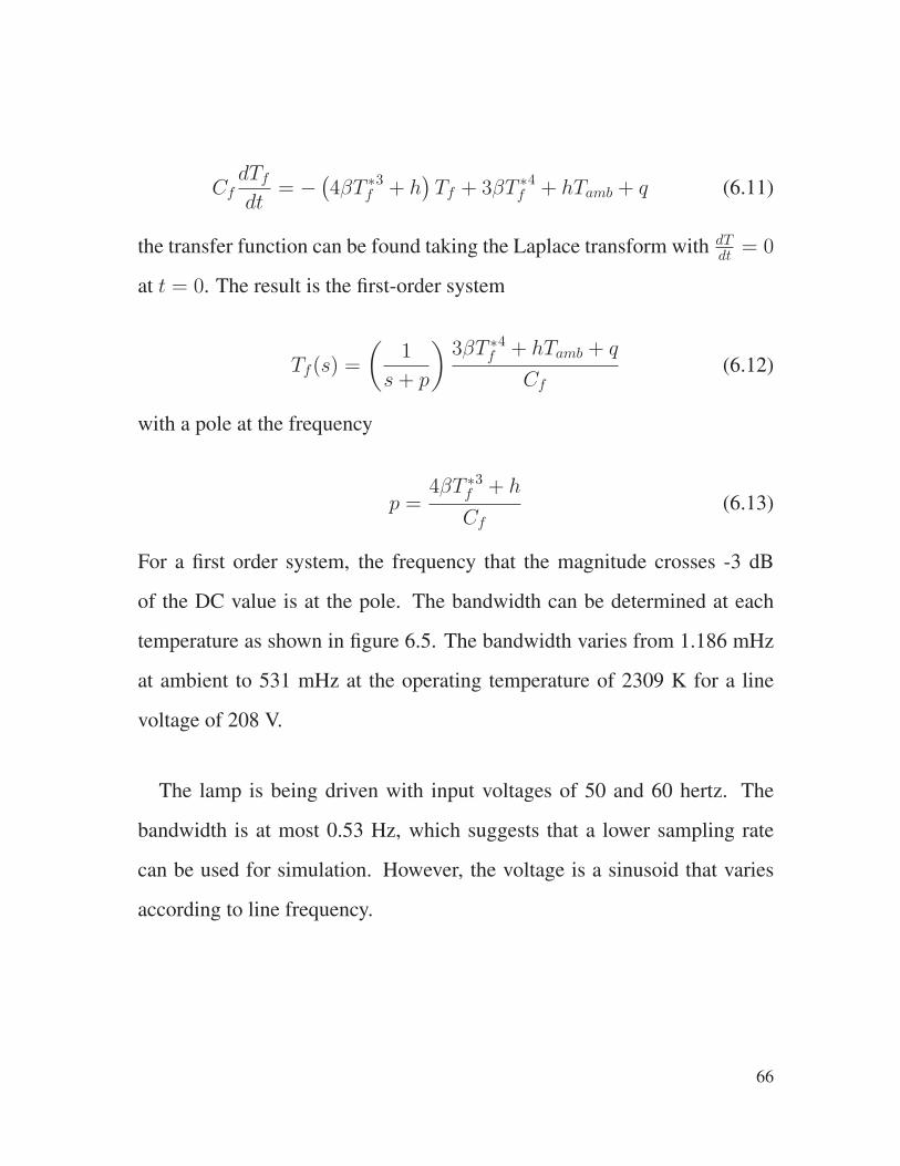
Cf
dTf
dt= −
(
4βT ∗f3 + h
)
Tf + 3βT ∗f4 + hTamb + q (6.11)
the transfer function can be found taking the Laplace transform with dTdt
= 0
at t = 0. The result is the first-order system
Tf(s) =
(
1
s+ p
)
3βT ∗f4 + hTamb + q
Cf
(6.12)
with a pole at the frequency
p =4βT ∗f
3 + h
Cf
(6.13)
For a first order system, the frequency that the magnitude crosses -3 dB
of the DC value is at the pole. The bandwidth can be determined at each
temperature as shown in figure 6.5. The bandwidth varies from 1.186 mHz
at ambient to 531 mHz at the operating temperature of 2309 K for a line
voltage of 208 V.
The lamp is being driven with input voltages of 50 and 60 hertz. The
bandwidth is at most 0.53 Hz, which suggests that a lower sampling rate
can be used for simulation. However, the voltage is a sinusoid that varies
according to line frequency.
66
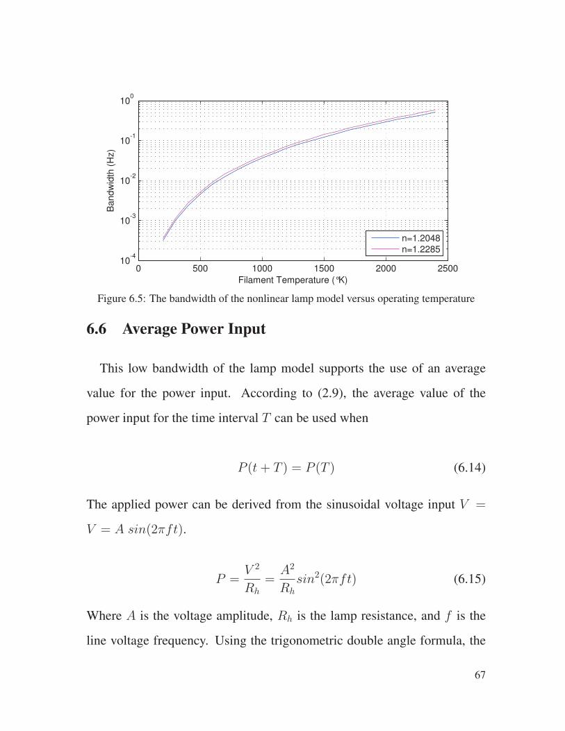
0 500 1000 1500 2000 250010
-4
10-3
10-2
10-1
100
Filament Temperature (°K)
Bandw
idth
(H
z)
n=1.2048
n=1.2285
Figure 6.5: The bandwidth of the nonlinear lamp model versus operating temperature
6.6 Average Power Input
This low bandwidth of the lamp model supports the use of an average
value for the power input. According to (2.9), the average value of the
power input for the time interval T can be used when
P (t+ T ) = P (T ) (6.14)
The applied power can be derived from the sinusoidal voltage input V =
V = A sin(2πft).
P =V 2
Rh
=A2
Rh
sin2(2πft) (6.15)
Where A is the voltage amplitude, Rh is the lamp resistance, and f is the
line voltage frequency. Using the trigonometric double angle formula, the
67

power can be written
P =A2
Rh
[
1
2−
1
2cos(2 · 2πft)
]
(6.16)
If the time interval is chosen to match one half cycle T = 1
2f, then the
average power for the time internal can be found from (2.10)
P = 2f
∫ 1
2f
0
A2
Rh
[
1
2−
1
2cos(2 · 2πfτ)
]
dτ (6.17)
By evaluating the definite integral in (6.17) and rearranging, the average
power can be expressed as
P =A2
2Rh
(6.18)
Which can be further simplified by using the root mean square voltage
P =Vrms
2
Rh
(6.19)
So for finding the average power delivered to the lamp, the time interval
for averaging must be a multiple of the half-cycle period of 1
2f. This is 8.3
milliseconds for 60 Hertz and 10 milliseconds for 50 Hertz.
The effect of powering the lamp with an AC voltage and a DC equivalent
voltage is shown in figure 6.6. In the first case, the input is a 60 Hz sine
wave with an amplitude of 294 volts, the time step is 0.1 milliseconds. The
68

0 0.01 0.02 0.03 0.04 0.05 0.06 0.07
300
400
500
600
700
800
900
1000F
ilam
ent T
em
pera
ture
(°K
)
Time (s)
294 V sine wave, Ts = 0.1 ms
Constant 208V, Ts = 8.3 ms
Constant 208V, Ts = 16.7 ms
Figure 6.6: Lamp startup comparison with AC voltage and constant RMS voltage value
applied
second and third cases were run with a constant voltage of 208 volts, and
a time step 8.3 and 16.7 milliseconds, respectively. The worst case rate of
change of the temperature is when the lamp is cold, which is shown.
With the stress case of the cold start, the average power method showed
good agreement with the 0.1 millisecond simulation model. Even during
the rapid change of temperature during the cold start of the lamp in figure
6.6, the average power method gives an accurate filament temperature. The
error in the temperature after one full voltage cycle is 16.7 milliseconds is
-0.02% for averaging over a half cycle, and -0.63% for averaging over a full
cycle.
69
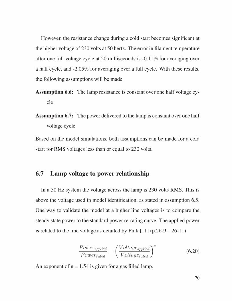
However, the resistance change during a cold start becomes significant at
the higher voltage of 230 volts at 50 hertz. The error in filament temperature
after one full voltage cycle at 20 milliseconds is -0.11% for averaging over
a half cycle, and -2.05% for averaging over a full cycle. With these results,
the following assumptions will be made.
Assumption 6.6: The lamp resistance is constant over one half voltage cy-
cle
Assumption 6.7: The power delivered to the lamp is constant over one half
voltage cycle
Based on the model simulations, both assumptions can be made for a cold
start for RMS voltages less than or equal to 230 volts.
6.7 Lamp voltage to power relationship
In a 50 Hz system the voltage across the lamp is 230 volts RMS. This is
above the voltage used in model identification, as stated in assumption 6.5.
One way to validate the model at a higher line voltages is to compare the
steady state power to the standard power re-rating curve. The applied power
is related to the line voltage as detailed by Fink [11] (p.26-9 – 26-11)
PowerappliedPowerrated
=
(
V oltageappliedV oltagerated
)n
(6.20)
An exponent of n = 1.54 is given for a gas filled lamp.
70
50 100 150 200 250 300 35012
14
16
18
20
22
24
Lamp Voltage (V RMS)
Ste
ady S
tate
Fila
ment R
esis
tance (
Ω)
Single-State Filament Model
Re-rating equation, n=1.54
Figure 6.7: Comparision of lamp filament model prediction of resistance and re-rating
equation. Model fit for the range of 40% to 150% of the rated voltage 208 V, is 99.94 %
The rated power of the heating lamp is 2200 watts at 208 volts RMS, the
single state lamp model was run for line voltages from 180 to 270 volts.
The average steady state resistance of the filament was calculated after the
filament temperature stabilized. The filament resistance from the simulation
agreed rather well with the re-rating equation (6.20), with a fit of R2 =
99.9% for the entire span. The fit is shown in figure 6.7; the predicted
filament resistance from the model at 230 volts was within 0.08% of the
re-rating prediction. This supports using the model at the higher voltage
of 230 volts, as the heat transfer coefficients will give the proper filament
temperature at the higher power levels.
71

Rh
Vs V(t)
230 VAC
50 Hz
Heater
I(t)
Power distribution system Fuser
LSRS
Figure 6.8: Heating lamp circuit with equivalent line resistance and inductance
6.8 Lamp simulation and flicker response
As detailed by Maeda and Takeuchi [21], the line impedances in figure
2.6 can be represented by an equivalent resistor and inductor. From the IEC
specification [3], the phase line reference impedance is 0.24 + j0.15 Ω at
50 Hz, the neutral line reference impedance is 0.16 + j0.1 Ω at 50 Hz. This
gives an equivalent resistance of Rs = 0.4 Ω, and an equivalent inductance
of Ls = 795.8 µH . This circuit is shown in figure 6.8.
As detailed by Maeda andTakeuchi [21], the differential equation that
describes the current in the circuit is
Vs = Ls
dI(t)
dt+RsI(t) +Rh(t)I(t) (6.21)
The line voltage can be determined from the equation
V (t) = Vs(t)−RsI(t)− Ls
dI(t)
dt(6.22)
72

With the lamp filment model derived in the previous section, the startup
of the lamp can be recreated. Using the standard line voltage of 230 volts
RMS at 50 Hz, the instantaneous flicker sensation is calculated using the
simulator by Jourdan [16].
0 0.2 0.4 0.6 0.8 1 1.2 1.4 1.6 1.8 2195
205
215
225
235
Time (s)
Lin
e V
oltage (
V R
MS
)
0 0.2 0.4 0.6 0.8 1 1.2 1.4 1.6 1.8 20
100
200
300
400
Time (s)
Flic
ker
Sensitiv
ity, s
Raw
RMS
Figure 6.9: Simulation of the power line voltage during an unconstrained start of the Nuvera
lamp. The flicker response is calculated using the line voltage, for raw data and RMS
voltage for each half cycle
For on/off control the short-term flicker response Pst is shown for various
levels for on/off switching in table 6.4. Most of the cases, the Pst limit of
1 is violated. The trend is toward higher power and shorter period to keep
the lamp warm, and away from the 8.8 Hz center of the eye-brain flicker
sensitivity.
The simulation of the worst case combination in this table, 100 millisec-
onds and 50% duty cycle, is shown in figure 6.10. The lamp filament does
73

Duty 200 ms 100 ms 50 ms
Cycle period period period
25% 6.74 7.11 2.42
50% 5.54 8.00 2.94
100% 5.35 5.04 1.65
Table 6.4: Short-term flicker (Pst values for on/off switching of the lamp model
2 2.05 2.1 2.15 2.2 2.25224
226
228
230
232
Time (s)
Lin
e V
oltage (
V R
MS
)
2 2.05 2.1 2.15 2.2 2.25118
120
122
124
126
128
Time (s)
Flic
ker
Sensitiv
ity, s
Raw
RMS
Figure 6.10: Line voltage and flicker response for on/off control of the lamp model. Flicker
response calculated using raw voltage and half-cycle RMS values.
not seem to cool off too much from the steady state value and the flicker
sensitivity appears to be driven by the square wave induced by the switch-
ing. The flicker sensitivity is calculated from the raw voltage signal, and the
RMS voltage multiplied by a sine wave. The raw method gives a Pst value
of 8.00, whereas the RMS method gives a Pst of 7.98. This will be needed
later, as the raw voltage data for the 45 kHz switching cannot be evaluated
for significant lengths of time, the RMS voltage will be used instead.
74
6.9 Discussion
As assumption 6.4 states, this model was derived for a cold start of the
lamp with no heating from other sources. In the Nuvera machine, the lamp is
inside a rotating roll. This model lacks the radiative and convective coupling
with the fuser roll core temperature. The lamp surroundings will be heated
from the inside of the core. The filament temperature stabilizes at 2079 K
when full on, where the fuser roll is close to 500 K. Underestimating the
heating from the surroundings may show a longer than actual startup time
for the lamp when the fuser is at temperature.
The ambiguity with the exponent in the tungsten resistance to temperature
relationship (6.1) may create a problem with the later models. The lamp
parameters were able to be fit to both of the exponents, and give the same
accuracy. Without knowing which one is correct, both will be used in the
later analysis.
75

Chapter 7
Power electronics model development
As reviewed in section 2.7, the fuser power controller (FPC) modulates
power to the lamp by varying the duty cycle of a high speed pulse-width
modulated (PWM) signal. The goal of the model developed in this section
is to capture the lamp power applied, for use with the lamp model developed
in chapter 6.
Section 7.1 describes the electrical system and the modeling simplifica-
tions. The combined lamp and power model is detailed in section 7.2. The
method to simulate the electrical system at a tractable sampling interval is
explained in section 7.3. The reduced model shows good agreement with
empirical startup data, replicating the 4.5 second cold start time.
A simulation of the flicker response with the FPC is shown in 7.4.
76
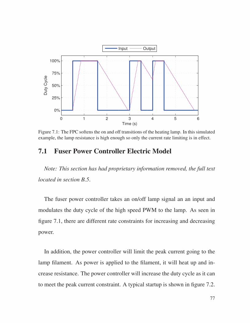
0 1 2 3 4 5 6
0%
25%
50%
75%
100%
Time (s)
Duty
Cycle
Input Output
Figure 7.1: The FPC softens the on and off transitions of the heating lamp. In this simulated
example, the lamp resistance is high enough so only the current rate limiting is in effect.
7.1 Fuser Power Controller Electric Model
Note: This section has had proprietary information removed, the full text
located in section B.5.
The fuser power controller takes an on/off lamp signal an an input and
modulates the duty cycle of the high speed PWM to the lamp. As seen in
figure 7.1, there are different rate constraints for increasing and decreasing
power.
In addition, the power controller will limit the peak current going to the
lamp filament. As power is applied to the filament, it will heat up and in-
crease resistance. The power controller will increase the duty cycle as it can
to meet the peak current constraint. A typical startup is shown in figure 7.2.
77
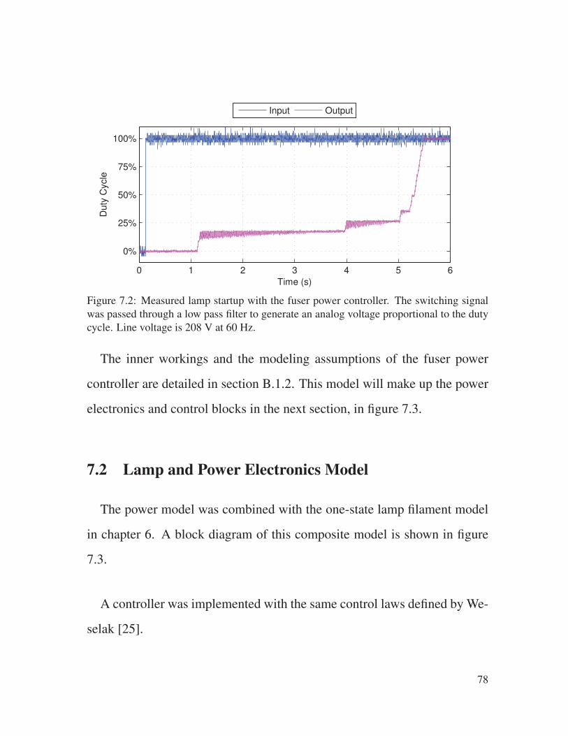
0 1 2 3 4 5 6
0%
25%
50%
75%
100%
Time (s)
Duty
Cycle
Input Output
Figure 7.2: Measured lamp startup with the fuser power controller. The switching signal
was passed through a low pass filter to generate an analog voltage proportional to the duty
cycle. Line voltage is 208 V at 60 Hz.
The inner workings and the modeling assumptions of the fuser power
controller are detailed in section B.1.2. This model will make up the power
electronics and control blocks in the next section, in figure 7.3.
7.2 Lamp and Power Electronics Model
The power model was combined with the one-state lamp filament model
in chapter 6. A block diagram of this composite model is shown in figure
7.3.
A controller was implemented with the same control laws defined by We-
selak [25].
78

control
filament resistance
source voltage
requested duty cycle
lamp power
line voltage
current limiting active
lamp model
power
electronics
on/off signal
Figure 7.3: Block diagram showing interconnectivity between lamp and power controller
subsystems
Information in this section is redacted, full text is located in section B.6
A comparison of the model output for a cold start for 50 and 60 hertz
mains power systems are shown in figure 7.4. The 60 Hz model showed
good agreement with the measured start up time of 4.2 seconds. A variable
dead time was observed where no power is delivered to the lamp, it was
about 1.1 seconds in this measured example.
7.3 Average power and lookup table
The difficulty with combining the fuser and lamp thermal models with
the power electronics is that the time scales are vastly different. Simulating
the full system will take 10,000 times more processing time and storage
79
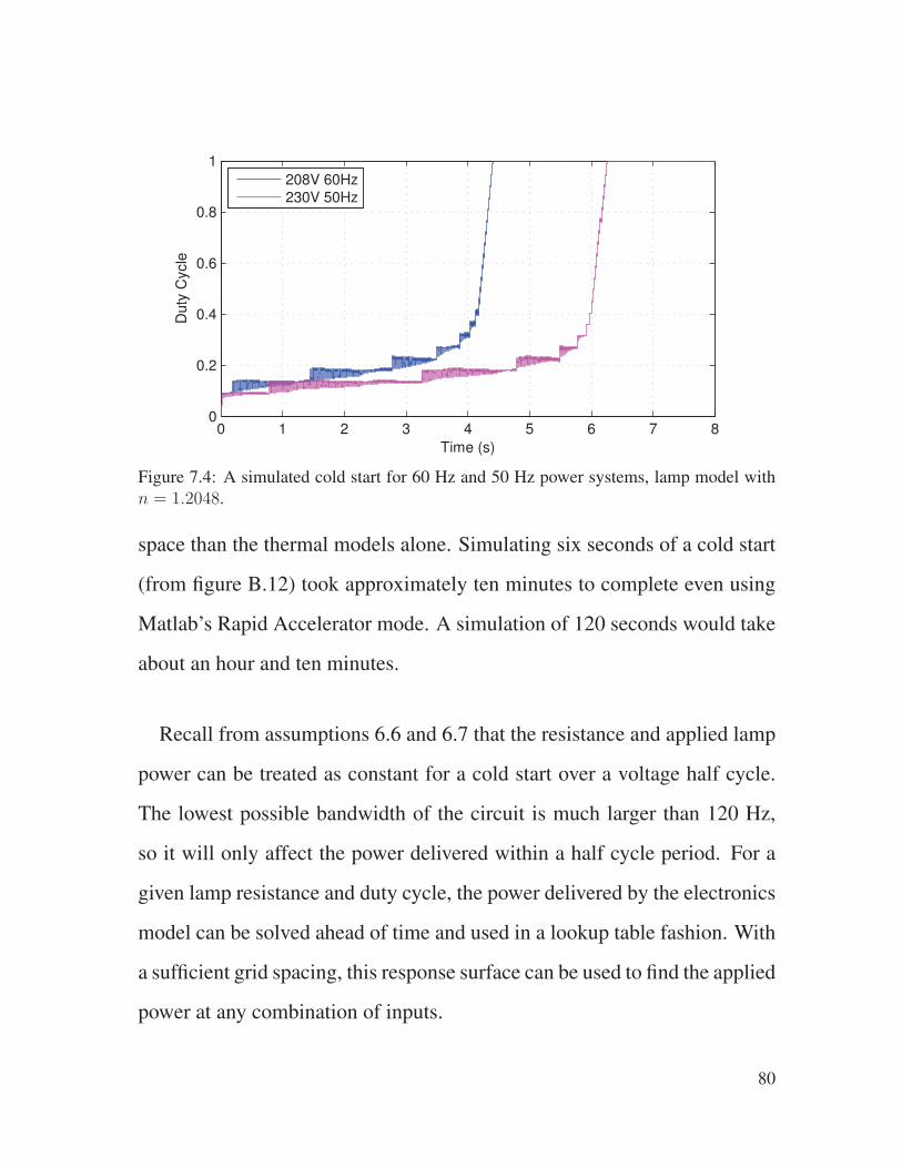
0 1 2 3 4 5 6 7 80
0.2
0.4
0.6
0.8
1
Time (s)
Duty
Cycle
208V 60Hz
230V 50Hz
Figure 7.4: A simulated cold start for 60 Hz and 50 Hz power systems, lamp model with
n = 1.2048.
space than the thermal models alone. Simulating six seconds of a cold start
(from figure B.12) took approximately ten minutes to complete even using
Matlab’s Rapid Accelerator mode. A simulation of 120 seconds would take
about an hour and ten minutes.
Recall from assumptions 6.6 and 6.7 that the resistance and applied lamp
power can be treated as constant for a cold start over a voltage half cycle.
The lowest possible bandwidth of the circuit is much larger than 120 Hz,
so it will only affect the power delivered within a half cycle period. For a
given lamp resistance and duty cycle, the power delivered by the electronics
model can be solved ahead of time and used in a lookup table fashion. With
a sufficient grid spacing, this response surface can be used to find the applied
power at any combination of inputs.
80

This simplification requires knowing when the power system is in lim-
iting mode and not able to increase the duty cycle. The following sets of
lookup tables have to be found
1. Derive a surface for maximum instantaneous current without limiting
in effect to find the isoline at maximum current. This will be the indi-
cator that the FPC is current limiting, and used to signal to the control
not to increment the duty cycle.
2. With current limiting, derive surfaces for the output variables of aver-
age power and RMS line voltage.
To keep the data sets manageable, a set of surfaces was created at a spec-
ified line voltage and lamp inductance. The lookup table was mapped at
each possible duty cycle of the controller. The mesh in the resistance axis
was increased until both models showed agreement, for final mesh spacing
of 0.5 from 1.5 to 22 ohms. A comparison of the cold start sequence for the
100 nanosecond full model and the 16.7 millisecond lookup table model are
shown in figure 7.5. The requested duty cycle of the models is shown, but
the actual value may be lower due to current limiting.
The startup time in figure 7.5 was one full voltage cycle or 16.7 millisec-
onds early over the total 4.5 seconds.
81
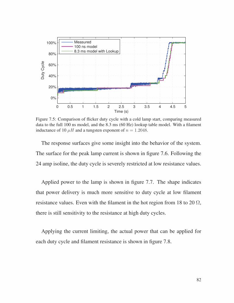
0 0.5 1 1.5 2 2.5 3 3.5 4 4.5 5
0%
20%
40%
60%
80%
100%
Time (s)
Duty
Cycle
Measured
100 ns model
8.3 ms model with Lookup
Figure 7.5: Comparison of flicker duty cycle with a cold lamp start, comparing measured
data to the full 100 ns model, and the 8.3 ms (60 Hz) lookup table model. With a filament
inductance of 10 µH and a tungsten exponent of n = 1.2048.
The response surfaces give some insight into the behavior of the system.
The surface for the peak lamp current is shown in figure 7.6. Following the
24 amp isoline, the duty cycle is severely restricted at low resistance values.
Applied power to the lamp is shown in figure 7.7. The shape indicates
that power delivery is much more sensitive to duty cycle at low filament
resistance values. Even with the filament in the hot region from 18 to 20 Ω,
there is still sensitivity to the resistance at high duty cycles.
Applying the current limiting, the actual power that can be applied for
each duty cycle and filament resistance is shown in figure 7.8.
82
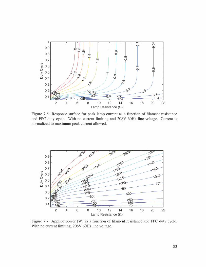
0.30.4 0.4 0.40.5 0.50.5
0.6 0.60.6
0.6
0.6
0.70.7
0.7
0.7
0.7
0.8
0.8
0.8
0.8
0.9
0.9
0.9
0.9
11
1
11.2
1.2
1.2
1.4
1.4
1.4
1.6
1.6
1.6
1.8
1.8
1.8
2
2
2
Lamp Resistance (Ω)
Duty
Cycle
2 4 6 8 10 12 14 16 18 20 22
0.1
0.2
0.3
0.4
0.5
0.6
0.7
0.8
0.9
1
Figure 7.6: Response surface for peak lamp current as a function of filament resistance
and FPC duty cycle. With no current limiting and 208V 60Hz line voltage. Current is
normalized to maximum peak current allowed.
75 75 75150 150 150250
250 250500
500500
750
750750
750
1000
1000
1000
1000
1250
1250
1250
1250
1500
1500
1500
1500
1750
1750
1750
17502000
2000
2000
2000
2500
2500
2500
3000
3000
3000
4000
4000
5000
5000
Lamp Resistance (Ω)
Duty
Cycle
f
2 4 6 8 10 12 14 16 18 20 22
0.1
0.2
0.3
0.4
0.5
0.6
0.7
0.8
0.9
Figure 7.7: Applied power (W) as a function of filament resistance and FPC duty cycle.
With no current limiting, 208V 60Hz line voltage.
83

75 75 75
75150
150 150 150
250250
250 250 250
500
500
500
500 500500
750
750
750
750
750
1000
1000
1000
1000
1250
1250
1250
1250
1500
1500
1500
1500
1750
1750
1750
2000
2000
2000
2500 2500
3000
Lamp Resistance (Ω)
Duty
Cycle
2 4 6 8 10 12 14 16 18 20 22
0.1
0.2
0.3
0.4
0.5
0.6
0.7
0.8
0.9
1
Power
Current Limit
Figure 7.8: Applied power (W) with current limiting as a function of filament resistance
and FPC duty cycle.
7.4 Flicker Response
With the model built in Simulink as described in figure 7.3, the cold start
of the lamp was simulated for 230 volt, 50 hertz power and a filament model
with n = 1.2048 was used.
Recall that in figure 6.9, the line voltage dropped down to 195 volts during
the inrush of the lamp with a ∆VV
= 15%. With the fuser power controller,
the line voltage drop is improved to 224 volts for a ∆VV
= 2.6%. The peak
flicker sensation in figure 6.9 was about 300 to 325, now reduced to 19. The
lamp took approximately 5.5 seconds to start up at this higher voltage of
230 V.
84
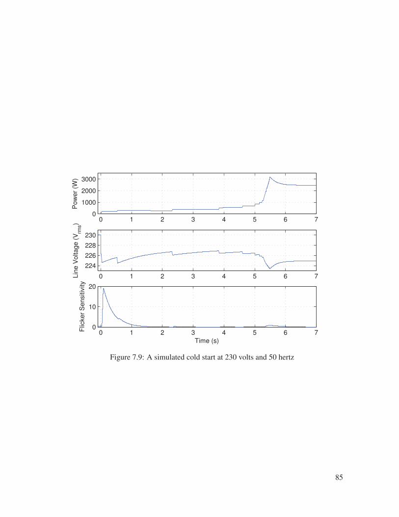
0 1 2 3 4 5 6 70
1000
2000
3000
Pow
er
(W)
0 1 2 3 4 5 6 7
224
226
228
230
Lin
e V
oltage (
Vrm
s)
0 1 2 3 4 5 6 70
10
20
Flic
ker
Sensitiv
ity
Time (s)
Figure 7.9: A simulated cold start at 230 volts and 50 hertz
85

7.5 Discussion
One consequence of the response surfaces found in section 7.3, is that the
applied power to the lamp filament is dependent on both the FPC duty cycle
and the lamp filament resistance. If the power level is changed drastically,
there will be a transient in the applied power until the filament resistance sta-
bilizes to the new power level. Precise control of the power is difficult using
an open loop duty cycle. By design, the FPC measures the lamp voltage and
current, which will allow calculation of the instantaneous power.
86
Chapter 8
Combined thermal and electrical model
Now that the power controller and the lamp filament components have
been identified, the complete system block diagram is described in sec-
tion 8.1.
The current controls and their behavior are explained and demonstrated
in section 8.2. Data from a Nuvera machine with a fuser power controller
is used to show the limit cycles present in the current system and justify
approximating the temperature controller with an on/off relay.
The known variable temperature droop response is explored with the
model in section 8.3. The startup time of the lamp versus based on the time
the lamp is off is evaluated. The model shows agreement with the behavior,
but all of the characteristics of the system are not captured.
87

lamp
power
on/off
signal
power
control
fuser
model
Fuser surface temp
temperature
control
sensor
R
error
-
+
Mode
Figure 8.1: Block diagram for complete thermo-electric system. The reference R and the
Mode are provided by the supervisory control.
An alternate feedback compensator is explored in section 8.4, and the
presence of limit cycles in the system is found to be an outcome of the
design.
8.1 Model Block Diagram
The block diagram of the system model is shown in figure 8.1.
Power Control Block The system from figure 7.3, containing the subcom-
ponents:
• Electrical circuit
• Lamp filament thermo-electric model
• Power controller
The output is the power applied to the fuser thermal system. With
88

assumption 3.2, 100% of the the electrical power is applied to the fuser
as heat.
Fuser Thermal Model The model developed in chapter 5, containing a
sliding factor to allow adjustment of the thermal load of the fused me-
dia.
Sensor The dynamics can be represented by a first order system with a fixed
time constant, as in assumption 3.2.
Temperature Control The controller will be explored in the next section.
Supervisory Control Not shown. The higher level machine control changes
the temperature set point and schedules print jobs. This affects the tim-
ing of the dynamic mode transitions of the fuser thermal system. A few
important notes are also highlighted in the next section.
8.2 Current Controls and Behavior
Note: This section has had proprietary information removed, the full text
located in section B.8
To facilitate the analysis of the control performance, the temperature con-
trol error can be normalized using the equation:
e =x2 − r2emax
(8.1)
89
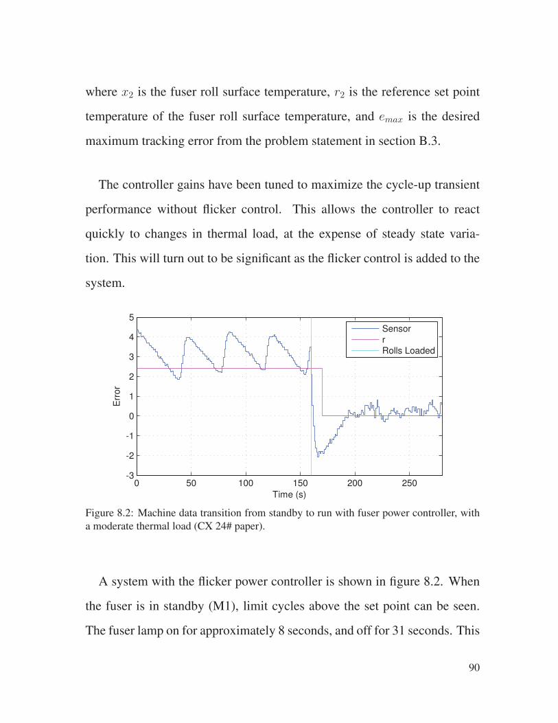
where x2 is the fuser roll surface temperature, r2 is the reference set point
temperature of the fuser roll surface temperature, and emax is the desired
maximum tracking error from the problem statement in section B.3.
The controller gains have been tuned to maximize the cycle-up transient
performance without flicker control. This allows the controller to react
quickly to changes in thermal load, at the expense of steady state varia-
tion. This will turn out to be significant as the flicker control is added to the
system.
0 50 100 150 200 250-3
-2
-1
0
1
2
3
4
5
Time (s)
Err
or
Sensor
r
Rolls Loaded
Figure 8.2: Machine data transition from standby to run with fuser power controller, with
a moderate thermal load (CX 24# paper).
A system with the flicker power controller is shown in figure 8.2. When
the fuser is in standby (M1), limit cycles above the set point can be seen.
The fuser lamp on for approximately 8 seconds, and off for 31 seconds. This
90
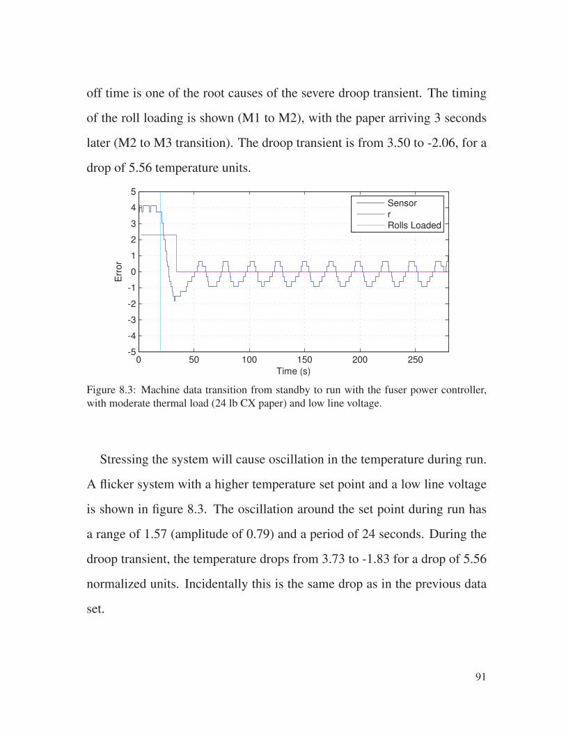
off time is one of the root causes of the severe droop transient. The timing
of the roll loading is shown (M1 to M2), with the paper arriving 3 seconds
later (M2 to M3 transition). The droop transient is from 3.50 to -2.06, for a
drop of 5.56 temperature units.
0 50 100 150 200 250-5
-4
-3
-2
-1
0
1
2
3
4
5
Time (s)
Err
or
Sensor
r
Rolls Loaded
Figure 8.3: Machine data transition from standby to run with the fuser power controller,
with moderate thermal load (24 lb CX paper) and low line voltage.
Stressing the system will cause oscillation in the temperature during run.
A flicker system with a higher temperature set point and a low line voltage
is shown in figure 8.3. The oscillation around the set point during run has
a range of 1.57 (amplitude of 0.79) and a period of 24 seconds. During the
droop transient, the temperature drops from 3.73 to -1.83 for a drop of 5.56
normalized units. Incidentally this is the same drop as in the previous data
set.
91
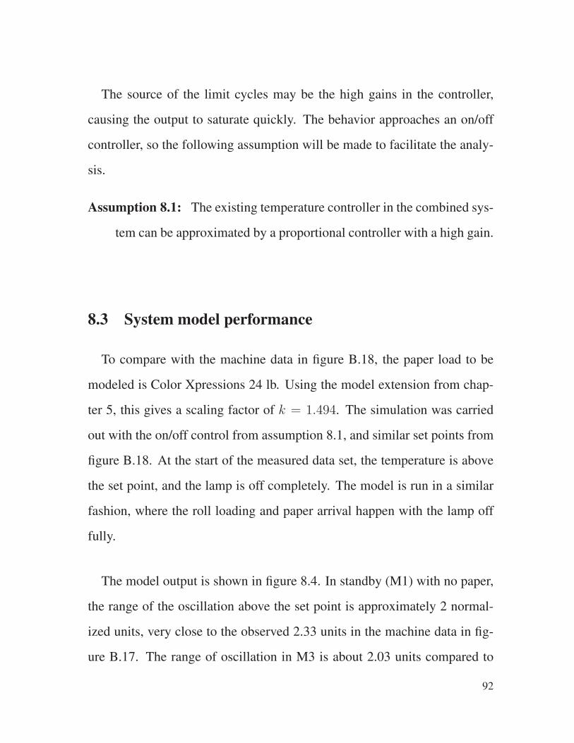
The source of the limit cycles may be the high gains in the controller,
causing the output to saturate quickly. The behavior approaches an on/off
controller, so the following assumption will be made to facilitate the analy-
sis.
Assumption 8.1: The existing temperature controller in the combined sys-
tem can be approximated by a proportional controller with a high gain.
8.3 System model performance
To compare with the machine data in figure B.18, the paper load to be
modeled is Color Xpressions 24 lb. Using the model extension from chap-
ter 5, this gives a scaling factor of k = 1.494. The simulation was carried
out with the on/off control from assumption 8.1, and similar set points from
figure B.18. At the start of the measured data set, the temperature is above
the set point, and the lamp is off completely. The model is run in a similar
fashion, where the roll loading and paper arrival happen with the lamp off
fully.
The model output is shown in figure 8.4. In standby (M1) with no paper,
the range of the oscillation above the set point is approximately 2 normal-
ized units, very close to the observed 2.33 units in the machine data in fig-
ure B.17. The range of oscillation in M3 is about 2.03 units compared to
92
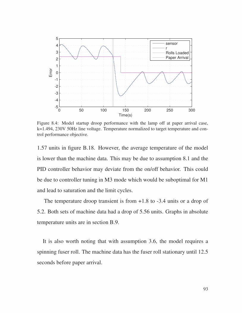
0 50 100 150 200 250 300-5
-4
-3
-2
-1
0
1
2
3
4
5
Time(s)
Err
or
sensorr
Rolls LoadedPaper Arrival
Figure 8.4: Model startup droop performance with the lamp off at paper arrival case,
k=1.494, 230V 50Hz line voltage. Temperature normalized to target temperature and con-
trol performance objective.
1.57 units in figure B.18. However, the average temperature of the model
is lower than the machine data. This may be due to assumption 8.1 and the
PID controller behavior may deviate from the on/off behavior. This could
be due to controller tuning in M3 mode which would be suboptimal for M1
and lead to saturation and the limit cycles.
The temperature droop transient is from +1.8 to -3.4 units or a drop of
5.2. Both sets of machine data had a drop of 5.56 units. Graphs in absolute
temperature units are in section B.9.
It is also worth noting that with assumption 3.6, the model requires a
spinning fuser roll. The machine data has the fuser roll stationary until 12.5
seconds before paper arrival.
93
0 50 100 150 200 250 3000
500
1000
1500
2000
2500
3000
3500
Time (s)
Pow
er
(W)
qin
q12
Figure 8.5: Model input power and heat flow for the lamp off at paper arrival case, k=1.494,
230V 50Hz line voltage. Cycle-up transient portion of the simulation shown.
To help facilitate the analysis, the heat flow q12 between the layers of the
fuser rollm1 andm2 can be calculated. The heat flow will give an indication
of how much heat being applied to the core makes it to the paper.
q12(t) = h1 (x1(t)− x2(t)) (8.2)
The result from the lamp off at the paper arrival case is shown in fig-
ure 8.5. The on/off command to the fuser power controller is shown on the
power axis, with P = 2600W corresponding to the on condition and P = 0
for the off condition. The lamp input power is q and the heat flow between
layersm1 andm2 is q12.
94

0 50 100 150 200 250 300
5
10
15
20
Time (s)
Fila
ment R
esis
tance (
Ω)
Figure 8.6: Model filament resistance for the lamp off at paper arrival case, k=1.494, 230V
50 Hz line voltage
The lamp is commanded to turn on at t = 123.8 s. The fuser power
controller reaches full lamp power 4.2 seconds later. The heat flow reaches
95% of the final value 14.8 seconds after the lamp reaches full power. Once
the heat flow reaches this value, the fuser roll surface temperature (x2) can
increase at its maximum rate. This helps subdivide the temperature droop,
one-fourth of the delay is due to the flicker constraints in the electrical sys-
tem, and three-fourths is due to the thermal response of the fuser.
The filament resistance is shown in figure 8.6. At steady state, the fila-
ment resistance is 20.4 Ω with a temperature of 2,479 K. With the on/off
switching in M1 (t < 150 s), the lamp is off for about 50 seconds. Starting
from a resistance of 3.3 Ω or 550 K, it takes 5.3 seconds for the lamp to re-
turn to full power. The amount of time the lamp is off decreases after paper
95
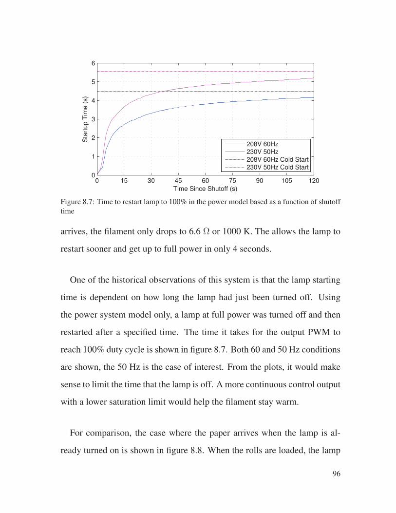
0 15 30 45 60 75 90 105 1200
1
2
3
4
5
6
Time Since Shutoff (s)
Sta
rtup T
ime (
s)
208V 60Hz230V 50Hz
208V 60Hz Cold Start230V 50Hz Cold Start
Figure 8.7: Time to restart lamp to 100% in the power model based as a function of shutoff
time
arrives, the filament only drops to 6.6 Ω or 1000 K. The allows the lamp to
restart sooner and get up to full power in only 4 seconds.
One of the historical observations of this system is that the lamp starting
time is dependent on how long the lamp had just been turned off. Using
the power system model only, a lamp at full power was turned off and then
restarted after a specified time. The time it takes for the output PWM to
reach 100% duty cycle is shown in figure 8.7. Both 60 and 50 Hz conditions
are shown, the 50 Hz is the case of interest. From the plots, it would make
sense to limit the time that the lamp is off. A more continuous control output
with a lower saturation limit would help the filament stay warm.
For comparison, the case where the paper arrives when the lamp is al-
ready turned on is shown in figure 8.8. When the rolls are loaded, the lamp
96
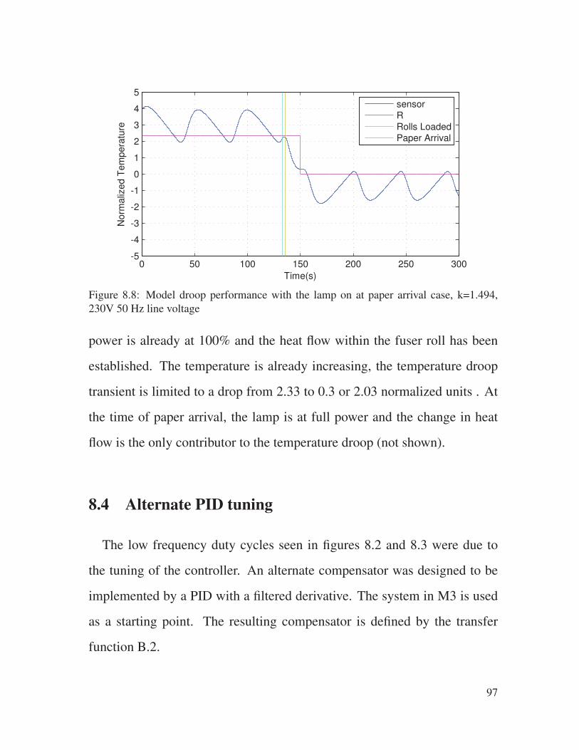
0 50 100 150 200 250 300-5
-4
-3
-2
-1
0
1
2
3
4
5
Time(s)
Norm
aliz
ed T
em
pera
ture
sensorR
Rolls LoadedPaper Arrival
Figure 8.8: Model droop performance with the lamp on at paper arrival case, k=1.494,
230V 50 Hz line voltage
power is already at 100% and the heat flow within the fuser roll has been
established. The temperature is already increasing, the temperature droop
transient is limited to a drop from 2.33 to 0.3 or 2.03 normalized units . At
the time of paper arrival, the lamp is at full power and the change in heat
flow is the only contributor to the temperature droop (not shown).
8.4 Alternate PID tuning
The low frequency duty cycles seen in figures 8.2 and 8.3 were due to
the tuning of the controller. An alternate compensator was designed to be
implemented by a PID with a filtered derivative. The system in M3 is used
as a starting point. The resulting compensator is defined by the transfer
function B.2.
97

0 50 100 150 200 250 300-5
-4
-3
-2
-1
0
1
2
3
4
5
Time(s)
Err
or
sensorr
Rolls LoadedPaper Arrival
Figure 8.9: Combined model droop performance with alternate PID gain factors, with
k=1.494, and 230V 50 Hz line voltage.
The resulting performance is shown in figure 8.9. There is still cycle-up
droop is still present as the system has to change power levels from 350
watts to 2100 watts. There is a very small periodic variation in the temper-
ature variation.
As seen in figure 8.10, the control input still takes on on/off switching
behavior. With a higher bandwidth controller, the switching rate is faster
and the thermal system acts like a low pass filter. Also, the limit cycles in
the input seem to be in response to the derivative of the output rather than
the error.
98

0 50 100 150 200 250 3000
500
1000
1500
2000
2500
3000
3500
Time (s)
Pow
er
(W)
qin
q12
Figure 8.10: Lamp input for combined model with alternate PID gain factors, with k=1.494,
and 230V 50 Hz line voltage.
8.5 Discussion
Combining the individual system models allowed some replication of the
temperature droop phenomenon. However, recall from figure 3.9 that a fast
transient in the thermal system that was not captured. This may explain the
difficulties replicating the machine data faithfully. The simplification of the
controller according to assumption 8.1 may have increased the severity of
the limit cycles in the model.
Additional limitations of the existing controller are detailed in section
B.9.
Assumption 6.4 has the ambient temperature in the lamp model as room
temperature, 22 C. In reality, it is subject to the temperature inside the
99

fuser roll core. This discrepancy will make the startup time of the model
marginally worse than the real system.
From the timing data in section 8.3, the total cycle-up droop time of 19
seconds can be subdivided into two parts:
1. Delay to bring the lamp to full power on due to constraints in the fuser
power controller (4.2 seconds, 22%)
2. Delay of of the system to change from standby to run power levels
(14.8 seconds, 78%)
Both of these portions will be addressed in the next section.
100
Chapter 9
Open-loop optimal control problem
In this chapter, the open-loop optimal control is formulated and solved to
gain insight into potential control strategies. The power limiting behavior
of the fuser power controller was found to be extremely non-linear. Even
the relationship between FPC duty cycle and applied power is dependent
on time-varying resistance of the filament. It would be difficult if not im-
possible to incorporate the FPC constraints into the problem. A system
architecture is defined in section 9.1 so that the boundary value problem can
be made tractable.
The basic problem is formulated as a regulator problem, where the fuser
roll surface temperature is kept constant while the system is subjected to
thermal load disturbances. The cost functional is derived in section 9.2, and
the optimal control boundary value problem is formulated in section 9.3.
101
The nominal timing or a typical cycle-up sequence (the flight plan) is
detailed in section 9.4. The solution of the boundary value problem for this
flight plan is shown in section 9.5.
In section 9.6, the optimal input trajectory is used with the power response
surfaces from section 7.3 to back calculate the needed duty cycle. The rate
of change of the duty cycle is measured, and can be compared to the con-
straints in the FPC. In the cost functional, the balance between the control
effort and the tracking error can be adjusted to meet the FPC constraints.
A second order analysis in section 9.7 examines the effect of varying load
timing and initial pressure roll temperature. This gives additional insight
and may lead to system improvements in the cycle-up behavior.
9.1 Integrated Control
One of the difficulties with controlling a system with the fuser power
controller is the delay introduced by the system interconnections. Looking
at the controller to power control blocks from figure 8.1, the on/off pattern
from the temperature control is ultimately driving the high speed PWM.
As seen in figure B.21, the temperature control output communicates the de-
sired lamp power level by the number of on pulses in the pulse train. A more
102

PWM
control
Lamp
Power
electronics
Low speed
On/off pulses
Power Control
fuser
temperature
control
error
High
speed
duty cycle
lamp
resistancelamp
power
lamp
current
On/off
Figure 9.1: The multiple timing rates of the temperature control and power control systems
pose a problem for control. The on/off signal in green is ultimately driving the duty cycle
of the high speed PWM in red.
efficient way to drive the power controller would be to communicate the re-
quested power directly, or integrate the temperature and power controllers
into one system. For this analysis, the following will be assumed:
Assumption 9.1: The temperature controller can directly control the duty
cycle of the high speed PWM in the fuser power controller
If the optimal control problem can be solved in terms of power input to the
thermal system, the power system model can be used to determine if the
input trajectory meets the fuser power controller constraints.
9.2 Cost Functional
Recall that the state equations from (5.3) are
103

x =
A1x+Bu+W1d for M1
A2x+Bu+W1d for M2
A3x+Bu+W2d for M3
(9.1)
The objective is to track a given reference value r with the states x with
minimal control effort u. A quadratic cost functional can be used:
J =1
2
∫ tf
t0
(
(x− r)TQ(x− r) + uTRu)
dt (9.2)
Q is a diagonal matrix with the relative weighting of the error of each
state x to a reference r.
Q =
0 0 0 0
0 1 0 0
0 0 0 0
0 0 0 0
emax2
(9.3)
r =
0
r2
0
0
(9.4)
104
Where the reference is the desired fuser roll surface temperature. The
divisor, emax is the maximum desired error of the surface temperature to the
reference. In this case, the control performance objective is used.
The input can be weighted by the maximum lamp input. This penalizes
using full power of the lamp as much as being off by the performance ob-
jective.
R =1
umax2
(9.5)
To make the relationship between the weighting of the tracking error and
the control effort more clear, the cost function can be reduced to a scalar
case:
J =1
2
∫ tf
t0
(
(
x2 − r2emax
)2
+
(
u
umax
)2)
dt (9.6)
9.3 Optimal control boundary value problem
The optimal control problem becomes: For t ∈ [t0, tf ], minimize the cost
functional
J =1
2
∫ tf
t0
(x− r)TQ(x− r) + uTRudt (9.7)
105
Subject to
x =
A1x+Bu+W1d for t ∈ [t0, t1)
A2x+Bu+W1d for t ∈ [t1, t2)
A3x+Bu+W2d for t ∈ [t2, tf ]
(9.8)
u ∈ [0, umax] (9.9)
The Hamiltonian can be formed from (2.14), using the cost functional
(9.7) and the state equation (9.1)
H =1
2
[
(x− r)TQ(x− r) + uTRu]
+ pT [Aix+Bu+Wjd] (9.10)
The state equation is given by the partial derivative of (9.10) with respect
to the costate, as in (2.15)
x =∂H
∂p= Aix+Bu+Wjd (9.11)
The costate equation is given by the partial derivative of (9.10) with re-
spect to the state, as in (2.16).
p = −∂H
∂x= −
[
Q (x− r) + AjTp]
(9.12)
106
The stationary condition is the partial derivative with respect to the input,
as in (2.17).
0 =∂H
∂u= Ru+BTp (9.13)
The input can be solved for
u = −R−1BTp (9.14)
Pontryagin’s minimum principle (2.20) can be applied to (9.14) and (9.9)
u =
0 for −R−1BTp ≤ 0
−R−1BTp for 0 < −R−1BTp < umax
umax for −R−1BTp ≥ umax
(9.15)
The initial conditions are applied to the state variables as in (2.18)
x(t0) = x0 (9.16)
The final conditions are applied to the costate variables. The final state
will be free in this problem, so there is no weight on the final state: h = 0.
The boundary condition in (2.19) simplifies to
p(tf) = 0 (9.17)
107
which in this four state problem becomes
p(tf) =
0
0
0
0
(9.18)
9.4 Flight plan
As a starting point, a typical cycle up sequence will be used to find the
optimal input and state trajectories. The machine will start in an idle state
with the fuser roll temperature stabilized. The rolls will be loaded three
seconds before the paper arrives, the print job will last through the end of
the time interval. The constraints and starting conditions are summarized in
table 9.1. Actual temperature set point values are shown in table B.7. To
simplify the problem, the pressure roll temperatures will start at ambient.
The maximum lamp power umax is the power delivered by the lamp at
100% duty cycle. This can be calculated at a given line voltage, but the line
voltage will drop with the current draw of the lamp. This can be calculated
from the lamp filament model from figure 6.8. For a source voltage of 230
volts, the power stabilizes at 2475 watts with a line voltage of 224.8 volts.
108
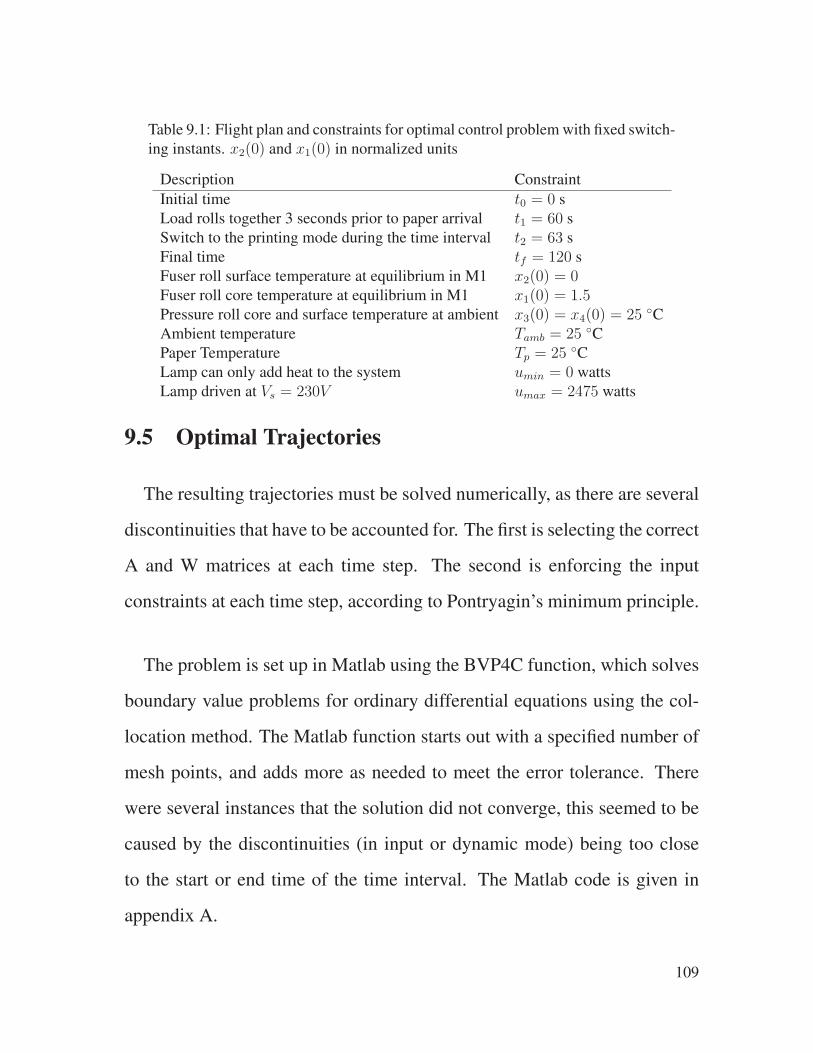
Table 9.1: Flight plan and constraints for optimal control problemwith fixed switch-
ing instants. x2(0) and x1(0) in normalized units
Description Constraint
Initial time t0 = 0 sLoad rolls together 3 seconds prior to paper arrival t1 = 60 sSwitch to the printing mode during the time interval t2 = 63 sFinal time tf = 120 sFuser roll surface temperature at equilibrium in M1 x2(0) = 0Fuser roll core temperature at equilibrium in M1 x1(0) = 1.5Pressure roll core and surface temperature at ambient x3(0) = x4(0) = 25 CAmbient temperature Tamb = 25 CPaper Temperature Tp = 25 CLamp can only add heat to the system umin = 0 wattsLamp driven at Vs = 230V umax = 2475 watts
9.5 Optimal Trajectories
The resulting trajectories must be solved numerically, as there are several
discontinuities that have to be accounted for. The first is selecting the correct
A and W matrices at each time step. The second is enforcing the input
constraints at each time step, according to Pontryagin’s minimum principle.
The problem is set up in Matlab using the BVP4C function, which solves
boundary value problems for ordinary differential equations using the col-
location method. The Matlab function starts out with a specified number of
mesh points, and adds more as needed to meet the error tolerance. There
were several instances that the solution did not converge, this seemed to be
caused by the discontinuities (in input or dynamic mode) being too close
to the start or end time of the time interval. The Matlab code is given in
appendix A.
109
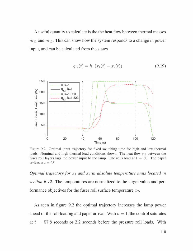
A useful quantity to calculate is the the heat flow between thermal masses
m11 andm12. This can show how the system responds to a change in power
input, and can be calculated from the states
q12(t) = h1 (x1(t)− x2(t)) (9.19)
0 20 40 60 80 100 1200
500
1000
1500
2000
2500
Time (s)
Lam
p P
ow
er,
Heat F
low
(W
)
u, k=1
q12
, k=1
u, k=1.823q
12, k=1.823
Figure 9.2: Optimal input trajectory for fixed switching time for high and low thermal
loads. Nominal and high thermal load conditions shown. The heat flow q12 between thefuser roll layers lags the power input to the lamp. The rolls load at t = 60. The paperarrives at t = 63
Optimal trajectory for x1 and x2 in absolute temperature units located in
section B.12. The temperatures are normalized to the target value and per-
formance objectives for the fuser roll surface temperature x2.
As seen in figure 9.2 the optimal trajectory increases the lamp power
ahead of the roll loading and paper arrival. With k = 1, the control saturates
at t = 57.8 seconds or 2.2 seconds before the pressure roll loads. With
110

0 20 40 60 80 100 120-2
-1
0
1
2
3
4
5
6
7
8
9
10
Time (s)
Norm
aliz
ed T
em
pera
ture
x1, k=1
x2, k=1
x1, k=1.823
x2, k=1.823
Figure 9.3: Optimal state trajectory for fuser roll states x1 and x2. The error is minimized
between the fuser roll surface temperature x2 and a reference of 0.
0 20 40 60 80 100 12025
30
35
40
45
50
Time (s)
Tem
pera
ture
(°C
)
x3, k=1
x4, k=1
x3, k=1.823
x4, k=1.823
Figure 9.4: Optimal state trajectory for pressure roll states x3 and x4 for the fixed switching
time problem
k = 1.823, the control saturates at t = 52.7 seconds or 7.3 seconds before
loading the pressure roll.
111
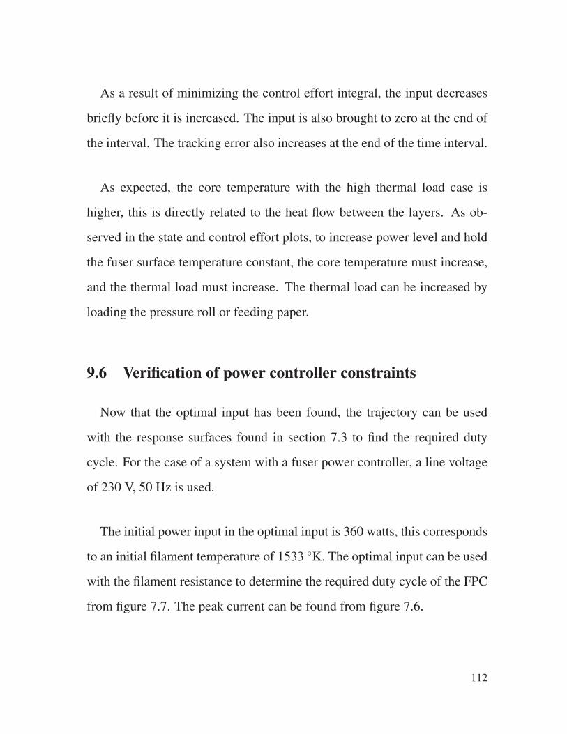
As a result of minimizing the control effort integral, the input decreases
briefly before it is increased. The input is also brought to zero at the end of
the interval. The tracking error also increases at the end of the time interval.
As expected, the core temperature with the high thermal load case is
higher, this is directly related to the heat flow between the layers. As ob-
served in the state and control effort plots, to increase power level and hold
the fuser surface temperature constant, the core temperature must increase,
and the thermal load must increase. The thermal load can be increased by
loading the pressure roll or feeding paper.
9.6 Verification of power controller constraints
Now that the optimal input has been found, the trajectory can be used
with the response surfaces found in section 7.3 to find the required duty
cycle. For the case of a system with a fuser power controller, a line voltage
of 230 V, 50 Hz is used.
The initial power input in the optimal input is 360 watts, this corresponds
to an initial filament temperature of 1533 K. The optimal input can be used
with the filament resistance to determine the required duty cycle of the FPC
from figure 7.7. The peak current can be found from figure 7.6.
112

0 20 40 60 80 100 1200
1000
2000
3000Lamp Input
Lam
pP
ow
er
(W)
0 20 40 60 80 100 1200
0.5
1
Norm
aliz
ed C
urr
ent
Peak Lamp Current
0 20 40 60 80 100 120-0.2
0
0.2Time Rate of Change of Duty Cycle
Norm
aliz
ed R
ate
0 20 40 60 80 100 1200
0.5
1
Duty
Cycle
Figure 9.5: Optimal input trajectory from figure 9.2, with power system time response for
thermal load k=1.823 and 230V 50Hz Line voltage. Duty cycle is shown with 100% equal
to 2475 watts for comparison. Peak current and duty cycle rate of change normalized by
constraints defined in section B.6
113
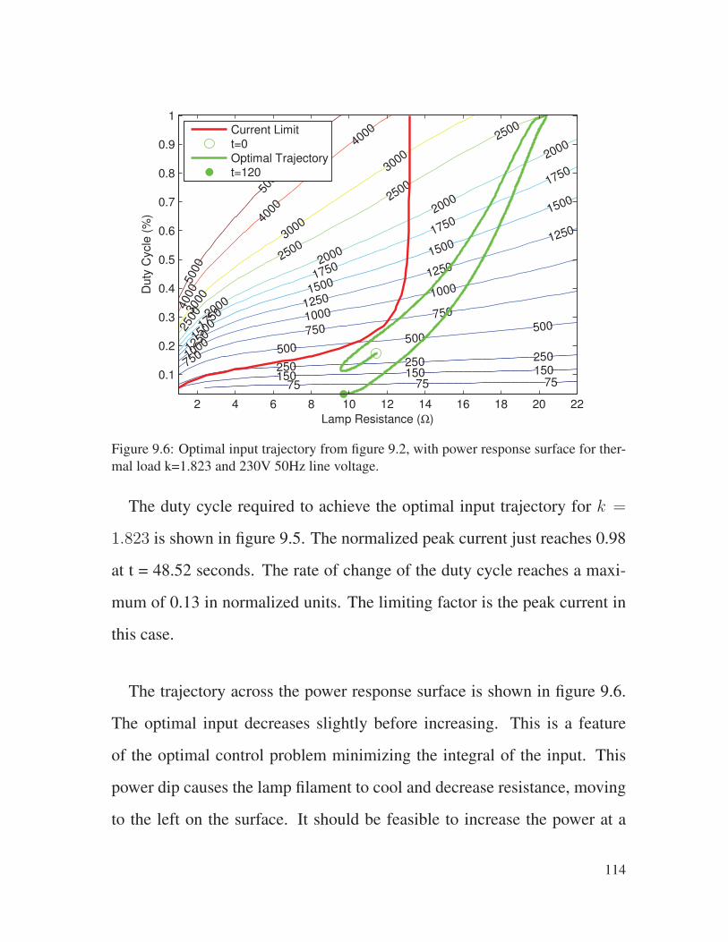
75 75 75150 150 150250 250 250500
500500
750
750
750
1000
1000
1000
1250
1250
1250
1250
1500
1500
1500
1500
1750
1750
1750
1750
2000
2000
2000
20002500
2500
2500
2500
3000
3000
3000
4000
4000
4000
5000
5000
Duty
Cycle
(%
)
Lamp Resistance (Ω)
2 4 6 8 10 12 14 16 18 20 22
0.1
0.2
0.3
0.4
0.5
0.6
0.7
0.8
0.9
1Current Limitt=0
Optimal Trajectoryt=120
Figure 9.6: Optimal input trajectory from figure 9.2, with power response surface for ther-
mal load k=1.823 and 230V 50Hz line voltage.
The duty cycle required to achieve the optimal input trajectory for k =
1.823 is shown in figure 9.5. The normalized peak current just reaches 0.98
at t = 48.52 seconds. The rate of change of the duty cycle reaches a maxi-
mum of 0.13 in normalized units. The limiting factor is the peak current in
this case.
The trajectory across the power response surface is shown in figure 9.6.
The optimal input decreases slightly before increasing. This is a feature
of the optimal control problem minimizing the integral of the input. This
power dip causes the lamp filament to cool and decrease resistance, moving
to the left on the surface. It should be feasible to increase the power at a
114
faster rate if the power does not dip first.
9.7 Second order optimization
In reality, the pressure roll temperature is not measured or controlled,
so its temperature is an outcome of the run sequence. As a second order
analysis, the pressure roll loading time will be varied along with the initial
pressure roll temperatures. For simplicity, the temperature of the pressure
roll is assumed to be stabilized, x3 = x4.
Inital Pressure Roll Temperature (°C)
Loadin
g tim
ing b
efo
re job (
s)
40 60 80 100 1200
5
10
15
20
25
30
13
14
15
16
17
18
Figure 9.7: Cost functional vs loading time and initial pressure roll temperature for k=1.
Gaps in the plot are due to convergence errors with the numerical solver. The minimum is
at (121, 8)
The optimal control BVP was solved for each case of a 13 × 16 mesh
for pressure roll temperature and loading time before the print job. The cost
function was calculated at each mesh point. As shown in figure 9.7, the
115
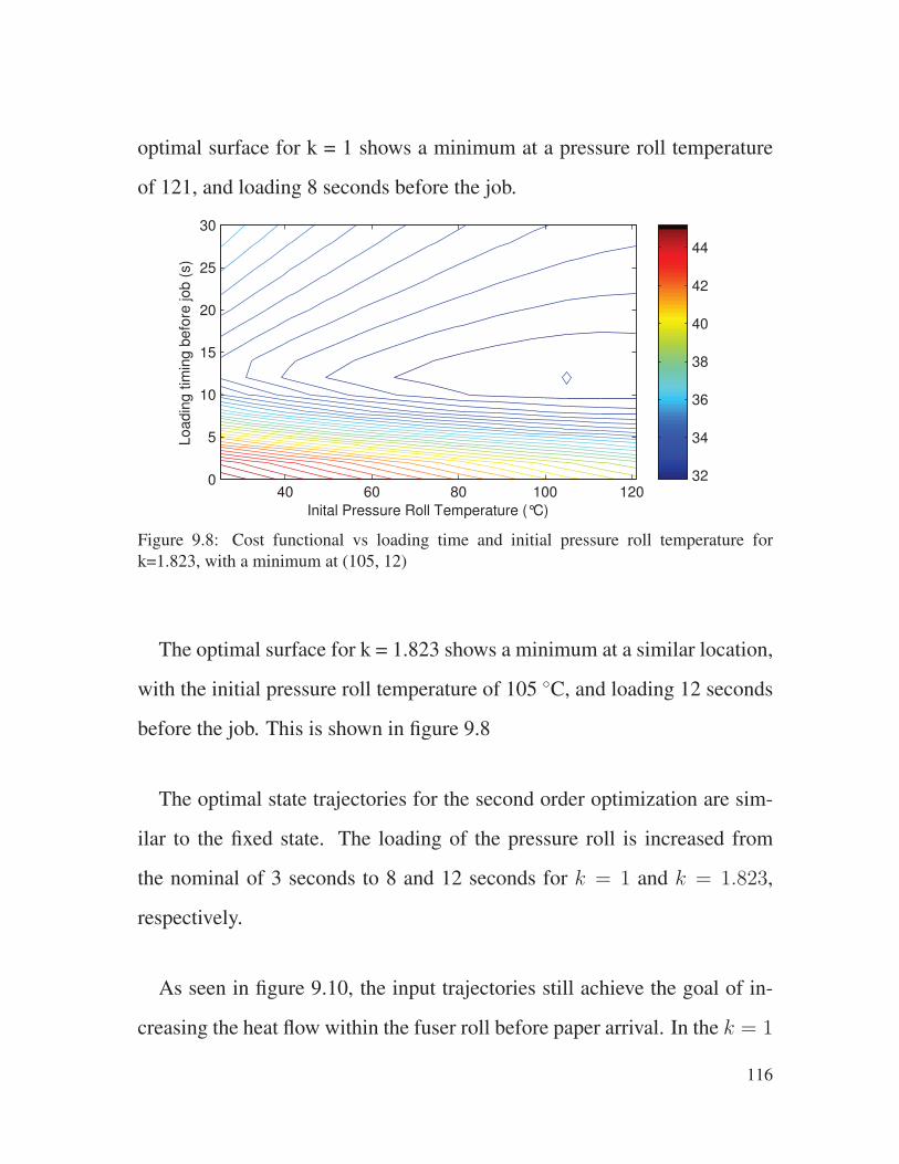
optimal surface for k = 1 shows a minimum at a pressure roll temperature
of 121, and loading 8 seconds before the job.
Inital Pressure Roll Temperature (°C)
Loadin
g tim
ing b
efo
re job (
s)
40 60 80 100 1200
5
10
15
20
25
30
32
34
36
38
40
42
44
Figure 9.8: Cost functional vs loading time and initial pressure roll temperature for
k=1.823, with a minimum at (105, 12)
The optimal surface for k = 1.823 shows a minimum at a similar location,
with the initial pressure roll temperature of 105 C, and loading 12 seconds
before the job. This is shown in figure 9.8
The optimal state trajectories for the second order optimization are sim-
ilar to the fixed state. The loading of the pressure roll is increased from
the nominal of 3 seconds to 8 and 12 seconds for k = 1 and k = 1.823,
respectively.
As seen in figure 9.10, the input trajectories still achieve the goal of in-
creasing the heat flow within the fuser roll before paper arrival. In the k = 1
116
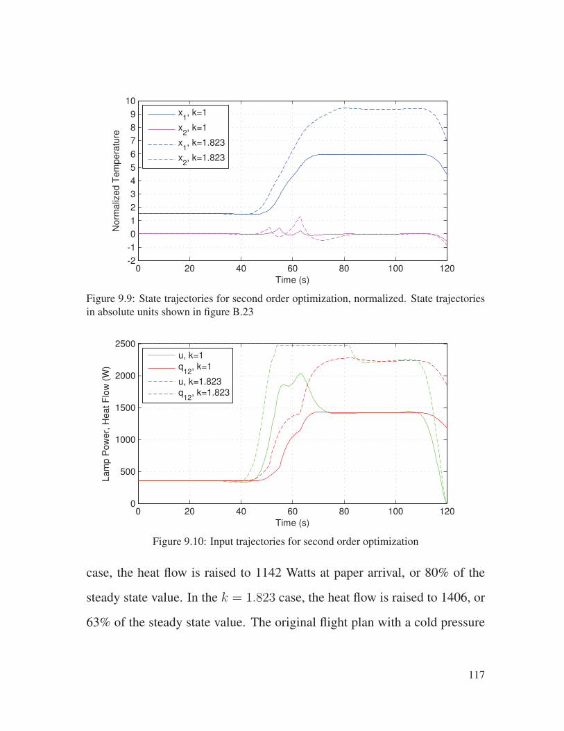
0 20 40 60 80 100 120-2
-1
0
1
2
3
4
5
6
7
8
9
10
Time (s)
Norm
aliz
ed T
em
pera
ture
x1, k=1
x2, k=1
x1, k=1.823
x2, k=1.823
Figure 9.9: State trajectories for second order optimization, normalized. State trajectories
in absolute units shown in figure B.23
0 20 40 60 80 100 1200
500
1000
1500
2000
2500
Time (s)
Lam
p P
ow
er,
Heat F
low
(W
)
u, k=1
q12
, k=1
u, k=1.823q
12, k=1.823
Figure 9.10: Input trajectories for second order optimization
case, the heat flow is raised to 1142 Watts at paper arrival, or 80% of the
steady state value. In the k = 1.823 case, the heat flow is raised to 1406, or
63% of the steady state value. The original flight plan with a cold pressure
117
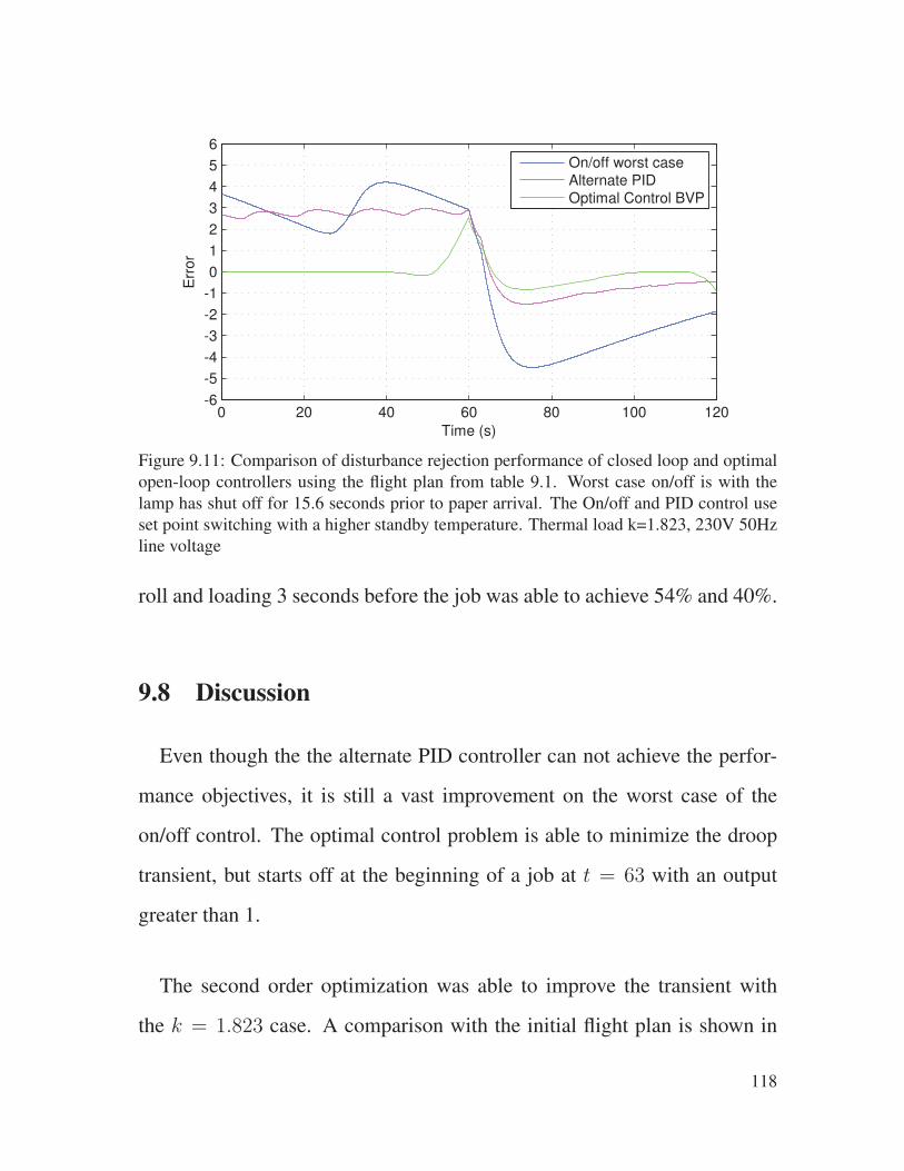
0 20 40 60 80 100 120-6
-5
-4
-3
-2
-1
0
1
2
3
4
5
6
Time (s)
Err
or
On/off worst case
Alternate PID
Optimal Control BVP
Figure 9.11: Comparison of disturbance rejection performance of closed loop and optimal
open-loop controllers using the flight plan from table 9.1. Worst case on/off is with the
lamp has shut off for 15.6 seconds prior to paper arrival. The On/off and PID control use
set point switching with a higher standby temperature. Thermal load k=1.823, 230V 50Hz
line voltage
roll and loading 3 seconds before the job was able to achieve 54% and 40%.
9.8 Discussion
Even though the the alternate PID controller can not achieve the perfor-
mance objectives, it is still a vast improvement on the worst case of the
on/off control. The optimal control problem is able to minimize the droop
transient, but starts off at the beginning of a job at t = 63 with an output
greater than 1.
The second order optimization was able to improve the transient with
the k = 1.823 case. A comparison with the initial flight plan is shown in
118
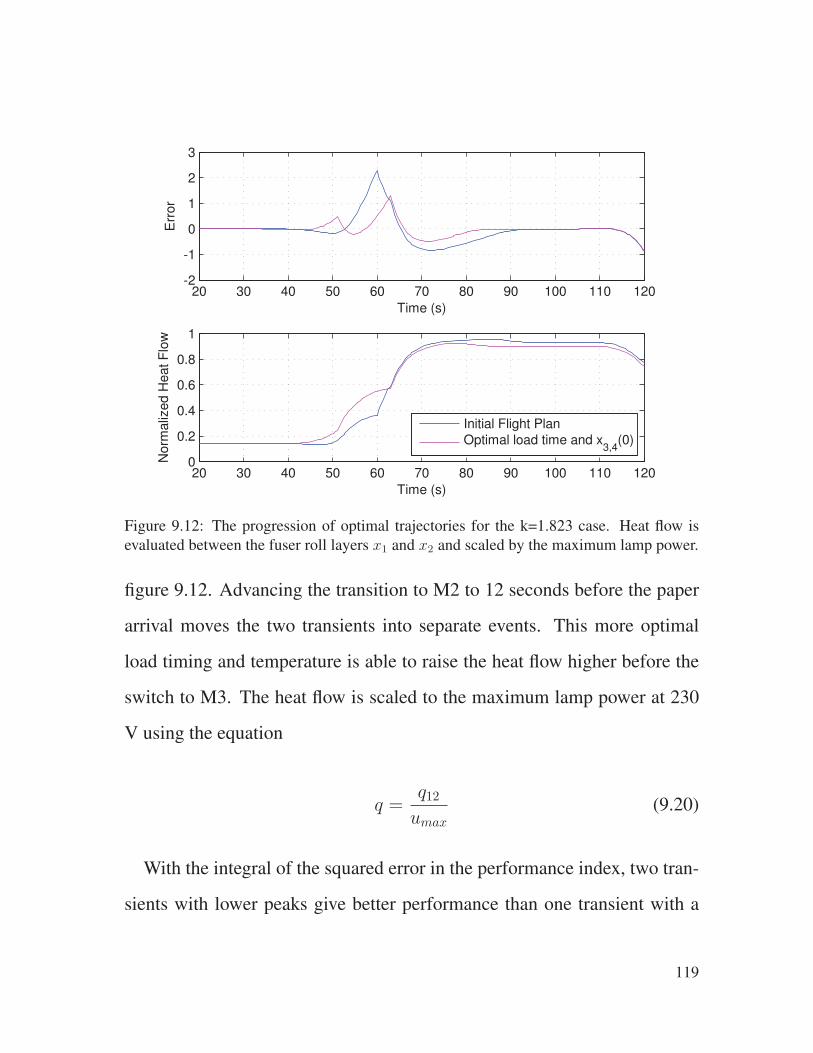
20 30 40 50 60 70 80 90 100 110 120-2
-1
0
1
2
3
Time (s)
Err
or
20 30 40 50 60 70 80 90 100 110 1200
0.2
0.4
0.6
0.8
1
Time (s)
Norm
aliz
ed H
eat F
low
Initial Flight Plan
Optimal load time and x3,4
(0)
Figure 9.12: The progression of optimal trajectories for the k=1.823 case. Heat flow is
evaluated between the fuser roll layers x1 and x2 and scaled by the maximum lamp power.
figure 9.12. Advancing the transition to M2 to 12 seconds before the paper
arrival moves the two transients into separate events. This more optimal
load timing and temperature is able to raise the heat flow higher before the
switch to M3. The heat flow is scaled to the maximum lamp power at 230
V using the equation
q =q12umax
(9.20)
With the integral of the squared error in the performance index, two tran-
sients with lower peaks give better performance than one transient with a
119

higher peak. If the fuser roll surface temperature during printing is what is
important, both cases give similar performance. Both outputs are slightly
higher than 1 at t = 63, but both keep the output above the lower limit of -1
afterwards.
120

Chapter 10
Controller Design
The solution to the optimal control problem found in the preceding chap-
ter allows some insight into how to better control the thermal system. Given
sufficient computing power and resources, a model predictive controller or
other form of numerical optimal controller could be implemented. This
would replicate the optimal trajectories in the previous chapter with a model
of the system in the controller. With finite computing resources of a con-
troller board on a production printer, a simplified feedforward system is
explored in this chapter to make a lightweight controller that achieves the
same end.
The key is to transition the thermal system from a low heat flow of 360
W in standby to a high heat flow when fusing media, 1600 to 2200 W. With
the trajectories known, a simple feedforward controller is implemented to
help execute this power transition before the media arrives at the fuser.
121

Table 10.1: Steady state values of the state
vector, x1 and x2 normalized to r2 and x3 and
x4 in degrees Celsius
Case x1 x2 x3 x4
M1 1.50 0 25 25
M2 1.93 0 187.5 187.5
M3 (k=1) 6.00 0 114.4 114.4
M3 (k=1.823) 9.43 0 102.0 102.0
In section 10.2, a control architecture is proposed to be able to parameter-
ize the desired behavior. Both the first order and second order optimization
of the optimal control input just barely miss achieving the performance ob-
jective of ±emax. The feedforward controller is designed to the fixed flight
plan with loading 3 seconds before the job, and the pressure roll tempera-
tures x3 and x4 are treated as a noise.
10.1 Trajectory Parameterization
In order to take advantage of the optimal trajectories, a lightweight con-
troller could use a parameterized or simplified form minimize space and
computing. For an arbitrary k, if the steady state power level required for
M3 is known, the desired steady state values of the states can be found and
the controller can move the states toward these values in advance of the
switch to M3. The steady state values are shown in table 10.1. Complete
table in temperature units can be found in section B.13.
122

0 20 40 60 80 100 120-2-101234567
k=1
Norm
aliz
ed T
em
pera
ture
0 20 40 60 80 100 1200
500
1000
1500
2000
2500
Time (s)
Pow
er
(W)
x1
x2
u
q12
Figure 10.1: The optimal state and input trajectory for k = 1, temperature normalized to the
fuser roll surface temperature.
The trajectory for the flight plan in section 9.5 for k = 1 is shown in
figure B.24. The fuser roll temperatures and heat flow stabilize in both the
idle and printing states. The stabilized initial state in M1 can be seen for t ∈
[0, 40] and the stabilized final state of the system is visible for t ∈ [80, 100].
The input stabilizes at 1500 W, along with the heat flow between the layers.
The heat flow between the fuser roll layers, q12 is a function of the dif-
ference between the states x1 and x2. The optimal solution increases the
core temperature by increasing the lamp input, while allowing the pressure
roll and paper load to decrease the surface temperature. A controller can
increase the core temperature in advance of the paper load arriving at the
123
fuser.
The desired value of the fuser roll core x1 can be determined from (5.1).
If x2 is to be kept constant, then x1 can be found algebraically by setting
x2 = 0
0 = (x1−x2)h1+(Tamb−x2)h1a+(x4−x2)h12r +(Tp−x2)h1pk (10.1)
Solving for x1:
x1 = −1
h1
[−h1x2 + (Tamb − x2)h1a + (x4 − x2)h12r + (Tp − x2)h1pk]
(10.2)
With the desired value of x1 known, the lamp input can be increased prior
to the job arrival to get the fuser roll core temperature toward this value.
With the appearance of the pressure roll surface temperature x4, this is not
a constant value.
As shown in figure 10.2, the initial and final values are now known, but a
smooth transition is needed between them. A prefilter can be used to soften
the transitions, making the reference smooth and continuous. To keep the
transitions smooth at both ends, a critically damped second order system is
used. This can be defined by the transfer function
124
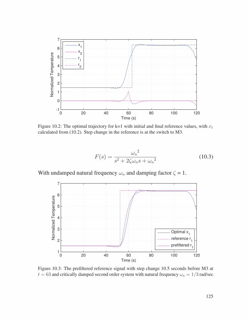
0 20 40 60 80 100 120-1
0
1
2
3
4
5
6
7
Time (s)
Norm
aliz
ed T
em
pera
ture
x1
x2
r1
r2
Figure 10.2: The optimal trajectory for k=1 with initial and final reference values, with x1
calculated from (10.2). Step change in the reference is at the switch to M3.
F (s) =ωn
2
s2 + 2ζωns+ ωn2
(10.3)
With undamped natural frequency ωn and damping factor ζ = 1.
0 20 40 60 80 100 1201
2
3
4
5
6
7
Time (s)
Norm
aliz
ed T
em
pera
ture
Optimal x1
reference r1
prefiltered r1
Figure 10.3: The prefiltered reference signal with step change 10.5 seconds before M3 at
t = 63 and critically damped second order system with natural frequency ωn = 1/3 rad/sec
125

LQR
Machine
Software
PrefilterReference
Generation
uFuser
Thermal
System-
+
Mode(t)
[Mode(t+th), k, r2]
r(t)
x
xd
ωωωωn
x4
FPC
q
Figure 10.4: The proposed block diagram for the feedforward control scheme. An advances
mode signal is required to be sent to the controller by horizon th, which will be used to makeset point changes prior to the switch to M3
With the natural frequency and the position in time adjustable, this new
reference signal can be tuned to match the desired trajectory of x1. A natural
frequency of ωn = 1/3 radians per second and advance time delay before
M3 td = 10.5 is shown in figure B.26. The delay and the natural frequency
can be adjusted for the range of k values. These values will be determined
in a later section.
10.2 Proposed control architecture
With the desired trajectories parameterized, the remaining control system
has to be constructed. With the reference trajectories able to be generated, a
model following controller is needed to track these reference signals.
126
The block diagram with the proposed system is shown in figure 10.4.
These elements will be developed in the next subsections.
• Machine software can provide a timing signal in advance of the mode
changes by a horizon th. In reality, the machine knows the transitions
between M1, M2, and M3 within milliseconds. Also needed are the k
values for particular media and the desired fuser roll surface tempera-
ture r2.
• The reference generator creates reference values r(t) for the states of
the fuser system. The reference can advance the actual mode switch
up to horizon th. Also provided is a time constant for the prefilter.
• The reference prefilter provides a continuous signal based on the steps
in reference input and adjustable natural frequency
• A hybrid linear quadratic regulator drives the system to follow the de-
sired trajectories, utilizing different gains based on the dynamic mode
• The fuser power controller FPC takes the desired power level u as an
input, and applies the current limiting and duty cycle constraints to
provide the applied power to the fuser q
To control the system with state feedback, the system must be observ-
able. With only the fuser roll surface temperature measured in the actual
system, the other states have to be estimated. The observability matrix can
be calculate for each of the dynamic states by the equation:
127
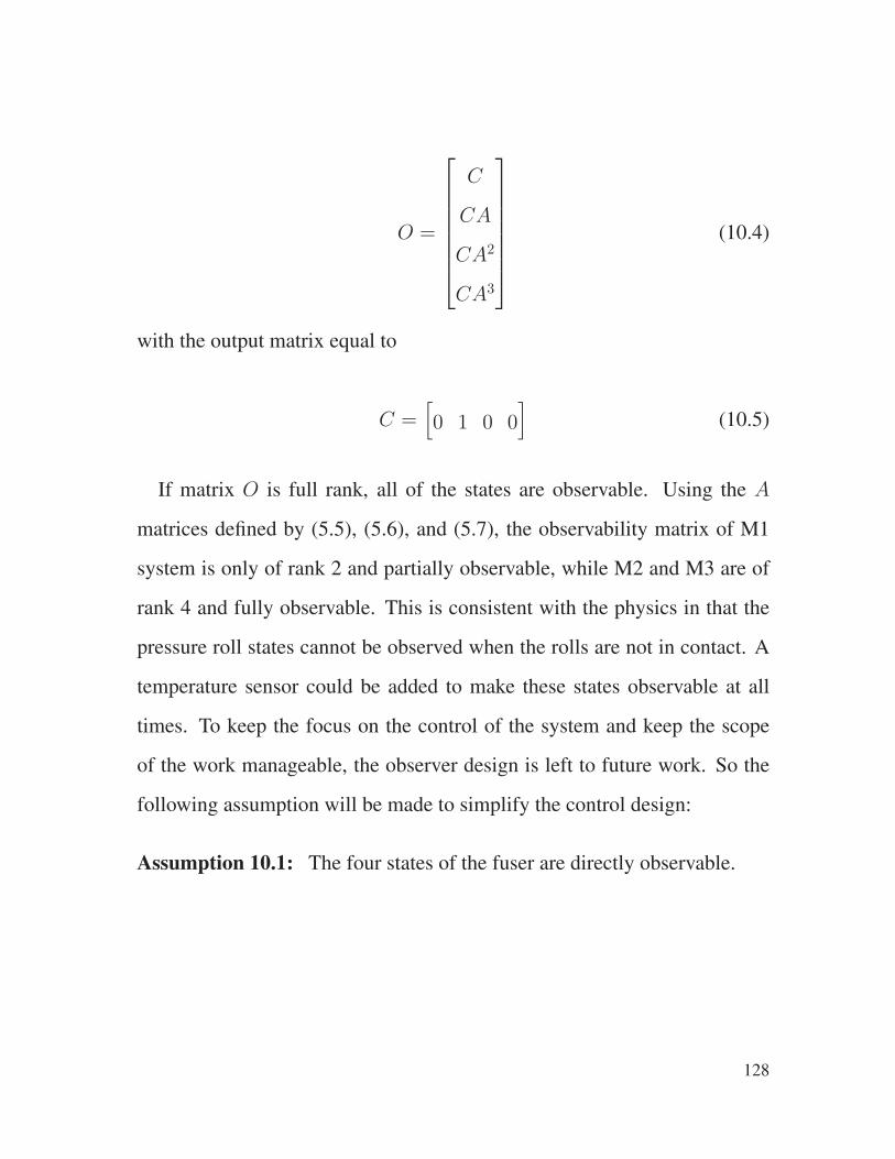
O =
C
CA
CA2
CA3
(10.4)
with the output matrix equal to
C =[
0 1 0 0]
(10.5)
If matrix O is full rank, all of the states are observable. Using the A
matrices defined by (5.5), (5.6), and (5.7), the observability matrix of M1
system is only of rank 2 and partially observable, while M2 and M3 are of
rank 4 and fully observable. This is consistent with the physics in that the
pressure roll states cannot be observed when the rolls are not in contact. A
temperature sensor could be added to make these states observable at all
times. To keep the focus on the control of the system and keep the scope
of the work manageable, the observer design is left to future work. So the
following assumption will be made to simplify the control design:
Assumption 10.1: The four states of the fuser are directly observable.
128
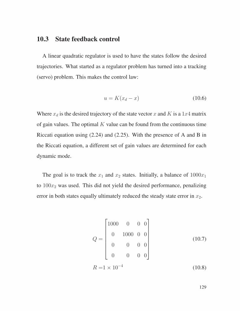
10.3 State feedback control
A linear quadratic regulator is used to have the states follow the desired
trajectories. What started as a regulator problem has turned into a tracking
(servo) problem. This makes the control law:
u = K(xd − x) (10.6)
Where xd is the desired trajectory of the state vector x andK is a 1x4matrix
of gain values. The optimalK value can be found from the continuous time
Riccati equation using (2.24) and (2.25). With the presence of A and B in
the Riccati equation, a different set of gain values are determined for each
dynamic mode.
The goal is to track the x1 and x2 states. Initially, a balance of 1000x1
to 100x2 was used. This did not yield the desired performance, penalizing
error in both states equally ultimately reduced the steady state error in x2.
Q =
1000 0 0 0
0 1000 0 0
0 0 0 0
0 0 0 0
(10.7)
R =1× 10⁻⁴ (10.8)
129
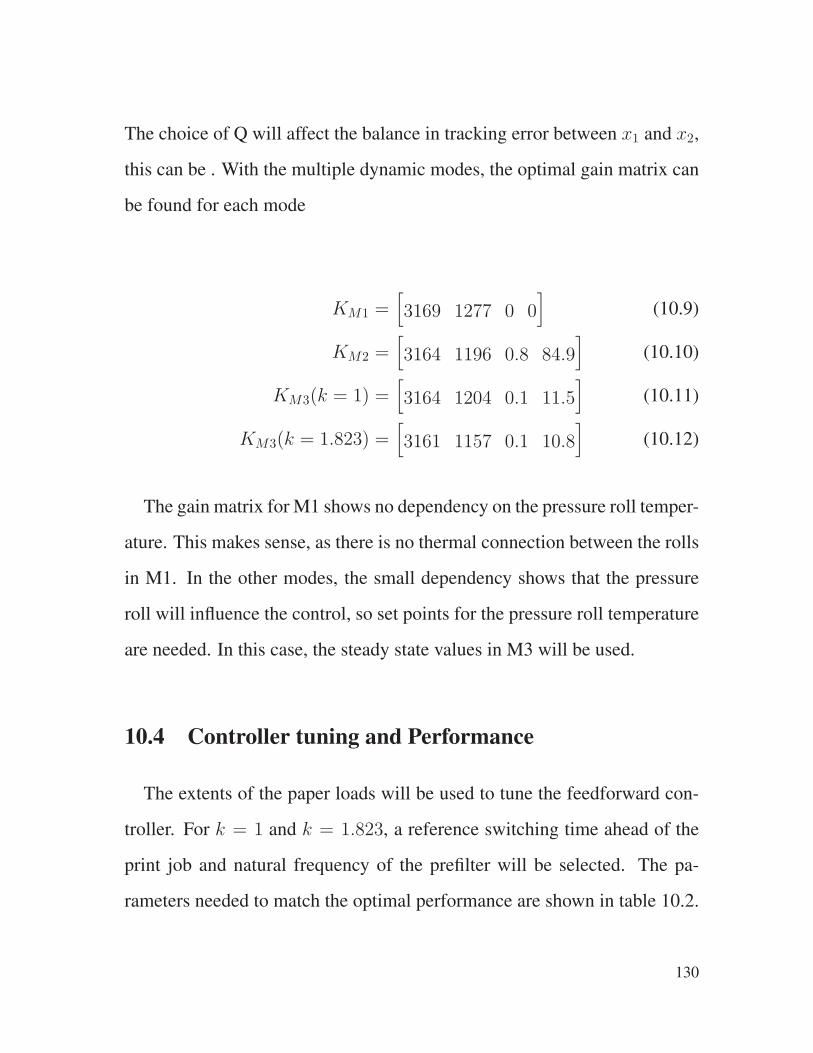
The choice of Q will affect the balance in tracking error between x1 and x2,
this can be . With the multiple dynamic modes, the optimal gain matrix can
be found for each mode
KM1 =[
3169 1277 0 0]
(10.9)
KM2 =[
3164 1196 0.8 84.9]
(10.10)
KM3(k = 1) =[
3164 1204 0.1 11.5]
(10.11)
KM3(k = 1.823) =[
3161 1157 0.1 10.8]
(10.12)
The gain matrix for M1 shows no dependency on the pressure roll temper-
ature. This makes sense, as there is no thermal connection between the rolls
in M1. In the other modes, the small dependency shows that the pressure
roll will influence the control, so set points for the pressure roll temperature
are needed. In this case, the steady state values in M3 will be used.
10.4 Controller tuning and Performance
The extents of the paper loads will be used to tune the feedforward con-
troller. For k = 1 and k = 1.823, a reference switching time ahead of the
print job and natural frequency of the prefilter will be selected. The pa-
rameters needed to match the optimal performance are shown in table 10.2.
130
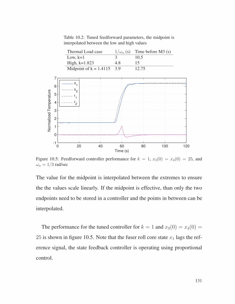
Table 10.2: Tuned feedforward parameters, the midpoint is
interpolated between the low and high values
Thermal Load case 1/ωn (s) Time before M3 (s)
Low, k=1 3 10.5
High, k=1.823 4.8 15
Midpoint of k = 1.4115 3.9 12.75
0 20 40 60 80 100 120-1
0
1
2
3
4
5
6
7
Time (s)
Norm
aliz
ed T
em
pera
ture
x1
x2
r1
r2
Figure 10.5: Feedforward controller performance for k = 1, x3(0) = x4(0) = 25, andωn = 1/3 rad/sec
The value for the midpoint is interpolated between the extremes to ensure
the the values scale linearly. If the midpoint is effective, than only the two
endpoints need to be stored in a controller and the points in between can be
interpolated.
The performance for the tuned controller for k = 1 and x3(0) = x4(0) =
25 is shown in figure 10.5. Note that the fuser roll core state x1 lags the ref-
erence signal, the state feedback controller is operating using proportional
control.
131
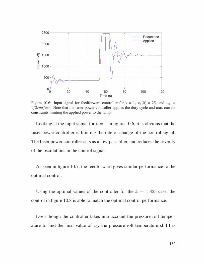
0 20 40 60 80 100 1200
500
1000
1500
2000
2500
Time (s)
Pow
er
(W)
Requested
Applied
Figure 10.6: Input signal for feedforward controller for k = 1, x4(0) = 25, and ωn =1/3rad/sec. Note that the fuser power controller applies the duty cycle and max currentconstraints limiting the applied power to the lamp.
Looking at the input signal for k = 1 in figure 10.6, it is obvious that the
fuser power controller is limiting the rate of change of the control signal.
The fuser power controller acts as a low-pass filter, and reduces the severity
of the oscillations in the control signal.
As seen in figure 10.7, the feedforward gives similar performance to the
optimal control.
Using the optimal values of the controller for the k = 1.823 case, the
control in figure 10.8 is able to match the optimal control performance.
Even though the controller takes into account the pressure roll temper-
ature to find the final value of x1, the pressure roll temperature still has
132

0 20 40 60 80 100 120
-0.5
0
0.5
1
Time (s)
Scale
d O
utp
ut
PR Temp = 25, k = 1, Td = 10.5, 1/Wn = 3
Optimal
Feedforward
Figure 10.7: Controller comparison to optimal solution with x3(0) = x4(0) = 25
0 20 40 60 80 100 120-1
-0.5
0
0.5
1
1.5
2
2.5
3
Time (s)
Scale
d O
utp
ut
PR Temp = 25, k = 1.823, Td = 15, 1/Wn = 4.8
Optimal
Feedforward
Figure 10.8: Feedforward controller performance for k = 1.823, and x3(0) = x4(0) = 25
133
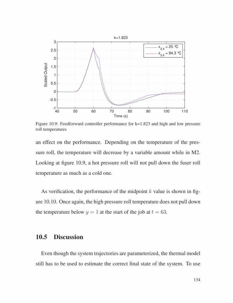
40 50 60 70 80 90 100 110-1
-0.5
0
0.5
1
1.5
2
2.5
3S
cale
d O
utp
ut
Time (s)
k=1.823
x3,4
= 25 °C
x3,4
= 94.3 °C
Figure 10.9: Feedforward controller performance for k=1.823 and high and low pressure
roll temperatures
an effect on the performance. Depending on the temperature of the pres-
sure roll, the temperature will decrease by a variable amount while in M2.
Looking at figure 10.9, a hot pressure roll will not pull down the fuser roll
temperature as much as a cold one.
As verification, the performance of the midpoint k value is shown in fig-
ure 10.10. Once again, the high pressure roll temperature does not pull down
the temperature below y = 1 at the start of the job at t = 63.
10.5 Discussion
Even though the system trajectories are parameterized, the thermal model
still has to be used to estimate the correct final state of the system. To use
134
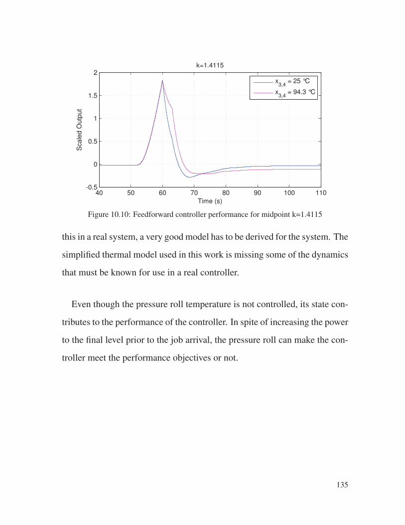
40 50 60 70 80 90 100 110-0.5
0
0.5
1
1.5
2S
cale
d O
utp
ut
Time (s)
k=1.4115
x3,4
= 25 °C
x3,4
= 94.3 °C
Figure 10.10: Feedforward controller performance for midpoint k=1.4115
this in a real system, a very good model has to be derived for the system. The
simplified thermal model used in this work is missing some of the dynamics
that must be known for use in a real controller.
Even though the pressure roll temperature is not controlled, its state con-
tributes to the performance of the controller. In spite of increasing the power
to the final level prior to the job arrival, the pressure roll can make the con-
troller meet the performance objectives or not.
135

Chapter 11
Conclusions and Future Work
11.1 Conclusions
11.1.1 Complete Thermo-electric Model
Assembling the thermal model with the control as implemented in Nuvera
yielded some insights into the behavior, and more importantly replicated the
limit cycles seen in the existing system. This was further aggravated when
adding the fuser power controller.
11.1.2 Optimal Control
The optimal control boundary value problem led into insights into how to
transition the fuser from a low power state to a high power state. With
knowledge of how the system responds to the input, the control was in-
creased at a slow enough rate to meet the fuser power controller constraints
136

and meet the flicker constraints. The second level optimization was able to
find a set of conditions to maximize on the performance objective, but only
marginally improved the control, and did not meet the objective at the start
of the job.
11.1.3 Control Design
The attempt at designing a feedforward controller still required knowledge
about the desired power state of the fuser. The pressure roll temperature was
significant enough to make the control not meet the performance objectives.
However, the feedforward controller was able to replicate the performance
of the optimal control trajectories and be able to execute real-time.
11.2 Suggestions for future work
11.2.1 Thermal Modeling
The model developed for this work was simplified so the high bandwidth
droop transient was not captured precisely. Using a model with more states
or delays can improve the tracking of this model.
With assumption 5.1, the relationship of the heat transfer coefficients be-
tween the rolls and the media was assumed. Further identification of these
parameters for various media will extend the fidelity of the model and may
137

lead to other insights into control based on media. A higher fidelity model
may also lead to the ability to estimate the states of interest, especially the
fuser roll core.
The pressure roll temperature is not measured in some printers. Using
a high fidelity model as in those above may lead to an effective observer
for pressure roll temperature. With the pressure roll intermittently loaded in
standby between M1 and M2, the temperature could be estimated while the
roll is in contact. This is similar to the shared sensing/actuation in [7].
The link between the fuser roll core temperature and the ambient temper-
ature of the lamp model was not made. This may require an additional state
being the air temperature around the lamp. Some additional system identi-
fication could find this linkage and lead to a better thermo-electric model.
11.2.2 Power System Modeling
The power system was only exercised for line voltages of 208 and 230
volts. In reality, the line voltage can vary from 180 to 264 volts. In addition,
there are multiple lamp power ratings that are used across this range. One
phenomenon of interest is the stall that happens with the 2200 watt lamp
used in this work running with the fuser power controller at 264 volts. The
fuser power controller cannot put in enough power at the low duty cycles to
heat the lamp so it finds an equilibrium condition where it will not increase
138

to full power.
Typically, production printers run off three-phase power. In this work a
single lamp is used between two phases in the 60 Hz case, and one phase
and neutral for the 50 Hz case. Some of the MIMO fusing systems require
connecting multiple lamps between all three phases of the power system.
This is further complicated as 60 Hz uses a delta load connection, and 50
Hz uses a wye connection of the loads. Understanding the flicker impact of
the lamps in these systems is not trivial.
11.2.3 Control
Other disturbances are present in the system that could be addressed.
There is disturbance when the printer switches media while printing, caus-
ing a step change in the sliding load variable k. In addition, there is an
overshoot at the end of a job when switching from a high to low thermal
load. The image quality is not impacted by this temperature. Control meth-
ods to keep the standby temperature low could also be examined.
The optimal control problem may be improved by altering the cost func-
tional to penalize tracking error more when in M3. Using a step change was
tried, but led to undesired results.
139

The optimal open loop control performance should be verified on an ac-
tual system. This would require rework of the fuser power controller to give
direct access to the PWM duty cycle electronically or though the firmware.
This may lead to a different architecture of a future system to integrate the
control. In addition, a model predictive controller could be used to incorpo-
rate a high fidelity model to anticipate the transients similar to the optimal
control boundary value problem.
140

Bibliography
[1] Nuvera paper path controller (PPC) temperature control source code.
source code, 2006.
[2] Matlab, 2009.
[3] Anonymous. Electromagnetic compatibility: Limitations of voltage
changes, voltage fluctuations and flicker in public low-voltage supply
systems, for equipment with rated current ≤ 16 A per phase and not
subject to conditional connection. IEC Standard IEC 61000-3-3, Inter-
national Electrotechnical Commission, 2002.
[4] Anonymous. Electromagnetic compatibility (EMC), testing and mea-
surement techniques, flickermeter. functional and design specifica-
tions. IEC Standard IEC 61000-4-15, International Electrotechnical
Commission, 2003.
[5] Andrea Berlola, George Cristian Lnraroiu, Mariacriitina Roscia, and
Dsrio Zaninelli. A matlab-simulink flickermeter model for power qual-
ity studies. In 11th International Conference on Harmonics and Qual-
ity of Power.
[6] Eduardo F. Camacho and Carlos Bordons. Model Predictive Control.
[7] Tuhin Das and Ranjan Mukherjee. Shared-sensing and control using
reversible transducers. IEEE Transactions on control systems technol-
ogy, 17(1):242–248, January 2009.
141
[8] Yongsoon Eun. Modeling for systems analysis and controller synthe-
sis: ****** fuser. Xerox internal report, 2005.
[9] Yongsoon Eun, Eric Hamby, Charles Facchini, and Jeffrey Swing.
Modeling Nuvera Fuser for Controller Optimization. Xerox internal
report, 2007.
[10] Charles Facchini. Flicker characteristics analysis. Xerox Internal Re-
port, 2008.
[11] Donald G. Fink and H. Wayne Beaty, editors. Standard Handbook for
electrical engineers. McGraw-Hill, fourteenth edition, 1999.
[12] Paul Fromm and Don Bott. Fusing technologies in electrophotographic
systems. Xerox internal report, 2005.
[13] Debbie Gualtieri and Glenn Batchelor. Temperature and power mea-
surements during print runs on nuvera machine 259. Xerox internal
report, 2005.
[14] B. Mark Hirst. Reduced flicker fusing system for use in electrophoto-
graphic printers and copiers. United States Patent 5,789,723, August
1998.
[15] Frank P. Incropera and David P. DeWitt. Introduction to Heat Transfer.
John Wiley & Sons, third edition, 1996.
[16] Patrik Jourdan. Open source flicker measurement-simulator.
http://www.solcept.ch/en/embedded-tools/
flickersim.html, 2003.
[17] Hassan K. Khalil. Nonlinear systems. Macmillian Publishing Group,
1992.
142
[18] Donald E. Kirk. Optimal control theory, an Introduction. Dover Pub-
lications, Inc., 1970.
[19] Frank L. Lewis and Vassilis L. Syrmos. Optimal Control. Wiley-
Interscience, second edition, 1995.
[20] Feng Liu, Donald Bott, Yongsoon Eun, Eric Hamby, and Faming Li.
Control oriented modeling for iGen3 fusing.
[21] Masataka Maeda and Manabu Takeuchi. A Simulation Model for Es-
timation of Flicker Levels Induced by On-Off Switching of a Halogen
Heater of a LBP Fuser. In NIP21: 21st International Conference on
Digital Printing Technologies Final Program and Proceedings, pages
618–622. Society for Imaging Science and Technology, 2005.
[22] International Rectifier. Insulated gate bipolar transistor with ultrafast
soft recovery diode. Drawing IRGP30B120KD-EP, 2004.
[23] M. M. Peretz S. Ben-Yaakov and B. Hesterman. A SPICE compatible
behavioral electrical model of a heated tungsten filament. In Confer-
ence Proceedings - IEEE Applied Power Electronics Conference and
Exposition - APEC, volume 2, pages 1079–1084, 2005.
[24] Sigurd Skogestad and Ian Postlethwaite. Multivariable Feedback Con-
trol: Analysis and Design. John Wiley & Sons, second edition, 2005.
[25] Gregory Weselak. Fuser Power Controller (FPC) Module Operating
Description, 2006.
[26] Gregory Weselak. Fuser power controller schematic. Xerox Drawing
156P19747, 2007.
143

[27] Z. Zhou, M.S. Khanniche, P. Igic, S.T. Kong, M. Towers, and P.A.
Mawby. A fast power loss calculation method for long real time ther-
mal simulation of IGBT modules for a three-phase inverter system. In
IEEE 11th European Conference on Power Electronics and Applica-
tions, 2005.
144
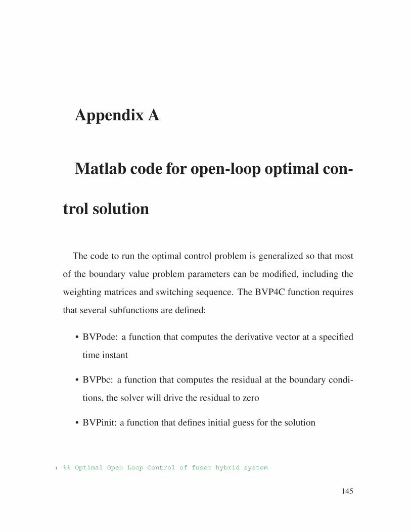
Appendix A
Matlab code for open-loop optimal con-
trol solution
The code to run the optimal control problem is generalized so that most
of the boundary value problem parameters can be modified, including the
weighting matrices and switching sequence. The BVP4C function requires
that several subfunctions are defined:
• BVPode: a function that computes the derivative vector at a specified
time instant
• BVPbc: a function that computes the residual at the boundary condi-
tions, the solver will drive the residual to zero
• BVPinit: a function that defines initial guess for the solution
1 %% Optimal Open Loop Control of fuser hybrid system
145
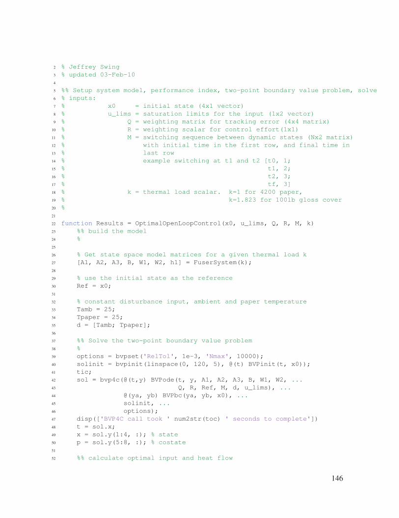
2 % Jeffrey Swing
3 % updated 03-Feb-10
4
5 %% Setup system model, performance index, two-point boundary value problem, solve
6 % inputs:
7 % x0 = initial state (4x1 vector)
8 % u_lims = saturation limits for the input (1x2 vector)
9 % Q = weighting matrix for tracking error (4x4 matrix)
10 % R = weighting scalar for control effort(1x1)
11 % M = switching sequence between dynamic states (Nx2 matrix)
12 % with initial time in the first row, and final time in
13 % last row
14 % example switching at t1 and t2 [t0, 1;
15 % t1, 2;
16 % t2, 3;
17 % tf, 3]
18 % k = thermal load scalar. k=1 for 4200 paper,
19 % k=1.823 for 100lb gloss cover
20 %
21
22 function Results = OptimalOpenLoopControl(x0, u_lims, Q, R, M, k)
23 %% build the model
24 %
25
26 % Get state space model matrices for a given thermal load k
27 [A1, A2, A3, B, W1, W2, h1] = FuserSystem(k);
28
29 % use the initial state as the reference
30 Ref = x0;
31
32 % constant disturbance input, ambient and paper temperature
33 Tamb = 25;
34 Tpaper = 25;
35 d = [Tamb; Tpaper];
36
37 %% Solve the two-point boundary value problem
38 %
39 options = bvpset('RelTol', 1e-3, 'Nmax', 10000);
40 solinit = bvpinit(linspace(0, 120, 5), @(t) BVPinit(t, x0));
41 tic;
42 sol = bvp4c(@(t,y) BVPode(t, y, A1, A2, A3, B, W1, W2, ...
43 Q, R, Ref, M, d, u_lims), ...
44 @(ya, yb) BVPbc(ya, yb, x0), ...
45 solinit, ...
46 options);
47 disp(['BVP4C call took ' num2str(toc) ' seconds to complete'])
48 t = sol.x;
49 x = sol.y(1:4, :); % state
50 p = sol.y(5:8, :); % costate
51
52 %% calculate optimal input and heat flow
146
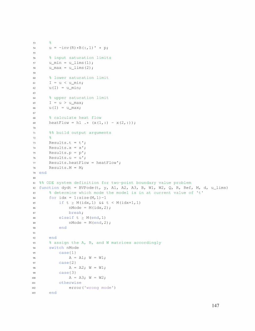
53 %
54 u = -inv(R)*B(:,1)' * p;
55
56 % input saturation limits
57 u_min = u_lims(1);
58 u_max = u_lims(2);
59
60 % lower saturation limit
61 I = u < u_min;
62 u(I) = u_min;
63
64 % upper saturation limit
65 I = u > u_max;
66 u(I) = u_max;
67
68 % calculate heat flow
69 heatFlow = h1 .* (x(1,:) - x(2,:));
70
71 %% build output arguments
72 %
73 Results.t = t';
74 Results.x = x';
75 Results.p = p';
76 Results.u = u';
77 Results.heatFlow = heatFlow';
78 Results.M = M;
79 end
80
81 %% ODE system definition for two-point boundary value problem
82 function dydt = BVPode(t, y, A1, A2, A3, B, W1, W2, Q, R, Ref, M, d, u_lims)
83 % determine which mode the model is in at current value of 't'
84 for idx = 1:size(M,1)-1
85 if t ≥ M(idx,1) && t < M(idx+1,1)
86 nMode = M(idx,2);
87 break;
88 elseif t ≥ M(end,1)
89 nMode = M(end,2);
90 end
91
92 end
93 % assign the A, B, and W matrices accordingly
94 switch nMode
95 case1
96 A = A1; W = W1;
97 case2
98 A = A2; W = W1;
99 case3
100 A = A3; W = W2;
101 otherwise
102 error('wrong mode')
103 end
147

104
105 % calculate u from stationary condition
106 u = -inv(R)* B' * y(5:8);
107
108 % enforce input constraints
109 u_min = u_lims(1); u_max = u_lims(2);
110
111 if u ≤ u_min
112 u = u_min;
113 elseif u ≥ u_max
114 u = u_max;
115 end
116
117 % assemble derivative vector
118 xdot = A*y(1:4) + B*u + W*d;
119 pdot = [-Q, -A'] * y + Q * Ref;
120 dydt = [xdot;
121 pdot];
122 end
123
124 %% boundary condition function
125 function res = BVPbc(ya, yb, x0)
126 res = [ya(1:4) - x0;
127 yb(5:8)];
128 end
129
130 %% initialization function
131 function v = BVPinit(t, x0)
132 v = [x0; [0;0;0;0]];
133 end
148