minimizing sum of truncated convex functions and its ... · ing variable selection, outlier...
TRANSCRIPT
Minimizing Sum of Truncated ConvexFunctions and Its Applications
Tzu-Ying Liu and Hui Jiang∗
Department of Biostatistics, University of MichiganAnn Arbor, MI 48105
June 28, 2017
Abstract
In this paper, we study a class of problems where the sum of truncated convexfunctions is minimized. In statistical applications, they are commonly encounteredwhen `0-penalized models are fitted and usually lead to NP-Hard non-convex opti-mization problems. In this paper, we propose a general algorithm for the global mini-mizer in low-dimensional settings. We also extend the algorithm to high-dimensionalsettings, where an approximate solution can be found efficiently. We introduce sev-eral applications where the sum of truncated convex functions is used, compare ourproposed algorithm with other existing algorithms in simulation studies, and showits utility in edge-preserving image restoration on real data.
Keywords: `0 penalty; NP-Hard; non-convex optimization; sum of truncated convex func-tions; outlier detection; signal and image restoration;
∗Please send all correspondence to [email protected].
1
arX
iv:1
608.
0023
6v3
[st
at.C
O]
27
Jun
2017

1 Introduction
Regularization methods in statistical modeling have gain popularity in many fields, includ-
ing variable selection, outlier detection, and signal processing. Recent studies (Shen et al.,
2012; She and Owen, 2012) have shown that models with non-convex penalties possess su-
perior performance compared with those with convex penalties. While the latter in general
can be obtained with ease by virtue of many well-developed methods for convex optimiza-
tion (Boyd and Vandenberghe, 2004), there are limited options in terms of global solutions
for non-convex optimization, which are more and more commonly encountered in modern
statistics and engineering. Current approaches often rely on convex relaxation (Candes
and Tao, 2010), local solutions by iterative algorithms (Fan and Li, 2001) or trading time
for global optimality with stochastic search (Zhigljavsky and Zilinskas, 2007).
In this paper, we study a special class of non-convex optimization problems, for which
the objective function can be written as a sum of truncated convex functions. That is,
x = arg minx
n∑i=1
min{fi(x), λi}, (1)
where fi : Rd → R, i = 1, . . . , n, are convex functions and the truncated levels λi ∈ R, i =
1, . . . , n, are constants. Due to the truncation of fi(·) at λi, the objective function is often
non-convex. See Figure 1 for an example.
While in general such problems are NP-Hard (see Section 3 for formal results), we
show that for some fi(·) there is a polynomial-time algorithm for the global minimizer in
low-dimensional settings. The idea is simple: When the objective function is piecewise
convex (e.g., see Figure 1), we can partition the domain so that the objective function
becomes convex when restricted to each piece. This way, we can find the global minimizer
by enumerating all the pieces, minimizing the objective function on each piece, and taking
the minimum among all local minima.
The rest of the paper is organized as follows. In Section 2, we demonstrate the utility
of our algorithm in several applications where the objective function can be transformed
into a sum of truncated convex functions. In Section 3, we lay out the general algorithm
for the global solution and its implementation in low-dimensional settings. As we will see
in the complexity analysis, the running time grows exponentially with the number of di-
2
−2 −1 0 1 2 30
24
68
x
f
f1 + f2f1f2
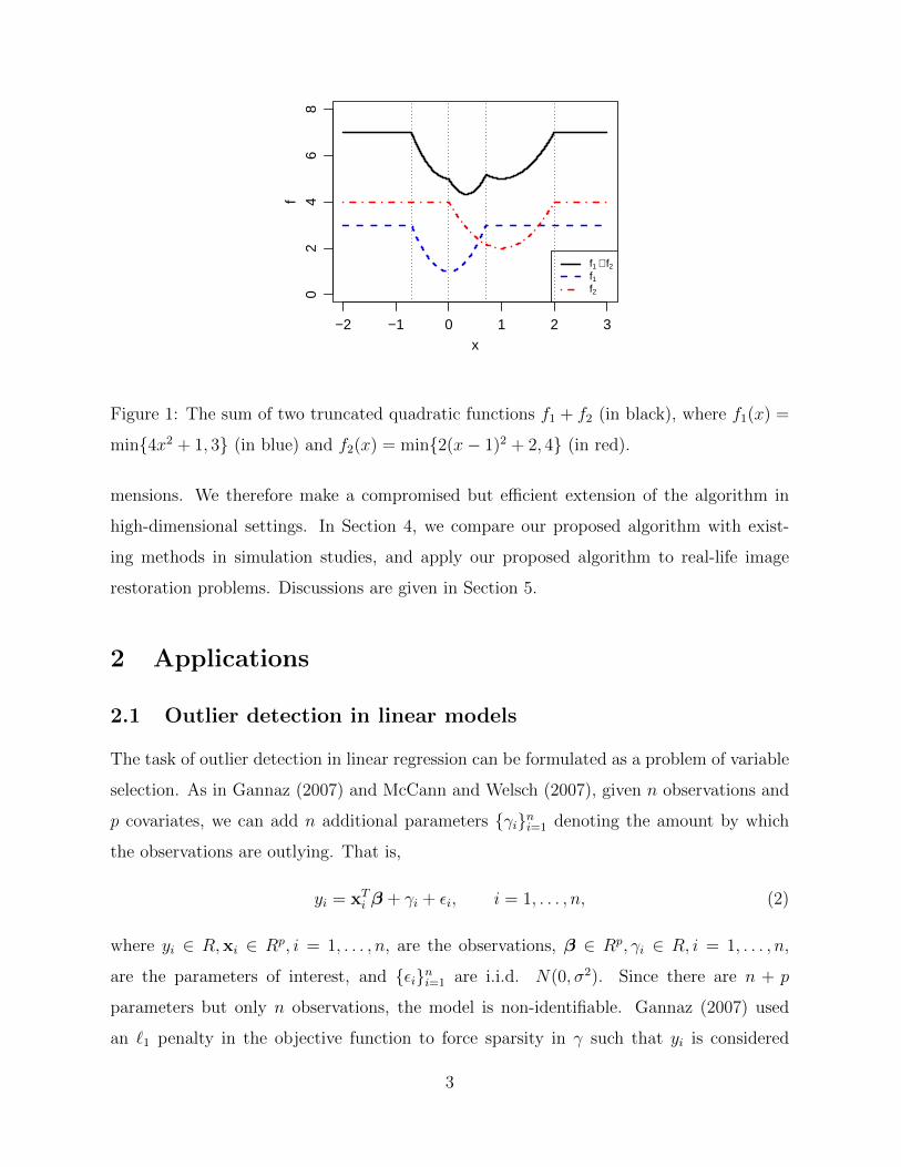
Figure 1: The sum of two truncated quadratic functions f1 + f2 (in black), where f1(x) =
min{4x2 + 1, 3} (in blue) and f2(x) = min{2(x− 1)2 + 2, 4} (in red).
mensions. We therefore make a compromised but efficient extension of the algorithm in
high-dimensional settings. In Section 4, we compare our proposed algorithm with exist-
ing methods in simulation studies, and apply our proposed algorithm to real-life image
restoration problems. Discussions are given in Section 5.
2 Applications
2.1 Outlier detection in linear models
The task of outlier detection in linear regression can be formulated as a problem of variable
selection. As in Gannaz (2007) and McCann and Welsch (2007), given n observations and
p covariates, we can add n additional parameters {γi}ni=1 denoting the amount by which
the observations are outlying. That is,
yi = xTi β + γi + εi, i = 1, . . . , n, (2)
where yi ∈ R,xi ∈ Rp, i = 1, . . . , n, are the observations, β ∈ Rp, γi ∈ R, i = 1, . . . , n,
are the parameters of interest, and {εi}ni=1 are i.i.d. N(0, σ2). Since there are n + p
parameters but only n observations, the model is non-identifiable. Gannaz (2007) used
an `1 penalty in the objective function to force sparsity in γ such that yi is considered
3

an outlier if γi 6= 0 and an observation conforming to the assumed distribution if γi = 0.
McCann and Welsch (2007) treated (2) as a variable selection problem and applied the Least
Angle Regression. Similar idea for outlier detection has also been used for robust Lasso
regression (Nasrabadi et al., 2011; Katayama and Fujisawa, 2015), Poisson regression (Jiang
and Salzman, 2015), logistic regression (Tibshirani and Manning, 2014), clustering (Witten,
2013; Georgogiannis, 2016), as well as a large class of regression and classification problems
intoduced in Lee et al. (2012).
She and Owen (2012) took into consideration the issues of masking and swamping when
there are multiple outliers in the data. By definition, masking refers to the situation when
a true outlier is not detected because of other outliers. Swamping, on the other hand, refers
to the situation when an observation conforming to the assumed distribution is considered
outlying under the influence of true outliers. They pointed out that using the `0 penalty
instead of the `1 penalty in the objective function could resolve both issues. Assuming σ
is known, adding an `0 penalty to the negative log-likelihood function for model (2), the
objective function becomes
f(β,γ) =n∑i=1
(yi − xTi β − γi)2 + λn∑i=1
1(γi 6= 0), (3)
where λ is a tuning parameter and 1(·) is the indicator function. It can be shown that this
problem can be solved by minimizing a sum of truncated quadratic functions.
Proposition 2.1. Minimizing (3) in β and γ jointly is equivalent to minimizing the fol-
lowing sum of truncated quadratic functions in β
g(β) =n∑i=1
min{(yi − xTi β)2, λ}.
This result is consistent with the proposition by She and Owen (2012) that the estimate
β from minimizing (3) is an M -estimate associated with the skipped-mean loss. Since the
objective function is non-convex, She and Owen (2012) proposed an iterative hard thresh-
olding algorithm named Θ-IPOD (iterative procedure for outlier detection) to minimize it.
Similar to other iterative procedures, Θ-IPOD only guarantees local solutions. A simula-
tion study comparing our proposed algorithm with Θ-IPOD and several other robust linear
4
regression algorithms is presented in Section 4.1. We implement the Θ-IPOD algorithm in
R (see Supplementary Algorithm S5 for details).
Furthermore, Proposition 2.1 can be extended to the class of generalized linear models
(GLMs). Suppose that Yi ∈ R, i = 1, . . . , n, follow a distribution in the exponential family,
f(Yi = yi|θi, φ) = exp
{yiθi − b(θi)
a(φ)+ c(yi, φ)
},
where θi is the canonical parameter and φ is the dispersion parameter (assumed known
here). For a GLM with canonical link function g, θi = g(µi) = xTi β + γi, the `0-penalized
negative log-likelihood function is
f(β,γ) =n∑i=1
{b(xTi β + γi)− (xTi β + γi)yi}+ λn∑i=1
1(γi 6= 0). (4)
It can be shown that minimizing (4) is equivalent to minimizing a sum of truncated convex
functions.
Proposition 2.2. Minimizing (4) in β and γ jointly is equivalent to minimizing the fol-
lowing function in β
g(β) =n∑i=1
min{b(xTi β)− (xTi β)yi, λ∗i },
where λ∗i = b(g(yi)) − g(yi)yi + λ, i = 1, . . . , n, are constants. Since b is convex (Agarwal
and Daume III, 2011), the above is a sum of truncated convex function.
Example 2.3. Suppose that {Yi}ni=1 follow Poisson distributions with mean {µi}ni=1, re-
spectively, and that g(µi) = log µi = xTi β + γi, where γi = 0 if yi conforms to the assumed
distribution and γi 6= 0 if yi is an outlier. The `0-penalized negative log-likelihood function
is
f(β,γ) =n∑i=1
{ex
Ti β+γi − (xTi β + γi)yi
}+ λ
n∑i=1
1(γi 6= 0). (5)
According to Proposition 2.2, minimizing (5) is equivalent to minimizing the following
function
g(β) =n∑i=1
min{exTi β − (xTi β)yi, λ
∗i }, where λ∗i = λ− yi log yi + yi,
which is a sum of truncated convex functions.
5
2.2 Convex shape placement
Given a convex shape S ⊂ Rd, and n points pi ∈ Rd, i = 1, . . . , n, each associated with
weight wi > 0, the problem of finding a translation of S such that the total weight of
the points contained in S is maximized has applications in the placement of facilities or
resources such as radio stations, power plants or satellites (Mehrez and Stulman, 1982).
For some simple shapes (e.g., circles or polygons) in low-dimensional settings, this problem
has been well studied (Chazelle and Lee, 1986; Barequet et al., 1997).
We show that this problem can be solved by minimizing a sum of truncated convex
functions. Without loss of generality, let S0 ⊂ Rd denote the region covered by S when it
is placed at the origin. Here the location of S can be defined as the location of its centroid.
For each point pi, let Si ⊂ Rd be the set of locations for placing S such that it covers pi.
It is easy to see that Si = {x : pi − x ∈ S0} = {pi − y : y ∈ S0}, and that the shape of Si
is simply a mirror image of S0 and therefore it is also convex. Furthermore, define convex
function fi : Rd → R as
fi(x) =
−wi if x ∈ Si,
∞ otherwise.
Then the optimal placement of S can be found by minimizing the sum of truncated convex
functions∑n
i=1 min{fi(x), λi} as in (1) where λi = 0, i = 1, . . . , n.
Some examples of this application are given in Section 4.3.
2.3 Signal and image restoration
Signal restoration aims to recover the original signal from observations corrupted by noise.
Suppose that the observed data y are generated from the original data x following the
model (Portilla et al., 2015):
y = Hx + ε
where H is a matrix performing some linear transformation on the data (e.g., smoothing)
and ε is the vector the measurement errors, often modeled as additive white Gaussian noise
(AWGN). The goal is to estimate (a.k.a. restore or reconstruct) x from observed y and
a known H. When both x and y are (vectorized) images, the problem is called image
restoration.
6
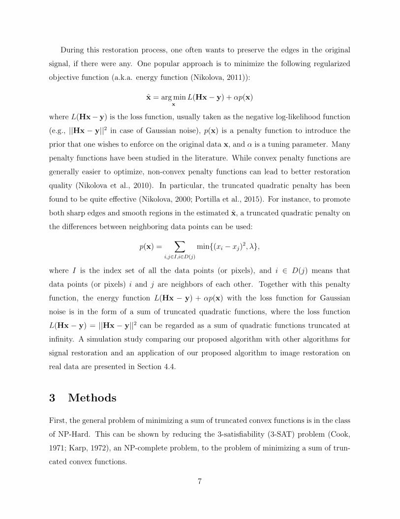
During this restoration process, one often wants to preserve the edges in the original
signal, if there were any. One popular approach is to minimize the following regularized
objective function (a.k.a. energy function (Nikolova, 2011)):
x = arg minx
L(Hx− y) + αp(x)
where L(Hx− y) is the loss function, usually taken as the negative log-likelihood function
(e.g., ||Hx − y||2 in case of Gaussian noise), p(x) is a penalty function to introduce the
prior that one wishes to enforce on the original data x, and α is a tuning parameter. Many
penalty functions have been studied in the literature. While convex penalty functions are
generally easier to optimize, non-convex penalty functions can lead to better restoration
quality (Nikolova et al., 2010). In particular, the truncated quadratic penalty has been
found to be quite effective (Nikolova, 2000; Portilla et al., 2015). For instance, to promote
both sharp edges and smooth regions in the estimated x, a truncated quadratic penalty on
the differences between neighboring data points can be used:
p(x) =∑
i,j∈I,i∈D(j)
min{(xi − xj)2, λ},
where I is the index set of all the data points (or pixels), and i ∈ D(j) means that
data points (or pixels) i and j are neighbors of each other. Together with this penalty
function, the energy function L(Hx − y) + αp(x) with the loss function for Gaussian
noise is in the form of a sum of truncated quadratic functions, where the loss function
L(Hx − y) = ||Hx − y||2 can be regarded as a sum of quadratic functions truncated at
infinity. A simulation study comparing our proposed algorithm with other algorithms for
signal restoration and an application of our proposed algorithm to image restoration on
real data are presented in Section 4.4.
3 Methods
First, the general problem of minimizing a sum of truncated convex functions is in the class
of NP-Hard. This can be shown by reducing the 3-satisfiability (3-SAT) problem (Cook,
1971; Karp, 1972), an NP-complete problem, to the problem of minimizing a sum of trun-
cated convex functions.
7

Proposition 3.1. The 3-SAT problem can be reduced to the problem of minimizing a sum
of truncated convex functions.
Consequently, a universal algorithm for solving the general problem of minimizing a sum
of truncated convex functions with polynomial running time is unlikely to exist (Michael
and David, 1979). However, when partitioning the search space such that the objective
function is convex when restricted on each region and enumerating all the regions is feasible,
a polynomial time algorithms does exist (note that here we consider observations as the
input and hold dimensionality of the search space constant). Next, We show that it is in
fact the case for some commonly used convex functions in low-dimensional settings.
3.1 Notations
Given n convex functions fi : Rd → R, i = 1, . . . , n, and constants λi ∈ R, i = 1, . . . , n, we
want to find x ∈ Rd such that the following sum is minimized at x
f(x) =n∑i=1
min{fi(x), λi}. (6)
Without loss of generality, we further assume λi = 0 for all i, since minimizing (6) is
equivalent to minimizing
g(x) =n∑i=1
min{gi(x), 0}+n∑i=1
λi.
where gi : Rd → R is defined as gi(x) = fi(x)− λi, which is also convex. Furthermore, we
define Ci ⊂ Rd as the convex region on which fi is less than or equal to zero,
Ci := {x : fi(x) ≤ 0},
and we define ∂Ci := {x : fi(x) = 0}, the boundary of Ci, as the truncation boundary of
fi. Then, {∂Ci}ni=1, the truncation boundaries of all the fi’s, partition the domain Rd into
disjoint pieces A1, . . . , Am such that
Aj ∩ Ak = ∅, ∀j 6= k and ∪mj=1 Aj = Rd,
where Aj is defined as
Aj = ( ∩k∈Ij
Ck) ∩ ( ∩l /∈Ij
Ccl ), Ij ⊂ {1, . . . , n}, j = 1, . . . ,m,
8
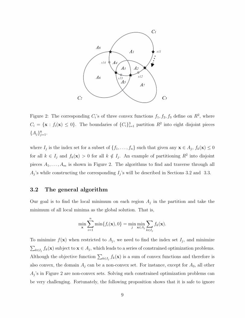
Figure 2: The corresponding Ci’s of three convex functions f1, f2, f3 define on R2, where
Ci = {x : fi(x) ≤ 0}. The boundaries of {Ci}3i=1 partition R2 into eight disjoint pieces
{Aj}8j=1.
where Ij is the index set for a subset of {f1, . . . , fn} such that given any x ∈ Aj, fk(x) ≤ 0
for all k ∈ Ij and fk(x) > 0 for all k /∈ Ij. An example of partitioning R2 into disjoint
pieces A1, . . . , Am is shown in Figure 2. The algorithms to find and traverse through all
Aj’s while constructing the corresponding Ij’s will be described in Sections 3.2 and 3.3.
3.2 The general algorithm
Our goal is to find the local minimum on each region Aj in the partition and take the
minimum of all local minima as the global solution. That is,
minx
n∑i=1
min{fi(x), 0} = minj
minx∈Aj
∑k∈Ij
fk(x).
To minimize f(x) when restricted to Aj, we need to find the index set Ij, and minimize∑k∈Ij fk(x) subject to x ∈ Aj, which leads to a series of constrained optimization problems.
Although the objective function∑
k∈Ij fk(x) is a sum of convex functions and therefore is
also convex, the domain Aj can be a non-convex set. For instance, except for A3, all other
Aj’s in Figure 2 are non-convex sets. Solving such constrained optimization problems can
be very challenging. Fortunately, the following proposition shows that it is safe to ignore
9
the constraint x ∈ Aj when minimizing∑
k∈Ij fk(x), and consequently, we only need to
solve a series of unconstrained convex optimization problems, which is much easier.
Proposition 3.2. Using the notations defined in Section 3.1, we have
minx
n∑i=1
min{fi(x), 0} = minj
minx
∑k∈Ij
fk(x)
Based on Proposition 3.2, a general framework for minimizing (6) is to enumerate all
the regions {Aj}mj=1 and solve a unconstrained convex optimization problem for each region.
See Supplementary Algorithm S1 for details.
3.3 Implementation in low-dimensional settings
The implementation of the general algorithm described above depends on both the class
of functions {fi}ni=1 and the dimension d. When d = 1, each Ci is an interval on the real
line and the boundary of Ci, ∂Ci, is composed of the two end-points of Ci, which are the
locations where fi crosses zero. Without loss of generality, assuming that the 2n end-points
of {Ci}ni=1 are all distinct, we can then order them sequentially along the real line which
partitions R into m = 2n+ 1 fragments {Aj}mj=1. We can then go through them one by one
sequentially and in the same time keep track of functions entering and leaving the set of
untruncated functions on each fragment Aj. The detailed procedure for finding the global
minimizer of f(x) in 1-D is described in Supplementary Algorithm S2.
When d = 2, each Ci is a convex region on R2, and its boundary ∂Ci is a curve. One
way to enumerate all the Aj’s is to travel along each ∂Ci, and record the intersection points
of ∂Ci and ∂Ck for k 6= i. We then use these intersection points to keep track of functions
entering and leaving the set of untruncated functions on each Aj. The detailed procedure
for finding the global minimizer of f(x) in 2-D is described in Supplementary Algorithm S3.
Using the notations in Section 3.1 and the example in Figure 2 as an illustration, we
start from an arbitrary point x11 on ∂C1. On one side we have the region A1, on which
there is only one untruncated function (I1 = {1}). On the other side we have A8, on which
every function is truncated (I8 = ∅). Traveling clockwise, we come across ∂C3. At this
point, we add f3, which gives the sets of untruncated functions on A2 (I2 = {1, 3}) and A7
(I7 = {3}). Similarly, we obtain I3 = {1, 2, 3} and I5 = {2, 3} when we come across ∂C2.
10

When we come acoss ∂C3 for the second time, we remove f3 from the set of untruncated
function and obtain I4 = {1, 2} and I6 = {2}. By repeating the process for all Ci’s, we
enumerate the set of untruncated functions on all Aj’s.
What remains to be supplied in the 1-D algorithm are methods to find the end-points of
any given Ci, and to minimize the sum of a subset of untruncated functions. Similarly, for
the 2-D algorithm we need ways to find the intersection points of any given ∂Ci and ∂Ck,
and to minimize the sum of a subset of untruncated functions. The implementation of these
steps depends on the class of functions that we are dealing with. For some function classes,
solutions for these steps are either straightforward, or already well-studied. For instance,
for quadratic functions, finding the end-points (in 1-D) or finding the intersections (in 2-D)
requires solving quadratic equations, for which closed-form solutions exist. Minimizing the
sum of a subset of quadratic functions can also be solved in closed-form. For convex shape
placement problem described in Section 2.2, published algorithms exist for these steps for
commonly encountered convex shapes such as circles or convex polygons (De Berg et al.,
2000). For more general convex functions (e.g., those described in Section 2.1 for GLMs),
iterative algorithms (e.g., gradient descent or the Newton-Raphson method) can be used
for these steps.
3.4 Extension to high-dimensional settings
In three or higher dimensions, our algorithm can be implemented by following the same idea
of tracking all the intersection points as in the 2-D case. Essentially, each boundary ∂Ci
is a d− 1 dimensional surface, and enumerating all the Aj’s can be achieved by traversing
through all the pieces on each ∂Ci that are formed by its intersections with all other ∂Ck’s,
which is in turn a d − 1 dimensional problem. For instance, when d = 3, we need to find
all the intersection curves of ∂Ci and ∂Ck (both of which are surfaces) for i 6= k, and
traverse along each intersection curve while keep tracking all other surfaces ∂Cj, j 6= i 6= k,
it crosses. Apparently, this algorithm becomes increasingly complicated and inefficient for
larger d, which renders it impractical.
Here, we propose a compromised but efficient extension of our proposed algorithm to
high-dimensional settings. The price we pay is to give up the global minimizer, which is
11

sensible choice as Proposition (3.1) has shown that the general problem is NP-Hard. In
particular, we propose to solve for an approximate solution using a cyclic coordinate descent
algorithm, where we optimize one parameter a time while keeping all other parameters
fixed, and cycle through all the parameters until converge. When restricting to only one
parameter, the objective function is simply a sum of truncated convex functions in 1D.
Therefore, we can use our 1-D algorithm to solve this subproblem in each iteration. This
algorithm is guaranteed to converge since the objective function is bounded below and
its value is descending after each iteration. See Supplementary Algorithm S4 for details.
We will evaluate the performance of this algorithm using both simulated and real data
experiments in Section 4.4.
3.5 Time complexity analysis
For time complexity analysis of our proposed algorithms, in low-dimensional settings, we
can regard the dimension d as a constant. That is, any univariate function of d can be
considered as O(1).
For the 1-D algorithm, finding the 2n end-points takes O(nS) time, where S is the
time for finding the two endpoints of a given function. Ordering the 2n end-points takes
O(n log n) time. Traversing through all the end-points takes O(nT ) time, where T is the
time for minimizing the sum of a subset of untruncated functions. Similarly, for the 2-D
algorithm, finding all the intersection points takes O(n2S) time, where S is the time for
finding all the intersection points of any two given functions. Sorting all the intersection
points along all the boundaries {∂Ci}ni=1 takes O(n2K log(nK)) time, where K is the max-
imum number of intersection points any two boundaries ∂Ci and ∂Cj can have. Traversing
through all the intersection points takes O(n2KT ) time.
First, we show that K = O(1) for a large class of truncated convex functions. That is,
given any two truncated convex functions in the class, the maximum number of intersection
points their boundaries can have is bounded by a constant.
Definition 3.3. For any positive integer k ∈ Z+, a class of curves C in R2 is said to be k-
intersecting if and only if for any two distinct curves in C, the number of their intersection
points is at most k.
12

Definition 3.4. A class of truncated functions in R2 is said to be k-intersecting if and
only if the set of their truncation boundaries is k-intersecting.
Example 3.5. The class of truncated quadratic functions in R2 with positive definite Hes-
sian matrices is k-intersecting with k = 4. This is easy to see given the facts that the
truncation boundary of a quadratic function in R2 with positive definite Hessian matrix is
an ellipse, and two distinct ellipses can have at most four intersection points.
In fact, according to Bezout’s theorem, the number of intersection points of two distinct
plane algebraic curves is at most equal to the product of the degrees of the corresponding
polynomials. Therefore, a class F of truncated bivariate polynomials is k2-intersecting if
for any function f ∈ F its untruncated version is a polynomial of degree at most k.
While S and T depend on the class of functions that we are dealing with, for some
function classes, we have S = O(1) and T = O(1). That is, they both take constant time.
Example 3.6. For quadratic functions with positive definite Hessian matrices, T = O(1).
This is easy to see given the following three facts:
1. Given n quadratic functions fi = 12xTAix + bTi x + ci, i = 1, . . . , n, their sum is∑
i fi(x) = 12xTAx + bTx + c, where A =
∑i Ai,b =
∑i bi, and c =
∑i ci, which is
also a quadratic function.
2. To update the sum of quadratic functions when adding a new function to the sum
or removing an existing function from the sum, we only need to update A,b and c,
which takes O(1) time (it is in fact O(d2) time but can be simplified as O(1) time
since we consider d as a constant in low-dimensional settings).
3. The minimizer of any quadratic function 12xTAx + bTx + c with positive definite
Hessian matrix is −A−1b, which takes O(1) time to compute (it is in fact O(d3) time
but can be simplified as O(1) time since we consider d as a constant in low-dimensional
settings).
Furthermore, S = O(1), since all the intersection points (up to four of them) of any two
given ellipses can be found using closed-form formulas (Richter-Gebert, 2011).
13

Putting Examples 3.5 and 3.6 together, we know that the running time of the 1-D
algorithm for sum of truncated quadratic functions with positive definite Hessian matrix
is O(n log n), and the running time of the 2-D Algorithm for sum of truncated quadratic
functions with positive definite Hessian matrix is O(n2 log n). The time complexity analysis
for other class of functions can be conducted similarly.
In high-dimensional settings, however, the running time of the general algorithm will
be at least O(nd log n), where d is the dimension. In another word, the running time grows
exponentially as the dimension increases, which is typical for NP-Hard problems. It is easy
to see that the running time of the cyclic coordinate descent algorithm is O(kdn log n),
where k is the number iterations to converge, and O(dn log n) is the time for each round of
d one-dimensional updates.
4 Experiments
4.1 Outlier detection in simple linear regression
We simulate data for outlier detection in simple linear regression as described in Section 2.1
and compare the performance of our proposed method with the Θ-IPOD algorithm (She
and Owen, 2012) and three other robust estimation methods: MM-estimator (Yohai, 1987),
least trimmed squares (LTS) (Rosseeuw and Leroy, 1987) and Gervini and Yohai (2002)
one-step procedure (denoted as GY). Our goal is to estimate the regression coefficients
and identify the outliers with σ assumed to be 1. In other words, we try to estimate
β and γ in (2). Given n observations and k outliers, let X = [1n, (x1, . . . ,xn)T ], β =
(β0, β1)T = (1, 2)T , and L be a parameter controlling the leverage of the outliers. When
L > 0, xi is drawn from uniform(L,L + 1) for i = 1, . . . , k, and from uniform(−15, 15)
for i = k + 1, . . . , n. γ = (γ1, . . . , γn)T represents deviations from the means, and each γi
is drawn from exponential(0.1) + 3 for i = 1, . . . , k, and γi = 0 for i = k + 1, . . . , n. Based
on a popular choice for√λ as 2.5σ (She and Owen, 2012; Wilcox, 2005; Maronna et al.,
2006), we set√λ as 2.5.
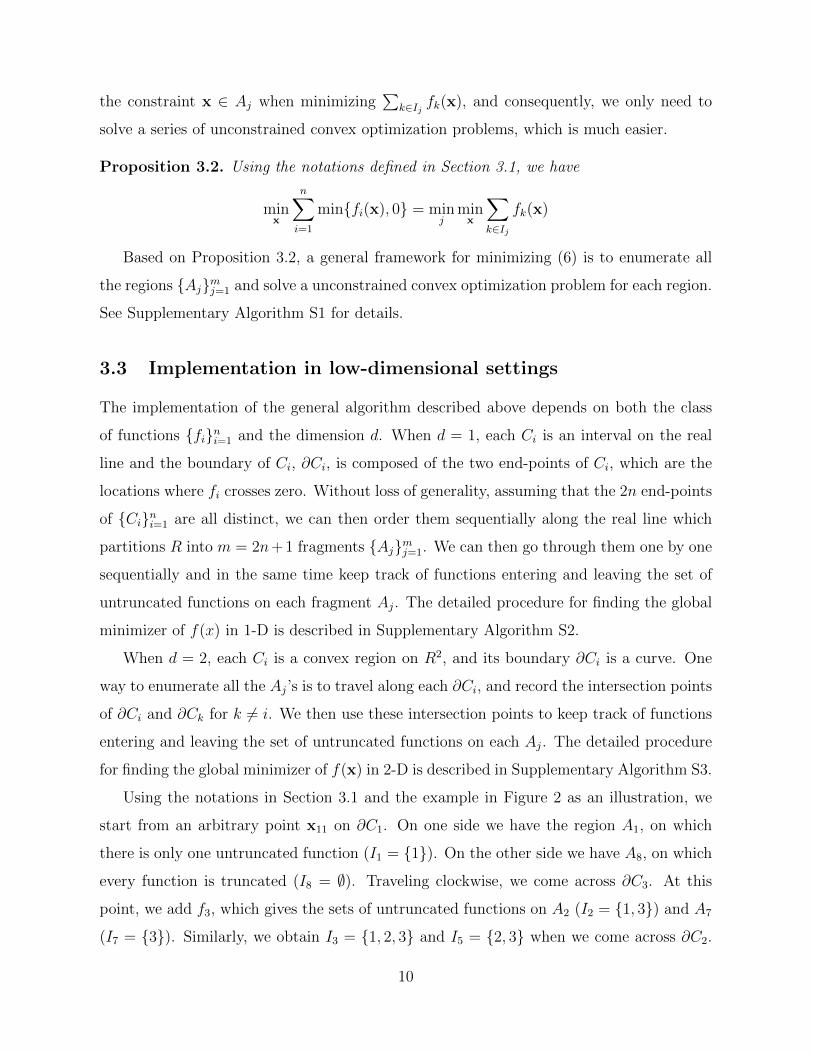
We simulate 100 independent data sets, each with 100 observations (i.e., n = 100).
The results are shown in Figure 3 and Supplementary Table S1. The performance of each
14

method is evaluated by the masking probability and the swamping probability under two
scenarios: (i) No L applied (denotes as L = 0), that is, xi is drawn from uniform(−15, 15)
for i = 1, . . . , n, and (ii) L = 20. Masking probability, as in She and Owen (2012), is defined
as the proportion of undetected true outliers among all outliers. Swamping probability, on
the other hand, is the fraction of normal observations recognized as outliers. We can see
that the proposed method outperforms others, especially when the number of outliers is
high.
4.2 Sum of truncated quadratic functions
We simulate sum of truncated quadratic functions with positive definite Hessian matrix
in R2 and compare the performance of the proposed algorithm with several other com-
peting algorithms including a global search algorithm (the DIRECT algorithm) (Jones
et al., 1993) and a branch-and-bound global optimization algorithm (StoGO) (Madsen and
Zertchaninov, 1998) both implemented in R package nloptr, a generalized simulating anneal-
ing algorithm (SA) implemented in R package GenSA (Xiang et al., 2013), a particle swarm
optimization algorithm (PSO) implemented in R package hydroPSO (Zambrano-Bigiarini
and Rojas, 2013), as well as the difference of convex functions (DC) algorithm (An and
Tao, 1997) which has been used to solve problems with truncated convex functions (Shen
et al., 2012; Chen et al., 2016). We implement the DC algorithm in R (see Supplementary
Section S1.4 for details).
Following (Hendrix et al., 2010), we compare the performance of all the algorithms in
terms of their effectiveness in finding the global minimum. We measure effectiveness by the
success rate, where a success for a given algorithm in a given run is defined as having the
estimated minimum no greater than any other algorithms by 10−5. This tolerance value
is allowed to accommodate numerical precision issues. We set a maximum number of 104
function evaluations, a maximum number of 104 iterations and a convergence tolerance
level of 10−8 for all competing algorithms whenever possible. See Supplementary Table S2
for details.
We randomly generate truncated quadratic functions in R2 with varying degrees of
complexity. Specifically, given a quadratic function with positive definite Hessian matrix
15
10 20 30 40 50 60
020
4060
8010
0 Leverage of outliers L = 0
Percent outliers (O%)
Per
cent
mas
king
(M
%)
● ● ● ●
●
●
● MMLTSGYIPODProposed
10 20 30 40 50 60
020
4060
8010
0 Leverage of outliers L = 0
Percent outliers (O%)
Per
cent
sw
ampi
ng (
S%
)
● ● ● ●
●
●● MMLTSGYIPODProposed
10 20 30 40 50 60
020
4060
8010
0 Leverage of outliers L = 20
Percent outliers (O%)P
erce
nt m
aski
ng (
M%
)
● ● ●
●
● ●
● MMLTSGYIPODProposed
10 20 30 40 50 60
020
4060
8010
0 Leverage of outliers L = 20
Percent outliers (O%)
Per
cent
sw
ampi
ng (
S%
)
● ● ●●
●
●
● MMLTSGYIPODProposed
Figure 3: Comparison of different methods for outlier detection in simple linear regression.
The figures show the mean percents of masking (top) and swamping (bottom) for different
leverages of outliers: L = 0 (left) and L = 20 (right) and differnt percents of outliers (O%)
for all the methods using 100 simulated replicates. The standard errors of the means are
shown as error bars.
16
0.0 0.2 0.4 0.6 0.8 1.0
0.0
0.2
0.4
0.6
0.8
1.0 C = 1
0.0 0.2 0.4 0.6 0.8 1.0
0.0
0.2
0.4
0.6
0.8
1.0 C = 5
0.0 0.2 0.4 0.6 0.8 1.0
0.0
0.2
0.4
0.6
0.8
1.0 C = 10
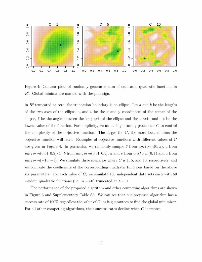
Figure 4: Contour plots of randomly generated sum of truncated quadratic functions in
R2. Global minima are marked with the plus sign.
in R2 truncated at zero, the truncation boundary is an ellipse. Let a and b be the lengths
of the two axes of the ellipse, u and v be the x and y coordinates of the center of the
ellipse, θ be the angle between the long axis of the ellipse and the x axis, and −z be the
lowest value of the function. For simplicity, we use a single tuning parameter C to control
the complexity of the objective function. The larger the C, the more local minima the
objective function will have. Examples of objective functions with different values of C
are given in Figure 4. In particular, we randomly sample θ from uniform(0, π), a from
uniform(0.01, 0.5)/C, b from uniform(0.01, 0.5), u and v from uniform(0, 1) and z from
uniform(−10,−1). We simulate three scenarios where C is 1, 5, and 10, respectively, and
we compute the coefficients of the corresponding quadratic functions based on the above
six parameters. For each value of C, we simulate 100 independent data sets each with 50
random quadratic functions (i.e., n = 50) truncated at λ = 0.
The performance of the proposed algorithm and other competing algorithms are shown
in Figure 5 and Supplementary Table S3. We can see that our proposed algorithm has a
success rate of 100% regardless the value of C, as it guarantees to find the global minimizer.
For all other competing algorithms, their success rates decline when C increases.
17

2 4 6 8 10
020
4060
8010
0
C
Per
cent
suc
cess
● ●
●
● DIRECTStoGOSAPSODCProposed
Figure 5: Comparison of different algorithms for minimizing the sum of 50 randomly gen-
erated truncated quardratic funstions in 2-D. The figure shows the mean success rates (in
percents) for all the methods using 100 simulated replicates for different complexities of
the functions (C). The standard errors of the means are shown as error bars.
4.3 Convex shape placement
Following Section 2.2, we randomly sample 30 points (i.e., n = 30) uniformly from the
[0, 1] × [0, 1] unit square, and use our proposed algorithm to find a location to place S
such that it covers the maximum number of points. To demonstrate the generality of our
proposed algorithm, we consider three shapes here: circle, square and hexagon. The results
are shown in Supplementary Figure S1.
18

4.4 Signal and image restoration
Following Section 2.3, we simulate 1-D signal with additive Gaussian noise, and compare the
performance of the proposed algorithm with several other algorithms including DIRECT,
StoGO, SA, PSO (See Section 4.2 for more details of these algorithms) and a recently
published iterative marginal optimization (IMO) algorithm (Portilla et al., 2015), which was
specifically designed for signal and image restoration. We implement the IMO algorithm
in R (see Supplementary Section S1.5 for details). The DC algorithm turns out to be
numerically equivalent to the IMO algorithm, but much slower. Therefore, we did not
included the DC algorithm in the comparison, and simply named the IMO algorithm as
IMO/DC.
The data are simulated by adding random Gaussian noise sampled i.i.d. from N(0, 1)
to an underlying true signal. Each data set contains 100 data points equally spaced on
the interval [0, 1]. The true signal is design to be piece-wise smooth with different pieces
being constant, linear, quadratic or sine waves (see Figure 6). All the algorithms are used
to restore the signal by minimizing the following objective function,
y = arg miny
d∑i=1
(yi − yi)2 + wd−1∑i=1
min{(yi − yi+1)2, λ},
where d = 100, yi and yi, i = 1, . . . , d, are the observed and restored values at data point
i, respectively. That is, we are solving the sum of 199 truncated quadratic functions (99
of them are truncated at λ, and the remaining 100 of them are truncated at infinity) in a
100-dimensional parameter space. The tuning parameters are empirically set as w = 4 and
λ = 9, respectively.
We measure the performance of these algorithms using four different metrics:
1. Success rate, which is defined in Section 4.2. Note a success here only means that a
given algorithm has found the best solution among all algorithms, which may or may
not be the global minimizer.
2. Relative loss, which is defined as |f(y) − f(y∗)|/|f(y∗)|, where y and y∗ are the
solution found by a given algorithm and the best solution found by all algorithms,
respectively.
19

0.0 0.2 0.4 0.6 0.8 1.0
−5
05
10
x
y
0.0 0.2 0.4 0.6 0.8 1.0
−5
05
10
x
y
Figure 6: Simulated random signal (left) and restored signal (right) are shown in solid
lines. The underlying true signal are shown in dashed lines.
3. Root mean square error (RMSE), which is defined as√d−1
∑di=1(yi − yi)2, where y
and y are the solution found by a given algorithm and the underlying true signal,
respectively.
4. Running time, measured in seconds.
The performance of the proposed algorithm and other competing algorithms are summa-
rized in Table 1. In general, the proposed algorithm outperforms all other methods in
terms of success rate, relative loss and RMSE. It is also significantly faster than all other
algorithms.
Finally, we apply the proposed algorithm for image restoration. Both synthetic and
real images are used for this experiment (see Figure 7 and Supplementary Figure S2). All
images are resized to 256 × 256, converted to gray scale and normalized to have pixel
intensity levels in [0, 1]. Independent Gaussian noise sampled from N(µ = 0, σ2 = 0.01) is
added to each pixel, and the proposed algorithm is used to restore the original image via
minimizing the following objective function,
z = arg minz
∑i∈I
(zi − zi)2 + w∑
i,j∈I,i∈D(j)
min{(zi − zj)2, λ},
20

Table 1: Comparison of different algorithms for signal restoration. The table shows the
mean success rates (in percents), relative losses, root mean square errors (RMSE), as well
as running times (in seconds) for all the methods using 100 simulated replicates. The
standard errors of the means are given in parentheses.
DIRECT StoGO SA PSO IMO/DC Proposed
Success rate 0.0 (0.0) 8.0 (2.7) 52.0 (5.0) 0.0 (0.0) 28.0 (4.5) 84.0 (3.7)
Relative loss 0.08 (0.00) 0.05 (0.02) 0.04 (0.01) 0.17 (0.01) 0.10 (0.01) 0.01 (0.00)
RMSE 0.66 (0.01) 0.56 (0.01) 0.59 (0.01) 0.63 (0.01) 0.56 (0.01) 0.55 (0.01)
Time 0.40 (0.00) 61.29 (0.27) 0.31 (0.00) 12.39 (0.13) 1.50 (0.07) 0.04 (0.00)
where zi and zi, i ∈ I, are the observed and restored intensity values at pixel i, respectively,
i ∈ D(j) means that pixels i and j are neighbors of each other, and the tuning parameters
are empirically set as w = 2 and λ = 0.02, respectively. From Figure 7 and Supplementary
Figure S2, we see that compared with Gaussian smoothing, the proposed algorithm can
restore the smoothness in the image while maintaining the sharp edges. Even though this
problem has a dimension of d = 256×256 = 65, 536 and the number of truncated quadratic
functions is n = 256 × 256 + 2 × 256 × 255 = 196, 096, it only takes about 10 seconds for
our algorithm to converge.
5 Discussion
We know that summing convex functions together still gives us a convex function. Although
simply truncating the function at a given level does not seem to add much complexity to
a convex function, the sum of truncated convex functions is not in the same class as its
summands, which makes it very powerful and flexible in modeling various kinds of problems,
as several examples given in Section 2. Figure 4 further demonstrates the diverse landscape
that can be achieved by a sum of truncated quadratic functions. This flexibility is supported
by Proposition 3.1, which implies that any problem in the class of NP can be reduced to
the minimization of a sum of truncated convex functions. A potential future work is to
approximate a given non-convex function by a sum of truncated quadratic functions and
then use our proposed algorithm to minimize it.
21

Figure 7: Restoration of synthetic and real images. For each row, from left to right: original
image, image with Gaussian noise added, image restored using Gaussian smoothing with a
5× 5 kernel and image restored using proposed algorithm.
In the cyclic coordinate descent algorithm, instead of performing a univariate update in
each round, we can also perform a bivariate update in each round using the 2-D algorithm
(i.e., using a block coordinate descent algorithm), which may help increase the chance of
finding the global minimizer, at the cost of more intensive computation.
Besides the applications described in this paper, minimizing sum of truncated con-
vex functions also has many other applications, such as detecting differential gene ex-
pression (Jiang and Zhan, 2016) (See Supplementary Section S1.1) and personalized dose
finding (Chen et al., 2016). This paper demonstrates that the proposed algorithm can be
quite efficient when the truncation boundaries of the class of convex functions are simple
shapes such as ellipse and convex polygon, which cover the cases of truncated quadratic
functions and truncated `1 penalty (TLP (Shen et al., 2012)). Although these functions
are seemingly limited, their applications are vastly abundant, and we have shown only a
few selected examples in this paper. In our future work, we will investigate the application
of our proposed algorithm to other classes of convex functions.
22

R programs for reproducing the results in this paper are available at http://www-personal.
umich.edu/~jianghui/stcf/.
Supplementary materials
Supplementary texts, algorithms, proofs, figures and tables. (supplementary.pdf)
Acknowledgements
We thank the two anonymous reviewers and the associate editor for their suggestions on
the image restoration application and the extension to high-dimension settings. Their
comments and suggestions have helped us improve the quality of this paper substantially.
References
Agarwal, A. and H. Daume III (2011). Generative kernels for exponential families. In
AISTATS, pp. 85–92.
An, L. T. H. and P. D. Tao (1997). Solving a class of linearly constrained indefinite
quadratic problems by dc algorithms. Journal of global optimization 11 (3), 253–285.
Barequet, G., M. Dickerson, and P. Pau (1997). Translating a convex polygon to contain
a maximum number of points. Computational Geometry 8 (4), 167–179.
Boyd, S. and L. Vandenberghe (2004). Convex optimization. Cambridge university press.
Candes, E. J. and T. Tao (2010). The power of convex relaxation: Near-optimal matrix
completion. Information Theory, IEEE Transactions on 56 (5), 2053–2080.
Chazelle, B. M. and D.-T. Lee (1986). On a circle placement problem. Computing 36 (1-2),
1–16.
Chen, G., D. Zeng, and M. R. Kosorok (2016). Personalized dose finding using outcome
weighted learning. Journal of the American Statistical Association 111 (516), 1509–1521.
23
Cook, S. A. (1971). The complexity of theorem-proving procedures. In Proceedings of the
third annual ACM symposium on Theory of computing, pp. 151–158. ACM.
De Berg, M., M. Van Kreveld, M. Overmars, and O. C. Schwarzkopf (2000). Computational
geometry. In Computational geometry, pp. 1–17. Springer.
Fan, J. and R. Li (2001). Variable selection via nonconcave penalized likelihood and its
oracle properties. Journal of the American statistical Association 96 (456), 1348–1360.
Gannaz, I. (2007). Robust estimation and wavelet thresholding in partially linear models.
Statistics and Computing 17 (4), 293–310.
Georgogiannis, A. (2016). Robust k-means: a theoretical revisit. In Advances in Neural
Information Processing Systems, pp. 2883–2891.
Gervini, D. and V. J. Yohai (2002). A class of robust and fully efficient regression estimators.
Annals of Statistics , 583–616.
Hendrix, E. M., G. Boglarka, et al. (2010). Introduction to nonlinear and global optimiza-
tion. Springer New York.
Jiang, H. and J. Salzman (2015). A penalized likelihood approach for robust estimation of
isoform expression. Statistics and Its Interface 8, 437–445.
Jiang, H. and T. Zhan (2016). Unit-free and robust detection of differential expression from
rna-seq data. arXiv preprint arXiv:1405.4538v3 .
Jones, D. R., C. D. Perttunen, and B. E. Stuckman (1993). Lipschitzian optimization
without the lipschitz constant. Journal of Optimization Theory and Applications 79 (1),
157–181.
Karp, R. M. (1972). Reducibility among combinatorial problems. Springer.
Katayama, S. and H. Fujisawa (2015). Sparse and robust linear regression: An optimization
algorithm and its statistical properties. arXiv preprint arXiv:1505.05257 .
Lee, Y., S. N. MacEachern, and Y. Jung (2012). Regularization of case-specific parameters
for robustness and efficiency. Statistical Science, 350–372.
24

Madsen, K. and S. Zertchaninov (1998). A new branch-and-bound method for global op-
timization. IMM, Department of Mathematical Modelling, Technical Universityof Den-
mark.
Maronna, R., D. Martin, and V. Yohai (2006). Robust statistics. John Wiley & Sons,
Chichester. ISBN.
McCann, L. and R. E. Welsch (2007). Robust variable selection using least angle regression
and elemental set sampling. Computational Statistics & Data Analysis 52 (1), 249–257.
Mehrez, A. and A. Stulman (1982). The maximal covering location problem with facility
placement on the entire plane. Journal of Regional Science 22 (3), 361–365.
Michael, R. G. and S. J. David (1979). Computers and intractability: a guide to the theory
of np-completeness. WH Free. Co., San Fr .
Nasrabadi, N. M., T. D. Tran, and N. Nguyen (2011). Robust lasso with missing and
grossly corrupted observations. In Advances in Neural Information Processing Systems,
pp. 1881–1889.
Nikolova, M. (2000). Thresholding implied by truncated quadratic regularization. IEEE
Transactions on Signal Processing 48 (12), 3437–3450.
Nikolova, M. (2011). Energy minimization methods. In Handbook of mathematical methods
in imaging, pp. 139–185. Springer.
Nikolova, M., M. K. Ng, and C.-P. Tam (2010). Fast nonconvex nonsmooth minimiza-
tion methods for image restoration and reconstruction. IEEE Transactions on Image
Processing 19 (12), 3073–3088.
Portilla, J., A. Tristan-Vega, and I. W. Selesnick (2015). Efficient and robust image restora-
tion using multiple-feature l2-relaxed sparse analysis priors. IEEE Transactions on Image
Processing 24 (12), 5046–5059.
Richter-Gebert, J. (2011). Perspectives on projective geometry: A guided tour through real
and complex geometry. Springer Science & Business Media.
25

Rosseeuw, P. J. and A. M. Leroy (1987). Robust regression and outlier detection. Wiley
Series in Probability and Mathematical Statistics, New York: Wiley 1.
She, Y. and A. B. Owen (2012). Outlier detection using nonconvex penalized regression.
Journal of the American Statistical Association.
Shen, X., W. Pan, and Y. Zhu (2012). Likelihood-based selection and sharp parameter
estimation. Journal of the American Statistical Association 107 (497), 223–232.
Tibshirani, J. and C. D. Manning (2014). Robust logistic regression using shift parameters.
In ACL (2), pp. 124–129.
Wilcox, R. R. (2005). Robust testing procedures. Encyclopedia of Statistics in Behavioral
Science.
Witten, D. M. (2013). Penalized unsupervised learning with outliers. Statistics and its
Interface 6 (2), 211.
Xiang, Y., S. Gubian, B. Suomela, and J. Hoeng (2013). Generalized simulated annealing
for global optimization: the gensa package. R Journal 5 (1), 13–28.
Yohai, V. J. (1987). High breakdown-point and high efficiency robust estimates for regres-
sion. The Annals of Statistics , 642–656.
Zambrano-Bigiarini, M. and R. Rojas (2013). A model-independent particle swarm opti-
misation software for model calibration. Environmental Modelling & Software 43, 5–25.
Zhigljavsky, A. and A. Zilinskas (2007). Stochastic global optimization, Volume 9. Springer
Science & Business Media.
26
Supplementary Materials for “Minimizing Sum of Truncated
Convex Functions and Its Applications”
S1 Supplementary texts
S1.1 Application on detecting differential gene expression with
`0-penalized models
The idea of using the `0 penalty for variable selection can also be applied to the detection
of differentially expressed genes from RNA sequencing data. The problem is discussed
in detail in Jiang and Zhan (2016), and we briefly summarize the approach here. Given
S experimental groups each with ns biological samples, we would like to compare the
expression levels of m genes measured in the samples. Let µsi be the mean expression
level of gene i (on the log-scale) in group s, dsj be the scaling factor (e.g., sequencing
depth or library size on the log-scale) for sample j in group s, and σ2i be the variance of
expression level of gene i (on the log-scale). Assuming a linear model on the observed data
xsij ∼ N(µsi + dsj, σ2i ), the problem is to identify genes that are differentially expressed
across the groups. To do so, assuming {σi}mi=1 are known, reparametrizing µsi as µi =
µ1i, γsi = µsi − µ1i, s = 1, . . . , S, the `0-penalized negative log-likelihood function of the
model is
f(µ, γ, d) =m∑i=1
1
2σ2i
S∑s=1
ns∑j=1
(xsij − µi − γsi − dsj)2 +m∑i=1
αi1(S∑s=1
|γsi| > 0) (S1)
27
Where {αi}mi=1 are tuning parameters. It is shown in Jiang and Zhan (2016) that (S1) can
be solved as follows
d′sj = (∑m
i=1(xsij − xsi1)/σ2i )/(
∑mi=1 1/σ2
i ), s = 1, . . . , S
µ′si = (1/ns)∑ns
j=1(xsij − d′sj), s = 1, . . . , S
d1 = 0
d2, . . . , dS = arg mind2,...,dS
m∑i=1
min (g(d2, . . . , dS), αi)
where g(d2, . . . , dS) =1
2σ2i
S∑s=1
ns(µ′si − ds)2 −
1
n
[S∑s=1
(ns(µ′si − ds))
]2dsj = ds + d′sj, s = 1, . . . , S
γsi =
0 if g(d2, . . . , dS) < αi
µ′si − µ′1i − ds otherswise
µi =
(1/n)∑S
s=1 ns(µ′si − ds) if g(d2, . . . , dS) < αi
µ′1i otherwise
where the only computationally intensive step is to minimize a sum of truncated quadratic
functions in d2, . . . , dS
d2, . . . , dS = arg mind2,...,dS
m∑i=1
min{g(d2, . . . , dS), αi}.
Methods for choosing {αi}mi=1 and for estimating {σ2i }mi=1, as well as experiments on simu-
lated and real data, are given in Jiang and Zhan (2016).
28

S1.2 Algorithms described in Section 3
Algorithm S1 A general algorithm for minimizing (6).
procedure algorithm.general(f1, . . . , fn)
for i = 1 : n do
Find region Ci such that fi(x) ≤ 0 on Ci.
end for
Find all the pieces {Aj}mj=1 in the partition of Rd formed by {Ci}ni=1.
s← 0.
for j = 1 : m do
Find the set of functions {fk}k∈Ij that are not truncated on Aj.
s← min{s,minx
∑k∈Ij
fk(x)}.
end for
return s.
end procedure
29

Algorithm S2 An algorithm for minimizing (6) in 1-D.
procedure algorithm.1d(f1, . . . , fn)
for i = 1 : n do
Find the interval Ci = [li, ri] ⊂ R such that fi(x) ≤ 0 on Ci.
end for
Order all the 2n end-points of {Ci}ni=1 along the real line as p1 < · · · < p2n.
s← 0, I ← ∅.
for j = 1 : 2n do
if pj is the left end-point of an interval Ck then
Add k to set I.
else if pj is the right end-point of an interval Ck then
Remove k from set I.
end if
s← min{s,minx
∑k∈I
fk(x)}.
end for
return s.
end procedure
30

Algorithm S3 An algorithm for minimizing (6) in 2-D.
procedure algorithm.2d(f1, . . . , fn)
for i = 1 : n do
Find Ci ⊂ R2 such that fi(x) ≤ 0 on Ci.
Find ∂Ci, the boundary Ci.
end for
s← 0.
for i = 1 : n do
Find all the intersection points of ∂Ci and ∂Ck, k 6= i.
Sort all the intersection points along ∂Ci clockwise as p1, . . . ,pni.
Find a point p between p1 and pnion ∂Ci.
I ← {k : p ∈ Ck}, J ← I \ {i}.
for j = 1 : ni do
if pj is the intersection point of ∂Ci and ∂Ck and k ∈ I then
Remove k from sets I and J .
else if pj is the intersection point of ∂Ci and ∂Ck and k 6∈ I then
Add k to sets I and J .
end if
s← min{s,minx
∑k∈I
fk(x),minx
∑k∈J
fk(x)}.
end for
end for
return s.
end procedure
31

Algorithm S4 A cyclic coordinate descent algorithm for minimizing (6) in high-
dimensional settings.
procedure algorithm.high-d(f1, . . . , fn)
Initialize x as x0.
while true do
for j = 1 : d do
Fix all xk, k 6= j, minimize the objective function as a univariate function of
xj using Algorithm S2.
end for
if the change in x since the last iteration is less than a given tolerance level then
return x.
end if
end while
end procedure
S1.3 The Θ-IPOD algorithm for robust linear regression
Algorithm S5 The Θ-IPOD algorithm for robust linear regression, adapted from Algo-
rithm 2 in She and Owen (2012).
procedure Θ-IPOD(X ∈ Rn×p,y ∈ Rn,λ > 0 ∈ Rn,γ(0) ∈ Rp, and threshold operator
Θ(·; ·) which is taken as the hard-threshold operator Θh(·; ·) in our paper)
γ ← γ(0),H← X(XTX)−1XT , r← y −Hy.
while true do
γ ← Θh(Hγ + r;√λ).
if the change in γ since the last iteration is less than a given tolerance level then
return γ ← γ and β ← (XTX)−1XT (y − γ).
end if
end while
end procedure
32
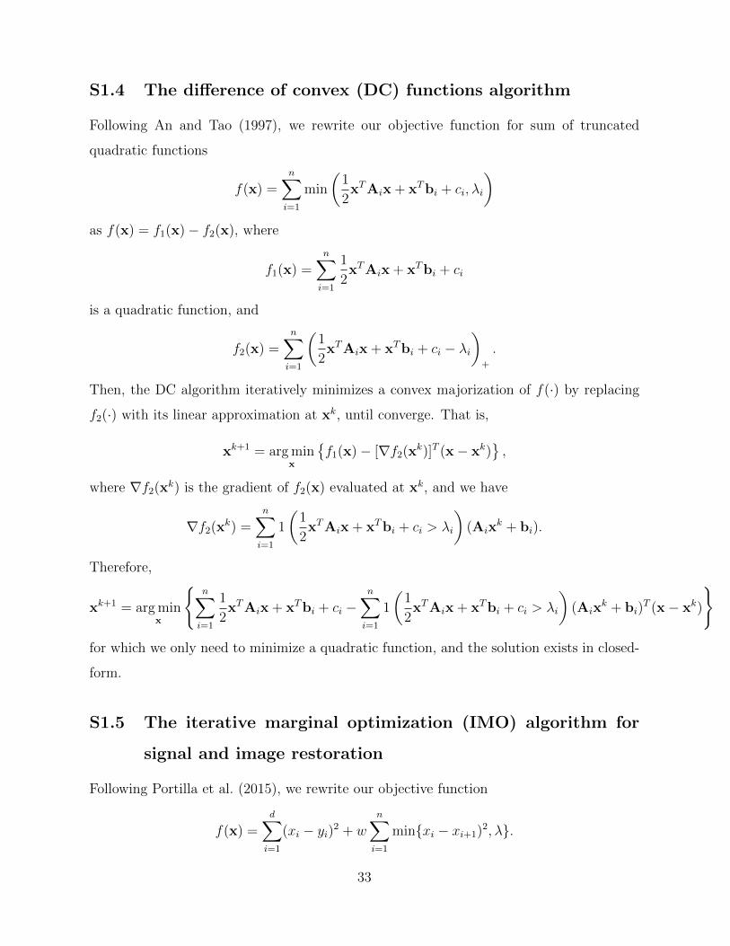
S1.4 The difference of convex (DC) functions algorithm
Following An and Tao (1997), we rewrite our objective function for sum of truncated
quadratic functions
f(x) =n∑i=1
min
(1
2xTAix + xTbi + ci, λi
)as f(x) = f1(x)− f2(x), where
f1(x) =n∑i=1
1
2xTAix + xTbi + ci
is a quadratic function, and
f2(x) =n∑i=1
(1
2xTAix + xTbi + ci − λi
)+
.
Then, the DC algorithm iteratively minimizes a convex majorization of f(·) by replacing
f2(·) with its linear approximation at xk, until converge. That is,
xk+1 = arg minx
{f1(x)− [∇f2(xk)]T (x− xk)
},
where ∇f2(xk) is the gradient of f2(x) evaluated at xk, and we have
∇f2(xk) =n∑i=1
1
(1
2xTAix + xTbi + ci > λi
)(Aix
k + bi).
Therefore,
xk+1 = arg minx
{n∑i=1
1
2xTAix + xTbi + ci −
n∑i=1
1
(1
2xTAix + xTbi + ci > λi
)(Aix
k + bi)T (x− xk)
}for which we only need to minimize a quadratic function, and the solution exists in closed-
form.
S1.5 The iterative marginal optimization (IMO) algorithm for
signal and image restoration
Following Portilla et al. (2015), we rewrite our objective function
f(x) =d∑i=1
(xi − yi)2 + wn∑i=1
min{xi − xi+1)2, λ}.
33

as
f(x) = ||Hx− y||2 + w
n∑i=1
min{(φTi x)2, λ},
where n = d − 1,H = In is an identity matrix, Φ = (φ1, . . . ,φn)T ∈ Rn×d with φi,i =
−1, φi,i+1 = 1 and otherwise φi,j = 0 for all i and j. We then minimize f(x) using the
following iterative algorithm proposed in Portilla et al. (2015), where Θh(·; ·) is the hard-
threshold operator.
Algorithm S6 The iterative marginal optimization (IMO) algorithm for signal and image
restoration, Adapted from Algorithm 1 in Portilla et al. (2015).
procedure Threshold(y ∈ Rd,Φ ∈ Rn×d,λ > 0 ∈ Rn)
x← y.
while true do
b← Φx.
a← Θh(b;√λ).
z← wΦTa.
x← (HTH + wΦTΦ)−1(HTy + z).
if the change in x since the last iteration is less than a given tolerance level then
return x.
end if
end while
end procedure
S2 Proofs
Proof of Proposition 2.1.
To minimize (3),
f(β,γ) =n∑i=1
(yi − xTi β − γi)2 + λ
n∑i=1
1(γi 6= 0),
notice that the minimization with respect to γ can be performed componentwise. For each
34
γi, if γi = 0, we have
f(β, γ1, . . . , γi = 0, . . . , γn) =∑j 6=i
{(yj − xTi β − γj)2 + λ1(γj 6= 0)
}+ (yi − xTi β)2. (S2)
On the other hand, if γi 6= 0, we have
f(β, γ1, . . . , γi 6= 0, . . . , γn) =∑j 6=i
{(yj − xTi β − γj)2 + λ1(γj 6= 0)
}+ (yi − xTi β − γi)2 + λ,
which is minimized at γi = yi − xTi β, that is,
f(β, γ1, . . . , γi = yi − xTi β, . . . , γn) =∑j 6=i
{(yj − xTi β − γj)2 + λ1(γj 6= 0)
}+ λ. (S3)
Comparing (S2) with (S3), it is easy to see that we should choose γi = 0 if (yi−xTi β)2 < λ
and γi = yi − xTi β othersise. Plugging the value of γi into (3), we have
f(β,γ) =n∑i=1
[(yi − xTi β)21{(yi − xTi β)2 < λ}+ λ1{(yi − xTi β)2 ≥ λ}
]=
n∑i=1
min{(yi−xTi β)2, λ}
which is the objective function g(β) in Proposition 2.1.
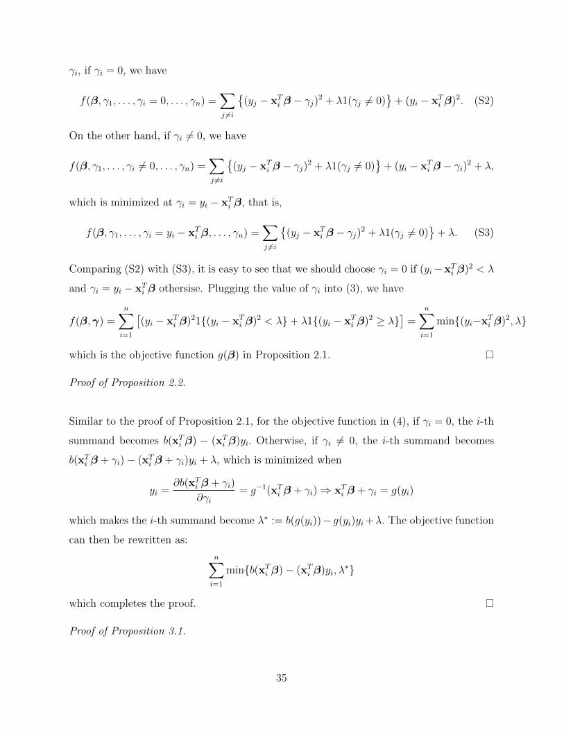
Proof of Proposition 2.2.
Similar to the proof of Proposition 2.1, for the objective function in (4), if γi = 0, the i-th
summand becomes b(xTi β) − (xTi β)yi. Otherwise, if γi 6= 0, the i-th summand becomes
b(xTi β + γi)− (xTi β + γi)yi + λ, which is minimized when
yi =∂b(xTi β + γi)
∂γi= g−1(xTi β + γi)⇒ xTi β + γi = g(yi)
which makes the i-th summand become λ∗ := b(g(yi))− g(yi)yi +λ. The objective function
can then be rewritten as:
n∑i=1
min{b(xTi β)− (xTi β)yi, λ∗}
which completes the proof.
Proof of Proposition 3.1.
35

Let b1, . . . , bn be n Boolean variables, i.e., each bk only takes one of two possible values:
TRUE or FALSE. For a 3-SAT problem P , suppose its formula is
f(b1, . . . , bn) = c1 ∧ · · · ∧ cm,
where ∧ is the logical OR operator, and {ci}mi=1 are the clauses1 of P with
ci = (li1 ∨ li2 ∨ li3),
where ∨ is the logical AND operator, and {lij}mi=1, j ∈ {1, 2, 3}, are literals of P . Each
literal lij is either a variable bk for which lij is called a positive literal, or the negation
of a variable ¬bk for which lij is called a negative literal. Without loss of generality,
suppose that each clause consists of exactly three literals, and that the three literals in
each clause correspond to three distinct variables. The 3-SAT problem P concerns about
the satisfiability of f(b1, . . . , bn), i.e., whether there exists a possible assignment of values
of b1, . . . , bn such that f(b1, . . . , bn) = TRUE.
We reduce the 3-SAT problem P to the minimization of a sum of truncated convex
functions g(x) : Rn → R as follows. Let x = (x1, . . . , xn) ∈ Rn with each xk corresponds
to a bk such that bk = TRUE if and only if xk > 0. For each clause ci = (li1 ∨ li2 ∨ li3) of
P , define a sum of seven truncated convex functions
gi(x) =7∑t=1
min(git(x), 1)
where
git(x) =
0 if x ∈ Sit1 ∩ Sit2 ∩ Sit3∞ otherwise
where Sitj is one of the two half-spaces defined by xk > 0 and xk ≤ 0, respectively, where
xk is the variable corresponding to lij, that is, lij = bk or lij = ¬bk. We choose Sitj as the
half-space defined by xk > 0 if and only if (b(j, t)− 12) has the same sign as lij, where b(j, t)
is the j-th digit (from left to right) of t when t ∈ {1, . . . , 7} is represented as three binary
digits. For instance, for a clause ci = (b1 ∨ ¬b2 ∨ b3), we have
gi1(x) =
0 if x1 ≤ 0, x2 > 0, x3 > 0
∞ otherwise
1A clause is a disjunction of literals or a single literal. In a 3-SAT problem each clause has exactly three
literals.
36

and
gi7(x) =
0 if x1 > 0, x2 ≤ 0, x3 > 0
∞ otherwise
Since all the half-spaces, as well as their intersections, are convex sets, all the git(x)’s are
convex functions. Furthermore, since the regions in which git(x) = 0, t ∈ {1, . . . , 7}, are
disjoint, it is easy to verify that gi(x) can only take one of two possible values
gi(x) =
6 if ci is satisfied by the assigned values of b1, . . . , bn
7 otherwise
where we choose bk = TRUE if and only if xk > 0. The reduction is then completed by
noticing that the 3-SAT problem P is satisfiable if and only if the minimum value of the
function g(x) =∑m
i=1 gi(x) is 6m, and that it is easy to see that the reduction can be done
in polynomial time.
Proof of Proposition 3.2.
On one hand, we have
minx
n∑i=1
min{fi(x), 0} = minj
minx∈Aj
∑k∈Ij
fk(x) ≥ minj
minx
∑k∈Ij
fk(x), (S4)
On the other hand, we have
minj
minx
∑k∈Ij
fk(x) ≥ minj
minx
∑k∈Ij
min{fk(x), 0}
≥ minj
minx
n∑i=1
min{fi(x), 0}
= minx
n∑i=1
min{fi(x), 0}
(S5)
Putting (S4) and (S5) together, we have
minx
n∑i=1
min{fi(x), 0} = minj
minx
∑k∈Ij
fk(x).
37

S3 Supplementary figures and tables
●
●
●
●
●
●
●
●
●
●
●
●
●
●
●
●
●
●
●
●
●
●
●
●
●
●●
●
●
●
0.0 0.2 0.4 0.6 0.8 1.0
0.0
0.2
0.4
0.6
0.8
1.0
●
●
●●●
●
●
●
●
●
●
●
●
●
●
●
●●
●
●
●
●
●
●
●
●●
●
●
●
0.0 0.2 0.4 0.6 0.8 1.00.
00.
20.
40.
60.
81.
0
●
●
●
●
●
●
●
●
●
●
●
●
●
●
●
●
●
●
●
●
●
●
●
●
●
●
●
●
●
●
0.0 0.2 0.4 0.6 0.8 1.0
0.0
0.2
0.4
0.6
0.8
1.0
Figure S1: Placement of different convex shapes to cover the maximum number of points
uniformly sampled from the unit square.
Figure S2: Restoration of images. For each row, from left to right: original image, image
with Gaussian noise added, image restored using Gaussian smoothing with a 5 × 5 kernel
and image restored using proposed algorithm.
38
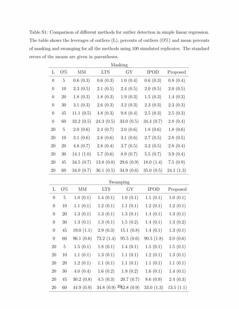
Table S1: Comparison of different methods for outlier detection in simple linear regression.
The table shows the leverages of outliers (L), percents of outliers (O%) and mean percents
of masking and swamping for all the methods using 100 simulated replicates. The standard
errors of the means are given in parentheses.
Masking
L O% MM LTS GY IPOD Proposed
0 5 0.6 (0.3) 0.6 (0.3) 1.0 (0.4) 0.6 (0.3) 0.8 (0.4)
0 10 2.3 (0.5) 2.1 (0.5) 2.4 (0.5) 2.0 (0.5) 2.0 (0.5)
0 20 1.8 (0.3) 1.8 (0.3) 1.9 (0.3) 1.5 (0.3) 1.4 (0.3)
0 30 3.1 (0.3) 2.6 (0.3) 3.2 (0.3) 2.3 (0.3) 2.3 (0.3)
0 45 11.1 (0.5) 4.8 (0.3) 9.8 (0.4) 2.5 (0.3) 2.5 (0.3)
0 60 33.2 (0.5) 24.3 (0.5) 33.0 (0.5) 34.4 (0.7) 2.8 (0.4)
20 5 2.0 (0.6) 2.4 (0.7) 2.0 (0.6) 1.8 (0.6) 1.8 (0.6)
20 10 3.1 (0.6) 2.8 (0.6) 3.1 (0.6) 2.7 (0.5) 2.8 (0.5)
20 20 4.8 (0.7) 2.8 (0.4) 3.7 (0.5) 3.2 (0.5) 2.8 (0.4)
20 30 14.1 (1.0) 5.7 (0.6) 8.9 (0.7) 5.5 (0.7) 3.9 (0.4)
20 45 34.5 (0.7) 13.8 (0.8) 29.6 (0.9) 18.0 (1.4) 7.5 (0.9)
20 60 34.0 (0.7) 36.1 (0.5) 34.9 (0.6) 35.0 (0.5) 24.1 (1.3)
Swamping
L O% MM LTS GY IPOD Proposed
0 5 1.0 (0.1) 1.4 (0.1) 1.0 (0.1) 1.1 (0.1) 1.0 (0.1)
0 10 1.1 (0.1) 1.2 (0.1) 1.1 (0.1) 1.2 (0.1) 1.2 (0.1)
0 20 1.3 (0.1) 1.3 (0.1) 1.3 (0.1) 1.4 (0.1) 1.3 (0.1)
0 30 1.3 (0.1) 1.3 (0.1) 1.5 (0.2) 1.4 (0.1) 1.3 (0.2)
0 45 19.0 (1.1) 2.9 (0.3) 15.1 (0.8) 1.4 (0.1) 1.3 (0.1)
0 60 96.1 (0.6) 73.2 (1.4) 95.5 (0.6) 90.5 (1.8) 2.0 (0.6)
20 5 1.5 (0.1) 1.8 (0.1) 1.4 (0.1) 1.5 (0.1) 1.5 (0.1)
20 10 1.1 (0.1) 1.3 (0.1) 1.1 (0.1) 1.2 (0.1) 1.3 (0.1)
20 20 1.2 (0.1) 1.1 (0.1) 1.1 (0.1) 1.1 (0.1) 1.1 (0.1)
20 30 4.0 (0.4) 1.6 (0.2) 1.9 (0.2) 1.6 (0.1) 1.4 (0.1)
20 45 30.2 (0.8) 4.5 (0.3) 20.7 (0.7) 8.6 (0.9) 2.4 (0.3)
20 60 44.9 (0.9) 34.8 (0.9) 42.8 (0.9) 33.0 (1.3) 13.5 (1.1)39
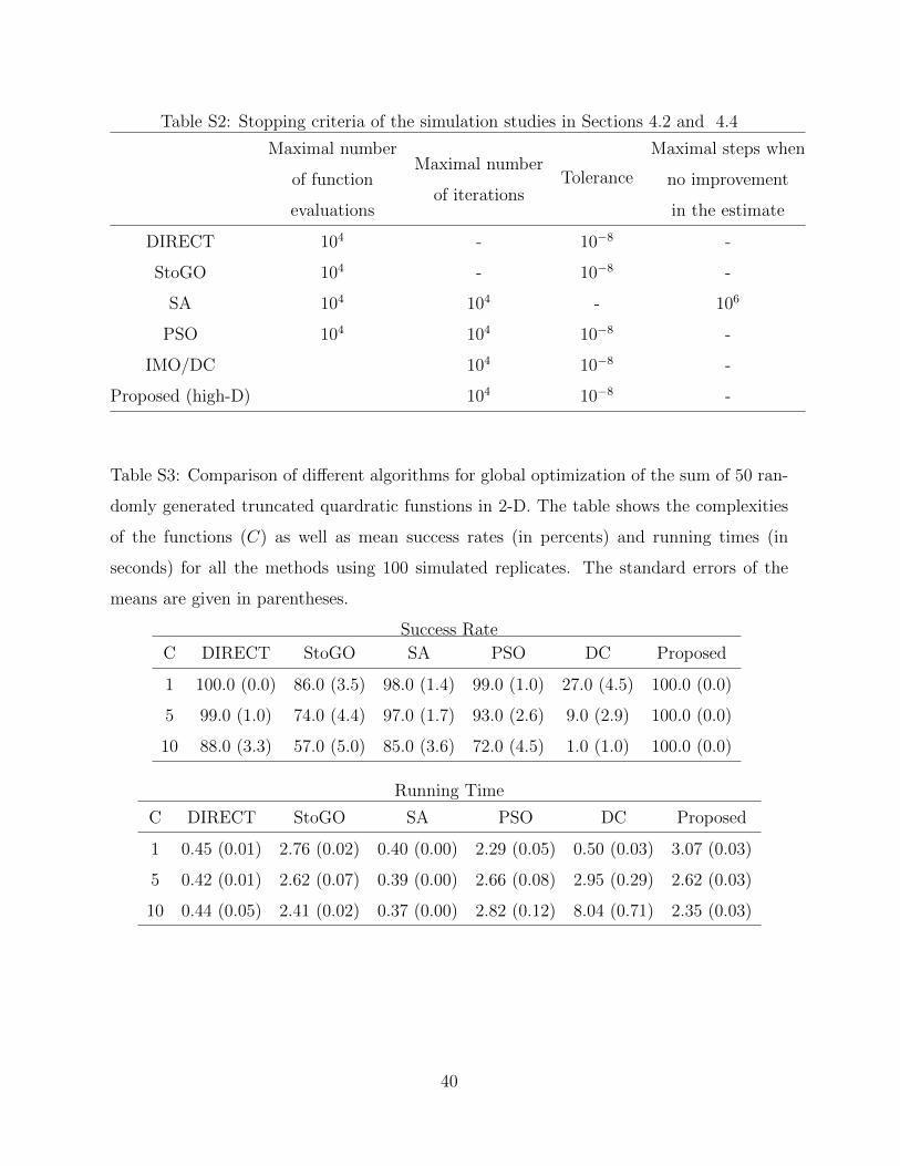
Table S2: Stopping criteria of the simulation studies in Sections 4.2 and 4.4
Maximal number
of function
evaluations
Maximal number
of iterationsTolerance
Maximal steps when
no improvement
in the estimate
DIRECT 104 - 10−8 -
StoGO 104 - 10−8 -
SA 104 104 - 106
PSO 104 104 10−8 -
IMO/DC 104 10−8 -
Proposed (high-D) 104 10−8 -
Table S3: Comparison of different algorithms for global optimization of the sum of 50 ran-
domly generated truncated quardratic funstions in 2-D. The table shows the complexities
of the functions (C) as well as mean success rates (in percents) and running times (in
seconds) for all the methods using 100 simulated replicates. The standard errors of the
means are given in parentheses.
Success Rate
C DIRECT StoGO SA PSO DC Proposed
1 100.0 (0.0) 86.0 (3.5) 98.0 (1.4) 99.0 (1.0) 27.0 (4.5) 100.0 (0.0)
5 99.0 (1.0) 74.0 (4.4) 97.0 (1.7) 93.0 (2.6) 9.0 (2.9) 100.0 (0.0)
10 88.0 (3.3) 57.0 (5.0) 85.0 (3.6) 72.0 (4.5) 1.0 (1.0) 100.0 (0.0)
Running Time
C DIRECT StoGO SA PSO DC Proposed
1 0.45 (0.01) 2.76 (0.02) 0.40 (0.00) 2.29 (0.05) 0.50 (0.03) 3.07 (0.03)
5 0.42 (0.01) 2.62 (0.07) 0.39 (0.00) 2.66 (0.08) 2.95 (0.29) 2.62 (0.03)
10 0.44 (0.05) 2.41 (0.02) 0.37 (0.00) 2.82 (0.12) 8.04 (0.71) 2.35 (0.03)
40