Ming Li Canada Research Chair in Bioinformatics

Computer Science. U. Waterloo

Modern Homology Search

I want to show you how one simple theoretical idea can make big impact to a practical field.

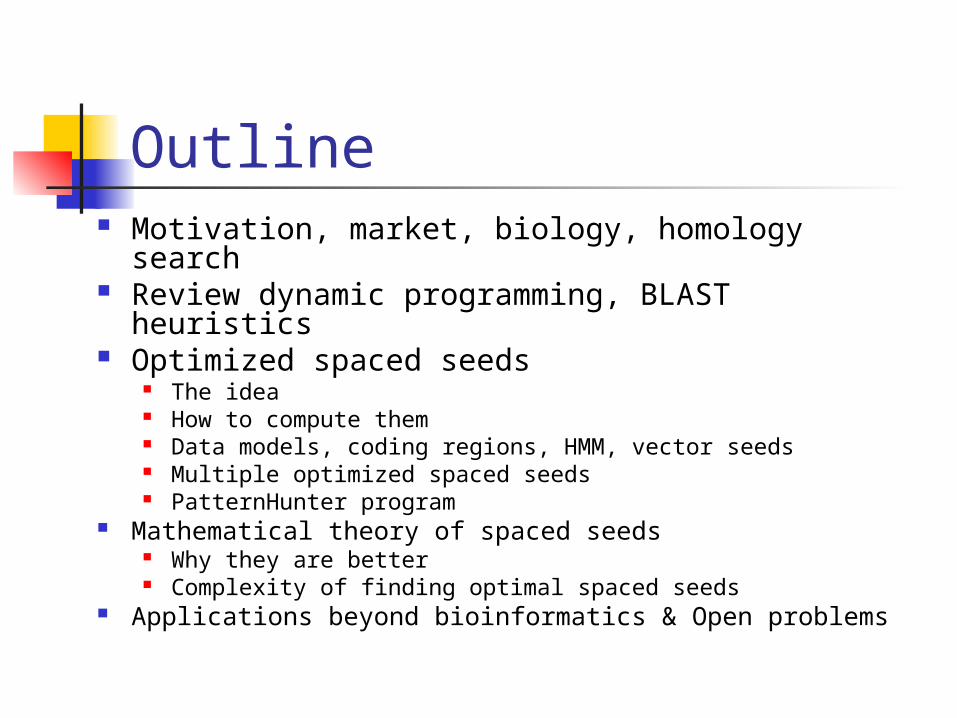
Outline Motivation, market, biology, homology search Review dynamic programming, BLAST heuristics Optimized spaced seeds

The idea How to compute them Data models, coding regions, HMM, vector seeds Multiple optimized spaced seeds PatternHunter program

Mathematical theory of spaced seeds Why they are better Complexity of finding optimal spaced seeds

Applications beyond bioinformatics & Open problems

1. Introduction Biology Motivation and market Definition of homology search

problem

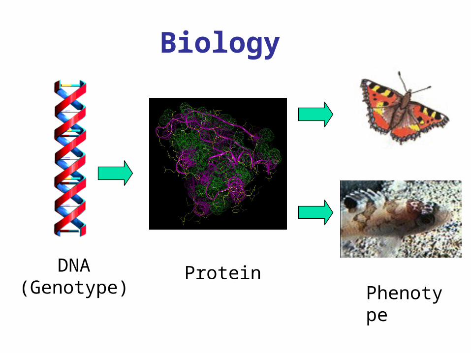
Biology

ProteinPhenotype

DNA(Genotype)

A T

T A

C

C

C

C

G

G

G

G

G

T

T

T

A

A

A

A

T

C

A T

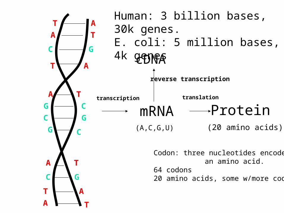
mRNA Proteintranscription translation

Human: 3 billion bases, 30k genes.E. coli: 5 million bases, 4k genes

(A,C,G,U) (20 amino acids)

Codon: three nucleotides encode an amino acid.64 codons20 amino acids, some w/more codes

cDNAreverse transcription

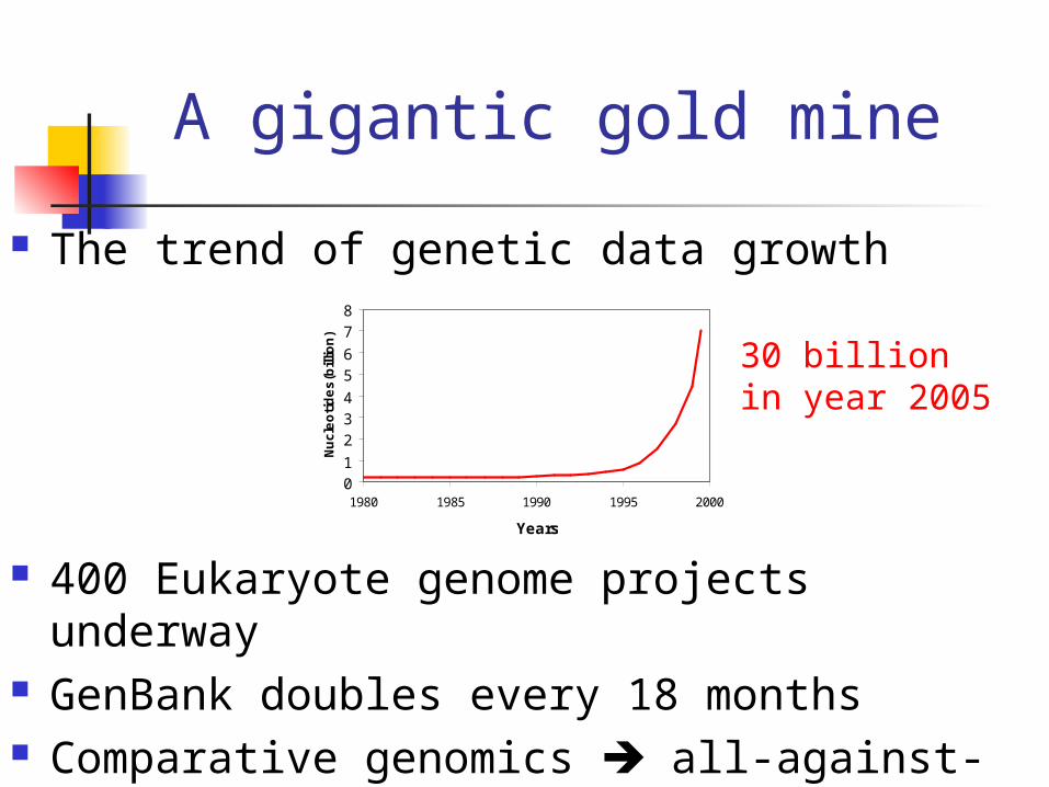
A gigantic gold mine

The trend of genetic data growth

400 Eukaryote genome projects underway GenBank doubles every 18 months Comparative genomics all-against-all

search Software must be scalable to large

datasets.

01

234

56

78

1980 1985 1990 1995 2000

Years

Nu

cle

oti

de

s(b

illio

n)

30 billionin year 2005

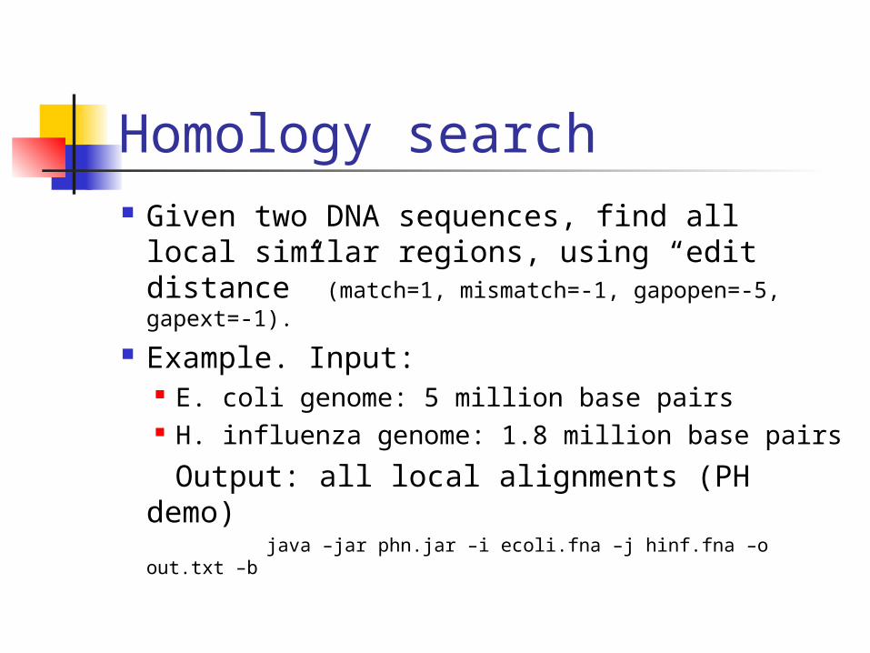
Homology search Given two DNA sequences, find all local

similar regions, using “edit distance” (match=1, mismatch=-1, gapopen=-5, gapext=-1).

Example. Input: E. coli genome: 5 million base pairs H. influenza genome: 1.8 million base pairs

Output: all local alignments (PH demo) java –jar phn.jar –i ecoli.fna –j hinf.fna –o out.txt –b

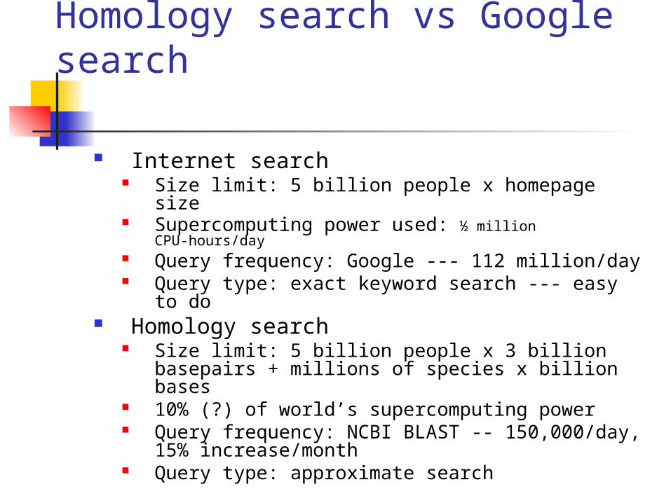
Homology search vs Google search

Internet search Size limit: 5 billion people x homepage size Supercomputing power used: ½ million CPU-

hours/day Query frequency: Google --- 112 million/day Query type: exact keyword search --- easy to

do Homology search

Size limit: 5 billion people x 3 billion basepairs + millions of species x billion bases

10% (?) of world’s supercomputing power Query frequency: NCBI BLAST -- 150,000/day,

15% increase/month Query type: approximate search

Bioinformatics Companies living on Blast Paracel (Celera)

TimeLogic (recently liquidated)

TurboGenomics (TurboWorx)

NSF, NIH, pharmaceuticals proudly support many supercomputing centers mainly for homology search

Hardware high cost & become obsolete in 2 years.

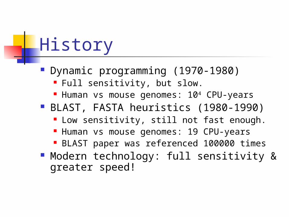
History Dynamic programming (1970-1980)

Full sensitivity, but slow. Human vs mouse genomes: 104 CPU-years

BLAST, FASTA heuristics (1980-1990) Low sensitivity, still not fast enough. Human vs mouse genomes: 19 CPU-years BLAST paper was referenced 100000 times

Modern technology: full sensitivity & greater speed!

2. Old Technology Dynamic programming – full

sensitivity homology search BLAST heuristics --- trading

sensitivity with time.

Dynamic Programming: Longest Common

Subsequence (LCS).

V=v1v2 … vn W=w1w2 … wm s(i,j) = length of LCS of V[1..i] and W[1..j] Dynamic Programming:

s(i-1,j)s(i,j)=max s(i,j-1)

s(i-1,j-1)+1,vi=wj

Sequence Alignment (Needleman-Wunsch, 1970)

s(i,j)=max s(i-1,j) + d(vi,-)

s(i,j-1)+d(-,wj) s(i-1,j-1)+d(vi,wj) 0 (Smith-Waterman, 1981)

* No affine gap penalties,

where d, for proteins, is either PAM or BLOSUM matrix. For DNA, it can be: match 1, mismatch -1, gap -3 (In fact: open gap -5, extension -1.)

d(-,x)=d(x,-)= -a, d(x,y)=-u. When a=0, u=infinity, it is LCS.

Misc. Concerns

Local sequence alignment, add s[i,j]=0. Gap penalties. For good reasons, we charge

first gap cost a, and then subsequent continuous insertions b<a.

Space efficient sequence alignment. Hirschberg alg. in O(n2) time, O(n) space.

Multiple alignment of k sequences: O(nk)

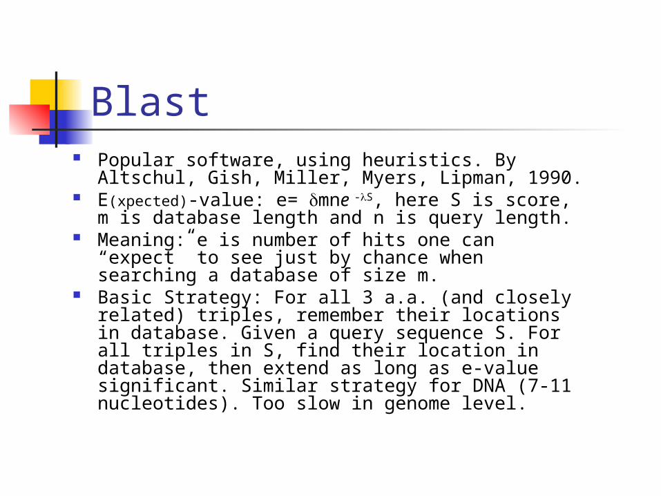
Blast Popular software, using heuristics. By Altschul, Gish,

Miller, Myers, Lipman, 1990. E(xpected)-value: e= mne -S, here S is score, m is

database length and n is query length. Meaning: e is number of hits one can “expect” to see

just by chance when searching a database of size m. Basic Strategy: For all 3 a.a. (and closely related)

triples, remember their locations in database. Given a query sequence S. For all triples in S, find their location in database, then extend as long as e-value significant. Similar strategy for DNA (7-11 nucleotides). Too slow in genome level.

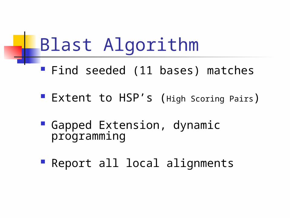
Blast Algorithm Find seeded (11 bases) matches

Extent to HSP’s (High Scoring Pairs)

Gapped Extension, dynamic programming

Report all local alignments

BLAST Algorithm Example: Find seeded matches of 11 base pairs Extend each match to right and left,

until the scores drop too much, to form an alignment

Report all local alignments

Example: AGCGATGTCACGCGCCCGTATTTCCGTA TCGGATCTCACGCGCCCGGCTTACCGTG

| | | | | | | | | | | | | | | | | | | |Gx

0 0 0 1 1 1 0 1 1 1 1 1 1 1 1 1 1 1 0 0 1 1 0 1 1 1 1 0

BLAST Dilemma: If you want to speed up, have to

use a longer seed. However, we now face a dilemma: increasing seed size speeds up, but

loses sensitivity; decreasing seed size gains sensitivity,

but loses speed. How do we increase sensitivity &

speed simultaneously? For 20 years, many tried: suffix tree, better programming ..

3. Optimized Spaced Seeds Why are they better How to compute them Data models, coding regions, HMM PatternHunter Multiple spaced seeds Vector seeds

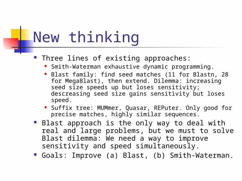
New thinking Three lines of existing approaches:

Smith-Waterman exhaustive dynamic programming. Blast family: find seed matches (11 for Blastn, 28 for

MegaBlast), then extend. Dilemma: increasing seed size speeds up but loses sensitivity; descreasing seed size gains sensitivity but loses speed.

Suffix tree: MUMmer, Quasar, REPuter. Only good for precise matches, highly similar sequences.

Blast approach is the only way to deal with real and large problems, but we must to solve Blast dilemma: We need a way to improve sensitivity and speed simultaneously.

Goals: Improve (a) Blast, (b) Smith-Waterman.

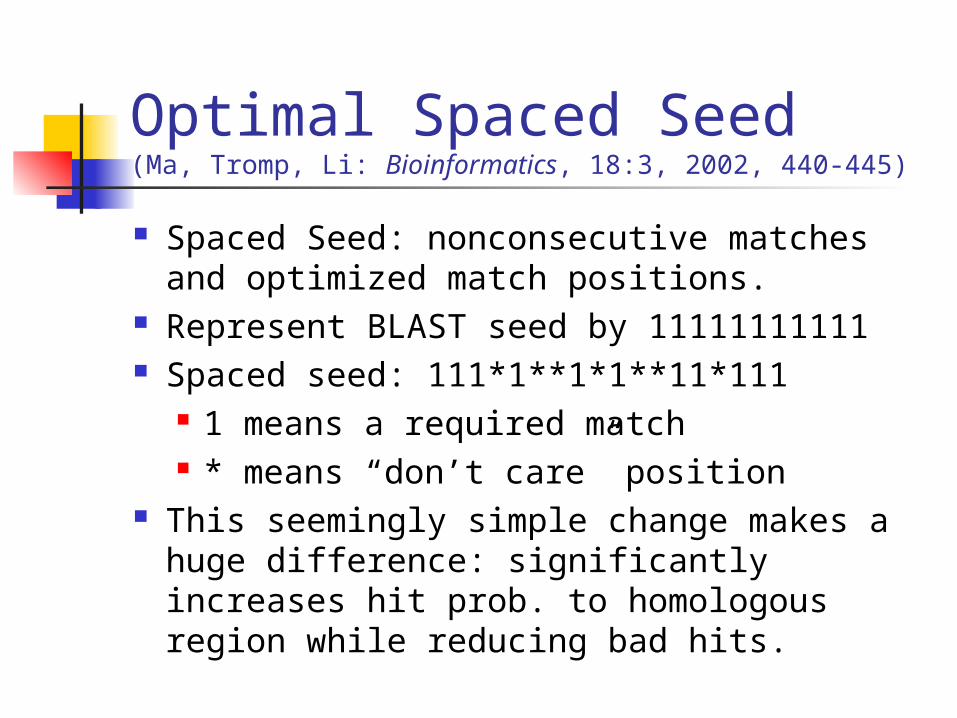
Optimal Spaced Seed(Ma, Tromp, Li: Bioinformatics, 18:3, 2002, 440-445)

Spaced Seed: nonconsecutive matches and optimized match positions.

Represent BLAST seed by 11111111111 Spaced seed: 111*1**1*1**11*111

1 means a required match * means “don’t care” position

This seemingly simple change makes a huge difference: significantly increases hit prob. to homologous region while reducing bad hits.

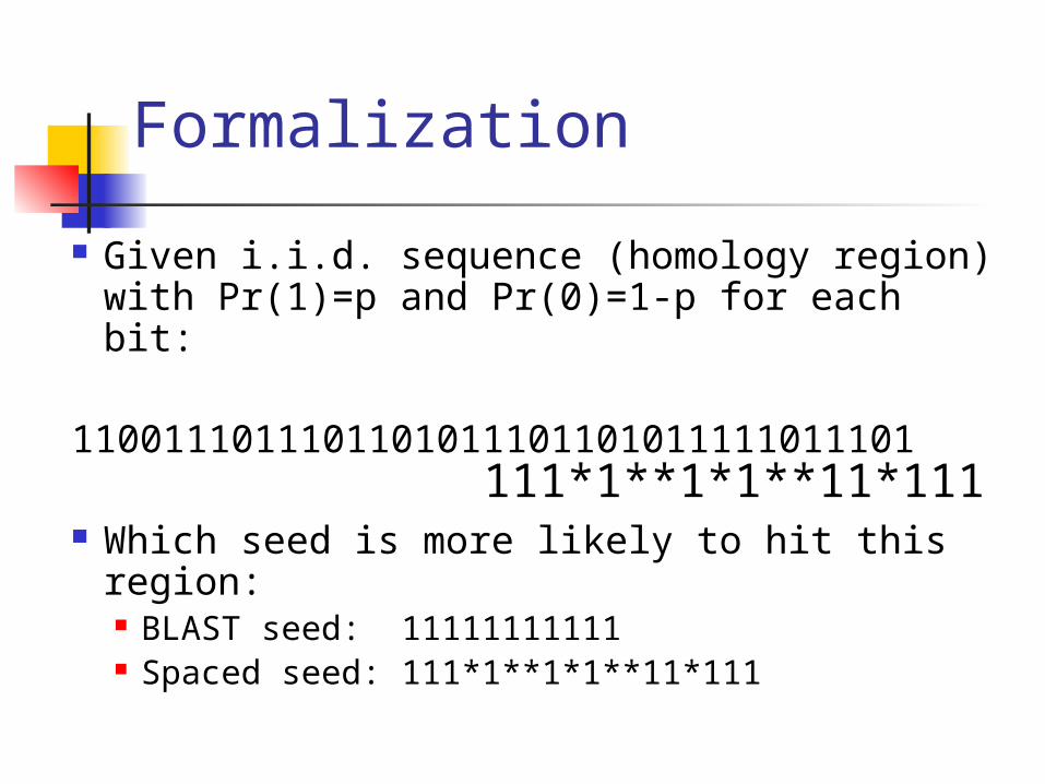
Formalization

Given i.i.d. sequence (homology region) with Pr(1)=p and Pr(0)=1-p for each bit:

1100111011101101011101101011111011101

Which seed is more likely to hit this region: BLAST seed: 11111111111 Spaced seed: 111*1**1*1**11*111

111*1**1*1**11*111

Sensitivity: PH weight 11 seed vs Blast 11 & 10

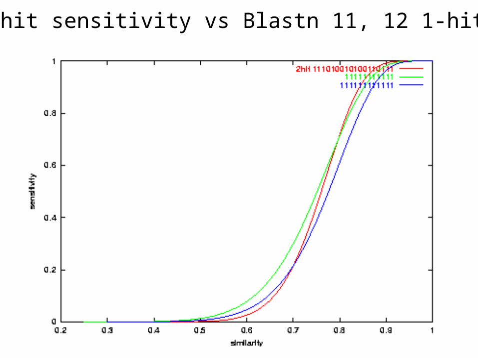
PH 2-hit sensitivity vs Blastn 11, 12 1-hit

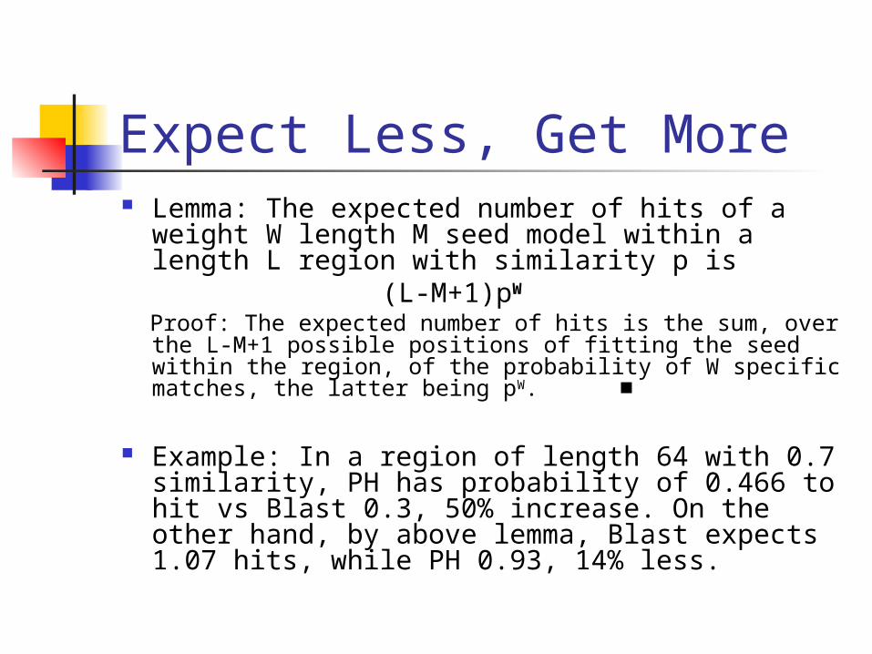
Expect Less, Get More Lemma: The expected number of hits of a

weight W length M seed model within a length L region with similarity p is

(L-M+1)pW

Proof: The expected number of hits is the sum, over the L-M+1 possible positions of fitting the seed within the region, of the probability of W specific matches, the latter being pW. ■

Example: In a region of length 64 with 0.7 similarity, PH has probability of 0.466 to hit vs Blast 0.3, 50% increase. On the other hand, by above lemma, Blast expects 1.07 hits, while PH 0.93, 14% less.

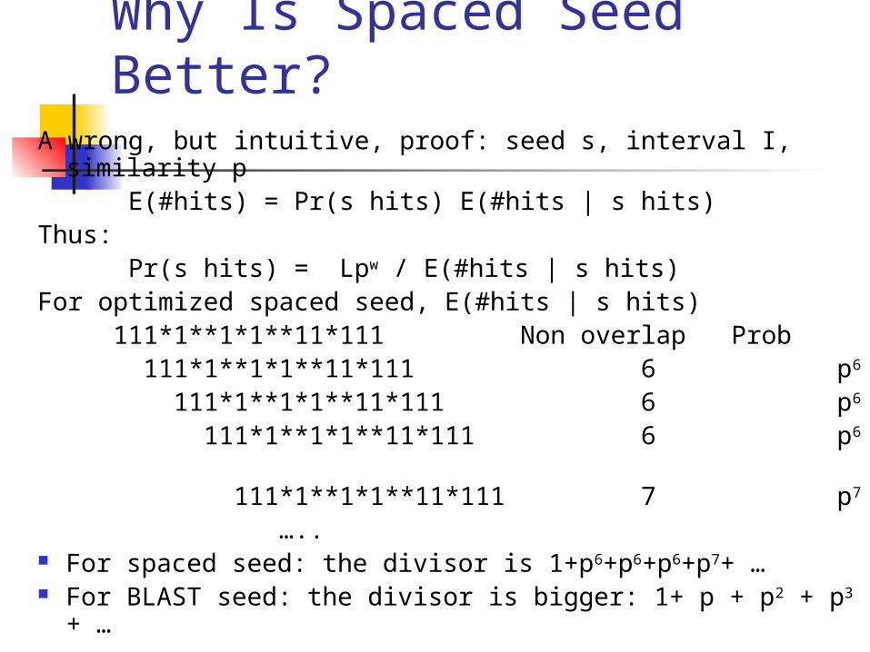
Why Is Spaced Seed Better?

A wrong, but intuitive, proof: seed s, interval I, similarity p

E(#hits) = Pr(s hits) E(#hits | s hits)Thus: Pr(s hits) = Lpw / E(#hits | s hits)For optimized spaced seed, E(#hits | s hits) 111*1**1*1**11*111 Non overlap Prob 111*1**1*1**11*111 6 p6

111*1**1*1**11*111 6 p6

111*1**1*1**11*111 6 p6 111*1**1*1**11*111 7 p7

….. For spaced seed: the divisor is 1+p6+p6+p6+p7+ … For BLAST seed: the divisor is bigger: 1+ p + p2 + p3 +

…

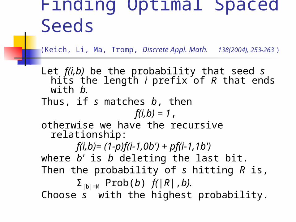
Finding Optimal Spaced Seeds(Keich, Li, Ma, Tromp, Discrete Appl. Math. 138(2004), 253-263 )

Let f(i,b) be the probability that seed s hits the length i prefix of R that ends with b.

Thus, if s matches b, then f(i,b) = 1,otherwise we have the recursive

relationship: f(i,b)= (1-p)f(i-1,0b') + pf(i-1,1b')where b' is b deleting the last bit. Then the probability of s hitting R is, Σ|b|=M Prob(b) f(|R|,b).Choose s with the highest probability.

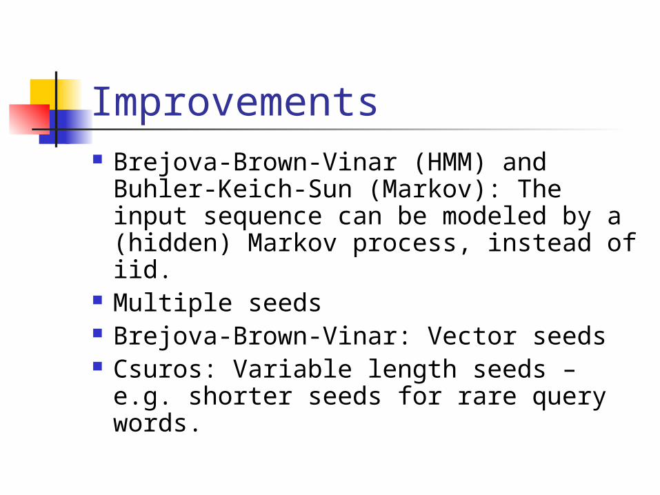
Improvements Brejova-Brown-Vinar (HMM) and

Buhler-Keich-Sun (Markov): The input sequence can be modeled by a (hidden) Markov process, instead of iid.

Multiple seeds Brejova-Brown-Vinar: Vector seeds Csuros: Variable length seeds – e.g.

shorter seeds for rare query words.

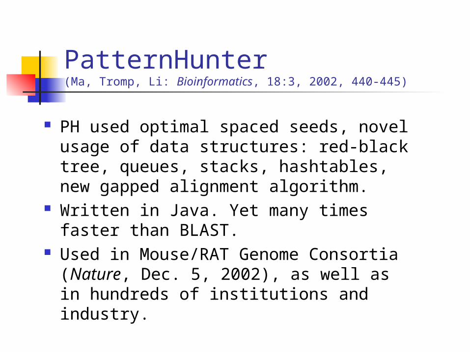
PatternHunter(Ma, Tromp, Li: Bioinformatics, 18:3, 2002, 440-445)

PH used optimal spaced seeds, novel usage of data structures: red-black tree, queues, stacks, hashtables, new gapped alignment algorithm.

Written in Java. Yet many times faster than BLAST.

Used in Mouse/RAT Genome Consortia (Nature, Dec. 5, 2002), as well as in hundreds of institutions and industry.

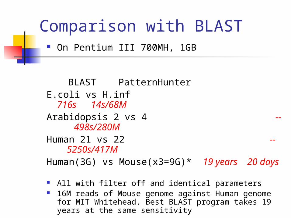
Comparison with BLAST On Pentium III 700MH, 1GB

BLAST PatternHunter

E.coli vs H.inf 716s 14s/68MArabidopsis 2 vs 4 --

498s/280MHuman 21 vs 22 --

5250s/417MHuman(3G) vs Mouse(x3=9G)* 19 years 20

days

All with filter off and identical parameters 16M reads of Mouse genome against Human genome

for MIT Whitehead. Best BLAST program takes 19 years at the same sensitivity

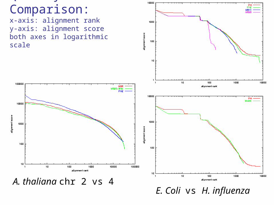
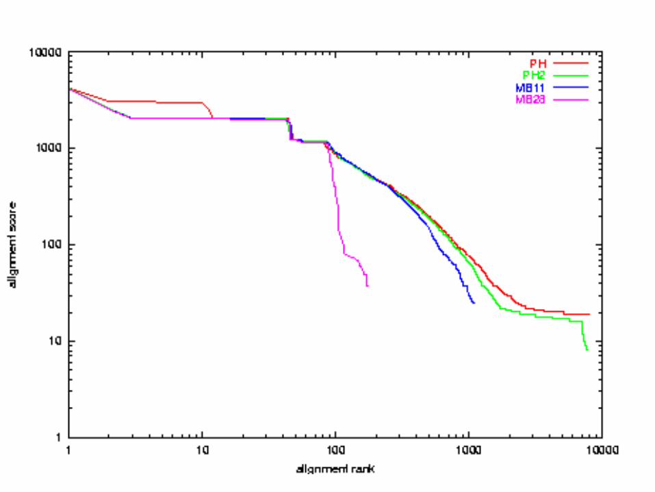
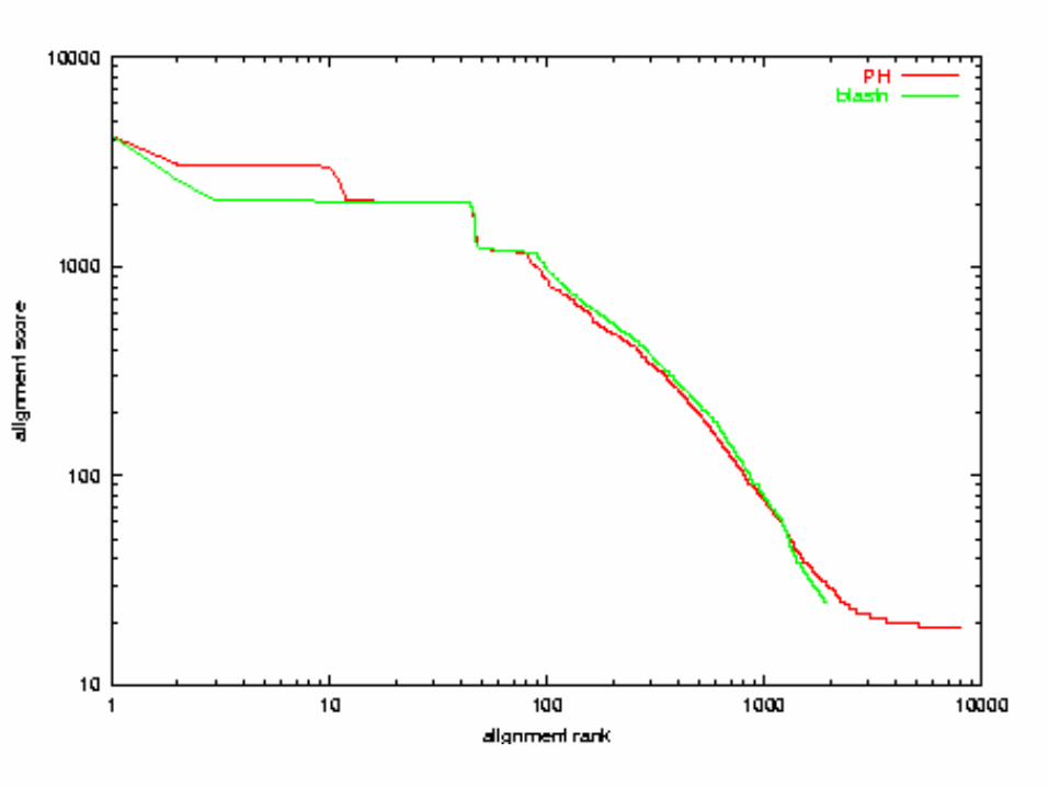
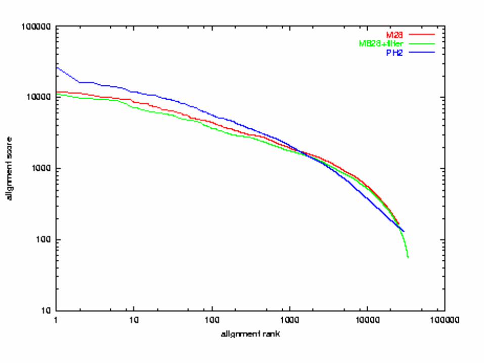
Quality Comparison:x-axis: alignment ranky-axis: alignment scoreboth axes in logarithmic scale

A. thaliana chr 2 vs 4E. Coli vs H. influenza

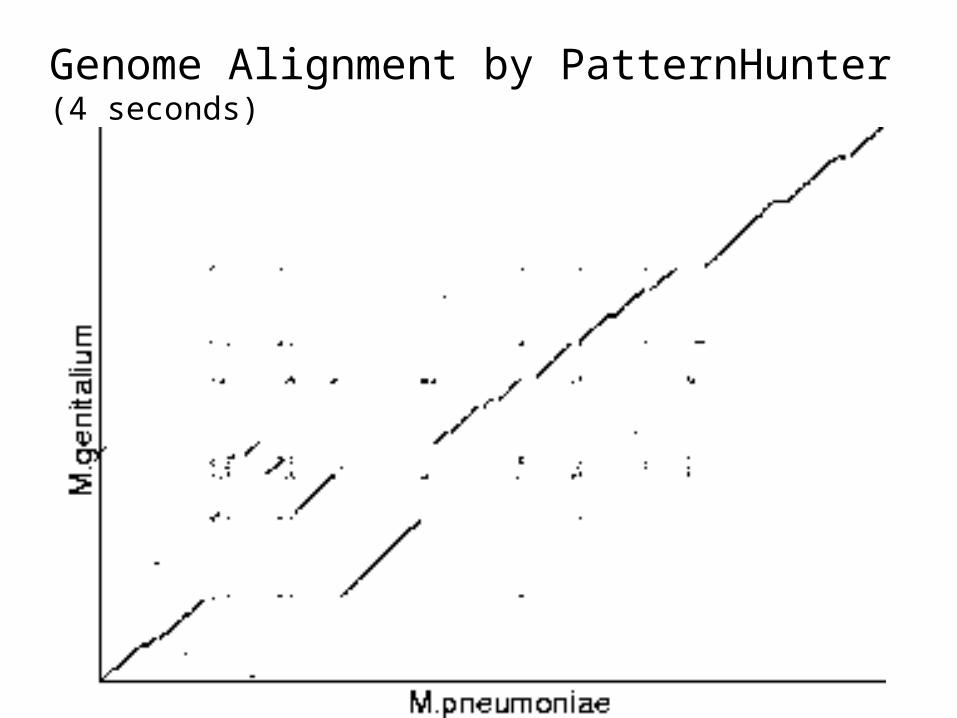
Genome Alignment by PatternHunter (4 seconds)

Prior Literature Over the years, it turns out, that the

mathematicians know about certain patterns appear more likely than others: for example, in a random English text, ABC is more likely to appear than AAA, in their study of renewal theory.

Random or multiple spaced q-grams were used in the following work:

FLASH by Califano & Rigoutsos Multiple filtration by Pevzner & Waterman LSH of Buhler Praparata et al

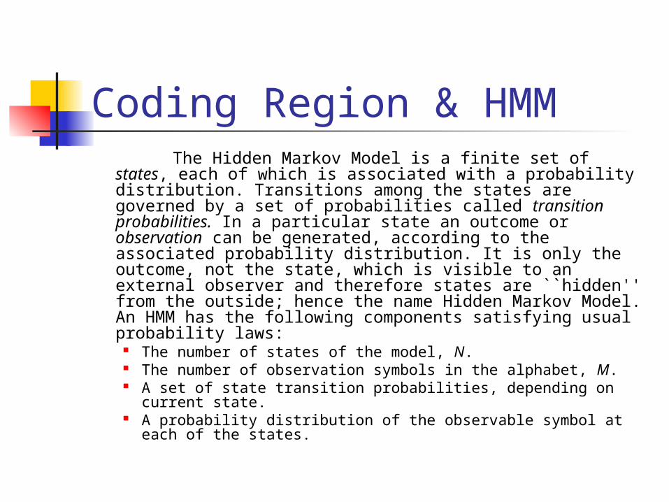
Coding Region & HMM The Hidden Markov Model is a finite set of states, each

of which is associated with a probability distribution. Transitions among the states are governed by a set of probabilities called transition probabilities. In a particular state an outcome or observation can be generated, according to the associated probability distribution. It is only the outcome, not the state, which is visible to an external observer and therefore states are ``hidden'' from the outside; hence the name Hidden Markov Model. An HMM has the following components satisfying usual probability laws:

The number of states of the model, N. The number of observation symbols in the alphabet, M. A set of state transition probabilities, depending on current

state. A probability distribution of the observable symbol at each of

the states.

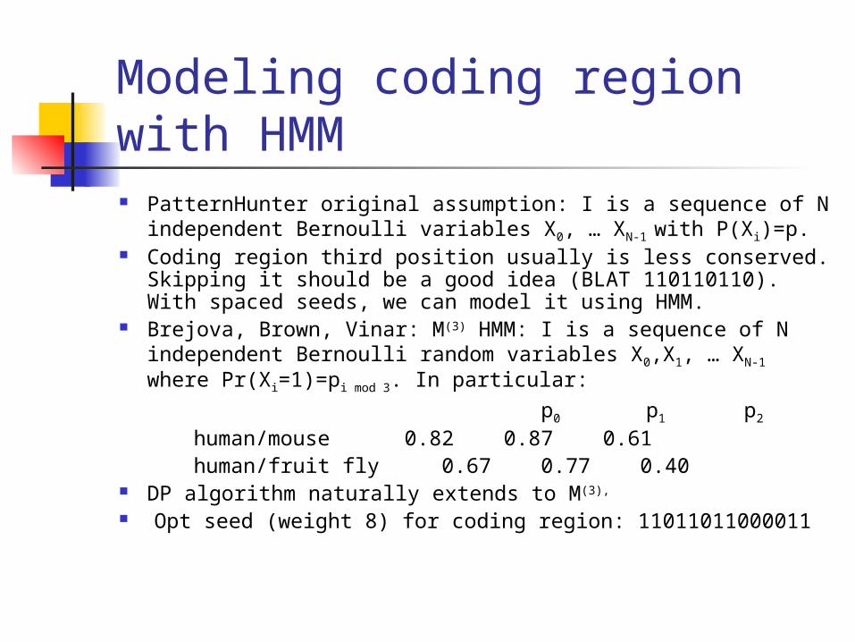
Modeling coding region with HMM PatternHunter original assumption: I is a sequence of N

independent Bernoulli variables X0, … XN-1 with P(Xi)=p. Coding region third position usually is less conserved.

Skipping it should be a good idea (BLAT 110110110). With spaced seeds, we can model it using HMM.

Brejova, Brown, Vinar: M(3) HMM: I is a sequence of N independent Bernoulli random variables X0,X1, … XN-1 where Pr(Xi=1)=pi mod 3. In particular:

p0 p1 p2

human/mouse 0.82 0.87 0.61 human/fruit fly 0.67 0.77 0.40 DP algorithm naturally extends to M(3),

Opt seed (weight 8) for coding region: 11011011000011

Figures from Brejova-Brown-Vinar

Picture of M(3)

Extending M(3), Brejova-Brown-Vinar proposed M(8), above, to modeldependencies among positions within codons: Σpijk = 1, each codon has conservation pattern ijk with probability pijk.

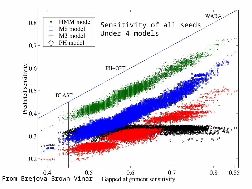
From Brejova-Brown-Vinar

Sensitivity of all seeds Under 4 models

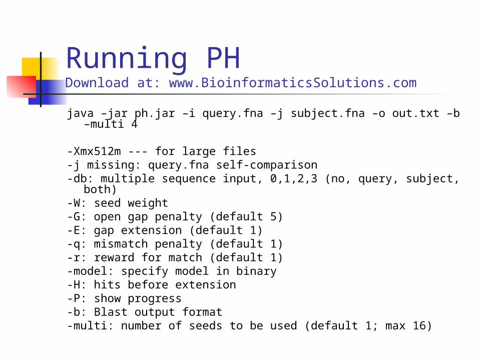
Running PHDownload at: www.BioinformaticsSolutions.com

java –jar ph.jar –i query.fna –j subject.fna –o out.txt –b –multi 4

-Xmx512m --- for large files-j missing: query.fna self-comparison-db: multiple sequence input, 0,1,2,3 (no, query, subject, both)-W: seed weight-G: open gap penalty (default 5)-E: gap extension (default 1)-q: mismatch penalty (default 1)-r: reward for match (default 1)-model: specify model in binary-H: hits before extension-P: show progress-b: Blast output format-multi: number of seeds to be used (default 1; max 16)

Multiple Spaced Seeds: Approaching Smith-Waterman Sensitivity(Li, Ma, Kisman, Tromp, PatternHunter II, J. Bioinfo Comput. Biol. 2004)

The biggest problem for Blast was low sensitivity (and low speed). Massive parallel machines are built to do Smith-Waterman exhaustive dynamic programming.

Spaced seeds give PH a unique opportunity of using several optimal seeds to achieve optimal sensitivity, this was not possible for Blast technology.

Economy --- 2 seeds (½ time slow down) achieve sensitivity of 1 seed of shorter length (4 times speed).

With multiple optimal seeds. PH II approaches Smith-Waterman sensitivity, and 3000 times faster.

Finding optimal seeds, even one, is NP-hard. Experiment: 29715 mouse EST, 4407 human EST.

Sensitivity and speed comparison next two slides.

Finding Multiple Seeds (PH II)

Computing the hit probability of given k seeds on a uniformly distributed random region is NP-hard.

Finding a set of k optimal seeds to maximize the hit probability cannot be approximated within 1-1/e unless NP=P

Given k seeds, algorithm DP can be adapted to compute their sensitivity (probability one of the seeds has a hit).

Greedy Strategy Compute one optimal seed a. S={a} Given S, find b maximizing hit probability of S U {b}. Coding region, use M(3), 0.8, 0.8, 0.5 (for mod 3 positions)

We took 12 CPU-days on 3GHz PC to compute 16 weight 11 seeds. General seeds (first 4): 111010010100110111, 111100110010100001011, 11010000110001010111, 1110111010001111.

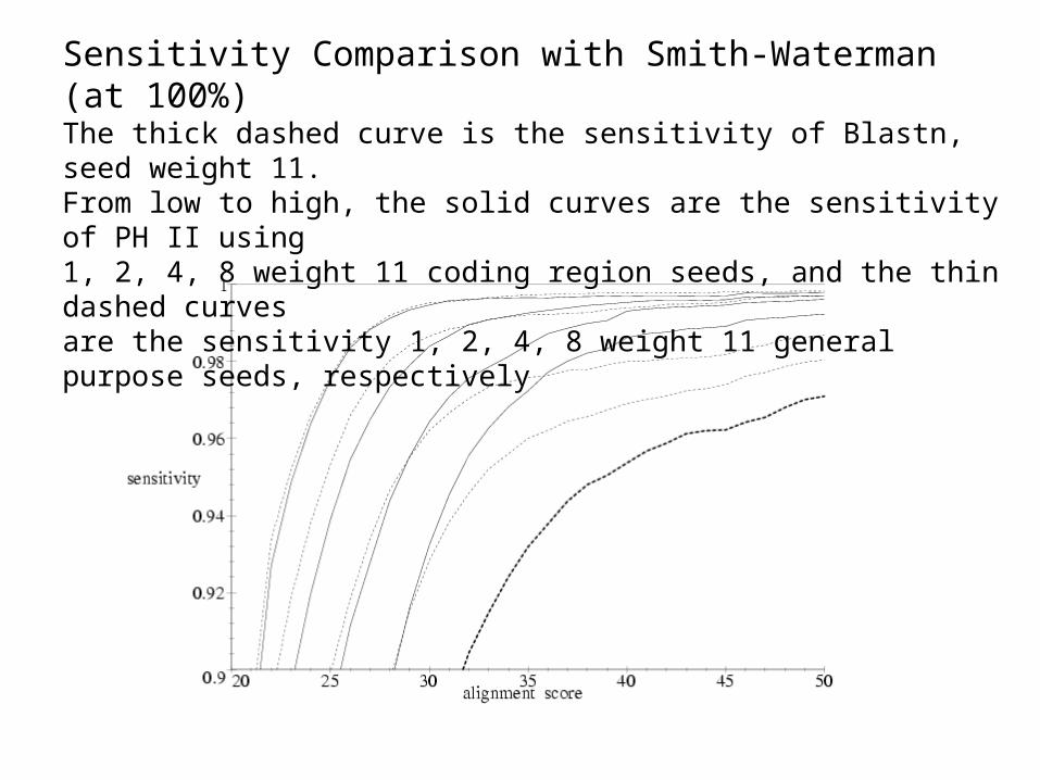
Sensitivity Comparison with Smith-Waterman (at 100%)The thick dashed curve is the sensitivity of Blastn, seed weight 11. From low to high, the solid curves are the sensitivity of PH II using 1, 2, 4, 8 weight 11 coding region seeds, and the thin dashed curves are the sensitivity 1, 2, 4, 8 weight 11 general purpose seeds, respectively

Speed Comparison with Smith-Waterman

Smith-Waterman (SSearch): 20 CPU-days.

PatternHunter II with 4 seeds: 475 CPU-seconds. 3638 times faster than Smith-Waterman dynamic programming at the same sensitivity.

Vector SeedsDefinition. A vector seed is an ordered pair Q=(w,T),

where w is a weight vector (w1, … wM) and T is a threshold value. An alignment sequence x1,…,xn contains a hit of the seed Q at position k if

i=1..M(wi∙xk+i-1) ≥ T

The number of nonzero positions in w is called the support of the seed.

Comments. Other seeds are special cases of vector seeds.

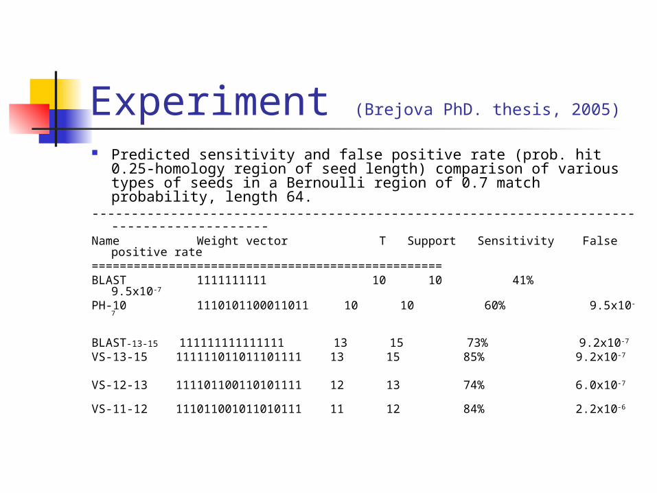
Experiment (Brejova PhD. thesis, 2005)

Predicted sensitivity and false positive rate (prob. hit 0.25-homology region of seed length) comparison of various types of seeds in a Bernoulli region of 0.7 match probability, length 64.

-----------------------------------------------------------------------------------------Name Weight vector T Support Sensitivity False positive

rate===============================================

===BLAST 1111111111 10 10 41% 9.5x10-7

PH-10 1110101100011011 10 10 60% 9.5x10-7

BLAST-13-15 111111111111111 13 15 73% 9.2x10-7

VS-13-15 111111011011101111 13 15 85% 9.2x10-7

VS-12-13 111101100110101111 12 13 74% 6.0x10-7

VS-11-12 111011001011010111 11 12 84% 2.2x10-6

Variable weight spaced seeds M. Csuros proposal: use variable

weighted spaced seeds depending on the composition of the strings to be hashed. Rarer strings are expected to produce fewer false positives, use seeds with smaller weight --- this increases the sensitivity.

Open Question Can we use different patterns (of same

weight) at different positions. So this can be called variable position-spaced seeds. At the same weight, we do not increase expected number of false positive hits. Can we increase sensitivity? Find these patterns? How much increase will there be? Practical enough?

If the above is not the case, then prove: single optimal seed is always better than variable positions.

Old field, new trend Research trend

Dozens of papers on spaced seeds have appeared since the original PH paper, in 3 years.

Many more have used PH in their work. Most modern alignment programs (including

BLAST) have now adopted spaced seeds Spaced seeds are serving thousands of users/day

PatternHunter direct users Pharmaceutical/biotech firms. Mouse Genome Consortium, Nature, Dec. 5,

2002. Hundreds of academic institutions.

4. Mathematical Theory of spaced seeds Why they are better: Spaced seeds hits first Asymptotic sensitivity: is there a “best seed”

in absolute sense? NP hardness of computing sensitivity Approximation algorithm for sensitivity

Why are the spaced seeds better

Theorem 1. Let I be a homologous region, homology level p. For any sequence 0≤i0 < i1 … < in-1 ≤ |I|-|s|, let Aj be the event a spaced seed s hits I at ij, Bj be

event the consecutive seed hits I at j. (Keich, Li, Ma, Tromp, Discrete Appl. Math. 138(2004), 253-263 )

(1) P(Uj<n Aj) ≥ P(Uj<n Bj); When ij=j, “>” holds.Proof. Induction on n. For n=1, P(A0)=pW=P(B0). Assume the theorem holds for n≤N, we

prove it holds for N+1. Let Ek denote the event that, when putting a seed at I[0], 0th, 1st … k-1st 1s in the seed all match & the k-th 1 mismatches. Clearly, Ek is a partition of sample space for all k=0, .. , W, and P(Ek)=pk(1-p) for any seed. (Note, Ek for Ai and Ek for Bi have different indices – they are really different events.) It is sufficient to show, for each k≤W:

(2) P(Uj=0..N Aj|Ek)≥P(Uj=0..NBj|Ek)

When k=W, both sides of (2) equal to 1. For k<W since (Uj≤kBj)∩Ek=Φ and {Bk+1,Bk+2, … BN} are mutually independent of Ek, we have

(3) P(Uj=0..NBj|Ek)=P(Uj=k+1..NBj)

Now consider the first term in (2). For each k in {0, … W-1}, at most k+1 of the events Aj

satisfy Aj∩Ek=Φ because Aj∩Ek=Φ iff when aligned at ij seed s has a 1 bit at overlapping k-th bit when the seed was at 0 – there are at most k+1 choices. Thus, there exist indices 0<mk+1<mk+2 … <mN ≤N such that Amj∩Ek≠Φ. Since Ek means all previous bits matched (except for k-th), it is clear that Ek is non-negatively correlated with Uj=k+1..N Amj, thus

(4) P(Uj=0..N Aj|Ek)≥P(Uj=k+1..N Amj|Ek)≥P(Uj=k+1..NAmj)

By the inductive hypothesis, we have

P(Uj=k+1..N Amj) ≥ P(Uj=k+1..NBj)

Combined with (3),(4), this proves (2), hence the “≥ part” of (1) of the theorem.

To prove when ij=j, P(Uj=0..n-1Aj)>P(Uj=0..n-1Bj) --- (5)

We prove (5) by induction on n. For n=2, we have

P(Uj=0,1Aj)=2pw – p2w-Shift1>2pw-pw+1=P(Uj=0,1Bj) (*)

where shift1=number of overlapped bits of the spaced seed s when shifted to the right by 1 bit.

For inductive step, note that the proof of (1) shows that for all k=0,1, … ,W, P(Uj=0..n-1Aj|Ek)≥P(Uj=0..n-1Bj|Ek). Thus to prove (5) we only need to prove that

P(Uj=0..n-1Aj|E0)>P(Uj=0..n-1Bj|E0).

The above follows from the inductive hypothesis as follows: P(Uj=0..n-1Aj|E0)=P(Uj=1..n-1Aj)>P(Uj=1..n-1Bj)=P(Uj=0..n-1Bj|E0). ■

CorollaryCorollary: Assume I is infinite. Let ps and pc be

the first positions a spaced seed and the consecutive seed hit I, respectively. Then E[ps] < E[pc].

Proof. E[ps]=Σk=0..∞ kP(ps=k)

=Σk=0..∞ k[P(ps>k-1)-P(ps>k)]

=Σk=0..∞P(ps>k)

=Σk=0..∞(1-P(Uj=0..kAj))

<Σk=0..∞(1-P(Uj=0..kBj))

=E[pc]. ■

Asymptotic sensitivity(Buhler-Keich-Sun, JCSS 2004, Li-Ma-Zhang, SODA’2006)

Theorem. Given a spaced seed s, the asymptotic hit probability on a homologous region R can be computed, up to a constant factor, in time exponentially proportional to |s|, but independent of |R|.

Proof. Let d be one plus the length of the maximum run of 0's in s. Let M'=|s|+d. Consider an infinite iid sequence R=R[1]R[2] ... , Prob(R[i]=1)=p.

Let T be set of all length |s| strings that do not dominate s (not matched by s).

Let Z[i,j] denote the event that s does not hit at any of the positions R[i], R[i+1], … , R[j]. For any ti T, let

xi(n) = P[Z[1,n] | R[n..n+|s|-1] = ti ] .

That is, xi(n) is the no-hit probability in the first n positions when they end with

ti. We now establish a relationship between xi(n) and xi

(n-M’) . Let

Ci,j = P[Z[n-M'+1,n] | ti at n, tj at n-M'] x P[tj at n-M' | ti at n].

Thus Ci,j is the probability of generating tj at position n-M' (from ti at n) times the probability not having a hit in a region of length |s|+M' beginning with tj and ending with ti. Especially Ci,j ≠ 0 for any nontrivial seed of length greater than 0 (because of M’ with d spacing).

Proof ContinuedThen, xi

(n) = j=1K P[Z[1,n-M'] | tj at n-M']

x P[tj at n-M' | ti at n] x P[Z[n-M'+1,n] | ti at n, tj at n-M'] = j=1

K P[Z[1,n-M'] | tj at n-M'] x Ci,j

= j=1K Ci,j xj

(n-M’)

Define the transition matrix C=(Ci,j). It is a K x K matrix. Let x(n) = (x1

(n), x2(n), … , xK

(n)). Then, assuming that M' divides n, x(n) = x(1) ◦ (CT)n/M’.Because Ci,j > 0 for all i,j, C is a positive matrix. The row sum of the

i-th row is the probability that a length-(|s|+M') region ending with ti does not have a hit. The row sum is lower bounded by (1-p)d (1-pW ), where (1-p)d is the probability of generating d 0's and 1-pW is the probability of generating a string in T. It is known that the largest eigenvalue of C is positive and unique, and is lower bounded by the smallest row sum and upper bounded the largest row sum of C. Let λ1>0 be the largest eigenvalue, and λ2, 0 < ||λ2|| < λ1 be the second largest. There is a unique eigenvector corresponding to λ1.

x(n) / ||x(n)|| = x(1) ◦ (CT )n/M’ / ||x(1) ◦ (CT)n/M’|| converges to the eigenvector corresponding to λ1. As λ1

n tends to zero, we can use standard techniques to normalize xn as

y(n) = x(n) / ||x(n)||2 and then x(n+M’) = C y(n) .

Proof Continued …Then (by power method) the Rayleigh quotient of

λ = (y(n))T C y(n) / (y(n))T y(n) = (y(n))T x(n+M’)

converges to λ1. The convergence speed depends on the ratio λ1/ |λ2|, it

is known that we can upper bound the second largest eigenvalue λ2 in a positive matrix by:

λ2 ≤ λ1 (K-1)/(K+1)

where K= maxi,j,k,l (Ci,j Ck,l / Ci,l Ck,j). For any i,j, we have

pa (1-p)b (1-p)d ≤ Ci,j ≤ pa (1-p)b

where a is the number of 1's in tj, b the number of 0's in tj. K = O(1/(1-p)d ).

As (1 - 1/K)K goes to 1/e, the convergence can be achieved in O(K) = O(1/(1-p)d ) steps. The time complexity is therefore upper bounded by an exponential function in |s|. QED

Theorem 2. It is NP hard to find the optimal seed(Li, Ma, Kisman, Tromp, J. Bioinfo Comput. Biol. 2004)

Proof. Reduction from 3-SAT. Given a 3-SAT instance C1 … Cn, on Boolean variables x1, … , xm, where Ci= l1 + l2 + l3, each l is some xi or its complement. We reduce this to seed selection problem. The required seed has weight W=m+2 and length L=2m+2, and is intended to be of the form 1(01+10)m1, a straightforward variable assignment encoding. The i-th pair of bits after the initial 1 is called the code for variable xi. A 01 code corresponds to setting xi true, while a 10 means false. To prohibit code 11, we introduce, for every 1 ≤ i ≤ m, a region

Ai=1 (11)i-101(11)m-i 10m+1 1(11)i-110(11)m-i 1.

Since the seed has m 0s, it cannot bridge the middle 0m+1 part, and is thus forced to hit at the start or at the end. This obviously rules out code 11 for variable x i. Code 00 automatically becomes ruled out as well, since the seed must distribute m 1s among all m codes. Finally, for each clause Ci, we introduce

Ri =1(11)a-1 c1(11)m-a 1 000 1(11)b-1c2(11)m-b 1 000 1(11)c-1c3(11)m-c 1.

The total length of Ri is (2m+2)+3+(2m+2)+3+(2m+2)=6m+12; it consists of three parts each corresponding to a literal in the constraint, with ci being the code for making that literal true.

Thus a seed hits Ri iff the assignment encoded by the seed satisfies Ci . ■

The complexity of computing spaced seed sensitivity

Theorem. It is also NP hard to compute sensitivity of a given seed. It remains to be NPC even in a uniform region, at any homology level p.

Proof. Very complicated. Omitted.

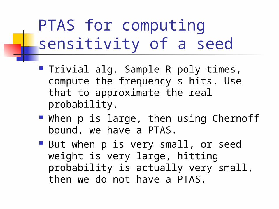
PTAS for computing sensitivity of a seed Trivial alg. Sample R poly times,

compute the frequency s hits. Use that to approximate the real probability.

When p is large, then using Chernoff bound, we have a PTAS.

But when p is very small, or seed weight is very large, hitting probability is actually very small, then we do not have a PTAS.

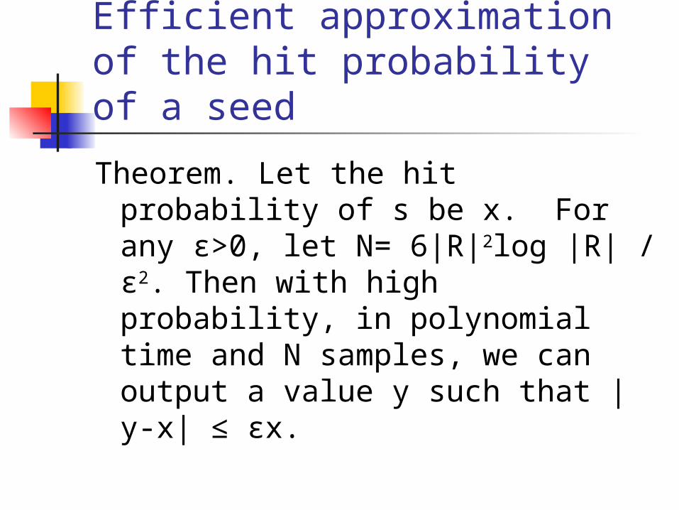
Efficient approximation of the hit probability of a seed

Theorem. Let the hit probability of s be x. For any ε>0, let N= 6|R|2log |R| / ε2. Then with high probability, in polynomial time and N samples, we can output a value y such that |y-x| ≤ εx.

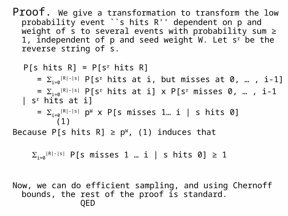
Proof. We give a transformation to transform the low probability event ``s hits R'' dependent on p and weight of s to several events with probability sum ≥ 1, independent of p and seed weight W. Let sr be the reverse string of s.

P[s hits R] = P[sr hits R] = i=0

|R|-|s| P[sr hits at i, but misses at 0, … , i-1]

= i=0|R|-|s| P[sr hits at i] x P[sr misses 0, … , i-1 | sr hits

at i] = i=0

|R|-|s| pW x P[s misses 1… i | s hits 0] (1)

Because P[s hits R] ≥ pW, (1) induces that i=0

|R|-|s| P[s misses 1 … i | s hits 0] ≥ 1

Now, we can do efficient sampling, and using Chernoff bounds, the rest of the proof is standard. QED

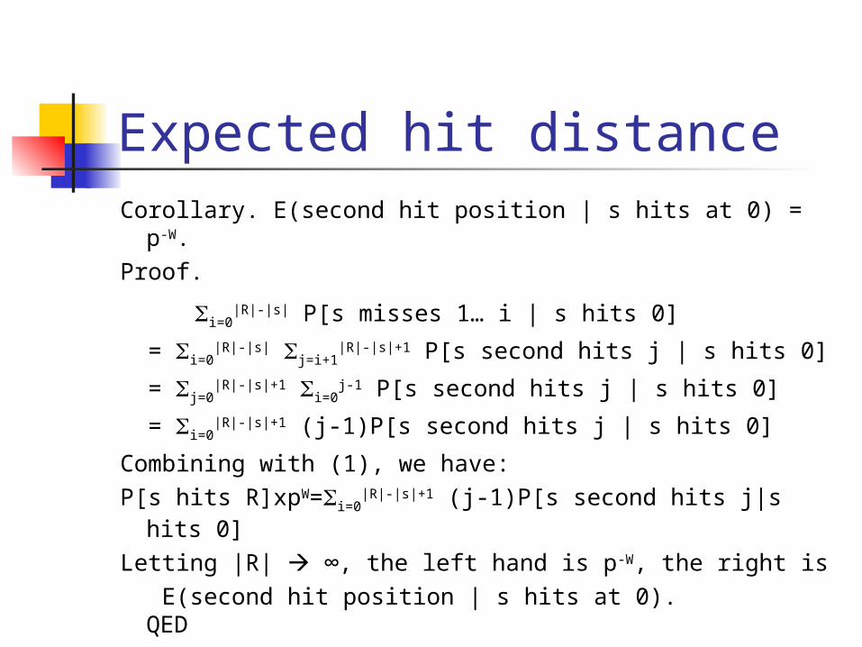
Expected hit distanceCorollary. E(second hit position | s hits at 0) = p-W.Proof.

i=0|R|-|s| P[s misses 1… i | s hits 0]

= i=0|R|-|s| j=i+1

|R|-|s|+1 P[s second hits j | s hits 0]

= j=0|R|-|s|+1 i=0

j-1 P[s second hits j | s hits 0]

= i=0|R|-|s|+1 (j-1)P[s second hits j | s hits 0]

Combining with (1), we have:P[s hits R]xpW=i=0

|R|-|s|+1 (j-1)P[s second hits j|s hits 0]

Letting |R| ∞, the left hand is p-W, the right is E(second hit position | s hits at 0). QED

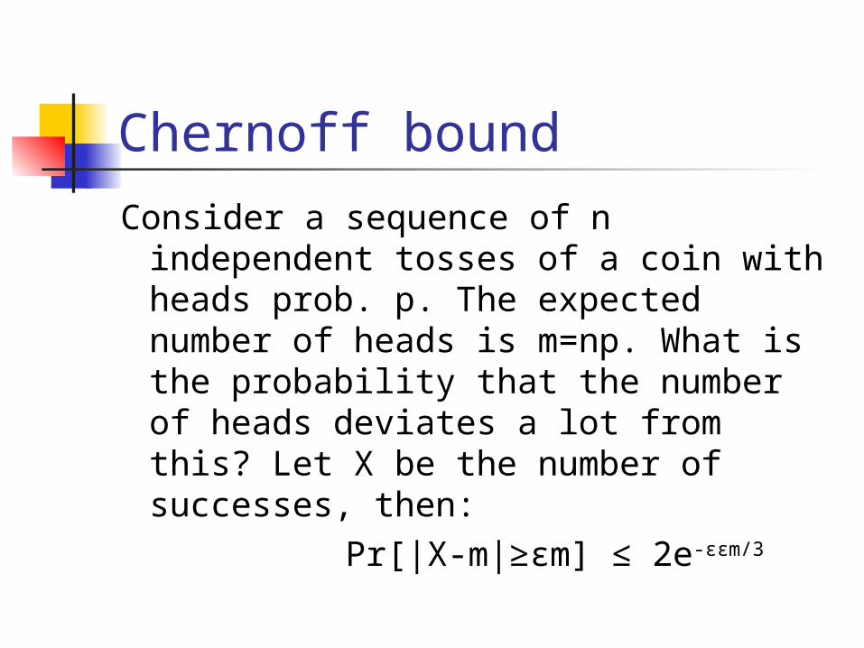
Chernoff bound

Consider a sequence of n independent tosses of a coin with heads prob. p. The expected number of heads is m=np. What is the probability that the number of heads deviates a lot from this? Let X be the number of successes, then:

Pr[|X-m|≥εm] ≤ 2e-εεm/3

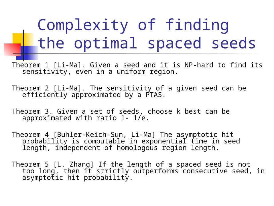
Complexity of finding the optimal spaced seeds

Theorem 1 [Li-Ma]. Given a seed and it is NP-hard to find its sensitivity, even in a uniform region.

Theorem 2 [Li-Ma]. The sensitivity of a given seed can be efficiently approximated by a PTAS.

Theorem 3. Given a set of seeds, choose k best can be approximated with ratio 1- 1/e.

Theorem 4 [Buhler-Keich-Sun, Li-Ma] The asymptotic hit probability is computable in exponential time in seed length, independent of homologous region length.

Theorem 5 [L. Zhang] If the length of a spaced seed is not too long, then it strictly outperforms consecutive seed, in asymptotic hit probability.

5. Applications beyond bioinformatics

Stock Market PredictionZou-Deng-Li: Detecting Market Trends by Ignoring It, Some Days, March, 2005

A real gold mine: 4.6 billion dollars are traded at NYSE daily.

Buy low, sell high. Best thing: God tells us market trend Next best thing: A good market indicator.

Essentially, a “buy” indicator must be: Sensitive when the market rises Insensitive otherwise.

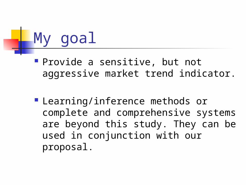
My goal Provide a sensitive, but not

aggressive market trend indicator.

Learning/inference methods or complete and comprehensive systems are beyond this study. They can be used in conjunction with our proposal.

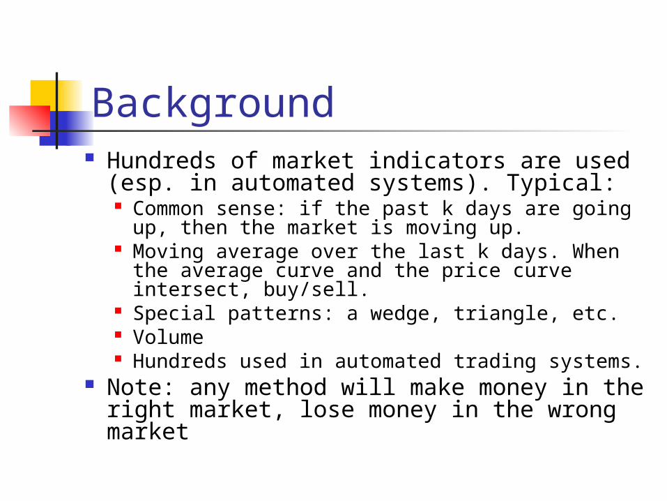
Background Hundreds of market indicators are used

(esp. in automated systems). Typical: Common sense: if the past k days are going up,

then the market is moving up. Moving average over the last k days. When the

average curve and the price curve intersect, buy/sell.

Special patterns: a wedge, triangle, etc. Volume Hundreds used in automated trading systems.

Note: any method will make money in the right market, lose money in the wrong market

Problem Formalization The market movement is modeled as a 0-1 sequence, one bit

per day, with 0 meaning market going down, and 1 up. S(n,p) is an n day iid sequence where each bit has probability

p being 1 and 1-p being 0. If p>0.5, it is an up market Ik=1k is an indicator that the past k days are 1’s.

I8 has sensitivity 0.397 in S(30,0.7), too conservative I8 has false positive rate 0.0043 in S(100, 0.3). Good

Iij is an indicator that there are i 1’s in last j days. I811 has high sensitivity 0.96 in S(30,0.7) But it is too aggressive at 0.139 false positive rate in S(100, 0.3).

Spaced seeds 1111*1*1111 and 11*11111*11 combine to have sensitivity 0.49 in S(30,0.7) False positive rate 0.0032 in S(100, 0.3).

Consider a betting game: A player bets a number k. He wins k dollars for a correct prediction and o.w. loses k dollars. We say an indicator A is better than B, A>B, if A always wins more and loses less.

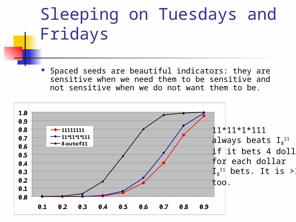
Sleeping on Tuesdays and Fridays

Spaced seeds are beautiful indicators: they are sensitive when we need them to be sensitive and not sensitive when we do not want them to be.

0.00.10.20.30.40.50.60.70.80.91.0

0.1 0.2 0.3 0.4 0.5 0.6 0.7 0.8 0.9

1111111111*11*1*1118-out-of-11

11*11*1*111always beats I8

11

if it bets 4 dollarsfor each dollar I8

11 bets. It is >I8 too.

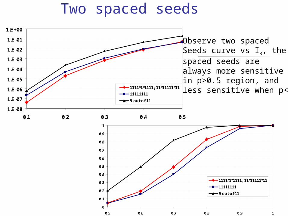
Two spaced seeds

1.E-08

1.E-07

1.E-06

1.E-05

1.E-04

1.E-03

1.E-02

1.E-01

1.E+00

0.1 0.2 0.3 0.4 0.5

1111*1*1111; 11*11111*11

11111111

9-out-of-11

0

0.1

0.2

0.3

0.4

0.5

0.6

0.7

0.8

0.9

1

0.5 0.6 0.7 0.8 0.9 1

1111*1*1111; 11*11111*11

11111111

9-out-of-11

Observe two spaced Seeds curve vs I8, thespaced seeds arealways more sensitivein p>0.5 region, andless sensitive when p<0.5

Two experiments We performed two trading

experiments One artificial One on real data (S&P 500, Nasdaq

indices)

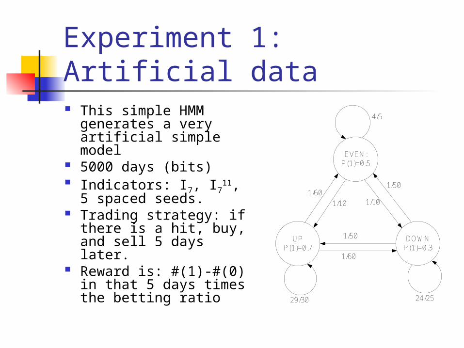
Experiment 1: Artificial data This simple HMM

generates a very artificial simple model

5000 days (bits) Indicators: I7, I711, 5

spaced seeds. Trading strategy: if

there is a hit, buy, and sell 5 days later.

Reward is: #(1)-#(0) in that 5 days times the betting ratio

EVEN:P(1)=0.5

UPP(1)=0.7

DOWNP(1)=0.3

4/5

1/10 1/10

24/25

1/50

1/50

29/30

1/60

1/60

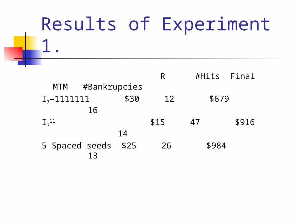
Results of Experiment 1.

R #Hits Final MTM #Bankrupcies

I7=1111111 $30 12 $679 16

I711 $15 47 $916 14

5 Spaced seeds $25 26 $984 13

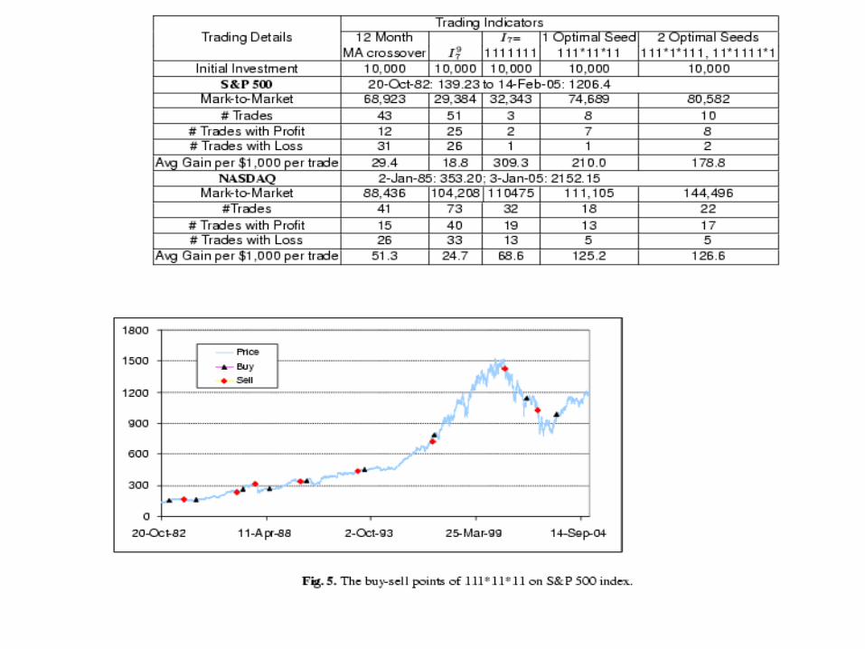
Experiment 2. Historical data of S&P 500, from Oct 20, 1982 to

Feb. 14, 2005 and NASDAQ, from Jan 2, ’85 to Jan 3, 2005 were downloaded from Yahoo.com.

Each strategy starts with $10,000 USD. If an indicator matches, use all the money to buy/sell.

While in no ways this experiment says anything affirmatively, it does suggest that spaced patterns can serve a promising basis for a useful indicator, together with other parameters such as trade volume, natural events, politics, psychology.

Open QuestionsI have presented a simple idea of optimized spaced seeds

and its applications in homology search and time series prediction.

Open questions & current research: Complexity of finding (near) optimal seed, in a uniform

region. Note that this is not an NP-hard question. Tighter bounds on why spaced seeds are better. Applications to other areas. Apparently, the same idea

works for any time series. Model financial data Can we use varying patterns instead of one seed? When

patterns vary at the same weight, we still have same number of expected hits. However, can this increase sensitivity? One seed is just a special case of this.

Acknowledgement

PH is joint work with B. Ma and J. Tromp PH II is joint work with Ma, Kisman, and

Tromp Some joint theoretical work with Ma, Keich,

Tromp, Xu, Brown, Zhang. Financial market prediction: J. Zou, X. Deng Financial support: Bioinformatics Solutions

Inc, NSERC, Killam Fellowship, CRC chair program, City University of Hong Kong.

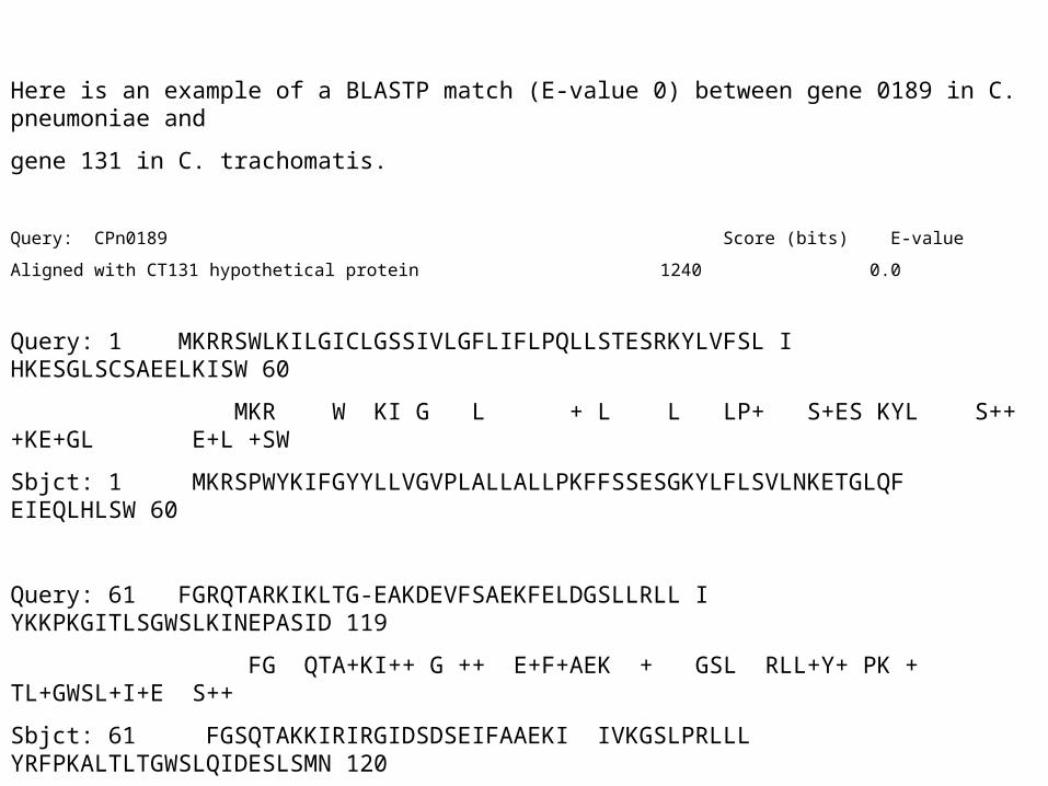
Here is an example of a BLASTP match (E-value 0) between gene 0189 in C. pneumoniae and

gene 131 in C. trachomatis.

Query: CPn0189 Score (bits) E-value

Aligned with CT131 hypothetical protein 1240 0.0

Query: 1 MKRRSWLKILGICLGSSIVLGFLIFLPQLLSTESRKYLVFSL I HKESGLSCSAEELKISW 60

MKR W KI G L + L L LP+ S+ES KYL S+++KE+GL E+L +SW

Sbjct: 1 MKRSPWYKIFGYYLLVGVPLALLALLPKFFSSESGKYLFLSVLNKETGLQF EIEQLHLSW 60

Query: 61 FGRQTARKIKLTG-EAKDEVFSAEKFELDGSLLRLL I YKKPKGITLSGWSLKINEPASID 119

FG QTA+KI++ G ++ E+F+AEK + GSL RLL+Y+ PK + TL+GWSL+I+E S++

Sbjct: 61 FGSQTAKKIRIRGIDSDSEIFAAEKI IVKGSLPRLLL YRFPKALTLTGWSLQIDESLSMN 120

Etc.

Note: Because of powerpoint character alignment problems, I inserted some white space to make it look more aligned.

Summary and Open Questions

Simple ideas: 0 created SW, 1 created Blast. 1 & 0 created PatternHunter.

Good spaced seeds help to improve sensitivity and reduce irrelevant hit.

Multiple spaced seeds allow us to improve sensitivity to approach Smith-Waterman, not possible with BLAST.

Computing spaced seeds by DP, while it is NP hard. Proper data models help to improve design of spaced

seeds (HMM) Open Problems: (a) A mathematical theory of spaced

seeds. I.e. quantitative statements for Theorem 1. (b) Applications to other fields.

Smaller (more solvable) questions: (perhaps good for course projects)

Multiple protein seeds for Smith-Waterman sensitivity?

Applications in other fields, like internet document search?

Prove Theorem 1 for other models – for example, M(3) model 0.8,0.8,0.5 together with specialized seeds.

More extensive study of Problem 3.