mimo modelling and design for mhd modes...

1MHD Workshop – New York 19/11/2007

MIMO MODELLING AND DESIGN FOR MHD MODES CONTROL IN RFX-MOD

A. Soppelsa and G.Marchiori

Consorzio RFX

Associazione EURATOM-ENEA sulla FusioneCorso Stati Uniti, 4 - 35127 Padova - Italy


OUTLINE

•Overview of the MHD active control system modelling in RFX-mod

Dynamic model of the active coils system

Dynamic model of the coil-sensor couplings

•Experimental determination of model parameters

Model validation results

•Design of a MIMO dynamic decoupler

Singular Values Decomposition analysis of the coil-sensor dynamic model

Design of the dynamic decoupler

Simulation results

•Conclusions


• L is the model of the active saddle coil system

• M is the model of the coupling between active coils and sensors

Synthetic Block Diagram of the Model Control Loop


Since the coils are mounted on two overlapping conducting structures the coupling and the dissipative parameters depend on the frequency.

Experimental data to compute the coupling terms between active coils and between active coils and sensors were collected at frequency f=w/2p=[10, 20, 50, 100, 200] Hz.

To investigate on non-axisymmetric effects due to the load-assembly, data were collected in sections of the torus both with and without special features (structure poloidal gaps,

shell poloidal gap with overlapped edges).

Experimental data acquisition for system characterization


• Overlapped gap zone (red): 86.25°<=φ<= 138.75°

• Structure 2nd gap zone (green): 273.75°<=φ<=303.75°

• First “standard” zone (blue): 183.75°<=φ<=213.75°

• Second “standard” zone (pink): φ=22.5°

Experimental data acquisition for system characterization


OUTLINE









Simulation results

•Conclusions


Computation of active coil model parameters

Self inductance and resistance of coil (26,2); mutual inductance and mutual resistance of the same coil with the adjacent ones.

10-2

10-1

100

101

102

103

-2

0

2

4

6

Indu

ctan

ce [m

H]

10-2

10-1

100

101

102

103

0

0.5

1

1.5

2

Frequency [Hz]

Resis

tanc

e [ Ω

]

( 0, 0)( 0, 1)( 0,-1)( 1, 0)(-1, 0)

• The “off-diagonal” dissipative terms are associated only to the passive structures, which react to the currents induced in the surrounding active coils, as well.

• The coupling terms are singled out by a couple of numbers, where the digits 0 e ±1 mean invariance and increment/decrement along the toroidal (first digit of the couple) and poloidal (second digit of the couple) direction.

• The relative weight of self and mutual inductance is apparent and, in particular, the greater importance of the coupling with the toroidally adjacent coils, consistently with the longer length of the poloidal leg, can be appreciated.


OUTLINE









Simulation results

•Conclusions


Computation of active coil-sensor couplings

1 0- 2

1 0- 1

1 00

1 01

1 02

1 03

- 1 3 0

- 1 2 0

- 1 1 0

- 1 0 0

- 9 0

Am

plit

ude

[dB

]

1 0- 2

1 0- 1

1 00

1 01

1 02

1 03

- 1 5 0

- 1 0 0

- 5 0

0

F r e q u e n c y [ H z ]

Pha

se [

°]

( 2 6 , 1 )( 2 6 , 2 )( 2 6 , 3 )( 2 6 , 4 )

Mutual coupling of the coils in the poloidal array 26 with the underlying sensor.

• At high frequency the presence of the inner equatorial gap compensates for the reduced size of the inner coil-sensor couple, the corresponding mutual inductance resulting larger than the others where the shielding of the passive structures is more effective.



Mutual coupling of the outer coils with the underlying sensors at 50 Hz

0 5 1 0 1 5 2 0 2 5 3 0 3 5 4 0 4 5 5 04

5

6

7

8

9

1 0

Am

plit

ude

[ µH]

T o r o i d a l i n d e x

• The most significant differences are near the structure and shell poloidal gaps

• (14,1) is the highest since there is no short-circuit element in the inner shell edge on its right side.

• The following three mutual inductances are the lowest, as the corresponding couples face the shell overlapped edges with the outer one regularly short-circuited.

• Lower deviations in the section of the structure second poloidal gap; the largest two terms result (38,1) and (40,1), the former couple encircling a pumping port and the latter spanning the poloidal gap.

• The average values of the “standard” zone appear at the other positions.


Evaluation of the coil-sensors transfer function matrix

1 0- 3

1 0- 2

1 0- 1

1 00

1 01

1 02

1 03

- 2 0 0

- 1 5 0

- 1 0 0n Z e r o s = 1 , n P o l e s = 3 ; C o u p l i n g ( 1 7 , 1 ) - ( 1 6 , 2 )

Am

plit

ude

[dB

]

1 0- 3

1 0- 2

1 0- 1

1 00

1 01

1 02

1 03

0

5 0

1 0 0

1 5 0

2 0 0

Pha

se [

Deg

]

F r e q u e n c y [ H z ]

Frequency response relative to the coupling between coil (16, 2) and sensor (17, 1). Model (blue point),

measured (red circle).

• Automatic evaluation of the coil-sensor transfer functions. It is based on a MATLAB toolbox routine providing the numerator and denominator coefficients of the transfer function which best fits in a least square sense an assigned set of experimental frequency response data. According to the couple coil-sensor, a different number of zeros and poles of the transfer functions was necessary to achieve the best fitting.

• In order to achieve a satisfactory agreement in reproducing the time evolution of the magnetic flux as many as 52 coil-sensor mutual inductances were considered in the final version (reaching a number of about 6000 states). The dynamic and steady state errors are generally about 5%, which was assessed sufficient for the design and performance analysis of an active control system of MHD modes.


T o r o i d a l n u m b e r

Pol

oida

l num

ber

L o g a r i t h m i c n o r m a l i s e d m a g n i t u t e [ l o g 1 0 ( a b s ( M ) / m a x ( m a x ( a b s ( M ) ) ) ] a t 2 0 [ H z ]

5 1 0 1 5 2 0 2 5 3 0 3 5 4 0 4 5

0 . 5

1

1 . 5

2

2 . 5

3

3 . 5

4

4 . 5

- 5

- 4 . 5

- 4

- 3 . 5

- 3

- 2 . 5

- 2

- 1 . 5

- 1

- 0 . 5

0• It is worth while noticing how

far the effect of a coil can propagate to less shielded sensors. In the figure the case of sensor (14,1) and sensors spanning the toroidal inner gap are shown.

• Each sensor measure is clearly affected by many “small” (~1% of the overlying coil) contributions.

• They add up with the same sign for coil current distributions with low m and n.



T o r o i d a l n u m b e r

Pol

oida

l num

ber

L o g a r i t h m i c n o r m a l i s e d m a g n i t u t e [ l o g 1 0 ( a b s ( M ) / m a x ( m a x ( a b s ( M ) ) ) ] a t 2 0 0 [ H z ]

5 1 0 1 5 2 0 2 5 3 0 3 5 4 0 4 5

0 . 5

1

1 . 5

2

2 . 5

3

3 . 5

4

4 . 5

- 4

- 3 . 5

- 3

- 2 . 5

- 2

- 1 . 5

- 1

- 0 . 5

0• Another example is given

for shot 22470.

• The coil (38,3) was fed at 200 Hz. The same effect of the anomalous position (14,1) is visible notwithstanding the lower signal to noise ratio and the distance.



Considerations for the dynamic model implementation

• The active coil parameters (inductances and resistances) exhibit a much lower dependence on the frequency than the mutual couplings between the active coils and the sensors.

• A constant matrix representation for the active coils parameters could then be chosen, while the full transfer function matrix was needed to reproduce the behaviour of the coil-sensor couplings. A more convenient and numerically robust state representation was then derived and used to build the MIMO model.


OUTLINE









Simulation results

•Conclusions


Experimental validation: active coil model

0 0 . 1 0 . 2 0 . 3- 4 0

- 2 0

0

2 0

4 0

C o i l ( 4 6 , 1 )

Cur

rent

[A

]

0 0 . 1 0 . 2 0 . 3- 2 0

0

2 0

4 0

6 0

8 0

C o i l ( 4 6 , 2 )

0 0 . 1 0 . 2 0 . 3

- 6 0

- 4 0- 2 0

0

2 04 0

C o i l ( 1 4 , 3 )

T i m e [ s ]

Cur

rent

[A

]

0 0 . 1 0 . 2 0 . 3- 8 0- 6 0

- 4 0

- 2 0

02 0

4 0C o i l ( 1 4 , 4 )

T i m e [ s ]

• In the presented case (Shot #17523: a 10 Hz rotating field imposed in a plasma shot with virtual shell) the 10 Hz values of inductance and resistance were used to make up the matrices. The agreement is satisfactory confirming that the number of 5 coupling terms between active coils is sufficient and that it is an acceptable assumption to neglect the coupling between plasma and active coil currents.

Comparison between model (blue dashed) and measured (red) saddle coil currents in a shot with plasma.


Experimental validation: active coil-sensor model

•Tests executed applying the measured coil currents as system inputs and evaluating the radial components of the magnetic field as model outputs.

• In the figure fluxes measured in shot #17136 (m=1, n=2 mode) by 4 poloidal arrays of saddle probes are compared with the corresponding model outputs.

•Similar successful validation procedures have been carried out in order to test the model in virtual shell closed loop operation.

0 0 . 1 0 . 2 0 . 3

- 2

0

2

Flu

x [m

Wb]

( 2 6 , 1 )

0 0 . 1 0 . 2 0 . 3

- 2

0

2( 2 6 , 2 )

0 0 . 1 0 . 2 0 . 3

- 2

0

2

Flu

x [m

Wb]

( 2 6 , 3 )

0 0 . 1 0 . 2 0 . 3

- 2

0

2( 2 6 , 4 )

0 0 . 1 0 . 2 0 . 3

- 2

0

2

Flu

x [m

Wb]

( 4 0 , 1 )

0 0 . 1 0 . 2 0 . 3

- 2

0

2( 4 0 , 2 )

0 0 . 1 0 . 2 0 . 3

- 2

0

2

Flu

x [m

Wb]

T i m e [ s ]

( 4 0 , 3 )

0 0 . 1 0 . 2 0 . 3

- 2

0

2

T i m e [ s ]

( 4 0 , 4 )


OUTLINE









Simulation results

•Conclusions


SVD Analysis of the model of the coil-sensor couplings

•The input and output singular vectors can be interpreted as coil current and flux distributions, respectively.

•The Singular Values give a measure of the system effectiveness in creating different magnetic flux distributions.

•Since the input and output singular vectors are very close in the case of RFX-mod, only the input ones are shown in the following figures.



•An example of the most effective distribution is given in the figure.

• It consists in feeding the outer toroidal array with alternate sign and it does not correspond to any modal distribution.

•The SVD analysis results to be a useful tool to get an insight into the physical properties and limits of the system.



• Two more examples of distributions are here presented to highlight the effect of neglecting small coupling terms in calculating the svd decomposition.

• In this case the most ineffective one is shown: it is very close to a m=0, n=1 modal distribution.



• The figure shows the increasing effect of the toroidal disuniformity in making a distribution ineffective at increasing frequency. A distribution aimed at keeping the flux at zero along the equatorial gap and in the region near the sensor (14,1) is ranked in the lowest positions.


OUTLINE









Simulation results

•Conclusions


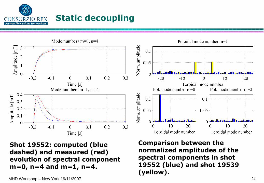
Static decoupling

Shot 19552: computed (blue dashed) and measured (red) evolution of spectral component m=0, n=4 and m=1, n=4.

Comparison between the normalized amplitudes of the spectral components in shot 19552 (blue) and shot 19539 (yellow).


Dynamic Decoupling

• The decoupler W has been calculated through a pseudo-inversion of the model M instead of a standard inversion because the last singular value is ideally equal to zero.

• This is a consequence of having a set of sensors exactly covering a closed surface.

[ ] [ ]

)j(U)j()j(V)j(W

)j(v)j(V)j(0

0)j()j(u)j(U)jω(M

H1

H192

192192

ωωωω

ωωωσ

ωωω

−Σ=

Σ=


OUTLINE









Simulation results

•Conclusions


Dynamic Decoupling

• Simulations of mode tracking and mode rejection: a comparison between a controller with dynamic decoupler and now operating, SISO approach designed, PI regulator


Dynamic Decoupling


OUTLINE









Simulation results

•Conclusions


CONCLUSIONS

• A MIMO full electromagnetic dynamic model of the MHD mode control active control system has been derived starting from the experimental data

• SVD analysis turned out to be a useful tool to gain insight on the system properties and limits

• A MIMO dynamic decoupler has been designed on the basis of the model

Simulations show promising results in terms of system tracking and rejection capability

Implementation activity started and experimental tests are foreseen in the next year

mimo modelling and design for mhd modes...

Documents