mimo configurable array for sector/omni-directional...
TRANSCRIPT

MIMO configurable array forsector/omni-directional coverage
KONSTANTINOS PRIONIDIS
Department of Signals & Systems
Chalmers University of Technology
Gothenburg, Sweden 2014


Abstract
A reconfigurable multiport antenna intended for base station use is designed and aprototype is manufactured. The antenna is composed of twelve elements; eight monopole-patches which provide vertical polarization and four loops acting as magnetic dipolesproviding horizontal polarization. The antenna can operate under various configurations,namely as a twelve, eight (logical) or two (logical) port antenna. In particular, when intwo-port mode, the antenna has two logical ports, one for each orthogonal polarizationand in addition can act as either an omni-directional or a sector-beam radiator, henceproviding extra usability. Apart from traditional measurements (S-parameters, radiationpatterns etc.) the antenna is also characterized in terms of diversity gain and MIMOcapacity by measurements in a reverberation chamber. Furthermore, simulations inHuawei’s channel emulator are performed in order to be investigated whether differentantenna patterns give different performance in various space distributions of mobile users.


Acknowledgements
Foremost, i would like to thank my principal supervisor, Mattias Gustafsson, for givingme the opportunity to work in such an exciting project and for his constant scientificconsultation. Mattias believed in me and this is of great importance to me. Addition-ally, i would like to thank Mats Hogberg and Bengt Madeberg who willingly helped mewhenever asked, without any second thoughts as well as my academic supervisor, Dr.Xiaoming Chen, and Prof. Per-Simon Kildal for their useful comments and remarks.I would also like to thank ”Bluetest AB” and John Kvarnstrand for giving me access totheir reverberation chambers and Dr. Tilmann Wittig from ”CST Computer SimulationTechnology AG” for the interest he showed in this project and his eagerness to assist me.
My gratitude towards my family is just indescribable.
Konstantinos Prionidis, Goteborg 22/08/2014


Contents
1 Introduction 1
2 Background 2
2.1 Antenna . . . . . . . . . . . . . . . . . . . . . . . . . . . . . . . . . . . . . 22.2 Wave and Antenna Polarization . . . . . . . . . . . . . . . . . . . . . . . . 32.3 Antenna arrays, beamforming and coupling . . . . . . . . . . . . . . . . . 52.4 Diversity and MIMO . . . . . . . . . . . . . . . . . . . . . . . . . . . . . . 10
3 Antenna Design 16
3.1 Half-wavelength Dipole Antenna . . . . . . . . . . . . . . . . . . . . . . . 183.2 Horizontal Polarized Element . . . . . . . . . . . . . . . . . . . . . . . . . 203.3 Horizontally polarized Array . . . . . . . . . . . . . . . . . . . . . . . . . 243.4 Vertical Polarized Element . . . . . . . . . . . . . . . . . . . . . . . . . . . 263.5 Dual Polarized Antenna . . . . . . . . . . . . . . . . . . . . . . . . . . . . 293.6 Prototype . . . . . . . . . . . . . . . . . . . . . . . . . . . . . . . . . . . . 31
4 Diversity and MIMO 35
4.1 Antenna diversity simulations . . . . . . . . . . . . . . . . . . . . . . . . . 364.2 Reverberation Chamber . . . . . . . . . . . . . . . . . . . . . . . . . . . . 384.3 Channel Simulations . . . . . . . . . . . . . . . . . . . . . . . . . . . . . . 40
5 Conclusions and Future work 42
5.1 Conclusions . . . . . . . . . . . . . . . . . . . . . . . . . . . . . . . . . . . 425.2 Future work . . . . . . . . . . . . . . . . . . . . . . . . . . . . . . . . . . . 43
Bibliography 46
A Mathematical expressions for radiating fields 47
B Antenna Structure figures 50
i

CONTENTS
C Reverberation Chamber and channel simulation 58
D Return Loss and coupling 64
E Radiation Patterns 72
F HFSS vs CST studio suite 85
ii

1Introduction
Increasing number of mobile users and the ever growing demand for data traffic requirethe redesign of existing mobile networks in order to become more efficient and providehigher capacity. Reduction of inter-cell interference which will increase the networkspectral efficiency and the need of better power efficiency tend to decrease the size ofthe cells (micro-cells, pico-cells) and as a result new types of base stations with smartantennas that can adapt to different environments and exploit the possibilities of amultipath environment should be employed.
The purpose of this master thesis is the development of such a smart base stationantenna which can support MIMO and yet having the ability to adapt in various envi-ronments by having a flexible radiation pattern. The driving idea is that the antennato be designed consists of two independent orthogonal polarized antenna arrays whichin principle radiate omni-directionally but also have the ability to form sector beamsby proper phase excitation of each individual element. In this way, for instance, theantenna could be used as an omni-directional radiator when placed in the center of acity square or as a sector radiator when facing a street or mounted on a wall while, atthe same time, having the ability to transmit/receive distinct information through twouncorrelated streams; one through each orthogonal polarization. Moreover, since theantenna will be formed by many elements, it could be used in a higher order MIMO torapidly increase the point-to-point capacity.
In this report, the background theory that supports the concept of the antenna isinitially given in chapter 2. Chapter 3 describes the whole process of the antenna de-velopment together with simulated and measured results. In chapter 4, the antenna ischaracterized in respect to diversity and MIMO capabilities and its performance is in-vestigated through network simulations whilst Chapter 5 contains a brief conclusion andsuggestions for further investigation. Finally, in appendix F, a performance comparisonbetween two commercial 3D-EM simulation softwares is discussed.
1

2Background
2.1 Antenna
An antenna is a device which can either receive or transmit electromagnetic energy.Antennas are essential components of wireless communication systems since it is thosethat will transform the information produced in a transmitter to electromagnetic wavesthat can travel through the air or, the inverse way, it is the component that will receiveelectromagnetic waves and guide them to the receiver where the information can bedecoded.
An antenna can be as simple as a piece of cable where acceleration of flowing chargedue to bending, termination or in general due to discontinuities will result in electro-magnetic radiation [1, p. 9]. But antennas can also be complex and very big structures.In traditional Line of Sight (LOS) environments, antennas are characterized mainly bytheir radiation pattern and the radiation efficiency. The radiation pattern (radiationfields or far field function) describes how the antenna directs the energy that is acceptedin its ports, towards free space. The ideal case is an isotropic antenna which spreads theelectromagnetic energy equally in space (figure 2.1(a)), thus having a power gain of 1throughout the whole sphere. Another kind of radiation pattern which is commonly seenin practice is the so called omni-directional pattern (figure 2.1(b)) and is considered theclosest possible realistic equivalent of isotropic radiation. The omni-directional pattern,has a power gain larger than one at elevation angle θ = 90o but almost zero at θ = 0o
and is the best choice of antenna if we demand the widest possible coverage. Amongmany others, there is also the sector beam pattern (figure 2.1(c)). An antenna with asector beam pattern radiates most of the energy towards a particular direction, a veryuseful feature, hence it is widely used in today’s wireless communications.
The radiation efficiency of an antenna is a metric of how well the antenna radiatesthe power that has been accepted by the antenna port. Said in another way, radiation ef-ficiency represents the ohmic losses of the antenna, that is the energy that is absorbed by
2

2.2. Wave and Antenna Polarization CHAPTER 2. Background
(a) Isotropic pattern (b) Omni pattern (c) Sector Beam
Figure 2.1: Examples of radiation patterns
the antenna and not radiated. It is the ratio of the power radiated to the power accepted :
erad =Prad
Pacc
where :
• Prad is the radiated power
• Pacc is the accepted power
One can also include more factors of efficiency such as transmission efficiency, er,which accounts for the mismatch losses and polarization efficiency epol (see section 2.2)to calculate a total antenna efficiency [2, p. 50] :
eant = erad · er · epol
2.2 Wave and Antenna Polarization
The electromagnetic (EM) fields that are radiated by an antenna are usually producedby steady sinusoidal sources hence the fields will have steady sinusoidal time variationas well, thus the instantaneous field at any point can be written as :
−→E (x,y,z,t) = ReE(x,y,z)ejωt and
−→H (x,y,z,t) = ReH(x,y,z)ejωt
for the electric and magnetic field respectively. Each vector field have both x, y and z
but in the far field1 the longitudinal field component z becomes negligible and the field
1The far field of the antenna is at a distance ≥ D2/λ (D is the largest dimension of the antenna)fromthe phase center and it is the region where the radiation pattern is measured. This condition is calledFraunhofer condition.
3

2.2. Wave and Antenna Polarization CHAPTER 2. Background
(a) Linear x-polarized (ver-tical)
(b) Linear y-polarized (hor-izontal)
(c) Linear Polarized at 45o
angle
Figure 2.2: Examples of linear polarized waves. The wave propagates towards the readerand the red line represents the electric field vector
can be considered quasi-TEM field [3, p. 90]. This means that if the radiated wave ispropagating towards the z-axis then both the electric and magnetic field lie on the x-yplane, i.e perpendicular to the direction of propagation and on a right angle betweenthem. Hence, the electric field can be written as :
E = [Exx+ Eyy]e−jkz, where:
Ex : is the x-component of the electric fieldEy : is the y-component of the electric fieldk : is the wave number ( k = 2π/λ) .
The polarization of a plane wave is defined as the direction of its electric field. A wavecan be linear, circular or in general, elliptical polarized. If the electric field is directedon a fixed line in the x-y plane for any distance z, then we say that the field is linearlypolarized. If this line is the x-axis or y-axis then the wave is x-polarized or y-polarizedrespectively but in general it can be linear polarized at any angle in-between (see figure2.2). When spherical coordinates are used instead, then we can say that the wave is θor φ polarized (figure 2.3). In practice the terms vertical and horizontal polarization(relative to the direction of propagation) are commonly used and this is the notationthat will mainly be used in this report.
In order for the field to be linear polarized the phase difference between the x andy component should be k × π for k:integer. If the two components are equal and theyhave a phase difference of |π/2| then the wave is circular polarized. In any other case thepolarization is elliptical. It is the concept of the two orthogonal polarizations, verticaland horizontal, that this project is partly based upon so here we don’t go into moredetails regarding circular and elliptical polarizations.
A transmitting antenna’s polarization depends on the polarization of the wave thatit generates. For instance, if the waves going out of an antenna are linearly, verticalpolarized then we say that the antenna is vertical polarized. Due to reciprocity, the
4

2.3. Antenna arrays, beamforming and coupling CHAPTER 2. Background
Figure 2.3: Field vector and components in spherical coordinates.
same holds for a receiving antenna, that is, a receiving antenna can get the most out ofan incident wave (in terms of power) if its polarization is the same as that of the incidentwave, i.e they are aligned.
2.3 Antenna arrays, beamforming and coupling
(a) Linear array (b) Planar array
Figure 2.4: Example of array types. A linear, N elements array to the left and an NxMplanar array to the right.
Individual antenna elements, such as simple electric dipoles for example, can becombined together to form a collection called array which can provide, in general, higherdirectivity values. Moreover, they give flexibility regarding the radiation pattern sinceit is possible to shape it by changing the amplitude, position or the phase excitation ofthe individual elements. Arrays are called linear when the elements are positioned along
5

2.3. Antenna arrays, beamforming and coupling CHAPTER 2. Background
one direction, x, y or z (figure 2.4(a)) and planar when positioned along two directions,xy or xz for instance (figure 2.4(b)).
To show the operation of an antenna array we will consider the simplest case of auniform, linear, 2-element array in a 2-D environment. It is called uniform because theelements are identical and equally spaced with the same amplitude and a progressivephase change, although in general an array can be formed by elements of any type, withnon uniform amplitude, phase or spacing.
Figure 2.5: Two element linear array.
Consider the observation pointOP and the elements 1 and 2 that are positioned alongthe axis in a distance d (figure 2.5). If we neglect any coupling effect (see later), sincethe elements are identical they will have the same radiation patterns,G(r) or G(r,θ,φ).Hence, by referring to each element’s individual reference point (let’s say the center ofeach element), the electric field at OP will be :
E1 = 1r1e−j(k·r1+p1)G(r1), due to element 1
and
E2 = 1r2e−j(k·r2+p2)G(r2), due to element 2
where r1 and r2 are the distance from element 1 and 2 to the OP respectively, 1r is
the divergence factor, namely how the amplitude attenuates with distance and p1, p2 arethe phase excitations of each element. Since superposition holds, the total field at OP
will be :
E = E1 +E2 =1
r1e−j(k·r1+p1)G(r1) +
1
r2e−j(k·r2+p2)G(r2). (2.1)
6

2.3. Antenna arrays, beamforming and coupling CHAPTER 2. Background
Moreover, if the OP is located far enough, we can use the Fraunhofer approximations,that is :
1. 1r1
≃ 1r2
≃ 1r
2. θ1 ≃ θ2 ≃ θ
3. r1 = |r− dx| = r − dx · r = r − dx · cos(θ1) ≃ r − dx · cos(θ) = r − d2 · cos(θ)
4. r2 = |r+ dx| = r + dx · r = r + dx · cos(θ2) ≃ r + dx · cos(θ) = r + d2 · cos(θ)
where 1 holds for amplitude and 3,4 for phase variations. Hence the total field at OP
becomes :
E =1
re−j(k(r−d·cos(θ)/2)−dp/2)G(r) +
1
re−j(k(r+d·cos(θ)/2)+dp/2)G(r)
=1
re−j(k·r−k·d·cos(θ)/2−dp/2)G(r) +
1
re−j(k·r+k·d·cos(θ)/2+dp/2)G(r)
=1
r·G(r) · e−jk·r[ej(k·d cos(θ)+dp)/2 + e−j(k·d cos(θ)+dp)/2]
=1
r·G(r) · e−jk·r · 2 cos(1
2(k · d · cos(θ)) + dp) (2.2)
where dp is the phase difference between the elements and since it is progressive, p1and p2 are substituted by −dp/2 and +dp/2 respectively. In addition, G(r1) and G(r2)are substituted by G(r) because of approximation condition (2). In last line of equa-tion 2.2 Euler’s equation has been used.
Equation 2.2 can be divided in two parts. The first one, 1r · G(r) · e−jk·r can be
recognized as the element’s contribution to the electric field at OP with the referencepoint lying in the center of the axis. The second part,
2 cos(1
2(k · d · cos(θ)) + dp) (2.3)
is called Array Factor and it is the contribution of the individual elements’ combination.From equation 2.3 it is obvious now that changing the spacing d or the phase p of theelements we alter the array factor and hence the total radiation pattern of the arraywill change. This technique is called beamforming and conceptually is based on thefact that waves radiated by different elements combine sometimes constructively andothers destructively thus forming a particular radiation pattern in space. If identicalelements are used in the array, with similar amplitudes and fixed positions, then theirindividual phase can be used to shape the radiation pattern either by analog phase shiftercomponents or in baseband. This type of arrays are called phased arrays and is one ofthe principles this project is based upon.
7

2.3. Antenna arrays, beamforming and coupling CHAPTER 2. Background
By observing equation 2.2 and considering that identical elements are used in thearray one can conclude that each element can be replaced by a point source, then thearray factor can be calculated considering the point sources and in the end multiply withthe elements’ radiation pattern to get the array’s radiation pattern. Each point sourcecan have the amplitude, position and phase excitation of the element that it replaces.With this in mind we can generalize the array factor for N elements, linearly positionedalong one axis. Referring to figure 2.6 and assuming the phase of the first element iszero, the array factor for N elements can be written as :
AFlin = α11 + α2ej(kd2 cos(θ)+p2) + α3e
j2(kd3 cos(θ)+p3) + · · ·+ αNej(N−1)(kdN cos(θ)+pN )
=N∑
n=1
αnej(n−1)(kdn cos(θ)+pn) (2.4)
Figure 2.6: Linear N array
Moreover, assuming that the array is uniform (uniform spacing and phase difference)with equal element amplitudes, equation 2.4 simplifies to
AFlin u = 1 + ej(kd cos(θ)+p) + ej2(kd cos(θ)+p) + · · ·+ ej(N−1)(kd cos(θ)+p)
=
N∑
n=1
ej(n−1)(kd cos(θ)+p) (2.5)
Expanding the analysis of the array factor to planar arrays (figure 2.7), we can thinkof a planar array as a linear collection (in y direction) of linear arrays (in x direction).Hence, by following the same reasoning as above the array factor of a planar array can
8

2.3. Antenna arrays, beamforming and coupling CHAPTER 2. Background
Figure 2.7: Planar NxM array
be written as :
AFpl =
M∑
m=1
AFlinβmej(m−1)ξm
=
M∑
m=1
(
N∑
n=1
αnej(n−1)ψn
)
βmej(m−1)ξm
=
(
N∑
n=1
αnej(n−1)ψn
)(
M∑
m=1
βmej(m−1)ξm
)
(2.6)
= AFlinX ·AFlinY (2.7)
thus, the array factor of a planar array is the product of the linear array factor in x-direction and the one in y direction.
In equation 2.6,
ψn = k · dxn · sin(θ) cos(φ) + pxn
and
ξm = k · dym · sin(θ) sin(φ) + pym
because when the observation point is in 3-dimension space and the elements lie on
9

2.4. Diversity and MIMO CHAPTER 2. Background
the x or y axis, the distance to the axis origin is dependent on both θ and φ angles1.That is, the distance that a wave travels with respect to the reference point dependsboth on elevation and azimuth angles.
In the preceding analysis it has been assumed that since the elements that are usedin the array are identical, their radiation patterns are exactly the same. In reality whenan individual element radiates, some of the radiated energy is absorbed by the neigh-boring elements resulting in reduction of the element’s efficiency. Moreover, part of thisabsorbed energy will be re-scattered back, radiated and absorbed by the (initially) radi-ating element, forming new currents in the antenna and eventually altering the radiationpattern and the input impedance of the element. This electromagnetic interaction be-tween radiating elements is called mutual coupling and mainly depends on the type ofthe antennas (radiation characteristics) and their relative distance.
In order to be more precise when calculating the array factor or the total radiationefficiency of an array, the embedded element pattern [4] and the embedded elementradiation efficiency should be measured. That is, the radiation pattern and the radiationefficiency of an element when all other elements of the array are present and terminatedwith their port impedances.
2.4 Diversity and MIMO
Wireless communication systems can exist in many different environments, from line-of-sight (LOS) where the transmitting and receiving antennas have only one straight pathto environments where the there are only scattered/reflected paths. LOS communicationmakes use of the traditional antenna characteristics such as the radiation pattern and inthis kind of environment the signal power decreases according to the free space model(Friis transmission equation) [5, p. 31]. On the other extreme, the transmitting andreceiving antennas can have no LOS connection but waves that have been reflected, re-fracted or scattered by objects and big obstacles may combine at the receiving antenna toprovide communication link, a phenomenon called multipath since waves follow manydifferent paths until they reach the receiving antenna. The problem with multipath en-vironments is that since the waves that arrive at the antenna are generally independentand the environment changes over time (an urban environment for instance) they maycombine sometimes constructively and others destructively giving rise to a very fast andsharp variation of the received signal power. This is called small scale fading and some-times can result in deep fade (very low received power) where communication breakdowncan occur. A comparison between free space loss and small-scale fading can be seen infigure 2.8.
In order to mitigate the effect of small scale fading and provide more robust commu-nication links diversity can be exploited. There are many kinds of diversities that canbe used such as time and frequency diversity but it’s space, radiation and polarizationdiversities that will be discussed here.
1An explanation about this is given in Appendix A and equations A.12-A.15
10

2.4. Diversity and MIMO CHAPTER 2. Background
Figure 2.8: Path Loss (red) vs Small scale fading (blue)
In space diversity more than one element can be used at the receiving antenna. Eachelement will generally sense independent signals and it is very unlikely that all signalsare in deep fade simultaneously. Thus, by combining those signals under a diversity com-bining mechanism deep fades can disappear resulting in a more robust communicationlink with increased capacity. There are several ways of combining the signals received ineach port but the three techniques used in this work are the following:
• Selection Combining (SC): The signals at each port (branch) are constantly moni-tored and always only the strongest one is forwarded to the receiver circuitry. Thisis the simplest form of signal combining and requires no complex electronics butthe diversity gain diminishes rapidly when additional branches are added.
• Equal gain Combining (EGC): The phase of the signal in each branch is correctedso that signals in all branches have the same phase and then they are all addedtogether. This is a more complex method than SC but it provides higher diversitygains.
• Maximal Ration Combining (MRC): As in EGC, phase is corrected so that signalsin all branches share the same phase. In addition, when signals are added together,each is weighted with respect to its SNR; signals with higher SNR receive moreweight. This combining technique requires the most sophisticated circuitry butproduces the highest gain among the three. MRC is also commonly know asmatched filtering.
In order for the different signals that are received to be uncorrelated, the elementsshould be spaced at least half a wavelength apart because it is known that in multipathtwo signals de-correlate approximately over a distance of half a wavelength for non-directive antenna elements. In general, the more the signals are correlated the less wegain by diversity. Diversity gains, as defined in [6], can be distinguished as apparent,effective and actual gain.
11

2.4. Diversity and MIMO CHAPTER 2. Background
Polarization and radiation pattern diversity can be understood with a similar reason-ing as above. If for instance the antenna has two ports with orthogonal polarizations (onebeing vertical polarized and the other being horizontal polarized) it will sense two differ-ent signals, one vertical and one horizontal polarized which in general, are uncorrelated.The same holds for radiation pattern diversity, namely, when the radiation patterns ofeach element do not intersect then signals sensed at each port will be independent andwill mitigate small scale fading if combined properly.
It has been mentioned before that when there are radiating elements close to eachother (in an array for instance) there will be eventually coupling among them so theradiation patterns will change and the radiation efficiency will be reduced. In diversityschemes, this has two effects. Since the embedded radiation patterns change, the signalssensed will be less correlated and this will provide some diversity gain. On the otherhand, radiation efficiency is reduced resulting in degradation of diversity gain. It has beenshown in [6] that diversity gain degradation due to reduction in radiation efficiency ishigher than improvement due to radiation pattern de-correlation so, in general, couplingbetween antenna elements will reduce the diversity gain.
It has to be noted that antenna diversity can be used at the transmitter side as well.If there is knowledge about the channel state at the transmitter then the different signalsto be transmitted can be pre-processed (with matched filtering for example) such thatthey always combine constructively at the receiver side hence deep fading is wiped out.
In transmit matched filtering, the symbol x has its phase and amplitude modifiedto match the channel to the receiver, hence it is first multiplied at the transmitter byw∗
i for i = 1 : T where T is the number of the transmit antennas. At the receiver thetransmitted signals are added up as:
y =
(
MT∑
i=1
hiw∗
i
)
x+ n = wHh x+ n (2.8)
where w is a column vector containing the complex weights w1 · · ·wT , h contain thechannel coefficients and n is white noise with zero mean and variance σ2n. If the transmitpower is denoted as P then the SNR of the received signal is:
SNR =P |wHh|2
σ2n(2.9)
The quantity |wHh|2 is maximized when the two vectors, w and h, are aligned, that iswhenw = h/||h||, thus the received signal becomes y = ||h||x+n and the post-processingSNR :
SNRMF =P ||h||2σ2n
(2.10)
Matched filtering is known to maximize the post-processing SNR.Antenna diversity schemes can also be described as single input multiple output
(SIMO) when happening at the receiver side or as multiple input single output (MISO)
12

2.4. Diversity and MIMO CHAPTER 2. Background
when happening at the transmitter side. The need for higher capacity though, gave riseto multiple input multiple output systems or MIMO where both the transmitting andthe receiving antenna have more than one element.
Figure 2.9: MT ×MR MIMO system
In a MIMO system there are MT ×MR channels formed between the MT elementsof the transmitting and the MR elements of the receiving antenna (figure 2.9). Hence, aMIMO system can be modeled as :
y(k) = H(k) ∗ x(k) + n(k) (2.11)
where :
y(k) is the MR × 1 received signal vector,x(k) is the MT × 1 transmitted signal vector,H(k) is the MR ×MT channel matrix,n(k) is the MR × 1 noise vector,
so, there are MT different signals leaving the transmitting antenna which then passthrough a multipath environment modeled by matrix H and eventually all consequentwaves combine at the MR terminals of the receiving antenna. Matrix H contains coeffi-cients for every possible link between the transmitting and receiving terminals. The noiseis Gaussian distributed with zero mean and σ2n variance and if the channel is narrow-band 2 then equation 2.11 can be written as :
y(k) = H(k)x(k) + n(k) (2.12)
If singular value decomposition is performed on matrix H, then it degenerates to :
H = UΛVH (2.13)
2When the channel is approximately constant over the whole bandwidth of the signal.
13

2.4. Diversity and MIMO CHAPTER 2. Background
Matrix Λ contains the non-negative singular values of matrix H. The number of thosepositive singular values shows how many different independent sub-channels can beformed by exploiting MIMO. Hence someone could send as many different streams ofdata through the channel as the number of positive eigenvalues of H, a process calledspatial multiplexing (SM). The number of singular values is also called the rank of matrixH and can be at most equal to min(MT ,MR).
Setting :x = VHx ⇐⇒ x = Vx (2.14)
andy = UHy ⇐⇒ y = Uy (2.15)
where x and y are the input and output data stream vectors respectively, equation 2.12can be rewritten as :
y = Hx+ n
Uy = UΛVHVx+ n
UHUy = UHUΛVHVx+UHn
y = Λx+ n (2.16)
where n = UHn has the same statistics as n. What the above equations (2.12 - 2.16)describe is that initially the data stream x is multiplied with the matrix V to get x
(pre-processing) which is then sent through the channel H while at the other end, theantenna receives y which is then multiplied with UH to recover the initial data stream(post-processing). From equation 2.16 we see that the output y is formed by the inputx enhanced by each sub-channel gain Λ plus a white Gaussian noise generated at thereceiver. The final MIMO system is presented in figure 2.10.
Figure 2.10: MT ×MR MIMO system
The capacity of a time-invariant MIMO channel is given by :
CMIMO =
rH∑
i=1
log2 (1 + SNRi) =
rH∑
i=1
log2
(
1 +P oi |λi|2σ2n
)
(2.17)
14

2.4. Diversity and MIMO CHAPTER 2. Background
where P oi is the optimal power allocated to i-th stream and |λi|2 is the gain of the i-thsub-channel. An interesting result shown in [7, p. 41] is that, by using the water-fillingoptimization algorithm, when the system operates under the high SNR regime then itis preferable to allocate equal amounts of power to all streams whilst when under lowSNR, all power should be allocated to the strongest stream (highest |λi|2). However, asit is mentioned in [8], when putting more power in the strongest stream and less to theworst one, the relative throughput of such a SVD-based MIMO system will be worsethan allocating equal amounts of power to all streams and therefore, the water-fillingtechnique is not used in practical systems such as LTE. In the same work, it is proposedan inverse power allocation scheme which is performs 2.5 dB better than the equal powerallocation and 1.5 dB better than the open-loop zero forcing MIMO system.
15

3Antenna Design
Mobile networks were formed until recently by coverage cells that are served by base sta-tions (BS) with directive antennas, usually single (vertical) polarized. The BS’s coveragecan reach up to 35 kilometers and that’s why this type of networks are called macrocellsand traditionally, macrocell architecture use relatively high amounts of power at the BSantennas in order to provide this wide coverage. Nowadays, there is the trend of scalingnetworks down in order to improve power efficiency and increase capacity so new typesof network architectures, such as microcell, picocell or even femtocell networks have beenevolved. The coverage of these cells can range from few tens of meters up to 2 kilometers,thus new types of base stations are required which in principle, are also scaled down insize and placed in a more dense way throughout urban environments.
The antenna to be developed should be a novel BS smart antenna which serves thesenew types of networks. It shall be dual polarized, that is, provide both vertical andhorizontal polarizations. In that way, since orthogonal polarizations are uncorrelatedand considering each polarization as a logical antenna port, antenna diversity and spa-tial multiplexing can be used to increase the robustness and capacity of the microwavelink. Hence, by exploiting antenna diversity, signals sensed by each polarization can getcombined together to avoid deep fades. On the other hand by making use of MIMO,two different data streams could be transmitted, one over each polarization. Of course,a prerequisite for MIMO is that the mobile device’s antenna should have more than oneelement.
In addition, the new antenna should be flexible in terms of radiation pattern so it canadapt in many different scenarios. It should for example, provide an omni-directionalpattern when placed in the middle of a city square or form a beam and direct the energywhen mounted on the wall of a building. For this reason, an array of omni-directionalelements shall be designed in order to provide both omni-directional and sector beamsby adjusting the phase of the elements in the array (beamforming).
16

CHAPTER 3. Antenna Design
It is shown later (section 3.1) that the current distribution on half-wavelength dipoleantennas is such that the antenna produces an omni-directional pattern . Electric andmagnetic dipoles can hence provide omni-directional vertical and horizontal polarizedpatterns respectively but although electric dipoles are easy to design, magnetic dipolesare in general hard to realize. On the whole, the antenna structure will be a 2x2 planararray of both electric and magnetic dipoles (figure 3.1).
Figure 3.1: A 2x2 planar array. The blue elements are electric dipoles which produce avertical polarized omni-directional pattern. The red elements are magnetic dipoles whichproduce a horizontal polarized omni-directional pattern.
As discussed in section 2.3 phase excitation of each element will determine the arrayfactor and consequently the overall radiation pattern of the array. When all elements,[1st,2nd,3rd,4th], are excited with the same phase, an omni-directional pattern is formedand the antenna is said to operate in omni mode whilst when excited with a certain phasedifference then some kind of beam shall be formed. In particular, when elements areexcited with phase vector [0o,90o,180o,90o] then a sector beam directed towards the firstelement is formed, when excited with phase vector [90o,0o,90o,180o] then a sector beamdirected towards the second element is formed and so on. In this case it is said that theantenna operates in sector mode. Another interesting beam that can be used in mobilecellular networks is created when the phase vector [0o,180o,180o,0o] is used in which casea double beam pattern is formed. The array modes are summarized in figure 3.2.
A fact to be noticed is that separation of elements in the array play a crucial roleon the array factor. As can be observed from figures E.2 and E.3 the further away theelements are positioned the more the radiation pattern is disturbed hence the elementson the array should not be placed much more than half-wavelength apart.
The three most important specifications set for the antenna to be designed are:
• Return Loss ≥ 10db between 1.7 and 2.2 Ghz 1
• Coupling ≥ 12.5 db (ideally ≥ 15db).
1Return loss is defined here as 10 log10
Pi
Prwhere Pi is the incident power and Pr is the reflected power.
17

3.1. Half-wavelength Dipole Antenna CHAPTER 3. Antenna Design
• Azimuth rippling ≤ 3db when in omni mode.
• Sidelobes shall be at least 10db lower than the main beam when in sector mode.
Moreover, the antenna shall be a compact structure and in principle cheap and easy tofabricate.
Figure 3.2: Summary of the antenna modes.
3.1 Half-wavelength Dipole Antenna
Imagine a balanced waveguide that carries a sinusoidal signal current as in figure 3.3where the end of the waveguide is connected to a dipole of length l, one line to eachdipole arm. Initially, the current wave propagates into the waveguide and then throughthe dipole until it reaches the end of the dipole arm where undergoes a total reflectionresulting in standing waves formation. As seen from the picture, these standing waveshave the same phase in both arms, hence the current distribution through the dipole 1
is given by :
I(z) =
zI0 sin[
k( l
2 − z)]
, 0 ≤ z ≤ l
2
zI0 sin[
k( l
2 + z)]
, − l
2 ≤ z ≤ 0(3.1)
As can be seen from equations A.1 and A.2 which are derived by the use of auxiliaryvector potentials [9], the electric and magnetic fields of a radiating element each has twocomponents, one due to electric and one due to magnetic surface current distribution.As there are no magnetic currents to the described dipole above (IJ 6= 0 and IM = 0),the electric field at the far-field region is described by equation A.7 and is oriented atz − (z · r)r where r is the unitary vector at the direction of propagation. Hence, theelectric field is orthogonal to the direction of propagation and vertical polarized. Said ina different way, the electric field has only a θ component since z − (z · r)r = sin(θ)θ in
1The Dipole is assumed to be positioned along the z axis. Moreover, a very thin dipole is consideredhence the current is independent of the x and y components and depends only on z.
18

3.1. Half-wavelength Dipole Antenna CHAPTER 3. Antenna Design
Figure 3.3: Current distribution in balanced waveguide and (full-wavelength) dipole. Afterreflections at both ends of the dipole, standing current waves are formed. Neighboring waveshave 180 degrees phase difference.
spherical coordinates. Consequently, the magnetic field vector lies perpendicular to theplane formed by the electric field vector and the direction of propagation.In order to find the radiating fields of the dipole, the dipole’s length is divided intoinfinitesimal parts of ∆z and then the contribution of each infinitesimal dipole is summedtogether to produce the dipole’s radiation pattern. The radiating electric field of aninfinitesimal electric dipole is known by [1], [2] as :
dEθ ≃ jηkI(z)e−jkr
4πrsin(θ)ejkz cos(θ)dz (3.2)
Using equation 3.1 in equation 3.2 and integrating over the length of the dipole, theelectric field can be written as :
Eθ ≃jkηI0e
−jkr
4πrsin(θ)
l/2∫
0
sin
[
k(l
2− z)
]
ejkz cos(θ)dz +
0∫
−l/2
sin
[
k(l
2+ z)
]
ejkz cos(θ)dz
(3.3)
which by using equation A.11 simplifies to :
Eθ ≃ jηI0e
−jkr
2πr
[
cos(
kl2 cos θ
)
− cos(
kl2
)
sinθ
]
(3.4)
For the half wavelength dipole case (l = λ/2), the current distribution on the dipole isthe one shown in figure 3.4 and equation 3.4 becomes :
Eθ ≃ jηI0e
−jkr
2πr
[
cos(
π2 cos θ
)
sinθ
]
(3.5)
and since H = 1ηz×E,
Hφ ≃ jI0e
−jkr
2πr
[
cos(
π2 cos θ
)
sinθ
]
(3.6)
19

3.2. Horizontal Polarized Element CHAPTER 3. Antenna Design
Figure 3.4: Current distribution in a half-wavelength dipole. Observe that current maxi-mum is at the middle of the dipole.
The rest of the field components, namely Eφ, Hθ and Hr are zero and Er can be alsoassumed zero for far-field observations.
From equations 3.5 and 3.6 it is apparent again that the electric field is orientedonly at the θ plane and that there is no dependence on the φ variable. So, when thecurrent going through the dipole is an electric current, the radiation pattern is omni-directional and the electric field is vertically polarized. On the other hand, if a magneticcurrent source is used instead, the radiating fields in far-field are again described byequations A.7 and A.8 with IJ = 0 and IM 6= 0 hence it is the magnetic field thatlies on the θ plane. Consequently, the electric field which is perpendicular to the planeformed by the magnetic field vector and the direction of propagation, lies on the φ planeresulting in omni-directional horizontal polarized radiation pattern.
3.2 Horizontal Polarized Element
As stated in the previous section, a short magnetic dipole can provide omni-directionalpattern and horizontal polarization. It is shown in [1] and [2] that an electrically smallloop1 with a constant current throughout the loop has the same far-field function as amagnetic dipole. However, the radiation impedance of a small loop is generally verysmall and usually smaller than the loss impedance of the wire resulting in very lowradiation efficiency, hence small loop antennas are very poor radiators and are not usedas transmitting antennas. Moreover, small loops cannot be used together with practicaltransmission lines (50 Ω or 75 Ω) because mismatch losses would be very high. Increasingthe number of turns of the loop or inserting a ferrite core of high permeability within theloop are ways to increase the radiation impedance of a small loop antenna. Increasingthe circumference of the loop is another way of increasing the radiation impedance butas the circumference increases, the current at the loop becomes non-uniform and thus
1Electrically small is considered a loop with circumference less than 0.1 λ
20

3.2. Horizontal Polarized Element CHAPTER 3. Antenna Design
the maximum radiation shifts to the axis of the loop as the circumference approachesone wavelength.
Novel horizontal polarized antennas inspired by meta-materials have been proposedin [10] and [11] but radiation efficiency and bandwidth are poor. Based on the sameconcept, innovative loop antennas that keep the current in phase throughout the loopby utilizing the artificially created infinite wavelength transmission lines are proposed in[12] and [13].
Alford and Kandoian [14] presented a way of creating an electrically large loop an-tenna which has in-phase current distribution throughout the loop hence radiating omni-directionally and horizontal polarized while having good radiation characteristics at thesame time. It is proved that having a current distribution similar to that in figure 3.5then it is possible to get a resonant loop antenna with omni-directional characteristics.Such a printed loop has been patented [15] and used again in [16] but both have a narrowbandwidth.
Figure 3.5: Alford antenna current distribution.
Referring back to figure 3.4 one can notice that such a current distribution existswhen the length of the dipole is approximately λ/2 (each of the dipole’s arm has λ/4length). Thus, by combining 4 half-wavelength electric dipoles that lie in the x-y plane(fig. 3.5) in a loop formation, a horizontal polarized omni-directional pattern is possible.A very good horizontally polarized planar antenna is developed in [17] with a bandwidthof 31% and good omni-directional pattern. It is a deployment of four printed arc dipolescombined with a broadband balun to produce a balanced signal. Unfortunately, thedimensions of the proposed printed loop are rather large hence when placed in a planararray, elements would have been placed far apart resulting in high grating lobes. In[18] and [19] a similar approach is followed but although compact in size, the antennaspresent narrow bandwidth. In [20] an innovative wideband omni-directional horizontallypolarized printed antenna is presented. This antenna steps again on the principle of 4arc-dipoles combined together. It is composed by 2 parts, 4 arc-dipoles printed in bothsides of a dielectric substrate together with a balun structure and 4 parasitic strips whichenhance the bandwidth of the antenna. This antenna’s size (excluding parasitic strips),bandwidth and radiation characteristics in combination with ease of manufacturing madeit a very good candidate and was further investigated.
21

3.2. Horizontal Polarized Element CHAPTER 3. Antenna Design
The horizontally polarized antenna consists of 4 arc-dipoles which are fed by a coaxialcable thus there shall be a balun structure that transforms the unbalanced signal of thecoaxial cable to a balanced signal required by a dipole. The balun structure consists oftwo circular metal patches, each printed in different sides of the dielectric substrate and4 pairs of tapered lines that connect the circular patches with each dipole arm, thus,the length of the tapered lines and the size of the circular patches significantly affectthe impedance matching. Consequently, the arms of the dipole are printed in differentsides of the dielectric substrate. The center conductor of the feeding coaxial cable isconnected to the upper circular patch whilst the outer conductor is connected to thebottom circular patch. The antenna shape and the corresponding dimensions can beseen in figure 3.6.
Figure 3.6: Horizontally polarized omni-directional antenna. The metal surfaces areprinted in both sides of the substrate. The light gray parts are printed on the top sideand the dark gray on the bottom side of the FR4 substrate.
Initially, the antenna was designed and simulated in a commercial 3D EM-solversoftware with dimensions proposed by [20]. Figure D.1 shows that, without the parasiticelements, the bandwidth of the antenna is indeed narrower than what was expected.Moreover, the center frequency should be shifted lower in the spectrum and that demandsthe increase of the antenna size (dipole + tapered line length). A parametric analysison the width of the tapered line (figure D.2) shows that the bandwidth of the antennacan be increased with increasing angle A. Unfortunately, the return loss becomes worsebut always remains within acceptable levels. Parametric study results on the length of
22

3.2. Horizontal Polarized Element CHAPTER 3. Antenna Design
Table 3.1: Magnetic dipole’s dimensions table
R2 (mm) 4 L1 (mm) 24.5 A (deg) 5.75
R3 (mm) 8 L2 (mm) 7 B (deg) 44.75
the tapered line and the length of the dipole arms are shown in figure D.3. The longerthe dipole arm, the lower the resonance frequency of the antenna becomes. Moreover,increasing dimension L2 will also shift the frequency lower in the spectrum (figure D.4).Unfortunately, since the space available is limited 1, concessions shall be made regardingthe return loss of the antenna.
After proper tuning of the dimensions discussed above and adjustment of the circu-lar patches radius, the final geometry parameters of the proposed omni-directional HPantenna are presented in table 3.1. The antenna is to be printed on a typical FR-4 boardwith dielectric constant 4.4, loss tangent of 0.02 and 1.6 mm thickness.
S11 values are shown in figure 3.7. S11 is less than -10dB between 1.75 and 2.3 GHz,giving a bandwidth of 550 MHz (≈ 27%). Radiation patterns of the proposed antennaare given in figure E.1 for three different frequencies, 1.7, 2 and 2.2 GHz. There, it is seenthat the antenna produces a very well omni-directional radiation pattern with negligiblerippling in the azimuthal cut and very well suppressed cross polar (XP) components.The radiation efficiency of this antenna is 85%, 92% and 92% at these three frequenciesrespectively. In figure 3.8 the current distribution of the antenna is presented and canbe verified that the current per dipole is distributed similar to [14] or figure 3.5 and isin phase throughout the whole antenna.
Figure 3.7: Return loss of the proposed antenna.
1The elements shall be placed in an array so the spacing between them should be ≤ .5λ
23

3.3. Horizontally polarized Array CHAPTER 3. Antenna Design
Figure 3.8: Current distribution on the HP omni-directional antenna.
3.3 Horizontally polarized Array
For the horizontal polarized component, 4 magnetic dipoles shall be positioned togetherin an a 2x2 array. Since the diameter of the loop is 2*(L1+L2) = 63 mm, the minimummaximal-distance between elements will be at least2:
√
2 ∗ (2 ∗ (L1 + L2))2 ≈ 89 mmas can be understood by Figure B.5 and its accompanying caption. This translatesto 0.65λ ,0.59λ and 0.505λ at 2.2, 2 and 1.7 GHz respectively hence, inevitably, theradiation pattern of the array will not be the desired one. Moreover, it should beconsidered that the array elements should not be placed very close together in order toget as low coupling levels as possible.
When such an array was simulated, it was observed that indeed, because of thelarge distance between the elements, the radiation pattern was not the desired one. Atthe elevation-plane the maximum radiation did not lie at θ = 90o as desired but havediverged around 55o hence the maximum radiation happened at θ1 = 35o and θ2 = 145o
instead, as shown in figure 3.9(b).To fix this, two metallic circular planes are introduced above and below the plane
of the array so that waves radiated at angles θ1 and θ2 will reflect to the ground planesand then they will combine again at θ = 90o plane as presented in figure 3.9(a). Thedistance between the middle plane and the ground planes along with the ground planeradius have been tuned to 67.5 and 70 mm respectively so that waves combine is a properway throughout the bandwidth of interest (1.7 - 2.2 GHz). The ground planes are alsochosen to be printed on a board. A metal surface will be printed in both sides of the
2The diagonal elements of the array.
24

3.3. Horizontally polarized Array CHAPTER 3. Antenna Design
(a) (b)
Figure 3.9: Introduction of ground planes (left) and θ-cut of the array without groundplanes (right).
FR-4 board.In order to support the structure, the three planes are connected together by a central
hollow metal tube which will also serve as the passage for any feeding cables. The tubewas chosen to be metallic so that any passing cable will not disrupt the electromagneticcharacteristics of the antenna. In other words, by passing the cables through the metaltube, the actual radiation pattern of the antenna would be very close to what has beensimulated.
The final horizontal polarized array structure is presented in figure 3.10(a). De-tailed figures and dimensions are presented in appendix B. Figure 3.10(b) shows theS-parameters of the 4 elements array when one element is excited and all the othersare terminated in 50Ω. The array achieves a good return loss between 1.7 and 2.2 GHzbut coupling is just out of specification. In particular, adjacent elements have 12 dB ofcoupling while coupling between diagonal elements is as low as 20 dB.
(a) (b)
Figure 3.10: Horizontal Polarized array structure (left) and passive S-parameters of thearray (right).
25

3.4. Vertical Polarized Element CHAPTER 3. Antenna Design
Radiation patterns when in OMNI mode are presented in figure E.4 where can beseen that the antenna produces good omni-directional patterns with well suppressedcross polar components in all frequencies. Maximum azimuthal rippling is at 3dB andmaximum cross polar component is at -15 dBi. Figure E.5 present the radiation patternswhen the antenna is excited in SECTOR mode. Mainlobe / Sidelobe difference is around7.5 db (> 10db) but this is inevitable because of the large spacing between the elements.However, it is possible to increase this difference by tuning the phase excitation as it isshown later in this report.
3.4 Vertical Polarized Element
As described in section 3.1, omni-directional vertical polarized radiation fields can beproduced by electric dipoles. A lot of work has been done on printed electric dipoles andplanar dipoles array such as in [21], [22], [23], [24] but integrating this kind of dipolesin the current structure is a tricky procedure. Instead, since there are ground planes inthe structure already, a concept based on monopoles was investigated.
A monopole antenna is an electric conductor above a ground plane and usually isa quarter of a wavelength in size, for instance the inner conductor of a coaxial cablethat extends above a ground plane. According to imaging theory the radiated fields of amonopole above an infinite perfect ground plane are equal to those of an electric dipolefor the same region and are zero below the plane, as is also explained by figure 3.11. Thesame goes for the radiation pattern but the directivity of the monopole is 3 dB higherthan that of a dipole since it radiates only in half-space.
Figure 3.11: This figure shows that a monopole above an infinite perfect ground plane hasthe same radiating fields, in the space above the plane, as an electric dipole with twice thevoltage.
A monopole’s maximum radiation happens at x-y plane when the monopole is abovean infinite perfect ground plane (figure 3.12(a)). In reality though, ground planes are offinite size and this fact strongly affects the radiation pattern. When the size of the groundplane is electrically very large (more than 3λ in diameter), then the monopole radiates
26

3.4. Vertical Polarized Element CHAPTER 3. Antenna Design
(a) (b)
Figure 3.12: Left: Monopole on z-axis with ground plane lying on x-y plane. Right:Ground plane size effect on monopole’s radiation pattern. Presented for ground diameter ofapproximately λ/2 (solid line) and 2.5λ (dashed line).
mainly above the x-y plane but the maximum radiation shifts away from x-y plane. Finitesize of ground planes results in diffraction of the radiated power towards any directionand eventually part of the power is radiated below x-y plane also. In particular, as theground plane become electrically very small1 then the radiation pattern approximatelymatches that of a half-wavelength dipole as can be seen in figure 3.12(b).
Based on the above notion, an array of monopoles can be used above one of theexisting (electrically) small ground planes in order to provide the vertical polarization.However, since the ground plane is electrically smaller at 1.7 GHz than at 2.2 GHz,radiation patterns will, in principle, differ in the θ plane. For this reason, the exact samearray of monopoles will also be used on the second ground plane, symmetrically as of thex-y plane, so that the combination of the two arrays will always give an omni-patternwith the maximum radiation at θ = 90o. Additionally, inserting a second monopolearray to the antenna will also increase the available number of elements hence a higherdiversity gain is possible to be achieved and extra flexibility in terms of MIMO canbe provided. In order for the combined radiation pattern to be omni-directional withmaximum radiation at θ = 90o the arrays should have a phase difference of 180o so thatthe radiated waves combine constructively in the area between the two ground planes.
Monopole antennas can be implemented by planar radiating elements standing abovea ground plane and radiator sheets can have many different shapes [25] which is somecases ([26], [27]) can reach up to ultra-wide bandwidth. For a rectangular shaped radi-
1Half a wavelength in diameter for instance
27

3.4. Vertical Polarized Element CHAPTER 3. Antenna Design
Figure 3.13: Element to be used as monopole together with its dimensions. Feeding of themonopole is done by a coaxial cable whose inner conductor shall be connected (soldered) tothe small patch on the monopole’s back side.
ator, the length of the sheet will determine the resonance frequency while its width willenhance the bandwidth. It has also been observed in [28] that the distance between theradiating element and the ground plane significantly affects impedance matching.
The monopoles to be used in the current antenna structure are thus designed asrectangular metal sheets printed on 1.6 mm - width FR4 substrate of 4.4 dielectricconstant. The length of each sheet is chosen as such to provide the right resonancefrequency and the width is adjusted so that the impedance matching is good throughoutthe band of interest. The feed-gap is also tuned to provide good impedance matching.The monopole shall be fed by a coaxial cable, thus, a small probe-fed patch which iselectromagnetically coupled to the radiator is printed on the other side of the dielectricsubstrate as proposed by [29], hence the inner conductor of the cable shall be attachedto the probe patch while the outer conductor will be connected to the ground plane. Themonopole element is presented in figure 3.13. It has also been observed that the groundplane’s size also affects the impedance matching. This is why a circular corrugation isintroduced on the ground planes (see figure 3.15) so that both the monopole elements arewell matched and the ground planes are large enough to refocus the horizontal polarizedpattern.
The S-parameters for the monopole array are shown in figures 3.14(a) and 3.14(b) forimpedance matching and coupling respectively. It can be seen that the array presents agood impedance match (> 11dB) between 1.7 and 2.2 GHz. Coupling between 2 adjacentelements is at 14 dB and under 18 dB between any other element in the array.
28

3.5. Dual Polarized Antenna CHAPTER 3. Antenna Design
(a)
(b)
Figure 3.14: Passive S-Parameters of the monopole array. Return loss (up) and coupling(down).
Radiation patterns when in OMNI mode are presented in figure E.6 where can beseen that the antenna produces very good omni-directional patterns with well suppressedcross polar components in all frequencies. Maximum azimuthal rippling is at 1.1dB andmaximum cross polar component is at -30 dBi. Figure E.7 present the radiation patternswhen the antenna is excited in SECTORmode. Mainlobe / Sidelobe difference is between6.5 and 10 dB and the 3-dB beamwidth (full angle) in the φ-plane is between 90o and75o for the frequency range 1.7 to 2.2 GHz. As for the magnetic dipoles case though, itis possible to increase the mainlobe/sidelobes difference by tuning the phase excitation.XP components can get as high as −1.5 dBi when is SECTOR mode.
3.5 Dual Polarized Antenna
The final dual polarized antenna array is eventually created by a combination of what hasbeen described above. It is composed by three planes of which the middle plane contains
29

3.5. Dual Polarized Antenna CHAPTER 3. Antenna Design
Figure 3.15: Dual Polarized Antenna Array.
the magnetic dipoles and the other two are ground planes with mounted monopoles ina circular array configuration. Each pair of monopoles that lie on the same verticalaxis (mirrored monopoles) can be considered as one electric dipole hence, on the whole,there are two orthogonal polarized 2x2 arrays formed in accordance to the initial ideapresented in figure 3.1. The three planes are pooled by a hollow copper tube whichalso serves as the passage for the feeding cable. Four supporting nylon rods will alsobe used on the prototype in order to make the whole structure even more robust. Thefinal antenna is presented in figure 3.15 and detailed figures and dimensions are given inappendix B. The volume of the antenna is approximately 2.78 dm3.
It would be expected that since the elements have very well suppressed cross polarcomponents, the interaction between orthogonal polarized elements should be very smalland thus, their individual characteristics should not change when combined under onestructure. Figures D.5 and D.6 prove precisely this fact and it is evident that the returnloss for both vertical and horizontal polarized elements is almost unchanged. Same holdsfor the coupling values. An interesting thing to be mentioned is that coupling betweenelements of different polarizations is, indeed, weak (> 23dB).
Radiation patterns when in OMNI mode are presented in figure E.8. The antennaproduces nice ”donut shaped” radiation patterns for both polarizations. The radiationefficiencies of the two orthogonal polarizations (logical ports) are [95% 93% 91%] and
30

3.6. Prototype CHAPTER 3. Antenna Design
Table 3.2: Optimal Phase excitations
Freq Horizontal Polarization Vertical Polarization
1.7 GHz [0 50 177.5 50.5] [0 91 224 90]
2 GHz [0 80 216 80.5] [0 70 238 70]
2.2 GHz [0 66 205 65] [0 66.5 230 65.5]
[78% 84% 85%] for vertical and horizontal polarizations and frequencies 1.7, 2 and 2.2GHz respectively. SECTOR mode patterns are presented in figure E.9. The phaseexcitations have been optimized through a numerical-solving software in order to producethe lowest possible sidelobe levels and optimal excitations are presented in table 3.2. Forthese optimal excitations, the vertical component produces good sector beams with 3dBbeamwidth angle (φ plane) ranging between 73o and 76o throughout the bandwidth ofinterest and mainlobe/sidelobes differences more than 10dB. The horizontal polarizedbeam is affected by the cross polarization produced by the monopoles and hence thebeams are a bit skewed. Additionally, although the beam at 2.2 GHz present a goodbeamwidth and mainlobe/sidelobes levels, it is required a wider beam at 1.7 and 2 GHzin order to keep the mainlobe/sidelobes difference in acceptable levels which reach up to8dB. Details about elevation and azimuth beamwidths are given in table E.1 .
3.6 Prototype
A prototype of the above antenna has been manufactured and its characteristics in termsof S-parameters, radiation patterns and MIMO capacity have been investigated. Thethree different layers are all printed on FR-4 substrate and the ground planes (outerlayers) have metal surfaces printed on both sides of the substrate and are connectedby vias. The eight monopole patches are also printed on FR-4 substrate and have anextended substrate size to provide some tuning flexibility. The final antenna prototypeis presented in figure 3.16.
For feeding the magnetic dipoles, the inner conductor of the cable is soldered to thetop surface while the outer conductor is soldered to the bottom one, as presented infigure B.6. The four feeding cables are driven to the lower part of the antenna through4 holes on the central copper tube. The monopoles are first glued to the ground planesand then the inner conductor of a coaxial cable is soldered to the feeding patch whilethe outer conductor is soldered to the outer surface of the ground plane as presentedin figure B.7. The four cables feeding the top monopoles are driven through the hollowtube to the lower part of the antenna, so, the feeding of every element can be done easilyfrom the bottom side of the antenna (Figures B.8, B.9). Each vertical dipole is formedby combining each monopole pair (top and bottom) through a 180o power splitter. Thefour magnetic or electric dipoles are combined together with a 4-way power splitter.Four threaded nylon rods together with plastic nuts are inserted in order to easily fixthe planes in position and make the whole structure more robust.
31

3.6. Prototype CHAPTER 3. Antenna Design
Figure 3.16: The manufactured prototype
The S-parameters measurements taken in a 2-port vector network analyzer show verygood agreement with the simulations. Figures D.7 and D.8 presents the return loss forthe magnetic dipoles and the monopole sheets. The monopole impedance bandwidth isshifted towards lower frequencies but this is probably because of the extended substrateused which increased the electrical length of the monopole. To verify this, the simulatedextended monopole return loss is also plotted in the same figure.
Coupling plots are presented in figures D.9-D.11 where can be observed that highestcoupling between magnetic dipoles is at 12.5 dB and 13.5 dB between monopoles. Crosscoupling between horizontal and vertical polarized elements is at 23 dB. Again, there isvery good agreement between simulations and real measurements.
The antenna was also measured in the anechoic chamber (figure 3.17) and results forazimuth and elevation cuts are presented in figures E.10 - E.12. The measured radiation
32

3.6. Prototype CHAPTER 3. Antenna Design
(a) (b)
Figure 3.17: Measurement of radiation patterns in the anechoic chamber
patterns presented in these figures are normalized to the mean power (for OMNI mode)and to the directivity (for SECTOR mode) of the corresponding simulated patterns. Theradiation patterns that the prototype produced are generally very close to the simulatedones. One thing to be noticed is that the measurements showed very high cross-polarcomponents in comparison to the simulated values but it is believed that this mainlyhappens due to imperfections both in the antenna assembly and the antenna mountingin the chamber. Azimuth rippling is, also, a little bit higher than simulated values. Foreasy comparison, tables 3.3 - 3.6 present aggregated values of simulated and measuredvalues.
33

3.6. Prototype CHAPTER 3. Antenna Design
Table 3.3: Simulated azimuth rippling values and elevation 3dB beam-width angles whenin OMNI mode.
Freq Horizontal Vertical
Az.Rippling 3dB BW Az.Rippling 3dB BW
2GHz 1.5dB 68o 0.5dB 56.5o
2.2GHz 3dB 59o 0.8dB 50o
Table 3.4: Measured azimuth rippling values and elevation 3dB beam-width angles whenin OMNI mode.
Freq Horizontal Vertical
Az.Rippling 3dB BW Az.Rippling 3dB BW
2GHz 2.7dB 51o 1.65dB 57o
2.2GHz 3.35dB 34o 2.58dB 55o
Table 3.5: Simulated Main-lobe/Side-lobe difference and azimuth 3db-Beamwidth valueswhen in SECTOR mode.
Freq Horizontal Vertical
Main/Side-lobedifference
Azimuth3dB-BW
Main/Side-lobedifference
Azimuth3dB-BW
2GHz 6dB 90o 7.4dB 80o
2.2GHz 7.6dB 74o 6.3dB 74o
Table 3.6: Measured Main-lobe/Side-lobe difference and azimuth 3db-Beamwidth valueswhen in SECTOR mode.
Freq Horizontal Vertical
Main/Side-lobedifference
Azimuth3dB-BW
Main/Side-lobedifference
Azimuth3dB-BW
2GHz 6.1dB 75o 6.4dB 81o
2.2GHz 7.3dB 76o 6dB 75o
34

4Diversity and MIMO
As explained in section 2.4, multiport antennas can be used in order to mitigate theeffects caused by a multipath environment. The developed antenna can support either 12-ports (8 monopoles and 4 magnetic dipoles), 8-ports (4 electric and 4 magnetic dipoles)or 2 logical ports, one for each polarization (figure 4.1). Antenna diversity and channelcapacity are calculated both in a reverberation chamber which emulates a rich isotropicmultipath (RIMP) environment and in appropriate software (ViRM-Lab) in order todetermine theoretical limits. More ports are expected to have better performance but willresult in creation of complex systems whilst fewer ports will result in lower performancebut simpler architectures. Additionally, the antenna is simulated in Huawei’s channelemulator (ACE) in order to be investigated whether different antenna patterns givedifferent performance in various space distribution of mobile users.
(a) (b) (c)
Figure 4.1: Diversity modes : 12-port, 8-port and OMNI/SECTOR modes
35

4.1. Antenna diversity simulations CHAPTER 4. Diversity and MIMO
4.1 Antenna diversity simulations
Antenna diversity can be characterized in two extreme reference environments [30]; therich isotropic multipath (RIMP) and the 3D-random line of sight (R-LOS) environments.In a RIMP environment waves of different amplitude and phase arrive at the antennawith a uniform angle of arrival (AoA) over all directions in space, therefore the statisti-cal properties of the received voltages are independent of the orientation of the antenna.This can imply that radiation patterns in a RIMP environment play a minor role com-pared to a traditional LOS. The other extreme environment is when there is a dominantLOS component on the incoming signal. However, if the user position arbitrariness istaken into account together with the random orientation of a mobile device then a LOSenvironment with 3D arbitrariness can be defined.
In this work two extra reference environments are introduced. The Half-Sphereenvironment (HS) is very similar to the RIMP but the angle of arrival of the incomingwaves is limited to [−π/2π/2] interval on azimuth plane. In addition, Half-Random-LOS(HR-LOS) it is an R-LOS environment where the waves arrive only at the [−π/2π/2]interval on azimuth plane. In this way, multipath and random LOS environments wherethe antenna is mounted on a wall or when users are positioned at a street facing theantenna for instance, can be modeled. The four different environments are explainedgraphically in figure 4.2.
(a) (b) (c)
Figure 4.2: Different diversity environments; RIMP, R-LOS and HS respectively. In R-LOS environment the wave can arrive from every possible direction while in HR-LOS, thewave can only arrive in the interval [−π/2 π/2].
Diversity gains in RIMP and R-LOS are defined in [31] and [32] respectively andare distinguished in apparent and effective gains. Apparent gain is the difference onreceived power between the combined signal and the signal on the strongest branch ofthe multiport antenna while effective gain is the difference between the combined signaland an ideal one-port antenna taken at the same cumulative probability level, which isnormally at 1%. In a RIMP environment the in-phase and quadrature components of thesignal are Gaussian distributed hence the magnitude will be Rayleigh distributed. Thismeans that the cdf of each branch of the antenna should follow the theoretical Rayleigh
36

4.1. Antenna diversity simulations CHAPTER 4. Diversity and MIMO
distribution. The same should hold for the HP environment but not exactly for R-LOSenvironments.
Initial diversity simulations are done in ViRM-Lab [33], a ray-based simulation toolwhich enables users to study the performance of arbitrary user-defined multiport anten-nas located in user-specific multipath environment and it works by defining the multiportantenna by each element’s embedded radiation pattern. Radiation patterns of the de-signed antenna produced by the 3D-EM simulator software are imported to ViRM-Labin order to calculate diversity gains and channel capacity for 12-port, 8-port and 2-portcases. For the 2-port case both OMNI and SECTOR modes are considered.
Table 4.1: Diversity gains in dBr for different multiport modes of the designed antenna infour different environments @ 2 GHz
Used Ports RIMP R-LOS HS HR-LOS
SC MRC SC MRC SC MRC SC MRC
12 19.88 26.65 19.92 27.05 18.49 25.08 20.8 27.9
8 18.27 23.72 18.85 24.45 17.518 22.9 13.65 19.77
2-OMNI 9.05 10.49 2.91 3.28 9.05 10.54 2.66 3
2-SECTOR 8.8 10.32 5.7 7.33 11.19 12.73 8.27 9.79
Table 4.2: Reference measurements in a RIMP environment using ideal sources @ 2 GHz
Used Ports Reference Measurement
SC MRC
12 20.08 26.8
8 18.42 23.85
2-OMNI 10.2 11.8
2-SECTOR 9.85 11.34
Table 4.1 presents aggregated results of the different multiport modes at 2 GHzcentral frequency. The voltages at each port of the antenna are corrected by the totalradiation efficiencies of each element and for each case the effective gain (in dBr)1 ispresented for both Selection Combining (SC) and maximum ratio combining (MRC).For comparison, table 4.2 presents the results of reference measurements which are madein a RIMP environment using ideal incremental electric and magnetic sources for 12, 8and 2-OMNI cases and two orthogonal polarized ideal sector beams for the 2-SECTORcase.
Results in Table 4.1 show that the antenna can achieve a very high diversity gain
1dBr is the gain in dB between the reference antenna and the combined signal.
37

4.2. Reverberation Chamber CHAPTER 4. Diversity and MIMO
when operated under 12- or 8- port mode where the gain can reach up to 26.5 dBr whenMRC is used. As expected, when in OMNI mode the antenna achieves exactly the samegain in RIMP and HS environments since regardless where the waves come from, theantenna will sense each wave the same. An interesting result is derived by comparingthe gains achieved in HS and HR-LOS environments against RIMP and R-LOS for the2-SECTOR mode where it is seen that the gain can be increased by more than 2.5dBwhen a sector beam towards the direction of the incoming waves is used. And this gainis expected to increase even more when there is a LOS component together with themultipath waves (Rician).
Table 4.3: SIMO (1×X) spectral efficiencies (bits/s/Hz) at 15 dB SNR
Used Ports RIMP R-LOS HS HR-LOS
12 7.28 7.31 7.25 7.3
8 6.6 6.64 6.56 6.45
2-OMNI 4.33 4.34 4.33 4.25
2-SECTOR 4.3 3.94 5.01 4.8
Table 4.3 presents calculated mean capacities (bits/s/Hz) for the 4 different modesin the same four environments. The capacity is calculated at 15 dB SNR consideringone transmit antenna and the mean over all channel realization is taken. Again, thereis an increase in spectral efficiency when a sector beam is used in a HS or HR-LOSenvironment compared to an omni-directional pattern.
4.2 Reverberation Chamber
Measurements have been also performed in a reverberation chamber (RC) which is wellknown to produce a RIMP environment [34]. RC is a shielded metallic chamber withmechanically stirred parts which generates a uniform multipath environment and canprovide a statistically repeatable laboratory-produced environment for multiport an-tenna characterization.
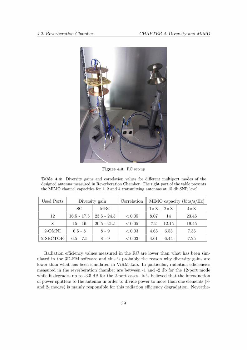
Measurements were performed in ’Bluetest AB’ premises on a RTS60 chamber whichcan support frequencies between 650 and 6000 MHz. Initially, a measurement of thereference antenna is taken with the antenna under test (AUT) inside the chamber (fig-ure 4.3). Then, measurements of the AUT’s ports are taken with the reference antennainside the chamber in order to have the chamber equally loaded as for the reference mea-surement. A 4-port VNA is used to collect the voltages at the antenna ports but sinceone of the VNA’s port is always connected to the source antenna, 3-ports where availablefor tracking receiving ports. Measurements were taken by using 12-, 8-, 2-OMNI and2-SECTOR modes between 1.7 and 2.2 GHz and diversity gain results, correlation valuesand MIMO capacities which are calculated according to [35] are presented in Table 4.4.
38
4.2. Reverberation Chamber CHAPTER 4. Diversity and MIMO
Figure 4.3: RC set-up
Table 4.4: Diversity gains and correlation values for different multiport modes of thedesigned antenna measured in Reverberation Chamber. The right part of the table presentsthe MIMO channel capacities for 1, 2 and 4 transmitting antennas at 15 db SNR level.
Used Ports Diversity gain Correlation MIMO capacity (bits/s/Hz)
SC MRC 1×X 2×X 4×X
12 16.5 - 17.5 23.5 - 24.5 < 0.05 8.07 14 23.45
8 15 - 16 20.5 - 21.5 < 0.05 7.2 12.15 19.45
2-OMNI 6.5 - 8 8 - 9 < 0.03 4.65 6.53 7.35
2-SECTOR 6.5 - 7.5 8 - 9 < 0.03 4.61 6.44 7.25
Radiation efficiency values measured in the RC are lower than what has been sim-ulated in the 3D-EM software and this is probably the reason why diversity gains arelower than what has been simulated in ViRM-Lab. In particular, radiation efficienciesmeasured in the reverberation chamber are between -1 and -2 db for the 12-port modewhile it degrades up to -3.5 dB for the 2-port cases. It is believed that the introductionof power splitters to the antenna in order to divide power to more than one elements (8-and 2- modes) is mainly responsible for this radiation efficiency degradation. Neverthe-
39

4.3. Channel Simulations CHAPTER 4. Diversity and MIMO
less, diversity gains achieved are still very high and can reach up to 24.5 dB when all 12ports are used. Spectral efficiency can reach up to 23.45 bits/s/Hz in an 4×12 MIMOsystem. It can also be seen that values of both diversity gain and capacity are quiteclose for OMNI and SECTOR modes; a fact that reinforces the notion that radiationpatterns play a minor role in a RIMP environment. Diversity gain and capacity plotstaken out of the RC measurements are presented in appendix C.
4.3 Channel Simulations
Channel simulations have been performed in Huawei’s channel emulator ’ACE’. In brief,the designed antenna is used as a base station (BS) multiport antenna within a networkcell where mobile users with specific location and velocity are spread. For each mobileuser a channel matrix H between the transmitter and the receiver is calculated basedon the Winner II channel model [36] and a capacity analysis is done and conclusionscan be drawn by observing the average values of capacity over a large number of mobileusers. Simulations have been done for an urban single cell network, that is, there isno interference between neighboring cells or between mobile users while mobile users’antennas are composed of one vertically and one horizontally polarized isotropic radiator.
In order to investigate the performance of the antenna, simulations have been per-formed in the same way as for diversity gain measurements; that is 12-, 8-, OMNI andSECTOR modes and initially it was investigated whether there is any difference in per-formance between 2-port antennas :
• having one electric and one magnetic dipole co-centered (dual polarized)
• having 2 electric dipoles in right angle
• having 2 electric dipoles placed λ distance apart
and as can be observed from figure C.9 the dual polarized dipole gives in total betterSNR than the other two cases and an increase in spectral efficiency of more than 1bps/Hz compared to the others.
The main goal of the simulations was to be investigated whether in an urban envi-ronment there is better performance when a directive beam towards a collection of usersis used instead of an omni-directional antenna. Therefore, capacity analysis has beendone for a collection of users confined in an certain angle ξ within the network cell asfigure 4.4 shows.
The final results are presented in figure 4.5 from which it can be seen (blue dashedline) that, as expected, the mean capacity stays on the same level regardless of thecoverage angle ξ since the location of a mobile user plays no role when the antenna isused in OMNI mode as it serves the whole cell equally with it’s omni-directional pattern.On the other hand, it can be seen (red dashed line) that the mean capacity is increasedwhen the antenna is used in SECTOR mode and users are confined in antenna’s beam.It can also be noted that the sector beam saturates around its 3dB-beamwidth angle (75- 85 degrees) where at that point provides 2 bps/Hz extra than the OMNI mode. When
40

4.3. Channel Simulations CHAPTER 4. Diversity and MIMO
Figure 4.4: Depiction of the coverage angle in a mobile cell.
the antenna is used in 12- or 8-port modes it always outperforms 2-port cases since itadapts with the optimal way to each user. Additionally, a capacity analysis for a quitenarrow beam has been also performed (black dashed line) and is presented in the sameplot. From the results of above analysis it can be concluded that although in a multipathenvironment it still make sense to direct the power of the antenna towards the locationthat users are located!
Figure 4.5: Capacity vs Confinement angle
41

5Conclusions and Future work
5.1 Conclusions
A multiport antenna, intended for base station use, has been designed and a prototypehas been implemented. The antenna is composed of 12 elements in an array configu-ration, can provide both horizontal and vertical polarizations and it is also shown howit can operate under different modes. Special interest presents the 2-port case, wherethe elements are configured in such a way that the antenna provides a two logical-portinterface. In particular, the vertically polarized elements are combined in order to pro-vide one vertically polarized radiation pattern and the horizontally polarized elementsare combined such that they give one horizontally polarized radiation pattern. In thisway, the two orthogonal polarizations can provide two very uncorrelated ports and thusbeing able to transmit two different streams of data at the same time; one through eachpolarization.
In addition, since the elements are positioned in an array configuration, they canprovide an additional feature; beamforming. Hence, by properly selecting the phaseexcitation of the elements in the antenna, the radiation pattern (of each polarization)can vary between omni-directional or sector beam which, additionally, can be stirredtowards four directions (±x, ±y). Diversity and channel simulations has shown thateven in a multipath environment, directing the energy towards the direction where theusers are located can increase the performance of the link. Hence, the designed antennacould be used in various environments regardless if it is preferable to have an omni-directional pattern or a sector beam.
The developed antenna presents a good impedance match (VWSR < 2) between1.7 and 2.2 GHz giving a bandwidth of around 25%. Coupling between neighboringelements is up to 12.5dB and coupling between cross polarized elements is as low as23dB. Simulated radiation patterns show an omni-directional rippling of maximum 3dBand when in SECTOR mode, a mainlobe/sidelobes difference which at minimum is at 8
42

5.2. Future work CHAPTER 5. Conclusions and Future work
and 10 dB for the horizontal and vertical polarization respectively.Measurements on the prototype regarding impedance match and coupling show great
similarity with the simulated values. The radiation patterns were also measured in ananechoic chamber and the results are very close to what has been simulated. Addition-ally, characterization of the antenna in terms of diversity and MIMO capacity has beenperformed in a reverberation chamber and result analysis showed that the antenna canachieve a diversity gain up to 24dB when all twelve elements are used and a spectral effi-ciency of more than 23 bps/Hz for a 4x12 MIMO system. Both channel simulations anddiversity measurements showed that the antenna performs better when all its elementsare individually used. For example, 12-ports perform better than 8-ports configurationwhich in turn performs better than 2-ports configuration. However, usage of more portsincrease the complexity of the system (more hardware, extra resources) so 2-port modecan be used when simplicity is of major importance. Overall, the designed antenna is aflexible implementation since it can adapt both in terms of complexity (different modes)and in terms of environment (omni/sector).
5.2 Future work
The performance of the antenna can be increased if the design of the horizontal com-ponents is further investigated. Although the existing loops give good omni-directional,horizontal polarized patterns with a quite wide impedance match, their diameter is wideand sets some restrictions regarding the array configuration. Smaller size would allowa closer spacing for the elements (< λ/2) hence the omni-directional rippling would bereduced and sidelobes level would be lower.
Feeding of the elements can also be reconsidered in order to provide an easier andmanufacture-friendly way to excite the elements. Instead of coaxial cables, planar trans-mission lines that follow the central metallic pole and spread on the three planes canbe used as a feeding network. In this way, it would also be easier to use more than oneantenna in a stacked configuration in order to increase directivity and/or total numberof ports.
43

Bibliography
[1] C. A. Balanis, Antenna Theory : Analysis and Design, John Wiley & Sons, Inc.,2005.
[2] P. S. Kildal, Foundations of Antennas : A unified approach for Line-Of-Sight andMultipath, 2013.
[3] R. Yadava, Antenna and Wave Propagation, Phi Learning Private Limited, 2011.
[4] A. Ludwig, Mutual coupling, gain and directivity of an array of two identical an-tennas, Antennas and Propagation, IEEE Transactions on 24 (6) (1976) 837–841.
[5] A. Goldsmith, Wireless Communications, Cambridge University Press, 2005.
[6] P. S. Kildal, K. Rosengren, Correlation and capacity of mimo systems and mu-tual coupling, radiation efficiency, and diversity gain of their antennas: simulationsand measurements in a reverberation chamber, Communications Magazine, IEEE42 (12) (2004) 104–112.
[7] T. Brown, E. De Carvalho, P. Kyritsi, Practical Guide to the MIMO Radio Channelwith MATLAB Examples, John Wiley & Sons, 2012.
[8] X. Chen, B. Einarsson, P.-S. Kildal, Improved mimo throughput with inverse powerallocation - study using usrp measurement in reverberation chamber, Antennas andWireless Propagation Letters, IEEE 13 (2014) 1494–1496.
[9] M. A. Solano, A. Vegas, A. Gomez, On the use of auxiliary vector potentials as acommon tool for studying electromagnetic problems at undergraduate level, Inter-national Journal of Electrical Engineering Education 40 (2) (2003) 123.
[10] S.-W. Lee, J.-H. Lee, Electrically small mng zor antenna with multilayered conduc-tor, IEEE Antennas and Wireless Propagation Letters 1 (2010) 724–727.
[11] J.-H. Park, Y.-H. Ryu, J.-H. Lee, Mu-zero resonance antenna, IEEE Transactionson Antennas and Propagation 54 (6) (2010) 1865–1875.
44

BIBLIOGRAPHY BIBLIOGRAPHY
[12] K. Wei, Z. Zhang, Z. Feng, M. F. Iskander, A mng-tl loop antenna array withhorizontally polarized omnidirectional patterns, IEEE Transactions on Antennasand Propagation 60 (6) (2012) 2702–2710.
[13] K. Wei, Z. Zhang, Z. Feng, Design of a wideband horizontally polarized omnidirec-tional printed loop antenna, IEEE Antennas and Wireless Propagation Letters 11(2012) 49–52.
[14] A. Alford, A. G. Kandoian, Ultrahigh-frequency loop antennas, Transactions of theAmerican Institute of Electrical Engineers 59 (12) (1940) 843–848.
[15] H. Chuang, T. Horng, J. Pan, C. Wang, Omni-directional horizontally polarizedalford loop strip antenna, uS Patent 5,767,809 (Jun. 16 1998).URL http://www.google.co.uk/patents/US5767809
[16] C.-C. Lin, H. R. Chuang, A 2.4ghz planar printed antenna with omni-directionalhorizontally polarized pattern for wlan applications, in: Microwave Conference,2003. 33rd European, 2003, pp. 1275–1278.
[17] X. Quan, R. Li, J. Wang, Y. Cui, Development of a broadband horizontally po-larized omnidirectional planar antenna and its array for base stations, Progress InElectromagnetics Research 128 (2012) 441–456.
[18] C.-H. Ahn, S.-W. Oh, K. Chang, A dual-frequency omnidirectional antenna forpolarization diversity of mimo and wireless communication applications, Antennasand Wireless Propagation Letters, IEEE 8 (2009) 966–969.
[19] C. Jiang, X. W. Dai, Y.-C. Jiao, A novel compact horizontally polarized omni-directional antenna, in: Signals Systems and Electronics (ISSSE), 2010 InternationalSymposium on, Vol. 1, 2010, pp. 1–3.
[20] Y. Yu, F. Jolani, Z. Chen, A wideband omnidirectional horizontally polarized an-tenna for 4g lte applications, Antennas and Wireless Propagation Letters, IEEE 12(2013) 686–689.
[21] J. I. Kim, B. M. Lee, Y. J. Yoon, Wideband printed dipole antenna for multiplewireless services, 2001, pp. 153–156.
[22] G. Chen, J. Sun, A printed dipole antenna with microstrip tapered balun, Microwaveand Optical Technology Letters 40 (4) (2004) 344–346.
[23] Y. Wang, L. Yang, S. Gong, X. Feng, J. Wang, Omnidirectional antenna with dipolearray, IEEE, 2012, pp. 347–348.
[24] B. G. Duffley, G. A. Morin, M. Mikavica, Y. M. M. Antar, A wide-band printeddouble-sided dipole array, IEEE Transactions on Antennas and Propagation 52 (2)(2004) 628–631.
45

BIBLIOGRAPHY
[25] K. P. Ray, Design aspects of printed monopole antennas for ultra-wide band appli-cations, International Journal of Antennas and Propagation 2008 (2008) 1–8.
[26] A. V. S. Lages, V. Dmitriev, M. N. Kawakatsu, D. C. Nascimento, D. B. Ferreira,E. S. Costa, Ultr-wideband planar monopole antennas with improved characteris-tics, Microwave and Optical Technology Letters 55 (9) (2013) 2149–2154.
[27] R. A. Sadeghzadeh, Y. Zehforoosh, N. Mirmotahhary, Ultra-wideband monopoleantenna with modified triangular patch, Microwave and Optical Technology Letters53 (8) (2011) 1752–1756.
[28] M. Ammann, Square planar monopole antenna, in: Antennas and Propagation,1999. IEE National Conference on., 1999, pp. 37–40.
[29] Z. N. Chen, Broadband planar monopole antenna, IEE Proceedings - Microwaves,Antennas and Propagation 147 (6) (2000) 526.
[30] P. Kildal, C. Orlenius, J. Carlsson, Ota testing in multipath of antennas and wirelessdevices with mimo and ofdm, Vol. 100, IEEE, 2012, pp. 2145–2157.
[31] P. Kildal, K. Rosengren, J. Byun, J. Lee, Definition of effective diversity gain andhow to measure it in a reverberation chamber, Microwave and Optical TechnologyLetters 34 (1) (2002) 56–59.
[32] P.-S. Kildal, U. Carlberg, J. Carlsson, Definition of antenna diversity gain in user-distributed 3d-random line-of-sight, Journal of electromagnetic engineering and sci-ence 13 (2) (2013) 86–92.
[33] U. Carlberg, J. Carlsson, A. Hussain, P. S. Kildal, Ray based multipath simulationtool for studying convergence and estimating ergodic capacity and diversity gain forantennas with given far-field functions, in: ICECom, 2010 Conference Proceedings,2010, pp. 1–4.
[34] P.-S. Kildal, X. Chen, C. Orlenius, M. Franzen, C. S. L. Patane, Characterizationof reverberation chambers for ota measurements of wireless devices: Physical for-mulations of channel matrix and new uncertainty formula, IEEE Transactions onAntennas and Propagation 60 (8) (2012) 3875–3891.
[35] X. Chen, P.-S. Kildal, J. Carlsson, J. Yang, Mrc diversity and mimo capacity eval-uations of multi-port antennas using reverberation chamber and anechoic chamber,IEEE Transactions on Antennas and Propagation 61 (2) (2013) 917–926.
[36] WINNER Phase II Model, http://www.ist-winner.org/phase_2_model.html
(2007).
46

AMathematical expressions for
radiating fields
General expressions for radiating fields
If the electric surface current and the magnetic surface current, J andM respectively,are known then the general radiation expressions are given by [2]:
E(r) = EJ(r) +EM (r) (A.1)
H(r) = HJ(r) +HM (r) (A.2)
where
EJ = Ck
∫∫
S′
[
ηJCN1 − (ηJ · R)R CN2
] 1
Re−jkR dS′ (A.3)
HJ = −1
ηCk
∫∫
S′
(
ηJ · R)
CN1
Re−jkR dS′ (A.4)
EM = Ck
∫∫
S′
(
M · R)
CN1
Re−jkR dS′ (A.5)
HM =1
ηCk
∫∫
S′
[
MCN1 − (M · R)R CN2
] 1
Re−jkR dS′ (A.6)
with Ck = −jk/(4π), CN = 1 + 1jkR , CN1 = 1 + 1
jkR − 1(kR)2
, CN2 = 1 + 3jkR − 3
(kR)2
and where S′ is the surface of the radiating element, r′ is the current vector, r is theobservation point and R = r− r′, R = |r − r′|, R = R/R.
47

CHAPTER A. Mathematical expressions for radiating fields
When in far-field, the Fraunhofer approximation can be applied, thus:
E(r) =1
re−jkr IJ − (IJ · r) r+ IM × r (A.7)
H(r) =1
ηr×E =
1
ηre−jkr r× IJ + [IM − (IM · r)r] (A.8)
where
IJ = Ck
∫∫
S′
ηJ(r′)ejk(r′·r)dS′ (A.9)
IM = Ck
∫∫
S′
M(r′)ejk(r′·r)dS′ (A.10)
are the electric and magnetic radiation integrals.
Integral formula used in dipole’s radiating field:
∫
eαx sin(βx+ γ)dx = eαx1
α2 + β2[α sin(βx+ γ)− β cos(βx+ γ)] (A.11)
3-Dimensional Characteristics
For a vector r with magnitude r = |r|, conversion from spherical to rectangularcoordinate system can be obtained through the following equations :
x = r sin θ cosφ x
y = r sin θ sinφ y
z = r cos θ z (A.12)
The angle γ between one axis and an observation point can be obtained by the dotproduct of a unit vector along this axis and a unit vector towards the observation point.If the elements of a linear array are along the z-axis then they have a symmetry in respectto this axis and are independent of the φ angle because :
cos γ = az · ar = az · (ax sin θ cosφ+ ay sin θ sinφ+ ˆaz cos θ) = cos θ → γ = θ (A.13)
On the other hand, if elements are positioned along x or y axis then angle γ is dependentof both θ and φ angles as can be seen from the following equations :
cos γ = az · ar = az · (ax sin θ cosφ+ ay sin θ sinφ+ ˆaz cos θ) = sin θ cosφ→→ γ = cos−1(sin θ cosφ) (A.14)
48

CHAPTER A. Mathematical expressions for radiating fields
and
cos γ = az · ar = az · (ax sin θ cosφ+ ay sin θ sinφ+ ˆaz cos θ) = sin θ sinφ→→ γ = cos−1(sin θ sinφ) (A.15)
49

BAntenna Structure figures
Figure B.1: View 1 of the HPol Array. Middle plane contains the 4 horizontal polarizedelements and the other two are the ground planes
50

CHAPTER B. Antenna Structure figures
Figure B.2: View 2 of the HPol Array. Radius of the ground plane and the hollow centralmetal tube.
Figure B.3: View 3 of the HPol Array. Dimensions of the middle plane.
51

CHAPTER B. Antenna Structure figures
Figure B.4: Dimensions of the ground plane and positioning of the monopoles.
52

CHAPTER B. Antenna Structure figures
Figure B.5: Maximal distance (y) between two magnetic dipoles. x = 2 ∗ (L1 + L2) and
y =√2 ∗ x2
53

CHAPTER B. Antenna Structure figures
(a)
(b)
Figure B.6: Feeding of the magnetic dipole. Inner conductor of the coaxial cable is solderedto the top metal (up) and outer conductor to the bottom metal (down).
54

CHAPTER B. Antenna Structure figures
(a)
(b)
Figure B.7: Feeding of the monopole patches. The Inner conductor of the coaxial cableis soldered to the feeding patch (up) and the outer conductor to the outer surface of theground plane (down).
55

CHAPTER B. Antenna Structure figures
Figure B.8: Top view of the prototype antenna
56

CHAPTER B. Antenna Structure figures
Figure B.9: Bottom view of the prototype antenna
57

CReverberation Chamber and
channel simulation
58

CHAPTER C. Reverberation Chamber and channel simulation
Figure C.1: CDF plots and effective gain of the 12-port antenna
Figure C.2: Spectral efficiency plot of the 4 × 12 MIMO channel
59

CHAPTER C. Reverberation Chamber and channel simulation
Figure C.3: CDF plots and effective gain of the 8-port antenna
Figure C.4: Spectral efficiency plot of the 4 × 8 MIMO channel
60

CHAPTER C. Reverberation Chamber and channel simulation
Figure C.5: CDF plots and effective gain of the 2-port OMNI-mode antenna
Figure C.6: Spectral efficiency plot of the 4 × 2 MIMO channel
61

CHAPTER C. Reverberation Chamber and channel simulation
Figure C.7: CDF plots and effective gain of the 2-port SECTOR-mode antenna
Figure C.8: Spectral efficiency plot of the 4 × 2 MIMO channel
62

CHAPTER C. Reverberation Chamber and channel simulation
(a)
(b)
(c)
Figure C.9: Plots for SNR of eigenchannel 1, eigenchannel 2 and spectral efficiency re-spectively. Red lines indicate the dual polarized antenna, blue lines indicate two orthogonalelectric dipoles and the purple one indicates two electrical dipoles placed one λ apart.
63

DReturn Loss and coupling
Figure D.1: Bandwidth of the original antenna as proposed by [20] but without parasiticstrips.
64

CHAPTER D. Return Loss and coupling
Figure D.2: Parametric study on horizontally polarized omni-directional antenna’s angleA. Bandwidth increases as angle A increases.
Figure D.3: Parametric study on horizontally polarized omni-directional antenna’s size.The resonance frequency moves lower in the spectrum as the size of the antenna increases.
65

CHAPTER D. Return Loss and coupling
Figure D.4: Parametric study on horizontally polarized omni-directional antenna’s size.The resonance frequency moves lower in the spectrum as the width of the dipole arm in-creases.
66

CHAPTER D. Return Loss and coupling
(a) Return Loss of Monopoles
(b) Return Loss of magnetic dipoles
Figure D.5: Return loss of the dual polarized antenna.
67

CHAPTER D. Return Loss and coupling
(a) Coupling between monopole elements
(b) Coupling between magnetic dipole elements
(c) Coupling between orthogonal polarized elements
Figure D.6: Coupling of the dual polarized antenna.
68

CHAPTER D. Return Loss and coupling
Figure D.7: Return loss of the magnetic dipoles as measured on a 2-port VNA. The blackdashed line indicates the simulated return loss.
Figure D.8: Return loss of the monopole patches as measured on a 2-port VNA. Theblack dashed line indicates the initially simulated return loss while the dotted line shows thesimulated return loss for the expanded substrate case.
69

CHAPTER D. Return Loss and coupling
Figure D.9: Coupling levels between magnetic dipoles. Purple line shows coupling valuesfor adjacent dipoles while yellow line shows coupling between opposite dipoles. Dashed linesindicate the simulated values.
Figure D.10: Coupling levels between monopole patches. Dashed line represent simulatedvalues for adjacent and opposite elements.
70

CHAPTER D. Return Loss and coupling
Figure D.11: Coupling levels between vertical and horizontal polarized elements.
71

ERadiation Patterns
72

CHAPTER E. Radiation Patterns
(a) Phi-cut (b) Theta-cut (c) 3D pattern
(d) Phi-cut (e) Theta-cut (f) 3D pattern
(g) Theta-cut (h) Theta-cut (i) 3D pattern
Figure E.1: Horizontal polarized omni-directional antenna radiation pattern @ 1.7, 2 and 2.2 GHz.Both co-polar and cross-polar components are depicted.
73

CHAPTER E. Radiation Patterns
(a) λ/4 distance (b) λ/2 distance (c) λ/1.5 distance
Figure E.2: Azimuth (up) and elevation (down) cuts when in OMNI mode for threedifferent element distances.
(a) λ/4 distance (b) λ/2 distance (c) λ/1.5 distance
Figure E.3: Azimuth (up) and elevation (down) cuts when in SECTOR mode for threedifferent element distances.
74

CHAPTER E. Radiation Patterns
(a) Phi-cut (b) Theta-cut (c) 3D pattern
(d) Phi-cut (e) Theta-cut (f) 3D pattern
(g) Phi-cut (h) Theta-cut (i) 3D pattern
Figure E.4: Horizontal polarized Array radiation pattern in OMNI mode @ 1.7, 2 and 2.2 GHz.
75

CHAPTER E. Radiation Patterns
(a) Phi Cut (b) 3D pattern
(c) Phi Cut (d) 3D pattern
(e) Phi Cut (f) 3D pattern
Figure E.5: Horizontal polarized Array radiation pattern in SECTOR mode @ 1.7, 2 and2.2 GHz
76
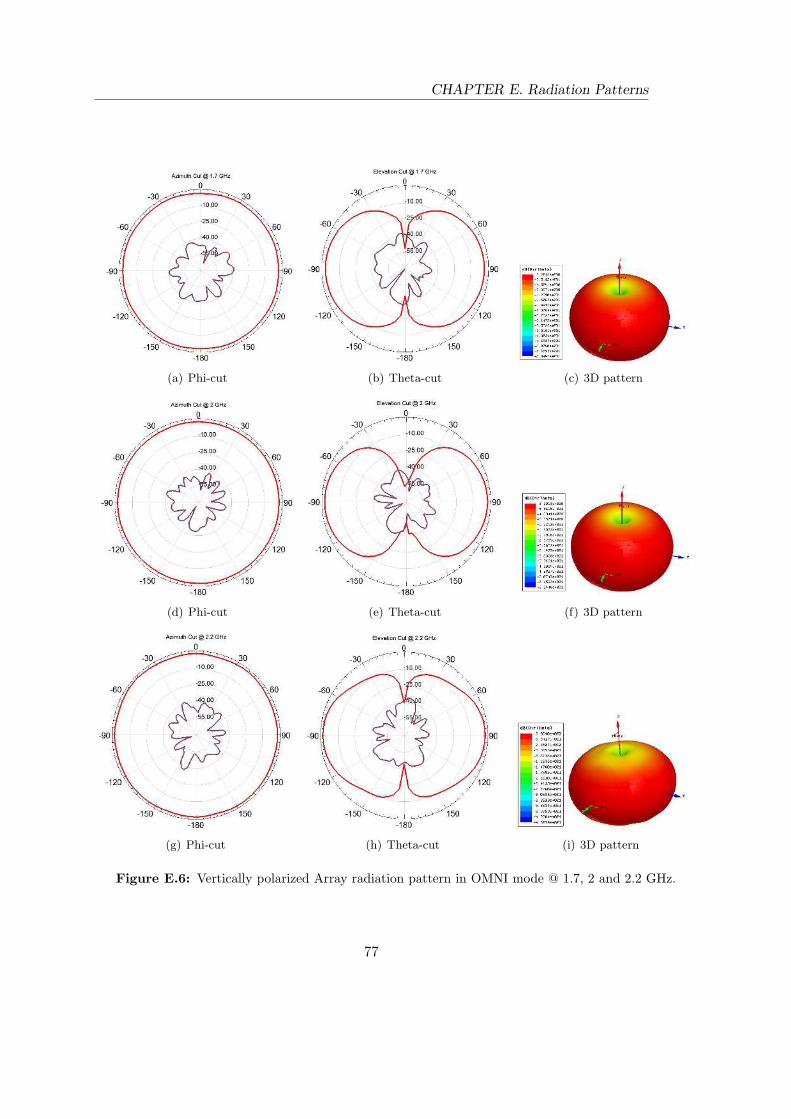
CHAPTER E. Radiation Patterns
(a) Phi-cut (b) Theta-cut (c) 3D pattern
(d) Phi-cut (e) Theta-cut (f) 3D pattern
(g) Phi-cut (h) Theta-cut (i) 3D pattern
Figure E.6: Vertically polarized Array radiation pattern in OMNI mode @ 1.7, 2 and 2.2 GHz.
77

CHAPTER E. Radiation Patterns
(a) Phi Cut (b) 3D pattern
(c) Phi Cut (d) 3D pattern
(e) Phi Cut (f) 3D pattern
Figure E.7: Vertical polarized Array radiation patterns in SECTOR mode @ 1.7, 2 and2.2 GHz
78

CHAPTER E. Radiation Patterns
(a) Phi cut (b) Phi cut (c) Phi cut
(d) Thetta cut (e) Thetta cut (f) Thetta cut
(g) 3D pattern (Vertical Polariza-tion)
(h) 3D pattern (Vertical Polariza-tion)
(i) 3D pattern (Vertical Polarization)
(j) 3D pattern (Horizontal Polariza-tion)
(k) 3D pattern (Horizontal Polariza-tion)
(l) 3D pattern (Horizontal Polariza-tion)
Figure E.8: Dual Polarized antenna - OMNI mode @ 1.7, 2 and 2.2 GHz. Red line : Verticalpolarized component, Blue line : Horizontal Polarized component
79

CHAPTER E. Radiation Patterns
Table E.1: Elevation and azimuth 3dB (full angle) beam-width simulated values for bothpolarizations and every mode (OMNI, SECTOR and optimized SECTOR).
Freq Elevation 3dB BW Azimuth 3dB BW
Vertical Horizontal Vertical Horizontal
OMNI 2.2G 50o 59o - -
2G 56.5o 68o - -
1.7G 66o 110o - -
SECTOR 2.2G 51o 64o 74o 74o
2G 57.5o 109o 80o 90o
1.7G 65o 80o 89o 70o
Opt.SEC 2.2G 52o 69o 73o 76o
2G 66o 115o 75.5o 92o
1.7G 75o 86o 74o 82o
80

CHAPTER E. Radiation Patterns
(a) Phi cut
(b) Phi cut
(c) Phi cut
Figure E.9: Dual Polarized antenna - SECTOR mode @ 1.7, 2 and 2.2 GHz. Red line :Vertical polarized component, Blue line : Horizontal Polarized component
81

CHAPTER E. Radiation Patterns
(a)Phicu
t@
2GHz,
HorizontalPolarization
(b)Thetacu
t@
2GHz,
HorizontalPolarization
(c)Phicu
t@
2.2GHz,
HorizontalPolarization
(d)Thetacu
t@
2.2GHz,
HorizontalPolarization
FigureE.10:Measuredradiation
patternsof
theHorizon
talcompon
ents
at2an
d2.2
GHzforOMNImode.
Bluelines
indicate
Horizon
talPolarization(co-polar)an
dredlines
indicateVerticalPolarization(cross-polar).Dashed
lines
indicate
thecorresponding
simulatedpatterns.
82

CHAPTER E. Radiation Patterns
(a)Phicu
t@
2GHz,
VerticalPolarization
(b)Thetacu
t@
2GHz,
VerticalPolarization
(c)Phicu
t@
2.2GHz,
VerticalPolarization
(d)Thetacu
t@
2.2GHz,
VerticalPolarization
Figure
E.11:
Measuredradiation
patternsof
theVerticalcompon
ents
at2an
d2.2
GHzforOMNImode.
Bluelines
indicate
Horizon
talPolarization(cross-polar)an
dredlines
indicateVerticalPolarization(co-polar).Dashed
lines
indicate
thecorresponding
simulatedpatterns.
83

CHAPTER E. Radiation Patterns
(a)HorizontalPolarizedSECTOR
beam
@2GHz
(b)VerticalPolarizedSECTOR
beam
@2GHz
(c)HorizontalPolarizedSECTOR
beam
@2.2GHz
(d)VerticalPolarizedSECTOR
beam
@2.2GHz
FigureE.12:Measuredradiation
patternsof
theHorizon
talan
dVerticalcompon
ents
at2and2.2
GHzforSECTOR
mode.
Blue
lines
indicateHorizon
talPolarizationan
dredlines
indicateVerticalPolarization.Dashed
lines
indicate
thecorrespondingsimulated
patterns.
84

FHFSS vs CST studio suite
The final antenna structure was designed and simulated in two different 3D electromag-netic simulation softwares, Ansys HFSS 2014.0.7 and CST Studio Suite 2013 v.2013.06 .HFSS solver was used as a frequency domain solver while CST as a time domain solver.
In HFSS, EM analysis in three different frequencies (2.2GHz, 2GHz and 1.7GHz)was set up together with a frequency sweep of 21 samples between 1.5GHz and 2.5GHzfor calculation of S-parameters. At 2.2GHz, mesh adaptation took about an hour tocomplete, producing 377114 tetrahedrons and together with the frequency sweep required3h and 25min to finish. At 2 GHz adaptation took about 2h and 20min producing 549892tetrahedrons and at 1.7GHz mesh adaptation needed 5h and 43 min, producing 950432tetrahedrons. In total, the whole simulation required 11h and 28min and at maximum34.4GB of RAM to complete.
In CST Studio suite, the hexahedral cell mesh was chosen with manual (uniform)definition of mesh. Again, field monitors and radiation patterns were setup at frequencies2.2GHz, 2GHz and 1.7GHz and a frequency range between 1.5 and 2.5 Gigahertz . Thehexahedral mesh was formed by 15.291.360 cells and the total required simulation timewas 26h and 59min while the maximum required memory was at 5.6GB. The requiredsimulation time is way longer than HFSS but it is believed that with a more carefulinitial mesh formation, less cells may produced which will lead to shorter simulationtime.
In general, the two softwares produced identical results (S-parameters, Radiationpatterns, radiation efficiencies ...). Indicatively, some S-parameters plots are presentedbelow to show the similarity of the results.
85

CHAPTER F. HFSS vs CST studio suite
(a)
(b)
FigureF.1:HFSSvsCST
return
loss
plots.Loop
s(U
p)an
dMon
opoles
(Dow
n)are
presented.Red
solidlineindicatesHFSS
resultsan
dblack
dashed
lineindicates
CST
result.
(a)
(b)
FigureF.2:HFSSvsCST
couplingplots.Loop
s(U
p)an
dMon
opoles
(Dow
n)arepresented.Red
solidlineindicatesHFSSresults
andblack
dashed
lineindicates
CST
result.
86