miguel a. segoviano and charles goodhart - imf · banking stability measures prepared by miguel a....

WP/09/4

Banking Stability Measures

Miguel A. Segoviano and Charles Goodhart

© 2009 International Monetary Fund WP/09/4 IMF Working Paper Monetary and Capital Markets Department

Banking Stability Measures

Prepared by Miguel A. Segoviano and Charles Goodhart1

Authorized for distribution by Mark Swinburne

January 2009

Abstract

This Working Paper should not be reported as representing the views of the IMF. The views expressed in this Working Paper are those of the author(s) and do not necessarily represent those of the IMF or IMF policy. Working Papers describe research in progress by the author(s) and are published to elicit comments and to further debate.

This paper defines a set of banking stability measures which take account of distress dependence among the banks in a system, thereby providing a set of tools to analyze stability from complementary perspectives by allowing the measurement of (i) common distress of the banks in a system, (ii) distress between specific banks, and (iii) distress in the system associated with a specific bank. Our approach defines the banking system as a portfolio of banks and infers the system’s multivariate density (BSMD) from which the proposed measures are estimated. The BSMD embeds the banks’ default inter-dependence structure that captures linear and non-linear distress dependencies among the banks in the system, and its changes at different times of the economic cycle. The BSMD is recovered using the CIMDO-approach, a new approach that in the presence of restricted data, improves density specification without explicitly imposing parametric forms that, under restricted data sets, are difficult to model. Thus, the proposed measures can be constructed from a very limited set of publicly available data and can be provided for a wide range of both developing and developed countries. JEL Classification Numbers: C02, C19, C52, C61, E32, G21 Keywords: Financial stability; portfolio risk; copula functions; entropy distribution. Authors’ E-Mail Addresses: [email protected]; [email protected] 1 The authors would especially like to thank S. Neftci, R. Rigobon (MIT), H. Shin (Princeton), D. Tsomocos (Oxford), O. Castren, M. Sydow, J. Fell (ECB), T. Bayoumi, K. Habermeier, A. Tieman (IMF), for helpful comments and discussions, and inputs from participants in the seminar series/conferences at the MCM/IMF, ECB, Morgan Stanley, BoE, Banca d’Italia, Columbia University, Deutsche BuBa/Banque de France and Riksbank.

2

Contents Page

I. Introduction ............................................................................................................................4

II. Distress Dependence among Banks and Stability of the Banking System ...........................7

III. Banking System Multivariate Density .................................................................................9 A. The CIMDO Approach: Modeling the Banking System Multivariate Density ........9 B. The CIMDO-copula: Distress Dependence among Banks in the System...............11

IV. Banking Stability Measures...............................................................................................16 A. Common Distress in the Banks of the System........................................................17 B. Distress Between Specific Banks............................................................................18 C. Distress in the System Associated with a Specific Bank ........................................18

V. Banking Stability Measures: Empirical Results..................................................................19 A. Estimation of Probabilities of Distress of Individual Banks...................................20 B. Examination of Relative Changes of Stability over Time.......................................21 C. Analysis of Cross-Region Effects Between Different Banking Groups .................27 D. Analysis of Foreign Banks’ Risks to Sovereigns with Banking Systems with

Cross-Border Institutions .......................................................................................28

VI. Conclusions........................................................................................................................36 References................................................................................................................................49 Tables 1. Distress Dependence Matrix ................................................................................................18 2. Distress Dependence Matrix: American and European Banks ............................................29 3. Distress Dependence Matrix: Latin America. Sovereigns and Banks .................................33 4. Distress Dependence Matrix: Eastern Europe. Sovereigns and Banks................................34 5. Distress Dependence Matrix: Asia. Sovereigns and Banks .................................................35 Figures 1. The Probability of Distress ....................................................................................................8 2. The Banking System’s Multivariate Density.........................................................................9 3. Probability That At Least One Bank Becomes Distressed ..................................................19 4. Joint Probability of Distress.................................................................................................23 5. Banking Stability Index .......................................................................................................24 6. Daily Percentage Increase: Joint and Average Probability of Distress................................25 7. PAO: Lehman ......................................................................................................................26 8. Foreign-Bank and Sovereign Risks .....................................................................................32 Box 1. Drawbacks to the Characterization of Distress Dependence of Financial Returns with Correlations..............................................................................................................................14

3

Appendixes I. Copula Functions..................................................................................................................37 II. CIMDO-copula....................................................................................................................39 III. CIMDO-density and CIMDO-copula Evaluation Framework ..........................................40 IV. Estimation of Probabilities of Distress of Individual Banks .............................................47

4

I. INTRODUCTION

Economics is a quantitative science. Macroeconomics depends on data for national income, expenditure and output variables. Macro-monetary policy requires measures of inflation. Microeconomics is based on data for prices and quantities of inputs and outputs. Even when the variables of concern are difficult to measure, such as the output gap, expectations, and ‘happiness’, we use various techniques, e.g. survey data, to provide quantitative proxy variables—often according these data more weight than is consistent with their inherent measurement errors. Without such quantification, comparisons over time, and on a cross-section basis, cannot be made; nor would it be easy to provide a quantified analysis of the determinants of such variables. However, there is currently no such widely accepted measure, quantification, or time series for measuring either financial or banking stability. What is most often used instead is an on/off (1/0) assessment of whether a ‘crisis’ has occurred.2 This has then been used to review whether there have been common factors preceding, possibly even causing, such crises, and to assess what official responses have best mitigated such crises, see Bank Restructuring and Resolution, ed. Hoelscher, (2006). While much useful research has been done employing a crisis on/off dichotomy, it has several inherent deficiencies. In particular, the lack of a continuous scale makes it impossible to measure with sufficient accuracy either (i) the relative riskiness of the system in non-crisis mode, or (ii) the intensity of a crisis, once it has started. If the former could be measured, it may be easier to take early remedial action as the danger of a systemic crisis increases, while measurement of the latter would facilitate decision making on the most appropriate measures to address the crisis. In our view, a precondition for improving the analysis and management of financial (banking) stability is to be able to construct a metric for it. The purpose of this paper is therefore to present a method for estimating a set of stability measures of the banking system (BSMs). There is no unique, best way to estimate BSMs, any more than there is a unique best way to measure such concepts as ‘output’ or ‘inflation’, but we hope to demonstrate that our approach is reasonable. Moreover, there are very few alternative available measures which might be used. Briefly, and as described in far more detail below, we conceptualize the banking system as a portfolio of banks comprising the core, systemically important banks in any country. Thus, we infer the banking system’s portfolio multivariate density (BSMD) from which we construct a set of BSMs. These measures embed the banks’distress inter-dependence structure, which captures not only linear (correlation) but also non-linear distress dependencies among the banks in the system. Moreover, the structure of linear and non-linear distress dependencies changes as banks’ probabilities of distress (PoDs) change; hence,

2 For a review of the literature on financial crises, see Bordo (2001).

5

the proposed stability measures incorporate changes in distress dependence that are consistent with the economic cycle. This is a key advantage over traditional risk models that most of the time incorporate only linear dependence (correlation structure), and assume it constant throughout the economic cycle. 3 Consequently, the proposed BSMs represent a set of tools to analyze (define) stability from four different, yet, complementary perspectives, by allowing the quantification of (a) “common” distress in the banks of the system, (b) distress between specific banks, and (c) distress in the system associated with a specific bank. In this paper we estimate the proposed BSMs using publicly available information from 2005 up to the beginning of October 2008. These estimations are to illustrate the methodology rather than to make an assessment of the conjunctural financial stability of any particular system. We examine relative changes in stability over time and among different banks’ business lines in the US banking system. We also analyze cross-region effects between American and European banking groups. Lastly, we show how our technique can be extended to incorporate the effect of foreign banks on sovereigns with banking systems with cross-border institutions. For this purpose, we estimate the BSMs for major foreign banks and sovereigns in Latin America, eastern Europe and Asia. This implementation flexibility is of relevance for banking stability surveillance, since cross-border financial linkages are growing and becoming significant; as has been highlighted by the financial market turmoil of recent months. Thus, surveillance of banking stability cannot stop at national borders. We show how these BSMs can be constructed from a very limited set of data, e.g., empirical measurements of distress of individual banks. Such measurements can be estimated using alternative approaches, depending on data availability; thus, the data set that is necessary to estimate the BSMs is available in most countries. Consequently, such measures can be provided for a wide group of developing, as well as developed, countries. Being able to establish such a set of measures with a minimum of basic components, makes it feasible to undertake a wider range of comparative analysis, both time series and cross-section. It is important to note that when measurements of distress of non-banking financial institutions (NBFIs) i.e., insurance companies, hedge funds etc. are available, our methodology can be easily extended to incorporate the effects of such institutions in the measurement of stability, hence allowing us to estimate a set of stability measures for the financial system. This could be of relevance for countries where NBFIs have systemic importance in the financial sector.

3 In contrast to correlation, which only captures linear dependence, copula functions characterize the whole dependence structure; i.e., linear and non-linear dependence, embedded in multivariate densities (Nelsen, 1999). Thus, in order to characterize banks’ distress dependence we employ a novel non-parametric copula approach; i.e., the CIMDO-copula (Segoviano, 2009), described below. In comparison to traditional methodologies to model parametric copula functions, the CIMDO-copula avoids the difficulties of explicitly choosing the parametric form of the copula function to be used and calibrating its parameters, since CIMDO-copula functions are inferred directly (implicitely) from the joint movements of the individual banks’ PoDs.

6

Economically, our approach is based on the micro-founded, general equilibrium theoretical framework of Goodhart, Sunirand and Tsomocos (2006), which indicates that financial instability can arise either through systemic shocks, contagion after idiosyncratic shocks or a combination of both. In this respect, our proposed banking system stability measures represent a clear improvement over purely statistical or mathematical models that are economically a-theoretical and therefore difficult to interpret. Over the past decade, we have completed a research agenda that has allowed us to gain important insights into the analysis of financial stability. For example, in Segoviano (1998), Segoviano and Lowe (2002), and Goodhart and Segoviano (2004), we present simple approaches that vary in the degree of sophistication to quantify portfolio credit risk (all of these approaches were based on parametric models, and accounted only for correlations that were fixed through the cycle) and analyze the procyclicality of banking regulation and its implications for financial stability. In Segoviano and Padilla (2006), we present a framework for macroeconomic stress testing combined with a model for portfolio credit risk evaluation, which accounts for linear and non-linear dependencies among the assets in banks’ portfolios and their changes across the economic cycle; however, in all these cases, we focus on individual banks’ portfolios or in the overall aggregate banking system. In Goodhart, Hofmann and Segoviano (2004, 2006), and Aspachs et al. (2006) we focus on systemic risk, making use of average measurements of distress of the system, which do not incorporate banks’ distress dependencies, nor their changes across the economic cycle. Thus, we hope that the proposed BSMs will allow us to complement our previous research and gain further insights into our understanding of financial stability. We are therefore extending our research as follows in order to achieve specific aims.

i. We examine relative changes in the BSMs over time and between countries, in order to identify the occasion, and determinants, of changes in the riskiness of the banking system;

ii. We try to predict future movements of the BSMs for use as an early-warning mechanism;

iii. We explore the significant macroeconomic and financial factors and shocks influencing the BSMs, in order to identify macro-financial linkages; and

iv. We explore the factors that can limit and reverse tendencies towards instability, so as to discover what instruments may be available (and under what conditions) to control such instability.

In Section II, we explain the importance of incorporating banks’ distress dependence in the estimation of the stability of the banking system and describe the modeling steps followed in our framework. In Section III, we present the consistent information multivariate density (CIMDO) methodology to infer the banking system’s multivariate density (BSMD) from which the proposed BSMs are estimated. These are defined in Section IV. In Section V, we

7

present empirical estimates of the proposed BSMs as described above. Finally, conclusions are presented in Section VI.

II. DISTRESS DEPENDENCE AMONG BANKS AND STABILITY OF THE BANKING SYSTEM

The proper estimation of distress dependence amongst the banks in a system is of key importance for the surveillance of stability of the banking system. Financial supervisors recognize the importance of assessing not only the risk of distress i.e., large losses and possible default of a specific bank, but also the impact that such an event would have on other banks in the system. Clearly, the event of simultaneous large losses in various banks would affect a banking system’s stability, and thus represents a major concern for supervisors. Bank’s distress dependence is based on the fact that banks are usually linked—either directly, through the inter-bank deposit market and participations in syndicated loans, or indirectly, through lending to common sectors and proprietary trades. Banks’ distress dependence varies across the economic cycle, and tends to rise in times of distress since the fortunes of banks decline concurrently through either contagion after idiosyncratic shocks, affecting inter-bank deposit markets and participations in syndicated loans—direct links—or through negative systemic shocks, affecting lending to common sectors and proprietary trades—indirect links. Therefore, in such periods, the banking system’s joint probability of distress (JPoD); i.e., the probability that all the banks in the system experience large losses simultaneously, which embeds banks’ distress dependence, may experience larger and nonlinear increases than those experienced by the probabilities of distress (PoDs) of individual banks. Consequently, it becomes essential for the proper estimation of the banking system’s stability to incorporate banks’ distress dependence and its changes across the economic cycle. Quantitative estimation of distress dependence, however, is a difficult task. Information restrictions and difficulties in modeling distress dependence arise due to the fact that distress is an extreme event and can be viewed as a tail event that is defined in the “distress region” of the probability distribution that describes the implied asset price movements of a bank (Figure 1). The fact that distress is a tail event makes the often used correlation coefficient inadequate to capture bank distress dependence and the standard approach to model parametric copula functions difficult to implement. Our methodology embeds a reduced-form or non-parametric approach to model copulas that seems to capture adequately default dependence and its changes at different points of the economic cycle. This methodology is easily implementable under the data constraints affecting bank default dependence modeling and produces robust estimates under the PIT criterion. 4

4 The PIT criterion for multivariate density’s evaluation is presented in Diebold et al (1999).

8

Figure 1. The Probability of Distress

Source: Authors’ calculations. In our modeling of banking systems’ stability and distress dependence, we follow four steps (Figure 2).

Step1: We conceptualize the banking system as a portfolio of banks.

Step 2: For each of the banks included in the portfolio, we obtain empirical measurements of probabilities of distress (PoDs).

Step 3: Making use of the Consistent Information Multivariate Density Optimizing (CIMDO) methodology, presented in Segoviano (2006) and summarized below, and taking as input variables the individual banks’ PoDs estimated in the previous step, we recover the banking system’s (portfolio) multivariate density (BSMD).

Step 4: Based on the BSMD, we estimate the proposed banking stability measures (BSMs).

0.0

0.1

0.2

0.3

0.4

0.5

-5 -4 -3 -2 -1 0 1 2 3 4 5

dx

stateD efault

regionD efault

Distress StateDistress Region

Probability of D istress

9

Figure 2. The Banking System’s Multivariate Density

Source: Authors’ estimations. Section III describes the procedure to recover the BSMD.

III. BANKING SYSTEM MULTIVARIATE DENSITY

The Banking System Multivariate Density (BSMD) characterizes both the individual and joint asset value movements of the portfolio of banks representing the banking system. The BSMD is recovered using the Consistent Information Multivariate Density Optimizing (CIMDO) methodology (Segoviano, 2006b). The BSMD embeds the banks’ distress dependence structure—characterized by the CIMDO-copula function (Segoviano, 2009)—that captures linear and non-linear distress dependencies among the banks in the system, and allows for these to change throughout the economic cycle, reflecting the fact that dependence increases in periods of distress. These are key technical improvements over traditional risk models, which usually account only for linear dependence (correlations) that are assumed to remain constant over the cycle or a fixed period of time. In order to show such improvements in the modeling of distress dependence—thus, in our proposed measures of stability—in what follows, we (i) model the BSMD using the CIMDO methodology, and (ii) illustrate the advantages embeded in the CIMDO-Copula to characterize distress dependence among the banks in the banking system.

A. The CIMDO Approach: Modeling the Banking System Multivariate Density

We recover the BSMD employing the CIMDO methodology and empirical measures of probabilities of distress (PoDs) of individual banks. There are alternative approaches to estimate individual banks’ probabilities of distress. For example, we analyzed (i) the Structural Approach (SA), (ii) Credit Default Swaps (CDS), and (iii) Out of the Money

-4-2

02

4

-4-2

0

240

0.05

0.1

0.15

0.2

Step 4:Step 4:Estimate Banking Stability Estimate Banking Stability Measures (Measures (BSMsBSMs))

PoD of Bank X

Step 3:Recover the Banking System’s Multivariate Density (BSMD)

PoD of Bank Y

Step 2:Estimate individual Banks’ PoDs.

Step 1:View the Banking System as a Portfolio of Banks

10

Option Prices (OOM). These are discussed further in Section V. It is important to emphasize the fact that individual banks’ PoDs are exogenous variables in the CIMDO framework; thus, it can be implemented with any alternative approach to estimate PoDs. Consequently, this provides great flexibility in the estimation of the BSMD. The CIMDO-methodology is based on the minimum cross-entropy approach (Kullback, 1959). Under this approach, a posterior multivariate distribution p—the CIMDO-density—is recovered using an optimization procedure by which a prior density q is updated with empirical information via a set of constraints. Thus, the posterior density satisfies the constraints imposed on the prior density. In this case, the banks’ empirically estimated PoDs represent the information used to formulate the constraint set. Accordingly the CIMDO-density—the BSMD—is the posterior density that is closest to the prior distribution and that is consistent with the empirically estimated PoDs of the banks making up the system. In order to formalize these ideas, we proceed by defining a banking system—portfolio of banks—comprising two banks; i.e., bank X and bank Y, whose logarithmic returns are characterized by the random variables x and y. Hence we define the CIMDO-objective function as:5

C[p,q]=∫ ∫p(x,y)ln ( , )( , )

p x yq x y

⎡ ⎤⎢ ⎥⎣ ⎦

dxdy, where q(x,y) and p(x,y) ∈ 2R .

It is important to point out that the prior distribution follows a parametric form q that is consistent with economic intuition (e.g., default is triggered by a drop in the firm’s asset value below a threshold value) and with theoretical models (i.e., the structural approach to model risk). However, the parametric density q is usually inconsistent with the empirically observed measures of distress. Hence, the information provided by the empirical measures of distress of each bank in the system is of prime importance for the recovery of the posterior distribution. In order to incorporate this information into the posterior density, we formulate consistency-constraint equations that have to be fulfilled when optimizing the CIMDO-objective function. These constraints are imposed on the marginal densities of the multivariate posterior density, and are of the form:

( ) ( ), ,( , ) , ( , )x y

d d

x yt tx x

p x y dxdy PoD p x y dydx PoDχ χ∞ ∞

= =∫ ∫ ∫ ∫ ( 1 )

where ( , )p x y is the posterior multivariate distribution that represents the unknown to be solved. x

tPoD and ytPoD are the empirically estimated probabilities of distress (PoDs) of each

of the banks in the system, and ),xdx

χ⎡ ∞⎣, ),y

dxχ⎡ ∞⎣

are indicating functions defined with the

distress thresholds ,x y

d dx x , estimated for each bank in the portfolio. In order to ensure that the

5 A detailed definition and development of the CIMDO objective function and constraint set, as well as the optimization procedure that is followed to solve the CIMDO functional is presented in Segoviano (2006b).

11

solution for ( , )p x y represents a valid density, the conditions that ( , ) 0p x y ≥ and the

probability additivity constraint ( , ) 1,p x y dxdy =∫ ∫ also need to be satisfied. Once the set of

constraints is defined, the CIMDO-density is recovered by minimizing the functional: [ ], ( , ) ln ( , ) ( , ) ln ( , )L p q p x y p x y dxdy p x y q x y dxdy= − +∫ ∫ ∫ ∫ ( 2 )

1 2[ , ) [ , )( , ) ( , ) ( , ) 1x y

d d

x yt tx x

p x y dxdy PoD p x y dydx PoD p x y dxdyλ χ λ χ μ∞ ∞

⎡ ⎤⎡ ⎤ ⎡ ⎤− + − + −⎢ ⎥ ⎣ ⎦⎢ ⎥⎣ ⎦ ⎣ ⎦∫ ∫ ∫ ∫ ∫ ∫where 1 2,λ λ represent the Lagrange multipliers of the consistency constraints and μ represents the Lagrange multiplier of the probability additivity constraint. By using the calculus of variations, the optimization procedure can be performed. Hence, the optimal solution is represented by a posterior multivariate density that takes the form

) ), ,

1 2( , ) ( , ) exp 1 ( ) ( )x yx xd d

p x y q x y μ λ χ λ χ⎡ ⎡∞ ∞⎢ ⎢⎣ ⎣

⎧ ⎫⎡ ⎤= − + + +⎨ ⎬⎢ ⎥

⎣ ⎦⎩ ⎭ ( 3 )

Intuitively, imposing the constraint set on the objective function guarantees that the posterior multivariate distribution—the BSMD—contains marginal densities that satisfy the PoDs observed empirically for each bank in the banking portfolio. CIMDO-recovered distributions outperform the most commonly used parametric multivariate densities in the modeling of portfolio risk under the Probability Integral Transformation (PIT) criterion.6 This is because when recovering multivariate distributions through the CIMDO approach, the available information embeded in the constraint set is used to adjust the “shape” of the multivariate density via the optimization procedure described above. This appears to be a more efficient manner of using the empirically observed information than under parametric approaches, which adjust the “shape” of parametric distributions via fixed sets of parameters. A detailed development of the PIT criterion and Monte Carlo studies used to evaluate specifications of the CIMDO-density are presented in Segoviano (2006b). In Appendix 3, we provide a summary of the evaluation criterion and its results.

B. The CIMDO-copula: Distress Dependence among Banks in the System

The BSMD embeds the structure of linear and nonlinear default dependence among the banks included in the portfolio that is used to represent the banking system. Such dependence structure is characterized by the copula function of the BSMD; i.e., the CIMDO-copula, which changes at each period of time, consistently with changes in the empirically observed PoDs. In order to illustrate this point, we heuristically introduce the copula approach to characterize dependence structures of random variables and explain the particular advantages of the CIMDO-copula. For further details see Segoviano (2008).

6 The standard and conditional normal distributions, the t-distribution, and the mixture of normal distributions.

12

The copula approach The copula approach is based on the fact that any multivariate density, which characterizes the stochastic behavior of a group of random variables, can be broken into two subsets of information: (i) information of each random variable; i.e., the marginal distribution of each variable; and (ii) information about the dependence structure among the random variables. Thus, in order to recover the latter, the copula approach sterilizes the marginal information of each variable, consequently isolating the dependence structure embedded in the multivariate density. Sterilization of marginal information is done by transforming the marginal distributions into uniform distributions; U(0,1), which are uninformative distributions.7 For example, let x and y be two random variables with individual distributions ,x F y H and a joint distribution ( ), .x y G To transform x and y into two random variables with uniform

distributions U(0,1) we define two new variables as ( ) ( ), ,u F x v H y= = both distributed as

U(0,1) with joint density [ ],c u v . Under the distribution of transformation of random

variables, the copula function [ ],c u v is defined as:

[ ]( ) ( ) ( ) ( )

( ) ( ) ( ) ( )

1 1

1 1

,, ,

g F u H vc u v

f F u h H v

− −

− −

⎡ ⎤⎣ ⎦=

⎡ ⎤ ⎡ ⎤⎣ ⎦ ⎣ ⎦

( 4 )

where g, f, and h are defined densities. From equation (4), we see that copula functions are multivariate distributions, whose marginal distributions are uniform on the interval [0,1]. Therefore, since each of the variables is individually (marginally) uniform; i.e. their information content has been sterilized, their joint distribution will only contain dependence information. Rewriting equation ( 4 ) in terms of x and y we get:

( ) ( ) [ ][ ] [ ]

,, ,

g x yc F x H y

f x h y=⎡ ⎤⎣ ⎦ ( 5 )

From equation (5), we see that the joint density of u and v is the ratio of the joint density of x and y to the product of the marginal densities. Thus, if the variables are independent, equation (5) is equal to one.

The copula approach to model dependence possesses many positive features when compared to correlations (See Box 1). In comparison to correlation, the dependence structure as characterized by copula functions, describes linear and non-linear dependencies of any type of multivariate densities, and along their entire domain. Additionally, copula functions are invariant under increasing and continuous transformations of the marginal distributions. Under the standard procedure, first, a given parametric copula is chosen and calibrated to

7 For further details, proofs and a comprehensive and didactical exposition of copula theory, see Nelsen (1999), and Embrechts (1999) where also properties and different types of copula functions are presented.

13

describe the dependence structure among the random variables characterized by a multivariate density. Then, marginal distributions that characterize the individual behavior of the random variables are modeled separately. Lastly, the marginal distributions are “coupled” with the chosen copula function to “construct” a multivariate distribution. Therefore, the modeling of dependence with standard parametric copulas embeds two important shortcomings:

(i) It requires modelers to deal with the choice, proper specification and calibration of parametric copula functions; i.e., the copula choice problem (CCP). The CCP is in general a challenging task, since results are very sensitive to the functional form and parameter values of the chosen copula functions (Frey and McNeil, 2001). In order to specify the correct functional form and parameters, it is necessary to have information on the joint distribution of the variables of interest, in this case, joint distributions of distress, which are not available. (ii) The commonly employed parametric copula functions in portfolio risk measurement require the specification of correlation parameters, which are usually specified to remain fixed through time (see Appendix 1). Thus, the dependence structure that is characterized with parametric copula functions, although improving the modeling of dependence vs. correlations, still embeds the problem of characterizing dependence that remains fixed through time.8

8 Note that even if correlation parameters are dynamically updated using rolling windows, correlations remain fixed within such rolling windows. Moreover, the choice of the length of such rolling windows remain subjective most of the time.

14

Box 1. Drawbacks to the Characterization of Distress Dependence of Financial Returns with Correlations

Interdependencies of financial returns have been traditionally modeled based on correlation analysis (De Bandt and Hartmann, 2001). However, the characterization of financial returns with correlations presents important drawbacks, the most relevant of which are the following. Financial Returns and Gaussian Distributions The popularity of linear correlation stems from the fact that it can be easily calculated, easily manipulated under linear operations, and is a natural scalar measure of dependence in the world of multivariate normal distributions. However, empirical research in finance shows that distributions of financial assets are seldom in this class.1/ Thus, using multivariate normal distributions and, consequently, linear correlations, might prove very misleading for describing bank distress dependence (Embrechts, McNeil, and Straumann, 1999). Moreover, when working with heavy tailed distributions—that usually characterize financial asset returns— their variances might not be finite; hence correlation becomes undefined. 2/ Linear and Nonlinear Dependence Another problem associated with correlation is that the data may be highly dependent, while the correlation coefficient is zero. Equivalently, the independence of two random variables implies they are uncorrelated, but zero correlation does not imply independence. A simple example where the covariance disappears despite

strong dependence between random variables is obtained by taking ( ) 20,1 ,X N Y X= , since the third

moment of the standard normal distribution is zero. Nonlinear Transformations In addition, linear correlation is not invariant under nonlinear strictly increasing transformations : .T →

For two real-valued random variables we have in general ( ) ( )( ) ( ), , .T X T Y X Yρ ρ≠ This is relevant

when modeling dependence among financial assets. For example, suppose that we have a copula function describing the dependence structure among bank percentage returns. If we decide to model the dependence among logarithm returns, the copula will not change, only the marginal distributions (Embrechts, McNeil, and Straumann, 1999). Dependence of Extreme Events Furthermore, correlation is a measure of dependence in the center of the distribution, which gives little weight to tail events; i.e., extreme events, when evaluated empirically. Hence, since distress is characterized as a tail event, correlation is not an appropriate measure of distress dependence when marginal distributions of financial assets are non-normal. (De Vries, 2005).

_________

1/ Empirical support for modeling financial returns with t-distributions can be found in Danielsson and de Vries (1997), Hoskin, Bonti, and Siegel (2000), and Glasserman, Heidelberger, and Shahabuddin (2000).

2/ Even for jointly elliptical distributed random variables there are situations where using linear correlation does not make sense. If we modeled asset values using heavy-tailed distributions; e.g., t2-distributions, the linear correlation is not even defined because of infinite second moments.

15

The CIMDO-copula Our approach to model multivariate densities is the inverse of the standard copula approach. We first infer the CIMDO-density as explained in Section III.A. The CIMDO-density embeds the dependence structure among the random variables that it characterizes; therefore, once we have inferred the CIMDO-density, we can extract the copula function describing such dependence structure, i.e., the CIMDO-copula. This is done by estimating the marginal densities from the multivariate density and using Sklar’s theorem (Sklar, 1959). The CIMDO-copula maintains all the benefits of the copula approach: (i) It describes linear and non-linear dependencies among the variables described by the CIMDO-density. Such dependence structure is invariant under increasing and continuous transformations of the marginal distributions. (ii) It characterizes the dependence structure along the entire domain of the CIMDO-density. Nevertheless, the dependence structure characterized by the CIMDO-copula appears to be more robust in the tail of the density (see discussion below), where our main interest lies i.e., to characterize distress dependence. However, the CIMDO-copula avoids the drawbacks implied by the use of standard parametric copulas:

(i) It circumvents the Copula Choice Problem. The explicit choice and calibration of parametric copula functions is avoided because the CIMDO-copula is extracted from the CIMDO-density (as explained above); therefore, in contrast with most copula models, the CIMDO-copula is recovered without explicitly imposing parametric forms that, under restricted data sets, are difficult to model empirically and frequently wrongly specified. It is important to note that under such information constraints, i.e., when only information of marginal probabilities of distress exist; the CIMDO-copula is not only easily implementable, it outperforms the most common parametric copulas used in portfolio risk modeling under the PIT criterion. This is specially on the tail of the copula function, where distress dependence is characterized. See Appendix 3 for a summary of this evaluation criterion and its results.

(ii) The CIMDO-copula avoids the imposition of constant correlation parameter assumptions. It updates “automatically” when the probabilities of distress are employed to infer the CIMDO-density change. Therefore, the CIMDO-copula incorporates banks’ distress dependencies that change, according to the dissimilar effects of shocks on individual banks’ probabilities of distress, and that are consistent with the economic cycle. In order to formalize these ideas, note that if the CIMDO-density is of the form presented in equation ( 3 ), Appendix 2 shows that the CIMDO-copula, ( , ),cc u v is represented by

16

{ }( ){ } ( ){ }

1 1

1 12 1

( ), ( ) exp 1( , )

( ), exp , ( ) expy xdd

c c

c

c c xx

q F u H vc u v

q F u y y dy q x H v x dx

μ

λ χ λ χ

− −

+∞ +∞− −

−∞ −∞

⎡ ⎤⎡ ⎤ − +⎣ ⎦ ⎣ ⎦=⎡ ⎤ ⎡ ⎤− −⎣ ⎦ ⎣ ⎦∫ ∫

( 6 )

where 1( ) ( ),c cu F x x F u−= ⇔ = and 1( ) ( ).c cv H y y H v−= ⇔ = Equation ( 6 ) shows that the CIMDO-copula is a nonlinear function of 1 2,λ λ and μ , the Lagrange multipliers of the CIMDO functional presented in equation ( 2 ). Like all optimization problems, the Lagrange multipliers reflect the change in the objective function’s value as a result of a marginal change in the constraint set. Therefore, as the empirical PoDs of individual banks change at each period of time, the Lagrange multipliers change, the values of the constraint set change, and the CIMDO-copula changes; consequently, the default dependence among the banks in the system changes. Thus, as already mentioned, the default dependence gets updated “automatically” with changes in empirical PoDs at each period of time. This is a relevant improvement over most risk models, which usually account only for linear dependence (correlation) that is also assumed to remain constant over the cycle or a fixed period of time.

IV. BANKING STABILITY MEASURES

The BSMD characterizes the probability of distress of the individual banks included in the portfolio, their distress dependence, and changes across the economic cycle. This is a rich set of information that allows us to analyze (define) banking stability from three different, yet complementary, perspectives. For this purpose, we define a set of BSMs to quantify: (a) Common distress in the banks of the system.

(b) Distress between specific banks.

(c) Distress in the system associated with a specific bank.

We hope that the complementary perspectives of financial stability brought by the proposed BSMs, represent a useful tool set to help financial superviors to identify how risks are evolving and where contagion might most easily develop. For illustration purposes, and to make it easier to present definitions below, we proceed by defining a banking system—portfolio of banks—comprising three banks, whose asset values are characterized by the random variables x and y and r . Hence, following the procedure described in Section III.A, we infer the CIMDO-density function, which takes the form:

) ) )1 2 3, ,,( , , ) ( , , ) exp 1 ( ) ( ) ( ) .x ry

d ddx xxp x y r q x y r μ λ χ λ χ λ χ⎡ ⎡⎡∞ ∞∞⎣ ⎣⎣

⎧ ⎫⎡ ⎤= − + + + +⎨ ⎬⎢ ⎥⎣ ⎦⎩ ⎭ ( 7 )

where q(x,y,r) and p(x,y,r) ∈ 3R .

17

A. Common Distress in the Banks of the System

In order to analyze common distress in the banks comprising the system, we propose the Joint Probability of Distress (JPoD) and the Banking Stability Index (BSI).

The Joint Probability of Distress The Joint Probability of Distress (JPoD) represents the probability of all the banks in the system (portfolio) becoming distressed, i.e., the tail risk of the system. The JPoD embeds not only changes in the individual banks’ PoDs, it also captures changes in the distress dependence among the banks, which increases in times of financial distress; therefore, in such periods, the banking system’s JPoD may experience larger and nonlinear increases than those experienced by the (average) PoDs of individual banks. For the hypothetical banking system defined in equation ( 7 ) the JPoD is defined as ( )P X Y R∩ ∩ and it is estimated by integrating the density (BSMD) as follows:

( , , )r y xd ddx xx

p x y r dxdydr JPoD∞ ∞ ∞

=∫ ∫ ∫ ( 8 )

The Banking Stability Index The Banking Stability Index (BSI) is based on the conditional expectation of default probability measure developed by Huang (1992).9 The BSI reflects the expected number of banks becoming distressed given that at least one bank has become distressed. A higher number signifies increased instability. For example, for a system of two banks, the BSI is defined as follows:

BSI( ) ( )

( ).

1 ,

x yd d

x yd d

P X x P Y x

P X x Y x

≥ + ≥=

− < < ( 9 )

The BSI represents a probability measure that conditions on any bank becoming distressed, without indicating the specific bank.10

9 This function is presented in Huang (1992). For empirical applications see Hartmann et al (2001). 10 Huang (1992) shows that this measure can also be interpreted as a relative measure of banking linkage. When the BSI=1 in the limit, banking linkage is weak (asymptotic independence). As the value of the BSI increases, banking linkage increases (asymptotic dependence).

18

B. Distress Between Specific Banks

Distress Dependence Matrix

For each period under analysis, for each pair of banks in the portfolio, we estimate the set of pairwise conditional probabilities of distress, which are presented in the Distress Dependence Matrix (DiDe). This matrix contains the probability of distress of the bank specified in the row, given that the bank specified in the column becomes distressed. Although conditional probabilities do not imply causation, this set of pairwise conditional probabilities can provide important insights into interlinkages and the likelihood of contagion between the banks in the system. For the hypothetical banking system defined in equation (7), at a given date, the DiDe is represented in Table 1.

Table 1. Distress Dependence Matrix

Bank X Bank Y Bank R Bank X 1 P(X/Y) P(X/R) Bank Y P(Y/X) 1 P(Y/R) Bank R P(R/X) P(R/Y) 1

Source: Authors’ calculations.

Where for example, the probability of distress of bank X conditional on bank Y becoming

distressed is estimated by ( ) ( )( )

,x yd dx y

d d yd

P X x Y xP X x Y x

P Y x

≥ ≥≥ ≥ =

≥. ( 10 )

Distress in Specific Banks/Groups of Banks Associated with Distress in other Banks/Groups of Banks Note that the BSMD allows us to estimate any conditional probabability of distress, including conditional probabilities of groups or specific banks. This feature provides great flexibility to analyze linkages among diverse groups of banks. For example, we can estimate conditional probabilities between groups or individual banks in different business lines or geographical zones.

C. Distress in the System Associated with a Specific Bank

The Probability that at Least One Bank Becomes Distressed The Probability that at Least One Bank becomes Distressed (PAO), given that a specific bank becomes distressed, characterizes the likelihood that one, two, or more institutions, up to the total number of banks in the system become distressed. Therefore, this measure quantifies the

19

potential “cascade” effects in the system given distress in a specific bank. Consequently, we propose this measure as an indicator to quantify the systemic importance of a specific bank if it becomes distressed. Again, it is worth noting that conditional probabilities do not imply causation; however, we consider that the PAO can provide important insights into systemic interlinkages among the banks comprising a system. For example, in a banking system with four banks, X, Y, Z, and R, the PAO given that bank X becomes distressed, corresponds to the probability set marked in the Venn diagram (Figure 3). In this example, the PAO can be defined as follows:

( ) ( ) ( )( ) ( ) ( )( )

/ / /

/ / /

/

PAO P Y X P Z X P R X

P Y R X P Y Z X P Z R X

P Y R Z X

= + +

− + +⎡ ⎤⎣ ⎦+

∩ ∩ ∩

∩ ∩

(11 )

Figure 3. Probability That At Least One Bank Becomes Distressed

XXYY

RR

ZZ

Source: Authors’ estimations.

V. BANKING STABILITY MEASURES: EMPIRICAL RESULTS

To illustrate the methodology, in this section we estimate the proposed BSMs to:

(i) Examine relative changes in stability over time and among different banks’ business.

(ii) Analyze cross-regional effects between different banking groups.

(iii) Analyze the effect of foreign banks on sovereigns with banking systems with cross-border institutions.

20

Our estimations are performed from 2005 up to October 2008 using only publicly available data, and include major American and European banks and sovereigns in Latin America, eastern Europe and Asia. Implementation flexibility in our approach is of relevance for banking stability surveillance, since cross-border financial linkages are growing and becoming increasingly significant, as has been highlighted by the financial market turmoil of recent months. Thus, surveillance of banking stability cannot stop at national borders. An important feature of this methodology is that it can be implemented with alternative measures of probabilities of distress of individual banks, which we describe below. We continue by presenting the estimated BSMs and analyzing them.

A. Estimation of Probabilities of Distress of Individual Banks

There are alternative approaches by which probabilities of distress (PoDs) of individual banks can be empirically estimated. The most well known include the structural approach (SA), PoDs derived from Credit Default Swap (CDS) spreads (CDS-PoDs), or from out-of-the-money (OOM) option prices. These alternative approaches present diverse advantages and disadvantages, in terms of availability of data necessary for their implementation, parametrization of quantitative techniques, and consistency of empirical estimations. We performed an extensive empirical analysis of these approaches.11 The SA presented significant difficulties for the proper parametrization of its quantitative framework. It also produced estimates that appeared inconsistent. The OOM approach suffered from the latter problem, in addition to data restrictions for its implementation across time. Nor were CDS-PoDs free of problems. There are arguments against the trustworthiness of the CDS spreads as a reliable barometer of firms’ financial health. In particular, CDS spreads may exaggerate a firm’s “fundamental” risk when there is (i) lack of liquidity in the particular CDS market, and (ii) generalized risk aversion in the financial system. Although such arguments might be correct to some degree, these factors can become self-fulfilling if they affect the market’s perception and, therefore, have a real impact on the market’s willingness to fund a particular firm. Consequently, this can cause a real effect on the firm’s financial health, as has been seen in the recent financial turmoil. Moreover, although CDS spreads may overshoot at times, they do not generally stay wrong for long. Rating agencies have mentioned that CDS spreads frequently anticipate rating changes. Though the magnitude of the moves may at times be unrealistic, the direction is usually a good distress signal. For these reasons, and due to the problems encountered with the other approaches (which we consider more serious), we decided to use CDS-PoDs to estimate the proposed BSMs. Although we consider that CDS-PoDs represent reasonable input variables to estimate the proposed BSMs, we keep in mind their potential shortcomings when drawing conclusions in our analysis. Furthermore, since none of these estimators represents a “first best” choice, we continue performing empirical research to improve the estimation of individual banks’ PoDs and to investigate which of the alternative approaches (already investigated or to be investigated) is the most appropriate for specific countries and types of banks. Thus, if we found a better approach, it would be

11 In Athanosopoulou, Segoviano, and Tieman (2009), we describe the analysis that was performed.

21

straightforward to replace the chosen PoD approach in the estimation of the BSMs, since PoDs are exogenous variables in the CIMDO framework. Finally, we would like to explain our definition of “distress” risk. Assessing at what point “liquidity risk” becomes solvency risk, i.e., credit risk, is difficult, and disentangling these risks is a complex issue. Additionally, note that many times, CDS cover not only the event of default of an underlying security but a wider set of “credit events”, i.e., downgrades. We consider the combined effects of these factors, which are embedded in CDS spreads, to be “distress” risk, i.e., large losses and the possible default of a specific bank. Thus, our definition of “distress” risk is broader than “default”, “credit” or “liquidity” risks.

B. Examination of Relative Changes of Stability Over Time12

The analysis of risks among banks in specific countries and among different business lines is illustrated by estimating our proposed measures of stability for a set of large US banks as it was up to October 2008 using only publicly available data. For this purpose, we focus on the largest U.S. banking groups. The bank holding companies (BHC) that are included are Citigroup, Bank of America, JPMorgan, and Wachovia. The investment banks (IB) included are Goldman Sachs, Lehman Brothers, Merrill Lynch, and Morgan Stanley.13 In addition to the major U.S. banks, we included Washington Mutual (WaMu) and AIG (a thrift and an insurance company both under intense market pressure in September 2008). The results can be summarized as follows:

Perspective 1. Common Distress in the Banks of the System: BSI and JPoD

• U.S. banks are highly interconnected, with distress in one bank associated with high probability of distress elsewhere. This is clearly indicated by the JPoD. Moreover, movements in the JPoD and BSI coincide with events that were considered relevant by the markets on specific dates. (Figures 4 and 5).

• Distress dependence across banks rises during times of crisis, indicating that systemic risks, as implied by the JPoD and the BSI, rise faster than idiosyncratic risks. The JPoD and the BSI not only take account of individual banks’ probabilities of distress, but these measures also embed banks’ distress dependence. Therefore, these measures may experience larger and nonlinear increases than those experienced by the probabilities of distress (PoDs) of individual banks. Figure 6 shows that daily percentage changes of the JPoD are larger than daily percentage changes of the individual (average) PoDs. This empirical fact provides evidence that in times of distress, not only do individual PoDs increase, but so does distress dependence.

12 The authors would like to thank Tamim Bayoumi for insightful discussions and contributions in the analysis of these empirical results.

13 Although IBs have recently changed their status to BHCs, we keep refering to this group of banks as IBs for the purpose of differentiating their risk profiles in the analysis.

22

• Risks vary by the business line of the banks. Figures 4 and 5 show that IBs’ JPoD and BSI are larger than BHCs. This chart also shows that for IBs, risks were higher at the time of Lehman’s collapse.

Perspective 2. Distress Between Specific Banks: Distress Dependence Matrix The DiDes presented in Table 2 show the (pairwise) conditional probabilities of distress of the bank in the column, given that the bank in the row falls into distress. The DiDe is estimated daily. For purposes of analysis, we have chosen July 1, 2007, and September 12, 2008; thus, we can show how conditional probabilities of distress have changed from a pre-crisis date to the day before Lehman Brothers filed for bankruptcy. We have also broken these matrices into four quadrants; i.e., top left (quadrant 1), top-right (quadrant 2), bottom-left (quadrant 3) and bottom right (quadrant 4), to make explanations clearer. From these matrices we can observe the following:

• Links across major U.S. banks have increased greatly. This is clearly shown by the conditional PoDs presented in quadrant 1 of the DiDe’s presented in Table 2. On average, if any of the US banks fell into distress, the average probability of the other banks being distressed increased from 27 percent on July 17, 2007 to 41 percent on September 12, 2008.

• On September, Lehman was the bank under highest stress. This is revealed by Lehman’s large PoD conditional on any other bank falling into distress, which on September 12, reached on average 56 percent (row-average Lehman). Moreover, a Lehman default was estimated on September 12 to raise the chances of a default elsewhere by 46 percent. In other words, the PoD of any other bank conditional on Lehman falling into distress went from 25 percent on July 17, 2007 to 37 percent on September 12, 2008 (column-average Lehman).

• AIG’s connections to the other major U.S. banks were similar to Lehman’s. This can be seen by comparing the chances of each one of the U.S. banks being affected by distress in AIG and Lehman (column AIG vs. column Lehman) on September 12. Links were particularly close between Lehman, AIG, Washington Mutual, and Wachovia, all of which were particularly exposed to housing. On September 12, a Lehman bankruptcy implied chances of 88, 43, and 27 percent that WaMu, AIG, and Wachovia, respectively, would fall into distress.

23

Figure 4. Joint Probability of Distress: January 2007-October 2008

Joint Probability of Default (JPoD)

0.0

0.5

1.0

1.5

2.0

2.5

3.0

1/1/2007 4/1/2007 7/1/2007 10/1/2007 1/1/2008 4/1/2008 7/1/2008 10/1/2008

JPoD US BHCs

JPoD European

JPoD US IBs

FNM/FRE BailoutBear Stearns

Episode

Lehman Bankruptcy and AIG Bailout

TARP Bill Failure, WAMU, Wacho

Short Selling Ban, IBs Change

TARP II Passes, TAF Increase

Global Central Bank Intervention


24

Figure 5. Banking Stability Index: January 2007-October 2008

Bank Stability Index (BSI)

0.0

0.5

1.0

1.5

2.0

2.5

3.0

3.5

4.0

4.5

5.0

1/1/2007 4/1/2007 7/1/2007 10/1/2007 1/1/2008 4/1/2008 7/1/2008 10/1/2008

Total BSI BSI European

BSI US BHCs BSI US IBsFNM/FRE Bailout

Bear Stearns Episode

Lehman Bankruptcy and AIG Bailout

TARP Bill Failure, WAMU, Wacho

Short Selling Ban, IBs Change

TARP II Passes, TAF Increase

Global Central Bank Intervention


25

Figure 6. Daily Percentage Increase: Joint and Average Probability of Distress

-60

-30

0

30

60

90

1/2/2007 7/21/2007 2/6/2008 8/24/2008

JPoD US IBs

Average PoD US IBs

-60

-30

0

30

60

90

120

1/2/2007 7/21/2007 2/6/2008 8/24/2008

JPoD US BHCs

Average PoD US BHCs

-60

-30

0

30

60

90

120

150

1/2/2007 7/21/2007 2/6/2008 8/24/2008

JPoD European Banks

Average PoD European Banks

-120

-60

0

60

120

180

240

300

1/2/2007 7/21/2007 2/6/2008 8/24/2008

JPoD Total Average PoD Total


26

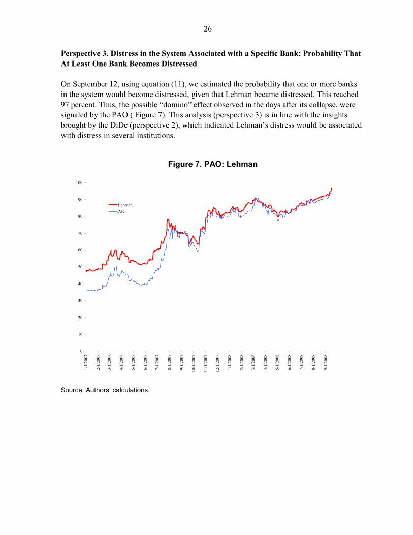
Perspective 3. Distress in the System Associated with a Specific Bank: Probability That At Least One Bank Becomes Distressed On September 12, using equation (11), we estimated the probability that one or more banks in the system would become distressed, given that Lehman became distressed. This reached 97 percent. Thus, the possible “domino” effect observed in the days after its collapse, were signaled by the PAO ( Figure 7). This analysis (perspective 3) is in line with the insights brought by the DiDe (perspective 2), which indicated Lehman’s distress would be associated with distress in several institutions.

Figure 7. PAO: Lehman

0

10

20

30

40

50

60

70

80

90

100

1/1/

2007

2/1/

2007

3/1/

2007

4/1/

2007

5/1/

2007

6/1/

2007

7/1/

2007

8/1/

2007

9/1/

2007

10/1

/200

7

11/1

/200

7

12/1

/200

7

1/1/

2008

2/1/

2008

3/1/

2008

4/1/

2008

5/1/

2008

6/1/

2008

7/1/

2008

8/1/

2008

9/1/

2008

LehmanAIG


27

C. Analysis of Cross-Region Effects Between Different Banking Groups

In order to gain insight into the cross region effects between American and European banking groups, we included five major European banks (Barclays and HSBC from the UK, UBS and Credit-Suisse (CSFB) from Switzerland, and Deutsche from Germany). Perspective 1. Common Distress in the Banks of the System: BSI and JPoD

• The JPoD indicates that risks among European banks are highly interconnected, with distress in one bank associated with a high probability of distress elsewhere in Europe. The European JPoD and BSI move in tandem with movements in the US indicators, coinciding also with relevant market events. (Figures 3 and 4).

• Distress dependence among banks in Europe also rises during times of crisis, indicating that systemic risks, as implied by the JPoD and the BSI rise faster than idiosyncratic risks. In Figure 5 it is clear that also for European banks, the daily percentage changes of the JPoD are larger than those of the individual (average) PoDs.

• Risks for European banks as measured by JPoD and the BSI appear lower than those for US IBs’ and very similar to those for US BHCs’ across time. Figures 3 and 4 also show that risks among European banks were similar at the time of the Bear Stearns debacle (March 17) and Lehman’s collapse (September 15). This is in contrast to American banks for which risks appear larger at the time of Lehman’s collapse. However, the situation in Europe appeared to be deteriorating fast in mid-September.

Perspective 2. Distress Between Specific Banks: Distress Dependence Matrix • Links across major European banks have increased significantly (Table 2). This is clearly

shown by the conditional PoDs presented in quadrant 4 of the DiDe matrices. On average, if any of the European banks appeared in distress, the probability of the other banks being distressed increased from 34 percent on July 17 , 2007 to 41 percent on September 12, 2008.

• Among the European banks under analysis, UBS appeared to be the bank under highest stress on September 12, 2008. It showed the largest PoD conditional on any other bank falling into distress, reaching on average 48 percent (row-average UBS). UBS’s distress would also be associated with high stress on Barclays, whose probability of distress conditional on UBS becoming distressed was estimated to reach 31 percent on September 12, 2008. This was a signifiant increase from 18 percent estimated on July 17, 2007.

• Among the European banks under analysis, distress at Credit Suisse (CSFB) would be associated with the highest stress on other European banks on September 12, 2008. The (average) PoD of European banks conditional on CSFB falling into distress reached 43 percent (quadrant 4, column-average CSFB). However, the European bank that would be

28

associated with the highest distress among American Banks is Deutsche. The (average) PoD of American banks conditional on Deutsche falling into distress reached 35 percent. (quadrant 2, column-average Deutsche). This might be related to the high integration of Deutsche in some markets at the global level.

• On September 12, 2008, while failure of one of the U.S. banks implied (on average) chances of distress of one European bank of 7 percent (quadrant 3), the (average) probability of distress of one American bank, conditional on a European bank becoming distressed is above 30 percent (quadrant 2). This is possibly because a European default would imply more generalized problems, including in U.S. markets.

Even though distress dependence does not imply causation, these results help explain why the Lehman bankruptcy led to a global crisis. The bankruptcy of Lehman appears to have sealed the fate of AIG and Washington Mutual, while putting greatly increased pressure on Wachovia, as indicated by the DiDe. In market terms, this was equivalent to the failure of a major U.S. institution, with significant reverberations on both sides of the Atlantic, as indicated by the ALPoD.

D. Analysis of Foreign Banks’ Risks to Sovereigns with Banking Systems with Cross-Border Institutions

We extend our methodology to analyze how rising problems in advanced country banking systems are linked with increasing risks to emerging markets. For this purpose, we use CDS spreads written on sovereign and banks’ bonds to derive probabilities of distress of banks and sovereigns. Therefore, such PoDs represent markets’ views of risks of distress for these banks and countries. While absolute risks are discussed, the focus is largely on cross distress dependence of risks and what they can say about emerging vulnerabilities (perspective 2). More precisely, using publicly available data we estimate cross vulnerabilities between Latin American, eastern European, and Asian emerging markets and the advanced country banks with larger regional presences in these regions. The countries and banks analyzed are: • Latin America. Countries: Mexico, Colombia, Brazil and Chile. Banks: BBVA,

Santander, Citigroup, Scotia Bank and HSBC. • Eastern Europe. Countries: Bulgaria, Croatia, Hungary and Slovakia. Banks: Intesa,

Unicredito, Erste, Societe Generale, and Citigroup. • Asia. Countries: China, Korea, Thailand, Malaysia, the Philippines, and Indonesia.

Banks: Citigroup, JP Morgan Chase, HSBC, Standard and Chartered, BNP, Deutsche, and DBS.

The key observation from the analysis is that concerns about bank solvency and emerging market instability appear to be highly interlinked. The markets’ evolving views of risks of distress for these banks and countries, based on market credit default swaps, are presented in Figure 8.

29

Table 2. Distress Dependence Matrix: American and European Banks

July 1, 2007 Citi BAC JPM Wacho WAMU GS LEH MER MS AIG Row average BARC HSBC UBS CSFB DB Row

averageCitigroup 1.00 0.14 0.11 0.11 0.08 0.09 0.08 0.09 0.09 0.08 0.19 Citigroup 0.07 0.07 0.08 0.06 0.07 0.07Bank of America 0.12 1.00 0.27 0.27 0.11 0.11 0.10 0.12 0.12 0.15 0.24 Bank of America 0.08 0.07 0.09 0.06 0.10 0.08JPMorgan 0.15 0.42 1.00 0.31 0.13 0.19 0.16 0.19 0.18 0.17 0.29 JPMorgan 0.10 0.08 0.12 0.09 0.14 0.10Wachovia 0.12 0.33 0.24 1.00 0.11 0.12 0.10 0.12 0.12 0.14 0.24 Wachovia 0.07 0.05 0.07 0.05 0.08 0.07Washington Mutual 0.16 0.28 0.21 0.23 1.00 0.12 0.12 0.16 0.13 0.15 0.26 Washington Mutual 0.09 0.08 0.09 0.06 0.09 0.08Goldman Sachs 0.17 0.25 0.28 0.21 0.11 1.00 0.31 0.28 0.31 0.17 0.31 Goldman Sachs 0.13 0.11 0.15 0.12 0.18 0.14Lehman 0.22 0.32 0.32 0.26 0.15 0.43 1.00 0.35 0.33 0.20 0.36 Lehman 0.14 0.12 0.15 0.14 0.22 0.15Merrill Lynch 0.19 0.32 0.33 0.25 0.17 0.33 0.31 1.00 0.31 0.20 0.34 Merrill Lynch 0.15 0.15 0.19 0.15 0.21 0.17Morgan Stanley 0.19 0.31 0.28 0.24 0.14 0.35 0.28 0.30 1.00 0.16 0.33 Morgan Stanley 0.14 0.12 0.14 0.12 0.18 0.14AIG 0.07 0.14 0.10 0.10 0.05 0.07 0.06 0.07 0.06 1.00 0.17 AIG 0.05 0.06 0.07 0.04 0.06 0.06Column average 0.24 0.35 0.31 0.30 0.21 0.28 0.25 0.27 0.26 0.24 0.27 Column average 0.10 0.09 0.11 0.09 0.13 0.11

Citi BAC JPM Wacho WAMU GS LEH MER MS AIG Row average BARC HSBC UBS CSFB DB Row

averageBarclay's 0.04 0.05 0.04 0.04 0.02 0.04 0.03 0.04 0.04 0.04 0.04 Barclay's 1.00 0.18 0.18 0.12 0.12 0.32HSBC 0.04 0.04 0.03 0.02 0.02 0.03 0.02 0.03 0.03 0.04 0.03 HSBC 0.16 1.00 0.13 0.09 0.11 0.30UBS 0.04 0.05 0.04 0.03 0.02 0.04 0.03 0.04 0.03 0.04 0.04 UBS 0.17 0.13 1.00 0.21 0.15 0.33CSFB 0.05 0.06 0.05 0.04 0.03 0.05 0.05 0.06 0.05 0.05 0.05 CSFB 0.19 0.15 0.36 1.00 0.21 0.38Deutsche Bank 0.05 0.09 0.08 0.06 0.03 0.07 0.06 0.07 0.06 0.06 0.06 Deutsche Bank 0.17 0.16 0.22 0.19 1.00 0.35Column average 0.05 0.06 0.05 0.04 0.02 0.05 0.04 0.05 0.04 0.05 0.04 Column average 0.34 0.32 0.38 0.32 0.32 0.34

September 12, 2008 Citi BAC JPM Wacho WAMU GS LEH MER MS AIG Row average BARC HSBC UBS CSFB DB Row

averageCitigroup 1.00 0.20 0.19 0.14 0.07 0.17 0.13 0.14 0.16 0.11 0.23 Citigroup 0.15 0.17 0.17 0.15 0.16 0.16Bank of America 0.14 1.00 0.31 0.18 0.05 0.16 0.10 0.13 0.15 0.11 0.23 Bank of America 0.12 0.13 0.13 0.11 0.15 0.13JPMorgan 0.13 0.29 1.00 0.16 0.05 0.19 0.11 0.14 0.16 0.09 0.23 JPMorgan 0.11 0.10 0.12 0.11 0.15 0.12Wachovia 0.34 0.60 0.55 1.00 0.17 0.36 0.27 0.31 0.34 0.29 0.42 Wachovia 0.27 0.23 0.27 0.25 0.31 0.27Washington Mutual 0.93 0.97 0.95 0.94 1.00 0.91 0.88 0.92 0.91 0.89 0.93 Washington Mutual 0.87 0.86 0.86 0.83 0.86 0.86Goldman Sachs 0.15 0.19 0.24 0.13 0.06 1.00 0.18 0.20 0.27 0.11 0.25 Goldman Sachs 0.14 0.13 0.15 0.15 0.19 0.15Lehman 0.47 0.53 0.58 0.43 0.25 0.75 1.00 0.59 0.62 0.37 0.56 Lehman 0.39 0.37 0.40 0.42 0.52 0.42Merrill Lynch 0.32 0.41 0.47 0.30 0.16 0.53 0.37 1.00 0.48 0.26 0.43 Merrill Lynch 0.31 0.33 0.35 0.35 0.39 0.35Morgan Stanley 0.21 0.28 0.29 0.19 0.09 0.40 0.22 0.27 1.00 0.14 0.31 Morgan Stanley 0.18 0.18 0.18 0.18 0.23 0.19AIG 0.50 0.66 0.59 0.53 0.29 0.54 0.43 0.49 0.47 1.00 0.55 AIG 0.49 0.53 0.53 0.49 0.53 0.52Column average 0.42 0.51 0.52 0.40 0.22 0.50 0.37 0.42 0.46 0.34 0.41 Column average 0.30 0.30 0.32 0.31 0.35 0.32

Citi BAC JPM Wacho WAMU GS LEH MER MS AIG Row average BARC HSBC UBS CSFB DB Row

averageBarclay's 0.10 0.11 0.10 0.08 0.04 0.10 0.07 0.09 0.09 0.07 0.08 Barclay's 1.00 0.36 0.31 0.30 0.28 0.45HSBC 0.06 0.06 0.05 0.03 0.02 0.05 0.04 0.05 0.05 0.04 0.05 HSBC 0.20 1.00 0.16 0.16 0.17 0.34UBS 0.11 0.11 0.11 0.07 0.04 0.11 0.07 0.10 0.09 0.08 0.09 UBS 0.32 0.30 1.00 0.47 0.34 0.48CSFB 0.07 0.07 0.07 0.05 0.03 0.07 0.05 0.07 0.06 0.05 0.06 CSFB 0.20 0.20 0.31 1.00 0.26 0.40Deutsche Bank 0.06 0.08 0.09 0.05 0.03 0.09 0.06 0.07 0.07 0.05 0.06 Deutsche Bank 0.18 0.20 0.21 0.24 1.00 0.36Column average 0.08 0.09 0.08 0.06 0.03 0.09 0.06 0.07 0.07 0.06 0.07 Column average 0.38 0.41 0.40 0.43 0.41 0.41

Source: Authors' calculations.1/ Probability of distress of the bank in the row, conditional on the bank in the column becoming distressed.

Distress Dependence Matrices, July 2007 and September 2008 1/

30

The level of risk in Latin America and Asia was falling in the run-up to the crisis, and was about to converge with the low level of concern about advanced country banks and Eastern Europe. However, since August 2008, both sovereign risk and bank risk have risen sharply and moved increasingly in tandem. This points to close interlinkages between concerns about bank solvency and emerging market instability. Perspective 2. Distress between specific banks: distress dependence matrix To gain insight into these interlinkages and how they have evolved, in Tables 3, 4, and 5, we present the DiDe matrices estimated for Latin America, eastern Europe and Asia respectively. We have chosen July 1, 2007, and September 16, 2008; thus, we can show how conditional probabilities of distress have changed from a pre-crisis period to the post-Lehman episode. The DiDe matrices report probabilities that a bank/country in a row will become distressed if the bank/country in the column fails. Most importantly, as well as links across countries (bottom right, quadrant 4) and across banks (top left, quadrant 1) they report cross dependencies between these groups. The bottom left (quadrant 3) reports how bank problems can presage sovereign distress, while the top right (quadrant 2) indicates the opposite link. As noted above, while dependence does not imply causation, such correlations provide important insights. In particular:

• Cross dependencies have risen sharply over the crisis, implying that systemic risks have leapt. This is clearly seen when comparing the probability of distress of the sovereigns conditional on distress on the banks between July 2007, when sovereigns appeared to have low risk of contamination, and September 2008. For Latin America, the average conditional PoD increased from 39 to 51 percent, for eastern Europe from 16 to 46 percent and for Asia, from 12 to 34 percent (quadrant 3). The increase in the probability of distress of the banks, conditional on distress of the sovereigns, is even more significant, as eroding capital has increased exposure. For Latin America, the average conditional PoD of the relevant banks increased from 13 to 54 percent, for eastern Europe from 11 to 45 percent and for Asia, from 4 to 30 percent (quadrant 2).

• Of particular interest is to see how bank problems can presage sovereign distress. We can see that before the crisis, the conditional probabilities of distress for Chile and Mexico were the lowest in Latin America (quadrant 3, row-average); however, on September 16, 2008, there was a significant increase for Mexico, making it the country with the second highest conditional PoD in its region. Chile also recorded an increase, although it still remains the country with the lowest conditional PoD in its region. In eastern Europe, on September 16, our model was already signaling that Bulgaria and Hungary were under significant stress. In Asia, Indonesia, Korea, and the Phillipines were at highest risk. However Slovakia and China remained the least stressed in those regions (quadrant 3, row-average).

• Country distress conditional on bank distress appears high (quadrant 3). Distress of Spanish banks would be associated with the highest distress in Latin America and Italian

31

banks in eastern Europe. Distress of Standard Chartered would be associated with significant stress in Asia (quadrant 3, column-average). These results suggest that geographic roles matter, since these banks have a substantial presence in the respective regions under analysis.

• Moreover, these banks seem less dependent than others on country risks (quadrant 2, row-average). This seemingly paradoxical pattern is likely because the Spanish/Italian banks are seen as relatively safe, and hence their distress would signal larger systemic financial problems that would feed through to emerging markets in which they have a large presence.

• Vulnerabilities between countries (quadrant 4) were highest in Brazil, Mexico, Bulgaria Hungary, Indonesia, Phillipines, and Korea (quadrant 4, row-average). Vulnerabilities between banks (quadrant 1) were highest for Citi, Scotia, Erste (quadrant 1, row-average).

• Direct links between banks and countries matter. Distress in countries with a particularly large foreign bank presence—such as Mexico and Croatia—is highly linked with potential banking distress (quadrant 2). At a more specific level, direct links from individual banks to countries also matter—for example, distress at Citigroup, Intesa, and DBS are relatively more important for Mexico, Hungary, and Indonesia, respectively, than for other countries (quadrant 3).

• These results also illustrate how the leap in systemic risk, and hence indirect links, has affected Asia, over and above direct regional and bilateral ties. This is because direct ownership and lending by foreign banks is generally lower in Asia than in eastern Europe or Latin America. Since the banking systems are more insulated from these direct links, the results are more likely to reflect indirect ones through overall risks linked to bank/sovereign distress. In addition, links between banks may be somewhat less important for emerging Asia, as borrowing through equity markets tends to play a larger role in local financial markets. Thus, powerful indirect effects appear evident in all cases, particularly for Korea and Indonesia.

• An important strength of our approach is that market prices reflect perceptions of direct links and indirect links. For the former, market presence might be an important element, as in Latin America and eastern Europe; however, for the latter, liquidity pressures and systemic banking distress/macroeconomic spillovers might play an important role. This feature of our approach appears to be particularly relevant in Asia.

The results confirm that systemic bank risks and emerging market vulnerabilities are highly dependent. This likely largely reflects the fact that distress in individual banks is a bellweather for the state of the overall financial system, via direct or indirect links. In financial terms, the world is increasingly a global village. The bottom line is that policies to limit systemic risks in advanced country financial systems would also sharply reduce risks to emerging markets.

32

Figure 8. Foreign-Bank and Sovereign Risks

Eastern Europe

0.00

0.00

0.01

0.01

0.02

0.02

1/2/2005 7/2/2005 1/2/2006 7/2/2006 1/2/2007 7/2/2007 1/2/2008 7/2/2008

Bank AverageSovereign Average

Latin America

0.00

0.01

0.01

0.02

0.02

0.03

1/2/2005 7/2/2005 1/2/2006 7/2/2006 1/2/2007 7/2/2007 1/2/2008 7/2/2008


Emerging Asia

0.00

0.01

0.01

0.02

0.02

0.03

0.03

1/2/2005 7/2/2005 1/2/2006 7/2/2006 1/2/2007 7/2/2007 1/2/2008 7/2/2008



33

Table 3. Distress Dependence Matrix: Latin America. Sovereigns And Banks

7/1/2007 BBVA SAN CITI SCOTIA HSBC Row Average MEXICO COLOMBIA BRAZIL CHILE Row Average

BBVA 1.00 0.54 0.17 0.12 0.38 0.44 BBVA 0.13 0.08 0.08 0.23 0.13SANTANDER 0.57 1.00 0.15 0.13 0.37 0.44 SANTANDER 0.14 0.08 0.09 0.24 0.14

CITI 0.18 0.16 1.00 0.21 0.18 0.34 CITI 0.14 0.05 0.08 0.15 0.10SCOTIA 0.23 0.23 0.36 1.00 0.23 0.41 SCOTIA 0.22 0.10 0.13 0.23 0.17HSBC 0.36 0.33 0.15 0.12 1.00 0.39 HSBC 0.12 0.07 0.07 0.19 0.11

Column Average 0.47 0.45 0.37 0.32 0.43 0.41 Column Average 0.15 0.07 0.09 0.21 0.13

BBVA SAN CITI SCOTIA HSBC Row Average MEXICO COLOMBIA BRAZIL CHILE Row Average

MEXICO 0.39 0.41 0.40 0.35 0.38 0.39 MEXICO 1.00 0.18 0.32 0.57 0.52COLOMBIA 0.54 0.54 0.33 0.38 0.51 0.46 COLOMBIA 0.43 1.00 0.34 0.59 0.59

BRAZIL 0.52 0.56 0.47 0.44 0.48 0.49 BRAZIL 0.68 0.31 1.00 0.69 0.67CHILE 0.25 0.26 0.16 0.14 0.23 0.21 CHILE 0.21 0.09 0.12 1.00 0.36


9/16/2008 BBVA SAN CITI SCOTIA HSBC Row Average MEXICO COLOMBIA BRAZIL CHILE Row Average

BBVA 1.00 0.79 0.42 0.38 0.69 0.66 BBVA 0.47 0.39 0.42 0.61 0.47SANTANDER 0.77 1.00 0.39 0.36 0.66 0.64 SANTANDER 0.46 0.38 0.42 0.62 0.47

CITI 0.75 0.73 1.00 0.68 0.75 0.78 CITI 0.73 0.53 0.63 0.75 0.66SCOTIA 0.79 0.79 0.80 1.00 0.80 0.84 SCOTIA 0.80 0.63 0.71 0.82 0.74HSBC 0.54 0.53 0.33 0.30 1.00 0.54 HSBC 0.36 0.29 0.30 0.41 0.34


BBVA SAN CITI SCOTIA HSBC Row Average MEXICO COLOMBIA BRAZIL CHILE Row Average

MEXICO 0.61 0.62 0.53 0.49 0.60 0.57 MEXICO 1.00 0.46 0.64 0.76 0.71COLOMBIA 0.66 0.67 0.50 0.51 0.64 0.60 COLOMBIA 0.61 1.00 0.57 0.72 0.72

BRAZIL 0.61 0.63 0.52 0.50 0.57 0.57 BRAZIL 0.72 0.49 1.00 0.72 0.73CHILE 0.35 0.37 0.24 0.22 0.30 0.30 CHILE 0.34 0.24 0.28 1.00 0.47


Source: Authors' calculationsThese matrices present the probability of distress of the bank/sovereign in the row, conditional on the bank/sovereign in the column.

34

Table 4. Distress Dependence Matrix: Eastern Europe. Sovereigns And Banks

7/1/2007 INTESA UNICREDITO ERSTE SOCIETE CITI Row Average BULGARIA CROATIA HUNGARY SLOVAKIA Row Average

INTESA 1.00 0.37 0.20 0.29 0.12 0.40 INTESA 0.06 0.12 0.15 0.09 0.11UNICREDITO 0.49 1.00 0.25 0.40 0.16 0.46 UNICREDITO 0.07 0.15 0.18 0.10 0.13

ERSTE 0.31 0.30 1.00 0.32 0.14 0.41 ERSTE 0.09 0.16 0.22 0.09 0.14SOCIETE 0.30 0.32 0.21 1.00 0.13 0.39 SOCIETE 0.07 0.10 0.13 0.09 0.10

CITI 0.19 0.19 0.14 0.20 1.00 0.34 CITI 0.05 0.09 0.12 0.09 0.09Column Average 0.46 0.43 0.36 0.44 0.31 0.40 Column Average 0.07 0.12 0.16 0.09 0.11

INTESA UNICREDITO ERSTE SOCIETE CITI Row Average BULGARIA CROATIA HUNGARY SLOVAKIA Row Average

BULGARIA 0.10 0.09 0.10 0.11 0.06 0.09 BULGARIA 1.00 0.15 0.09 0.11 0.34CROATIA 0.22 0.20 0.18 0.18 0.11 0.18 CROATIA 0.17 1.00 0.15 0.13 0.36

HUNGARY 0.36 0.32 0.33 0.29 0.18 0.30 HUNGARY 0.12 0.19 1.00 0.15 0.37SLOVAKIA 0.07 0.06 0.04 0.06 0.04 0.06 SLOVAKIA 0.05 0.05 0.05 1.00 0.29


9/16/2008 INTESA UNICREDITO ERSTE SOCIETE CITI Row Average BULGARIA CROATIA HUNGARY SLOVAKIA Row Average

INTESA 1.00 0.52 0.40 0.53 0.25 0.54 INTESA 0.17 0.26 0.35 0.30 0.27UNICREDITO 0.66 1.00 0.48 0.64 0.31 0.62 UNICREDITO 0.21 0.32 0.41 0.34 0.32

ERSTE 0.52 0.49 1.00 0.55 0.28 0.57 ERSTE 0.22 0.32 0.43 0.30 0.32SOCIETE 0.46 0.44 0.37 1.00 0.23 0.50 SOCIETE 0.17 0.22 0.28 0.27 0.24

CITI 0.52 0.51 0.45 0.55 1.00 0.61 CITI 0.24 0.33 0.41 0.38 0.34

INTESA UNICREDITO ERSTE SOCIETE CITI Row Average BULGARIA CROATIA HUNGARY SLOVAKIA Row Average

BULGARIA 0.34 0.32 0.33 0.37 0.22 0.32 BULGARIA 1.00 0.39 0.30 0.39 0.52CROATIA 0.47 0.44 0.44 0.45 0.28 0.42 CROATIA 0.36 1.00 0.38 0.38 0.53

HUNGARY 0.45 0.42 0.43 0.43 0.26 0.40 HUNGARY 0.20 0.28 1.00 0.31 0.45SLOVAKIA 0.13 0.12 0.10 0.14 0.08 0.12 SLOVAKIA 0.09 0.10 0.11 1.00 0.32



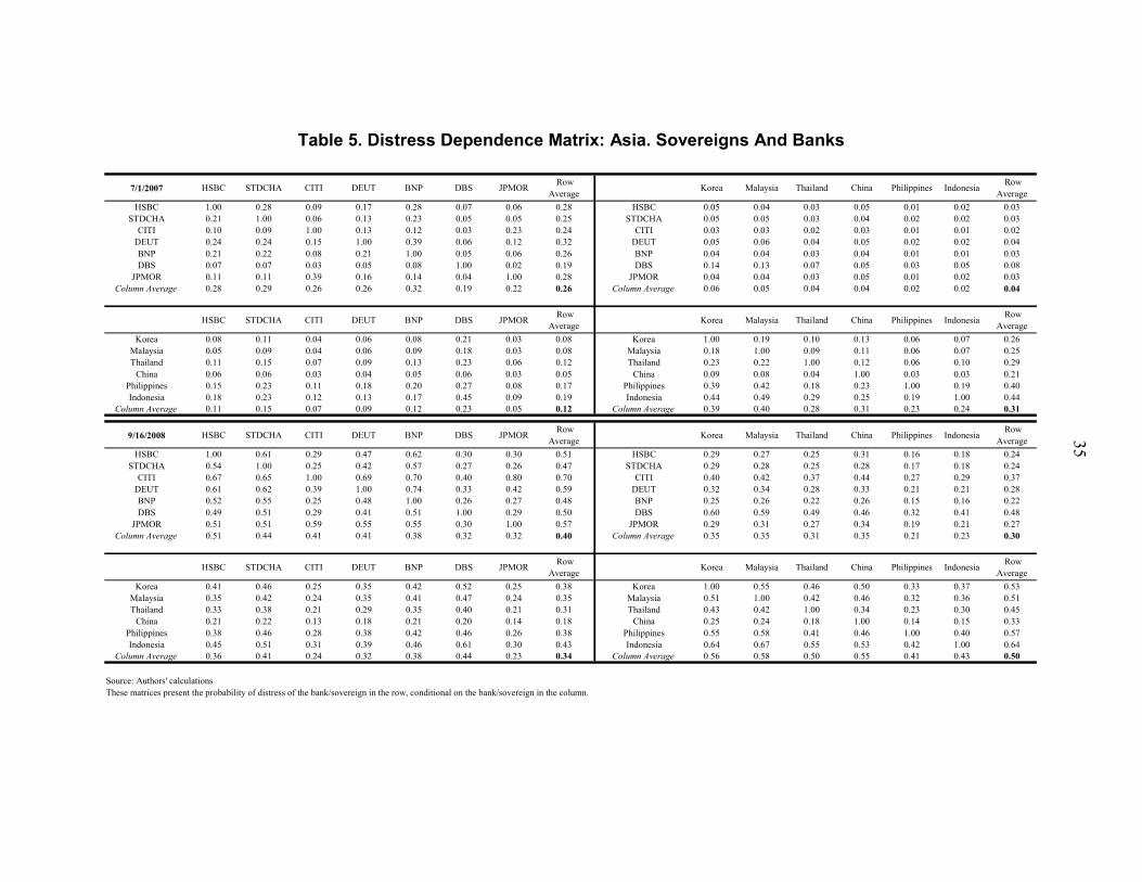
35

Table 5. Distress Dependence Matrix: Asia. Sovereigns And Banks

7/1/2007 HSBC STDCHA CITI DEUT BNP DBS JPMOR Row Average Korea Malaysia Thailand China Philippines Indonesia Row

AverageHSBC 1.00 0.28 0.09 0.17 0.28 0.07 0.06 0.28 HSBC 0.05 0.04 0.03 0.05 0.01 0.02 0.03

STDCHA 0.21 1.00 0.06 0.13 0.23 0.05 0.05 0.25 STDCHA 0.05 0.05 0.03 0.04 0.02 0.02 0.03CITI 0.10 0.09 1.00 0.13 0.12 0.03 0.23 0.24 CITI 0.03 0.03 0.02 0.03 0.01 0.01 0.02

DEUT 0.24 0.24 0.15 1.00 0.39 0.06 0.12 0.32 DEUT 0.05 0.06 0.04 0.05 0.02 0.02 0.04BNP 0.21 0.22 0.08 0.21 1.00 0.05 0.06 0.26 BNP 0.04 0.04 0.03 0.04 0.01 0.01 0.03DBS 0.07 0.07 0.03 0.05 0.08 1.00 0.02 0.19 DBS 0.14 0.13 0.07 0.05 0.03 0.05 0.08

JPMOR 0.11 0.11 0.39 0.16 0.14 0.04 1.00 0.28 JPMOR 0.04 0.04 0.03 0.05 0.01 0.02 0.03Column Average 0.28 0.29 0.26 0.26 0.32 0.19 0.22 0.26 Column Average 0.06 0.05 0.04 0.04 0.02 0.02 0.04

HSBC STDCHA CITI DEUT BNP DBS JPMOR Row Average Korea Malaysia Thailand China Philippines Indonesia Row

AverageKorea 0.08 0.11 0.04 0.06 0.08 0.21 0.03 0.08 Korea 1.00 0.19 0.10 0.13 0.06 0.07 0.26

Malaysia 0.05 0.09 0.04 0.06 0.09 0.18 0.03 0.08 Malaysia 0.18 1.00 0.09 0.11 0.06 0.07 0.25Thailand 0.11 0.15 0.07 0.09 0.13 0.23 0.06 0.12 Thailand 0.23 0.22 1.00 0.12 0.06 0.10 0.29

China 0.06 0.06 0.03 0.04 0.05 0.06 0.03 0.05 China 0.09 0.08 0.04 1.00 0.03 0.03 0.21Philippines 0.15 0.23 0.11 0.18 0.20 0.27 0.08 0.17 Philippines 0.39 0.42 0.18 0.23 1.00 0.19 0.40Indonesia 0.18 0.23 0.12 0.13 0.17 0.45 0.09 0.19 Indonesia 0.44 0.49 0.29 0.25 0.19 1.00 0.44

Column Average 0.11 0.15 0.07 0.09 0.12 0.23 0.05 0.12 Column Average 0.39 0.40 0.28 0.31 0.23 0.24 0.31

9/16/2008 HSBC STDCHA CITI DEUT BNP DBS JPMOR Row Average Korea Malaysia Thailand China Philippines Indonesia Row

AverageHSBC 1.00 0.61 0.29 0.47 0.62 0.30 0.30 0.51 HSBC 0.29 0.27 0.25 0.31 0.16 0.18 0.24

STDCHA 0.54 1.00 0.25 0.42 0.57 0.27 0.26 0.47 STDCHA 0.29 0.28 0.25 0.28 0.17 0.18 0.24CITI 0.67 0.65 1.00 0.69 0.70 0.40 0.80 0.70 CITI 0.40 0.42 0.37 0.44 0.27 0.29 0.37

DEUT 0.61 0.62 0.39 1.00 0.74 0.33 0.42 0.59 DEUT 0.32 0.34 0.28 0.33 0.21 0.21 0.28BNP 0.52 0.55 0.25 0.48 1.00 0.26 0.27 0.48 BNP 0.25 0.26 0.22 0.26 0.15 0.16 0.22DBS 0.49 0.51 0.29 0.41 0.51 1.00 0.29 0.50 DBS 0.60 0.59 0.49 0.46 0.32 0.41 0.48

JPMOR 0.51 0.51 0.59 0.55 0.55 0.30 1.00 0.57 JPMOR 0.29 0.31 0.27 0.34 0.19 0.21 0.27Column Average 0.51 0.44 0.41 0.41 0.38 0.32 0.32 0.40 Column Average 0.35 0.35 0.31 0.35 0.21 0.23 0.30

HSBC STDCHA CITI DEUT BNP DBS JPMOR Row Average Korea Malaysia Thailand China Philippines Indonesia Row

AverageKorea 0.41 0.46 0.25 0.35 0.42 0.52 0.25 0.38 Korea 1.00 0.55 0.46 0.50 0.33 0.37 0.53

Malaysia 0.35 0.42 0.24 0.35 0.41 0.47 0.24 0.35 Malaysia 0.51 1.00 0.42 0.46 0.32 0.36 0.51Thailand 0.33 0.38 0.21 0.29 0.35 0.40 0.21 0.31 Thailand 0.43 0.42 1.00 0.34 0.23 0.30 0.45

China 0.21 0.22 0.13 0.18 0.21 0.20 0.14 0.18 China 0.25 0.24 0.18 1.00 0.14 0.15 0.33Philippines 0.38 0.46 0.28 0.38 0.42 0.46 0.26 0.38 Philippines 0.55 0.58 0.41 0.46 1.00 0.40 0.57Indonesia 0.45 0.51 0.31 0.39 0.46 0.61 0.30 0.43 Indonesia 0.64 0.67 0.55 0.53 0.42 1.00 0.64

Column Average 0.36 0.41 0.24 0.32 0.38 0.44 0.23 0.34 Column Average 0.56 0.58 0.50 0.55 0.41 0.43 0.50


36

VI. CONCLUSIONS

The purpose of this paper is to seek to provide a set of quantitative measures of the financial stability of the main banks in any country, or region, so that this portfolio of banks’ relative stability as a group can be tracked over time and compared in a cross-section of comparative groupings. To this end we have developed a new framework that has several advantages. • It provides measures that allow us to analyze (define) stability from three different,

yet, complementary perspectives.

• It can be constructed from a very limited set of data, i.e., the empirical measurements of default probabilities of individual banks. Such measurements can be estimated using alternative approaches, depending on data availability; thus, the data set that is necessary for the estimation is available in many countries, both developed and developing, as long as there is reasonable data to reflect individual banks’ PoDs.

• It embeds the banks’ default interdependence structure (copula function), which captures linear and non-linear default dependencies among the main banks in a system.

• It allows the quantification of changes in the banks’ default interdependence structure at specific points in time; hence, it can be useful to quantify the empirically observed increases in dependencies in periods of distress, and relax the commonly used assumption in risk measurement models of fixed correlations across time.

The empirical part of the paper applied this methodology to a number of country and regional examples using publicly available information up to October 2008. This implementation flexibility is of relevance for banking stability surveillance, since cross-border financial linkages are growing and becoming significant, as has been highlighted by the financial market turmoil of recent months. Thus, surveillance of banking stability cannot stop at national borders. The proposed measures will allow us to complement our previous research and expand our research agenda; thus, we hope to gain further insights in our understanding of financial stability. For example, by tryiun to predict future movements of the BSMs for use as an early-warning mechanism; exploring the significant macroeconomic and financial factors and shocks influencing the BSMs, in order to identify macro-financial linkages; and exploring the factors that can limit and reverse tendencies towards instability, so as to discover what instruments may be available (and under what conditions) to control such instability.

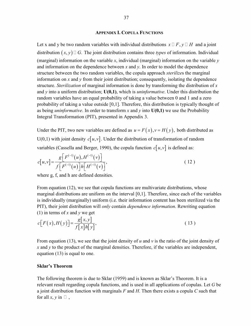
37

APPENDIX I. COPULA FUNCTIONS Let x and y be two random variables with individual distributions ,x F y H and a joint distribution ( ), .x y G The joint distribution contains three types of information. Individual (marginal) information on the variable x, individual (marginal) information on the variable y and information on the dependence between x and y. In order to model the dependence structure between the two random variables, the copula approach sterilizes the marginal information on x and y from their joint distribution; consequently, isolating the dependence structure. Sterilization of marginal information is done by transforming the distribution of x and y into a uniform distribution; U(0,1), which is uninformative. Under this distribution the random variables have an equal probability of taking a value between 0 and 1 and a zero probability of taking a value outside [0,1]. Therefore, this distribution is typically thought of as being uninformative. In order to transform x and y into U(0,1) we use the Probability Integral Transformation (PIT), presented in Appendix 3. Under the PIT, two new variables are defined as ( ) ( ), ,u F x v H y= = both distributed as

U(0,1) with joint density [ ],c u v . Under the distribution of transformation of random

variables (Cassella and Berger, 1990), the copula function [ ],c u v is defined as:

[ ]( ) ( ) ( ) ( )

( ) ( ) ( ) ( )

1 1

1 1

,, ,

g F u H vc u v

f F u h H v

− −

− −

⎡ ⎤⎣ ⎦=

⎡ ⎤ ⎡ ⎤⎣ ⎦ ⎣ ⎦

( 12 )

where g, f, and h are defined densities. From equation (12), we see that copula functions are multivariate distributions, whose marginal distributions are uniform on the interval [0,1]. Therefore, since each of the variables is individually (marginally) uniform (i.e. their information content has been sterilized via the PIT), their joint distribution will only contain dependence information. Rewriting equation (1) in terms of x and y we get

( ) ( ) [ ][ ] [ ]

,, ,

g x yc F x H y

f x h y=⎡ ⎤⎣ ⎦ ( 13 )

From equation (13), we see that the joint density of u and v is the ratio of the joint density of x and y to the product of the marginal densities. Therefore, if the variables are independent, equation (13) is equal to one. Sklar’s Theorem The following theorem is due to Sklar (1959) and is known as Sklar’s Theorem. It is a relevant result regarding copula functions, and is used in all applications of copulas. Let G be a joint distribution function with marginals F and H. Then there exists a copula C such that for all x, y in ,

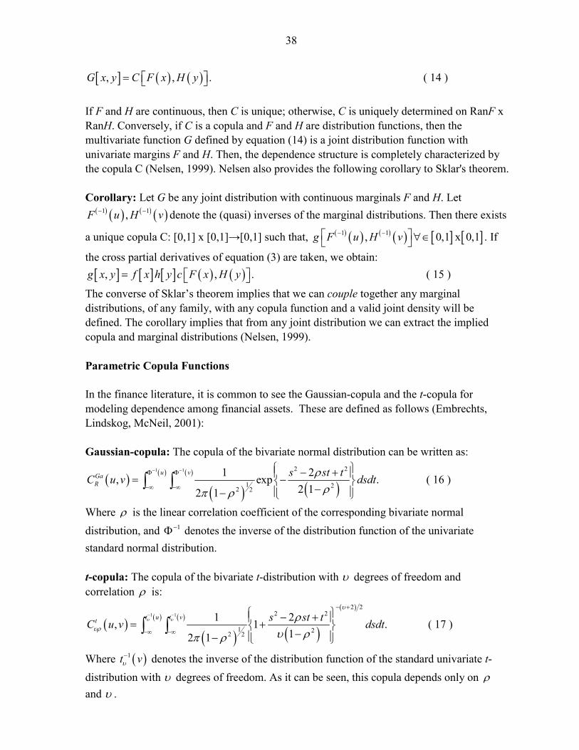
38

[ ] ( ) ( ), , .G x y C F x H y= ⎡ ⎤⎣ ⎦ ( 14 )

If F and H are continuous, then C is unique; otherwise, C is uniquely determined on RanF x RanH. Conversely, if C is a copula and F and H are distribution functions, then the multivariate function G defined by equation (14) is a joint distribution function with univariate margins F and H. Then, the dependence structure is completely characterized by the copula C (Nelsen, 1999). Nelsen also provides the following corollary to Sklar's theorem. Corollary: Let G be any joint distribution with continuous marginals F and H. Let

( ) ( ) ( ) ( )1 1,F u H v− − denote the (quasi) inverses of the marginal distributions. Then there exists

a unique copula C: [0,1] x [0,1]→[0,1] such that, ( ) ( ) ( ) ( ) [ ]1 1, 0,1g F u H v− −⎡ ⎤∀∈⎣ ⎦ x[ ]0,1 . If

the cross partial derivatives of equation (3) are taken, we obtain: [ ] [ ] [ ] ( ) ( ), , .g x y f x h y c F x H y= ⎡ ⎤⎣ ⎦ ( 15 )

The converse of Sklar’s theorem implies that we can couple together any marginal distributions, of any family, with any copula function and a valid joint density will be defined. The corollary implies that from any joint distribution we can extract the implied copula and marginal distributions (Nelsen, 1999). Parametric Copula Functions In the finance literature, it is common to see the Gaussian-copula and the t-copula for modeling dependence among financial assets. These are defined as follows (Embrechts, Lindskog, McNeil, 2001): Gaussian-copula: The copula of the bivariate normal distribution can be written as:

( )( )

( )( )

( )1 1 2 2

1 22 2

1 2, exp .2 12 1

u vGaR

s st tC u v dsdtρρπ ρ

− −Φ Φ

−∞ −∞

⎧ ⎫− +⎪ ⎪= −⎨ ⎬−⎪ ⎪− ⎩ ⎭

∫ ∫ ( 16 )

Where ρ is the linear correlation coefficient of the corresponding bivariate normal distribution, and 1−Φ denotes the inverse of the distribution function of the univariate standard normal distribution. t-copula: The copula of the bivariate t-distribution with υ degrees of freedom and correlation ρ is:

( )( )

( )( )

( )

( )1 1

2 22 2

1 22 2

1 2, 1 .12 1

t u t vt s st tC u v dsdtυ υ

υ

υρρ

υ ρπ ρ

− −− +

−∞ −∞

⎧ ⎫− +⎪ ⎪= +⎨ ⎬−⎪ ⎪− ⎩ ⎭

∫ ∫ ( 17 )

Where ( )1t vυ− denotes the inverse of the distribution function of the standard univariate t-

distribution with υ degrees of freedom. As it can be seen, this copula depends only on ρ and υ .

39

APPENDIX II. CIMDO-COPULA In order to provide a heuristic explanation of the CIMDO-copula, we compare the copula of a bivariate CIMDO-distribution and a bivariate distribution of the form that the prior density in the entropy functional would be set; e.g., a t-distribution. First, we recall from equation (1) that copula functions were defined as

[ ]( ) ( ) ( ) ( )

( ) ( ) ( ) ( )

1 1

1 1

,, .

g F u H vc u v

f F u h H v

− −

− −

⎡ ⎤⎣ ⎦=

⎡ ⎤ ⎡ ⎤⎣ ⎦ ⎣ ⎦

Assume that the prior has a density function ( ),q x y . Hence, its marginal cumulative

distribution functions are of the form, ( ) ( , )x

u F x q x y dydx+∞

−∞ −∞= = ∫ ∫ , and

( ) ( , )x

v H y q x y dxdy+∞

−∞ −∞= = ∫ ∫ ; where 1( ) ( ),u F x x F u−= ⇔ = and 1( ) ( ).v H y y H v−= ⇔ =

Therefore, its marginal densities are of the form, ( ) ( , ) ,f x q x y dy+∞

−∞= ∫ and

( ) ( , ) .h y q x y dx+∞

−∞= ∫

Substituting these into the copula definition we get, the copula of the prior, ( , )qc u v , 1 1

1 1

( ), ( )( , )

( ), , ( )q

q F u H vc u v

q F u y dy q x H v dx

− −

+∞ +∞− −

−∞ −∞

⎡ ⎤⎣ ⎦=⎡ ⎤ ⎡ ⎤⎣ ⎦ ⎣ ⎦∫ ∫

. ( 18 )

Similarly, assume that the CIMDO distribution with q(x,y) as the prior is of the form,

) )1 2, ,( , ) ( , ) exp 1 ( ) ( ) .x y

d dx xp x y q x y μ λ χ λ χ⎡ ⎡∞ ∞⎣ ⎣

⎧ ⎫⎡ ⎤= − + + +⎨ ⎬⎢ ⎥⎣ ⎦⎩ ⎭ We also define

1( ) ( ),c cu F x x F u−= ⇔ = and 1( ) ( ).c cv H y y H v−= ⇔ = Its marginal densities take the form,

( ) ( ){ }1 2( ) ( , ) exp 1 ( ) ( ) ,x yd d

c x xf x q x y x y dyμ λ χ λ χ

+∞

−∞⎡ ⎤= − + + +⎣ ⎦∫ and

( ) ( ){ }1 2( ) ( , ) exp 1 ( ) ( ) .x yd d

c x xh y q x y x y dxμ λ χ λ χ

+∞

−∞⎡ ⎤= − + + +⎣ ⎦∫

Substituting these into the copula definition we get, the CIMDO-copula, ( , ),cc u v

{ }( ){ } ( ){ }

1 1

1 12 1

( ), ( ) exp 1( , )

( ), exp , ( ) expy xdd

c c

c

c c xx

q F u H vc u v

q F u y y dy q x H v x dx

μ

λ χ λ χ

− −

+∞ +∞− −

−∞ −∞

⎡ ⎤⎡ ⎤ − +⎣ ⎦ ⎣ ⎦=⎡ ⎤ ⎡ ⎤− −⎣ ⎦ ⎣ ⎦∫ ∫

. ( 19 )

Equation (14) shows that the CIMDO-copula is a nonlinear function of 1 2, , andμ λ λ , which change as the PoDs of the banks under analysis change. Therefore, the CIMDO-copula captures changes in PoDs, as these change at different periods of the economic cycle.

40

APPENDIX III. CIMDO-DENSITY AND CIMDO-COPULA EVALUATION FRAMEWORK We consider extremely important the evaluation framework used to assess whether CIMDO-distributions and CIMDO-copulas provide improvements over the most commonly parametric distributions, copulas used for portfolio credit risk modeling. In order to evaluate these densities, we follow the Probability Integral Transformation approach (PIT) developed by Diebold et al (1999). In what follows in this section, we provide a summary of the detailed theoretical results supporting the chosen evaluation criterion. A complete development and Monte Carlo exercise can be found in (Segoviano 2006b). The Probability Integral Transformation Approach (PIT) Density evaluation is not a trivial problem, since there is no way to rank two incorrect density forecasts such that all users will agree with the ranking. Ranking depends on the specific loss functions of the users.14 However, Diebold et al. (1998) assert that if a forecast coincides with a random variable true data generating process (DGP), then it will be preferred by all forecast users, regardless of loss function. Thus this proposition implies that, regardless of the users’ loss function, the correct density is weakly superior to all forecasts. As a result, Diebold et al. (1998) suggest evaluating forecasts by assessing whether the forecast densities are correct; i.e., by assessing whether the forecast coincide with the true DGP. Nonetheless, the task of determining whether a forecast equals the true DGP appears to be difficult because the true DGP is never observed. Moreover, the true density may exhibit structural changes at every point in time. To overcome this difficulty, they developed a method based on the Rosenblatt (1952) Probability Integral Transformation (PIT). Diebold et al. (1998) prove that the series of the Probability Integral Transformations of a series of density forecasts are distributed iid U(0,1) if the density forecasts coincide with the true DGP. Thus, to assess whether a series of density forecasts coincides with the corresponding series of true conditional densities, it is only necessary to test whether the sequence of density forecast PITs are iid U(0,1). Diebold, Hahn, and Tay (1999) extend their results to the Mth-multivariate case. Suppose there is a series of T, Mth-multivariate density forecasts. They factorize each period’s t, joint forecast density into the product of their conditionals:15

1 1 1 2 1 11 1 1 1( ,.., ) ( | ,.. ).. ( | ) ( ).M M M

t t t t t t t t t t t tp l l p l l l p l l p l−− − − −= ⋅ ⋅

This procedure produces a set of (M-1) conditionals and (1) marginal density. The PIT's of the lm random variable realizations under these M series will be iid U(0,1), individually and also 14The result is analogous to Arrow's celebrated impossibility theorem. The ranking effectively reflects a social welfare function, which does not exist.

41

when taken as a whole, if the multivariate density forecasts are correct. The proof of this assertion in a time series framework can be found in Diebold et al. (1999). CIMDO: Density Evaluation However, we needed to develop a slightly different test. This is because CIMDO recovers densities with information at each period of time t.16 Thus, the density evaluation needs to be done at specific periods of time t. Alternatively, rather than evaluating a time-series as Diebold et al (1999) do, we would like to evaluate cross-sectionally the multivariate distribution. As a result, we need to prove that at each point in time t, the product of the conditionals and marginal PIT's on which a multivariate distribution can be decomposed is iid U(0,1).This proof is not explicitly presented in Diebold et al (1999); therefore, we develop the proof in Segoviano (2006b) In the interest of parsimony, we focus on a portfolio containing two different types of assets (e.g., types of loans or in the case of this paper, two different banks), whose logarithmic returns are characterized by the random variables x and y, where , , ix y l∈ s.t. 1,.., .i M= The portfolio bivariate density can be decomposed into,

( , ) ( ) ( | ),p x y p x p y x= ⋅ ( 20 ) ( , ) ( ) ( | ).p x y p y p x y= ⋅ ( 21 )

We start by analyzing the first case presented in equation (20). Under the PIT, two new variables are defined as

( 1)

( 1)

( ) ( ),( | ) ( | ).

u P x x P uv P y x y P v x

−

−

= ⇔ =

= ⇔ =

First we prove that u,v are distributed iid U(0,1) then we prove that they are independent. Uniform Distribution Proof Based on the PIT, we present the distributional proof. Theorem: Probability Integral Transformation Let x be a random vector with absolute continuous cumulative density function (cdf) F. Define a new random variable, the Probability Integral Transformation (PIT) as,

( ).U F x= Then, ( , )U ∼ U 0 1 regardless of the original distribution F. Note that in this case, ( )U F x=

is a generalization of ( )u P x= and ( / ).v P y x=

15Note that the Mth multivariate density can be factorized into M! ways at each period of time t. 16 Recall that the CIMDO- density is re-estimated at each period of time; i.e., it updates period by period.

42

Proof. ( , )U ∼ U 0 1 For u on [ ]0,1 , we have:

[ ] [ ]( )P U u P F x u≤ = ≤

[ ] ( )1 1( )P F F x F u− −⎡ ⎤= ≤⎣ ⎦

( )1P x F u−⎡ ⎤= ≤⎣ ⎦

( )1F F u−⎡ ⎤= ⎣ ⎦

u= For 0,u < [ ] 0P U u< = and for 1u > , [ ] 0P U u> = since the range of a cdf is [ ]0,1 . Independence Proof Proposition. ,u v are independent. Proof. In order to prove the independence assumption, we know that the joint density [ ],c u v is defined under the distribution of transformations of random variables as (Cassella and Berger, 1990),

[ ] ( 1) ( 1), ( ), ( | ) .x xu vy yu v

c u v p P u P v x∂ ∂∂ ∂− −∂ ∂∂ ∂

⎡ ⎤= ⋅⎣ ⎦

Since in this case 1( 1) ( 1)

1( 1) ( 1)

( ) ( ) ( ) ,

( | ) ( | ) ( | ) | ,

0,

xu P x x P u p P uu

yv P y x y P v x p P v x xv

x yv u

−− −

−− −

∂ ⎡ ⎤= ⇔ = ⇒ = ⎣ ⎦∂∂ ⎡ ⎤= ⇔ = ⇒ = ⎣ ⎦∂

∂ ∂= =

∂ ∂

we get

[ ] [ ] [ ]

[ ] [ ] [ ]

[ ] [ ]

( 1) ( 1) 1, ( ), ( | ) ,|

1, ,|

1( ) ( | ) ,|

1.

c u v p P u P v xp x p y x

p x yp x p y x

p x p y xp x p y x

− −⎡ ⎤= ⋅⎣ ⎦ ⋅

= ⋅⋅

= ⋅ ⋅⋅

=

which proves that ,u v are independent.

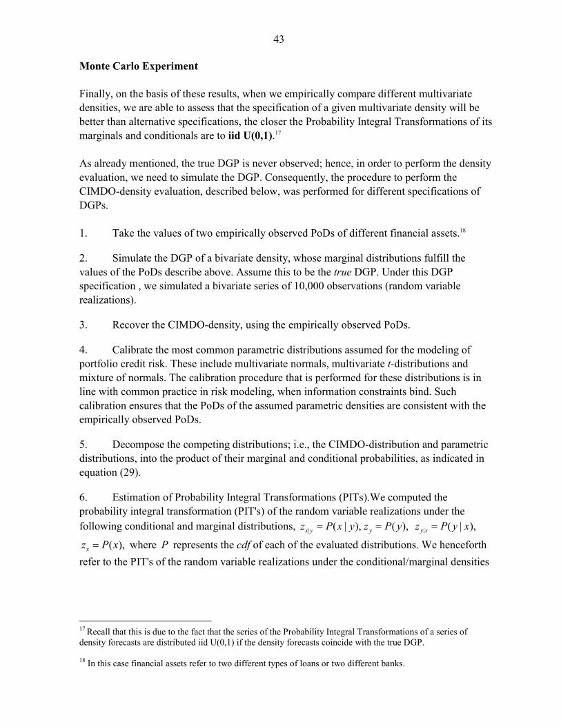
43

Monte Carlo Experiment Finally, on the basis of these results, when we empirically compare different multivariate densities, we are able to assess that the specification of a given multivariate density will be better than alternative specifications, the closer the Probability Integral Transformations of its marginals and conditionals are to iid U(0,1).17 As already mentioned, the true DGP is never observed; hence, in order to perform the density evaluation, we need to simulate the DGP. Consequently, the procedure to perform the CIMDO-density evaluation, described below, was performed for different specifications of DGPs. 1. Take the values of two empirically observed PoDs of different financial assets.18

2. Simulate the DGP of a bivariate density, whose marginal distributions fulfill the values of the PoDs describe above. Assume this to be the true DGP. Under this DGP specification , we simulated a bivariate series of 10,000 observations (random variable realizations).

3. Recover the CIMDO-density, using the empirically observed PoDs.

4. Calibrate the most common parametric distributions assumed for the modeling of portfolio credit risk. These include multivariate normals, multivariate t-distributions and mixture of normals. The calibration procedure that is performed for these distributions is in line with common practice in risk modeling, when information constraints bind. Such calibration ensures that the PoDs of the assumed parametric densities are consistent with the empirically observed PoDs.

5. Decompose the competing distributions; i.e., the CIMDO-distribution and parametric distributions, into the product of their marginal and conditional probabilities, as indicated in equation (29).

6. Estimation of Probability Integral Transformations (PITs).We computed the probability integral transformation (PIT's) of the random variable realizations under the following conditional and marginal distributions, | ( | ), ( ), x y yz P x y z P y= = | ( | ),y xz P y x=

( ),xz P x= where P represents the cdf of each of the evaluated distributions. We henceforth refer to the PIT's of the random variable realizations under the conditional/marginal densities

17 Recall that this is due to the fact that the series of the Probability Integral Transformations of a series of density forecasts are distributed iid U(0,1) if the density forecasts coincide with the true DGP. 18 In this case financial assets refer to two different types of loans or two different banks.

44

as z-variables. We obtained the z-variables for each of the distributional specifications that we evaluated and compared.19

7. Testing for iid ( , )U 0 1 . Our aim was to assess whether a bivariate density specification is correct by testing whether the series /x yz , yz , /y xz , xz were iid. ( , )U 0 1 . Testing for iid ( , )U 0 1 is usually done in two stages. First the iid assumption is tested and then, conditional on the series being iid, the uniform distribution is tested.

(i) Test for the iid assumption. As we proved above, the PIT's of the marginal and conditional densities in which a multivariate distribution can be decomposed, are independent at a given period of time; therefore, there is no need to test for independence.20 (ii) Test for the uniform distribution assumption. Conditional on the series being independent, we proceeded to test for the uniform distribution assumption.

Note that if ( ) ( , )F z ∼ U 0 1 and [ ]0,1z∈ , then ( )F z z= for [ ]0,1 .z∈ Thus the cdf of z is a

45o degree line. Equivalently, the cdf of the PIT's of the random variable realizations under the true DGP will be a 45o degree line if they are uniform distributed. Thus, in order to assess the correctness of a given density specification, we plotted the empirical cdf's of their z-variables and checked how closely these were to the 45o degree line.21 Results Given the highly restrictive data sets that is available (only PoDs, representing partial information of the marginal densities) for the proper specification of all the competing distributions, we never expected to obtain a series of PIT’s that would be iid U(0,1). We rather focused on the relative improvements of one specification versus another by analyzing how close their series of probability integral transformations are to iid U(0,1). Results show that under this criterion, CIMDO-distributions outperform parametric distributions along the whole domain of the distribution; however, it is in the region of default

19 These distributions were the standard normal, the conditional normal, the conditional t-distribution, the mixture model and CIMDO. We henceforth refer to the PIT's obtained under each of these parametric distributions as: NStd, NCon, TCon, NMix and CIMDO respectively. 20 In time series frameworks, auto-correlation coefficients (ACF's) and Ljung-Box-Q-statistics of the z-variables are used to test for independence. At a given period of time, the z-variables are independent, as it was proved above. Therefore, it is not necessary to test for independence. 21 We also computed the Kolmogorov-Smirnov (K-S) tests with 0H : ( , )F = U 0 1 , aH : ( , )F ≠ U 0 1 . K-S tests results are presented in Segoviano (2006b).

45

of the CIMDO-derived distribution (upper right corner) that the improvement is best. This result is consistent with the fact that the information embedded in the CIMDO-derived density, via the moment-consistency constraints, is information of the region of default. Achievement of better accuracy in the upper right corner of the empirical cdf is important. This is because this is the range of the distribution’s domain that has greatest relevance in estimating extreme losses of a portfolio of financial assets.. This is because it represents, for each of the assets making up the portfolio, the probability of going into default. Hence the possibility to model probability densities that improve estimation in this particular region is of relevance. As an example of the results of the Monte Carlo experiment, we reproduce the following figures.

Density Evaluation

0 0.1 0.2 0.3 0.4 0.5 0.6 0.7 0.8 0.9 10

0.1

0.2

0.3

0.4

0.5

0.6

0.7

0.8

0.9

1

Zx/y

F(Zx

/y)

Empirical CDF Zx/y

TconCIMDONStdTrue DGP

0 0.1 0.2 0.3 0.4 0.5 0.6 0.7 0.8 0.9 10

0.1

0.2

0.3

0.4

0.5

0.6

0.7

0.8

0.9

1

Zy

F(Zy

)

Empirical CDF Zy

TConCIMDONStdTrue DGP


In these figures, we compare the empirical cdf’s of the |x yz and yz variables respectively,

corresponding to CIMDO, NStd, TCon and the true-DGP ( 45o degree line). It is clear that CIMDO’s

46

distribution outperforms NStd and TCon along the whole integration domain of the distribution. However, it is in the region of default (upper right corner) where improvements are the best. CIMDO: Copula Evaluation As described in Box 1, copula functions are multivariate distributions; however, with the particularity that their marginal distributions are uniform on the interval [0,1]. Hence, they can be evaluated as any other multivariate density. Nonetheless, as described in equation (20), the first step in the evaluation procedure is to decompose a multivariate density into the product of its marginal and conditional densities. Consequently, it necessary to show that a copula function can be decomposed into the product of its marginal and conditional distributions. Once such decomposition is performed, the marginal and conditionals can be evaluated under the PIT criterion, following exactly the same procedure than the one

described above. A copula function was defined as, [ ]( ) ( ) ( ) ( )

( ) ( ) ( ) ( )

1 1

1 1

,, .

g F u H vc u v

f F u h H v

− −

− −

⎡ ⎤⎣ ⎦=

⎡ ⎤ ⎡ ⎤⎣ ⎦ ⎣ ⎦

This represents the bivariate density function of the variables U and V. This density function can be decomposed into ( , ) ( ) ( | ),c u v c v c u v= ⋅ and ( , ) ( ) ( | ).c u v c u c v u= ⋅ In the interest of parsimony, we focus on the first case. The conditional density function of U given some v is

| ( | ) ( , )u vc u v c u v= because the marginal density function of V is the constant 1. Therefore,

| |0( | ) ( | )

u

u v u vC u v c u v du= ∫ , from the copula definition, this is equivalent

to,( ) ( ) ( ) ( )

( ) ( ) ( ) ( )

1 1

| 1 10

,( | )

u

u v

g F u H vC u v du

f F u h H v

− −

− −

⎡ ⎤⎣ ⎦=

⎡ ⎤⎡ ⎤⎣ ⎦ ⎣ ⎦

∫ . Since 1( ) ( ),U F x x F u−= ⇔ = we get

1( )x F u−= , thus, ( ) ( )

[ ] ( ) ( )( )

1

| 1

,( | ) ,

x

u v

g x H vC u v dF x

f x h H v

−

−−∞

⎡ ⎤⎣ ⎦=

⎡ ⎤⎣ ⎦

∫

( ) ( )[ ] ( ) ( )

( )1

| 1

,( | ) ,

x

u v

g x H vC u v f x dx

f x h H v

−

−−∞

⎡ ⎤⎣ ⎦=

⎡ ⎤⎣ ⎦

∫

( ) ( )( ) ( )

1

| 1

,( | ) ,

x

u v

g x H vC u v dx

h H v

−

−−∞

⎡ ⎤⎣ ⎦=⎡ ⎤⎣ ⎦

∫

( ) ( )1

| |

,( | ) ( | )

x

u v x y

g x H yC u v dx G x y

h y

−

−∞

⎡ ⎤⎣ ⎦= =

⎡ ⎤⎣ ⎦∫ ( 22)

Thus, the distribution of U given some fixed v is uniform. Recall the PIT proof. Once this decomposition is performed, the marginal and conditional copulas can be evaluated under the PIT criterion. In order to do this, we have carried out a Monte Carlo experiment similar to the one described above.

47

APPENDIX IV. ESTIMATION OF PROBABILITIES OF DISTRESS OF INDIVIDUAL BANKS The various procedures to obtain individual banks’ PoDs that we have analyzed include the structural approach (SA), Credit Default Swaps (CDS) spreads and out-of-the-money (OOM) option prices. Here we present a summary of the advantages and disadvantages of each of these procedures. The Structural Approach The structural approach is widely utilized to model PoDs.22 The basic premise of the SA assumes that a firm’s underlying asset value evolves stochastically over time, triggering default when it falls below a pre-specified barrier, henceforth, called the default-threshold, which is modeled as a function of the firm's leverage structure. Thus, the PoD of a firm is determined by: (a) the market value of its assets, AV ; (b) the uncertainty or volatility of the asset value, Aσ ; and (c) the degree of leverage or the extent of the firm’s contractual liabilities, measured as the book value of liabilities at time t, tD (with maturity T ). Under the most basic and popular version of the SA, the market value of firms’ assets, AV and volatilities, Aσ are modeled following the Merton (1974) framework, using information concerning equity prices. Hence, bank equity prices and the balance sheets of each of the banks under analysis constitute the main variables that are necessary to estimate marginal PoDs under the SA. These variables are usually available for the largest banks of a wide range of countries, both developed and developing. Such information availability is an important advantage of this approach. Moreover, this approach allows an explicit definition of default. It summarizes in the PoD—its measure of default—the market perceptions (via equity prices) and financial conditions (via the default threshold) of a firm. This explicit definition of default is economically intuitive and allows a separate analysis of the factors determining default, thereby improving our understanding of default. The SA is thereby better than studies that analyze changes (decreases) in asset returns without explicitly defining default. The latter bring ambiguity to the definition of default since they do not explicitly have a threshold beyond which changes in asset returns would cause a firm to default. Unfortunately, the SA—as any other approach—poses challenges for its correct empirical implementation. The proper specification and calibration of the distribution that firms’ asset values are assumed to follow is a difficult task, even if information on stock prices is available, since the latter is only a proxy for asset values.23 Moreover, empirically, it has been observed that financial firms’ logarithmic asset values do not follow normal 22 The CreditMetrics methodology (Gupton, Finger, and Bhatia, 1997) and Moody’s-KMV methodology (Crosbie, 1998) are applications built upon this approach. 23 Wile common practice in the industry is to use equity return volatilities and correlations as proxies for asset return volatilities and correlations, Servigny and Renault (2002) and Schonbucher (2003) document the fact that equity return second moments tend to be significantly higher than asset return ones.

48

distributions. So, different parametric distributions have been proposed to improve the modeling of the stochastic behavior of the asset values in the structural approach. However, for any of these parametric assumptions, the availability of variables, or proxies, indicating the evolution of the firms’ underlying asset values is of crucial importance for both their proper calibration and implementation. Additionally, PoDs are very sensitive to volatility values. There are numerous ways to estimate realized and implied volatilities, which may be appropriate under different circumstances, and that may produce significantly different volatility values. To obtain a correct estimation of volatility can become demanding. In our view, the sensitivity of PoDs to volatility values implies that PoDs appear to be too sensitive to factors that affect the aggregate level and variance of the equity market rather than the particular robustness (or fragility) of the banking system. CDS Spreads The estimation of PoDs from CDS spreads is not subject to the modeling of the distribution of asset prices or the explicit estimation of CDS volatilities (see Box 2). These characteristics might represent an advantage over the SA. Nevertheless, even if the explicit estimation of asset distributions and volatility is avoided under the CDS approach, PoDs inferred from CDS spreads are affected by liquidity in the particular CDS market, and generalized risk aversion in the financial system. Out-of-the-Money Option Prices Under the fundamental theorem of asset pricing,24 the estimation of PoDs from out-of-the-money (OOM) calls or puts is not subject to the explicit estimation of the distribution of asset prices, volatilities, recovery rates (RR), price of delivery options, or convenience. Moreover—for some banking sectors—liquid markets of plain vanilla options might be more extensive than liquid markets of CDS; hence, it might be possible to implement this approach to estimate the PoDs of a larger set of banks in developed and developing economies. Nonetheless, it has to be considered that CDS markets are growing and becoming liquid very rapidly; thus, in some cases, the liquidity of plain vanilla option markets might soon be overtaken by the liquidity of CDS markets. However, this methodology to estimate PoDs is subject to (i) the availability of information of OOM option prices at different strike prices, and (ii) model calibrations, that in some cases might become cumbersome. Given the advantages and disadvantages of each of the described methodologies, we are currently performing a research project to investigate empirically what is the most appropriate methodology to estimate individual banks’ PoDs. Note, however that PoDs are exogenous variables to the estimation of the banking system multivariate density; hence, the CIMDO methodology can be implemented with PoDs derived by any method that is considered the most appropriate or that is available in different countries.

24 For an excellent presentation, we refer readers to Neftci ( 2004).

49

References

Altman, E., A. Elizondo, and Miguel Segoviano, 2002, “Medicion Integral del Riesgo de

Credito,” edited Limusa, Mexico.

Athanosopoulou, M., Miguel Segoviano, and Alexander Tieman, 2009, “Banks’ Probability of Default: Which Methodology, When, and Why?” IMF Working Paper (forthcoming) (Washington: International Monetary Fund).

Aspachs, O., and others, 2006, “Searching for a Metric for Financial Stability,” London School of Economics, Financial Markets Group, Special Paper No. 167.

Basel Committee on Banking Supervision, 1988, “International Convergence of Capital

Measurement and Capital Standards,” Basel, July 1988. Berger, A., and G. Udell, 1990, “Collateral, Loan Quality, and Bank Risk,” Journal of

Monetary Economics, Vol. 25, pp. 21–42. ———, 2003, “The Institutional Memory Hypothesis and the Procyclicality of Bank

Lending Behavior,” Bank for International Settlements Working Paper No. 125. Black, F., and M. Scholes, 1973, “The Pricing of Options and Corporate Liabilities,” Journal

of Political Economy, Vol. 81, pp. 637–59. Bank for International Settlements, 1999, “The Monetary and Regulatory Implications of

Changes in the Banking Industry,” Bank for International Settlements Conference Papers No.7.

———, 2001, 71st Annual Report. Borio, C., and W. Fritz, 1995, “The Response of Short-Term Bank Lending Rates to Policy

Rates: A Cross-Country Perspective,” Bank for International Settlements Working Paper No. 27.

Bordo, M., and others, 2001, “Financial Crises: Lessons from the Last 120 Years,” Economic Policy.

Butler, J., and B. Schachter, 1998, “Estimating Value-at-Risk with a Precision Measure by

Combining Kernel Estimation with Historical Simulation,” Review of Derivatives Research Vol. 1, pp. 371–90.

Caprio, G., and D. Klingebiel, 1996, “Bank Insolvency: Cross-Country Experiences,”

(Washington: World Bank). Crosbie, P., and J. Bohn, 1999, “Modeling Default Risk,” KMV LLC.

50

Danielsson, J. and C. G. de Vries, 1997, “Tail Index and Quantile Estimation with Very High

Frequency Data,” JEF, Vol. 4, pp. 241–57. De Bandt, O., and P. Hartmann, 2001, “Systemic Risk: A Survey” in C. Goodhart, and G.

Illing, eds., Financail Crisis, Contagion and the Lender of Last Resort: A Book of Readings, pp 249-298 (Oxford: Oxford University Press).

De Vries, C., 2005, “The Simple Economics of Bank Fragility,” Journal of Banking and Finance No. 29, pp 803-25. Demirgüc-Kunt, A., and E. Detriagiache, 1998, “The Determinants of Banking Crises:

Evidence from Developing and Developed Countries,” Staff Papers, International Monetary Fund, Vol. 45, No. 1.

———, 1999, “Financial Liberalization and Financial Fragility,” edited by B. Pleskovic and

J. Stiglitz in Proceedings of the World Bank Annual Conference on Development Economics.

———, 2005, “Cross-Country Empirical Evidence of Systemic Banking Distress: A

Survey,” IMF Working Paper 05/96 (Washington: International Monetary Fund). Diebold, F., T. Gunther, and A. Tay, 1998, “Evaluating Density Forecasts with Applications

to Financial Risk Management,” IER, Vol. 39, pp. 863–83. Diebold, F., J. Hahn, and A. Tay, 1999, “Multivariate Density Forecast Evaluation and

Calibration in Financial Risk Management: High-Frequency Returns on Foreign Exchange,” The Review of Economics and Statistics, Vol. 81(4), pp. 661–73.

Dooley, M., 1997, “A Model of Crises in Emerging Markets,” NBER, Working Paper No. 6300. Duffie, J. D., and K. J. Singleton, 1999, “Modelling Term Structures of Defaultable Bonds,”

Review of Financial Studies Vol. 12, pp. 687–720. Eichengreen, B., and C. Areta, 2000, “Banking Crises in Emerging Markets: Presumptions

and Evidence,” Center for International and Development Economics Research Paper, C00-115.

Eichengreen, B., and M. Bordo, 2003, “Crises Now and Then: What Lessons From the Last

Era of Financial Globalization,” Edited by P. Mizen, Chapter 3 in Monetary History, Exchange Rates, and Financial Markets; Essays in honor of Charles Goodhart, Vol. 2, pp. 52–91 (Cheltenham: Edward Elgar).

Embrechs, P., A. McNeil, and D. Straumann, 1999, “Correlation and Dependence Properties in Risk Management: Properties and Pitfalls,” Working Paper, RiskLab, ETH, Zurich.

51

Flood, R., and N. Marion, 1999, “Perspectives on the Recent Currency Crisis Literature,”

International Journal of Finance and Economics, Vol. 4, 1, pp. 1–26. Frey, R., and A.J. McNeil, 2001, ”Modelling Dependent Defaults,”. Working Paper, Department of Mathematics, ETH Zurich. Glasserman, P., P. Heidelberger, and P. Shahabuddin, 2000, “Portfolio Value-at-Risk with

Heavy-Tailed Risk Factors,” Money, Economics, and Finance Working Paper (Columbia: Columbia Business School, Columbia University.).

Goldstein, M., G. Kaminsky, and C. Reinhart, 2000, “Assessing Financial Vulnerability: An

Early Warning System for Emerging Markets,” Institute for International Economics, Washington DC.

Goodhart, Charles, 1995, “Price Stability and Financial Fragility,” edited by K. Sawamoto,

Z. Nakajima, and H. Taguchi in Financial Stability in a Changing Environment, St. Martin’s Press.

Goodhart, Charles, and Boris Hofmann, 2003, “Deflation, Credit, and Asset Prices,” forthcoming in P. Siklos and R. Burdekin, The Anatomy of Deflation, Cambridge University Press. Goodhart, Charles, Boris Hofmann, and Miguel Segoviano, 2004, “Bank Regulation and

Macroeconomic Fluctuations,” Oxford Review of Economic Policy, Vol. 20, No. 4, pp. 591–615.

Goodhart, Charles, and Miguel Segoviano, 2004, “Basel and Procyclicality: A Comparison

of the Standardized and IRB Approaches to an Improved Credit Risk Method,” London School of Economics, Financial Markets Group, Discussion Paper 524.

Goodhart, Charles, Boris Hofmann, and Miguel Segoviano, 2006, “Default, Credit Growth, and Asset Prices” IMF Working Paper 06/223 (Washington: International Monetary Fund). Goodhart, Charles, P. Sunirand, and D. Tsomocos, 2006, “A Model to Analyse Financial Fragility”, Economic Theory , Vol. 27 (1), pp. 107-42. Gupton, M., C. Finger, and M. Bhatia, 1997, “Credit Metrics Technical Document,” Morgan Guaranty Trust Company, Risk Management Research. Hartmann, P., S. Straetmans, and C. De Vries, 2001, “Asset Market Linkages in Crisis Periods,” European Central Bank, Working Paper Series, No. 71. Hodrick, R., and E. Prescott, 1980, “Post-War U.S. Business Cycles: An Empirical

52

Investigation,” Discussion Paper No. 451, Carnegie-Mellon University. Heiskanen, R., 1993, “The Banking Crisis in the Nordic Countries,” Kansallis Economic Review, Vol. 2, pp. 13–19. Hoelscher, D., 2006, “Bank Restructuring and Resolution,” International Monetary Fund:

Monetary and Financial Systems Dept. October 1, 2006. Hofmann, B., 2001, “The Determinants of Private Sector Credit in Industrialized Countries: Do Property Prices Matter?” BIS Working Paper No. 108. Hoskin, J.R.M., G. Bonti, and D. Siegel, 2000, “Beyond the Lognormal,” Risk 13, No. 5 (May), pp. 59–62. Huang, X., 1992, “Statistics of Bivariate Extreme Values,” Tinbergen Institute Research Series, Ph.D. Thesis, No 22, Erasmus University, Rotterdam, Netherlands. Jaynes, E., 1957, “Information Theory and Statistical Mechanics,” Physics Review Vol. 106, pp. 620–30. Jaynes, E., 1984, “Prior Information and Ambiguity in Inverse Problems,” Edited by D.W.

McLaughlin in Inverse Problems, pp.151–66, SIAM Proceedings, American Mathematical Society, Providence, Rhode Island.

Judge, G., and A. Golan, 1992, “Recovering Information in the Case of Ill-Posed Inverse

Problems with Noise,” University of California Berkeley. Kaminsky, G., S. Lizondo, and C. Reinhart, 1998, “Leading Indicators of Currency Crises,”

Staff Papers, International Monetary Fund, Vol. 5 (January), pp. 1–48. ———, and C. Reinhart, 1996, “Banking and Balance of Payments Crises: Models and

Evidence,” Board of Governors of the Federal Reserve Working Paper (Washington: Board of Governor of the Federal Reserve).

———, and C. Reinhart, 1999, “The Twin Crisis: The Causes of Banking and Balance

of Payments Problems,” American Economic Review, Vol. 89, pp. 473–500. ———, and S. Schmukler, 2003, “Short-Run Pain, Long-Run Gain: The Effects of

Financial Liberalization,” NBER Working Paper 9787. Kiyotaki, N., and J. Moore, 1997, “Credit Cycles,” Journal of Political Economy, Vol. 105,

pp. 211–48.

53

Krugman, P., 1979, “A Model of Balance of Payments Crises,” Journal of Money, Credit, and Banking, Vol. II(3), pp. 311–25.

Knight, M., and J. Santaella, 1997, “Economic Determinants of IMF\ Financial

Arrangements,” Journal of Development Economics, Vol. 54, pp. 405–36. Kullback, S., and R. Leibler, 1951, “On Information and Sufficiency,” Annals of

Mathematical Statistics, Vol. 22, 79–86. Kullback, J., 1959, “Information Theory and Statistics”, (New York: John Wiley). McLachlan, G., and K. Basford, 1987, “Mixture Models: Inference and Applications to

Clustering, Marcel Dekker,” New York and Basel. McKinnon, R., and H. Pill, 1996, “Credible Liberalizations and International Capital Flows:

The Over Borrowing Syndrome,” edited by T. Ito and Krueger in Financial Deregulation and Integration in East Asia, pp. 7–45 (Chicago: University of Chicago Press).

Merton, R., 1974, “On the Pricing of Corporate Debt: The Risk Structure of Interest Rates,”

The Journal of Finance, Vol. 29, pp. 449–70.

Mina, J., and Y. Xiao, 2001, “Return to RiskMetrics: The Evolution of a Standard,” RiskMetrics.

Minsky, H., 1982, “Can It Happen Again?” Essays on Instability and Finance, M.E. Sharpe. Mishkin, F., 1997, “Understanding Financial Crises: A Developing Country Perspective,”

edited by Michael Bruno and Boris Pleskovic in Annual World Bank Conference on Development Economics 1996, Washington, DC, International Bank for Reconstruction and Development, pp. 29–61.

Nelsen, R. (1999), "An Introduction to Copulas", Lecture Notes in Statistics 139, Springer.

Obstfeld, M., 1995, “Models of Currency Crises with Self-Fulfilling Features,” NBER Working Paper 5285 (Cambridge, Massachusetts: MIT Press).

Obstfeld, M., and K. Rogoff, 1995, “The Mirage of Fixed Exchange Rates,” NBER Working

Paper 5191 (Cambridge, Massachusetts: MIT Press). OECD, 2006, “2006 Economic Review, Denmark,” Economic and Development Review

Committee, (Paris). Pukelsheim, F., 1994, “The Three Sigma Rule,” American Statistician, Vol. 48(4), pp. 88–91. Reinhart, C., and I. Tokatlidis, 2001, “Before and After Financial Liberalization,” University

54

of Maryland, mimeo. Segoviano, Miguel, 1998, “An Structural Approach for Portfolio Credit Risk vs.

Creditmetrics” London School of Economics, mimeo. Segoviano, Miguel, and P. Lowe, 2002, “Internal Ratings, the Business Cycle and Capital

Requirements: Some Evidence from an Emerging Market Economy,” BIS Working Paper 117, LSE/FMG discussion paper 428.

Segoviano, Miguel, 2004, “A System for Measuring Credit Risk When Only Limited Data is Available,” Credit Risk International, London, October 2004. ———, 2006a, “The Conditional Probability of Default Methodology,” Financial Markets

Group, London School of Economics, Discussion Paper 558. ———, 2006b, “The Consistent Information Multivariate Density Optimizing

Methodology,” Financial Markets Group, London School of Economics, Discussion Paper 557.

Segoviano, Miguel, and P. Padilla, 2006, “Portfolio Credit risk and Macroeconomic Shocks:

Applications to Stress Testing under Data Restricted Environments,” Working Paper WP/06/283 (Washington: International Monetary Fund).

Shannon, C., 1948, “A Mathematical Theory of Communication,” Bell System, Technical

Journal, Vol. 27, pp. 379–423. Vassalou, M., and Y. Xing, 2002, “Default Risk in Equity Returns,” Columbia University

Working Paper. Zangari, P., 1996, “An Improved Methodology for Measuring VaR,” RiskMetrics Monitor,

2nd Quarter, pp.7–25.

miguel a. segoviano and charles goodhart - imf · banking stability measures prepared by miguel a....

Documents