microstructure of systems with competition
TRANSCRIPT

Washington University in St. LouisWashington University Open Scholarship
All Theses and Dissertations (ETDs)
7-25-2012
Microstructure of Systems with CompetitionSaurish ChakrabartyWashington University in St. Louis
Follow this and additional works at: https://openscholarship.wustl.edu/etd
This Dissertation is brought to you for free and open access by Washington University Open Scholarship. It has been accepted for inclusion in AllTheses and Dissertations (ETDs) by an authorized administrator of Washington University Open Scholarship. For more information, please [email protected].
Recommended CitationChakrabarty, Saurish, "Microstructure of Systems with Competition" (2012). All Theses and Dissertations (ETDs). 945.https://openscholarship.wustl.edu/etd/945

WASHINGTON UNIVERSITY IN ST. LOUIS
Department of Physics
Dissertation Examination Committee:Zohar Nussinov, ChairKenneth F. KeltonRonald Lovett
Michael C. OgilvieAlexander SeidelJung-Tsung Shen
Microstructure of Systems with Competition
by
Saurish Chakrabarty
A dissertation presented to theGraduate School of Arts and Sciences
of Washington University inpartial fulfillment of the
requirements for the degreeof Doctor of Philosophy
August 2012
Saint Louis, Missouri

ABSTRACT OF THE DISSERTATION
Microstructure of Systems with Competition
by
Saurish Chakrabarty
Doctor of Philosophy in Physics
Washington University in St. Louis, 2012
Professor Zohar Nussinov, Chairperson
The micro-structure of systems with competition often exhibits many universal fea-
tures. In this thesis, we study certain aspects of these structural features as well as
the microscopic interactions using disparate exact and approximate techniques. This
thesis can be broadly divided into two parts.
In the first part, we use statistical mechanics arguments to make general state-
ments about length and timescales in systems with two-point interactions. We demon-
strate that at high temperatures, the correlation function of general O(n) systems
exhibits a universal form. This form enables the extraction of microscopic interaction
potentials from the high temperature correlation functions. In systems with long
range interactions, we find that the largest correlation length diverges in the limit of
high temperatures. We derive an exact form for the correlation function in large-n
systems with general two-point interactions at finite temperatures. From this, we
obtain some features of the correlation and modulation lengths in general systems in
the large-n limit. We derive a new exponent characterizing modulation lengths (or
times) in systems in which the modulation length (or time) either diverges or becomes
ii

constant as a parameter, such as temperature exceeds a threshold value.
In the second part of this thesis, we study the micro-structure of a metallic glass
system using molecular dynamics simulations. We use both classical and first prin-
ciples simulation to obtain atomic configurations in the liquid as well as the glassy
phase. We analyze these using standard methods of local structure analysis – calcu-
lation of pair correlation function and structure factor, Voronoi construction, calcu-
lation of bond orientational order parameters and calculation of Honeycutt indices.
We show the enhancement of icosahedral order in the glassy phase. Apart from this,
we also use the techniques of community detection to obtain the inherent structures
in the system using an algorithm which allows us to look at arbitrary length-scales.
iii

Acknowledgements
First of all, I would like to thank my father Tapan Kumar Chakrabarty, my mother
Dipa Chakrabarty and my sister Patrali Chakrabarty for providing great support and
encouragement. I also thank Dida, Jethu, Mama, Mani and Mamoni.
My roommates Manojit and Poulomi made living in St Louis a lot of fun along with
Shatadal, Tanika, Satyaki, Mrinmoyda, Maitrayee, Somendra, Satya, Pinaki, Nidhi,
Debajit, Sudeshna and Kumar and my classmates Adam Hajari, Ben Burch, Narelle,
David Shane, Hiromichi, Seth, Dimitris, Dihui, Wei, Amber and Jason. I thank the
physics mentors of 2006-07 for frequently taking us out for free food. Special thanks
to the “Mesh” members – Subhadip, Zoheb and Mainak Mukherjee. Many thanks to
Rudresh, Santi, Mainak Das, Shradha, Aditi, Krishanu, Sanhita, Mithun and Girish.
I thank my past teachers S. K. Bhattacharyya and Ananda Dasgupta for inspiring
me to pursue a career in physics.
Thanks to all my committee members – Ken Kelton, Ronald Lovett, Mike Ogilvie,
Alex Seidel and JT Shen.
I thank Mike Widom and Marek Mihalkovic for teaching me numerous computa-
tional methods. I also thank Mike for his hospitality during my stay at Pittsburgh.
iv

Acknowledgements
I thank my group members – Peter, Dandan and Patrick, my former group mem-
bers Matt, Adam Eggebrecht, Sebastian, Jing, Shouting and Blake, and my former
adviser Ralf Wessel.
Special thanks to Julia and Sarah. Sai has taught me a lot of Linux tricks and I
thank him greatly for that.
My office was a great place to work in. For that I thank Seth, Mark, Hiromichi,
Zhenyu, Julia, Shouting, Dan, Hossein and Sophia.
Lastly, I thank my adviser Zohar Nussinov for being a great inspiration. With his
great versatility, he can come up with a new research idea every time a student meets
him.
v

To my father, mother and sister.
vi

Contents
Abstract ii
Acknowledgements iv
List of Figures xi
List of Tables xviii
1 Introduction 11.1 Correlation functions . . . . . . . . . . . . . . . . . . . . . . . . . . . 21.2 Structural features and universality . . . . . . . . . . . . . . . . . . . 31.3 Structure of liquids and glasses . . . . . . . . . . . . . . . . . . . . . 51.4 Outline . . . . . . . . . . . . . . . . . . . . . . . . . . . . . . . . . . . 7
2 Systems of study 92.1 Introduction . . . . . . . . . . . . . . . . . . . . . . . . . . . . . . . . 92.2 Systems of study . . . . . . . . . . . . . . . . . . . . . . . . . . . . . 92.3 O(n) systems and the large-n limit . . . . . . . . . . . . . . . . . . . 112.4 Obtaining correlation and modulation lengths from the momentum
space correlation function . . . . . . . . . . . . . . . . . . . . . . . . 13
3 High temperature correlation functions 153.1 Introduction . . . . . . . . . . . . . . . . . . . . . . . . . . . . . . . . 153.2 The universal form of the high temperature correlation functions . . . 173.3 High temperature correlation lengths . . . . . . . . . . . . . . . . . . 23
3.3.1 Decaying lengthscales . . . . . . . . . . . . . . . . . . . . . . . 233.3.2 Diverging lengthscales . . . . . . . . . . . . . . . . . . . . . . 24
3.4 Generalized Debye length (and time) scales . . . . . . . . . . . . . . . 273.5 Generalizations . . . . . . . . . . . . . . . . . . . . . . . . . . . . . . 30
3.5.1 Disorder . . . . . . . . . . . . . . . . . . . . . . . . . . . . . . 303.5.2 Fluids . . . . . . . . . . . . . . . . . . . . . . . . . . . . . . . 313.5.3 General multi-component interactions . . . . . . . . . . . . . . 313.5.4 Bose/Fermi gases . . . . . . . . . . . . . . . . . . . . . . . . . 32
3.6 Approximate Methods . . . . . . . . . . . . . . . . . . . . . . . . . . 353.6.1 Ginzburg-Landau φ4-type theories . . . . . . . . . . . . . . . . 35
vii

Contents
3.6.2 Correlation functions in the large-n limit . . . . . . . . . . . . 363.6.3 Ornstein-Zernike equation . . . . . . . . . . . . . . . . . . . . 38
3.7 Conclusions . . . . . . . . . . . . . . . . . . . . . . . . . . . . . . . . 39
4 Competing interactions 404.1 Ground-state stripe width for Ising systems: lattice versus continuum
theory scaling . . . . . . . . . . . . . . . . . . . . . . . . . . . . . . . 484.2 Correlation Functions in the large-n limit: general considerations . . . 504.3 Large-n Results . . . . . . . . . . . . . . . . . . . . . . . . . . . . . . 55
4.3.1 The low temperature limit: a criterion for determining an in-crease or decrease of the modulation length at low temperatures 55
4.3.2 A correspondence between the temperature T ∗ at which themodulation length diverges and the critical temperature Tc . . 59
4.3.3 Crossover temperatures: emergent modulations . . . . . . . . 604.3.4 First order transitions in the modulation length . . . . . . . . 68
4.4 Example systems . . . . . . . . . . . . . . . . . . . . . . . . . . . . . 694.4.1 Numerical evaluation of the Correlation function . . . . . . . . 704.4.2 Coexisting short range and screened Coulomb interactions . . 714.4.3 Full direction and location dependent dipole-dipole interactions 804.4.4 Dzyaloshinsky- Moriya Interactions . . . . . . . . . . . . . . . 81
4.5 Conclusions . . . . . . . . . . . . . . . . . . . . . . . . . . . . . . . . 82
5 Universality of modulation length (and time) exponents 845.1 Introduction . . . . . . . . . . . . . . . . . . . . . . . . . . . . . . . . 845.2 A universal domain length exponent – Details of analysis . . . . . . . 86
5.2.1 Crossovers at general points in the complex k-plane . . . . . . 875.2.2 Branch points . . . . . . . . . . . . . . . . . . . . . . . . . . . 935.2.3 A corollary: Discontinuity in modulation lengths implies a ther-
modynamic phase transition . . . . . . . . . . . . . . . . . . . 965.2.4 Diverging correlation length at a spinodal transition . . . . . . 975.2.5 Conservation of characteristic length scales . . . . . . . . . . . 98
5.3 O(n) systems . . . . . . . . . . . . . . . . . . . . . . . . . . . . . . . 995.3.1 Low temperature configurations . . . . . . . . . . . . . . . . . 995.3.2 High temperatures . . . . . . . . . . . . . . . . . . . . . . . . 1005.3.3 Large-n Coulomb frustrated ferromagnet – modulation length
exponent at the crossover temperature T∗ . . . . . . . . . . . . 1015.3.4 An example with νL 6= 1/2 . . . . . . . . . . . . . . . . . . . . 1025.3.5 An example in which T∗ is a high temperature . . . . . . . . . 103
5.4 Crossovers in the ANNNI model . . . . . . . . . . . . . . . . . . . . . 1045.5 Parameter extensions and generalizations . . . . . . . . . . . . . . . . 1075.6 Implications for the time domain: Josephson time scales . . . . . . . 111
viii
Contents
5.7 Chaos and glassiness . . . . . . . . . . . . . . . . . . . . . . . . . . . 1125.8 Conclusions . . . . . . . . . . . . . . . . . . . . . . . . . . . . . . . . 120
6 A molecular dynamics study on the micro-structure of Al88Fe5Y7 1236.1 Introduction . . . . . . . . . . . . . . . . . . . . . . . . . . . . . . . . 1236.2 Results . . . . . . . . . . . . . . . . . . . . . . . . . . . . . . . . . . . 1256.3 Methods . . . . . . . . . . . . . . . . . . . . . . . . . . . . . . . . . . 126
6.3.1 Classical molecular dynamics simulation . . . . . . . . . . . . 1266.3.2 First principles molecular dynamics simulation . . . . . . . . . 1316.3.3 Analysis . . . . . . . . . . . . . . . . . . . . . . . . . . . . . . 132
6.4 Observations and inference . . . . . . . . . . . . . . . . . . . . . . . . 1356.4.1 A look at the Al-Fe-Y phase diagram . . . . . . . . . . . . . . 1376.4.2 Honeycutt-Anderson analysis . . . . . . . . . . . . . . . . . . 1416.4.3 Bond orientation . . . . . . . . . . . . . . . . . . . . . . . . . 1446.4.4 Voronoi analysis . . . . . . . . . . . . . . . . . . . . . . . . . . 145
7 Multiresolution network clustering 1487.1 Introduction . . . . . . . . . . . . . . . . . . . . . . . . . . . . . . . . 148
7.1.1 Partitions of large systems into weakly coupled elements . . . 1507.1.2 Community detection method . . . . . . . . . . . . . . . . . . 1507.1.3 Multiresolution network analysis . . . . . . . . . . . . . . . . . 152
7.2 Systems studied . . . . . . . . . . . . . . . . . . . . . . . . . . . . . . 1537.2.1 Ternary model glass former . . . . . . . . . . . . . . . . . . . 1547.2.2 Lennard-Jones glass . . . . . . . . . . . . . . . . . . . . . . . . 157
7.3 Results . . . . . . . . . . . . . . . . . . . . . . . . . . . . . . . . . . . 1587.3.1 Ternary model glass results . . . . . . . . . . . . . . . . . . . 1607.3.2 Binary Lennard-Jones glass results . . . . . . . . . . . . . . . 166
7.4 Conclusions . . . . . . . . . . . . . . . . . . . . . . . . . . . . . . . . 169
Appendix 170A High temperature series expansion of the correlation function . . . . . 170B Relation between the generalized Debye lengths and divergence of the
high temperature correlation lengths . . . . . . . . . . . . . . . . . . 178C Transfer Matrix in the one-dimensional system with Ising spins . . . . 179D Detailed expressions for δLD for different orders p(≥ 3) at which the
interaction kernel has its first non-vanishing derivative . . . . . . . . 181E µ(T ) for the screened Coulomb ferromagnet . . . . . . . . . . . . . . 181F Proof that µ(T ) is an analytic function of T . . . . . . . . . . . . . . 182G Fermi systems . . . . . . . . . . . . . . . . . . . . . . . . . . . . . . . 183
G.1 Zero temperature length scales – Scaling as a function of thechemical potential µ . . . . . . . . . . . . . . . . . . . . . . . 185
ix

Contents
G.2 Finite temperature length scales – Scaling as a function of tem-perature . . . . . . . . . . . . . . . . . . . . . . . . . . . . . . 197
H Euler-Lagrange equations for scalar spin systems . . . . . . . . . . . . 198
x

List of Figures
1.1 Sub-unit-cell resolution image of the electronic structure of a cupratesuperconductor at the pseudo-gap energy. Inset shows Fourier spaceimage of the same figure. Nematic and smectic phases are highlightedusing the red and blue circles respectively. The nematic phase is char-acterized by commensurate wave-vectors ~Q. The smectic wave-vector,on the other hand takes incommensurate values, ~S which is dependenton the amount of doping, albeit weakly. (From Ref. [1]. Reprintedwith permission from AAAS.) . . . . . . . . . . . . . . . . . . . . . . 4
4.1 Reproduced with permission from Science, Ref.[2]. Reversible “strip-out” instability in magnetic and organic thin films. Period (LD) reduc-tion under the constraint of fixed overall composition and fixed numberof domains leads to elongation of bubbles. Left panel (A) in magneticgarnet films, this is achieved by raising the temperature [labeled in (B)in degrees Celsius] along the symmetry axis, H = 0 (period in bot-tom panel, ∼ 10µm) (see Fig. 5). Right panel (B) In Langmuir filmscomposed of phospholipid dimyristolphosphatidic acid (DMPA) andcholesterol (98:2 molar ratio, pH 11), this is achieved by lowering thetemperature at constant average molecular density [period in bottompanel, ∼ 20µm] . . . . . . . . . . . . . . . . . . . . . . . . . . . . . . 43
4.2 −f(z) = −v(k) = µ plotted against z = k2 for purely real andpurely imaginary k’s (T → 0 and T → ∞ respectively). The nega-tive z regime corresponds to temperatures (Lagrange multiplier, µ’s)for which purely imaginary solutions exist. The maximum of the curvein the positive z regime corresponds to the modulations at T = Tc[µ = µmin], which is the maximum temperature at which pure modu-lations exist. . . . . . . . . . . . . . . . . . . . . . . . . . . . . . . . . 61
4.3 Left: Solid line: −v(k) plotted against k; Dashed line: −v(iκ) plottedagainst κ. Right: −f(z) plotted against z. . . . . . . . . . . . . . . . 62
xi

List of Figures
4.4 Illustration of the limit T ∗ → Tc as Q → 0 with vL(k) = 1/k3. Theplot shows −f(z) = −v(k) vs z = k2, for v(k) = Jk2 + Q/k3 withJ = 1 and Q = {1−Blue, 0.1−Green, 0.01−Yellow, 0.001−Red}. ‘*’represents the value of µ∗ and dot represents µmin. . . . . . . . . . . . 65
4.5 The correlator G(x, y) for a two-dimensional screened Coulomb ferro-magnet of size 100 by 100. J = 1, Q = 0.0004, screening length=100
√2. A: µ = µmin = −0.0874, B: µ = µmin + 0.001, C: µ = µmin +
0.003, D: G(x,y) for y = 0 for A(blue)[LD = 20], B(green)[LD = 24]and C(red)[LD = 26]. . . . . . . . . . . . . . . . . . . . . . . . . . . . 71
4.6 The correlator G(x, y) for a two-dimensional dipolar ferromagnet ofsize 100 by 100. J = 1, Q = 0.15. A: µ = µmin = −1.1459, B:µ = µmin + 4× 10⁻⁵, C: µ = µmin + 1× 10⁻³, D: G(x,y) for y = 0 forA(blue)[LD = 14], B(green)[LD = 15] and C(red)[LD = 16]. . . . . . . 72
4.7 Location of the poles with increasing temperature (left to right) in thecomplex k-plane for the Coulomb frustrated ferromagnet. For temper-atures below Tc, all the poles are real. Above Tc, the poles split inopposite directions of the real axis to give rise to two new complexpoles. For Tc < T < T ∗, we have complex poles. At T ∗, pairs of suchpoles meet on the imaginary axis. Above T ∗, the poles split along theimaginary axis. Thus, above T ∗, the poles are purely imaginary. . . . 76
4.8 Trajectory of the poles in the complex k-plane for Tc < T < T ∗ for thescreened Coulomb ferromagnet. The screening length, λ−1 decreasesfrom left to right. In the first figure λ = 0 and λ > (Q/J)1/4 in thelast figure. . . . . . . . . . . . . . . . . . . . . . . . . . . . . . . . . . 76
4.9 Temperature at which the modulation length diverges for a 100× 100Coulomb frustrated ferromagnet plotted versus the relative strength ofthe Coulomb interaction with respect to the ferromagnetic interaction.[Blue:λ = λ0 = 1/(100
√2); Red:λ = 0.999λ0; Black:λ = 1.001λ0] . . . 77
5.1 Schematic showing the trajectories of the singularities of the correlationfunction near a fixed – variable modulation length crossover. Two polesof the correlation function merge at k = k∗ at T = T∗. On the fixedmodulation length side of the crossover point, Re k = q. . . . . . . . . 87
5.2 Location of the poles of the correlation function of the large-n Coulombfrustrated ferromagnet for J = Q = 1 in the complex k-plane. Thecircle and the Y -axis show the trajectory K(T ) of the poles as thetemperature T is varied. . . . . . . . . . . . . . . . . . . . . . . . . . 91
5.3 Location of the poles of the correlation function of the system in Eq.(5.31) for large ls (small screening) in the complex k-plane. . . . . . . 103
5.4 The coupling constants in the three-dimensional ANNNI model. . . . 105
xii

List of Figures
5.5 Existence of incommensurate phases between the commensurate re-gions in the phase diagram of the ANNNI model. (a) Mean fieldphase diagram of the ANNNI model in three dimensions. The shadedregions show higher order commensurate phases which have variablemodulation length incommensurate phases in between (From Ref. [3].Reprinted with permission from APS.) (b) Phase diagram for thethree-dimensional ANNNI model using a modified tensor product vari-ational approach (From Ref. [4]. Reprinted with permission fromAPS.) (c) Variation of wavelength along paths A1B1 and A3B3 of(b) showing a smooth variation of the wavelength near the param-agnetic transition line (From Ref. [4]. Reprinted with permission fromAPS.) (d) Cartoon of an incommensurate-commensurate crossover re-gion from (a). . . . . . . . . . . . . . . . . . . . . . . . . . . . . . . 106
5.6 “Jumps” in the modulation length: The figure shows the evolution ofthe poles associated with two different eigenvectors with the param-eter λ in the complex k-plane. The solid portion of the trajectoriesshow which pole corresponds to the dominant term (larger correlationlength) in the correlation function. The ×-s denote the poles at λ = λ∗and the arrows denote the direction of increasing λ. It is evident, there-fore, that the modulation length corresponding to the dominant termjumps from LD1 to LD2 as λ crosses the threshold value λ∗. . . . . . 110
5.7 Glassiness in system with v(k) as in Eq. (5.38) with c1 = 5, c2 = 4and u = 1 and µ = 1 in Eq. (5.39). . . . . . . . . . . . . . . . . . . . 115
5.8 Example of aperiodic structure inspired by system with nonlinear jerks.Here J(S(x), S ′(x), S ′′(x)) = −2S ′(x) + (|S(x)| − 1) and initial condi-tions are S(0) = −1, S ′(0) = −1, S ′′(0) = 1 (chosen from Ref. [5]). . 116
6.1 Distribution of W6 for Al atoms obtained from classical simulation.The horizontal axis shows W6 values and the vertical axis shows nor-malized frequency distribution. . . . . . . . . . . . . . . . . . . . . . 125
6.2 Distribution of W6 for Fe atoms obtained from classical simulation. . 1266.3 Distribution of W6 for Y atoms obtained from classical simulation. . . 1266.4 Distribution of W6 for Al atoms for VASP run. . . . . . . . . . . . . . 1276.5 Distribution of W6 for Fe atoms for VASP run. . . . . . . . . . . . . . 1276.6 Distribution of W6 for Y atoms for VASP run. . . . . . . . . . . . . . 1286.7 Energies fitted with first principles calculations. . . . . . . . . . . . . 1296.8 Forces fitted with first principles calculations. . . . . . . . . . . . . . 1306.9 Pair potentials. . . . . . . . . . . . . . . . . . . . . . . . . . . . . . . 1306.10 Total and partial pair correlation functions from the classical MD sim-
ulations. . . . . . . . . . . . . . . . . . . . . . . . . . . . . . . . . . . 1366.11 Total and partial structure factors obtained from classical simulation. 136
xiii

List of Figures
6.12 Comparison of total structure factors from experiment and classicalMD simulation. . . . . . . . . . . . . . . . . . . . . . . . . . . . . . . 137
6.13 Total and partial pair correlation functions obtained from ab-initiosimulation. . . . . . . . . . . . . . . . . . . . . . . . . . . . . . . . . . 137
6.14 Total and partial structure factors obtained from ab-initio simulation. 1386.15 Comparison of pair correlation function from first principles simulation
and Fourier transforming X-ray diffraction data. . . . . . . . . . . . . 1386.16 Al-Fe-Y phase diagram. Phases 2 and 3 are theoretically predicted to
be stable but have not been found experimentally. . . . . . . . . . . . 1396.17 Y-Y environment in Al10Fe2Y . Grey atoms represent Al, blue repre-
sent Fe and purple represent Y. . . . . . . . . . . . . . . . . . . . . . 1406.18 Y-Y environment in Al10Fe2Y . Grey atoms represent Al, blue repre-
sent Fe and purple represent Y. . . . . . . . . . . . . . . . . . . . . . 1406.19 Statistics for nearest neighbor HA indices for Al-Al pairs obtained from
classical simulation. . . . . . . . . . . . . . . . . . . . . . . . . . . . . 1416.20 Statistics for nearest neighbor HA indices for Al-Fe pairs obtained from
classical simulation. . . . . . . . . . . . . . . . . . . . . . . . . . . . . 1416.21 Statistics for nearest neighbor HA indices for Al-Y pairs obtained from
classical simulation. . . . . . . . . . . . . . . . . . . . . . . . . . . . . 1426.22 Statistics for nearest neighbor HA indices for Fe-Y pairs obtained from
classical simulation. . . . . . . . . . . . . . . . . . . . . . . . . . . . . 1426.23 Statistics for nearest neighbor HA indices for Y-Y pairs obtained from
classical simulation. . . . . . . . . . . . . . . . . . . . . . . . . . . . . 1436.24 Statistics for nearest neighbor HA indices for Al-Al pairs obtained from
first principles simulation. . . . . . . . . . . . . . . . . . . . . . . . . 1436.25 Statistics for nearest neighbor HA indices for Al-Fe pairs obtained from
first principles simulation. . . . . . . . . . . . . . . . . . . . . . . . . 1446.26 Statistics for nearest neighbor HA indices for Al-Y pairs obtained from
first principles simulation. . . . . . . . . . . . . . . . . . . . . . . . . 1446.27 Statistics for nearest neighbor HA indices for Fe-Y pairs obtained from
first principles simulation. . . . . . . . . . . . . . . . . . . . . . . . . 1456.28 Statistics for nearest neighbor HA indices for Y-Y pairs obtained from
first principles simulation. . . . . . . . . . . . . . . . . . . . . . . . . 1456.29 Statistics for second neighbor HA indices for Y-Y pairs obtained from
classical simulation. . . . . . . . . . . . . . . . . . . . . . . . . . . . . 1466.30 Statistics for second neighbor HA indices for Y-Y pairs obtained from
ab-initio simulation. . . . . . . . . . . . . . . . . . . . . . . . . . . . . 1466.31 Statistics for second neighbor HA indices for Fe-Y pairs obtained from
classical simulation. . . . . . . . . . . . . . . . . . . . . . . . . . . . . 1476.32 Statistics for second neighbor HA indices for Fe-Y pairs obtained from
ab-initio simulation. . . . . . . . . . . . . . . . . . . . . . . . . . . . . 147
xiv

List of Figures
7.1 A weighted network with 4 natural (strongly connected) communities.The goal in community detection is to identify such strongly relatedclusters of nodes. Solid lines depict weighted links corresponding tocomplimentary or attractive relationships between nodes i and j (de-noted by Aij) [(Vij − v) < 0 in Eq. (7.1)]. Gray dashed lines depictmissing or repulsive edges (denoted by Bij) [(Vij − v) > 0]. In bothcases, the relative link weight is indicated by the respective line thick-nesses. . . . . . . . . . . . . . . . . . . . . . . . . . . . . . . . . . . . 151
7.2 A set of replicas separated by a time ∆t between successive replicas.We generate a model network for each replica using the potential energybetween the atoms as the respective edge weights and then solve eachreplica independently by minimizing Eq. (7.1) over a range of γ values.We then use information measures [6] to evaluate how strongly pairsof replicas agree on the ground states of Eq. (7.1). . . . . . . . . . . . 153
7.3 The pair potentials for our three-component model glass former (seeFig. 7.4). We indicate the atomic types by “A”, “B”, and “C” whichare included with mixture ratios of 88%, 7%, and 5%, respectively.The units are given for a specific candidate atomic realization (AlYFe)discussed in the text. The same-species data uses a suggested potentialderived from generalized pseudo-potential theory [7]. . . . . . . . . . 155
7.4 A depiction of our simulated model glass former with three compo-nents “A”, “B”, and “C” with mixture ratios of 88%, 7%, and 5%,respectively. The N = 1600 atoms are simulated via IMD [8] in cubeof approximately 31 A in size with periodic boundary conditions. Theidentities of the atoms are C (red), A (silver), B (green) in order ofincreasing diameters. . . . . . . . . . . . . . . . . . . . . . . . . . . . 156
7.5 Panels (a) and (b) show the plots of information measures IN , V , H,and I and the number of clusters q (right-offset axes) versus the Pottsmodel weight γ in Eq. (7.1). The ternary model system contains 1600atoms in a mixture of 88% type A, 7% of type B, and 5% of type C witha simulation temperature of T = 300 K which is well below the glasstransition for this system. This system shows a strongly correlatedset of replica partitions as evidenced by the information extrema at(i) in both panels. A set of sample clusters for the best resolution atγ ≃ 0.001 is depicted in Fig. 7.9. . . . . . . . . . . . . . . . . . . . . . 160
xv

List of Figures
7.6 Panels (a) and (b) show the plots of information measures IN , V , H,and I and the number of clusters q (right-offset axes) versus the Pottsmodel weight γ in Eq. (7.1). The ternary model system contains 1600atoms in a mixture of 88% type A, 7% of type B, and 5% of typeC with a simulation temperature of T = 1500 K which is well abovethe glass transition for this system. At this temperature, there is noresolution where the replicas are strongly correlated. See Fig. 7.5 forthe corresponding low temperature case where the replicas are muchmore highly correlated at γ ≃ 0.001. . . . . . . . . . . . . . . . . . . . 161
7.7 A depiction of the full partitioned system where unique cluster mem-berships are depicted as distinct colors (best viewed in color). Theatomic identities are B, A, C in order of increasing diameters. Over-lapping nodes (multiple memberships per node) are added to thesecommunities to determine the best interlocking system clusters. . . . 162
7.8 Panel (a) is the full system cube, and panels (b) – (d) show three sam-ple clusters (one distinct cluster each using periodic boundary condi-tions) within the simulation box . Note that the algorithm can identifystructures beyond immediate short range neighbors. . . . . . . . . . . 163
7.9 A depiction of some of the best clusters of the low temperature (T =300K) ternary system at the peak replica correlation at feature (i) inFig. 7.5. These clusters include overlapping node membership assign-ments where each node is required to have an overall negative bindingenergy to the other nodes in the cluster. The atomic identities are C(red), A (silver), B (green) in order of increasing diameters. . . . . . . 164
7.10 Panels (a) and (b) show the plots of information measures IN , V , H,and I and the number of clusters q (right-offset axes) versus the Pottsmodel weight γ in Eq. (7.1). The LJ system contains 2000 atoms ina mixture of 80% type A and 20% type B (Kob-Andersen binary LJsystem [9]) with a simulation temperature of T = 0.01 (energy units)which is well below the glass transition of Tc ≃ 0.5 for this system. Thissystem shows a somewhat strongly correlated set of replica partitionsas evidenced by the information extrema at (ia,b) in panels (a) and(b). A set of sample clusters for the best resolution at γ = 104 isdepicted in Fig. 7.11. . . . . . . . . . . . . . . . . . . . . . . . . . . . 165
7.11 Several of the best clusters for the peak replica correlation at feature(i) in Fig. 7.10. These clusters include overlapping node membershipassignments where each node is required to have a overall negativebinding energy to the other nodes in the cluster. The atomic identitiesare B (silver) and A (red) in order of increasing diameters. . . . . . . 166
xvi

List of Figures
7.12 Panels (a) and (b) show the plots of information measures IN , V , H,and I and the number of clusters q (right-offset axes) versus the Pottsmodel weight γ in Eq. (7.1). The LJ system contains 2000 atoms ina mixture of 80% type A and 20% type B (Kob-Andersen binary LJsystem [9]) with a simulation temperature of T = 5 (energy units)which is well above the glass transition of Tc ≃ 0.5 for this system. Atthis temperature, the replicas are significantly less correlated than thecorresponding low temperature case in Fig. 7.10. . . . . . . . . . . . . 167
7.13 A sample depiction of dispersed clusters for the LJ system Eq. (7.3)at a temperature of T = 5 (in units where kB = 1). The shownclusters correspond to the multiresolution plot in Fig. 7.12 at valueof the resolution parameter of γ = 104. These clusters are a sampleof high temperature counterparts to the low temperature clusters inFigs. 7.10 and 7.11. Panels (a) and (b) show a more typical exampleof dispersed clusters at a number of replicas s = 10. In some cases,the identified high temperature clusters can be more compact, but notdensely packed. Panels (c) and (d) provide sample solutions for s = 20replicas. . . . . . . . . . . . . . . . . . . . . . . . . . . . . . . . . . . 168
7.14 Transition from a metal to a band insulator. This figure is for illustra-tion only. . . . . . . . . . . . . . . . . . . . . . . . . . . . . . . . . . 186
7.15 Example of a Fermi system where the modulation length exponent is1/2. The gray region shows the filled states. When µ > µ0, modula-tions corresponding to wave-vectors k = a and k = b cease to exist andwe get an exponent of 1/2 at this crossover. Similarly, when µ < µ′
0,modulations corresponding to wave-vectors k = b and k = c die down. 188
7.16 The same Fermi system as in Fig. 7.15, but now with a chemicalpotential µ = µ0 + ∆, slightly higher than µ0. The temperature issmall but finite. . . . . . . . . . . . . . . . . . . . . . . . . . . . . . 189
7.17 Constant energy contours for two-dimensional tight binding model onthe square lattice in Eq. (G-32). The red square corresponds to the
particle hole symmetric contour where ǫ(~k) = 0. The contours inside
it are for negative ǫ(~k) and those outside are for positive ǫ(~k). . . . . 1907.18 Fermi surface for a triangular lattice with tight binding. The dashed
lines are the Brillouin zone boundaries. This demonstrates a smoothcrossover from one set of Fermi surface branches to another as µ ischanged across µ = 2. The points where the crossovers take place are(0,±2π/
√3), (±π,±π/
√3). The modulation length exponent for this
crossover is υL = 1. . . . . . . . . . . . . . . . . . . . . . . . . . . . . 1937.19 Energy levels of Bi2Se3 topological insulator. 7.19(a): ǫ(~k) versus k⊥
at kz = 0; 7.19(b): ǫ(~k) versus kz at k⊥ = 0; 7.19(c): ǫsurf (kx, ky)
versus ~k⊥ ≡ (kx, ky). . . . . . . . . . . . . . . . . . . . . . . . . . . . 195
xvii

List of Tables
6.1 Voronoi statistics for IMD run. The figures show the proportion (per-cent) of the important different Voronoi polyhedra. . . . . . . . . . . 128
6.2 Voronoi statistics for VASP run. The figures show the proportion (per-cent) of the important different Voronoi polyhedra. . . . . . . . . . . 129
7.1 Fit parameters for Eq. (7.2) obtained from fitting configuration forcesand energies to ab-initio data (as in Chapter 6). The units of theparameters are such that given r in A, φ(r) is in eV . (That is, theparameters a1, a4 and a5 are dimensionless, a0 is in A, a2 is in eV Aa5
and a3 is in A−1.) The same-species (*) data is replaced by a suggested
potential derived from generalized pseudo-potential theory [7]. . . . . 154
xviii

Chapter 1
Introduction
The understanding of the internal structure of systems is one of the important goals
in multiple branches of physics. The study of correlation functions of a relevant
field forms one of the means to achieve this goal. Fortunately, there lies a lot of
universality in such findings.[10–12] This universality could relate to the form which
the correlation function takes, its behavior as some parameter defining the system is
varied, the length or time scales which characterize it, or in some other property that
may be important depending on the system being studied.
This thesis focuses on the structural features of a variety of systems, mainly by
studying the behavior of relevant correlation functions both in real and Fourier spaces.
1

Chapter 1 Introduction
1.1 Correlation functions
Typically, the first step in studying a physical system is the recognition of a suitable
order parameter φ(~x). In the study of most[13] phase transitions, for example, this
order parameter is chosen in such a way that its thermodynamic expectation value
vanishes on one side of the phase transition. Calculating the expectation value of the
order parameter is, however, not always enough when we are interested in properties
of a system in situations in which it is not undergoing a phase transition. The cor-
relation function is one of the most straightforward quantities that can be calculated
to quantify, in general, order that is present in a system.
The correlation function could be studied in many contexts. First, there is the
two-point correlation function G(~x) ≡ 〈φ(0)φ(~x)〉 which in translationally invariant
systems (e.g., liquids and various lattice systems in the absence of disorder), is asso-
ciated with the correlation between sites separated by ~x. Second, there is the pair
correlation function g(r) describing the average atomic number densities at a distance
r away from a chosen atom in systems such as liquids. The propagator in G(~x, t) in
quantum mechanics also represents the correlation between states at two space-time
points separated by (~x, t). Other forms of the correlation function which are not
discussed in this thesis, have been used in disparate arenas. Many of our results,
however, pertain to general correlation functions and may apply to various systems
which we do not discuss in detail. In this thesis, we will be interested in studying the
2

Chapter 1 Introduction
first two kinds of correlation functions [i.e., G(~x) and g(r)]. The work in Chapters
3, 4 and 5 relates to the two-point correlation function G(~x). The configurations of
metallic glasses studied in Chapters 6 and 7 can be studied by looking at the pair
correlation function g(r) and a related Fourier space quantity S(q).
1.2 Structural features and universality
In statistical physics, models with short range interactions have been at the fo-
cus of much study for many decades. Perhaps one of the best known examples
are the Ising ferromagnet and the anti-ferromagnet.[14] In nature, long range in-
teractions are equally abundant.[15] Systems in which both long and short range
interactions co-exist constitute fascinating problems. Such competing interactions
can lead to a wealth of interesting patterns – stripes, bubbles, etc.[16–21] Realiza-
tions are found in numerous fields – quantum Hall systems,[22] adatoms on metal-
lic surfaces, amphiphilic systems,[23–26] interacting elastic defects (dislocations and
disclinations) in solids,[27] interactions amongst vortices in fluid mechanics[28] and
superconductors,[29] crumpled membrane systems,[2] wave-particle interactions,[30,
31] interactions amongst holes in cuprate superconductors,[32–36] arsenide super-
conductors,[37] manganates and nickelates,[38, 39] some theories of structural glass-
es,[40–44] colloidal systems,[45, 46] and many more. Much of the work to date focused
on the character of the transitions in these systems and the subtle thermodynamics
3

Chapter 1 Introduction
that is often observed (e.g., the equivalence between different ensembles in many such
systems is no longer as obvious, nor always correct, as it is in the canonical short range
case.[47]) Other very interesting aspects of different systems have been addressed in
Ref. [48].
Figure 1.1: Sub-unit-cell resolution image of the electronic structure of a cuprate super-
conductor at the pseudo-gap energy. Inset shows Fourier space image of the
same figure. Nematic and smectic phases are highlighted using the red and
blue circles respectively. The nematic phase is characterized by commensurate
wave-vectors ~Q. The smectic wave-vector, on the other hand takes incommen-
surate values, ~S which is dependent on the amount of doping, albeit weakly.
(From Ref. [1]. Reprinted with permission from AAAS.)
In complex systems, there are, in general, possibly many important length and
4

Chapter 1 Introduction
time scales that characterize correlations. Aside from correlation lengths describing
the exponential decay of correlations, in some materials there are length scales that
characterize periodic spatial modulations or other spatially non-uniform properties
as in Fig. 1.1.
1.3 Structure of liquids and glasses
In many situations, the study of two-point correlation functions fails to give us the
complete picture. Gauge theories (for which the two-point correlation function is
trivially zero [49, 50]) as well as numerous systems with “topological order” fall into
this category.[51, 52] In the systems of interest in this work, the structural details of
the system often have features which are not evident in the pair correlation function.
One such example is the liquid-to-glass transition. The pair correlation function of
a liquid system looks very similar to that of a glass. This does not mean that there
is no structural difference between liquids and glasses. Frank, in 1952, hypothesized
that metallic glasses have increased icosahedral order as compared with liquids.[53]
However, to be able to notice these (subtle) differences one must go beyond pair-
correlation-function-studies. Higher order correlation functions (e.g., four-point cor-
relation functions in space-time [54]) sometimes may capture these differences. The
techniques we use to analyze the structure in liquids and glasses is more direct. We
take various approaches to study the structure of the liquid and glassy systems. These
5

Chapter 1 Introduction
are listed below.
• Bond-orientational order parameter W6. The orientation of bonds around
atoms in liquids and glasses is different.[55] For example, in many metallic glass
systems, there is an increase in icosahedral order as the liquid is vitrified. The
quantity W6 (which will be defined in Chapter 6) provides us a strong measure
of viable icosahedral order.
• Voronoi analysis. This is a method to obtain the region of space which is
closer to a chosen atom than any other atom.[56] The shapes of such regions
characterizes the kind of structural order present in a given system. In crystals,
the Voronoi cells are uniform (and are termed Wigner-Seitz cells) and are of
great importance in understanding electronic and other properties. We will use
this as one of our means to quantify icosahedral order in a system.
• Honeycutt-Anderson analysis Honeycutt-Anderson analysis is a way to
look at the local environment around bonds in a system.[57] This will also be
used to characterize local order in the liquid and glassy systems which we will
study.
• Community detection. This is a new method that we have introduced. We
will use the techniques of multi-resolution community detection[6] to obtain
pertinent structures at various resolutions in liquid and glassy systems. The
optimum resolutions for our systems will also be computed using such methods.
6

Chapter 1 Introduction
1.4 Outline
In Chapter 2, we introduce the translationally invariant systems which we focus on
in Chapters 3, 4 and 5.
In Chapter 3, we examine correlation functions in the high temperature limit.
We derive a universal form of the correlation function of O(n) systems and use it
to obtain some interesting results. The material presented in this chapter has been
published.[58]
In Chapter 4, we derive a universal form of the Fourier space correlation func-
tion in the large-n limit (spherical model) and from it extract general behaviors of
length scales at finite temperatures. The material presented in this chapter has been
published.[59]
In Chapter 5, we discuss the presence of a universal exponent characterizing vari-
ous crossovers in systems where the correlation function changes from exhibiting fixed
wavelength modulations to continuously varying modulation lengths as the tempera-
ture (or some other general parameter λ) is varied.
In Chapter 6, we study a metallic glass system through molecular dynamics sim-
ulations. We look at the local structure and observe the change in icosahedral order
in high and low temperature systems, corresponding respectively to liquid and glassy
phases.
In Chapter 7, we use the techniques of community detection to find out the per-
7

Chapter 1 Introduction
tinent length scales in a metallic glass system and look at the local structure of the
liquid and glassy systems at those resolutions. The material presented in this chapter
has been published.[60, 61]
8

Chapter 2
Systems of study
2.1 Introduction
This chapter contains a general introduction to the systems we study along with the
definitions of the various terms we use. These will be used in chapters 3, 4 and 5 of
this thesis.
2.2 Systems of study
In the bulk of this thesis, we will be interested in translationally invariant systems
whose Hamiltonian, in general, takes the form,
H =1
2
∑
~x 6=~y
V (|~x− ~y|)~S(~x) · ~S(~y). (2.1)
9

Chapter 2 Systems of study
In the continuum, this takes the form,
H =1
2
∫
ddx ddy V (|~x− ~y|) ~S(~x) · ~S(~y). (2.2)
The quantities {~S(~x)} portray n-component spins or fields. The sites ~x and ~y lie on
a d-dimensional hypercubic lattice with unit lattice constant. The number of sites is
N .
The two point correlation function for the system in Eq. (2.1) is defined as,
G(~x) =1
n〈~S(0) · ~S(~x)〉. (2.3)
For large distances x = |~x|, the correlation function typically behaves as,
G(x) ≈∑
i
fi(x) cos
(
2πx
L(i)D
)
e−x/ξi , (2.4)
where for the i-th term, fi(x) is an algebraic prefactor, L(i)D is the modulation length
and ξi is the corresponding correlation length. There can be multiple correlation and
modulation lengths.
Fourier space variables
We will use v(k) and ~s(~k) to denote the Fourier transforms of V (|~x − ~y|) and ~S(~x)
respectively. The Fourier transform convention used here is that,
a(~k) =∑
~x
A(~x)ei~k·~x, and
A(~x) =1
N
∑
~k
a(~k)e−i~k·~x. (2.5)
10

Chapter 2 Systems of study
The Hamiltonian in Eq. (2.1) can be rewritten as,
H =1
2N
∑
~k
v(k)~s(~k) · ~s(−~k). (2.6)
When v(~k) is analytic in all momentum space coordinates, it is a function of |~k|2 =
k2 (and not a general function of k ≡√
∑dl=1 k
2l with {kl} being the Cartesian
components of ~k). This is so as |~k| has branch cuts when viewed as a function of a
particular kl (with all other kl′ 6=l held fixed). The lattice Laplacian that links nearest
neighbors sites in real space becomes
∆~k = 2d∑
l=1
(1− cos kl) (2.7)
in k-space. ∆~k veers towards |~k|2 in the continuum (small k) limit.
In the Fourier space, the correlation function takes the form,
G(~k) =1
Nn〈~s(~k) · ~s(−~k)〉. (2.8)
The modulation and correlation lengths can be obtained respectively from the real
and imaginary parts of the singularities (poles and branch points) of G(~k) in the
complex k-plane.
2.3 O(n) systems and the large-n limit
Heisenberg spins or O(n) spins refer to n-component spins whose magnitude is con-
strained to be a constant. This constraint makes the calculation of the correlation
11

Chapter 2 Systems of study
function (and hence other related physical quantities) much easier to handle. We
choose the normalization adopted by Stanley in Ref. [62].
~S(~x) · ~S(~x) = n. (2.9)
For Ising spins, n = 1. For XY spins, n = 2, and so on.
The large n limit of the O(n) spins is equivalent to the spherical model first
introduced by Berlin and Kac [63]. This equivalence was established in the work of
Stanley [62].
The single component spherical model is given by the Hamiltonian,
H =1
2
∑
~x 6=~y
V (|~x− ~y|)S(~x)S(~y). (2.10)
The spins in Eq.(2.10) satisfy a single global (“spherical”) constraint,
∑
~x
S2(~x) = N. (2.11)
The results that will be derived in this work apply to a variety of systems. These
include theories with trivial n-component generalizations of Eq. (2.1). In the bulk of
this work, the Hamiltonian has a bilinear form in the spins. We will however, later
on, study “soft” spin model with explicit finite quartic terms as we now expand on.
An n-component generalization of Eq. (2.1) is given by the Hamiltonian
H =1
2
∑
~x 6=~y
V (|~x− ~y|)~S(~x) · ~S(~y) +
u
4
∑
~x
(
~S(~x) · ~S(~x)− n)2
. (2.12)
12

Chapter 2 Systems of study
Such a Hamiltonian represents standard (or “hard”) spin or O(n) systems if u ≫ 1
in the large u limit, the quartic term enforces a “hard” normalization constraint of
the particular form ~S(~x) · ~S(~x) = n. For finite (or small) u, Equation (2.12) describes
“soft”-spin systems wherein the normalization constraint is not strictly enforced.
2.4 Obtaining correlation and modulation lengths
from the momentum space correlation func-
tion
The correlation function in d-dimensional position space, G(~x) is related to that in
the momentum space, G(~k) by,
G(~x) =1
N
∑
~k
G(~k) e−i~k·~x. (2.13)
In the continuum, this takes the form,
G(~x) =
∫
ddk
(2π)dG(~k)e−i~k·~x. (2.14)
For spherically symmetric systems, i.e., G(~k) = G(k), we have,
G(x) =
∫ ∞
0
kd−1dk
(2π)d/2Jd/2−1(kx)
(kx)d/2−1G(k), (2.15)
and Jν(x) is a Bessel function of order ν. The above integral can be evaluated by
choosing an appropriate contour in the complex k-plane. The contour can be closed
13

Chapter 2 Systems of study
along a circular arc of radius R → ∞. The contribution from this curved part of the
contour is zero if,
|G(k)| . k−d+12 , as k → ∞. (2.16)
After the integral is evaluated, we get terms in the position space correlation function
which are the residues associated with the poles of the momentum space correlation
function as well as contributions from its branch points. Together, we can summarize
that all characteristic lengthscales in position space are determined by,
1
G(m)(K)= 0 , (2.17)
where K is complex and 0 ≤ m < ∞ is the smallest order of the derivative of G(k)
which diverges at k = K. Eq. (2.17) is a way of including all points of nonanalyticity
of the k-space correlation function in the complex k-plane. [Note: m = 0 for the poles
of G(k) and m ≥ 0 for the branch points.] The correlation and modulation lengths in
the system are determined respectively by the imaginary and real parts of such Ks.
The arguments made here hold for systems defined in the continuum. Extensions
to lattice systems is straightforward.
14

Chapter 3
High temperature correlation
functions
3.1 Introduction
All systems veer towards a disordered fixed point in the limit of high temperatures.
There are a lot of interesting physics observed at temperatures close to various tran-
sitions. As such, a lot of research has been devoted to studying the behavior of
disparate systems at and in the vicinity of these finite temperature transitions.
In this chapter, we will focus on high temperature behavior and illustrate that a
simple form of the two-point correlation function is universally exact for rather gen-
eral systems. This will enable us to make several striking observations. In particular,
we will demonstrate that in contrast to common intuition, general systems with long
15

Chapter 3 High temperature correlation functions
range interactions have a correlation length that increases monotonically with tem-
perature as T → ∞. As they must, however, the correlations decay monotonically
with temperature (as the corresponding amplitudes decay algebraically with temper-
ature). There have been no earlier reports of diverging correlation lengths at high
temperature. A thermally increasing length-scale of a seemingly very different sort
appears in plasmas [64]. The Debye length λD, the distance over which screening
occurs in a plasma, diverges, at high temperature, as λD ∝√T . We introduce the
notion of a generalized Debye length associated with disparate long range interactions
(including confining interactions) and show that such screening lengths are rather
general.
Many early works investigated the high temperature disordered phase via a high
temperature series expansion [65, 66] with an eye towards systems with short range
interactions. In this chapter, we report on our universal result for the Fourier trans-
formed correlation function for systems with general pair interactions. As it must, for
nearest neighbor interactions, our correlation function agrees with what is suggested
by standard approximate methods (e.g., the Ornstein-Zernike (OZ) correlation func-
tion that may be derived by many approximate schemes [67]). This work places such
approximate results on a more rigorous footing and, perhaps most notably, enables
us to go far beyond standard short range interactions to find rather surprising results.
Our derivations will be done for spin and other general lattice systems with multi-
component fields. However, as illustrated later, our results also pertain to continuum
16

Chapter 3 High temperature correlation functions
theories.
3.2 The universal form of the high temperature
correlation functions
We now derive a universal form for the correlation function at high temperature.
As in any other calculation with Boltzmann weights, the high temperature limit is
synonymous with weak coupling. Initially, we follow standard procedures and examine
a continuous but exact dual theory. High T (or weak coupling) in the original theory
corresponds to strong coupling in the dual theory. We will then proceed to examine
the consequences of the dual theory at high temperature where the strong coupling
interaction term dominates over other non-universal terms that depend, e.g., on the
number of components in the original theory. This enables an analysis with general
results. Unlike most treatments that focus on the character of various phases and
intervening transitions, our interest here is strictly in the high temperature limit of
the correlation functions in rather general theories of Eq. (2.1). Our aims are (i)
to make conclusions concerning systems with long range interactions rigorous and
(ii) to extract microscopic interactions from measurements. It is notable that due
to convergence time constraints many numerical approaches, e.g., Ref. [68], compare
candidate potentials with experimental data at high temperature (above the melting
temperatures) where the approach that we will outline is best suited. We will perform
17

Chapter 3 High temperature correlation functions
a transformation to a continuous but exact dual theory where the high temperature
character of the original theory can be directly examined.
We augment the right hand side of Eq. (2.1) by [−∑~x~h(~x)·~S(~x)] and differentiate
in the limit ~h→ 0 to obtain correlation functions in the usual way.
G(~x− ~y) =1
n
⟨
~S(~x) · ~S(~y)⟩
= limh→0
1
nβ2Z
n∑
i=1
δ2Z
δhi(~x)δhi(~y), (3.1)
with Z the partition function in the presence of the external field ~h. By spin nor-
malization, G(~x) = 1 for ~x = 0. The index i = 1, 2, ..., n labels the n internal spin (or
field) components. The partition function
Z = TrS
exp
− β
2N
∑
~k
v(~k)|~s(~k)|2 + β∑
~x
~h(~x) · ~S(~x)
. (3.2)
The subscript S denotes the trace with respect to the spins. Using the Hubbard-
Stratonovich (HS) transformation, [69–71] we introduce the dual variables {~η(~x)}
and rewrite the partition function as
Z = TrS
∏
~k,i
(
[2π(−v(~k))]−1/2 ×
∫ ∞
−∞dηi(~k)e
N
2βv(~k)|ηi(~k)|2+ηi(~k)si(−~k)
)
∏
~x
eβ~h(~x)·~S(~x)
]
(3.3)
= N TrS
∫
dNnη exp
N2
2β
∑
~x,~y
V −1(~x− ~y)~η(~x) · ~η(~y)
+ N∑
~x
~η(~x) · ~S(~x) + β∑
~x
~h(~x) · ~S(~x))]
, (3.4)
18

Chapter 3 High temperature correlation functions
with V −1(~x) the inverse Fourier transform of 1/v(~k) and N a numerical prefactor.
The physical motivation in performing the duality to the HS variables is that we wish
to retain the exact character of the theory [i.e., the exact form of the interactions and
the O(n) constraints concerning the spin normalization at all lattice sites]. It is for
this reason that we do not resort to a continuum approximation (such as that of the
canonical φ4 theory that we will discuss for comparison later on) where normalization
is not present. Another reason to choose to work in the dual space is the corre-
spondence with field theories which, in the dual space, becomes clearer in the high
temperature limit (in which the quartic term of the φ4 theories becomes irrelevant).
Further details are in Ref. [72]. For O(n) spins,
Z = N ′∫
dNnη
exp
N2
2β
∑
~x,~y
V −1(~x− ~y)~η(~x) · ~η(~y)
×
∏
~x
In/2−1(√n|N~η(~x) + β~h(~x)|)
(√n|N~η(~x) + β~h(~x)|)n/2−1
]
. (3.5)
The second factor in Eq. (3.5) originates from the trace over the spins and as such
embodies the O(n) constraints (the trace in Eq. (3.4) is performed over all configu-
rations with [~S(~x)]2 = n at all sites ~x). Here, Iν(x) is the modified Bessel function of
the first kind. In the Ising (n = 1) case, the argument of the product in Eq. (3.5) is
a hyperbolic cosine. Up to an innocuous additive constant, Eq. (3.5) corresponds to
19

Chapter 3 High temperature correlation functions
the dual Hamiltonian,
Hd = −N2
2β2
∑
~x,~y
V −1(~x− ~y)~η(~x) · ~η(~y)
− 1
β
∑
~x
ln
(
In/2−1(√n|N~η(~x) + β~h(~x)|)
(√n|N~η(~x) + β~h(~x)|)n/2−1
)
. (3.6)
Our interest is in the h → 0 limit. The first term in Eq. (3.6) is the same for all n.
This term dominates, at low β, over the (second) n dependent term. As we will see,
this dominance will enable us to get universal results for all n. From Eq. (3.1), and
the identity
d
dx
[
Iν(x)
xν
]
=Iν+1(x)
xν,
we find that
G(~x− ~y) = δ~x,~y + (1− δ~x,~y)
⟨
~η(~x) · ~η(~y)|~η(~x)||~η(~y)| ×
In/2(N√n|~η(~x)|)In/2(N
√n|~η(~y)|)
In/2−1(N√n|~η(~x)|)In/2−1(N
√n|~η(~y)|)
⟩
d
, (3.7)
where the average (〈.〉d) is performed with the weights exp(−βHd). Now, here is a
crucial idea regarding our exact dual forms. From Eq. (3.3), at high temperature, the
variables ηi(~k) strictly have sharply peaked Gaussian distributions of variance,
⟨
∣
∣
∣ηi(~k)
∣
∣
∣
2⟩
d
≈ −βv(~k)N
as β → 0. (3.8)
Importantly, this variance tends to zero as β → 0. By Parseval’s theorem and trans-
20

Chapter 3 High temperature correlation functions
lational invariance,
⟨
(ηi(~x))2⟩
d=
1
N
∑
~x
⟨
(ηi(~x))2⟩
d
=1
N2
∑
~k
⟨
∣
∣
∣ηi(~k)∣
∣
∣
2⟩
d
≈ −βV (0)/N2
Thus, at high temperature, 〈[ηi(~x)]2〉 ≪ 1. It is therefore useful to perform a series
expansion in the dual variables η and this will give rise to a high temperature series
expansion in the correlation function. The Hamiltonian in dual space is given by
Hd = −N2
2β2
∑
~x,~y
V −1(~x− ~y)~η(~x) · ~η(~y)− N2
2β
∑
~x,i
ηi(~x)2,
= − N
2β2
∑
~k,i
1
v(~k)
∣
∣
∣ηi(~k)
∣
∣
∣
2
− N
2β
∑
~k,i
∣
∣
∣ηi(~k)
∣
∣
∣
2
, (3.9)
with errors of O(1/T ). Expanding Eq. (3.7) to O(1/T 2),
G(~k) =kBT
v(~k) + kBT+
1
N
∑
~k′
v(~k′)
v(~k′) + kBT. (3.10)
Equation(3.10) leads to counter-intuitive consequences for systems with long-range
interactions. The second term in Eq. (3.10) is independent of ~k and ensures that
G(~x) = 1 for ~x = 0. Inverting this result enables us to find the microscopic (spin ex-
change or other) interactions from the knowledge of the high temperature correlation
function. We thus flesh out (and further generalize for multicomponent systems such
as spins) the mathematical uniqueness theorem of Henderson for fluids [73] for which
a known correlation function G(~x) leads to a known pair potential function V (~x) up
to an innocuous constant. Equation(3.10) leads to a correlation function which is
21

Chapter 3 High temperature correlation functions
independent of V (0). Therefore, we can shift v(~k) for all ~k’s by an arbitrary constant
or equivalently set V (0) to an arbitrary constant. To O(1/T ), for V (0) = 0, we have,
v(~k) =kBT
G(~k)− 1
N
∑
~k′
kBT
G(~k′). (3.11)
The leading term of this expression for v(~k) does not scale with T . This is so as [1−
G(~k)] ∝ 1/T at high temperatures. Correlation functions obtained from experimental
data can be plugged into the right hand side to obtain the effective pair potentials.
Alternatively, in real space, for ~x 6= 0,
V (~x) = −kBTG(~x) + kBT∑
~x′ 6=0,~x
G(~x′)G(~x− ~x′) (3.12)
Note that the two terms in Eq. (3.12) are O(1) and O(1/T ) respectively, since G(~x)
is proportional to 1/T at high temperature for ~x 6= 0. Extension to higher orders
may enable better comparison to experimental or numerical data. Our expansion is
analytic in the high temperature phase (i.e., so long as no transitions are encountered
as 1/T is increased from zero). The Gaussian form of Eq. (3.9) similarly leads to the
free energy density,
F =kBT
2N
∑
~k
ln
∣
∣
∣
∣
∣
kBT
v(~k)+ 1
∣
∣
∣
∣
∣
+O(1/T ). (3.13)
Armed with Eqs. (3.9) and (3.10), we can compute any correlation function with the
aid of Wick’s theorem. For example, for unequal ~kis, we have, 〈(~s(k1)·~s(−k1))...(~s(km)·
~s(−km))〉 = (Nn)m∏m
i=1G(~ki).
22

Chapter 3 High temperature correlation functions
It is straightforward to carry out a full high temperature series expansion of the
correlation function to arbitrary order. This is outlined in Appendix A. For example,
when V (~x = 0) = 0, the real space correlation function for separations ~x 6= 0 is, to
order O(1/T 3), given by
G(~x) = −V (~x)
kBT+
1
(kBT )2
∑
~z
V (~z)V (~x− ~z)
− 1
(kBT )3
∑
~y,~z
V (~y)V (~z)V (~x− ~y − ~z)
− 2V (~x)∑
~z
V (~z)V (−~z) + 2(V (~x))3
n+ 2
]
. (3.14)
3.3 High temperature correlation lengths
We now illustrate that (i) in systems with short (or finite range) interactions, the
correlation length tends to zero in the high temperature limit and (ii) in systems
with long range interactions [74] the high temperature correlation length tends to the
screening length and diverges in the absence of screening.
3.3.1 Decaying lengthscales
We consider first the standard case of short range interactions. On a hyper-cubic lat-
tice in d spatial dimensions, nearest neighbor interactions have the lattice Laplacian
∆(~k) = 2∑d
l=1(1− cos kl) , with kl the l-th Cartesian component of the wave-vector
~k as their Fourier transform. In the continuum (small k) limit, ∆ ∼ |~k|2. Gen-
23

Chapter 3 High temperature correlation functions
erally, in the continuum, arbitrary finite range interactions of spatial range p have
v(~k) ∼ |~k|2p with p > 0 (and superpositions of such terms) as their Fourier trans-
forms. In general finite range interactions, similar multi-nomials in (1− cos kl) and in
k2l appear on the lattice and the continuum respectively. For simplicity, we consider
v(~k) ∼ |~k|2p. Correlation lengths are determined by the reciprocal of the imaginary
part of the poles of Eq. (3.10), |Im {k∗}|−1. We then find that in the complex k
plane, (k∗)2p ∼ −kBT . Poles are given by k∗ ∼ (kBT )
1/(2p) exp[(2m+ 1)πi/(2p)] with
m = 0, 1, ..., 2p − 1. Correlation lengths then tend to zero in the high temperature
limit as ξ ∼ T−1/(2p)/| sin(2m+1)π/(2p)| – there are p such correlation lengths. Sim-
ilarly, there are p periodic modulation lengths scaling as LD ∼ 2πT−1/(2p)/| cos(2m+
1)π/(2p)|. The usual case of p = 1 corresponds to an infinite LD [i.e., spatially
uniform (non-periodic) correlations] and ξ ∼ T−1/2.
3.3.2 Diverging lengthscales
An unusual feature arises in the high temperature limit of systems with long range
interactions where v(~k) diverges in the small k limit. Such a divergence enables
the correlator of Eq. (3.10) to have a pole at low k and consequently, on Fourier
transforming to real space, to have a divergent correlation length. In the presence of
screening v(~k) diverges and G(k) has a pole when the imaginary part of k is equal
to the reciprocal of the screening length. The correlation length then tends to the
screening length at high temperature. For concreteness, we consider generic screened
24

Chapter 3 High temperature correlation functions
interactions where the Fourier transformed interaction kernel vL(k) ∼ 1(k2+λ−2)p
′ with
p′ > 0 and λ the screening length. Perusing the poles of Eq. (3.10), we find that for
all p′, the correlation lengths tend to the screening length in the high temperature
limit,
limT→∞
ξ(T ) = λ. (3.15)
From Eq. (3.15), when λ becomes arbitrarily large, the correlation length diverges.
Physically, such correlations enable global “charge neutrality” [75] for the correspond-
ing long range interactions (Coulomb or other). It is notable that in several systems,
e.g., [76], neutrality or (Gauss-like) constraints between charges (or defects) lead
to algebraic correlations. In the high temperature limit, the bare interactions are
faint relative to the temperatures yet constraints of charge neutrality may lead to
weak long range correlations. This general divergence of high temperature correla-
tion lengths in systems with long range interactions is related to the effective range of
the interactions. At high temperature, the correlation function matches the “direct”
contribution, e−βVeff (~r) − 1 ∼ −βVeff (~r). If the effective interactions between two
fields have a range λ, then that is reflected in the correlation length. In Coulomb
systems, the Debye length λD sets the range of the interactions (for large distances,
the interactions are screened). As stated earlier, at high temperature, λD diverges.
As we see by Fourier transforming Eq. (3.10), although the imaginary part of the
poles tends to zero (and thus the correlation lengths diverge), the prefactor multi-
25

Chapter 3 High temperature correlation functions
plying e−|~x|/ξ is a monotonically decaying function of T . Thus in the high temper-
ature limit the real space correlator G(~x) monotonically decays with temperature
(as it must). For instance, for p′ = 1 in d = 3 dimensions, the pair correlator
G(x) ∼ e−x/λ/(Tx) tends, for any non-zero x, to zero as T → ∞. That is, the
amplitude vanishes in the high temperature limit as (1/T ). We find similar results
when we have more than one interaction. For instance, in the presence of both a
short and a long range interaction, (at least) two correlation lengths are found. One
correlation length (or, generally, set of correlation lengths) tends to zero in the high
temperature limit (as for systems with short range interactions) while the other cor-
relation length (or such set) tends to the screening length (as we find for systems
with long range interactions). An example of a system where this can be observed
is the screened “Coulomb frustrated ferromagnet”, [33, 34] given by the Hamiltonian
H = [−J∑〈~x,~y〉 S(~x)S(~y) + Q∑
~x6=~y VL(|~x − ~y|)S(~x)S(~y)], with J,Q > 0 and the
long range interaction VL(x) = e−x/λ
xin d = 3 dimensions and VL(x) = K0(x/λ) in
d = 2 with λ the screening length and K0 a modified Bessel function of the second
kind. Similar dipolar systems [16, 18, 19] have been considered. Apart from the usual
correlation length that vanishes in the high temperature limit, we find an additional
correlation length that tends to the screening length λ.
26

Chapter 3 High temperature correlation functions
3.4 Generalized Debye length (and time) scales
We now introduce the notion of generalized Debye length (and time) scales that are
applicable to general systems with effective or exact long range interactions. These
extend the notion of a Debye length from Coulomb type system where it is was
first found. If the Fourier space interaction kernel v(k) in a system with long range
interactions is such that 1v(k)
is analytic at k = 0, then the system has a diverging
correlation length, ξlong at high temperature. To get the characteristic diverging
lengthscales, we consider the self-consistent small k solutions to kBT/v(k) = −1
for high temperature (which gives the poles in the correlation function). Thus, as
T → ∞, ξlong diverges as p√kBT , where p is the order of the first non-zero term in
the Taylor series expansion of 1v(k)
around k = 0. This divergent length-scale could
be called the generalized Debye length. If the long-range interactions in the system
are of Coulomb type, then this corresponds to the usual Debye length λD where
p = 2. A more common way to obtain this result is as follows. Suppose we have
our translationally invariant system which interacts via pairwise couplings as in Eq.
(2.1). We can define a potential function for this system as,
φ(~x) =∑
~y,~y 6=~x
V (|~x− ~y|)S(~y). (3.16)
The “charge” S(~x) in the system is perturbed by an amount S(~x) and we observe
the response φ(~x) in the potential function φ(~x) assuming that we stay within the
regime of linear response. We assume that S(~x) follows a Boltzmann distribution,
27

Chapter 3 High temperature correlation functions
i.e., S(~x) = A exp (−βCφ(~x)), where C is a constant depending on the system. It
follows that S(~x) = −βCS(~x)φ(~x). At this point, we can ignore the fluctuations in
S(~x) as they do not contribute to the leading order term. Thus, S(~x) = −βCS0φ(~x),
where S0 = 〈S(~x)〉. In Fourier space, this leads to the relation,
φ(~k) = −βCS0v(~k)φ(~k) (3.17)
The modes with non-zero response are therefore given by,
−v(~k) ∝ kBT. (3.18)
For a Coulomb system, these modes are given by (−k−2) ∝ kBT , yielding a correlation
length λD ∝√kBT .
As a brief aside, we discuss what occurs when the above considerations (and also
those to be detailed anew in Sec. 3.6.1) are applied to an imaginary time action of a
complex field ψ that has the form,
Saction =1
2
∫
dτdτ ′ddxddx′[
ψ(x, τ)
K(x− x′, τ − τ ′)ψ(x′, τ ′)]
+ ... . (3.19)
In the above, the imaginary time coordinates 0 ≤ τ, τ ′ ≤ β with a kernel K that is
long range in space or imaginary time and the ellipsis denoting higher order terms
(e.g., generic |ψ|4 type terms) or imposing additional constraints on the fields ψ [such
as normalization that we have applied thus far for O(n) systems]. In such a case, the
associated Debye length (or imaginary time) scale may diverge in the weak coupling
28

Chapter 3 High temperature correlation functions
(i.e., K → aK with a → 0+) limit. In an analogous way, repeating all of the earlier
calculations done thus far for spatial correlations, we find divergent correlation times
in the low coupling limit for systems with a kernel K that is long range in |τ−τ ′|. An
action such as that of Eq. (3.19) may also describe a system at the zero temperature
limit (whence β → ∞) and the (imaginary) time scale is unbounded.
In Appendix B, we will relate the divergence of the generalized Debye type length
scales in the high temperature limit to a similar divergence in the largest correlation
length in systems with long range interactions.
Confining potentials
We discussed long range interactions (with, in general, a screening which may be set
to be arbitrarily small) such as those that arise in plasma, dipolar systems, and other
systems in condensed matter physics. In all of these systems, the long range po-
tentials dropped monotonically with increasing distance. Formally, we may consider
generalizations which further encompass confining potentials such as those that cap-
ture the effective confining potentials in between quarks in quantum chromodynamics
(QCD) as well as those between charges in one dimensional Coulomb systems (where
the effective potentials associated with the electric flux tubes in one dimension lead
to linear potentials). The derivations that we carried through also hold in such cases.
For instance, in a one-dimensional Coulomb system, the associated linear potential
V (x) ∼ |x| leads to the usual Coulomb Fourier space kernel v(k) ∼ k−2. In general,
29

Chapter 3 High temperature correlation functions
for a potential V (x) ∼ |~x|−a in d spatial dimensions, the corresponding Fourier space
kernel is, as in the earlier case, v(k) ∼ |~k|−p, where p = d − a. Following the ear-
lier discussion, this leads, at asymptotically high temperatures (and for infinitesimal
screening), to correlation lengths that scale as ξ ∼ p√T . In the presence of screening,
the correlation length at infinite temperature saturates and is equal to the screening
length. Similarly, as seen by Eq. (3.18), the generalized Debye screening length scales
in precisely the same manner. In Eq. (B-13), we comment on the relation between
the two scales.
3.5 Generalizations
Here we illustrate how our results can be generalized to systems which do not fall
into the class of systems introduced in Sec. 2.2.
3.5.1 Disorder
When Eq. (2.1) is replaced by a system with non-translationally invariant exchange
couplings V (~x, ~y) ≡ 〈~x|V |~y〉, then V will be diagonal in an orthonormal basis (|~u〉)
different from the momentum space eigenstates, i.e., V |~u〉 = v(~u)|~u〉. Our derivation
will be identical in the |~u〉 basis. In particular, Eq. (3.10) will be the same with v(~k)
replaced by v(~u).
30

Chapter 3 High temperature correlation functions
3.5.2 Fluids
Our results can be directly applied to fluids. In this case the spin at each site in
Eq. (2.1) may be replaced by the local mass density. The pair structure factor S(k)
is the same as the Fourier space correlation function G(k) [77]. For r 6= 0, the pair
distribution function g(r) is related to the correlation function G(r) defined above as
g(r) = G(r) + 1. (3.20)
For r = 0, g(r) = 0.
3.5.3 General multi-component interactions
In the case of systems with multiple interacting degrees of freedom at each lattice site,
we have a similar result. We consider, for instance, the non-rotationally invariant
O(n) Hamiltonian,
H =1
2
∑
~x 6=~y
∑
a,b
Vab(~x, ~y)Sa(~x)Sb(~y), (3.21)
where the interactions Vab(~x, ~y) depend on the spin components 1 ≤ a, b ≤ n as well
as the locations ~x and ~y. By fiat, in Eq. (3.21), Vab(~x = ~y) = 0. Non-rotationally
symmetric interactions such as those of Eq. (3.21) with a kernel Vab which is not
proportional to the identity matrix in the internal spin space 1 ≤ a, b ≤ n appear
in, e.g., Dzyaloshinsky-Moriya interactions [78, 79], isotropic [80] and non-isotropic
compasses [81], Kugel-Khomskii- [80, 82] and Kitaev-type [83] models. Such interac-
tions also appear in continuous and discretized non-Abelian gauge backgrounds (and
31

Chapter 3 High temperature correlation functions
scalar products associated with metrics of curved surfaces) used to describe metallic
glasses and cholesteric systems. [43, 44, 84–92]. The lattice “soccer ball” spin model
[43] is precisely of the form of Eq. (3.21). Replicating the calculations leading to Eq.
(A-9), for ~x 6= ~y, to O(1/T 2), we find that
Gab(~x, ~y) = 〈Sa(~x)Sb(~y)〉
= −Vab(~x, ~y)kBT
+1
(kBT )2
∑
c,~z
Vac(~x, ~z)Vcb(~z, ~y). (3.22)
Correspondingly, in Fourier space, this explicitly takes the form
Gab(~k) = δab −vab(~k)
kBT+
1
(kBT )2
∑
c
vac(~k)vcb(~k). (3.23)
3.5.4 Bose/Fermi gases
Here we discuss Bose and Fermi systems to illustrate the generality of our result from
Eq. (3.10). We consider the Hamiltonian given by
H = H0 +HI ,
where
H0 =∑
~x
ψ†(~x)p2
2mψ(~x),
HI =1
2
∑
~x,~x′
ρ(~x)V (~x− ~x′)ρ(~x′), (3.24)
with ρ(~x) = ψ†(~x)ψ(~x)− 〈ψ†ψ〉0.
Here and throughout, 〈·〉0 denotes an average with respect to H0 (the ideal gas
Hamiltonian). The fields ψ obey appropriate statistics(Bose-Einstein or Fermi-Dirac)
32

Chapter 3 High temperature correlation functions
depending on the system being studied. The standard partition function is
Z = Z0
∫
Dη(~x, τ) e−βΦ. (3.25)
Here, τ is the standard imaginary time coordinate (0 ≤ τ ≤ β). Z0 is the partition
function of the non-interacting system described by H0, and the η’s are the dual fields
after performing the HS transformation. We can express Φ as
Φ = −N2
2β3
∫ β
0
dτ∑
~x,~x′
η(~x, τ)V −1(~x− ~x′)η(~x′, τ)
−Nβ
ln
⟨
Tτ exp
(
1
β
∫ β
0
dτ∑
~x
η(~x, τ)ρ(~x, τ)
)⟩
0
. (3.26)
where Tτ is the (imaginary) time-ordering operator. It is clear that the factor of the
partition function which controls high temperature behavior comes from the first term
in Φ. Thus, for small β (high temperature), Φ of Eq. (25) results in a distribution
of the values of η which is sharply peaked around η = 0. Also, for small β, the
integrands of Eq. (3.27) have little dependence on τ . Therefore, at high temperature,
Φ = −N2
2β2
∑
~x,~x′
η(~x)[
V −1(~x− ~x′)
+βA(~x− ~x′)] η(~x′), (3.27)
where A(~x− ~x′) = 〈ρ(~x)ρ(~x′)〉0 = Cδ~x,~x′ , with C = ρ20 being a constant. The correla-
tion function for this system is defined as G(~x − ~y) = 〈ρ(~x)ρ(~y)〉, It is easy to show
that written in terms of the dual variables,
G(~x− ~y) =
⟨
f ′(Nη(~x))
f(Nη(~x))
f ′(Nη(~y))
f(Nη(~y))
⟩
d
, (3.28)
33

Chapter 3 High temperature correlation functions
where f(a) = Trρ(~x) eaρ(~x) and, as before, 〈·〉d denotes the average with respect to
the dual fields η. For small values of the η variables (high temperature), we have
in general, G(~x − ~y) = C0 + C1〈η(~x)η(~y)〉d, with C0 chosen such that G(~x) = C for
~x = 0 and C1 defined by the statistics of ρ and the form of the pair interaction V .
Therefore, we have,
G(~k) = C +C1kBT
C[Cv(~k) + kBT ]
− 1
N
∑
~k
C1kBT
C[Cv(~k) + kBT ]. (3.29)
This is similar to the classical O(n) correlation function in Fourier space [Eq. (3.10)].
We can easily generalize Eq. (3.29) for multi-component or polyatomic systems as
in Eq. (3.22). Applied to scattering data from such systems, our results may enable
the determination of effective unknown microscopic interactions that underlie the
system. Similarly, replication of the same derivation, mutatis mutandis, for quantum
SU(2) spins ~S = (Sx, Sy, Sz) in the coherent spin representation leads to the high
temperature result of three-component [O(n = 3)] classical spins. This illustrates
the well known maxim that at high temperature, details may become irrelevant and
systems “become classical”. In a similar manner, at high T , the details underlying
the classical O(n) model [the O(n) normalization constraints concerning a fixed value
of |~S(~x)| for n component vectors ~S(~x) at all sites ~x] effectively became irrelevant at
high temperature – the behavior for all n was similar.
34

Chapter 3 High temperature correlation functions
3.6 Approximate Methods
The exact high temperature results that we obtained for lattice spin systems and the
generalizations that we discussed in Section 3.5 are, as we will show below, similar to
those attained by several approximate methods. This coincidence of our exact results
with the more standard and intuitive approximations enables a better understanding
from different approaches. A corollary of what we discuss below is that the divergence
of the correlation lengths in systems with long range interactions in the high temper-
ature limit (as in Sec. 3.3) appears in all of these standard approximations. However,
as we illustrated earlier in our work, and in Sec. 3.3 in particular, this divergence is
not a consequence of a certain approximation but is an exact feature of all of these
systems in their high temperature limit.
In what follows, we will specifically discuss (i) φ4 field theories, (ii) the large n
limit, and (iii) the OZ approach for fluids invoking the mean-spherical approximation
(MSA) [93].
3.6.1 Ginzburg-Landau φ4-type theories
In the canonical case, the free energy density of the φ4 theory is given by
F =1
2(∇φ(~x))2 + 1
2rφ2(~x) +
a
4!φ4(~x). (3.30)
A finite value of a corresponds to the “soft-spin” approximation where the norm is
not constrained, 〈φ2(~x)〉 6= 1. Here, r = c(T − T0), with c a positive constant. The
35

Chapter 3 High temperature correlation functions
partition function [94] is Z =∫
Dφ e−F where F =∫
F ddx with d the spatial
dimension. At high temperature, the correlator behaves in a standard way (the OZ
form)⟨
|φ(~k)|2⟩
= 1k2+r
. The irrelevance of the φ4 term may, e.g., be seen by effectively
setting φ4(~x) → 6〈φ2(~x)〉φ2(~x) in the computation of the partition function. As
〈φ2(~x)〉 is small [in fact, from Fourier transforming the above, 〈φ2(~x)〉 = O(1/T )],
the φ4 term is smaller than the (∇φ)2 term in Eq. (3.30) by a factor of a/T and
therefore can be neglected. When general two body interactions with an interaction
kernel v(~k) are present, we similarly have 〈|φ(~k)|2〉 = 1
v(~k)+r. Our result of Eq. (3.10)
for interactions of arbitrary spatial range illustrates that suggestive results for the
correlation lengths attained by soft spin approximations are not far off the mark for
general systems in the high temperature limit. As far as we are aware, the high
temperature correlation length of general theories was not known to be similar to
that suggested by various perturbative schemes (including the 1/n [95] and ǫ [96]
expansions).
3.6.2 Correlation functions in the large-n limit
We now provide a derivation of Eq. (3.10) as it applies in the large n limit. Long
ago, Stanley [62] demonstrated that the large n limit of the O(n) spins is identical to
the spherical model first introduced by Berlin and Kac [63].
36

Chapter 3 High temperature correlation functions
The single component spherical model is given by the Hamiltonian,
H =1
2
∑
~x 6=~y
V (|~x− ~y|)S(~x)S(~y). (3.31)
The spins in Eq. (3.31) satisfy a single global (“spherical”) constraint,
∑
~x
S2(~x) = N, (3.32)
enforced as an ensemble average [93] by a Lagrange multiplier µ. This leads to the
functional H ′ = H +µN which renders the model quadratic [as both Eqs. (3.31) and
(4.16) are quadratic] and thus exactly solvable; see, e.g., Ref. [33].
From the equipartition theorem, in the higher temperature region of T ≥ Tc
[when no order onsets and no Fourier mode is macroscopically occupied to form “a
condensate” (i.e., 〈|s(~k)|2〉/N2 → 0 for all ~k in the thermodynamic (N → ∞)) limit],
the Fourier space correlator
G(~k) =1
N〈|s(~k)|2〉 = kBT
v(~k) + µ. (3.33)
The real space two point correlator is given by
G(~x) ≡ 〈S(0)S(~x)〉 = kBT
N
∑
~k
ei~k·~x
v(~k) + µ. (3.34)
To complete the characterization of the correlation functions at different tempera-
tures, we note that the Lagrange multiplier µ(T ) is given by the implicit equation
1 = G(~x = 0). Thus,
kBT
N
∑
~k
1
v(~k) + µ= 1. (3.35)
37

Chapter 3 High temperature correlation functions
This implies that the temperature T is a monotonically increasing function of µ.
Equation (4.20) also implies that in the high temperature limit,
µ = kBT. (3.36)
Taken together, Eqs. (4.18) and (3.36) yield Eq. (3.10) in the asymptotic high
temperature limit. For completeness, we briefly note what happens at low T (T <
TC). In the spherical model, at the critical temperature (Tc), the Lagrange multiplier
µ takes the value,
µmin = −min~k
{v(~k)}. (3.37)
For T < Tc, (at least) one mode ~q is macroscopically occupied; the mode(s) ~q being
occupied is one for which v(~k) is minimum. The “condensate fraction” 〈|s(~q)|2〉/N2 >
0.
3.6.3 Ornstein-Zernike equation
As noted earlier, application of the MSA to the OZ equation for fluids reproduces
similar results for the “total correlation function”, h(~r). This is defined as h(~r) =
g(~r) − 1, where g(~r) is the standard radial distribution function. The OZ equation
for a fluid with particle density ρ is given by,
h(~r) = C(~r) + ρ
∫
dr′C(~r − ~r′)h(~r′), (3.38)
38

Chapter 3 High temperature correlation functions
where C(~r) is the “direct correlation function”. Using the MSA, C(~r) = −βV (~r) [93],
we get in Fourier space,
S(~k) =kBT
ρv(~k) + kBT. (3.39)
This is similar to our result for G(~k). However, it is valid only for systems in which
the MSA is a good approximation.
3.7 Conclusions
(i) We derived a universal form for high temperature correlators in general O(n)
theories as well as Bose and Fermi gases and quantum spin systems. This enables
the extraction of unknown microscopic interactions from measurements of the high-
temperature correlation functions. Similar considerations may also be enacted for
general Potts and other systems.
(ii) We discovered divergent correlation lengths in systems with long range inter-
actions in the high temperature limit. This divergence is replaced by a saturation
when the long range interactions are screened.
(iii) We introduced generalized Debye lengths (and times) associated with such
divergent correlation lengths (and decay times).
39

Chapter 4
Modulation and correlation lengths
in systems with competing
interactions
In this chapter, we investigate the general temperature dependence of the structural
features that appear in such systems when competing interactions of short and long
range are present.
The principal physics addressed in this work is that of rich nonuniform patterns
and their evolution with temperature. We will examine these rather general classical
systems by, predominantly, invoking large-n methods. Here, n is the number of com-
ponents of the classical fields or spins that we consider. When competing interactions
are present on different scales (including, notably, long range interactions), modula-
40

Chapter 4 Competing interactions
tion (or domain) lengths are seen to generally characterize oscillatory correlations.
We find that these modulation lengths often adhere to various scaling laws, sharp
crossovers and divergences at various temperatures (with no associated thermody-
namic transition). We also find that in such systems, correlation lengths generically
evolve into modulation lengths (and vice versa) at various temperatures. The behav-
ior of correlation and modulation lengths as a function of temperature will afford us
with certain selection rules on the possible underlying microscopic interactions. In
their simplest incarnation, our central results are as follows:
1. In canonical systems harboring competing short (finite) and long range inter-
actions modulated patterns appear. Depending on the type of the long range
interaction, the modulation length either increases or decreases from its ground
state value as the temperature is raised. We will relate this change, in lattice
systems, to derivatives of the Fourier transforms of the interactions that are
present.
2. There exist special crossover temperatures at which new correlation/modulation
lengths come up or some cease to exist. The total number of characteristic
length scales (correlation + modulation) remains conserved as temperature is
varied, except at the crossover points.
3. The presence of the angular dependent dipolar interaction term that frustrates
an otherwise unfrustrated ferromagnet vis a vis a simple scalar product be-
41

Chapter 4 Competing interactions
tween the dipoles adds new (dominant) length scales. The angular dependence
significantly changes the system.
We will further investigate the ground state modulation lengths in general frus-
trated Ising systems and also point to discontinuous jumps in the modulation lengths
that may appear in the large-n rendition of some systems.
Armed with these general results, we may discern the viable microscopic inter-
actions (exact or effective) which underlie temperature dependent patterns that are
triggered by two competing interactions. Our analysis suggests the effective micro-
scopic interactions that may drive non-uniform patterns such as those underlying
lattice analogs of the systems of Fig. 4.1.
The treatment that we present in this work applies to lattice systems and does not
account for the curvature of bubbles and other continuum objects. These may be aug-
mented by inspecting energy functionals (and their associated free-energy extrema)
of various continuum field morphologies under the addition of detailed domain wall
tension forms, e.g., explicit line integrals along the perimeter where surface tension
exists, and the imposition of additional constraints via Lagrange multipliers, as in,
e.g., Ref. [97]. We leave their analysis for future work. One of the central results of
our work is the derivation of conditions relating to the increase/decrease of modula-
tion lengths in lattice systems with changes in temperature. These conditions relate
the change in the modulation length at low temperatures to the derivatives of the
Fourier transforms of the interactions present.
42

Chapter 4 Competing interactions
Figure 4.1: Reproduced with permission from Science, Ref.[2]. Reversible “strip-out” in-
stability in magnetic and organic thin films. Period (LD) reduction under the
constraint of fixed overall composition and fixed number of domains leads to
elongation of bubbles. Left panel (A) in magnetic garnet films, this is achieved
by raising the temperature [labeled in (B) in degrees Celsius] along the sym-
metry axis, H = 0 (period in bottom panel, ∼ 10µm) (see Fig. 5). Right
panel (B) In Langmuir films composed of phospholipid dimyristolphospha-
tidic acid (DMPA) and cholesterol (98:2 molar ratio, pH 11), this is achieved
by lowering the temperature at constant average molecular density [period in
bottom panel, ∼ 20µm]
.
43

Chapter 4 Competing interactions
In Sec. 4.1, we derive the scaling form for the Ising ground states for general
frustrating long range interactions. Henceforth, we provide explicit expressions for
the crossover temperatures and the correlations lengths in the large-n limit.
In Sec. 4.2, we introduce the two spin correlation function for a general system in
this limit.
Based on the correlation function, we then present some general results for systems
with competing nearest neighbor ferromagnetic interaction and an arbitrary long
range interaction in Sec. 4.3. We start by deriving the equilibrium stripe width
for a two-dimensional Ising system with nearest neighbor ferromagnetic interactions
and competing long range interactions. We derive an expression for the change in
modulation length with temperature for low temperatures for large-n systems. We
illustrate how the crossover temperature, T ∗ arises in the large-n limit and show some
general properties of the system associated with it.
We present some example systems in Sec. 4.4. We numerically calculate the
correlation function for the screened Coulomb frustrated ferromagnet and the dipolar
frustrated ferromagnet. We then study the screened Coulomb frustrated ferromagnet
in more details. Next, we show some results for systems with higher dimensional
spins. We study a system with the dipole-dipole interaction for three-dimensional
spins, without ignoring the angular dependent term and show that this term changes
the ground state length scales of the system considerably. We also present a system
with the Dzyaloshinsky - Moriya interaction in addition to the ferromagnetic term
44

Chapter 4 Competing interactions
and a general frustrating long range term.
We give our concluding remarks in Sec. 4.5.
Throughout most of this work we will focus on systems with competing interac-
tions having Hamiltonians of the following form.
H = −J∑
〈~x,~y〉S(~x)S(~y) +Q
∑
~x 6=~y
VL(|~x− ~y|)S(~x)S(~y), (4.1)
where the first term represents nearest neighbor ferromagnetic interaction for posi-
tive J and the second term represents some long range interaction that opposes the
ferromagnetic interaction for positive Q. We will study properties of general systems
of the form of Eq. (4.1). In order to flesh out the physical meaning of our results and
illustrate their implications and meaning, we will further provide explicit expressions
and numerical results for two particular examples. The Hamiltonian (4.1) represents
a system that we christen to be the screened Coulomb frustrated ferromagnet when
VL(r) =e−λr
4πrin three dimensions, and
VL(r) = K0(λr) in two dimensions, (4.2)
where λ−1 represents the screening length and K0 is a modified Bessel function,
K0(x) =
∫ ∞
0
dtcos xt√1 + t2
. (4.3)
Throughout our work, we will discuss both the screened and unscreened renditions
of the Coulomb frustrated ferromagnet. Equation (4.1) corresponds to a dipolar
45

Chapter 4 Competing interactions
frustrated ferromagnet when
VL(r) =1
r3
=1
(r2 + δ2)3/2in the limit δ → 0, (4.4)
on the lattices that we will consider. Later, we also consider a general direction
dependent (relative to the location vectors) form of the dipolar interaction for three-
dimensional spins; we will replace the scalar product form of the dipolar interactions
in Eqs. (4.1) and (4.4) by the precise dipolar interactions between magnetic moments.
On a hypercubic lattice, the nearest neighbor interactions in real space of Eq.
(4.1) have the lattice Laplacian
∆(~k) = 2d∑
l=1
(1− cos kl), (4.5)
as their Fourier transform. In the continuum (small k) limit, ∆(~k) = k2. The real
lattice Laplacian
〈~x|∆|~y〉 =
2d for ~x = ~y
−1 for |~x− ~y| = 1.
(4.6)
Notice that 〈~x|∆R|~y〉 = 0 for |~x− ~y| > R, where R is the spatial range over which
the interaction kernel is non-vanishing. The following corresponds to interactions of
46

Chapter 4 Competing interactions
Range=2 lattice constants,
〈~x|∆2|~y〉 = 2d(2d+ 2) for ~x = ~y
−4d for |~x− ~y| = 1
2 for (~x− ~y) = (±eℓ ± eℓ′) where ℓ 6= ℓ′
1 for a ±2eℓ separation. (4.7)
Correspondingly, in the continuum, the Lattice Laplacian and its powers attain
simple forms and capture tendencies in numerous systems. Surface tension in many
systems is captured by a g(∇φ)2 term where φ is a constant in a uniform domain.
Upon Fourier transforming, such squared gradient terms lead to a k2 dependence. The
effects of curvature which are notable in many mixtures and membrane systems, can
often be emulated by terms involving (∇2h) with h being a variable parameterizing
the profile; at times the interplay of such curvature terms with others leads, in the
aftermath, to a simple short range k4 term in the interaction kernel [the continuum
version of the squared lattice Laplacian of Eq. (4.7)]. An excellent review of these
issues is addressed in Ref. [2].
47

Chapter 4 Competing interactions
4.1 Ground-state stripe width for Ising systems:
lattice versus continuum theory scaling
Next, we briefly discuss the ground state stripe width for systems where the long range
interaction VL(|~x−~y|) in Eq. (4.1) has vL(k) = 1/kp as its Fourier transform. Below,
we discuss the Ising ground states. We will later on consider the spherical model
that will enable us to compute the correlation functions at arbitrary temperatures.
The upshot of the up and coming discussion is that in the long wavelength limit, the
lattice and continuum results differ from one another due to the presence of the long
range interaction and the ensuing non-trivial dependence of the modulation lengths
on the lattice spacing.
We consider a system with Ising spins in d dimension and assume that the system
forms a “striped” pattern (periodic pattern along one of the dimensions – stripes in
two dimensions, parallel slices in three dimensions and so on) of spin-up and spin-
down states of period l (the modulation length of the system at zero temperature,
LD(T = 0)). We assume the “first” direction (i.e., that along e1) to be the direction
along which we have the periodic pattern. We have∣
∣
∣s(~k)∣
∣
∣ 6= 0 only if k2 = k3 =
. . . = kd = 0 and
∣
∣
∣s(~k)
∣
∣
∣
2
=
4sin2(k/2)
, when k1 is an odd multiple of 2πl,
0, when k1 is an even multiple of 2πl.
(4.8)
For asymptotically small Q in Eq. (4.1), the ground state of the system will have
48

Chapter 4 Competing interactions
small wave-vectors ~k. For small k’s we have,
∣
∣
∣s(~k)∣
∣
∣
2
∼ 16
k2, when k1 is an odd multiple of 2π
l. (4.9)
We next compute the energy as a function of l and then minimize it with respect to
l to get the equilibrium stripe width. For a general lattice constant a, we find that
l =
[
(2π)p+2a3−dJ
4Q(p+ 2− d)(
1− 12p+2
)
ζ(p+ 2)
] 1p+3−d
, (4.10)
where ζ(t) is the Riemann zeta function,
ζ(t) =∞∑
n=1
1
nt. (4.11)
Our lattice result of Eq. (4.10) may be contrasted with the continuum modulation
period
l = 2π
(
2J
pQ
) 1p+2
(4.12)
obtained by finding the minimizing wave-vector q for the kernel (J/k2 + Q/kp) [the
Fourier transform of Eq. (4.1) and computing (2π/q)]. In the continuum, where no
lattice length scale is present, Eq. (4.12) constitutes (up to an overall multiplicative
numerical prefactor) the sole quantity that has the correct dimensions of length that
can be built out of J and Q. The power law scaling of l on Q in the asymptotic
small Q (or, equivalently, small k) limit is radically different between the cases of
the lattice [Eq. (4.10)] and the continuum [Eq. (4.12)]. For the particular case the
two-dimensional (d = 2) Coulomb frustrated (p = 2) ferromagnet, Eq. (4.10) states
49

Chapter 4 Competing interactions
that
l = 4 3√
3Ja/Q. (4.13)
This result is in accord with the analysis of Refs. [42, 98]. For long range dipolar
interactions (p = 3) in d = 2 dimensions, we find that
l = δ
√
3J
Q. (4.14)
4.2 Correlation Functions in the large-n limit: gen-
eral considerations
The results reported henceforth were computed within the spherical or large-n limit
[63]. It was found by Stanley long ago [62] that the large-n limit of the n component
normalized spin systems [so called O(n) spins] is identical to the spherical model first
introduced by Berlin and Kac. [63]
The designation of “O(n) spins” simply denotes real fields (spins) of unit length
that have some arbitrary number (n) of components. For n = 1, the system is an
Ising model: a single component real field having unit norm allows for only two
scalars at any given site ~x: S(~x) = ±1. The n = 2 system corresponds to a two
component spin system in which the spins are free to rotate in a two-dimensional
place – S21(~x) + S2
2(~x) = 1 (an XY spin system). The case of n = 3 corresponds to a
50

Chapter 4 Competing interactions
system of three component Heisenberg type spins, and so on. In general,
n∑
a=1
Sa(~x)Sa(~x) = 1. (4.15)
We now introduce the spherical model in its generality. The spins in Eq. (2.1)
satisfy a single global (“spherical”) constraint,
∑
~x
〈S2(~x)〉 = N, (4.16)
enforced by a Lagrange multiplier µ. This leads to the functional H ′ = H + µN ,
which renders the model quadratic [as both Eqs. (2.1) and (4.16) are quadratic] and
thus exactly solvable, see, e.g., [33]. The continuum analogs of Eqs. (2.1, 4.16) read
H =1
2
∫
ddx ddy V (|~x− ~y|)S(~x)S(~y),∫
ddx 〈S2(~x)〉 = const. (4.17)
The quadratic theory may be solved exactly. From the equipartition theorem, for
T ≥ Tc, the Fourier space correlator
G(k) = 〈|S2(k)|〉 = kBT
v(k) + µ. (4.18)
The real space two point correlator is given by
G(~x) ≡ 〈S(0)S(~x)〉 = kBT
∫
BZ
ddk
(2π)dei~k·~x
v(k) + µ, (4.19)
with d the spatial dimension and BZ denoting the integration over the first Brillouin
zone. For a hypercubic lattice in d dimensions with a lattice constant that is set to
51

Chapter 4 Competing interactions
one, −π < ki ≤ π for i = 1, 2, ..., d. Henceforth, to avoid cumbersome notation, we
will generally drop the designation of BZ; this is to be understood on all momentum
space integrals pertaining to the lattice systems that we examine. To complete the
characterization of the correlation functions at different temperatures, we note that
the Lagrange multiplier µ(T ) is given by the implicit equation 1 = G(~x = 0). Thus,
1 = kBT
∫
ddk
(2π)d1
v(k) + µ. (4.20)
This implies that the temperature T is a monotonic increasing function of µ. For a
hypercubic lattice system, performing the momentum integration on a hypercube of
side 2π in the reciprocal lattice, in the high temperature limit,
µ = kBT. (4.21)
In continuum renditions of the large-n system, Eq. (4.20) also implies that in the
high temperature limit,
µ
kBT=
πd/2Λd
(2π)dΓ(d2+ 1)
(4.22)
=⇒ T ∝ µ, (4.23)
where Λ is the upper limit of the k integration, representing the ultra-violet cut-off.
Furthermore, as the integration range in Eq. (4.20) is finite, we can prove that µ(T )
is an analytic function of T (see Appendix F). This supports the assumption that
G−1(T, k) is analytic in T and k at all points except k = 0 where v(k) is usually
singular.
52

Chapter 4 Competing interactions
We investigate the general character of the correlation functions given by Eq.
(4.19) for rotationally invariant systems. If the minimum (minima) of v(k) occur(s)
at momenta q far from the Brillouin zone boundaries of the cubic lattice then we may
set the range of integration in Eq. (4.19) to be unrestricted. The correlation function
is then dominated by the location of the poles (and/or branch cuts) of 1/[v(k) + µ].
Thus, we look for solutions to the following equation.
v(k) + µ = 0. (4.24)
The system is perfectly ordered in its ground state. From a temperature at which the
system is not perfectly ordered, as we lower the temperature, the correlation length
diverges at T = Tc. At T = Tc, µ takes the value,
µmin = − mink∈BZ
[v(k)]. (4.25)
As the temperature is increased, the disorder creeps in and in many systems, at a
temperature T ∗, the modulation length diverges.
The characteristic length scales of the system are governed by the poles of [v(k)+
µ]−1.
J∆(~k) +QvL(k) + µ = 0, (4.26)
which in the continuum limit takes the form
Jk2 +QvL(k) + µ = 0. (4.27)
Employing the above considerations, we will derive, in the next section, some general
results for systems of the form (4.1).
53

Chapter 4 Competing interactions
Our work will focus on classical systems. The extension to the quantum arena
[33] is straightforward. In, e.g., large-n bosonic renditions of our system, replicating
the usual large-n analysis, we find [43] that the pair correlator
GB(~k) =
nB
(
√
v(~k)+µkBT
)
+ 12
√
v(~k)+µkBT
, (4.28)
with the bosonic distribution function
nB(x) =1
ex − 1. (4.29)
The correlator of Eq. (4.28) is of a similar nature as that of the classical correlator
of Eq. (4.18) with branch cuts generally appearing in the quantum case. Our analysis
below relies on the evolution of the poles of v(k) + µ as a function of temperature in
classical systems.
In the quantum arena, we first choose the proper contour in the complex k-space
(going around the branch cuts). Then, we argue that the only points that contribute
to the integral are the points where the integrand is singular. This corresponds to
v(k) + µ = 0. Thus, the integral remains unchanged if we expand the integrand to
lowest order in v(k) + µ. Doing this, we get, to leading order,
GB(k) =kBT
v(k) + µ(4.30)
which is same as the classical expression of Eq. (4.18). The characteristic length
scales of the system are therefore still determined by the zeros of v(k) + µ in the
complex k plane in the exact same way.
54

Chapter 4 Competing interactions
For interactions that are not isotropic, for both classical and quantum cases, we
need to consider the full six-dimensional space of the complex components of ~k along
each of the three coordinate axes.
4.3 Large-n Results
In this section, we present some general results for systems of the form (4.1) in their
large-n limit. First, we find the dependence of the modulation length on temperature,
near Tc. Next, we will illustrate an analogy between the behavior of the correlation
length near the critical temperature Tc and that of the modulation length near T ∗.
We will then discuss some aspects of the crossover points. We end this section with
some results in the high temperature limit.
4.3.1 The low temperature limit: a criterion for determining
an increase or decrease of the modulation length at low
temperatures
In this section, we derive universal conditions for increasing or decreasing modulation
lengths in general systems with pairwise interactions. Equations (4.41) and (4.43)
show general conditions for the change in modulation length, LD with temperature
55

Chapter 4 Competing interactions
for a general system of the form (4.1). The value, k0 of k that satisfies Eq. (4.25),
v(k0) = mink∈BZ
v(~k) (4.31)
determines the modulation length at T = Tc.
v(k0) + µmin = 0, (4.32)
v′(k0) = 0. (4.33)
As the temperature is raised, the new pole near k0 will have an imaginary part
corresponding to the finite correlation length. The real part will also change in general
and this would induce a change in the modulation length. Let µ(T ) = µmin+ δµ with
δµ > 0. Then we have,
k = k0 + δk,
δk =∞∑
j=1
δkj, (4.34)
where δkj ∝ δµxj , xj+1 > xj. Our goal is to find the leading order real contribution
to δk that would give us the change in modulation length with increasing µ and hence
with increasing temperature.
∞∑
j=2
v(j)(k0)δkj
j!+ δµ = 0. (4.35)
56

Chapter 4 Competing interactions
Suppose v(n)(k0) = 0 for 2 < n < p and v(p)(k0) 6= 0. (Clearly, in most cases, the
third derivative is not zero and p = 3.) We have,
v(2)(k0)
2!)(δk21 + 2δk1δk2 + ...)
+[v(p)(k0)
p!(δkp1 + pδkp−1
1 δk2 + ...) +v(p+1)(k0)
(p+ 1)!×
(δkp+11 + (p+ 1)δkp1δk2 + ...) + ...] + δµ = 0. (4.36)
To leading order,
v(2)(k0)
2!δk21 + δµ = 0,
δk21 = − 2δµ
v(2)(k0). (4.37)
From this, we see that δk1 is imaginary. This constitutes another verification of
the well established result about the universality of the divergence of the correlation
length, ξ at Tc with the mean-field type critical exponent ν = 1/2 in the large-n limit.
ξ ∝ (T − Tc)−ν ,
ν =1
2. (4.38)
The next, higher order, relations are obtained using the method of dominant balance.
v(2)(k0)(δk1)(δk2) +v(p)(k0)
p!(δk1)
p = 0
δk2 =(−1)
p+12 v(p)(k0)(δµ)
p−12
2p!(v(2)(k0)2!
)p+12
. (4.39)
Therefore, δk2 is real if p is odd and imaginary if p is even. If,
LD(T ) = LD(Tc) + δLD, (4.40)
57

Chapter 4 Competing interactions
then, for p = 2n+ 1,
δLD =2π
k20
(−1)nv(2n+1)(k0)δµn
2(2n+ 1)!(v(2)(k0)2!
)n+1. (4.41)
Thus to get the leading order real contribution to δk for even p[> 2], we have to go
to higher order.
2(v(2)(k0)
2!)δk1δk3 +
v(p+1)(k0)
(p+ 1)!δkp+1
1 = 0
δk3 =(−1)1+p/2v(p+1)(k0)(δµ)
p/2
2(p+ 1)!(v(2)(k0)2!
)p/2+1. (4.42)
For p = 2n,
δLD =2π
k20
(−1)nv(2n+1)(k0)(δµ)n
2(2n+ 1)!(v(2)(k0)2!
)n+1. (4.43)
If, for p = 2n, v(2n+1)(k0) = 0, then we will need to continue this process until we
get a real contribution to δk. In appendix D, we provide explicit forms for δLD for
different values of p.
In the most common case, where v(3)(k0) 6= 0, we have,
δLD = −2π
k20
v(3)(k0)
3[v(2)(k0)]2δµ. (4.44)
Also, applying this to a nearest neighbor system in the continuum frustrated by a
general long range interaction given by vL(k) in Fourier space , we get,
δLD = −2π
k20
Qv(3)L (k0)
3[v(2)L (k0)]2
δµ. (4.45)
This shows that it is the long range term that determines the sign of the change
in modulation length with temperature as the system is heated from T = TC . The
58

Chapter 4 Competing interactions
results derived above allow us to relate an increase/decrease in the modulation length
at low temperatures to the sign of the first non-vanishing odd derivative (of an order
larger than two) of the Fourier transform of the interactions that are present. It
is important to emphasize that our results apply to any interaction. These may
include screened or unscreened Coulomb and other long range interactions but may
also include interactions that are strictly of finite range [e.g., next-nearest neighbor
interactions on the lattice for which we have vL = −t∆2 (with a constant t > 0, see
Eq. (4.7))].
The results from this section about modulation lengths just above TC , can give
us similar behavior of the correlation lengths at temperatures slightly below T ∗.
4.3.2 A correspondence between the temperature T ∗ at which
the modulation length diverges and the critical temper-
ature Tc
The critical temperature Tc corresponds to the maximum value of µ for which Eq.
(4.24) still attains a real solution. Thus,
v(k0) + µmin = 0,
v′(k0) = 0,
v′′(k0) > 0. (4.46)
59

Chapter 4 Competing interactions
For systems in which the modulation length diverges at T ∗, T ∗ corresponds to the
minimum value of µ for which Eq. (4.24) has a purely imaginary solution. Thus, if
v(iκ) = v(κ),
v(κ0) + µ∗ = 0
v′(κ0) = 0
v′′(κ0) < 0 =⇒ v′′(iκ0) > 0 (4.47)
Thus, we expect similar qualitative results for the correlation lengths at temperatures
slightly above Tc as for modulation lengths slightly below T ∗ and vice-versa. [The
relations for the derivatives of v(κ0) in Eq. (4.47) are guaranteed to hold only if
T ∗ > Tc.]
4.3.3 Crossover temperatures: emergent modulations
For systems with competing multiple range interactions, there may exist special tem-
peratures at which the poles of the correlation function change character, thus chang-
ing modulation lengths to correlation lengths and vice-versa. In particular, for most
systems we have a crossover temperature T ∗ above which the system does not have
any modulation. Apart from this kind of phenomenon, there might also be finite
discontinuous jumps in the modulation length. This is illustrated with an example in
Sec. 4.3.4.
We start by defining the crossover temperature T ∗ for a ferromagnetic system
60

Chapter 4 Competing interactions
frustrated by a general long range interaction. Let k = iκ, κ ∈ R above T ∗ and
κ = κ0 at T ∗. Let v(k) = f(z), z = k2. Above T ∗, µ = µmin +∆µ (∆µ > 0). Using
Eq. (4.25),
µ = −f(−κ2) = −mink∈R
v(k) + ∆µ
= maxk∈R
[−v(k)] + ∆µ. (4.48)
T ∗ corresponds to the minimum value of ∆µ for which we have at least one such
solution (see Fig. 4.2). Thus,
−5 −4 −3 −2 −1 0 1 2 3 4 5−50
−25
0
25
50
z
−f(
z)
µmin
(− κ02, µ* )
Figure 4.2: −f(z) = −v(k) = µ plotted against z = k2 for purely real and purely imagi-
nary k’s (T → 0 and T → ∞ respectively). The negative z regime corresponds
to temperatures (Lagrange multiplier, µ’s) for which purely imaginary solu-
tions exist. The maximum of the curve in the positive z regime corresponds
to the modulations at T = Tc [µ = µmin], which is the maximum temperature
at which pure modulations exist.
61

Chapter 4 Competing interactions
µ∗ = min
κ ∈ R
−v(iκ) ≥ µmin
[−v(iκ)]
= − max
κ ∈ R
−v(iκ) ≥ µmin
[v(iκ)]. (4.49)
Sometimes, the crossover point is slightly more difficult to visualize (see Fig. 4.3).
In this case, the minimum upper branch of −f(z) for z < 0 [equivalently the upper
branches of −v(iκ)] gives us the value of µ∗. The branch chosen has to continue
to µ = +∞ so that at least one term without modulation is always available as
we increase the temperature, as required by the definition of T ∗. The other branch
provides such solutions only up to a certain temperature. Also, the part of it that is
below µmin is irrelevant.
−2 −1 0 1 2−3
−2
−1
0
1
2
3
k, κ
−v(
k), −
v(iκ
)
−5 −2.5 0 2.5 5−3
−2
−1
0
1
2
3
z
−f(
z) µmin
Figure 4.3: Left: Solid line: −v(k) plotted against k; Dashed line: −v(iκ) plotted against
κ. Right: −f(z) plotted against z.
If f(z) is an odd function of z (e.g. the Coulomb frustrated ferromagnet), µ∗ =
62

Chapter 4 Competing interactions
−µmin and the correlation length at T ∗ is the same as the modulation length at Tc.
Also, for the system in Eq. (4.1), if limκ→0 vL(iκ) = +∞, we have, µ∗ = µmin,
and T ∗ = Tc.
T ∗ = Tc if all the competing interactions are of finite range and crossover
exists
For systems where all the competing interactions are of finite range, T ∗ = Tc. We
prove this as follows. Since finite range interactions contribute to v(k) as powers
of ∆(~k) → k2, for a system with only finite range interactions, f(z) is analytic for
all z. For a minimum of −f(z) to exist in the z < 0 regime which is higher than
the maximum in the z > 0 regime, we need f(z) to be discontinuous at some point.
Putting all of the pieces together, we find that there are no possibilities: (i) no
crossover, i.e., T ∗ = ∞ or (ii) κ0 = 0 and µ∗ = µmin with T ∗ = Tc.
T ∗ → Tc as the strength of the long range interaction is turned off
The results from this section and the next hold for a general system, not just the
frustrated ferromagnet.
The crossover temperature T ∗ tends to Tc for Q = 0 as Q → 0. For a general
system, let G(T, k) denote the Fourier space correlation function at temperature T .
By definition, at T = Tc the correlation length is infinite. Thus, Tc is the solution to
G−1(T, k) = 0, (4.50)
63

Chapter 4 Competing interactions
such that k ∈ BZ (or for continuum renditions, k ∈ R).
T ∗ is the temperature at which the modulation length diverges for the frustrated
ferromagnet, or becomes the same as the modulation length of the unfrustrated system
at Tc for a general system. Thus, T ∗ is the solution to
G−1(T, q + iκ) = 0, (4.51)
with κ ∈ R (q = 0 for the case of the frustrated ferromagnet, q = π for the frustrated
anti-ferromagnet). At Tc, for Q = 0, we have,
G−1(Tc, q) = 0. (4.52)
This however also satisfies Eq. (4.51), with κ = 0. Therefore,
limQ→0
T ∗ = Tc. (4.53)
We demonstrate this in the large-n limit (see Fig. 4.4). For Q = 0, we have
µmin = 0 and k0 = 0. Let vL(k) diverge as k−2p near k = 0. For small Q, from Eq.
(4.25), we have,
k0 = (pQ
J)
12p+2 ,
µmin = −p+ 1
pp
p+1
Jp
p+1Q1
p+1 . (4.54)
If p is odd,
µ∗ = −µmin,
κ0 = k0. (4.55)
64

Chapter 4 Competing interactions
−2 −1 0 1 2−7
−5
−3
−1
1
3
5
7
z−
f(z)
Figure 4.4: Illustration of the limit T ∗ → Tc as Q → 0 with vL(k) = 1/k3. The plot
shows −f(z) = −v(k) vs z = k2, for v(k) = Jk2 + Q/k3 with J = 1 and
Q = {1−Blue, 0.1−Green, 0.01−Yellow, 0.001−Red}. ‘*’ represents the value
of µ∗ and dot represents µmin.
As Q→ 0, κ0 = k0 = 0 and µ∗ = µmin = 0, that is,
limQ→0
T ∗ = Tc(Q = 0). (4.56)
Proof of the conservation of the total number of characteristic length scales
In this section we consider the general situation in which the Fourier transform of the
interaction kernel, v(k), is a rational function of z = ∆(k), (z → k2 in the continuum
limit). That is, we consider situations for which
v(k) = f(z) =P (z)
Q(z), (4.57)
with P and Q polynomials (of degreesM1 andM2 respectively). We will now demon-
strate that the combined sum of the number of correlation and the number of mod-
ulation lengths remains unchanged as the temperature is varied.
65

Chapter 4 Competing interactions
Before providing the proof of our assertion, we first re-iterate that the form of Eq.
(4.57) is rather general. For a system with finite range interactions (V (|~x−~y| > R) = 0
with finite R) that is even under parity (V (~x−~y) = V (~y−~x)), the Fourier transform
of V (~x−~y) can be written as a finite order polynomial in (1− cos kl) with the spatial
direction index 1 ≤ l ≤ d where d is the dimensionality. In the small |~k| (continuum
limit), (1 − cos kl) → k2l /2. The particular case of a system with only finite range
interactions that exist up to a specified range R on the lattice (the range being equal to
a graph distance measuring the number of lattice steps beyond which the interactions
vanish) of the form of Eq. (4.57) corresponds to v(k) = P (z) with the order of the
polynomial M1 being equal to the interaction range, R = M1. Our result below
includes such systems as well as general systems with long range interactions. For
long range interactions such as, e.g., the screened Coulomb frustrated ferromagnet,
f(z) = 1/(z+λ2). The considerations given below apply to the correlations along any
of the spatial directions l (and as a particular case, radially symmetric interactions
for which the correlations along all directions attain the same form).
Returning to the form of Eq. (4.57), the Fourier space correlator of Eq. (4.18) is
given by
G(~k) = kBTQ(z)
F (z); F (z) = P (z) + µQ(z). (4.58)
On Fourier transforming Eq. (4.58) to real space to obtain the correlation and mod-
ulation lengths, we see that the zeros of F (z) determine these lengths. Expressed in
66

Chapter 4 Competing interactions
terms of its zeros, F can be written as
F (z) = AM∏
j=1
(z − zj), (4.59)
where M = max[M1,M2]. Perusing Eq. (4.58), we see that F is a polynomial in z
with real coefficients. As F ∗(z) = F (z∗) it follows that all roots of F are either (a)
real or (b) come in complex conjugate pairs (zj = z∗i 6= zi). We now focus on the two
cases separately.
(a) Real roots: If a particular root zj = a2, a ∈ R then on Fourier transforming Eq.
(4.58) by the use of the residue theorem, we obtain a term with a modulation length,
LD = 2π/a. Conversely, if zj = −a2, we get a term with a correlation length, ξ = 1/a.
(b) Next we turn to the case of complex conjugate pairs of roots. If the pair of roots
zj, z∗j is not real, that is, zj = |zj|eiθ, then on Fourier transforming, we obtain a term
containing both a correlation length, ξ = (√
|zj|| sin θ2|)−1, and modulation length,
LD = 2π(√
|zj|| cos θ2|)−1.
Putting all of the pieces together see that as (a) each real root of F (z) contributes to
either a correlation length or a modulation length and (b) complex conjugate pairs
of non-real roots contribute to one correlation length and one modulation length,
the total number of correlation and modulation lengths remains unchanged as the
temperature (µ) is varied. The total number of correlation + modulation lengths is
given by the number of roots of F (z) (that is,M). Thus, the system generally displays
a net of M correlation and modulation lengths. This concludes our proof. At very
67

Chapter 4 Competing interactions
special temperatures, the Lagrange multiplier µ(T ) may be such that several poles
degenerate into one – thus lowering the number of correlation/modulation lengths at
those special temperatures. Also, in case M = M2, the total number of roots drops
from M2 to M1 at µ = 0. What underlies multiple length scales is the existence
of terms of different ranges (different powers of z in the illustration above) – not
frustration.
The same result can be proven using the transfer matrix method, for a one-
dimensional system with Ising spins. This is outlined in appendix C. A trivial
extension enables similar results for other discrete spin systems (e.g., Potts spins).
4.3.4 First order transitions in the modulation length
In this section, we show that there might be systems in which the modulation length
makes finite discontinuous jumps. In these situations, the modulation length does not
diverge at a temperature T ∗ (or set of such temperatures). The ground state modula-
tion lengths (the reciprocals of Fourier modes {~qi} minimizing the interaction kernel)
need not be continuous as a function of the parameters that define the interactions.
As we will simply illustrate below, in a manner that is mathematically similar to that
appearing in the Ginzburg-Landau constructs, a “first order transition” in the value
of the ground state modulation lengths can arise. Such a possibility is quite obvious
and need not be expanded upon in depth. As an illustrative example, let us consider
68

Chapter 4 Competing interactions
the Range=3 interaction kernel
v(k) = a[∆ + ǫ] +1
2b[∆ + ǫ]2 +
1
3c[∆ + ǫ]3, (4.60)
with (0 < ǫ ≪ 1) and c > 0. If the parameters are such that a > 0 and b < 0,
then v(k) displays three minima, i.e. [∆ + ǫ] = 0 and [∆ + ǫ] = ±m2+ , where
m2+ = 1
2c[−b+
√b2 − 4ac]. the locus of points in the ab plane where the three minima
are equal to one another is defined by v(k) = 0. This leads to the relation m2+ =
−4ab. Putting all of the pieces together, we see that b = −4
√
ca/3 constitutes a line
of “first order transitions”. On traversing this line of ”first order transitions”, the
minimizing [∆ + ǫ] (and thus the minimizing wavenumbers) changes discontinuously
by ∆m = (−4ab)1/2 = (3a
c)1/4.
4.4 Example systems
In this section, we will investigate in detail several frustrated systems. We will start
our analysis by examining the screened Coulomb Frustrated Ferromagnet. A screened
Coulomb interaction of screening length λ−1 has the continuum Fourier transformed
interaction kernel v(k) = [k2 + λ2]−1. The lowest order non-vanishing derivative of
vL(k) of order higher than two is that of p = 3. Invoking Eq. (4.41), we find a
modulation length that increases with increasing temperature as T → T+c (see also
appendix D, Eq. (D-18) in particular) .
69

Chapter 4 Competing interactions
The dipolar interaction can be thought of as the δ → 0 limit of the interaction,
Vd =1
[(~x− ~y)2 + δ2]3/2. (4.61)
This form has a simple Fourier transform. In two spatial dimensions,
vd(k) = 2πδ−1e−kδ. (4.62)
In three dimensions,
vd(k) = 4πK0(kδ), (4.63)
K0 being a modified Bessel function (see Eq. (4.3)).
In this case, we similarly find that the first non-vanishing derivative of vL is order
of order p = 3 in the notation of Eq. (4.41). This, as well as the detailed form of
Eq. (D-18) suggest an increasing modulation length with increasing temperature as
T → T+c .
4.4.1 Numerical evaluation of the Correlation function
In Figs.(4.5,4.6), we display a numerical evaluation of the correlation function for
the Coulomb frustrated ferromagnet and the dipolar frustrated ferromagnet (see Eqs.
(4.1, 4.2, 4.4)) on a two-dimensional lattice of size 100× 100.
70

Chapter 4 Competing interactions
A B
C D−50 −40 −30 −20 −10 0 10 20 30 40 50
−0.2
0
0.2
0.4
0.6
0.8
1
1.2
x
G(x
,0)
Figure 4.5: The correlator G(x, y) for a two-dimensional screened Coulomb ferromagnet
of size 100 by 100. J = 1, Q = 0.0004, screening length= 100√2. A: µ =
µmin = −0.0874, B: µ = µmin + 0.001, C: µ = µmin + 0.003, D: G(x,y) for
y = 0 for A(blue)[LD = 20], B(green)[LD = 24] and C(red)[LD = 26].
4.4.2 Coexisting short range and screened Coulomb interac-
tions
In this section, we study the screened Coulomb frustrated ferromagnet in more details.
In the continuum limit, the Fourier transform of the interaction kernel of Eq. (4.1)
with VL(x) given by Eq. (4.2) is
v(k) = Jk2 +Q
k2 + λ2. (4.64)
71

Chapter 4 Competing interactions
A B
C D−50 −40 −30 −20 −10 0 10 20 30 40 50
−0.2
0
0.2
0.4
0.6
0.8
1
x
G(x
,0)
Figure 4.6: The correlator G(x, y) for a two-dimensional dipolar ferromagnet of size 100
by 100. J = 1, Q = 0.15. A: µ = µmin = −1.1459, B: µ = µmin+4× 10⁻⁵, C:
µ = µmin+1×10⁻³, D: G(x,y) for y = 0 for A(blue)[LD = 14], B(green)[LD =
15] and C(red)[LD = 16].
In appendix E, we provide explicit expressions for the dependence of µ on the temper-
ature T . This dependence delineates the different temperature regimes. For T > T ∗
wherein the temperature T ∗ is set by
µ(T ∗) = Jλ2 + 2√
JQ, (4.65)
from Eq. (4.18), the pair correlator in d = 3 dimensions is given by
G(~x) =kBT
4πJ |~x|1
β2 − α2
×[e−α|~x|(λ2 − α2)− e−β|~x|(λ2 − β2)]. (4.66)
72

Chapter 4 Competing interactions
Here,
α2, β2 =λ2 + µ/J ∓
√
(λ2 − µ/J)2 − 4Q/J
2. (4.67)
By contrast, for temperatures T < T ∗, we obtain an analytic continuation of Eq.
(4.66) to complex α and β,
G(~x) =kBT
8α1α2πJ |~x|e−α1|~x|
×[(λ2 − α21 + α2
2) sinα2|~x|+ 2α1α2 cosα2|~x|], (4.68)
In Eq. (4.68), α = α1 + iα2 = β∗. In a similar fashion, in d = 2 spatial dimensions,
for T > T ∗,
G(~x) =kBT
2π
1
β2 − α2[(λ2 − α2)K0(α|~x|)
+(β2 − λ2)K0(β|~x|)]. (4.69)
As in the three-dimensional case, the high temperature correlator of Eq. (4.69) may
be analytically continued to lower temperatures, T < T ∗, for which α and β become
complex.
High temperature limit
In the high temperature limit, in two spatial dimensions, from Eq. (4.69), we have,
G(~x) =kBT
2πJK0
(√
kBTΛ2
4πJ|~x|)
− 8π
kBTΛ4K0 (λ|~x|) .
(4.70)
73

Chapter 4 Competing interactions
In three spatial dimensions, from Eq. (4.66), we have,
G(~x) =kBT
4πJ |~x|e−√
kBTΛ3
6π2J|~x| − 9π3Q
kBTΛ6|~x|e−λ|~x|. (4.71)
In the unscreened case, in two spatial dimensions,
G(~x) =kBT
2πJK0
(√
kBTΛ2
4πJ|~x|)
− 8π
kBTΛ4K0
(
√
4πQ
kBTΛ2|~x|)
. (4.72)
In three spatial dimensions,
G(~x) =[ kBT
4πJ |~x|e−√
kBTΛ3
6π2J|~x|
− 9π3Q
kBTΛ6|~x|e−√
6π2Q
kBTΛ3 |~x|]
. (4.73)
From the above expressions, it is clear that the coefficients of the terms corresponding
to the diverging correlation length goes to zero in the high temperature limit.
We note that two correlation lengths are manifest for all (µ − Jλ2)2 > 4JQ.
This includes all unfrustrated screened attractive Coulomb ferromagnets (those with
Q < 0)). The evolution of the correlation functions may be traced by examining the
dynamics of the poles in the complex k plane as a function of temperature. At high
temperatures, correlations are borne by poles that lie on the imaginary k axis.
Thermal evolution of modulation length at low temperatures
At T = T ∗, the poles merge in pairs at k = ±i√
λ2 +√
Q/J . At lower temperatures,
T < T ∗, the poles move off the imaginary axis (leading in turn to oscillations in the
74

Chapter 4 Competing interactions
correlation functions). The norm of the poles, |α| = (Q/J + λ2µ(T )/J)1/4 tends to
a constant in the limit of vanishing screening (λ−1 = 0) wherein the after merging
at T = T ∗, the poles slide along a circle (Fig. 4.7). In the low temperature limit of
the unscreened Coulomb ferromagnet, the poles hit the real axis at finite k, reflecting
oscillatory modulations in the ground state. In the presence of screening, the pole
trajectories are slightly skewed (Fig. 4.8) yet for Q/J > λ4, α tends to the ground
state modulation wavenumber√
√
Q/J − λ2. If the screening is sufficiently large,
i.e., if the screening length is shorter than the natural period favored by a balance
between the unscreened Coulomb interaction and the nearest neighbor attraction
(λ > (Q/J)1/4), then the correlation functions never exhibit oscillations. In such
instances, the poles continuously stay on the imaginary axis and, at low temperatures,
one pair of poles veers towards k = 0 reflecting the uniform ground state of the heavily
screened system.
To summarize, at high temperatures the pair correlator G(x) is a sum of two
decaying exponentials (one of which has a correlation length which diverges in the
high temperature limit). For T < T ∗ in under-screened systems, one of the correlation
lengths turns into a modulation length characterizing low temperature oscillations. At
the cross-over temperature T ∗, the modulation length is infinite. As the temperature
is progressively lowered, the modulation length decreases in size – until it reaches
its ground state value. The temperature T ∗(Q/J, λ) is a “disorder line” [99–102] like
temperature (Fig 4.9). An analytical thermodynamic crossover does occur at T = T ∗.
75

Chapter 4 Competing interactions
T=Tc
Tc<T<T*
T=T*T>T*
k1
k1
k1
k1
k2
k2
k2
k2
Figure 4.7: Location of the poles with increasing temperature (left to right) in the complex
k-plane for the Coulomb frustrated ferromagnet. For temperatures below Tc,
all the poles are real. Above Tc, the poles split in opposite directions of the
real axis to give rise to two new complex poles. For Tc < T < T ∗, we have
complex poles. At T ∗, pairs of such poles meet on the imaginary axis. Above
T ∗, the poles split along the imaginary axis. Thus, above T ∗, the poles are
purely imaginary.
k2 k
2k
2k
2
k1k
1k
1k
1
0<λ<(Q/J) 1/4 λ>(Q/J) 1/4λ=(Q/J) 1/4
λ=0
Figure 4.8: Trajectory of the poles in the complex k-plane for Tc < T < T ∗ for the
screened Coulomb ferromagnet. The screening length, λ−1 decreases from left
to right. In the first figure λ = 0 and λ > (Q/J)1/4 in the last figure.
76

Chapter 4 Competing interactions
0 0.2 0.4 0.6 0.8 1
0.0200
0.0201
0.0202
Q/J
kT*/J
Figure 4.9: Temperature at which the modulation length diverges for a 100×100 Coulomb
frustrated ferromagnet plotted versus the relative strength of the Coulomb
interaction with respect to the ferromagnetic interaction. [Blue:λ = λ0 =
1/(100√2); Red:λ = 0.999λ0; Black:λ = 1.001λ0]
A large-n calculation illustrates that the internal energy per particle
U
N=
1
2(kBT − µ), (4.74)
To detect a crossover in U and that in other thermodynamic functions, the forms of
µ both above and below T ∗ may be derived from the spherical model normalization
condition to find that the real valued functional form of µ(T ) changes (See appendix
E).
The system starts to exhibit order at the critical temperature T = Tc given by
1
kBTc=
∫
ddk
(2π)d1
v(~k)− v(~q). (4.75)
For Q/J > λ4, the modulus of the minimizing (ground state) wavenumber (|~q|) is
77

Chapter 4 Competing interactions
given by
q =2π
LgD
=
√
√
Q/J − λ2, (4.76)
with LgD the ground state modulation length. Associated with this wavenumber is
the kernel v(~q) = 2√JQ − Jλ2 to be inserted in Eq. (4.75) for an evaluation of
the critical temperature Tc. Similarly, the ground state wavenumber ~q = 0 whenever
Q/J < λ4. If Q/J > λ4 and modulations transpire for temperatures T < T ∗,
the critical temperature at which the chemical potential of Eq. (4.19), µ(Tc) =
Jλ2 − 2√JQ, is lower than the crossover temperature T ∗ (given by Eq. (4.65)) at
which modulations first start to appear. The Screened Coulomb Ferromagnet has
Tc(Q/J = λ4) > 0 in d > 4 dimensions and in any dimension Tc(Q/J > λ4) = 0. For
small finite n, a first order Brazovskii transition may replace the continuous transition
occurring at Tc within the large-n limit [103]. Depending on parameter values such
an equilibrium transition may or may not transpire before a possible glass transition
may occur [41, 104].
Domain length scaling in the Coulomb Frustrated Ferromagnet
The characteristic length scales are governed by the position of the poles of [v(k) +
µ]−1. See Fig. 4.7 for an illustration of the pole locations at low temperatures. For the
frustrated Coulomb ferromagnet of Eq. (4.64) in the absence of screening (λ−1 = 0),
v(k) + µ =J
k2(k4 +
µ
Jk2 +
Q
J). (4.77)
78

Chapter 4 Competing interactions
Eq. (4.77) enable us to determine, in our large-n analysis, the cross-over temperature
T ∗ at which µ∗ = µ(T ∗) = 2√JQ. At T = T ∗, the poles lie on the imaginary axis
in k-plane. As the temperature is lowered below T ∗, the two poles bifurcate. This
bifurcation gives rise to finite size spatial modulations. At temperatures T < T ∗,
the four poles slide along a circle of fixed radius of size (Q/J)1/4 (see Fig. 4.7). At
zero temperature, these four poles merge in pairs to form two poles that lie on the
real axis. The inverse modulation length is set by the absolute values of the real
parts of the poles. We will set µ ≡ (2√JQ − δµ). In the following, we will obtain
the dependence of the real part of the poles on δµ. The poles of 1/(v(k) + µ) are
determined by
k2pole = − µ
2J± i
√
Q
J− µ2
4J2=
√
Q
Je±2iθ. (4.78)
At µ = µ∗, the angle θ = π/2. This point corresponds to the transition between
(i) the high temperature region (T > T ∗) wherein the system does not exhibit any
modulations and (ii) the low temperature region (T < T ∗). (See Fig. 4.7.) Eq. (4.78)
implies that cos 2θ = [1− δµµ∗ ] or
kpole,real =δµ1/2
2J1/2. (4.79)
Thus, we get a crossover exponent of 1/2.
79

Chapter 4 Competing interactions
4.4.3 Full direction and location dependent dipole-dipole in-
teractions
In this subsection and the next, we consider systems where the spins are three-
dimensional and the interactions have the appropriate directional dependence. In
this subsection, we will consider the effect of including the full dipolar interactions
vis a vis the more commonly used scalar product form between two dipoles that is
pertinent to two-dimensional realizations. The dipolar interaction is given by
Hdip =∑
~x 6=~y
[
~S(~x) · ~S(~y)r3
− 3[~S(~x) · ~r][~S(~y) · ~r]r5
]
. (4.80)
The two point correlator for a ferromagnetic system frustrated by this interaction is
given, in the large-n approximation, by
G(~x) = kBT
∫
ddk
(2π)dei~k·~x
[
2
J∆(~k) +Qvd(k) + µ+
1
J∆(~k)− 2Qvd(k) + µ
]
, (4.81)
where vd(k) is given by Eqs. (4.62,4.63). For temperatures T ≤ Tc,
µmin = −mink∈R
{J∆(~k) +Qvd(k),
J∆(~k)− 2Qvd(k)}. (4.82)
The Fourier transformed dipolar interaction kernel is positive definite, vd(k) > 0.
An unscreened dipolar interaction leads to a vd(k) that diverges (tends to negative
infinity) at its minimum at k = 0. In the presence of both upper and lower distance
80

Chapter 4 Competing interactions
cutoffs (see, e.g., Eq. (4.4) for a lower cutoff) on the dipolar interaction, the minimum
of vd(k) attains a finite value and the system has a finite critical temperature.
Examining Eq. (4.81), we see that the introduction of the angular dependence
in the dipolar interaction changes the results that would be obtained if the angular
dependence were not included in a dramatic way.
(i) New correlation and modulation lengths arise from the second term in Eq.
(4.81).
(ii) At low temperatures, the second term in Eq. (4.81) becomes dominant as its
poles have a smaller real part (and thus a larger correlation length) relative to the
first term in Eq. (4.81) that appears for an isotropic dipole-dipole interactions.
4.4.4 Dzyaloshinsky- Moriya Interactions
As another example of a system with interactions having non-trivial directional depen-
dence, we consider a system of three component spins with the Dzyaloshinsky-Moriya
interaction [78, 79] present along with the ferromagnetic interaction and a long range
interaction,
H = −J∑
〈~x,~y〉
~S(~x) · ~S(~y) +∑
〈~x,~y〉
~D · [~S(~x)× ~S(~y)]
+Q∑
~x6=~y
VL(|~x− ~y|)~S(~x) · ~S(~y). (4.83)
We diagonalize this interaction kernel to obtain a Hamiltonian of the form,
H =∑
~x,~y
∑
a
S∗a(~x)Va(~x, ~y)Sa(~y). (4.84)
81

Chapter 4 Competing interactions
The Sa’s are linear combinations of the components of ~S. In a large-n approximation,
the two point correlator is given by
G(~x) = kBT
∫
ddk
(2π)dei~k·~x
[
1
J∆(~k) +QvL(k) + µ+
2(J∆(~k) +QvL(k) + µ)
(J∆(~k) +QvL(k) + µ)2 + (D21 +D2
2 +D23)[∆(~k)]2
]
. (4.85)
The presence of the Dzyaloshinsky-Moriya interaction does not alter the original
poles and hence does not change the original length scales of the system. However,
additional length scales arise due to the second term in Eq. (4.85).
A system of prominence where Dzyaloshinsky-Moriya interactions are important is
MnSi [105]. The spiral order is naturally susceptible to glass like dynamics. [43, 105]
4.5 Conclusions
1. We studied the evolution of the ground state modulation lengths in frustrated
Ising systems as the interaction parameters are varied.
2. We investigated, in large-n theories, the evolution of modulation and correlation
lengths as a function of temperature in different classes of systems.
3. We proved that, in large-n theories, the combined sum of the number of corre-
lation and the number of modulation lengths is conserved as the temperature
is varied.
82

Chapter 4 Competing interactions
4. We studied three-dimensional dipolar systems. We found that the full dipolar
interactions with angular dependence included, changes the ground state of the
system and also adds new length scales.
83
Chapter 5
Universality of modulation length
(and time) exponents
5.1 Introduction
In this chapter, we investigate the evolution of these length scales as a function of some
parameter λ, such as the temperature T . We will largely focus on the temperature
dependences of the correlation function to derive and discuss our results. We report
on the temperature (or other parameter) dependence of emergent modulation lengths
that govern the size of various domains present in some systems. Our central result
is that if fixed wavelength modulations characterized by a particular finite length
scale, L∗, appear beyond some temperature T∗ then, the modulation length, LD on
84

Chapter 5 Universality of modulation length (and time) exponents
the other side of the crossover differs from L∗ as
|LD − L∗| ∝ |T − T∗|νL . (5.1)
When there are no modulations on one side of T∗, i.e., L∗ → ∞, we have near the
crossover,
LD ∝ |T − T∗|−νL . (5.2)
Apart from some special situations, we find that irrespective of the interaction,
νL = 1/2. We arrive at this rather universal result assuming that there is no phase
transition at the crossover temperature T∗. Our result holds everywhere inside a given
thermodynamic phase of a system.
Our considerations are not limited to continuous crossovers. A corollary of our
analysis pertains to systems with discontinuous (“first-order” like) jumps in the cor-
relation or modulation lengths.
We will further comment on situations in which a branch point appears at T∗.
We will present examples where we obtain rational and irrational exponents and also
the anomalous critical exponent η. Our analysis affords general connections to the
critical scaling of correlation lengths in critical phenomena.
Our results for length scales can be extended to timescales. We will, amongst
other notions, in employing a formal interchange of spatial with temporal coordinates,
introduce the concept of a Josephson timescale.
Lastly, further deepening the analogy between results in the spatial and time
85

Chapter 5 Universality of modulation length (and time) exponents
domain, we will comment on the presence of phases with aperiodic spatial “chaotic”
modulations (characteristic of amorphous configurations) in systems governed by non-
linear Euler-Lagrange equations. Aperiodic “chaotic” modulations may appear in
strongly correlated electronic systems.
In Appendix G, we present applications to Fermi systems pertaining to metal–
band insulator transition, change of Fermi surface topology, divergence of effective
masses, Dirac systems and topological insulators.
5.2 A universal domain length exponent – Details
of analysis
In this section, we derive (via various inter-related approaches), our central result –
the existence of a new exponent for the domain length in rather general systems.
We will now consider the situation in which the system exhibits modulations at
a fixed wave-vector q for a finite range of temperatures on one side of T∗, [viz., (i)
T > T∗, or, (ii) T < T∗] and starts to exhibit variable wavelength modulations on
the other side [(iii) T < T∗ for (i) and T > T∗ for (ii)]. A schematic illustrating this
is shown in Fig. 5.1. In sub-section 5.2.1, we will assume that the pair correlation
function is meromorphic (realized physically by absence of phase transitions) at the
crossover point and illustrate how modulation length exponents may appear. In sub-
section 5.2.2, we will comment on the situation where the crossover point may be a
86

Chapter 5 Universality of modulation length (and time) exponents
<>
k
(a) Variable modulation
length.
k
(b) The crossover point
(T = T∗).
<> k
(c) Fixed modulation
length.
Figure 5.1: Schematic showing the trajectories of the singularities of the correlation func-
tion near a fixed – variable modulation length crossover. Two poles of the
correlation function merge at k = k∗ at T = T∗. On the fixed modulation
length side of the crossover point, Re k = q.
branch point of the correlation function.
5.2.1 Crossovers at general points in the complex k-plane
In the up and coming, we will assume that the pair correlator, G(T, k) is a mero-
morphic function of k and T near a crossover point. Our analysis below is exact
as long as we do not cross any phase boundaries. Such a case is indeed material-
ized in the incommensurate-commensurate crossovers in the three-dimensional axial
next-nearest-neighbor Ising (ANNNI) model [106, 107] (which is of type (ii) in the
classification above). This phenomenon is also seen in the ground state phase diagram
of Frenkel-Kontorova models [108] in which one of the coupling constants is tuned
87

Chapter 5 Universality of modulation length (and time) exponents
instead of temperature.
In the following, we present two alternative derivations for the universal exponent
characterizing this crossover.
First approach
In general, if the pair correlation function G(T, k) is a meromorphic function of the
temperature T and the wave-vector k near a crossover point (T∗k∗), then G−1(T, k)
must have a Taylor series expansion about that point. We have,
G−1(T, k) =∞∑
m1,m2=0
Am1m2(T − T∗)m1(k − k∗)
m2 . (5.3)
Since G−1(T∗, k∗) = 0, we have, A00 = 0. Let us try to find the trajectory of the pole
K(T ) (with K(T∗) = k∗) of G(T, k) in the complex k-plane as the temperature is
varied around T∗. Writing down the leading terms of G−1(T, k) , we have, in general,
G−1(T, k) ∼[m/a]∑
p=0
Bp(T − T∗)m−ap(k − k∗)
n+bp +
o((T − T∗)m(k − k∗)
n), (5.4)
as (T, k) → (T∗, k∗) with m,n, a, b integers, m,n ≥ 0, a, b ≥ 1, and Bp = Am−ap, n+bp
in Eq. (5.3). In the summand, [x] represents the greatest integer less than or equal
to x. Terms negligible compared to a quantity x are represented by o(x). We have,
K(T ) ∼ k∗ + C(T − T∗)a/b, (5.5)
where C is some constant, yielding νL = a/b. By the very definition of T∗, on one
side of T∗ [(i) or (ii) above], there exists at least one root [say, K(T )] of G−1 satisfying
88

Chapter 5 Universality of modulation length (and time) exponents
KR(T ) = q, where q is a constant. On the other side [(iii) above],KR(T ) 6= q. As such,
the function K(T ) is non-analytic at T∗. The left hand side of Eq. (5.5) is therefore
not analytic at T = T∗, implying that the right hand side cannot be analytic. This
means that (a/b) cannot be an integer, which in turn implies that b ≥ 2. Therefore,
in the most common situations we might encounter,
G−1(T, k) ∼ A(T − T∗) + B(k − k∗)2
=⇒ a = 1 and b = 2. (5.6)
When Fourier transforming G(T, k) by evaluating the integral in Eqs. (2.14, 2.15)
using the technique of residues, the real part of the poles (i.e., KR) gives rise to
oscillatory modulations of length LD = 2π/KR. If the modulation length locks its
value to 2π/q on one side of the crossover point, then, on the other side, near T∗, it
must behave as
|2π/LD − q| ∝ |T − T∗|1/2
=⇒ νL = 1/2. (5.7)
Second approach
We now turn to a related alternative approach that similarly highlights the univer-
sal character of the modulation length exponent. If the correlation function G is a
meromorphic function of k, then, expanding about a zero K1(T ) of G−1, we have,
G−1(T, k) = A(T ) (k −K1(T ))m1 G−1
1 (T, k), (5.8)
89

Chapter 5 Universality of modulation length (and time) exponents
where G−11 (T, k) is an analytic function of k and G−1
1 (T,K1(T )) 6= 0. We can do this
again for the function G−11 (T, k) choosing one of its zeros K2(T ) and continue the
process until the function left over does not have any more zeros. We have,
G−1(T, k) = A(T )
p∏
a=1
(k −Ka(T ))ma G−1
p (T, k), (5.9)
where the function G−1p (T, k) is an analytic function with no zeros, mas are integers
and, in principle, p may be arbitrarily high. This factorization can be done in each
phase where G is meromorphic. Let K1(T ) be a non-analytic zero of G−1, i.e., one
for which Re K1(T ) = q on one side of T = T∗. To ensure analyticity of G−1 in T
in the vicinity of T = T∗, there must be at least one other root K2(T ), such that as
T → T∗, both K1(T ) and K2(T ) veer towards k∗, where Re k∗ = q [e.g., see Fig. 5.2
which is of type (i) above, k∗ = ±i]. In other words, p in Eq. (5.9) cannot be smaller
than two. The proof of this assertion is simple. If p = 1, then, according to Eq. (5.9),
G−1(T, k) = A(k − K1(T ))G−11 (T, k). At T = T∗, however, K1(T ) is not analytic,
implying that G−1(T, k) can be analytic only if p ≥ 2. For p ≥ 2, at T∗, G−1 will, to
leading order, vary quadratically in (k − k∗) in the complex k plane near k∗. Thus,
∂G−1
∂k
∣
∣
∣
∣
(T∗,k∗)
= 0. (5.10)
90

Chapter 5 Universality of modulation length (and time) exponents
-3 -2 -1 0 1 2 3-3
-2
-1
0
1
2
3
-3 -2 -1 0 1 2 3-3
-2
-1
0
1
2
3
-3 -2 -1 0 1 2 3-3
-2
-1
0
1
2
3
-3 -2 -1 0 1 2 3-3
-2
-1
0
1
2
3
T = TC
TC < T < T
*
T = T*
T > T*
Figure 5.2: Location of the poles of the correlation function of the large-n Coulomb frus-
trated ferromagnet for J = Q = 1 in the complex k-plane. The circle and the
Y -axis show the trajectory K(T ) of the poles as the temperature T is varied.
Now, if G−1 has a finite first partial derivative relative to the temperature T then,
for a pole K near k∗, to leading order,
G−1(T∗, k∗) + (T − T∗)∂G−1
∂T
∣
∣
∣
∣
(T∗,k∗)
+(K − k∗)
2
2!
∂2G−1
∂k2
∣
∣
∣
∣
(T∗,k∗)
= 0. (5.11)
By its definition, k∗ satisfies the equality G−1(T∗, k∗) = 0. Therefore,
|K − k∗| =
√
√
√
√
2(T∗ − T ) ∂G−1
∂T
∣
∣
(T∗,k∗)
∂2G−1
∂k2
∣
∣
(T∗,k∗)
. (5.12)
Equation (5.7) is an exact equality. It demonstrates that the exponent νL = 1/2
91

Chapter 5 Universality of modulation length (and time) exponents
universally unless one of ∂2G−1
∂k2and ∂G−1
∂Tvanishes at (T∗, k∗).[109] Often, G−1(T, k) is
a rational function of k, i.e.,
G−1(T, k) =G−1
n (T, k)
G−1d (T, k)
, (5.13)
where G−1n (T, k) and G−1
d (T, k) are polynomial functions of k. In those instances, we
get the same result as above by using G−1n (T, k) in the above arguments. The value of
the critical exponent is similar to that appearing for the correlation length exponent
for mean-field or large-n theories. It should be stressed that our result of Eq. (5.7)
is far more general.
Lock-in of the correlation length. Apart from the crossovers across which the
modulation length locks in to a fixed value, we can also have situations where the
correlation length becomes constant as a crossover temperature T∗∗ is crossed. If this
happens, our earlier analysis for the modulation length may be replicated anew for
the correlation length. Therefore, if the correlation length has a fixed value ξ0 on one
side (T < T∗∗ or T > T∗∗) of the crossover point, then, on the other side (T > T∗∗ or
T < T∗∗, respectively), near T∗∗, it must behave as,
|1/ξ − 1/ξ0| ∝ |T − T∗∗|νc , (5.14)
where, like νL, νc = 1/2 apart from special situations where it may take some other
rational values. Here and throughout, we use νc to represent the usual correlation
length exponent, ν to distinguish it from the modulation length exponent νL.
92

Chapter 5 Universality of modulation length (and time) exponents
5.2.2 Branch points
A general treatment of a situation in which the crossover point is a branch point of
the inverse correlation function in the complex k-plane is beyond the scope of this
work. Branch points are ubiquitous in correlation functions in both classical as well
as quantum systems.
For example, as in Chapter 4, in the large-n rendition of a bosonic system (with a
Hamiltonian of Eq. (2.1) and S(x) representing bosonic fields), the momentum space
correlation function at temperature T is given by
G(~k) =
√
µ1
v(~k) + µ
nB
√
µ1(v(~k) + µ)
kBT
+1
2
, (5.15)
where µ1 is a constant having dimensions of energy, µ is the chemical potential,
nB(x) = 1/(ex− 1) is the Bose distribution function and kB is Boltzmann’s constant.
Similar forms, also including spatial modulations in G(r), may also appear. We
briefly discuss examples where we have a branch cut in the complex k-plane.
The one-dimensional momentum space correlation function,
G(k) =1
√
(k − q)2 + r+
1√
(k + q)2 + r, (5.16)
reflects a real space correlation function given by
G(x) =2 cos(qx)K0(x
√r)
π, (5.17)
where K0(·) is a modified Bessel function. Thus, as is to be expected, we obtain
length scales associated with the branch points K = ±q ± i√r.
93

Chapter 5 Universality of modulation length (and time) exponents
Similarly, the three-dimensional real space correlation function corresponding to
G(k) =1
√
(k − q)2 + r, (5.18)
exhibits the same correlation and modulation lengths along with an algebraically
decaying term for large separations. Another related G−1(k) involving a function of
|~k| (i.e., not an analytic function of k2) was investigated earlier.[110]
Throughout the bulk of our work, we consider simple exponents associated with
analytic crossovers. In considering branch points, our analysis may be extended to
critical points. As is well known, at critical points of d dimensional systems, the
correlation function for large r, scales as
G(r) ∝ 1
rd−2+η, (5.19)
with η the anomalous exponent. Such a scaling implies, for non-integer η, the exis-
tence of a k = 0 branch point of G(k).
If the leading order behavior of 1/G(m)(T, k) is algebraic near a branch point
(T∗, k∗), then we get an algebraic exponent characterizing a crossover at this point [m
being the lowest order derivative of G(k) which diverges at k = k∗ as in Eq. (2.17)].
That is, we have,
1
G(m)(T, k)∼ A(T − T∗)
z1 − B(k − k∗)z2
as (T, k) → (T∗, k∗). (5.20)
94

Chapter 5 Universality of modulation length (and time) exponents
This implies that the branch points K deviate from k∗ as
(K − k∗) ∼(
A
B
)1/z2
(T − T∗)z1/z2 . (5.21)
We therefore observe a length scale exponent ν = z1/z2 at this crossover. This
exponent may characterize a correlation lengths and/or a modulation lengths. The
exponent z1/z2 may assume irrational values in many situations in which the function
G−1(T, k) is not analytic near the crossover point. Such a situation could give rise to
phenomena exhibiting anomalous exponents η. For example, if we have a diverging
correlation length at a critical temperature Tc, for a system with a correlation function
which behaves as in Eq. (5.19), then, we have in Eq. (5.20), z2 = 2 − η. Thus, we
have,
|LD − LDc| ∝ |T − Tc|z12−η ,
=⇒ νL =z1
2− η, (5.22)
where LDc = 2π/|Re k∗|, and more importantly,
ξ ∝ |T − Tc|−z12−η ,
=⇒ νc =z1
2− η. (5.23)
Other critical exponents could also, in principle, be calculated using hyper-scaling
relations.
If G−1(T, k) has a Puiseux representation about the crossover point, i.e.,
G−1(T, k) =∞∑
m=m0
∞∑
p=p0
amp(k − k∗)m/a(T − T∗)
p/b, (5.24)
95

Chapter 5 Universality of modulation length (and time) exponents
with am0p0 = 0, where m0, p0, a and b are integers, then, the result we derived above
applies to the relevant length scale and the crossover exponent ν = a/b, is again a
rational number.
Generalizing, if G−1(T, k) is the ratio of two Puiseux series, we use the numerator
to obtain the leading order asymptotic behavior and hence obtain a rational exponent.
5.2.3 A corollary: Discontinuity in modulation lengths im-
plies a thermodynamic phase transition
Non-analyticities in the correlation function G(k) for real wave-vector k imply the
existence of a phase transition. This leads to simple corollaries as we now briefly
elaborate on. A sharp discontinuous jump in the value of the modulation lengths
(and/or correlation lengths) implies that the zeros {Ka} of G−1(k) in the complex k
plane, exhibit discontinuous (“first order-like”) jumps as a function of some parameter
(such as the temperature T when T = T∗). When this occurs, as seen by, e.g.,
differentiating the reciprocal of the product of Eq. (5.9), the correlation function
will, generally, not be analytic as a function of T at T = T ∗. Putting all of the
pieces together, we see that a discontinuous change in the modulation (or correlation)
lengths impies the existence of a bona fide phase transition. Thus, all commensurate-
commensurate crossovers must correspond to phase transitions. For example, see the
ANNNI model.[102]
96

Chapter 5 Universality of modulation length (and time) exponents
5.2.4 Diverging correlation length at a spinodal transition
Our analysis is valid for both annealed and quenched systems so long as translational
symmetry is maintained (and thus, the correlation function is diagonal in k-space).
In particular, whenever phase transitions are “avoided” the rational exponents of Eq.
(5.5) will appear.[33, 34, 43]
In diverse arenas, we may come across situations in which there are no diverging
correlation lengths even when the inverse correlation function has zeros corresponding
to real values of the wave-vector. These are signatures of a first order phase transition,
e.g., transition from a liquid to a crystal. If the first order phase transition is somehow
avoided, then the system may enter a metastable phase and may further reach a point
where the correlation length diverges, e.g., a spinodal point. If it is possible to reach
this point and if the inverse correlation function is analytic there, then our analysis will
be valid, thereby leading to rational exponents characterizing the divergence of the
correlation length. There are existing works in the literature which seem to suggest
that such a point may not be reachable. For example, in mode coupling theories of
the glass transition, the system reaches the mode coupling transition temperature
TMCT at which the viscosity and relaxation times diverge and hence does not reach
the point where the correlation length blows up.[111]
97

Chapter 5 Universality of modulation length (and time) exponents
5.2.5 Conservation of characteristic length scales
In Ref. [59], it was mentioned that the total number of characteristic length scales in
a large-n system remains constant in systems in which the Fourier space interaction
kernel v(~k) is a rational function of k2 and the real space kernel is rotationally in-
variant. (Similar results hold for systems with reflection point group symmetry.[112])
In this sub-section, we generalize that argument and say that whenever the Fourier
space correlator G(~k) of a general rotationally invariant system is a rational function
of k2,i.e.,
G(~k) =P (k2)
Q(k2), (5.25)
the total number of correlation and modulation lengths remains constant apart from
isolated points as a tuning parameter λ is smoothly varied. In Eq. 5.25, the functions
P (k2) and Q(k2) are polynomial functions of k2. Rotational invariance requires that
G(~k) is real-valued for real wavevectors k. As argued in Ref. [59], all length scales
in the such systems are associated with the poles of G(k) in the complex k-plane
and these remain constant for a given form of the function G(k). Each real root of
the function Q(k2) gives rise to a term in the real space correlation function which
has one correlation or modulation length. Non-real roots (which necessarily come in
complex conjugate pairs) give rise to a correlation and a modulation length. Thus,
the total number of characteristic length scales in the system is equal to the order of
the polynomial function Q(k2) which remains fixed.
98

Chapter 5 Universality of modulation length (and time) exponents
5.3 O(n) systems
The correlation function for O(n) systems can be calculated exactly at both the low
and the high temperature limits. At intermediate temperatures, various crossovers
and phase transitions may appear. In this section, we discuss the low and high
temperature behavior length scales characterizing O(n) systems.
5.3.1 Low temperature configurations
It was earlier demonstrated [98] that for O(n ≥ 2), all ground states of a system have
to be spirals (or poly-spirals) of characteristic wave-vectors ~qα, given by
v(~qα) = −min~k∈Rd
v(~k), (5.26)
where Rd represents the set of all d-dimensional real vectors. At T = 0, the modula-
tion lengths in the system are given by
Li,αD (T = 0) = 2π/qi,α, (5.27)
where i(1 ≤ i ≤ d) labels the Cartesian directions in d dimensions. This, together
with Eq. (5.28) gives us the high and low temperature forms of the correlation
function and its associated length scales.
99
Chapter 5 Universality of modulation length (and time) exponents
5.3.2 High temperatures
As demonstrated in Chapter 3, diverse systems behave in the same way at high
temperatures. For O(n) systems,
G−1(T, k) = 1 + v(k)/kBT +O(1/T 3). (5.28)
The high temperature series may be extended and applied at the crossover tempera-
ture T∗, if there is no phase transition at temperatures above T∗ and for all relevant
real k’s, |v(k)| ≪ kBT∗. [A detailed example will be studied in Sec. 5.3.5.] Generally,
Eq. (5.28) may be analytically continued for complex k’s and in the vicinity of T∗,
δk ∼[
m! kB(T∗ − T )
v(m)(k∗)
] 1m
, (5.29)
where k∗ is a characteristic wave-vector at T∗. In the above, δk denotes the change
in the location of the poles K of G−1 when the temperature is changed from T∗ to
T (i.e., δk ≡ K − k∗) and m is the order of the lowest non-vanishing derivative of
v(k) at k∗. As in previous analysis, v′(k∗) = 0 and m ≥ 2. For general v(k), typically
m = 2 and νL = 1/2 as before.
We now turn to examples which explicitly illustrate how our results are realized
including exceptional systems with non-trivial exponents.
100

Chapter 5 Universality of modulation length (and time) exponents
5.3.3 Large-n Coulomb frustrated ferromagnet – modulation
length exponent at the crossover temperature T∗
In the current sub-section and the two that follow, we will discuss the large-n limit
in O(n) systems. The results in the previous two sections pertain to arbitrary n. We
illustrate how our result applies to the large-n Coulomb frustrated ferromagnet. As
mentioned in Chapter 4, in the large-n limit, O(n) systems are exactly solvable and
behaves as the spherical model. The correlation function in k-space is given by
G−1(T, k) = [v(k) + µ(T )]/kBT, (5.30)
where v(k) is the Fourier space interaction kernel and µ(T ) is a Lagrange multiplier,
that enforces the spherical constraint. The paramagnetic transition temperature TC
is obtained from the relation, µ(TC) = −mink∈R v(k). Below TC , the Lagrange mul-
tiplier µ(T ) = µ(TC). Above TC , µ(T ) is determined by the global average constraint
that G(~x = 0) = 1N
∑
~kG(~k) = 1. This global constraint also implies that, above
TC , small changes in temperature result in proportional changes in µ(T ) and at high
temperatures, µ(T ) is a monotonic increasing function of T . The Fourier space kernel
v(k) for the “Coulomb frustrated ferromagnet” (in which nearest neighbor ferromag-
netic interactions of strength J compete with Coulomb effects of strength Q) is given
by v(k) = Jk2 + Q/k2, where J and Q are positive constants. The critical temper-
ature, TC of this system is given by µ(TC) = −2√JQ. At TC , the correlation length
is infinity and the modulation length is LD = 2π 4√
J/Q. As the temperature is in-
101

Chapter 5 Universality of modulation length (and time) exponents
creased, the modulation length increases and the correlation length decreases. At T∗,
given by µ(T∗) = 2√JQ, the modulation length diverges and the correlation length
becomes ξ = 4√
J/Q. At temperatures above T∗, the correlation function exhibits no
modulations and there is one decreasing correlation length and one increasing cor-
relation length. The term in the correlation function with the increasing correlation
length becomes irrelevant at high temperatures because of an algebraically decay-
ing prefactor. The divergence of the modulation length at T∗ shows an exponent of
νL = 1/2.[59]
5.3.4 An example with νL 6= 1/2
In what follows, we demonstrate, as a matter of principle, that the exponent for the
divergence of the modulation length (and also the correlation length) can be different
from 1/2 in certain special cases. As an illustrative example, we consider a large-n
(or spherical model) system for which in Eq. (2.6),
v(k) = A(k2 + l−2s )2 + 4B(k2 + l−2
s )
+4C/(k2 + l−2s ) +D/(k2 + l−2
s )2, (5.31)
where ls is a screening length. If we set A = B = C = D = 1 then in the resultant
system νL 6= 1/2 at a crossover temperature. It has a critical temperature TC , given
by µ(TC) = −10. At TC , the modulation length is LD = 2π/√
1− 1/l2s and the
correlation length blows up (as required by definition). At the crossover temperature
102

Chapter 5 Universality of modulation length (and time) exponents
T∗ (for which µ(T∗) = 6) the modulation length diverges and the correlation length
scales as ξ = 1/√
1 + 1/l2s . A temperatures just below T∗, the modulation length LD
diverges as LD ∝ (T∗ −T )−1/4 meaning that νL = 1/4. This is because the first three
derivatives of v(k) vanish at k = i, which is the characteristic wave-vector at T∗ (see
Fig. 5.3).
-3 -2 -1 0 1 2 3-3
-2
-1
0
1
2
3
-3 -2 -1 0 1 2 3-3
-2
-1
0
1
2
3
-3 -2 -1 0 1 2 3-3
-2
-1
0
1
2
3
-3 -2 -1 0 1 2 3-3
-2
-1
0
1
2
3
T = TC
TC < T < T
*
T = T*
T > T*
Figure 5.3: Location of the poles of the correlation function of the system in Eq. (5.31)
for large ls (small screening) in the complex k-plane.
5.3.5 An example in which T∗ is a high temperature
We now provide an example in which the high temperature result of Sec. 5.3.2
(valid for any O(n) system with arbitrary n) can be applied at a crossover point.
103

Chapter 5 Universality of modulation length (and time) exponents
Consider the large-n system in Eq. (5.31) with A = 1, B ≫ 1, C = 1/4, D = 0 and
the screening length, ls ≫ B. The critical temperature of this system is given by
µ(TC) ∼ −4√B where the modulation length is LD ∼ 2π 4
√4B. There is a crossover
temperature T∗ such that µ(T∗) ∼ 4B2. One of the modulation lengths diverges at
T∗. The corresponding correlation length is given by ξ ∼ 1/√2B. This provides
an example in which |v(k)| ≪ kBT∗ for all real k’s satisfying |k| ≤ π. The second
derivative of v(k) is non-zero at the crossover point, resulting in a crossover exponent
νL = 1/2.
5.4 Crossovers in the ANNNI model
We now comment on one of the oldest studied examples of a system with a crossover
temperature. The following Hamiltonian represents the ANNNI model.[102, 106, 107]
H = −J1∑
〈~x,~y〉S(~x)S(~y) + J2
∑
〈〈~x,~y〉〉S(~x)S(~y), (5.32)
where as throughout, ~x is a lattice site on a cubic lattice, and the spins S(~x) = ±1.
The couplings, J1, J2 > 0. In the summand, 〈·〉 represents nearest neighbors and
〈〈·〉〉 represents next nearest neighbors along one axis (say the Z-axis), see Fig. 5.4.
Depending on the relative strengths of J1 and J2, the ground state may be either
ferromagnetic or in the “〈2〉 phase”. The “〈2〉 phase” is a periodic layered phase, in
which there are layers of width two lattice constants of ‘up” spins alternating with
layers of “down” spins of the same width, along the Z-axis. As the temperature is
104

Chapter 5 Universality of modulation length (and time) exponents
J2
J1
J1
J1
Z↑
Figure 5.4: The coupling constants in the three-dimensional ANNNI model.
increased, the correlation function exhibits jumps in the modulation wave-vector at
different temperatures. At these temperatures, the system undergoes first order tran-
sitions to different commensurate phases. The inverse correlation function G−1(T, k)
is therefore not an analytic function of k and T at the transition points. The phase
diagram for the ANNNI model, however, also has several crossovers where the system
goes from a commensurate phase to an incommensurate phase with a continuously
varying modulation length (see Fig. 5.5).[3, 4] At these crossover points, following
our rigorous analysis, we expect a crossover exponent νL = 1/2. Such a scaling of
the modulation length has been estimated by several approximate techniques near
the “Lifshitz point” PL.[102, 113–118] The Lifshitz point is the point in the phase
diagram of the ANNNI model at which the high temperature paramagnetic phase
coexists with the ferromagnetic phase as well as a phase with continuously varying
modulation lengths. It is marked as PL in Fig. 5.5(b). Although the point PL has a
first order transition, it can be thought of as a limit in which the incommensurate and
105

Chapter 5 Universality of modulation length (and time) exponents
(a) (b)
(c)
-J2/J
1T
INCOMMENSURATE
COMMENSURATE
(d)
Figure 5.5: Existence of incommensurate phases between the commensurate regions in
the phase diagram of the ANNNI model. (a) Mean field phase diagram of
the ANNNI model in three dimensions. The shaded regions show higher order
commensurate phases which have variable modulation length incommensurate
phases in between (From Ref. [3]. Reprinted with permission from APS.) (b)
Phase diagram for the three-dimensional ANNNI model using a modified ten-
sor product variational approach (From Ref. [4]. Reprinted with permission
from APS.) (c) Variation of wavelength along paths A1B1 and A3B3 of (b)
showing a smooth variation of the wavelength near the paramagnetic transi-
tion line (From Ref. [4]. Reprinted with permission from APS.) (d) Cartoon
of an incommensurate-commensurate crossover region from (a).
106

Chapter 5 Universality of modulation length (and time) exponents
commensurate regions in Fig. 5.5(a) shrink and merge to a single point. We would
also like to point out that it is known [119] that if the wave-vector takes all possi-
ble rational values (“complete devil’s staircase”), we have no first order transitions.
Additionally, non-analyticity of the correlation function does not prohibit other quan-
tities from having continuous crossover behavior. For example, the correlation of the
fluctuations, i.e., the connected correlation function may generally exhibit continuous
variation from a fixed to a variable modulation length phase. If the inverse connected
correlation function is analytic, our result can be applied to it resulting in a crossover
exponent of 1/2.
5.5 Parameter extensions and generalizations
It is illuminating to consider simple generalizations of our result to other arenas. We
may also replicate the above derivation for a system in which, instead of temperature,
some applied other field λ is responsible for the changes in the correlation function
of the system. Some examples could be pressure, applied magnetic field and so on.
The complex wave-vector k could also be replaced by a frequency ω whose imaginary
part would then correspond to some decay constant in the time domain.
More generally, we look for solutions to the equation
G−1(λ, u) = 0, (5.33)
with the variable u being a variable Cartesian component of the wave-vector, the
107

Chapter 5 Universality of modulation length (and time) exponents
frequency, or any other momentum space coordinate appearing in the correlation
function between two fields (u = ki, ω, and so on). Replicating our steps mutatis
mutandis, we find that the zeros of Eq. (5.33) scale as |u−u0| ∝ |λ−λ∗|1/2 whenever
the real (or imaginary) part of some root becomes constant as λ crosses λ∗. Thus,
our predicted exponent of νL = 1/2 could be observed in a vast variety of systems in
which a crossover occurs as the applied field crosses a particular value, in the complex
wave-vector like variable.
Another generalization of our result proceeds as follows.[120] Suppose that we have
a general analytic operator (including any inverse propagator) G−1(λ) that depends
on a parameter λ. Let aα be a particular eigenvalue,
G−1(λ) |aα(λ)〉 = aα(λ) |aα(λ)〉. (5.34)
If aα(λ) changes from being purely real to becoming complex as we change the param-
eter λ beyond a particular value λ∗ (i.e., aα(λ > λ∗) is real and aα(λ < λ∗) is complex,
or the vice versa), then the imaginary part of aα(λ) will scale (for λ < λ∗ in the first
case noted above and for λ > λ∗ in the second one) as Im {aα(λ)} ∝ |λ − λ∗|1/2. A
particular such realization is associated with the spectrum of a non-Hermitian Hamil-
tonian [playing the role of G−1 in Eq. (5.34)] which, albeit being non-Hermitian,
may have real eigenvalues (as in PT symmetric Hamiltonians).[121] In this case, the
crossover occurs when a system becomes PT symmetric as a parameter λ crosses a
threshold λ∗.
108

Chapter 5 Universality of modulation length (and time) exponents
Similarly, if aα(λ) changes from being pure imaginary to complex at λ = λ∗, then
the real part of the eigenvalue will scale in the same way. That is, in the latter
instance, Re {aα(λ)} ∝ |λ− λ∗|1/2.
Our next brief remark pertains to some theories with multi-component fields, e.g.
n component theories with Hamiltonians of the form,[43]
H =1
2N
∑
~k,i,j
vij(k)si(~k)sj(~k), (5.35)
in which, unlike Eq. (2.6) (as well as standard O(n) theories), the interaction kernel
vij might not be diagonal in the internal field indices i, j = 1, 2, . . . , n. An example
is afforded by a field theory in which n component fields are coupled minimally to a
spatially uniform (and thus translationally invariant) non-Abelian gauge background
which emulates a curved space metric.[43] In this case, the index α in Eq. (5.34) is
a composite of an internal field component coordinate w = 1, 2, . . . , n and ~k-space
coordinates. For each of the n branches w, we may determine the associated ~k-space
zero eigenvalue of Eq. (5.34) which we label by Kw (i.e., aw,k=Kw(λ) = 0). The largest
correlation is length is associated with the eigenvector which exhibits the smallest
value of |Im Kw|. As usual, as λ is varied, we may track for each of the n branches,
the trajectories poles of G in the complex k-plane. Although the location of the
multiple poles may vary continuously with the parameter λ, the dominant poles (those
associated with the largest correlation length) might discontinuously change from one
particular subset of eigenvectors to another (see Fig. 5.6). As such, the correlation
109

Chapter 5 Universality of modulation length (and time) exponents
function of the system may show jumps in its dominant modulation length at large
distances as λ crosses a threshold value λ∗ even though no transitions (nor cross-overs
similar to that of Fig. (5.1) which form the focus of this work) are occurring. Such
Figure 5.6: “Jumps” in the modulation length: The figure shows the evolution of the
poles associated with two different eigenvectors with the parameter λ in the
complex k-plane. The solid portion of the trajectories show which pole cor-
responds to the dominant term (larger correlation length) in the correlation
function. The ×-s denote the poles at λ = λ∗ and the arrows denote the
direction of increasing λ. It is evident, therefore, that the modulation length
corresponding to the dominant term jumps from LD1 to LD2 as λ crosses the
threshold value λ∗.
jumps in the large distance modulation lengths appear in O(n) systems defined on a
fixed, translationally invariant, non-Abelian background or metric as in Ref. [43].
In Appendix G, we discuss exponents associated with lock-ins of correlation and
110

Chapter 5 Universality of modulation length (and time) exponents
modulation lengths in Fermi systems. When dealing with zero temperature behavior,
we use the chemical potential µ as the control parameter λ. We discuss metal-insulator
transition, exponents in Dirac systems and topological insulators. Additionally, we
comment on crossovers related to changes in the Fermi surface topology as well as
those related to situations with divergent effective mass.
5.6 Implications for the time domain: Josephson
time scales
As we alluded to above, the results that we derived earlier that pertained to length
scales can also be applied to time scales in which case we look at a temporal corre-
lation function characterized by decay times (corresponding to correlation lengths)
and oscillation periods (corresponding to modulation lengths). We may obtain decay
time and oscillation period exponents whenever one of these time scales freezes to a
constant value as some parameter λ crosses a threshold value λ∗.
Many other aspects associated with length scales have analogs in the temporal
regime. Towards this end, in what follows, we advance the notion of a “Josephson
time scale”. We first very briefly review below the concept of a Josephson length
scale. In many systems [with correlation functions similar to Eq. (5.19)], just below
the critical temperature, the correlation function as a function of wave-vector, k
111

Chapter 5 Universality of modulation length (and time) exponents
behaves as
G(k) ∝
k−2+η for k ≫ 1/ξJ ,
k−2 for k ≪ 1/ξJ ,
(5.36)
thus defining the Josephson length scale, ξJ .[122] Such an argument may be extended
to a time scale, τJ (real or imaginary) in systems with Lorentz invariant propagators.
For a given wave-vector k, τJ may be defined as,
G(k, ω) ∝
ω−2+ηt for ω ≫ 1/τJ ,
ω−2 for ω ≪ 1/τJ ,
(5.37)
where ω is the frequency conjugate to time while performing the Fourier transform
and ηt( 6= 0) is an anomalous exponent for the time variable.
5.7 Chaos and glassiness
Thus far, we have considered phases in which the modulation length is well defined.
For completeness, in this section, we mention situations in which aperiodic phases
may be observed. The general possibility of such phenomena in diverse arenas is well
known.[119, 123] We focus here on translationally invariant systems of the form of
Eqs. (2.1,2.12) with competing interactions on different scales that lead to kernels
such as
v(k) = k4 − c1k2 + c2, (5.38)
112

Chapter 5 Universality of modulation length (and time) exponents
where c1 and c2 are positive constants may give rise to glassy structures for non
zero u. Such a dispersion may arise in the continuum (or small k) limit of hyper-
cubic lattice systems with next nearest neighbor interactions (giving rise to the k4
term) and nearest neighbor interactions (giving rise to the k2 term). Within replica
type approximations, such kernels that have a finite k minimum (i.e., ones with
c1 > 0) may lead to extensive configurational entropy that might enable extremely
slow dynamics.[41, 43]
The simple key idea regarding “spatial chaos” is as follows. It is well known that
nonlinear dynamical systems may have solutions that exhibit chaos. This has been
extensively applied in the time domain yet, formally, the differential equations govern-
ing the system may determine not how the system evolves as a function of the time t
but rather how fields change as a spatial coordinate (x) [replacing the time (t)]. Under
such a simple swap of t↔ x, we may observe spatial chaos as a function of the spatial
coordinate x. In general, of course, more than one coordinate may be involved. The
resultant spatial configurations may naturally correspond to amorphous systems and
realize models of structural glasses. A related correspondence in disordered systems
has been found in random Potts systems wherein spin glass transitions coincide with
transitions from regular to chaotic phases in derived dynamical analogs.[124]
In the translationally invariant systems that form the focus of our study, an effec-
113

Chapter 5 Universality of modulation length (and time) exponents
tive free energy of the form
F [s] =1
2
∫
ddk
(2π)d(v(~k) + µ)|s(~k)|2 +
u
4
∫
ddx(S2(~x)− 1)2. (5.39)
is generally associated with single component (n = 1) systems of the form of Eqs. (
2.12). In Eq. (5.39), µ represents the deviation from the transition temperature in
Ginzburg-Landau theories (or equivalently related to Eq. (5.30)).
Euler-Lagrange equations for the spins S(~x) are obtained by extremizing the free
energy of Eq. (5.39). These equations are, generally, nonlinear differential equations
(as discussed in Appendix H). As is well appreciated, however, nonlinear dynamical
systems may exhibit chaotic behavior. In general, a dynamical system may, in the
long time limit, either veer towards a fixed point, a limit cycle, or exhibit chaotic
behavior. We should therefore expect to see such behavior in the spatial variables
in systems which are governed by Euler-Lagrange equations with forms similar to
nonlinear dynamical systems. Upon formally replacing the temporal coordinate by
a spatial coordinate, chaotic dynamics in the temporal regime map onto to a spatial
amorphous (glassy) structure.
In Fig. 5.7(a), we illustrate the spatial amorphous glass-like chaotic behavior that
a one-dimensional rendition of the system of Eq. (5.38) exhibits. In Figs. 5.7(b)–
5.7(g), we provide plots of the spatial derivatives of different order vs each other (and
S(x) itself).
114

Chapter 5 Universality of modulation length (and time) exponents
50 100 150 200x
-2
-1
0
1
2
S(x
)
(a) S(x) vs x
-2 -1 0 1 2S(x)
-2
-1
0
1
2
S’(x
)
(b) S(x) vs S′(x)
-2 -1 0 1 2S(x)
-2
-1
0
1
2
S’’(
x)
(c) S(x) vs S′′(x)
-2 -1 0 1 2S(x)
-3
-2
-1
0
1
2
3
S’’’
(x)
(d) S(x) vs S′′′(x)
-2 -1 0 1 2S’(x)
-2
-1
0
1
2
S’’(
x)
(e) S′(x) vs S′′(x)
-2 -1 0 1 2S’(x)
-3
-2
-1
0
1
2
3
S’’’
(x)
(f) S′(x) vs S′′′(x)
-2 -1 0 1 2S’’(x)
-3
-2
-1
0
1
2
3
S’’’
(x)
(g) S′′(x) vs S′′′(x)
Figure 5.7: Glassiness in system with v(k) as in Eq. (5.38) with c1 = 5, c2 = 4 and u = 1
and µ = 1 in Eq. (5.39).
115

Chapter 5 Universality of modulation length (and time) exponents
0 10 20 30 40 50x
-3
-2
-1
0
1
2
3S
(x)
(a) S(x) vs x
-3 -2 -1 0 1 2 3S(x)
-3
-2
-1
0
1
2
3
4
S’(x
)
(b) S′(x) vs S(x)
-3 -2 -1 0 1 2 3 4S’(x)
-4
-2
0
2
4
S"(
x)
(c) S′′(x) vs S′(x)
-4 -2 0 2 4S"(x)
-3
-2
-1
0
1
2
3
S(x
)
(d) S(x) vs S′′(x)
Figure 5.8: Example of aperiodic structure inspired by system with nonlinear jerks. Here
J(S(x), S′(x), S′′(x)) = −2S′(x)+(|S(x)|−1) and initial conditions are S(0) =
−1, S′(0) = −1, S′′(0) = 1 (chosen from Ref. [5]).
Another example comes from the spatial analog of dynamical systems with non-
linear “jerks”. It is well known that systems with nonlinear “jerks” often give rise
to chaos[5] “Jerk” here refers to the time derivative of a force, or, something which
results in a change in the acceleration of a body. Translating this idea from the
temporal regime to the spatial regime, one can expect to obtain a aperiodic/glassy
structure in a system for which the Euler Lagrange equation, Eq. (H-50) may seem
simple. For example, if we have the following, Euler Lagrange equation for a partic-
ular one-dimensional system,
S ′′′(x) = J(S(x), S ′(x), S ′′(x)), (5.40)
with a non-linear function J(S(x), S ′(x), S ′′(x)) then the system may have aperiodic
structure. An example is depicted in Fig. (5.8).
116

Chapter 5 Universality of modulation length (and time) exponents
We now discuss O(n) systems and illustrate the existence of periodic solutions
(and absence of chaos) in a broad class of systems.
The Euler-Lagrange equations for the system in Eq. (5.39) [written longhand
in Eqs. (H-50, H-56)] become linear in case of “hard” spins, i.e., when the O(n)
condition is strictly enforced, i.e., u → ∞. In this limit, all configurations in the
system can be described by a finite set of modulation wave-vectors (as was the case
for the ground states in Sec. 5.3.1).
There are several ways to discern this result. First, it may be simply argued that
since the Euler-Lagrange equations represent a finite set of coupled linear ordinary
differential equations, chaotic solutions are not present. The configurations, therefore
must be characterized by a finite number of modulation wave-vectors.
A second approach is more quantitative. The idea used here is the same as the one
used in Ref. [98]. An identical construct can be applied to illustrate that spiral/poly-
spiral states are the only possible states that satisfy the Euler-Lagrange equation if
n > 1. With v being a functional of the lattice Laplacian of Eq. (2.7), the lattice
rendition of the Euler-Lagrange equations in Fourier space reads
D(∆~k)s(~k) = 0. (5.41)
In what follows we consider what transpires when the Euler-Lagrange equations have
real wave-vectors K = {~qm}vas solutions.
D(∆~k)s(~k)∣
∣
∣
~k=~qm= 0. (5.42)
117

Chapter 5 Universality of modulation length (and time) exponents
To obtain a bound on the number of wave-vectors that can be used to describe a
general configuration satisfying the Euler-Lagrange equations, we consider general
situations wherein (i) 2(~qm ± ~qm′) 6= ~krec for any ~qm, ~qm′ ∈ K, where ~krec represents a
reciprocal lattice vector; and, (ii) ~qm ± ~qm′ 6= ~qp ± ~qp′ for any ~qm, ~qm′ , ~qp, ~qp′ ∈ K. Let
a particular state be described as
~S0(~x) =∑
m
~ame−i~qm·~x, (5.43)
where the vectors ~am have n components for O(n) systems. As the states must have
real components, the above equation must take the form,
~S0(~x) =
Nq∑
m=1
(
~ame−i~qm·~x + ~a∗me
i~qm·~x) . (5.44)
In the above, ~a∗m denotes the vector whose components are complex conjugate those
of the vector ~am. In Eq. (5.44), we do not count terms involving the wave-vectors ~qm
and −~qm separately as such terms has been explicitly written in the sum.
We next define the complex vectors {~Um} and {~Vm} as
~Um = ~ame−i~qm·~x,
~Vm = ~amei~qm·~x. (5.45)
118
Chapter 5 Universality of modulation length (and time) exponents
The O(n) normalization condition can then be expressed as,
∑
m
|~Um|2 = n,
∑
m
|~Vm|2 = n,
∑
~qm−~qm′= ~A
(
~U∗m · ~Um′ + ~V ∗
m′ · ~Vm)
+
∑
~qm+~qm′= ~A
(
~U∗m · ~Vm′ + ~U∗
m′ · ~Vm)
= 0. (5.46)
Solutions to Eq. (5.46) are spanned by the set of mutually orthonormal basis vectors
{~Um} ∪ {~Vm}. As these 2Nq basis vectors are described by n-components each, we
must have,
Nq ≤ n/2. (5.47)
Therefore, such states satisfying the Euler-Lagrange equations for an O(n ≥ 2) system
can at most be characterized by n/2 pairs of wave-vectors. These states can be
described by Nq spirals (or “poly-spirals”) each of which is described in a different
orthogonal plane.
A few remarks are in order.
• When u in Eq. (5.39) is finite, i.e., in the soft spin regime, poly-spiral solutions
could be present even though aperiodic solutions are also allowed.
• Continuum limit: In the hard-spin limit, i.e., u → ∞ in Eq. (5.39), if the
Fourier space Euler-Lagrange equation is satisfied by non-zero real wave-vectors,
119

Chapter 5 Universality of modulation length (and time) exponents
we have poly-spiral solutions as in the lattice case. When u is finite, aperiodic
solutions may also be present.
• If the Fourier space Euler-Lagrange equation does not have any real wave-vector
solution, poly-spiral states are not observed.
In nonlinear dynamical systems, chaos is often observed via intermittent phases.
As a tuning parameter λ is varied, the system enters a phase in which it jumps between
periodic and aperiodic phases until the length of the aperiodic phase diverges. This
divergence is characterized by an exponent ν = 1/2 similar to ours.[125]
5.8 Conclusions
Most of the work concerning properties of the correlation functions in diverse arenas,
has to date focused on the correlation lengths and their behavior. In this work, we
examined the oscillatory character of the correlation functions when they appear.
We furthermore discussed when viable non-oscillatory spatially chaotic patterns
may (or may not appear); in these, neither uniform nor oscillatory behavior is found.
Our results are universal and may have many realizations. Below, we provide a brief
synopsis of our central results.
1. We have shown the existence of a universal modulation length exponent νL =
1/2 [Eq. (5.7)]. Here the scaling could be as a function of some general parame-
120

Chapter 5 Universality of modulation length (and time) exponents
ter λ such as temperature. This is observed in systems with analytic crossovers
including the commensurate-incommensurate crossover in the ANNNI model.
2. In certain situations the above exponent could take other rational values [Eq.
5.5].
3. This result also applies to situations where a correlation length may lock in to
a constant value as the parameter λ is varied across a threshold value [as in Eq.
(5.14)].
4. We extended our result to include situations in which the crossover might take
place at a branch point. In this case irrational exponents could also be present.
In Eqs. (5.22, 5.23), we provide universal scaling relations for correlation and
modulation lengths.
5. We illustrate that discontinuous jumps in the modulation/correlation lengths
mandate a thermodynamic phase transition.
6. We showed that in translationally invariant systems (with rotational and/or
reflection symmetry), the total number of correlation and modulation lengths
is generally conserved as the general parameter λ is varied.
7. Our results apply to both length scales as well as time scales. We further
introduce the notion of a Josephson time scale.
121
Chapter 5 Universality of modulation length (and time) exponents
8. We comment on the presence of aperiodic modulations/amorphous states in sys-
tems governed by nonlinear Euler-Lagrange equations. We illustrate that in a
broad class of multi-component systems chaotic phases do not arise. Spiral/poly-
spiral solutions appear instead.
9. Our results have numerous applications. We discussed several non-trivial con-
sequences for classical system in the text. For completeness, in Appendix G,
we discuss, rather simple applications of our results to non-interacting Fermi
systems.
122

Chapter 6
A molecular dynamics study on
the micro-structure of Al88Fe5Y7
6.1 Introduction
The importance of metallic glasses has been acknowledged by materials scientists for
more than half a century. Since then, there have been attempts at understanding their
structure and properties. [53, 55, 126–129] More modern approaches are reported in
[60, 130]. There is however very little knowledge about the physics that governs
the microscopic structure and the properties of such systems. It is not known, for
example, how the structure and composition of a system is correlated to its ease of
vitrification. The influence of cooling rates on the resulting structures is also not
clear.
123

Chapter 6 A molecular dynamics study on the micro-structure of Al88Fe5Y7
Molecular dynamics (MD) simulations provide us with tools to study physical
systems through controlled experiments on the computer. With the knowledge of the
constituent elements first principles MD studies can be made on a variety of systems.
To perform such studies, however, in a feasible amount of time, it is necessary to
keep the system small. Such problems are further magnified when studying systems
without any long range order. It is not a problem when studying crystalline systems
because of the periodicity.
Another way to hasten the simulation times or equivalently make the system size
bigger is to make the theory simpler. This is done by replacing the ab-initio simulation
by a classical MD simulation in which the system is made up of classical particles
and we provide the inter-particle forces.
This work is an attempt to look at the local structure of a metallic system in the
liquid and glassy phases through classical and ab-initio MD simulations. We studied
the Al88Fe5Y7 system using classical and ab-initio MD simulation techniques. In
both cases we obtained a room temperature system configuration. We compared the
pair structure factor calculated from the room temperature configurations obtained
from the classical simulations with X-ray diffraction data taken on room quenched
room temperature samples. Since the system size used for ab-initio simulations was
not large enough, we compared the pair correlation functions obtained from ab-initio
simulations to those obtained by Fourier transforming the experimental diffraction
data. We also relaxed the room temperature structure to see the attributes which
124

Chapter 6 A molecular dynamics study on the micro-structure of Al88Fe5Y7
the system preferred.
6.2 Results
There is increase in icosahedral order as the system is cooled. Both classical as
well as ab-initio runs show this. This is manifested as an increase in the frequency
distribution ofW6 near −0.169 (the value for the perfect icosahedron) [Figs. 6.1 to 6.3
and 6.4 to 6.6]. The Voronoi statistics corresponding to the perfect icosahedron,
-0.16 -0.08 0 0.08 0.160
2
4
6
8
10
Al-1500KAl-300KAl-relax
Figure 6.1: Distribution of W6 for Al atoms obtained from classical simulation. The hori-
zontal axis shows W6 values and the vertical axis shows normalized frequency
distribution.
(0,0,12) also increases as we cool the system. Relaxing further enhances icosahedral
order showing that it is indeed preferred [Tables 6.1 and 6.2].
125
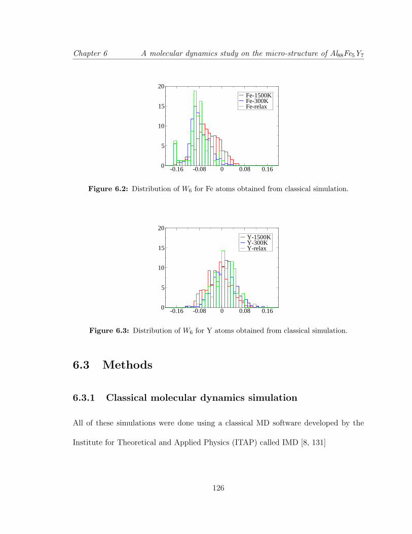
Chapter 6 A molecular dynamics study on the micro-structure of Al88Fe5Y7
-0.16 -0.08 0 0.08 0.160
5
10
15
20
Fe-1500KFe-300KFe-relax
Figure 6.2: Distribution of W6 for Fe atoms obtained from classical simulation.
-0.16 -0.08 0 0.08 0.160
5
10
15
20
Y-1500KY-300KY-relax
Figure 6.3: Distribution of W6 for Y atoms obtained from classical simulation.
6.3 Methods
6.3.1 Classical molecular dynamics simulation
All of these simulations were done using a classical MD software developed by the
Institute for Theoretical and Applied Physics (ITAP) called IMD [8, 131]
126

Chapter 6 A molecular dynamics study on the micro-structure of Al88Fe5Y7
-0.16 -0.08 0 0.08 0.160
2
4
6
8 Al-1500KAl-300KAl-relax
Figure 6.4: Distribution of W6 for Al atoms for VASP run.
-0.16 -0.08 0 0.08 0.160
5
10
15
20
Fe-1500KFe-300KFe-relax
Figure 6.5: Distribution of W6 for Fe atoms for VASP run.
Pair potentials
First, we developed the pair potentials that were used to perform the MD simulations.
This was done by using data from ab-initio calculations on crystalline systems in
which the same elements are in similar environment. The pair potentials for which
the forces and energies were best fit were chosen for use in the IMD simulation. The
fitted energies are shown in Fig. 6.7. The fitted forces are shown in Fig. 6.8. The
127

Chapter 6 A molecular dynamics study on the micro-structure of Al88Fe5Y7
-0.16 -0.08 0 0.08 0.160
5
10
15
20
Y-1500KY-300KY-relax
Figure 6.6: Distribution of W6 for Y atoms for VASP run.
Voronoi 1500K 300K Relax
Types Al Fe Y Al Fe Y Al Fe Y
(0,0,12) 0.28 0.00 0.00 3.55 3.75 0.00 3.98 3.75 0.00
(0,0,12,2) 0.00 0.00 0.00 0.21 0.00 0.00 0.21 0.00 0.00
(0,1,10,2) 0.28 0.00 0.00 1.78 0.00 0.00 2.63 0.00 0.00
(0,3,6,4) 0.65 0.00 0.00 1.35 0.00 0.00 1.42 0.00 0.00
(0,5,4,4) 0.36 0.00 0.00 0.64 0.00 0.00 0.28 0.00 0.00
(0,3,6) 0.00 8.75 0.00 0.00 7.50 0.00 0.00 10.00 0.00
(0,5,4) 0.21 6.25 0.00 0.00 17.50 0.00 0.00 15.00 0.00
Table 6.1: Voronoi statistics for IMD run. The figures show the proportion (percent) of
the important different Voronoi polyhedra.
128

Chapter 6 A molecular dynamics study on the micro-structure of Al88Fe5Y7
Voronoi 1500K 300K Relax
Types Al Fe Y Al Fe Y Al Fe Y
(0,0,12) 0.23 0.00 0.00 0.80 2.00 0.00 1.02 2.00 0.00
(0,0,12,2) 0.11 0.00 0.00 0.00 0.00 0.00 0.00 0.00 0.00
(0,1,10,2) 0.11 0.00 0.00 0.91 0.00 0.00 1.59 0.00 0.00
(0,3,6,4) 0.23 0.00 0.00 0.57 0.00 0.00 1.14 0.00 0.00
(0,5,4,4) 0.91 0.00 0.00 0.23 0.00 0.00 0.45 0.00 0.00
(0,3,6) 0.11 10.00 0.00 0.00 14.00 0.00 0.23 6.00 0.00
(0,5,4) 0.00 12.00 0.00 0.00 22.00 0.00 0.00 20.00 0.00
Table 6.2: Voronoi statistics for VASP run. The figures show the proportion (percent) of
the important different Voronoi polyhedra.
0 50 100 150 200 250 300dE (meV/atom) VASP
0
50
100
150
200
250
300
dE (
meV
/ato
m)
fitte
d
Figure 6.7: Energies fitted with first principles calculations.
129

Chapter 6 A molecular dynamics study on the micro-structure of Al88Fe5Y7
-4 -3 -2 -1 0 1 2 3 4F (eV/Å) VASP
-4
-2
0
2
4
F (
eV/Å
) fit
ted
Figure 6.8: Forces fitted with first principles calculations.
pair potentials that were hence calculated are plotted in Fig. 6.9.
0 2 4 6 8 10r (Å)
-0.2
0
0.2
0.4
0.6
0.8
1
V(r
) (e
V)
AlAlAlFeFeFeYAlYFeYY
Figure 6.9: Pair potentials.
Some initial runs
We prepared a configuration with 200 atoms with the correct density and composition.
We did different trial runs with IMD on this system. We also studied the diffusion
rates at different temperatures and found out that 20 ps were long enough to obtain
130

Chapter 6 A molecular dynamics study on the micro-structure of Al88Fe5Y7
configurations at 1500K which could be treated as independent.
Getting a large system configuration at room temperature
An initial large configuration at 1500K was created by doubling a smaller sized system
(200 atoms) in all the Cartesian directions. The resulting system therefore had 1600
atoms. We then reduced the sizes of the basis vectors so that the volume matched
the low-temperature volume. This system was then allowed to go to a physically
preferred configuration by running it at that temperature for a long time (20.36 ps).
Then, the system was cooled to 600K in 4.072 ps. It was then cooled to 500K in 20.36
ps. The final configuration was obtained by cooling the system to room temperature
(300K) in 4.072 ps. The whole process was repeated 4 more times, each time starting
with the final configuration at 1500K of the previous run and running it for 20.36 ps.
Relaxing the system
We relaxed the last room temperature configuration. The minimum energy configu-
ration was obtained using the conjugate gradient method.
6.3.2 First principles molecular dynamics simulation
The first principles simulations that we performed were done using the Vienna ab-
initio simulation package (VASP) [132–134].
131

Chapter 6 A molecular dynamics study on the micro-structure of Al88Fe5Y7
Getting a room temperature sample
The initial configurations were obtained from IMD runs at 1500K on a systems having
200 atoms. These were allowed to run for 500 fs at 1500K. They were then cooled to
1000K in 500 fs. At this point, each of the simulation cell edge lengths were reduced
by 1% to account for the volume change with temperature. The systems were again
allowed to settle to the new volume for 500 fs. The systems were then cooled to 300K
in 700 fs.
Relaxing the sample
We relaxed the room temperature configurations. The relaxation was done using
VASP which also used the conjugate gradient algorithm.
6.3.3 Analysis
Pair correlation function and Structure factor
The pair correlation function is the normalized density of atoms around a particular
atom. For atom types A and B, it is calculated by first forming a histogram of all
B atoms at a distance between r and r + δr from A atoms. This is then normalized
by dividing by 4πr2δr and nAnB. The resulting function is then smeared with a
Gaussian of standard deviation 0.025A to get the partial pair correlation function for
pair A-B, gAB(r).
132

Chapter 6 A molecular dynamics study on the micro-structure of Al88Fe5Y7
The partial structure factor SAB(q) for pair A-B is obtained from gAB(r) using
SAB(q) = 1 + 4πρ
∫ ∞
0
[gAB(r)− 1]sin(qr)
qrr2dr. (6.1)
The total pair correlation function is obtained from the partials by normalized
weighting in proportion to nAnBZAZB where ZA represents the atomic number of the
A atoms and nA the number of A atoms in the simulation cell. The total structure
factor is also obtained in the same way.
Bond-orientational order parameter W6
The bond-orientational order parameter, W6 [55] helps us detect icosahedral order
present in our system. The value of W6 for an isolated icosahedral cluster is -0.169
which is very different from other clusters [bcc:+0.013; fcc:-0.013; hcp:-0.012]. Thus,
distribution of W6 values in a system can help us in quantifying the amount of icosa-
hedral order.
For a given atom, W6 is calculated as follows. Taking any reference frame, the
orientational angles θ and φ are noted for all the bonds (line joining near neighbor
atoms). The quantity Q6,m = 〈Y6,m(θ, φ)〉 is then calculated for all m, −6 ≤ m ≤ 6,
where the average is taken over all the bonds. From this, W6 is calculated using the
133

Chapter 6 A molecular dynamics study on the micro-structure of Al88Fe5Y7
following.
W6 = (6∑
m=−6
|Q6,m|2)−3/2∑
m1,m2,m3,
m1 +m2 +m3 = 0
6 6 6
m1 m2 m3
Q6,m1Q6,m2Q6,m3(6.2)
where
6 6 6
m1 m2 m3
represent the Wigner 3j symbols.
Voronoi analysis
Voronoi analysis helps us in visualizing the local environments around atoms. For
this, first a Voronoi polyhedron is constructed around a chosen atom in the following
way. Perpendicularly bisecting planes are drawn for all lines joining that atom to
other atoms. The smallest closed polyhedron thus formed is the Voronoi polyhedron
for this atom. It is then assigned a set of integers (F3, F4, F5, ...) where Fi is
the number of faces of the Voronoi polyhedron with i edges. For example, (0,0,12)
represents the icosahedron, (0,12,0) represents the fcc and hcp, (0,6,0,8) represents
the bcc, and so on. (0,0,12,x), x = 2, 3, 4, ... represents icosahedral structures with
disclinations.
134

Chapter 6 A molecular dynamics study on the micro-structure of Al88Fe5Y7
Honeycutt-Anderson analysis
This is another method to characterize and quantify local order. Each bond between
to atoms of types A and B is characterized by 3 integers n1n2n3, where n1 is 1 if the
atoms are nearest neighbors, 2 if they are second neighbors and so on (We are not
interested in n1 > 2); n2 is the number of common neighbors the two atoms have;
and n3 is the number of pairs of these common neighbors which are neighbors of each
other. For example, 155 is characteristic of perfect icosahedra, 244 is present in bcc
structures, 233 is present when an atom sits outside an icosahedron at second neighbor
distance from the center atom, and so on. [Note: The distances corresponding to near
neighbors, second neighbors, and so on, are obtained from the minima in the gAB(r)
plot.]
6.4 Observations and inference
The total and partial pair correlation functions obtained from the classical molecular
dynamics simulation has been plotted in Fig. (6.10). The structure factor was calcu-
lated from this and plotted in Fig. 6.11. A comparison with X-ray diffraction data
has been shown in Fig. 6.12.
The pair correlation functions obtained from first principles MD simulation has
been plotted in Fig. 6.13. The structure factors obtained from these has been shown
in Fig. 6.14. It is to be noted, however, that due to the smallness of the system
135

Chapter 6 A molecular dynamics study on the micro-structure of Al88Fe5Y7
1 2 3 4 5 6 7 8 9 10r (Å)
0
0.5
1
1.5
2
2.5
3
g(r)
AlAlAlFeAlYFeFeFeYYYTotal
Figure 6.10: Total and partial pair correlation functions from the classical MD simula-
tions.
1 2 3 4 5 6 7 8 9 10
q (Å-1
)
0
0.5
1
1.5
2
2.5
3
S(q
)
AlAlAlFeAlYFeFeFeYYYTotal
Figure 6.11: Total and partial structure factors obtained from classical simulation.
size, the total structure factor in Fig. 6.14 does not agree well with diffraction data.
The range of wave-vectors for which diffraction data was available to us made us
decide that it was more justified to compare the pair correlation functions obtained
by Fourier transforming the diffraction data with those calculated using first principles
simulation. Such a comparison is shown in Fig. 6.15.
136

Chapter 6 A molecular dynamics study on the micro-structure of Al88Fe5Y7
0 1 2 3 4 5 6 7 8 9 10
q (Å-1
)
0
1
2
3
4
S(q
)
experimentIMD
Figure 6.12: Comparison of total structure factors from experiment and classical MD
simulation.
1 2 3 4 5 6 7r (Å)
0
0.5
1
1.5
2
2.5
g(r)
AlAlAlFeAlYFeFeFeYYYTotal
Figure 6.13: Total and partial pair correlation functions obtained from ab-initio simula-
tion.
6.4.1 A look at the Al-Fe-Y phase diagram
The coexisting phases of Al-Fe-Y that may be present in our system are Al10Fe2Y.oC52,
pure Al as Al.cF4 and an Al-Y binary as Al3Y.hP8 [Fig. 6.16]. The Al8CeFe2.oP44
137

Chapter 6 A molecular dynamics study on the micro-structure of Al88Fe5Y7
1 2 3 4 5 6 7 8 9 10
q (Å-1
)
0
1
2
3
S(q
)
AlAlAlFeAlYFeFeFeYYYTotal
Figure 6.14: Total and partial structure factors obtained from ab-initio simulation.
1 2 3 4 5 6 7r (Å)
0
0.5
1
1.5
2
2.5
g(r)
VASPexperiment
Figure 6.15: Comparison of pair correlation function from first principles simulation and
Fourier transforming X-ray diffraction data.
and Al10Fe2Gd.oC52 [Gd can be replaced by Y] phases are theoretically predicted to
be stable but are not yet experimentally verified.
We looked at the environments of Fe-Y and Y-Y in the Al10Fe2Y crystal. In
[Fig. 6.17], we see that Y-Y are second neighbors and there are 3 common Al neighbors
which form a square (approximately). Presence of such a structure could be studied
138

Chapter 6 A molecular dynamics study on the micro-structure of Al88Fe5Y7
0.9
0.8
0.7
0.6
0.5
0.6
0.7
0.8
0.9 0.9
0.8
0.7
0.6
0.5
0.6
0.7
0.8
0.9
0.9 0.8 0.7 0.6 0.5 0.6 0.7 0.8 0.9
12
5
34
Al
Fe
Y
1 Al10
Fe2Gd.oC52 (-372)
2 Al8CeFe
2.oP44 (-413)
5 Al8Fe
4Y.tI26 (-442)
3 Al23
Ni6Y
4.mC66 (50)
4 Al9Co
3Y
2.oC56 (22)
stable (∆H) unstable (∆E>20)
Figure 6.16: Al-Fe-Y phase diagram. Phases 2 and 3 are theoretically predicted to be
stable but have not been found experimentally.
with Honecutt-Anderson (HA) analysis and looking for HA index 244 where the first
2 stands for second neighbors, the first 4 indicates 4 common neighbors and the last
4 shows the number of bonds between the common neighbors.
In [Fig. 6.18], we see that Fe-Y are second neighbors and there are 3 Al atoms which
form an approximately equilateral triangle which are very close to being immediate
neighbors for both Fe and Y. Such a structure would correspond to HA index of 233
if the Al atoms were indeed common neighbors. However, this structure could also be
interpreted as an icosahedron with Fe as the centre atom and Al as the surrounding
atoms and a Y atom outside this.
139

Chapter 6 A molecular dynamics study on the micro-structure of Al88Fe5Y7
Figure 6.17: Y-Y environment in Al10Fe2Y . Grey atoms represent Al, blue represent Fe
and purple represent Y.
Figure 6.18: Y-Y environment in Al10Fe2Y . Grey atoms represent Al, blue represent Fe
and purple represent Y.
140

Chapter 6 A molecular dynamics study on the micro-structure of Al88Fe5Y7
6.4.2 Honeycutt-Anderson analysis
The distribution of the HA indices for the bonds in the configurations obtained from
both classical and ab-initio simulations also show the increased icosahedral order in
the cooled and relaxed configurations. These are plotted in Figs. 6.19–6.28.
100 120 140 160 180 2000
0.05
0.1
0.15
0.2
0.25AlAl-1500KAlAl-300KAlAl-relax
Figure 6.19: Statistics for nearest neighbor HA indices for Al-Al pairs obtained from clas-
sical simulation.
100 120 140 160 180 2000
0.1
0.2
0.3
0.4
0.5
0.6 AlFe-1500KAlFe-300KAlFe-relax
Figure 6.20: Statistics for nearest neighbor HA indices for Al-Fe pairs obtained from clas-
sical simulation.
141

Chapter 6 A molecular dynamics study on the micro-structure of Al88Fe5Y7
100 120 140 160 180 2000
0.1
0.2
0.3
0.4
AlY-1500KAlY-300KAlY-relax
Figure 6.21: Statistics for nearest neighbor HA indices for Al-Y pairs obtained from clas-
sical simulation.
100 120 140 160 180 2000
0.1
0.2
0.3
0.4
0.5
FeY-1500KFeY-300KFeY-relax
Figure 6.22: Statistics for nearest neighbor HA indices for Fe-Y pairs obtained from clas-
sical simulation.
Some second neighbor HA indices which we thought were interesting to look at
were 244 for Y-Y pairs and 233 for Fe-Y pairs.
For the Y-Y pairs [Figs. 6.29 and 6.30], we see that 244 is preferred by the IMD
configuration but not by the VASP configuration. Since 244 for Y-Y is a characteristic
of the crystal structure, we conclude that the VASP run did a better job at going to
142

Chapter 6 A molecular dynamics study on the micro-structure of Al88Fe5Y7
100 120 140 160 180 2000
0.05
0.1
0.15
0.2
0.25
0.3 YY-1500KYY-300KYY-relax
Figure 6.23: Statistics for nearest neighbor HA indices for Y-Y pairs obtained from clas-
sical simulation.
100 120 140 160 180 2000
0.05
0.1
0.15
0.2
0.25AlAl-1500KAlAl-300KAlAl-relax
Figure 6.24: Statistics for nearest neighbor HA indices for Al-Al pairs obtained from first
principles simulation.
the amorphous structure.
For the Fe-Y pairs [Figs. 6.31 and 6.32], we see that the 233 is preferred by VASP
and not by IMD.
143

Chapter 6 A molecular dynamics study on the micro-structure of Al88Fe5Y7
100 120 140 160 180 2000
0.1
0.2
0.3
0.4
0.5AlFe-1500KAlFe-300KAlFe-relax
Figure 6.25: Statistics for nearest neighbor HA indices for Al-Fe pairs obtained from first
principles simulation.
100 120 140 160 180 2000
0.05
0.1
0.15
0.2
0.25AlY-1500KAlY-300KAlY-relax
Figure 6.26: Statistics for nearest neighbor HA indices for Al-Y pairs obtained from first
principles simulation.
6.4.3 Bond orientation
The distribution of W6 values becomes more skewed on cooling and further on re-
laxing, towards the value for the perfect icosahedron (-0.169) for Al and Y centered
analysis for both IMD and VASP runs. There is no such trend in the Y centered W6
distribution.
144

Chapter 6 A molecular dynamics study on the micro-structure of Al88Fe5Y7
100 120 140 160 180 2000
0.1
0.2
0.3
0.4
0.5
FeY-1500KFeY-300KFeY-relax
Figure 6.27: Statistics for nearest neighbor HA indices for Fe-Y pairs obtained from first
principles simulation.
100 120 140 160 180 2000
0.1
0.2
0.3
0.4
YY-1500KYY-300KYY-relax
Figure 6.28: Statistics for nearest neighbor HA indices for Y-Y pairs obtained from first
principles simulation.
6.4.4 Voronoi analysis
The Voronoi polyhedron representing the perfect icosahedron is (0, 0, 12). For the
IMD simulation (Table 6.1), Voronoi analysis indicated that the proportion of Al
centered icosahedra increased on cooling, and increased further on relaxing. Fe cen-
145

Chapter 6 A molecular dynamics study on the micro-structure of Al88Fe5Y7
200 220 240 260 280 3000
0.05
0.1
0.15
0.2
0.25YY-relaxYY-1500KYY-300K
Figure 6.29: Statistics for second neighbor HA indices for Y-Y pairs obtained from clas-
sical simulation.
200 220 240 260 280 3000
0.05
0.1
0.15
0.2
0.25YY-relaxYY-1500KYY-300K
Figure 6.30: Statistics for second neighbor HA indices for Y-Y pairs obtained from ab-
initio simulation.
tered icosahedra also increased in number on cooling but did not change on relaxing.
An Y atom is too big to form an icosahedron with it at the center and Al atoms
around.
For the VASP run (Table 6.2), the trends were exactly same as the IMD run. The
numbers however, were much less in this case.
146

Chapter 6 A molecular dynamics study on the micro-structure of Al88Fe5Y7
200 220 240 260 280 3000
0.1
0.2
0.3
0.4
FeY-relaxFeY-1500KFeY-300K
Figure 6.31: Statistics for second neighbor HA indices for Fe-Y pairs obtained from clas-
sical simulation.
200 220 240 260 280 3000
0.1
0.2
0.3
0.4
FeY-relaxFeY-1500KFeY-300K
Figure 6.32: Statistics for second neighbor HA indices for Fe-Y pairs obtained from ab-
initio simulation.
147

Chapter 7
Detecting hidden structures in
metallic glasses by multiresolution
network clustering
7.1 Introduction
This chapter introduces a new method of obtaining the essential structural features
on all length scales in general complex systems with the knowledge of pairwise inter-
action strengths. We apply our methods to detect the natural scales and obtain the
structures of metallic glasses. Complex systems and glasses are not easy to analyze
with conventional theoretical tools.[135] In a gas, all interactions between the basic
constituents are weak, so the system is easy to understand and analyze. At the other
148

Chapter 7 Multiresolution network clustering
extreme, the interactions in regular periodic solids are generally strong, and such
solids may be characterized by their unit cells and related broken symmetries.
The situation is radically different for liquids and glasses. Liquids that are rapidly
cooled (“supercooled”) below their melting temperature cannot crystallize and in-
stead, at sufficiently low temperatures, become “frozen” in an amorphous state (a
“glass”) on experimental time scales. On supercooling, liquids may veer towards lo-
cal low energy structures,[130, 136] such as icosahedral structures observed in metallic
glasses,[137, 138] before being quenched into the amorphous state. Lacking a simple
crystalline reference, the general structure of glasses is notoriously difficult to quantify
in a meaningful way beyond the smallest local scales. As such, it remains a paradigm
for analyzing structure in complex materials.
Network analysis has been transformative in generating keen new insights in nu-
merous areas such as sociology, homeland security, biology, and many other problems.
Complex physical problems have not yet been examined before through this prism in
this detail. We specifically introduce methods from the growing discipline of “com-
munity detection”.[139] The key idea is that any complex physical system may be
expressed as a network of nodes (e.g., atoms, electrons, etc.) and connecting links
that quantify the relations (interactions/correlations) between the nodes. With this
representation, we then apply multiresolution methods [6] from network theory to
analyze the systems.
149

Chapter 7 Multiresolution network clustering
7.1.1 Partitions of large systems into weakly coupled ele-
ments
As depicted in Fig. 7.1, community detection describes the problem of finding clusters
(“communities”) of nodes with strong internal connections and weak connections
between different clusters. The definitions of nodes and edges depend on the system
being modeled. For the present system, between each pair of nodes i and j we have
an edge weight Vij which may emulate an interaction energy or measured correlation
between sites i and j. The nodes may belong to any of q communities, {Ca}qa=1. In
our particular realization, the nodes represent particles and edges model the pair-wise
potential energy interactions.
7.1.2 Community detection method
Our (Potts type) Hamiltonian reads
H =1
2
q∑
a=1
∑
i,j∈Ca
(Vij − v)[θ(v − Vij) + γθ(Vij − v)]. (7.1)
In Eq. (7.1), the inner sum is over nodes i and j in the same community Ca, and the
outer sum is performed over the q different communities. The number of communities
q may be specified from the outset or left arbitrary (the usual case) allowing the
algorithm to determine q based on the lowest energy solution(s).[6, 140]
Minimizing this Hamiltonian corresponds to identifying strongly connected clus-
ters of nodes. The parameter γ > 0 tunes the relative weights of the connected and
150

Chapter 7 Multiresolution network clustering
Figure 7.1: A weighted network with 4 natural (strongly connected) communities. The
goal in community detection is to identify such strongly related clusters of
nodes. Solid lines depict weighted links corresponding to complimentary or
attractive relationships between nodes i and j (denoted by Aij) [(Vij − v) < 0
in Eq. (7.1)]. Gray dashed lines depict missing or repulsive edges (denoted by
Bij) [(Vij − v) > 0]. In both cases, the relative link weight is indicated by the
respective line thicknesses.
unconnected edges and allows us to vary the targeted scale of the community division
(the “resolution”). The model for the current application could be further generalized
by incorporating n-body interactions or correlation functions (such as three or four
point correlation functions). Details concerning a greedy minimization of Eq. (7.1)
appear in Refs. [6] and [140].
151

Chapter 7 Multiresolution network clustering
7.1.3 Multiresolution network analysis
We address multi-scale partitioning [6] by employing information-theory measures
[141, 142] to examine contending partitions for each system scale. While decreasing γ,
we minimize Eq. (7.1) resulting in partitions with progressively lower intra-community
edge densities, effectively “zooming out” toward larger structures. A key construct
in our approach is the application of replicas – independent solutions of the same
problem. The number of replicas p may be set by the user where higher value of p
leads to more accurate analysis.
In static systems replicas were formed by permuting the order of nodes in Ref.
[6]. In this work, we take advantage of the dynamic system to implement a further
generalization where replicas are defined at different times (see Fig. 7.2. We au-
tomatically determine the natural scales of a system by identifying the values of γ
for which these replicas agree most strongly via information theory measures such as
normalized mutual information NMI and variation of information VI.
The central result from Ref. [6], that we use in this work, is that extrema (includ-
ing plateaux) of information theory overlaps (when averaged over all replica pairs) in-
dicate the “natural” network scales.[6] That is, we find the values γ∗ for which the av-
erage Q of information overlaps (over all replica pairs) is extremal, (dQ/dγ)|γ=γ∗ = 0.
We then identify the parititions that correspond to these γ∗(s).
152

Chapter 7 Multiresolution network clustering
Figure 7.2: A set of replicas separated by a time ∆t between successive replicas. We gen-
erate a model network for each replica using the potential energy between the
atoms as the respective edge weights and then solve each replica independently
by minimizing Eq. (7.1) over a range of γ values. We then use information
measures [6] to evaluate how strongly pairs of replicas agree on the ground
states of Eq. (7.1).
7.2 Systems studied
We examine a model glass former derived from the three-component AlYFe metallic
glass of Chapter 6 which we designate as “A”, “B”, and “C” in mixture ratios of
88%, 7%, and 5%, respectively. We additionally test the ubiquitous Lennard-Jones
potential using the Kob-Andersen (KA) 80:20 binary liquid [9] which lies in the glass-
forming mixture region [143].
153

Chapter 7 Multiresolution network clustering
7.2.1 Ternary model glass former
In this section, we discuss our study on the ternary system mentioned above. As
depicted in Fig. 7.4, we use classical molecular dynamics (MD) [8] to simulate the
system dynamics.
a0 a1 a2 a3 a4 a5
AA * * * * * *
AB 1.92 17.4 6.09 3.05 -4.68 3.48
AC 2.38 8.96 -14.9 3.11 -3.88 4.38
BB * * * * * *
BC 1.88 8.00 -3.42 2.53 -1.25 3.00
CC * * * * * *
Table 7.1: Fit parameters for Eq. (7.2) obtained from fitting configuration forces and
energies to ab-initio data (as in Chapter 6). The units of the parameters are
such that given r in A, φ(r) is in eV . (That is, the parameters a1, a4 and a5
are dimensionless, a0 is in A, a2 is in eV Aa5 and a3 is in A−1.) The same-
species (*) data is replaced by a suggested potential derived from generalized
pseudo-potential theory [7].
For this, as in Chapter 6, we need accurate effective pair potentials that portray
the pairwise interactions between the atoms in the system. Our model potential
154

Chapter 7 Multiresolution network clustering
Figure 7.3: The pair potentials for our three-component model glass former (see Fig.
7.4). We indicate the atomic types by “A”, “B”, and “C” which are included
with mixture ratios of 88%, 7%, and 5%, respectively. The units are given
for a specific candidate atomic realization (AlYFe) discussed in the text. The
same-species data uses a suggested potential derived from generalized pseudo-
potential theory [7].
energy function is,
φ(r) =(a0r
)a1+a2ra5
cos (a3r + a4) , (7.2)
where r is the distance between the centers of two atoms. This potential form incor-
porates a realistic weak long range interaction. Table 7.1 summarizes the parameter
values ai which depend on the specific types for a pair of interacting atoms, and Fig.
7.3 shows the respective potential plots.
After the forces and energies were fit to first-principles data (as in Chapter 6, the
same-species model interactions are finally replaced by that suggested by generalized
155

Chapter 7 Multiresolution network clustering
Figure 7.4: A depiction of our simulated model glass former with three components “A”,
“B”, and “C” with mixture ratios of 88%, 7%, and 5%, respectively. The
N = 1600 atoms are simulated via IMD [8] in cube of approximately 31 A
in size with periodic boundary conditions. The identities of the atoms are C
(red), A (silver), B (green) in order of increasing diameters.
pseudo-potential theory (GPT).[7] As illustrated in Fig. 7.4, we simulate N = 1600
atoms in a cubic system approximately 31 A in size using periodic boundary condi-
tions. This width is approximately twice the size of any suspected MRO structures.
The system is initialized at a temperature of T = 1500 K and allowed to equilibrate
for a long time using a constant number of atoms (N), a constant volume (V), and a
constant energy (E). That is, we work within the NVE ensemble. After allowing for
system equilibration, we save s high temperature configurations separated by a fixed
156

Chapter 7 Multiresolution network clustering
period of simulation time. (We fixed the value of s at 12 for all our simulations.)
Prior to cooling, the length scales in the system are changed by 1% to account for
the increase in density as a result of cooling since we choose to cool the system in an
NVT ensemble to control the temperature. This was done to keep a realistic density
difference between the high and low temperature configurations. It should not have
any important physical consequences pertaining to local structure. The system is then
rapidly quenched to a temperature of T = 300 K, and it is allowed to equilibrate (in a
mostly frozen state) in an NVE ensemble. We again save s separate low temperature
configurations separated by a long period of simulation time.
7.2.2 Lennard-Jones glass
Here we discuss the application of our methods to simulations of the Kob-Anderson
mixture. The pair potentials are given by
φαβ(r) = 4ǫαβ
[
(σαβr
)12
−(σαβr
)6]
(7.3)
where α or β designate one of two atomic types A and B. Specifically, in accord with
KA we set the dimensionless units ǫAA = 1.0, ǫAB = 1.5, ǫBB = 0.5, σAA = 1.0,
σAB = 0.80, and σBB = 0.88.
As in the ternary glassy system above, we use MD [8] to simulate a LJ system of
N = 2000 atoms. The system is initialized at a temperature of T = 5 (using energy
units where the Boltzmann constant kB = 1) and allowed to evolve for a long time.
157

Chapter 7 Multiresolution network clustering
We save s high temperature configurations separated by 10000 time steps. The time
step size is ∆t = 0.0069 in LJ time units. Then, the system is rapidly quenched to a
temperature of T = 0.01 which is well below the glass transition temperature of the
KA-LJ system. The system is evolved in this mostly frozen state, and we save s low
temperature configurations separated by 10000 steps of simulation time.
7.3 Results
We assign edges between the nodes (atoms) with the respective weights based on the
empirical pair-potentials given by Eqs. (7.2) and (7.3). Specifically, we calculate the
potential energy φij between each pair of nodes i and j in the system and then shift
each value by a constant φ0 to obtain φ′ij = φij + φ0 (assuming that φij → 0 as the
distance between particles i and j tends to infinity (r → ∞)). The shift φ0 > 0 is
necessary for the community detection algorithm to properly partition the network
of atoms since it provides an objective definition of which interatomic spacings are
preferable for a well-defined cluster and which are preferred to be excluded from a
cluster.
In our particular application here, we calculate the average potential energy of
the system and set φ0 = −φavg. For use in Eq. (7.1), we define an edge with a weight
Aij = −φ′ij between nodes i and j if φ′
ij < 0, and we weight any missing links (or
“repulsive edges”) by Bij = φ′ij if φ
′ij ≥ 0. We then solve both model systems over a
158

Chapter 7 Multiresolution network clustering
large range of γ using s = 12 replicas and t = 10 optimization trials per replica.
While φ0 = −φavg is an intuitive shift that accomplishes the goal of an objective
cluster definition here, it is not an appropriate shift for some problems. For example,
using φ0 = −φavg turns out to be problematic in some cases for lattice models. In a
general setting, we examine a continuum of potential shifts φ0 and monitor extrema
in the information theory measures as a function of both γ in Eq. (7.1) and φ0.
In addition to the systems tested below, we applied the algorithm to various test
cases including square, triangular, and cubic lattice structures. The algorithm is able
to correctly identify the natural leading order scales (plaquettes and composites of
plaquettes as “cascades” in the information theory correlations). Further testing in-
volved two-dimensional defects (dislocations, interstitials, etc.) and domain walls in
a lattice. Defects in triangular lattices occurred most frequently near cluster bound-
aries.
We also tested static configurations for the ternary model glass system where each
replica is a model of the same configuration. There we detected structures in both
low and high temperatures where the high temperature “structures” are more fragile
(that is, harder to solve in the clustering problem). This corresponds to identifying
relevant transient features in a dense liquid.
159

Chapter 7 Multiresolution network clustering
7.3.1 Ternary model glass results
In Figs. 7.5 and 7.6, panels (a) and (b) show the information theory based correlations
(averaged over all replica pairs as in [6]) over a range of network resolutions.
Figure 7.5: Panels (a) and (b) show the plots of information measures IN , V , H, and I
and the number of clusters q (right-offset axes) versus the Potts model weight
γ in Eq. (7.1). The ternary model system contains 1600 atoms in a mixture of
88% type A, 7% of type B, and 5% of type C with a simulation temperature
of T = 300 K which is well below the glass transition for this system. This
system shows a strongly correlated set of replica partitions as evidenced by
the information extrema at (i) in both panels. A set of sample clusters for
the best resolution at γ ≃ 0.001 is depicted in Fig. 7.9.
160

Chapter 7 Multiresolution network clustering
Figure 7.6: Panels (a) and (b) show the plots of information measures IN , V , H, and I
and the number of clusters q (right-offset axes) versus the Potts model weight
γ in Eq. (7.1). The ternary model system contains 1600 atoms in a mixture of
88% type A, 7% of type B, and 5% of type C with a simulation temperature
of T = 1500 K which is well above the glass transition for this system. At this
temperature, there is no resolution where the replicas are strongly correlated.
See Fig. 7.5 for the corresponding low temperature case where the replicas are
much more highly correlated at γ ≃ 0.001.
The lower temperature system at T = 300 K in Fig. 7.5(a) shows a peak NMI at
(ia) with a corresponding VI minimum at (ib). Fig. 7.7 depicts an example of the
full system partition.
161

Chapter 7 Multiresolution network clustering
Figure 7.7: A depiction of the full partitioned system where unique cluster memberships
are depicted as distinct colors (best viewed in color). The atomic identities
are B, A, C in order of increasing diameters. Overlapping nodes (multiple
memberships per node) are added to these communities to determine the best
interlocking system clusters.
Fig. 7.8 shows some sample clusters within the simulation bounding box at resolu-
tion parameter value of γbest ≃ 0.001 where we include overlapping node memberships
(the replicas correlations are calculated on partitions), and Fig. 7.9 depicts additional
samples of the best clusters.
The corresponding high temperature (T = 1500 K) solutions have a much lower
NMI at γbest ≃ 0.001 indicating significantly worse agreement among replicas. That
is, one would expect that the high temperature system T = 1500 K is in a liquid state,
162
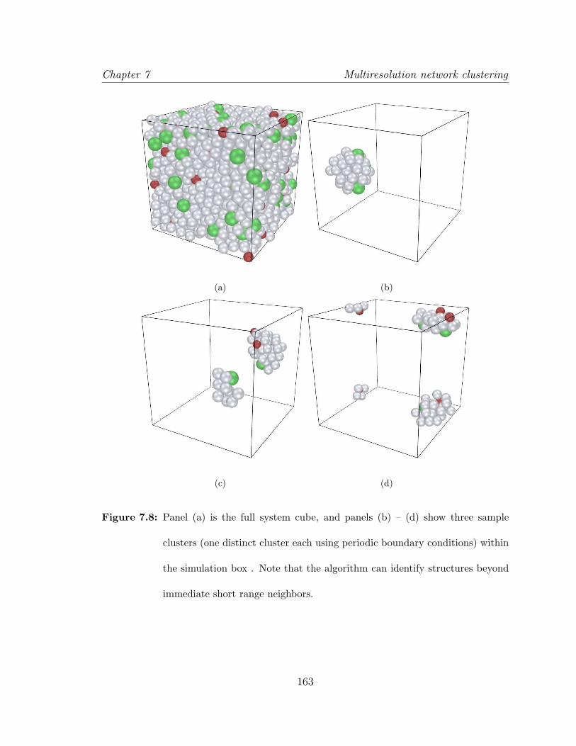
Chapter 7 Multiresolution network clustering
(a) (b)
(c) (d)
Figure 7.8: Panel (a) is the full system cube, and panels (b) – (d) show three sample
clusters (one distinct cluster each using periodic boundary conditions) within
the simulation box . Note that the algorithm can identify structures beyond
immediate short range neighbors.
163

Chapter 7 Multiresolution network clustering
Figure 7.9: A depiction of some of the best clusters of the low temperature (T = 300K)
ternary system at the peak replica correlation at feature (i) in Fig. 7.5. These
clusters include overlapping node membership assignments where each node
is required to have an overall negative binding energy to the other nodes in
the cluster. The atomic identities are C (red), A (silver), B (green) in order
of increasing diameters.
so any observed features are not dynamically stable across all replicas (snapshots of
the system over time). At T = 300 K, the best structures have consistent cluster
sizes that are exclusively MRO.
The plateau regions for γ > 10 are similar to the LJ plot in Fig. 7.10, but in this
system the NMI plateau is lower. In the high temperature case in Fig. 7.6, there are
additional “almost-plateaus” for the range 0.001 . γ . 0.1. These plateaus represent
a region of structural transition, but we are not concerned with them because the
164

Chapter 7 Multiresolution network clustering
replica correlations are very low.
Figure 7.10: Panels (a) and (b) show the plots of information measures IN , V , H, and
I and the number of clusters q (right-offset axes) versus the Potts model
weight γ in Eq. (7.1). The LJ system contains 2000 atoms in a mixture of
80% type A and 20% type B (Kob-Andersen binary LJ system [9]) with a
simulation temperature of T = 0.01 (energy units) which is well below the
glass transition of Tc ≃ 0.5 for this system. This system shows a somewhat
strongly correlated set of replica partitions as evidenced by the information
extrema at (ia,b) in panels (a) and (b). A set of sample clusters for the best
resolution at γ = 104 is depicted in Fig. 7.11.
165

Chapter 7 Multiresolution network clustering
Figure 7.11: Several of the best clusters for the peak replica correlation at feature (i) in
Fig. 7.10. These clusters include overlapping node membership assignments
where each node is required to have a overall negative binding energy to the
other nodes in the cluster. The atomic identities are B (silver) and A (red)
in order of increasing diameters.
7.3.2 Binary Lennard-Jones glass results
In Figs. 7.10 and 7.12, panels (a) and (b) show the data for the replica information
correlations over a range of network resolutions. The lower temperature system at
a temperature of T = 5 (in units of kB = 1) in Fig. 7.5(a) shows a plateau in
NMI at (ia) with a corresponding VI plateau at (ib) which are the local extrema
(V = 0 is a trivial solution with only one cluster in this problem). Fig. 7.11 depicts
a sample of the best clusters, including overlapping node memberships, at resolution
(i) for γbest ≃ 104. The corresponding higher temperature solutions at γbest ≃ 104
166

Chapter 7 Multiresolution network clustering
Figure 7.12: Panels (a) and (b) show the plots of information measures IN , V , H, and
I and the number of clusters q (right-offset axes) versus the Potts model
weight γ in Eq. (7.1). The LJ system contains 2000 atoms in a mixture of
80% type A and 20% type B (Kob-Andersen binary LJ system [9]) with a
simulation temperature of T = 5 (energy units) which is well above the glass
transition of Tc ≃ 0.5 for this system. At this temperature, the replicas are
significantly less correlated than the corresponding low temperature case in
Fig. 7.10.
(see Figs. 7.12 and7.13) have a lower NMI (indicating a weak agreement among
replicas). The dependence number of replicas (See Fig. 7.13) required to achieve
high accuracy underscores the faint agreement between contending solutions and the
167

Chapter 7 Multiresolution network clustering
(a) (b) (c) (d)
Figure 7.13: A sample depiction of dispersed clusters for the LJ system Eq. (7.3) at a tem-
perature of T = 5 (in units where kB = 1). The shown clusters correspond
to the multiresolution plot in Fig. 7.12 at value of the resolution parameter
of γ = 104. These clusters are a sample of high temperature counterparts to
the low temperature clusters in Figs. 7.10 and 7.11. Panels (a) and (b) show
a more typical example of dispersed clusters at a number of replicas s = 10.
In some cases, the identified high temperature clusters can be more com-
pact, but not densely packed. Panels (c) and (d) provide sample solutions
for s = 20 replicas.
high temperature complexity of the problem. Our identified structures for this LJ
model system are consistent in terms of the cluster sizes and are almost exclusively
SRO configurations with simple adjunct-type atoms extending into the low end of
MRO size structures.
168

Chapter 7 Multiresolution network clustering
7.4 Conclusions
Our method is a new and very general approach to determine the natural multi-scale
structures of complex physical systems. We do not bias the expected configurations
in any way. The only required inputs are the pairwise interaction potentials between
the atoms. In case information about such pairwise interactions are not easy to
obtain, the algorithm can be used with the pair correlation functions used as weights.
Information theory extrema (including plateaus) between contending solutions give
the different pertinent structures on all important length scales (lattice scales and
correlation lengths) of the system in an unbiased unified way.
169
Appendix
A High temperature series expansion of the cor-
relation function
We now outline in detail how we may obtain a high temperature (T ) series expansion
of the correlation function to arbitrary order for a general system with translational
invariance. The results we present below are valid in the high temperature phase of
general lattice (spin or other) and continuum systems. However, these may hold at
low temperatures, provided we can analytically continue to low temperatures from the
high temperature phase, i.e., arrive at these without having a phase transition. We
should emphasize that as we set the temperature to be arbitrarily high, the density
does not have to be small as is assumed in methods derived from Mayer’s cluster
expansion for fluids. Our result is therefore valid for the high temperature phase
of any system. Albeit trivial, we should remark that, formally, for any finite size
system of N sites (or of finite volume for a continuum theory), no matter how large
170

Appendix
yet still finite, there are no phase transitions [instead there might be progressively
sharp (as N increases), yet analytic, crossovers]. Thus, in finite size systems, the
radius of convergence of the high T expansion is infinite. In general, the long range
character of the interactions will not enable us to invoke many of the simplifying
elegant tricks presented elsewhere. For instance, the counting of connected contours
and loops [144, 145] that appear in high temperature series expansions involving
nearest neighbor interactions cannot be applied here.
We can perform the high temperature series expansion directly in the original spin
space. However, we find it easier to make a transformation to a dual space where our
Boltzmann weights become Gaussian in the high temperature limit.
The correlation function of the original theory can be expressed in terms of the
correlation function (and higher moments) of the dual theory – we employ that in
our calculation. The dual theory to a nearest neighbor ferromagnetic system is a
Coulomb gas. A nearest neighbor ferromagnetic system in dimensions d > 2 at
low T has an ordered phase and a small correlation length (the correlation length
diverges at T = Tc). This does not imply that the Coulomb system has a small
correlation length at high temperature. O(n) constraints become faint at high T in
the dual theory whereas in the exact Coulomb gas at high T , the O(n) constraints
are there. The same also applies for a soft spin realization of the Coulomb gas where
exp[−βu(S2− 1)2] which is zero as β → ∞ (or T → 0) unless S2 = 1 everywhere. By
contrast in the exact dual theory at high temperature, the relative strength of theO(n)
171

Appendix
constraints becomes negligible relative to the “interaction” term containing (βV )−1.
Even though we can ignore β prefactors when β = O(1) and consider dual theories
and soft spin realization we cannot ignore the T dependence at high T about the
infinite T disordered limit. Otherwise we get a contradiction as our exact calculation
with the exact dual theory (containing the T -dependent prefactors) shows.
We will keep things general and perform the simple series expansion of the dual
Hamiltonian Hd in Eq. (3.6):
Hd = −N2
2β2
∑
~x,~y
V −1(~x− ~y)~η(~x) · ~η(~y)
− 1
β
∑
~x
ln
(
In/2−1(√nN |~η(~x)|)
(√nN |~η(~x)|)n/2−1
)
,
= −N2
2β2
∑
~x,~y
V −1(~x− ~y)~η(~x) · ~η(~y)
−N2
2β
∑
~x
~η(~x) · ~η(~x)
+N4
4(n+ 2)β
∑
~x
[~η(~x) · ~η(~x)]2 + ... . (A-4)
In Eq. (A-4), the interaction V should be thought of as a translationally invariant
matrix. That is, in a Dirac type notation, 〈~x|V |~y〉 = V (~x− ~y). In Eq. (A-4), V −1 is
the inverse Fourier transform of 1/v(~k), where v(~k) is the Fourier transform of V (~x)
[146].
Next, we separate Hd into a quadratic part Hd0 and higher order (interaction
172
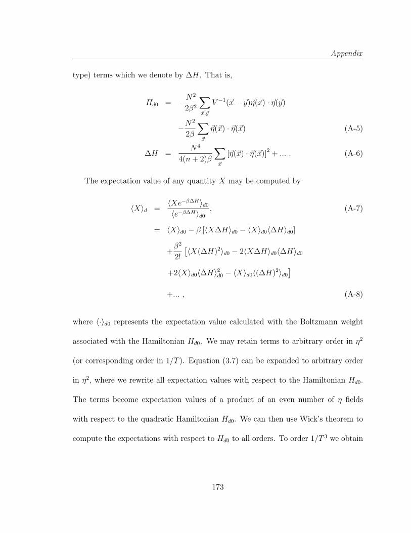
Appendix
type) terms which we denote by ∆H. That is,
Hd0 = −N2
2β2
∑
~x,~y
V −1(~x− ~y)~η(~x) · ~η(~y)
−N2
2β
∑
~x
~η(~x) · ~η(~x) (A-5)
∆H =N4
4(n+ 2)β
∑
~x
[~η(~x) · ~η(~x)]2 + ... . (A-6)
The expectation value of any quantity X may be computed by
〈X〉d =〈Xe−β∆H〉d0〈e−β∆H〉d0
, (A-7)
= 〈X〉d0 − β [〈X∆H〉d0 − 〈X〉d0〈∆H〉d0]
+β2
2!
[
〈X(∆H)2〉d0 − 2〈X∆H〉d0〈∆H〉d0
+2〈X〉d0〈∆H〉2d0 − 〈X〉d0〈(∆H)2〉d0]
+... , (A-8)
where 〈·〉d0 represents the expectation value calculated with the Boltzmann weight
associated with the Hamiltonian Hd0. We may retain terms to arbitrary order in η2
(or corresponding order in 1/T ). Equation (3.7) can be expanded to arbitrary order
in η2, where we rewrite all expectation values with respect to the Hamiltonian Hd0.
The terms become expectation values of a product of an even number of η fields
with respect to the quadratic Hamiltonian Hd0. We can then use Wick’s theorem to
compute the expectations with respect to Hd0 to all orders. To order 1/T 3 we obtain
173

Appendix
for ~x 6= 0,
G(~x) = −V (~x)
kBT+
1
(kBT )2
[
∑
~z
V (~z)V (~x− ~z)− 2V (0)V (~x)
]
+1
(kBT )3
−∑
~y,~z
V (~y)V (~z)V (~x− ~y − ~z)+
2V (~x)∑
~z
V (~z)V (−~z) + 3V (0)∑
~z
V (~z)V (~x− ~z)
−5(V (0))2V (~x)− 2(V (~x))3
n+ 2
]
. (A-9)
As a brief aside, we note that from the fluctuation dissipation theorem the suscepti-
bility χ = β∑
~xG(~x). At asymptotically high temperature, G(~x) ≃ δ~x,0 giving rise to
Curie’s law, χ ∝ 1/T . The terms in Eq. (A-9) lead to higher order corrections. To
next order, χ = 1kB(T−θC)
with the Curie temperature θC =∑
~x 6=0 V (~x) in the weak
coupling limit. Thus far, in the literature, the Curie-Weiss form has been invoked to
ascertain whether a given system has dominantly ferromagnetic or anti-ferromagnetic
interactions (by examining the sign of θC) and their strength (|θC |). We see that by
not focusing solely on χ = βG(~k = 0) but rather on the scattering function G(~k) for
all ~k, we can in principle deduce the interaction v(~k) and hence V (~x). We further
note, in passing, that for ferromagnetic systems (ones with V (~x) ≤ 0), all terms in
G(~x) are positive and the correlation functions are monotonically decreasing with T
(or increasing with the inverse temperature β). This and similar relations are con-
sequences of extensions of the standard Griffiths inequalities [147] to general O(n)
174
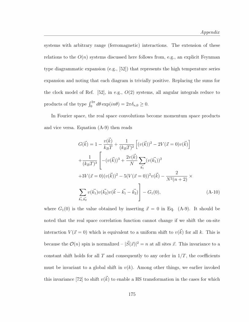
Appendix
systems with arbitrary range (ferromagnetic) interactions. The extension of these
relations to the O(n) systems discussed here follows from, e.g., an explicit Feynman
type diagrammatic expansion (e.g., [52]) that represents the high temperature series
expansion and noting that each diagram is trivially positive. Replacing the sums for
the clock model of Ref. [52], in e.g., O(2) systems, all angular integrals reduce to
products of the type∫ 2π
0dθ exp(inθ) = 2πδn,0 ≥ 0.
In Fourier space, the real space convolutions become momentum space products
and vice versa. Equation (A-9) then reads
G(~k) = 1− v(~k)
kBT+
1
(kBT )2
[
(v(~k))2 − 2V (~x = 0)v(~k)]
+1
(kBT )3
−(v(~k))3 +2v(~k)
N
∑
~k1
(v(~k1))2
+3V (~x = 0)(v(~k))2 − 5(V (~x = 0))2v(~k)− 2
N2(n+ 2)×
∑
~k1, ~k2
v(~k1)v(~k2)v(~k − ~k1 − ~k2)
−G1(0), (A-10)
where G1(0) is the value obtained by inserting ~x = 0 in Eq. (A-9). It should be
noted that the real space correlation function cannot change if we shift the on-site
interaction V (~x = 0) which is equivalent to a uniform shift to v(~k) for all k. This is
because the O(n) spin is normalized – |~S(~x)|2 = n at all sites ~x. This invariance to a
constant shift holds for all T and consequently to any order in 1/T , the coefficients
must be invariant to a global shift in v(k). Among other things, we earlier invoked
this invariance [72] to shift v(~k) to enable a HS transformation in the cases for which
175

Appendix
initially v(~k) > 0 for some values of ~k. We can, of course, invoke this invariance here
also to obtain the above high temperature series expansion with a well-defined HS
dual. The final results, as we re-iterated above are invariant under this shift as is
also manifest in our series expansion in powers of 1/T . Although obvious, we note
that the expansion in Eq. (A-10) is performed in powers of 1/T involving v(k) for
real vectors ~k. In examining the correlation lengths via contour integration in the
complex k plane, the corresponding v(k) may be extended for complex k.
We see from the expansion in Eq. (A-10) that already to O(1/T ), it is also
clear that the lengthscales of the system (which are determined by the poles of the
Fourier space correlation function) are governed by the poles of v(~k) in the complex
~k space. Thus, if, e.g., v(~k) = 1/(k2 + λ−2), the correlation length tends to λ at high
temperature. It therefore must diverge for a system with no screening.
In cases where the correlation function is known from some experimental technique
or otherwise, the series expansion for the correlation function can be inverted to arbi-
trary order to obtain the pairwise interactions. To O(1/T 2), for non-zero separation
~x, the potential function is given by,
V (~x) = −kBT[
G(~x)−∑
~z
′G(~z)G(~x− ~z)
+∑
~y,~z
′G(~y)G(~z)G(~x− ~y − ~z)
+2G(~x)∑
~z
′G(~z)G(−~z)− 2 (G(~x))3
n+ 2
]
. (A-11)
The prime indicates that the sum excludes terms containing G(0). As is evident from
176
Appendix
our earlier results and discussion, in Eq. (A-11), each correlation function G(~x) is of
order (1/T ).
We reiterate that, as in our discussion in Sec. 3.6, our results for lattice O(n) spin
models match with the leading order behavior at high temperature obtained from
several standard approximate theories based on Mayer’s cluster expansion derived for
liquid systems, e.g., Born-Green theory [148] and OZ theory with the Percus-Yevick
approximation [149] or MSA [93]. As implicit above, our 1/T expansion can indeed
be extended to systems in which the liquid and the gas phase are not separated by a
phase transition, e.g., for pressures larger than the pressure at the liquid-vapor criti-
cal point. As further noted in Sec. 3.6, various approximations also suggest that at
high temperatures, the correlation length may match the length scale characterizing
the interaction potential and, in particular, will diverge in systems having long range
interactions (as we have established).
177

Appendix
B Relation between the generalized Debye lengths
and divergence of the high temperature corre-
lation lengths
An intuitive approximate approach for the understanding of the rigorous yet seem-
ingly paradoxical result that we report in this work – that of the divergence of the
correlation lengths in the high temperature limit of systems with long range inter-
actions – is afforded by the OZ framework. Specifically, in the language of OZ ap-
proximations, the “total” high temperature correlation function is the same as the
“direct” correlation function [see, e.g., Ref. [77] (Sec. 2.6) for the definition of the
“direct” OZ correlation functions] and behaves as
G(~x) ∼ −βV (~x) (B-12)
for ~x 6= 0. Thus, if the potential is screened beyond a distance λ, the correlation
length approaches λ at high temperature. That is, if we have an effective interaction
resulting, e.g., from higher order effects in 1/T , such as that leading to the Debye
screening length (λD) in Coulomb systems [and generalizations introduced earlier in
Eq. (3.18)], then at high temperature, the correlation length
ξ −−−→T→∞
λD. (B-13)
This is a particular case of Eq. (3.15).
178

Appendix
To O(1/T 2), Eq. (A-10) is identical to Eq. (3.10). The poles of G in the complex
k plane can, of course, be computed by finding those of Eq. (3.10) or considering
directly those of Eq. (A-10): both give rise to the same answer as they must.
C Transfer Matrix in the one-dimensional system
with Ising spins
Thus far, we focused primarily on high dimensional continuous (large-n) spin sys-
tems. For completeness, we review and illustrate how some similar conclusions can
be drawn for one-dimensional Ising systems with finite ranged interactions and briefly
discuss trivial generalizations. In particular, we show how the sum of the number of
modulation and number of correlation lengths does not change as the temperature is
varied. In Sec. 4.3.3, we illustrated how this arises for general large-n systems.
For interactions of range R in a one-dimensional Ising spin chain, the transfer
matrix, T is of dimensionM = O(2R). The correlation function for large system size,
takes the form
G(x) =2R−1∑
k=1
Ak
(
λkλ0
)x
, (C-14)
where λis are the eigenvalues of the transfer matrix. Since the characteristic equation
has real non-negative coefficients, from Perron-Frobenius theorem, λ0 is real, positive
and is non-degenerate. The secular equation, det(T − λI) = 0 is a polynomial in λ
with real coefficients. Thus, two possibilities need to be examined: real roots, and,
179

Appendix
complex conjugate pairs of roots. Real eigenvalues λp give terms with correlation
length,
ξ = ln
(
λ0|λp|
)
. (C-15)
Complex conjugate eigenvalues, λq and λ∗q correspond to the same correlation length
and modulation length, given by,
ξ = ln
(
λ0|λq|
)
, (C-16)
LD =2π
tan−1(
Im{λq}Re{λq}
) . (C-17)
Thus, the total number of correlation and modulation lengths is the order of the
polynomial in λ in the secular equation, or simply the dimension of the transfer
matrix – O(2R). Similar to our conclusions for the high dimensional continuous spin
systems, this number does not vary with temperature. For q state Potts type spins,
replicating the above arguments mutatis mutandis, we find that the total number of
correlation and modulation lengths is O(qR). Similarly, for such a system placed on
a d-dimensional slab of finite extent in, at least, (d− 1) directions along which it has
a length of order O(l) > R, there will be O(qld−1
) transfer matrix eigenvalues and
thus an identical number for the sum of the number of modulation lengths with the
number of correlation lengths.
The eigenvalues change from being complex below certain crossover temperatures
to being purely real above. These temperatures form the “disorder line”.
180

Appendix
D Detailed expressions for δLD for different orders
p(≥ 3) at which the interaction kernel has its
first non-vanishing derivative
If the lowest order (larger than p = 2) non-vanishing derivative of v(k) at the minimiz-
ing wavenumber k0 (see Eq. (4.31)) is of order p = 3 (the most common case) then,
in the large-n limit, the change in the modulation length at temperatures T > Tc
(µ(T ) = µmin + δµ)about its value at T = Tc of Eq. (4.41) is given by
δLD = −2π
k20
v(3)(k0)δµ
3(v(2)(k0))2. (D-18)
We employ Eq. (D-18) in our analysis in Sec. 4.4. If the lowest order derivatives are
of order p = 4 or 5 then,
δLD =2π
k20
v(5)(k0)(δµ)2
30(v(2)(k0))3. (D-19)
Similarly, for p = 6 or 7,
δLD = −2π
k20
v(7)(k0)(δµ)3
630(v(2)(k0))4, (D-20)
and so on.
E µ(T ) for the screened Coulomb ferromagnet
We now briefly provide an explicit expression for the relation between the large-n
Lagrange multiplier µ and the temperature T for the screened Coulomb ferromagnet.
181

Appendix
In three dimensions, with Λ as an ultra-violet cutoff, at high temperatures [T > T ∗],
we get to the following implicit equation for µ(T ) in the case of the screened Coulomb
ferromagnet of Eq. (4.64),
1
T=
Λ
2π2+
√2
4π2w
×(λ2µ− µ2 + µw − 2Q
√
λ2 + µ+ wtan−1(
Λ√2
√
λ2 + µ+ w)
−λ2µ− µ2 + µw + 2Q√
λ2 + µ− wtan−1(
Λ√2
√
λ2 + µ− w))
. (E-21)
In Eq. (E-21), we employed the shorthand w ≡√
(µ− λ2)2 − 4Q. The parameter
w vanishes at the crossover temperature T ∗ at which a divergent modulation length
makes an appearance, w(T = T ∗) = 0. At low temperatures, T < T ∗, w becomes
imaginary and an analytical crossover occurs to another real functional form.
F Proof that µ(T ) is an analytic function of T
In this appendix, we illustrate that in the large-n limit, the thermodynamic functions
are analytic for all temperatures T > Tc, including the discussed cross-over tempera-
ture T = T ∗ (hence justifying the use of the term ”cross-over”) of, e.g, the Coulomb
frustrated ferromagnet of Eqs. (2.1, 4.64).
From Eq. (4.20), using,
µ > µmin = −min v(k), (F-22)
182

Appendix
it is clear that µ(T ) is a continuous function of T . Differentiating,
dµ
d(kBT )=
[
(kBT )2
∫
ddk
(v(k) + µ)2
]−1
, (F-23)
and,
d2µ
d(kBT )2= − 2
kBT
dµ
d(kBT )+
2(kBT )2
(
dµ
d(kBT )
)3 ∫ddk
(v(k) + µ)3(F-24)
with the integrations performed over the first Brillouin zone on the lattice (or up to
some ultra-violet cutoff Λ in the continuum). The first two derivatives are thus always
finite so long as the integration range is finite. All higher order derivatives are sum of
terms which are products of lower order derivatives, (kBT )a and
∫
ddk(v(k)+µ)b
, where a
and b are integers, with b > 0. Thus, for finite integration range, µ(T ) is an analytic
function of T . In the large-n limit, the internal energy per site, U/N = [kBT−µ(T )]/2.
Our result concerning the analyticity of µ(T ) implies that the internal energy is
analytic and thus all of its derivatives and all other thermodynamic potentials.
G Fermi systems
In this appendix, we discuss several examples of non-interacting fermionic systems
where we observe a correlation or modulation length exponent. We will, in what
follows, ignore spin degrees of freedom which lead to simple degeneracy factors for
the systems that we analyze. In non-interacting Fermi systems, the mode occupancies
183

Appendix
are given by the Fermi function. That is,
〈n(~k)〉 = 〈c†(~k)c(~k)〉 = 1
eβ(ǫ(~k)−µ) + 1, (G-25)
where c(~k) and c†(~k) are the annihilation and creation operators at momentum ~k and
β = 1/(kBT ) with T the temperature. The correlation function associated with the
amplitude for hopping from the origin to lattice site ~x is given by
G(~x) = 〈C†(0)C(~x)〉 =∑
~k
〈n(~k)〉e−i~k·~x. (G-26)
Thus far, in most explicit examples that we considered we discussed scaling with
respect to a crossover temperature. In what follows, we will, on several occasions,
further consider the scaling of correlation and modulation lengths with the chemical
potential µ. We will use the letter υ to represent exponents corresponding to scaling
with respect to µ and continue to use ν to represent scaling with respect to the
temperature T .
The existence of modulated electronic phases is well known.[32, 150–164] In par-
ticular, the Fermi wave-vector dominated response of diverse modulated systems as
evident in Lindhard functions, particular features of charge and spin density waves
dominated by Fermi surface considerations in quasi- one dimensional and other sys-
tems have long been discussed and have numerous experimental realizations in diverse
compounds.[163, 164] The exponents that we derived in this work appear for all elec-
tronic and other systems in which a crossover occurs in the form of the modulations
seen in charge, spin, or other degrees of freedom. Our derived results concerning scal-
184

Appendix
ing apply to general interacting systems. To highlight essential physics as it pertains
to the change of modulations in systems of practical importance, we briefly review
and further discuss free electron systems.
G.1 Zero temperature length scales – Scaling as a function
of the chemical potential µ
We first consider a non-interacting fermionic system with a dispersion ǫ(~k). At zero
temperature, the number of particles occupying the Fourier mode ~k is given by
〈n(~k)〉 =
1 for ǫ(~k) < µ
0 for ǫ(~k) > µ.
(G-27)
All correlation functions as all other zero temperature thermodynamic properties, are
determined by the Fermi surface geometry. We now consider the correlation function
of Eq. (G-26). This correlation function will generally exhibit both correlation and
modulation lengths. To obtain the modulation lengths along a chosen direction (the
direction of the displacement ~x), a ray along that direction may be drawn. The
intercept of this ray with the Fermi surface provides the pertinent modulation wave-
vectors. As we vary µ we alter the density, ρ via
ρ = gs
∫
ǫ(~k)<µ
ddk
(2π)d, (G-28)
gs being the spin degeneracy (gs = 2 for non-interacting spin-half particles such as
electrons). As the Fermi surface topology is varied, the following effects may be
185

Appendix
observed.
1. If two branches of the Fermi surface touch each other at µ = µ0 and are disjoint
for all other values of µ, then a smooth crossover will appear from one set
of modulation lengths to another with |LD − LD0| ∝ |µ − µ0| on both sides
of the crossover. This crossover will be associated with an exponent υL =
1 characterizing the scaling of the modulation lengths with deviations in the
chemical potential. An example where a crossover of this kind is realized is the
ǫg = 0 case of the schematic shown in Fig. 7.14 in which the crossover occurs
at µ = µ0. Other examples of this occur at half filling of the square lattice
Figure 7.14: Transition from a metal to a band insulator. This figure is for illustration
only.
tight binding model and at three-quarters filling of the triangular lattice tight
binding model. These will be discussed later.
186

Appendix
2. If on the other hand, one branch of the Fermi surface vanishes as we go past
µ = µ0, the crossover is not so smooth and we get some rational fraction υL
(usually υL = 1/2) as the crossover exponent: |LD − LD0| ∝ |µ− µ0|υL , on one
side of the crossover. An example of this is shown in Fig. 7.15. Here,
|LD − LD0| =L2D0
2π
√
2|µ− µ0||ǫ′′(2π/LD0)|
, (G-29)
where LD0 is the modulation length at the point where the µ = µ0 line touches
the ǫ(k) curve, such that ǫ′(2π/LD0) = 0 The hopping correlation function takes
the form,
G(x) =(ax)d/2Jd/2(ax)
(2π)d/2xd− (bx)d/2Jd/2(bx)
(2π)d/2xd
+(cx)d/2Jd/2(cx)
(2π)d/2xd, (G-30)
where µ′0 < µ < µ0 and a, b and c in Eq. (G-30) (corresponding to modulation
lengths of 2π/a, 2π/b and 2π/c) are the values of k for which ǫ(k) = µ (as
shown in Fig. 7.15).
At arbitrarily small but finite temperatures, the correlation function exhibits mod-
ulations of all possible wavelengths. The prefactor multiplying a term with spatial
modulations at wave-vector ~k is the exponential of (−|ǫ(~k) − µ|). An illustrative
example is provided in Fig. 7.16. Apart from the dominant zero temperature modu-
lations, associated with the wave-vector k2 in Fig. 7.16, at finite temperature, there
are additional contributions from wave-vectors for which |ǫ(k) − µ| is small relative
187

Appendix
to kBT . Near k2, we can assume ǫ(k) is linear such that ǫ(k) ≈ µ + (k − k2)ǫ′(k2).
Similarly, near k1, ǫ(k) − µ ≈ −∆ − (k − k1)2ǫ′′(k1)/2, where ∆ = µ − µ0 (see Fig.
7.16). For large β, both these contributions are highly localized around k2 and k1 re-
spectively making the above approximations very good and the Fourier transforming
integrals easy to evaluate (〈n(~k)〉 taking exponential and Gaussian forms). We have,
G(x) =(k2x)
d/2Jd/2(k2x)
(2π)d/2xd− 2(k2x)
d/2Jd/2−1(k2x)
(2π)d/2βǫ′(k2)xd−1
+e−β∆(k1x)
d/2Jd/2−1(k1x)
(2π)d−12
√
βǫ′′(k1)xd−1, (G-31)
where β → ∞ and ∆ → 0, such that β∆ → ∞.
(a)
a b c kx
ky
(b) (c)
Figure 7.15: Example of a Fermi system where the modulation length exponent is 1/2.
The gray region shows the filled states. When µ > µ0, modulations cor-
responding to wave-vectors k = a and k = b cease to exist and we get an
exponent of 1/2 at this crossover. Similarly, when µ < µ′0, modulations
corresponding to wave-vectors k = b and k = c die down.
188

Appendix
Figure 7.16: The same Fermi system as in Fig. 7.15, but now with a chemical potential
µ = µ0 +∆, slightly higher than µ0. The temperature is small but finite.
Next, we will discuss scaling of the modulation length in with the chemical po-
tential, µ in the familiar tight binding models on the square and triangular lattices
at zero temperature.
Tight binding model on the square lattice
We consider a two-dimensional tight binding model of the square lattice. The disper-
sion in this model is given by
ǫ(~k) = −2t (cos kx + cos ky) . (G-32)
The constant energy contours corresponding to Eq. (G-32) are drawn in Fig. 7.17.
As is clear from Fig. 7.17, there are certain directions (e.g., along the X-axis) along
which there is no ~k for ǫ(~k) > 0. If we consider the same system at zero temperature,
189

Appendix
-3 -2 -1 0 1 2 3k
x
-3
-2
-1
0
1
2
3
k y
Figure 7.17: Constant energy contours for two-dimensional tight binding model on the
square lattice in Eq. (G-32). The red square corresponds to the particle hole
symmetric contour where ǫ(~k) = 0. The contours inside it are for negative
ǫ(~k) and those outside are for positive ǫ(~k).
the following three crossovers are observed.
(i) Half filling: The chemical potential µ is zero at the half filling state. The Fermi
surface is given by ±kx ± ky = π. For small µ, we have,
±kx ± ky = π +µ
2t sin kx, (G-33)
thus giving us an uninteresting modulation exponent, υL = 1.
(ii) Empty band: When µ = −4t, none of the states are occupied. As we increase µ
by a tiny amount δµ above this value, we observe a non-zero modulation wave-vector,
190

Appendix
k =√
δµ/t, thus showing a modulation exponent υL = 1/2.
(iii) Full inert bands: When µ = +4t, all the states are occupied. As we lower µ
by a tiny amount δµ below this value, we observe a difference δk of the modulation
vector from ±exπ± eyπ. We have, δk =√
δµ/t, thus showing a modulation exponent
υL = 1/2 again.
Tight binding model on the triangular lattice
The analysis of the triangular lattice within the tight binding approximation, is very
similar to the square lattice discussed above. The dispersion ǫ(~k) is given by
ǫ(k) = −2t cos kx − 4t coskx2cos
ky√3
2. (G-34)
We have exponents similar to the square lattice.
(i) Three-quarters filling: The chemical potential µ = 2t corresponds to the three-
quarters filling state. If we concentrate on the {kx = π, ky : −π/√3 → π/
√3}
segment (same phenomenon is present at all the other segments of the quarter filling
Fermi surface), we get,
δkx ∼ δµ
2 cos(
ky√3
2
) , (G-35)
where kx = π+δkx is obtained when µ = 2t+δµ. This leads to a modulation exponent
of υL = 1. The Fermi surfaces for chemical potentials µ close to three-quarters filling
are schematically shown in Fig. 7.18.
(ii) Empty band: When µ = −6t, none of the states is occupied. As we increase µ by
191

Appendix
a tiny amount δµ above this value, we observe a non-zero modulation wave-vector,
k =√
2δµ/3, thus showing a modulation exponent υL = 1/2.
(iii) Full inert bands: When µ = 3t, all of the states are occupied and close to this
value the Fermi surface is composed of six small circles around ~k = x cos(nπ/3) +
y sin(nπ/3), n = {0, 1, 2, 3, 4, 5}. If µ = 3t− δµ, we get, | ~δk| = 2√
δµ/3, again giving
us a modulation length exponent, υL = 1/2.
Metal-Insulator transition
We discuss here the metal to band insulator transition at zero temperature. In a
non-interacting system, this occurs when the Fermi energy is changed such that all
occupied bands become completely full, as shown in Fig. 7.14. In the insulator, the
Fermi energy lies in between two bands and thus the filled states are separated from
the empty states by a finite energy gap. As the Fermi energy is tuned, the Fermi
energy might touch one of the bands thereby rendering the system metallic. Close to
this transition, the energy is quadratic in the momentum k, i.e., |k| ∝ |δµ|1/2. This
implies that,
|δk| ∝ |δµ|1/2. (G-36)
Following the scaling convention in Eq. (5.7), we adduce a similar exponent
υL = 1/2 (G-37)
192

Appendix
-6 -4 -2 0 2 4 6
-6
-4
-2
0
2
4
6
(a) µ = 1.8
-6 -4 -2 0 2 4 6
-6
-4
-2
0
2
4
6
(b) µ = 2.2
-6 -4 -2 0 2 4 6
-6
-4
-2
0
2
4
6
(c) µ = 2.2(blue), µ =
2(green) and µ = 1.8(red)
Figure 7.18: Fermi surface for a triangular lattice with tight binding. The dashed lines are
the Brillouin zone boundaries. This demonstrates a smooth crossover from
one set of Fermi surface branches to another as µ is changed across µ = 2.
The points where the crossovers take place are (0,±2π/√3), (±π,±π/
√3).
The modulation length exponent for this crossover is υL = 1.
that governs the scaling of the modulation lengths with the shift δµ of the chemical
potential (instead of temperature variations).
193

Appendix
Dirac systems
The low energy physics of graphene and Dirac systems is characterized by the exis-
tence of Dirac points in momentum space where the density of states vanishes and
the energy, ǫ(k) is proportional to the momentum k for small k. When we invoke and
repeat our earlier analysis to these systems, we discern a trivial exponent
|δk| ∝ |δµ|
=⇒ υDirac = 1. (G-38)
This exponent may be contrasted with that derived from Eq. (G-37).
Topological Insulators – Multiple length scale exponents as a function of
the chemical potential µ
The quintessential low energy physics of three-dimensional topological insulators can
be gleaned from the following effective Hamiltonian[165] in momentum space,
H(~k) = ǫ0(~k)I4×4 +
M(~k) A1kz 0 A2k−
A1kz −M(~k) A2k− 0
0 A2k+ M(~k) −A1kz
A2k+ 0 −A1kz −M(~k)
(G-39)
where ǫ0(~k) = C + D1k2z + D2k
2⊥, M(~k) = M − B1k
2z − B2k
2⊥ , with k± = kx + iky,
k⊥ =√
k2x + k2y and A1, A2, B1, B2, C, D1 and D2 constants for a given system. The
194

Appendix
0 0.02 0.04 0.06 0.08 0.1k⊥ (in 1/Å)
-0.4
-0.2
0
0.2
0.4
0.6
ε (in
eV
)
(a)
0 0.02 0.04 0.06 0.08 0.1k
z (in 1/Å)
-0.4
-0.2
0
0.2
0.4
ε (in
eV
)
(b)
ky
kx
εsurf
(kx,k
y)
(c)
Figure 7.19: Energy levels of Bi2Se3 topological insulator.
7.19(a): ǫ(~k) versus k⊥ at kz = 0; 7.19(b): ǫ(~k) versus kz at k⊥ = 0; 7.19(c):
ǫsurf (kx, ky) versus ~k⊥ ≡ (kx, ky).
energy bands are given by
ǫ(~k) = ǫ0(~k)±√
M(~k)2 + A1k2z + A2k2⊥. (G-40)
These bands are plotted in Figs. 7.19(a) and 7.19(b). The finite gap between the two
bands leads to an exponentially damped hopping amplitude, characterized by a finite
correlation length when the Fermi energy lies within this gap. These energy bands
195

Appendix
disperse quadratically for small k thus yielding
|δk| ∝√
|δµ|
=⇒ υbulk = 1/2 (G-41)
whenever the correlation length diverges and a insulator to metal transition takes
place in the bulk, thus allowing long range hopping. The same exponent is also ex-
pected whenever the modulation length becomes constant as µ crosses some threshold
value.
The effective Hamiltonian for the surface states is given by
Hsurf =
0 A2k−
A2k+ 0
, (G-42)
leading trivially to surface energies
ǫsurf (kx, ky) = ±A2k⊥. (G-43)
Similar to the Dirac points in graphene (see Fig. 7.19(c)), we trivially find an exponent
of
υsurf = 1. (G-44)
An example of a zero temperature Fermi system in which υL is not half or
one
Very large (or divergent) effective electronic masses meff can be found in heavy
fermion systems (and at putative quantum critical points).[166, 167] If the electronic
196

Appendix
dispersion ǫ(~k) has a minimum at ~k0 then a Taylor expansion about that minimum
trivially reads
ǫ(~k) = ǫ(~k0) +~2
2
∑
ij
(
m−1eff
)
ij(ki − k0i)(kj − k0j) +
∑
ijl
Aijl(ki − k0i)(kj − k0j)(kl − k0l) + . . . . (G-45)
When present, parity relative to ~k0 or other considerations may limit this expansion
to contain only even terms. As an example, we consider the dispersion
ǫ(k) = c1 − c2(k2 − k20)
4, (G-46)
where c2 > 0. The hopping correlation function of such a system has a term which
exhibits modulations at wave-vector k = k0 at µ = µ∗ = c1. At higher values of the
chemical potential, such a term ceases to exist. At lower values (µ = µ∗ − δµ), this
term breaks up into two terms whose modulation wave-vectors are different from k0
by,
k − k0 ∼ ± δµ1/4
2k0c1/42
,
=⇒ υL = 1/4. (G-47)
G.2 Finite temperature length scales – Scaling as a function
of temperature
At finite temperatures, apart from the modulation lengths, there generally is a set
of characteristic correlation lengths. From Eq. (G-26), these are obtained by finding
197
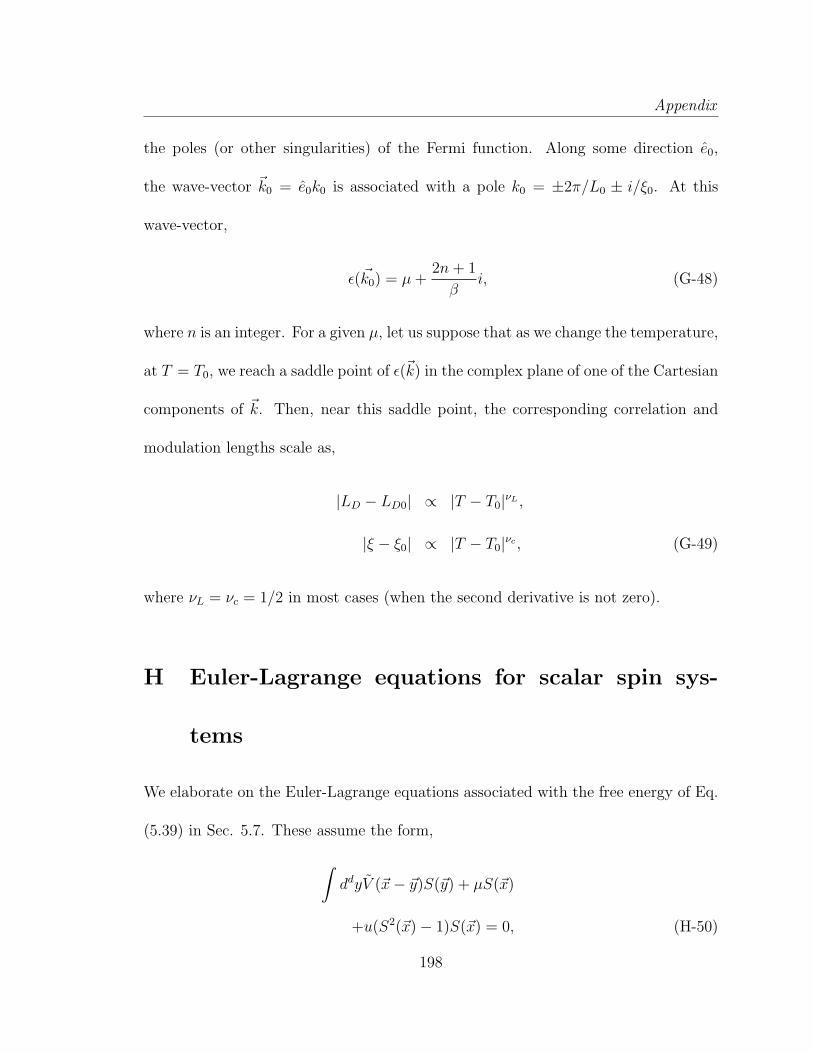
Appendix
the poles (or other singularities) of the Fermi function. Along some direction e0,
the wave-vector ~k0 = e0k0 is associated with a pole k0 = ±2π/L0 ± i/ξ0. At this
wave-vector,
ǫ(~k0) = µ+2n+ 1
βi, (G-48)
where n is an integer. For a given µ, let us suppose that as we change the temperature,
at T = T0, we reach a saddle point of ǫ(~k) in the complex plane of one of the Cartesian
components of ~k. Then, near this saddle point, the corresponding correlation and
modulation lengths scale as,
|LD − LD0| ∝ |T − T0|νL ,
|ξ − ξ0| ∝ |T − T0|νc , (G-49)
where νL = νc = 1/2 in most cases (when the second derivative is not zero).
H Euler-Lagrange equations for scalar spin sys-
tems
We elaborate on the Euler-Lagrange equations associated with the free energy of Eq.
(5.39) in Sec. 5.7. These assume the form,
∫
ddyV (~x− ~y)S(~y) + µS(~x)
+u(S2(~x)− 1)S(~x) = 0, (H-50)
198

Appendix
where V (~x) = [V (~x)+V (−~x)]/2. For example, if we consider the finite ranged system
for which,
∫
ddyV (~x− ~y)S(~y) = a∇2S(~x)
+ b∇4S(~x) + . . . , (H-51)
then, we have,
a∇2S(~x) + b∇4S(~x) + . . .+ µS(~x)
+ u(S2(~x)− 1)S(~x) = 0. (H-52)
For lattice systems, the Euler Lagrange equation (H-50) reads
∑
~y
V (~x− ~y)S(~y) + µS(~x)
+ u(S2(~x)− 1)S(~x) = 0. (H-53)
In general, it may be convenient to express the linear terms in the above equation in
terms of the lattice Laplacian ∆. We write
D(∆)S(~x) ≡∑
~y
V (~x− ~y)S(~y) + µS(~x), (H-54)
D being some operator which is a function of the lattice Laplacian ∆. The real-space
lattice Laplacian ∆, given by the Fourier transform of Eq. (2.7), acts on a general
field f as
∆f(~x) ≡ −d∑
i=1
[f(~x+ ei) + f(~x− ei)− 2f(~x)]. (H-55)
199

Appendix
Here, {ei} denote unit vectors along the Cartesian directions. (In the continuum
limit, ∆ can be replaced by −∇2.) The Euler-Lagrange equation then, takes the
form,
D(∆)S(~x) + u(S2(~x)− 1)S(~x) = 0. (H-56)
Equation H-51 corresponds, on the lattice, to
∑
~y
V (~x− ~y)S(~y) =
−a∆S(~x) + b∆2S(~x) + . . . . (H-57)
The Euler Lagrange equation for this finite ranged system reads
−a∆S(~x) + b∆2S(~x) + . . .+ µS(~x)
+ u(S2(~x)− 1)S(~x) = 0. (H-58)
200

Bibliography
[1] A. Mesaros, K. Fujita, H. Eisaki, S. Uchida, J. C. Davis, S. Sachdev, J. Zaanen,
M. J. Lawler, and Eun-Ah Kim. Topological defects coupling smectic mod-
ulations to intraunit-cell nematicity in cuprates. Science, 333(6041):426–430,
2011.
[2] Michael Seul and David Andelman. Domain shapes and patterns: The phe-
nomenology of modulated phases. Science, 267(5197):476–483, 1995.
[3] Per Bak and J. von Boehm. Ising model with solitons, phasons, and “the devil’s
staircase”. Phys. Rev. B, 21:5297–5308, Jun 1980.
[4] A. Gendiar and T. Nishino. Phase diagram of the three-dimensional axial next-
nearest-neighbor Ising model. Phys. Rev. B, 71:024404, Jan 2005.
[5] J. C. Sprott. Simple chaotic systems and circuits. American Journal of Physics,
68(8):758–763, 2000.
[6] Peter Ronhovde and Zohar Nussinov. Multiresolution community detection for
201

Bibliography
megascale networks by information-based replica correlations. Phys. Rev. E,
80(1):016109, Jul 2009.
[7] J. A. Moriarty and M. Widom. First-principles interatomic potentials for
transition-metal alumnides: Theory and trends across the 3d series. Phys.
Rev. B, 56(13), Oct 1997.
[8] J. Stadler, R. Mikulla, and H. R. Trebin. IMD: A software package for molec-
ular dynamics studies on parallel computers. International Journal of Modern
Physics C, 8(5):1131–1140, Jun 1997.
[9] Walter Kob and Hans C. Andersen. Testing mode-coupling theory for a su-
percooled binary Lennard-Jones mixture I: The van Hove correlation function.
Phys. Rev. E, 51(5):4626–4641, May 1995.
[10] S.K. Ma. Modern Theory Of Critical Phenomena. Advanced Book Classics.
Perseus, 2000.
[11] Kenneth G. Wilson. Renormalization group and critical phenomena. I. renor-
malization group and the Kadanoff scaling picture. Phys. Rev. B, 4:3174–3183,
Nov 1971.
[12] M E Fisher. The theory of equilibrium critical phenomena. Reports on Progress
in Physics, 30(2):615, 1967.
202

Bibliography
[13] The approach of defining an order parameter does not work in many situations,
e.g., gauge theories, classicalXY models, one-dimensional quantum spin chains,
etc. .
[14] Ernst Ising. Beitrag zur theorie des ferromagnetismus. Zeitschrift fur Physik A
Hadrons and Nuclei, 31:253–258, 1925.
[15] T. Dauxois, S. Ruffo, E. Arimondo, and M. Wilkens. Dynamics and Thermo-
dynamics of Systems With Long Range Interactions. Lecture Notes in Physics.
Springer, Berlin Heidelberg, 2010.
[16] Alessandro Giuliani, Joel L. Lebowitz, and Elliott H. Lieb. Striped phases in
two-dimensional dipole systems. Phys. Rev. B, 76:184426, Nov 2007.
[17] Alessandro Giuliani, Joel L. Lebowitz, and Elliott H. Lieb. Ising models with
long-range antiferromagnetic and short-range ferromagnetic interactions. Phys.
Rev. B, 74:064420, Aug 2006.
[18] Alessandro Vindigni, Niculin Saratz, Oliver Portmann, Danilo Pescia, and Paolo
Politi. Stripe width and nonlocal domain walls in the two-dimensional dipolar
frustrated Ising ferromagnet. Phys. Rev. B, 77:092414, Mar 2008.
[19] C. Ortix, J. Lorenzana, and C. Di Castro. Frustrated phase separation in two-
dimensional charged systems. Phys. Rev. B, 73:245117, Jun 2006.
203

Bibliography
[20] Istvan Daruka and Zsolt Gulacsi. Correlation transitions in the Ising chain
with competing short-range and long-range mirror interactions. Phys. Rev. E,
58:5403–5409, Nov 1998.
[21] Daniel G. Barci and Daniel A. Stariolo. Orientational order in two dimensions
from competing interactions at different scales. Phys. Rev. B, 79:075437, Feb
2009.
[22] Michael Fogler. Stripe and bubble phases in quantum hall systems. In
C. Berthier, L. Levy, and G. Martinez, editors, High Magnetic Fields, volume
595 of Lecture Notes in Physics, pages 98–138. Springer, Berlin Heidelberg,
2002.
[23] Hyung-June Woo, Carlo Carraro, and David Chandler. Quantitative molecular
interpretation of mesoscopic correlations in bicontinuous microemulsions. Phys.
Rev. E, 52:6497–6507, Dec 1995.
[24] Frank H. Stillinger. Variational model for micelle structure. The Journal of
Chemical Physics, 78(7):4654–4661, 1983.
[25] Ludwik Leibler. Theory of microphase separation in block copolymers. Macro-
molecules, 13(6):1602–1617, 1980.
[26] Takao Ohta and Kyozi Kawasaki. Equilibrium morphology of block copolymer
melts. Macromolecules, 19(10):2621–2632, 1986.
204

Bibliography
[27] H. Kleinert. Gauge fields in condensed matter. Number v. 2 in Gauge Fields in
Condensed Matter. World Scientific, 1989.
[28] Pierre-Henri Chavanis. Statistical mechanics of two-dimensional vortices and
stellar systems. In Thierry Dauxois, Stefano Ruffo, Ennio Arimondo, and Mar-
tin Wilkens, editors, Dynamics and Thermodynamics of Systems with Long-
Range Interactions, volume 602 of Lecture Notes in Physics, pages 208–289.
Springer Berlin Heidelberg, 2002.
[29] H. Kleinert. Gauge fields in condensed matter. Number v. 1 in Gauge Fields in
Condensed Matter. World Scientific, 1989.
[30] Yves Elskens. Kinetic theory for plasmas and wave-particle hamiltonian dynam-
ics. In Thierry Dauxois, Stefano Ruffo, Ennio Arimondo, and Martin Wilkens,
editors, Dynamics and Thermodynamics of Systems with Long-Range Interac-
tions, volume 602 of Lecture Notes in Physics, pages 437–447. Springer Berlin
Heidelberg, 2002.
[31] Y Elskens and D Escande. Microscopic dynamics of plasmas and chaos. Plasma
Physics and Controlled Fusion, 45(4):521, 2003.
[32] V.J. Emery and S.A. Kivelson. Frustrated electronic phase separation and high-
temperature superconductors. Physica C: Superconductivity, 209(4):597 – 621,
1993.
205

Bibliography
[33] L. Chayes, V.J. Emery, S.A. Kivelson, Z. Nussinov, and G. Tarjus. Avoided crit-
ical behavior in a uniformly frustrated system. Physica A: Statistical Mechanics
and its Applications, 225(1):129 – 153, 1996.
[34] Zohar Nussinov, Joseph Rudnick, Steven A. Kivelson, and L. N. Chayes.
Avoided critical behavior in O(n) systems. Phys. Rev. Lett., 83:472–475, Jul
1999.
[35] U. Low, V. J. Emery, K. Fabricius, and S. A. Kivelson. Study of an Ising
model with competing long- and short-range interactions. Phys. Rev. Lett.,
72(12):1918–1921, Mar 1994.
[36] E. W. Carlson, V. J. Emery, S. A. Kivelson, and D. Orgad. Concepts in high
temperature superconductivity. In K. H. Bennemann and John B. Ketterson,
editors, Superconductivity, chapter 21, pages 1225–1348. Springer Berlin Hei-
delberg, 2008. See also arXiv:cond-mat/0206217.
[37] V. B. Nascimento, Ang Li, Dilushan R. Jayasundara, Yi Xuan, Jared O’Neal,
Shuheng Pan, T. Y. Chien, Biao Hu, X. B. He, Guorong Li, A. S. Sefat, M. A.
McGuire, B. C. Sales, D. Mandrus, M. H. Pan, Jiandi Zhang, R. Jin, and E. W.
Plummer. Surface geometric and electronic structures of BaFe2As2(001). Phys.
Rev. Lett., 103:076104, Aug 2009.
[38] S-W. Cheong, G. Aeppli, T. E. Mason, H. Mook, S. M. Hayden, P. C. Can-
206

Bibliography
field, Z. Fisk, K. N. Clausen, and J. L. Martinez. Incommensurate magnetic
fluctuations in La2−xSrxCuO4. Phys. Rev. Lett., 67:1791–1794, Sep 1991.
[39] D. I. Golosov. Magnetic domain walls in single-phase and phase-separated
double-exchange systems. Phys. Rev. B, 67:064404, Feb 2003.
[40] Daniel Kivelson, Steven A. Kivelson, Xiaolin Zhao, Zohar Nussinov, and Gilles
Tarjus. A thermodynamic theory of supercooled liquids. Physica A: Statistical
and Theoretical Physics, 219(1-2):27 – 38, 1995.
[41] Jorg Schmalian and Peter G. Wolynes. Stripe glasses: Self-generated random-
ness in a uniformly frustrated system. Phys. Rev. Lett., 85:836–839, Jul 2000.
[42] M. Grousson, G. Tarjus, and P. Viot. Phase diagram of an Ising model
with long-range frustrating interactions: A theoretical analysis. Phys. Rev.
E, 62(6):7781–7792, Dec 2000.
[43] Zohar Nussinov. Avoided phase transitions and glassy dynamics in geomet-
rically frustrated systems and non-abelian theories. Phys. Rev. B, 69:014208,
2004.
[44] G Tarjus, S A Kivelson, Z Nussinov, and P Viot. The frustration-based ap-
proach of supercooled liquids and the glass transition: a review and critical
assessment. Journal of Physics: Condensed Matter, 17(50):R1143, 2005.
207

Bibliography
[45] B. V. Derjaguin and L. Landau, Acta Physiochim, URSS 14, 633 (1941); E.
J. Verwey and J. T. G. Overbeek Theory of Stability of Lyophobic Colloids
(Elsevier, Amsterdam, 1948).
[46] C. Reichhardt and C. J. Olson. Novel colloidal crystalline states on two-
dimensional periodic substrates. Phys. Rev. Lett., 88:248301, May 2002.
[47] Julien Barre, David Mukamel, and Stefano Ruffo. Ensemble inequivalence in
mean-field models of magnetism. In Thierry Dauxois, Stefano Ruffo, Ennio
Arimondo, and Martin Wilkens, editors, Dynamics and Thermodynamics of
Systems with Long-Range Interactions, volume 602 of Lecture Notes in Physics,
pages 45–67. Springer Berlin Heidelberg, 2002.
[48] Mark Ya. Azbel’. Long-range interaction and heterogeneity yield a different
kind of critical phenomenon. Phys. Rev. E, 68:050901, Nov 2003.
[49] S. Elitzur. Impossibility of spontaneously breaking local symmetries. Phys.
Rev. D, 12:3978–3982, Dec 1975.
[50] John B. Kogut. An introduction to lattice gauge theory and spin systems. Rev.
Mod. Phys., 51:659–713, Oct 1979.
[51] X.G. Wen. Quantum Field Theory of Many-Body Systems: From the Origin of
Sound to an Origin of Light and Electrons. Oxford graduate texts in mathe-
matics. Oxford University Press, 2007.
208

Bibliography
[52] G. Ortiz, E. Cobanera, and Z. Nussinov. Dualities and the phase diagram of
the p-clock model. Nuclear Physics B, 854(3):780 – 814, 2012.
[53] F. C. Frank. Supercooling of liquids. Proceedings of the Royal Society of London.
Series A. Mathematical and Physical Sciences, 215(1120):43–46, 1952.
[54] C. Dasgupta, A. V. Indrani, Sriram Ramaswamy, and M. K. Phani. Is there
a growing correlation length near the glass transition? Europhysics Letters,
15(3):307, 1991.
[55] Paul J. Steinhardt, David R. Nelson, and Marco Ronchetti. Bond-orientational
order in liquids and glasses. Phys. Rev. B, 28(2):784–805, 1983.
[56] G. Voronoi. Nouvelles applications des parametres continus a la theorie des
formes quadratiques. Deuxieme memoire. Recherches sur les parallelloedres
primitifs. Journal fur die reine und angewandte Mathematik, 134:198–287, 1908.
[57] J. Dana Honeycutt and Hans C. Andersen. Molecular dynamics study of melting
and freezing of small Lennard-Jones clusters. J. Phys. Chem., 91(19):4950–4963,
Sep 1987.
[58] Saurish Chakrabarty and Zohar Nussinov. High-temperature correlation func-
tions: Universality, extraction of exchange interactions, divergent correlation
lengths, and generalized Debye length scales. Phys. Rev. B, 84:064124, Aug
2011.
209

Bibliography
[59] Saurish Chakrabarty and Zohar Nussinov. Modulation and correlation lengths
in systems with competing interactions. Phys. Rev. B, 84:144402, Oct 2011.
[60] P. Ronhovde, S. Chakrabarty, D. Hu, M. Sahu, K. Sahu, K. Kelton, N. Mauro,
and Z. Nussinov. Detecting hidden spatial and spatio-temporal structures in
glasses and complex physical systems by multiresolution network clustering.
Euro. Phys. J. E, 34:1–24, 2011.
[61] P. Ronhovde, S. Chakrabarty, D. Hu, M. Sahu, K. K. Sahu, K. F. Kelton, N. A.
Mauro, and Z. Nussinov. Detection of hidden structures for arbitrary scales in
complex physical systems. Sci. Rep., 2:329, 2012.
[62] H. E. Stanley. Spherical model as a limit of infinite spin dimensionality. Phys.
Rev., 176(2):718–722, 1968.
[63] T. H. Berlin and M. Kac. The spherical model of a ferromagnet. Phys. Rev.,
86:821–835, Jun 1952.
[64] P. Debye and E. Huckel. Debye-Huckel theory of electrolytes. Phys. Z, 24:185,
1923.
[65] G.S. Rushbrooke and P.J. Wood. On the Curie points and high temperature sus-
ceptibilities of Heisenberg model ferromagnetics. Molecular Physics, 1(3):257–
283, 1958.
210

Bibliography
[66] H. E. Stanley and T. A. Kaplan. High-temperature expansions-the classical
Heisenberg model. Phys. Rev. Lett., 16:981–983, May 1966.
[67] K. Huang. Statistical mechanics. Wiley, 1987.
[68] J. Horbach, W. Kob, and K. Binder. Molecular dynamics simulation of the
dynamics of supercooled silica. Philosophical Magazine Part B, 77(2):297–303,
1998.
[69] R. L. Stratonovich. On a method of calculating quantum distribution functions.
Soviet Physics Doklady, 2:416, 1958.
[70] J. Hubbard. Calculation of partition functions. Phys. Rev. Lett., 3:77–78, Jul
1959.
[71] Y.M. Ivanchenko and A.A. Lisyansky. Physics of Critical Fluctuations. Grad-
uate Texts in Contemporary Physics. Springer-Verlag, 1995.
[72] The integrals in Eq.(3.3) converge if v(~k) is negative for all real ~k. This can
be achieved for all systems with finite range or screened interactions (with
an arbitrarily large screening length) when v(~k) is bounded from above. As
(~S(~x))2 = n for all ~x, the kernel v(~k) for all ~k can be trivially made negative
before performing the HS transformation by V (~x) → V (~x)+aδ~x,0 which merely
shifts the energy by an additive constant, H → H + anN/2, without changing
any averages.
211

Bibliography
[73] R. L. Henderson. A uniqueness theorem for fluid pair correlation functions.
Physics Letters A, 49(3):197 – 198, 1974.
[74] By “long range” we refer to systems for which V (~x) is not exactly zero
for arbitrary large ~x. In d spatial dimensions, for large distances, |V (~x)| ∝
exp(−|~x|/λ)/xa with 0 ≤ a ≤ d and λ is a “screening length” which can in
principle be arbitrarily large.
[75] By “charge neutrality”, we mean that∑
~y~S(~y) = 0 and, consequently, 〈~S(~x) ·
∑
~y~S(~y)〉 = 0 =⇒ ∑
~z G(~z) = 0.
[76] Z. Nussinov, C. D. Batista, B. Normand, and S. A. Trugman. High-dimensional
fractionalization and spinon deconfinement in pyrochlore antiferromagnets.
Phys. Rev. B, 75:094411, Mar 2007.
[77] N.H. March and P. Tosi. Atomic Dynamics in Liquids. Dover Books on Physics
and Chemistry. Dover, 1991.
[78] I. Dzyaloshinsky. A thermodynamic theory of weak ferromagnetism of anti-
ferromagnetics. Journal of Physics and Chemistry of Solids, 4(4):241 – 255,
1958.
[79] Toru Moriya. Anisotropic superexchange interaction and weak ferromagnetism.
Phys. Rev., 120:91–98, Oct 1960.
212

Bibliography
[80] Kliment I Kugel and D I Khomskii. The Jahn-Teller effect and magnetism:
transition metal compounds. Soviet Physics Uspekhi, 25(4):231, 1982.
[81] Zohar Nussinov and Eduardo Fradkin. Discrete sliding symmetries, dualities,
and self-dualities of quantum orbital compass models and p+ip superconducting
arrays. Phys. Rev. B, 71:195120, May 2005.
[82] Ran Budnik and Assa Auerbach. Low-energy singlets in the Heisenberg anti-
ferromagnet on the Kagome lattice. Phys. Rev. Lett., 93:187205, Oct 2004.
[83] Alexei Kitaev. Anyons in an exactly solved model and beyond. Annals of
Physics, 321(1):2 – 111, 2006.
[84] J. F. Sadoc and R. Mosseri. Geometrical Frustration. Cambridge University
Press, 1999.
[85] J. F. Sadoc and F. Mosseri. Amorphous Materials. American Institute of
Metallurgical Engineering New York, 1983.
[86] D. R. Nelson. Defects and Geometry in Condensed Matter Physics. Cambridge
University Press, 2002.
[87] Sadoc, J.F. Periodic networks of disclination lines : application to metal struc-
tures. J. Physique Lett., 44(17):707–715, 1983.
[88] Sadoc, J.F. and Charvolin, J. Frustration in bilayers and topologies of liquid
crystals of amphiphilic molecules. J. Phys. France, 47(4):683–691, 1986.
213

Bibliography
[89] David R. Nelson and Michael Widom. Symmetry, Landau theory and polytope
models of glass. Nuclear Physics B, 240(1):113 – 139, 1984.
[90] David R. Nelson. Order, frustration, and defects in liquids and glasses. Phys.
Rev. B, 28:5515–5535, Nov 1983.
[91] James P. Sethna. Frustration, curvature, and defect lines in metallic glasses
and the cholesteric blue phase. Phys. Rev. B, 31:6278–6297, May 1985.
[92] Subir Sachdev and David R. Nelson. Statistical mechanics of pentagonal and
icosahedral order in dense liquids. Phys. Rev. B, 32:1480–1502, Aug 1985.
[93] J. L. Lebowitz and J. K. Percus. Mean spherical model for lattice gases with
extended hard cores and continuum fluids. Phys. Rev., 144:251–258, Apr 1966.
[94] Here, we adhere to the prevalent practice of effectively setting β = 1 (with the
temperature dependence relegated solely to the prefactor r of Eq.(3.30)).
[95] Shang-keng Ma. Critical exponents above Tc to O( 1n). Phys. Rev. A, 7:2172–
2187, Jun 1973.
[96] Kenneth G. Wilson and Michael E. Fisher. Critical exponents in 3.99 dimen-
sions. Phys. Rev. Lett., 28:240–243, Jan 1972.
[97] C. B. Muratov. Theory of domain patterns in systems with long-range interac-
tions of Coulomb type. Phys. Rev. E, 66(6):066108, Dec 2002.
214

Bibliography
[98] Z. Nussinov, arXiv:cond-mat/0105253 (2001) – in particular, see footnote [20]
therein for the Ising ground states.
[99] John Stephenson. Ising model with antiferromagnetic next-nearest-neighbor
coupling: Spin correlations and disorder points. Phys. Rev. B, 1:4405–4409,
Jun 1970.
[100] John Stephenson. Range of order in antiferromagnets with next-nearest neigh-
bor coupling. Canadian Journal of Physics, 48(18):2118–2122, 1970.
[101] Nelson Alves Jr. and Carlos S. O. Yokoi. Spin pair correlation of the ANNNI
chain in a field. Brazilian Journal of Physics, 30:667 – 670, 12 2000.
[102] Walter Selke. The ANNNI model – theoretical analysis and experimental ap-
plication. Physics Reports, 170(4):213 – 264, 1988.
[103] S A Brazovskii. Phase transition of an isotropic system to a nonuniform state.
Sov Phys JETP, 41(1):85, 1975.
[104] Harry Westfahl, Jorg Schmalian, and Peter G. Wolynes. Self-generated ran-
domness, defect wandering, and viscous flow in stripe glasses. Phys. Rev. B,
64:174203, Oct 2001.
[105] J. Schmalian and M. Turlakov, Phys. Rev. Lett. 93, 036405 (2004).
[106] R. J. Elliott. Phenomenological discussion of magnetic ordering in the heavy
rare-earth metals. Phys. Rev., 124:346–353, Oct 1961.
215

Bibliography
[107] Michael E. Fisher and Walter Selke. Infinitely many commensurate phases in
a simple Ising model. Phys. Rev. Lett., 44:1502–1505, Jun 1980.
[108] R. B. Griffiths. Fundamental problems in statistical mechanics VII. H. van
Beijeren, Amsterdam, North Holland, 1990. pp. 69–110.
[109] An initial and far more cursory treatment appeared in Z. Nussinov, arXiv:cond-
mat/0506554 (2005), unpublished.
[110] See Eq. (C29) of Ref. [43].
[111] T R Kirkpatrick and D Thirumalai. Random solutions from a regular density
functional hamiltonian: a static and dynamical theory for the structural glass
transition. Journal of Physics A: Mathematical and General, 22(5):L149, 1989.
[112] G is a function of k2 for rotationally symmetric systems. Similarly, for a reflec-
tion invariant system (invariant under kl → −kl), G is a function of (k2l ) when
kl′ 6=l are held fixed. The results described in Sec. 5.2.5 hold, mutatis mutandis,
for any component kl in such reflection invariant systems.
[113] S. Redner and H. E. Stanley. The R-S model for magnetic systems with com-
peting interactions: series expansions and some rigorous results. J. Phys. C,
10(23):4765, 1977.
[114] S. Redner and H. E. Stanley. Helical order and its onset at the Lifshitz point.
Phys. Rev. B, 16(11):4901–4906, Dec 1977.
216

Bibliography
[115] J Oitmaa. A high temperature series study of the annni model in two and three
dimensions. J. Phys. A, 18(2):365, 1985.
[116] D Mukamel. Critical behaviour associated with helical order near a Lifshitz
point. J. Phys. A, 10(12):L249, 1977.
[117] R. M. Hornreich, Marshall Luban, and S. Shtrikman. Critical behavior at the
onset of ~k-space instability on the λ line. Phys. Rev. Lett., 35(25):1678–1681,
Dec 1975.
[118] Kai Zhang and Patrick Charbonneau. Monte Carlo approach for studying
microphases applied to the axial next-nearest-neighbor Ising and the Ising-
Coulomb models. Phys. Rev. B, 83:214303, Jun 2011.
[119] P Bak. Commensurate phases, incommensurate phases and the devil’s staircase.
Reports on Progress in Physics, 45(6):587, 1982.
[120] We thank Michael Ogilvie for prompting us to think about this generalization.
[121] Carl M. Bender and Stefan Boettcher. Real spectra in non-Hermitian Hamilto-
nians having PT symmetry. Phys. Rev. Lett., 80:5243–5246, Jun 1998.
[122] B.D. Josephson. Relation between the superfluid density and order parameter
for superfluid he near tc. Physics Letters, 21(6):608 – 609, 1966.
[123] H. Thomas. Nonlinear dynamics in solids. Springer-Verlag, 1992.
217

Bibliography
[124] Dandan Hu, Peter Ronhovde, and Zohar Nussinov. Phase transitions in ran-
dom Potts systems and the community detection problem: spin-glass type and
dynamic perspectives. Philosophical Magazine, 92(4):406–445, 2012.
[125] Yves Pomeau and Paul Manneville. Intermittent transition to turbulence in dis-
sipative dynamical systems. Communications in Mathematical Physics, 74:189–
197, 1980.
[126] W. Klement, R. H. Willens, and Pol Duwez. Non-crystalline structure in solid-
ified gold-silicon alloys. Nature, 187:869–870, 1960.
[127] M. H. Cohen and D. Turnbull. Composition requirements for glass formation
in metallic and ionic systems. Nature, 189:131–132, 1961.
[128] W.H. Wang, C. Dong, and C.H. Shek. Bulk metallic glasses. Materials Science
and Engineering: R: Reports, 44(23):45 – 89, 2004.
[129] Subir Sachdev and David R. Nelson. Theory of the structure factor of metallic
glasses. Phys. Rev. Lett., 53:1947–1950, Nov 1984.
[130] Daniel B. Miracle. A structural model for metallic glasses. Nature Materials,
3:697–702, Oct 2004.
[131] IMD website: http://www.itap.physik.uni-stuttgart.de/~imd.
[132] G. Kresse and J. Hafner. Ab initio molecular dynamics for liquid metals. Phys.
Rev. B, 47(1):558–561, Jan 1993.
218

Bibliography
[133] G. Kresse and J. Furthmuller. Efficient iterative schemes for ab initio total-
energy calculations using a plane-wave basis set. Phys. Rev. B, 54(16):11169–
11186, Oct 1996.
[134] VASP website: http://www.vasp.at.
[135] P. W. Anderson. Science, 267(5204):1610, 1995.
[136] D. B. Miracle, W. S. Sanders, and O. N. Senkov. The influence of efficient atomic
packing on the constitution of metallic glasses. Philos. Mag., 83(20):2409–2428,
Jul 2003.
[137] T. Schenk, D. Holland-Moritz, V. Simonet, R. Bellissent, and D. M. Herlach.
Icosahedral short-range order in deeply undercooled metallic melts. Phys. Rev.
Lett., 89(7):075507, Jul 2002.
[138] K. F. Kelton, G. W. Lee, A. K. Gangopadhyay, R. W. Hyers, T. J. Rathz, J. R.
Rogers, M. B. Robinson, and D. S. Robinson. First x-ray scattering studies
on electrostatically levitated metallic liquids: Demonstrated influence of local
icosahedral order on the nucleation barrier. Phys. Rev. Lett., 90(19):195504,
May 2003.
[139] M. E. J. Newman. The physics of networks. Phys. Today, 61(11):33–38, 2008.
[140] P. Ronhovde and Z. Nussinov. An improved Potts model applied to community
detection. Phys. Rev. E, 81(046114), 2010.
219

Bibliography
[141] Marina Meila. Comparing clusterings – an information based distance. J.
Multivariate Anal., 98:873–895, 2007.
[142] Leon Danon, Albert Dıaz-Guilera, Jordi Duch, and Alex Arenas. Comparing
community structure identification. J. Stat. Mech.: Theory Exp., 9(9):P09008,
2005.
[143] L.-C. Valdes, F. Affouard, M. Descamps, and J. Habasaki. Mixing effects
in glass-forming Lennard-Jones mixtures. The Journal of Chemical Physics,
130(15):154505, 2009.
[144] By “connected contours”, we refer to contours whose links connect nearest
neighbor sites. For general interactions, the individual links may have arbitrary
length and weight. Albeit some notable differences, this is, essentially, reflected
in our expansion where V (~x− ~y) is, in general, a link connecting sites ~x and ~y.
[145] J. Binney. The Theory of Critical Phenomena: An Introduction to the Renor-
malization Group. Oxford Science Publications. Clarendon Press, 1992.
[146] The general Hamiltonian that V encodes allows for (constant) on-site energies
is a trivial generalization of Eq.(1): H = 12
∑
~x,~y V (|~x− ~y|)~S(~x) · ~S(~y) that also
includes a sum over sites ~x = ~y (i.e., allows for V (~x = 0) 6= 0).
[147] Robert B. Griffiths. Correlations in Ising ferromagnets. I. Journal of Mathe-
matical Physics, 8(3):478–483, 1967.
220

Bibliography
[148] M. Born and H. S. Green. A general kinetic theory of liquids I. the molecular
distribution functions. Proceedings of the Royal Society of London. Series A.
Mathematical and Physical Sciences, 188(1012):10–18, 1946.
[149] Jerome K. Percus and George J. Yevick. Analysis of classical statistical me-
chanics by means of collective coordinates. Phys. Rev., 110:1–13, Apr 1958.
[150] Myron B. Salamon and Marcelo Jaime. The physics of manganites: Structure
and transport. Rev. Mod. Phys., 73:583–628, Aug 2001.
[151] B. Kalisky, J. R. Kirtley, J. G. Analytis, Jiun-Haw Chu, A. Vailionis, I. R.
Fisher, and K. A. Moler. Stripes of increased diamagnetic susceptibility in
underdoped superconducting Ba(Fe1−xCox)2As2 single crystals: Evidence for
an enhanced superfluid density at twin boundaries. Phys. Rev. B, 81:184513,
May 2010.
[152] John R. Kirtley, Beena Kalisky, Lan Luan, and Kathryn A. Moler. Meissner re-
sponse of a bulk superconductor with an embedded sheet of reduced penetration
depth. Phys. Rev. B, 81:184514, May 2010.
[153] J. M. Tranquada, B. J. Sternlieb, J. D. Axe, Y. Nakamura, and S. Uchida. Evi-
dence for stripe correlations of spins and holes in copper oxide superconductors.
Nature, 375:561–563, 1995.
[154] K. Yamada, C. H. Lee, K. Kurahashi, J. Wada, S. Wakimoto, S. Ueki,
221

Bibliography
H. Kimura, Y. Endoh, S. Hosoya, G. Shirane, R. J. Birgeneau, M. Greven,
M. A. Kastner, and Y. J. Kim. Doping dependence of the spatially modulated
dynamical spin correlations and the superconducting-transition temperature in
La2−xSrxCuO4. Phys. Rev. B, 57:6165–6172, Mar 1998.
[155] Steven R. White and D. J. Scalapino. Density matrix renormalization group
study of the striped phase in the 2d t−J model. Phys. Rev. Lett., 80:1272–1275,
Feb 1998.
[156] Jan Zaanen and Olle Gunnarsson. Charged magnetic domain lines and the
magnetism of high-Tc oxides. Phys. Rev. B, 40:7391–7394, Oct 1989.
[157] Kazushige and Machida. Magnetism in la2cuo4 based compounds. Physica C:
Superconductivity, 158(12):192 – 196, 1989.
[158] A. A. Koulakov, M. M. Fogler, and B. I. Shklovskii. Charge density wave in two-
dimensional electron liquid in weak magnetic field. Phys. Rev. Lett., 76:499–502,
Jan 1996.
[159] M. P. Lilly, K. B. Cooper, J. P. Eisenstein, L. N. Pfeiffer, and K. W. West.
Evidence for an anisotropic state of two-dimensional electrons in high Landau
levels. Phys. Rev. Lett., 82:394–397, Jan 1999.
[160] R.R. Du, D.C. Tsui, H.L. Stormer, L.N. Pfeiffer, K.W. Baldwin, and K.W.
222

Bibliography
West. Strongly anisotropic transport in higher two-dimensional Landau levels.
Solid State Communications, 109(6):389 – 394, 1999.
[161] J Zaanen. High-temperature superconductivity: Stripes defeat the Fermi liquid.
Nature, 404(6779):714–715, 2000.
[162] S. A. Kivelson, I. P. Bindloss, E. Fradkin, V. Oganesyan, J. M. Tranquada,
A. Kapitulnik, and C. Howald. How to detect fluctuating stripes in the high-
temperature superconductors. Rev. Mod. Phys., 75(4):1201–1241, Oct 2003.
[163] G. Gruner. The dynamics of charge-density waves. Rev. Mod. Phys., 60:1129–
1181, Oct 1988.
[164] G. Gruner. Density Waves In Solids. Frontiers in Physics. Perseus Pub., 2000.
[165] Haijun Zhang, Chao-Xing Liu, Xiao-Liang Qi, Xi Dai, Zhong Fang, and Shou-
Cheng Zhang. Topological insulators in Bi2Se3, Bi2Te3 and Sb2Te3 with a
single Dirac cone on the surface. Nat. Phys., 5:438–442, 2009.
[166] C. M. Varma, Z. Nussinov, and Wim van Saarloos. Singular or non-Fermi
liquids. Physics Reports, 361(5-6):267 – 417, 2002.
[167] P Coleman, C Pepin, Qimiao Si, and R Ramazashvili. How do Fermi liquids
get heavy and die? Journal of Physics: Condensed Matter, 13(35):R723, 2001.
223