Microsoft Word 2007-2010 UNB ETD Template

For assistance with this template or anything concerning the ETD Process, please visit

the Contacts page at the ETD Website: http://www.unb.ca/etd/contactus.html

Please delete this page before submitting your Thesis or Dissertation.

Type your Frontispiece or Quote Page here (remove page if there is none)

FREQUENCY HOPPING SPREAD SPECTRUM HARMONIC RADAR

by

Omar Alfarra

Bachelor of Communication Engineering, Princess Sumaya University for Science and

Technology, 2012

A Thesis Submitted in Partial Fulfillment

of the Requirements for the Degree of

Master of Science in Electrical Engineering

in the Graduate Academic Unit of Electrical and Computer Engineering

Supervisor: Bruce G. Colpitts, Ph.D.

Examining Board: Maryhelen Stevenson, Ph.D., ECE, Chair

Richard Tervo, Ph.D., ECE

Brent Petersen, Ph.D., ECE

Philip Garland, Ph.D., ME

This thesis is accepted by the

Dean of Graduate Studies

THE UNIVERSITY OF NEW BRUNSWICK

September, 2014

©Omar Alfarra, 2014

ii

ABSTRACT

Portable pulsed harmonic radar systems were built at UNB to track the movement of

Colorado potato beetles. These systems use a high power marine magnetron to produce a

microwave pulse and it is desired to upgrade the system using lower cost and low power

electronics.

This thesis is an investigation of an alternative strategy. A Stepped Frequency

Continuous Wave Frequency Hopping Spread Spectrum harmonic radar (SFCW-FHSS)

was proposed to replace the conventional pulsed harmonic radar system. A mathematical

model for the new system is presented and its performance was determined. MATLAB

was used to investigate the model and a prototype was constructed and tested. From this,

both performance and cost of the spread spectrum design was determined for comparison

to the original system. It was found that this laboratory SFCW-FHSS harmonic radar

prototype achieved the lower cost and lower power goal but it was only able to detect a

signal from a tag that was 4 m away or less.

iii

DEDICATION

I dedicate this thesis to my parents; Yasien Alfarra and Haifa Alfarra.

iv

ACKNOWLEDGEMENTS

“In the name of God, the most Gracious, the most Merciful”. I thank God first and

last for all the countless blessings he gave me and the last one of them is this thesis to be

completed.

I would like to thank my mother Haifa Alfarra for all the support she gave me since I

was a little kid until now and my father Yasien Alfarra who supported me in every

possible way he could or I could imagine. May god bless them and keep them in a good

health.

I also would like to thank my supervisor Dr. Bruce Colpitts for giving me the

opportunity to work with him. I am exceedingly thankful for his guidance, patience,

advice, encouragement, kindness and support throughout this research work. He was

really a very good and honest gentleman and whatever I say I do not think I can thank

him well enough.

Finally, I would like to thank Kevin who often helped me during my research and

opened his H114 lab for help at anytime. Bruce, Ryan and Michael from the technicians

shop and last but not least the assistance of the Electrical and Computer Engineering

stuff, Shelley Cormier, Denise Burke, and Karen Annett.

v

Table of Contents

ABSTRACT ........................................................................................................................ ii

DEDICATION ................................................................................................................... iii

ACKNOWLEDGEMENTS ............................................................................................... iv

Table of Contents ................................................................................................................ v

List of Tables .................................................................................................................... vii

List of Figures .................................................................................................................. viii

List of Abbreviations ......................................................................................................... xi

List of Symbols ................................................................................................................. xii

Chapter 1 ............................................................................................................................. 1 1.1 Introduction .......................................................................................................... 1

1.2 Literature review .................................................................................................. 2

Harmonic Radar .......................................................................................................... 2

Stepped Frequency Continuous Wave Frequency Hopping Spread Spectrum Radar

Range and Resolution ................................................................................................. 3

Harmonic Radar Range Equation ............................................................................... 6

1.3 Thesis contribution ............................................................................................... 9

Chapter 2 -Stepped Frequency Continuous Wave Frequency Hopping Spread Spectrum

Harmonic Radar (SFCW-FHSS) Design .......................................................................... 11 2.1 System mathematical model range and resolution .................................................. 11

2.2 Parameter selection ................................................................................................. 14

2.3 The tag .................................................................................................................... 15

2.4 Stepped Frequency Continuous Wave (SFCW) harmonic radar block diagram .... 17

System Gain (G) and Noise Figure (NF) .................................................................. 21

vi

2.4 Radar range equation .............................................................................................. 23

2.5 Assembling the system ........................................................................................... 26

2.6 Conclusion .............................................................................................................. 32

Chapter 3-SFCW Harmonic Radar Simulation................................................................. 33

Chapter 4-Harmonic Radar Tag Simulation ..................................................................... 46

The Method Of Moments Simulation ........................................................................... 46

The Harmonic Balance Simulation ............................................................................... 48

Chapter 5-Testing The Laboratory Prototype ................................................................... 52 Conclusion .................................................................................................................... 56

References ......................................................................................................................... 57

Curriculum Vitae .............................................................................................................. 72

vii

List of Tables

Table 1: Typical vs. harmonic SFCW radar ..................................................................... 14

Table 2: Actual components ............................................................................................. 21

Table 3: Actual components gains and noise figures values ............................................ 23

Table 4: Range estimation based on multiples of the range resolution ............................ 37

Table 5: Method of moments simulation results for the pulsed harmonic radar and the

SFCW radar ...................................................................................................................... 48

Table 6: Harmonic balanced simulation results ................................................................ 51

viii

List of Figures

Figure 1 Harmonic radar overall system showing the base unit, the tag, transmit and

receive antennas as well as the fundamental and harmonic signal ..................................... 2

Figure 2 Stepped Frequency Continuous Wave -Frequency Hopping Spread Spectrum

SFCW-FHSS frequency-time diagram ............................................................................... 4

Figure 3 Harmonic radar phase shift described in terms of the forward and return paths of

the signal where λ is the wavelength of the fundamental frequency ................................ 11

Figure 4 Tagged Colorado potato beetle ........................................................................... 16

Figure 5 Power limiter using two diodes .......................................................................... 18

Figure 6 The complete new SFCW harmonic radar system block diagram with the

transmitter, the tag and the receiver .................................................................................. 19

Figure 7 Signal processing technique that is used in MATLAB to calculate the range ... 20

Figure 8 The SFCW harmonic radar receiver block diagram ........................................... 22

Figure 9 The harmonic radar receiver ............................................................................... 25

Figure 10 Harmonic radar tags ......................................................................................... 27

Figure 11 The shielded SFCW harmonic radar system block diagram ............................ 28

Figure 12 Power supply wires mounted to feed-through capacitors in the enclosure ...... 28

Figure 13 Shielded box 1 that has the low noise amplifier, the X-band amplifiers and the

attenuator........................................................................................................................... 29

Figure 14 Shielded box 2 that has the frequency multiplier, the high pass filter and the IQ

mixer ................................................................................................................................. 29

ix

Figure 15 The SFCW harmonic radar inside the anechoic chamber with all components

indicated ............................................................................................................................ 30

Figure 16 Voltage regulator that was made to provide a constant voltage level for the

amplifiers in order to protect them .................................................................................... 31

Figure 17 MATLAB algorithm after modification so that the two signals with and

without the tag are subtracted before the inverse Fourier transform ................................ 31

Figure 18 IQ data for distance R=1.3 m ........................................................................... 34

Figure 19 IQ data for distance R=10.4 m ......................................................................... 34

Figure 20 Real part vs. imaginary part of the electrical field ........................................... 35

Figure 21 Impulse response for distance R=1.3 m ........................................................... 35

Figure 22 Impulse response for distance R=10.4 m ......................................................... 36

Figure 23 Impulse response for distance R=10 m ............................................................ 36

Figure 24 Impulse response at distance R=1.3 and bandwidth=600 MHz ....................... 38

Figure 25 Zero padded IQ data with a 100 zeros for R=1.3 m ......................................... 38

Figure 26 Zero padded data with 100 zeros for distance R=1.3 m ................................... 39

Figure 27 Impulse response at distance R=78.8 ............................................................... 40

Figure 28 Impulse response at distance R=120 ................................................................ 40

Figure 29 Noisy IQ data with low SNR ............................................................................ 41

Figure 30 Real part vs. imaginary part of the electrical field ........................................... 42

Figure 31 Impulse response for low SNR ......................................................................... 42

Figure 32 IQ data with 10 dB SNR ................................................................................... 43

Figure 33 Real part vs. imaginary part of the electrical field for 10 dB SNR .................. 43

Figure 34 Impulse response at distance R=1.3 for 10 dB SNR ........................................ 44

x

Figure 35 MATLAB GUI program................................................................................... 45

Figure 36 Dipole antenna as in 4nec2 software ................................................................ 47

Figure 37 Electric field patterns as in 4nec2 ..................................................................... 47

Figure 38 Complete circuit equivalent for the harmonic radar tag ................................... 50

Figure 39 Equivalent circuit of the tag at the fundamental frequency of the tag .............. 51

Figure 40 IQ data with tag as it came from the oscilloscope at a distance R=0.8 m ........ 52

Figure 41 IQ data with tag after low pass filtering and assigning each average to a

frequency step at a distance R=0.8 m ............................................................................... 53

Figure 42 Impulse response with no tag at a distance R=0.8 m ....................................... 54

Figure 43 Impulse response with the tag at a distance R=0.8 m ...................................... 54

Figure 44 Impulse response with peak corresponding to the tag position at a distance

R=0.8 m ............................................................................................................................ 55

Figure 45 Impulse response of the tag at different distances R=0.8,1.6,2.4,3.2 and 4 m . 55

xi

List of Abbreviations

AWG American Wire Gauge

BW Bandwidth

DSSS Direct Sequence Spread Spectrum

EIRP Effective Isotropic Radiated Power

FHSS Frequency Hopping Spread Spectrum

GUI Graphical User Interface

HPF High Pass Filter

IF Intermediate Frequency

IQ mixer In-phase Quadrature phase mixer

LNA Low Noise Amplifier

LPF Low Pass Filter

NF Noise Figure

RF Radio Frequency

SFCW Stepped Frequency Continuous Wave

SNR Signal to Noise Ratio

UNB University of New Brunswick

xii

List of Symbols

A Amplitude

Ar Surface area

Atagf The effective area of the tag antenna as a

receiver at the fundamental frequency

c Speed of light

Gr The receiver gain

Gt The transmitter gain

Gtagf The tag gain at the fundamental frequency

Gtagh The tag gain at the harmonic frequency

Pr The received power

Pt The transmitted power

R0 Distance between the tag and the

transceiver

Rmax Maximum unambiguous range

S Surface area of the sphere

W0 Power density

Wf Incident power density of the fundamental

frequency

Δf Difference in frequency between two

successive frequencies

xiii

ΔR Range resolution

Δt Difference in time between two successive

frequencies

λ Wavelength

λf Wavelength at the fundamental frequency

λh Wavelength at the harmonic frequency

σh Harmonic cross sectional

1

Chapter 1

1.1 Introduction

UNB has been building harmonic radar systems since 1999 [1]. Dr. Boiteau who is an

entomologist at Agriculture and Agri-Food Canada's Potato Research Centre worked with

Dr. Coplitts and the CADMI Microelectronics Corporation to design and build a portable

radar tracking system. Their goal was to track the movement of an insect that causes an

estimated $5 billion in lost potato production annually worldwide [2]. This system is

able to pick up a signal more than 30 meters away from a Colorado potato beetle which is

tagged with an antenna and diode circuit glued to its back [3] [12].

A pulsed harmonic radar was used in this application which uses a high power marine

radar magnetron to produce a pulse; it is desired to produce a lower power and lower cost

tracking system using low power electronics and it should have the same or improved

performance. A new continuous wave harmonic radar using the Frequency Hopping

Spread Spectrum (FHSS) technique was built in order to achieve this goal. The weight of

the new system should be less than the weight of the old one since the magnetron along

with its power supply and battery will be removed and this is an important factor in such

a portable device. In this thesis, the overall new harmonic radar system was modeled in

MATLAB and a laboratory prototype was assembled and tested.

2

1.2 Literature review

Harmonic Radar

The normal background of trees, shrubs, grass and soil are linear and thus scatter the

incident radar signal at the incident frequency. Conventional radar techniques cannot be

used to study the behavior of insects flying close to the ground, because conventional

radar systems transmit and receive at a single fundamental frequency [4]. Attaching a

non-linear tag to the insect causes harmonics of the incident signal to be generated and

thus stand-out in the vegetative background. The harmonic radar tag can be seen as a

transceiver [5] that receives the fundamental frequency and transmits the second

harmonic frequency. The overall system is shown in Figure 1.

Figure 1 Harmonic radar overall system showing the base unit, the tag, transmit and

receive antennas as well as the fundamental and harmonic signal

3

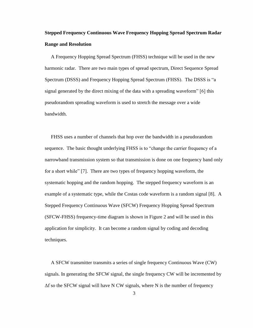
Stepped Frequency Continuous Wave Frequency Hopping Spread Spectrum Radar

Range and Resolution

A Frequency Hopping Spread Spectrum (FHSS) technique will be used in the new

harmonic radar. There are two main types of spread spectrum, Direct Sequence Spread

Spectrum (DSSS) and Frequency Hopping Spread Spectrum (FHSS). The DSSS is “a

signal generated by the direct mixing of the data with a spreading waveform” [6] this

pseudorandom spreading waveform is used to stretch the message over a wide

bandwidth.

FHSS uses a number of channels that hop over the bandwidth in a pseudorandom

sequence. The basic thought underlying FHSS is to “change the carrier frequency of a

narrowband transmission system so that transmission is done on one frequency band only

for a short while” [7]. There are two types of frequency hopping waveform, the

systematic hopping and the random hopping. The stepped frequency waveform is an

example of a systematic type, while the Costas code waveform is a random signal [8]. A

Stepped Frequency Continuous Wave (SFCW) Frequency Hopping Spread Spectrum

(SFCW-FHSS) frequency-time diagram is shown in Figure 2 and will be used in this

application for simplicity. It can become a random signal by coding and decoding

techniques.

A SFCW transmitter transmits a series of single frequency Continuous Wave (CW)

signals. In generating the SFCW signal, the single frequency CW will be incremented by

Δf so the SFCW signal will have N CW signals, where N is the number of frequency

4

steps with each single frequency step equal to fn=f0 +(N-1) Δf, where Δf is the frequency

difference between two successive frequencies. Each frequency will be transmitted for a

short time equal to the dwell time (Δt).

Figure 2 Stepped Frequency Continuous Wave -Frequency Hopping Spread Spectrum

SFCW-FHSS frequency-time diagram

With a single measurement of the SFCW radar, assuming the target was at distance

R0, the phase of the backscattered wave will be proportional to the distance R0 as given

below:

(1)

5

where E is the scattered electric field, A is the scattered field amplitude, k is the wave

number corresponding to the frequency vector (fo, f1, f2,…..fN) and it is equal to /

where λ is the wavelength which is equal to the speed of light (c) over the frequency (f)

and the number 2 is there because the signal is going back and forth [9].

Equation (1) is only for a single frequency step while the SFCW signal can be

represented by a discrete function equal to:

∑

(2)

It is possible to calculate the distance R0, by taking the inverse Fourier transform (IFT) of

the output of the SFCW radar. The resulting time-domain signal will be an impulse

response which has a peak corresponding to the target distance [10].

The range resolution of the SFCW radar system depends on the bandwidth and this

can be represented as:

(3)

while the Maximum unambiguous Range resolution of the SFCW radar is:

(4)

Where Δf is the frequency difference between two successive frequencies and it is equal

to the bandwidth divided by the number of frequency steps (N) so:

(5)

6

It can be noticed that a higher resolution requires more bandwidth and for longer

maximum unambiguous ranges the number of frequency steps (N) should increase [11]

[9] [14]. Equations (1), (2), (3) and (4) above are only valid for a typical radar system

and they should be modified for the harmonic radar case.

Harmonic Radar Range Equation

The operation of harmonic radar is not described by the radar range equation [15]

since the frequency conversion is not accounted for. A more accurate description

involves the use of Friis transmission equation for both the forward and return paths [5]

as follow: If a transmitter is transmitting a power Pt with an isotropic antenna then the

power density Wo is:

(6)

where the surface area of the sphere ( and R is the distance between the target

and the transceiver. If a directional antenna is used instead of an isotropic one, then the

power density at a point in space is modified by the power gain of the antenna in that

direction, G(Ө,φ) where Ө and φ define the principle plane angles from the main beam of

the antenna. Considering the simplest case for a target in the main beam of the radar

[17], the power density is defined as:

(7)

The transmitting power at the receiver side is:

7

(8)

where the surface area , is the receiving antenna gain and is the

wavelength. Substituting W0 in (8) with its value in (7) yields the overall Friis equation:

=

(9)

The Friis transmission equation relates the power received (Pr) to the power

transmitted (Pt) between two antennas separated by a distance R > 2D2/λ, where D is the

largest dimension of either antenna [16]. It should be noted that, higher transmitted

power, higher gain antennas, lower frequency and shorter distances between antennas are

required for higher received power.

The harmonic radar range equation was developed in a fashion that is similar to the

conventional radar range equation except that harmonic cross-section was substituted for

radar cross-section in [5]. Cross sectional area is a good method for describing the tag

from a system point of view as in typical radar systems. The harmonic radar tag is a

dipole antenna that is one-half wavelength long at the fundamental frequency and one

wavelength long at the second harmonic frequency. This tag has three functions first, to

capture the incident signal and efficiently deliver it to the frequency conversion stage;

second, the frequency conversion stage is to deliver the maximum second harmonic

power to the transmitting stage; and third, the transmitting stage is to efficiently radiate

8

the second harmonic power back to the receiver [5]. The harmonic cross section of the

tag is defined as:

σh =

(10)

where EIRP is the Effective Isotropic Radiated Power from the tag at the second

harmonic in units of watts and Wf is the fundamental frequency power

incident upon the tag. Assuming an ideal tag with an efficiency of 100 %; that means all

of the fundamental frequency power from the receiving antenna was delivered to the

transmitting antenna at the second harmonic.

(11)

where Ptagh is the power radiated out of the tag at the harmonic frequency and using (6)

Ptagh = Atagf ,where is the fundamental frequency incident power density , Atagf is

the effective area of the tag antenna as a receiver at the fundamental frequency and is

defined by Atagf = Gtagf /4π, Gtagf is the gain of a one-half wavelength dipole and Gtagh

is the gain of a one-wavelength dipole at the harmonic frequency. The ideal harmonic

cross section of the ideal tag using (10) is:

(12)

Using (7), the power density incident upon the tag is given by:

(13)

9

Then, using (10) the EIRP = σh and from (11) the EIRP= PtaghGtagh = R2.

Applying Friis equation (9) on the second harmonic case where the tag is the transmitter

and the harmonic radar transceiver is receiving the signal back from the tag at distance R.

=PtaghGtagh and substituting Ptagh Gtagh from (12) yields:

(14)

Rearranging the equation and solving for the distance R:

√

(15)

Using equation (15) the range performance of a given harmonic radar system can be

predicted.

1.3 Thesis contribution

A stepped frequency continuous wave frequency hopping spread spectrum technique

(SFCW-FHSS) was used to build a laboratory prototype harmonic radar system for the

first time. This technique can detect and estimate the range of a tagged insect. The main

significance of using such a technique is that it can achieve a lower power, lower cost and

lower weight portable harmonic radar system. A mathematical model for the harmonic

radar system that uses the SFCW-FHSS technique was derived, a graphical user interface

MATLAB program was done to simulate the mathematical model and it can be used as a

10

signal processor with the prototype system, the system design and cost was estimated and

the overall prototype system was built and tested.

In this chapter an introduction to the harmonic radar, spread spectrum and radar range

equation was illustrated in general. In the next chapter a mathematical model, parameters

such as range and resolution and an actual design of the new harmonic radar are

presented. In Chapter 3 a simulation of the new harmonic radar system is shown and

discussed and results of various testes are analyzed while in Chapter 4 the harmonic radar

tag is simulated and compared to the old one and finally in Chapter 5 results of testing the

laboratory prototype are presented.

11

Chapter 2

Stepped Frequency Continuous Wave Frequency Hopping Spread Spectrum

Harmonic Radar (SFCW-FHSS) Design

This chapter extends conventional frequency hopping radar to the harmonic radar case

in order to describe range and resolution characteristics.

2.1 System mathematical model range and resolution

Figure 3 Harmonic radar phase shift described in terms of the forward and return paths of

the signal where λ is the wavelength of the fundamental frequency

Comparing with the typical radar system illustrated in the previous chapter, in the

harmonic radar case the forward term corresponding to the phase will not be changed

since the transmitter transmits at the fundamental frequency while the phase

that will accumulate by the signal traveling from the tag to the receiver will be changed

12

from to

. Since the frequency changed to the second harmonic

frequency and the wavelength for this harmonic λh with respect to the fundamental

wavelength λ will be equal to λh =λ/2 .

Equation (1) for a single frequency step will be modified and the new equation will be

as follows:

(16)

And for the stepped frequency signal it will be modified as:

∑

(17)

Taking the Inverse Fourier Transform (IFT) of equation (17) will give the range of the

tag. Let 3 /c = τ then equation (17) becomes:

IFT (E[f]H SFCW)=IFT(∑ )

E[t]H SFCW=∑

It can be seen that the phase is changing with frequency and it is equal to for

equation (17) instead of for equation (2) and the distance R0 will be scaled

back by a 3/c factor for the harmonic case. An important note here is that the time delay

did not change from 2 for the typical radar to 3 for the harmonic radar case as it

may appear from the mathematical point of view, because the distance between the object

and the radar is constant and the speed of light is constant. What changes is the phase

with frequency and thus result in the modification of the scaling factor when calculating

13

the range from 2/c to 3/c. The next step is the range resolution and the maximum

unambiguous range which need modification to include the extra phase shift introduced

by the harmonic.

The transmitted signal at two successive frequencies and of the radar can be

represented as:

(t) =

(t) =

Phases associated with the two frequencies are:

Ө1=

and Ө2=

And the phase difference is:

Phase difference (ΔӨ) =

If Δf = (f2-f1) and R is maximized when ΔӨ = 2π [18] , solving for the maximum

unambiguous range of the harmonic case RmaxH :

(18)

Where the notation H is for the term harmonic, and using equation (5) the range

resolution for a harmonic system will be:

14

(19)

Where BW is the bandwidth of the entire sweep width. Table 1 illustrates the

modifications that have been made on the SFCW typical radar equations in order to use

them in the SFCW harmonic radar case.

Table 1: Typical vs. harmonic SFCW radar

SFCW typical Radar SFCW harmonic radar

Phase

Range Resolution

Maximum Unambiguous

Range

From Table 1 and with all parameters constant the SFCW harmonic radar has a better

range resolution while the typical radar has a longer maximum unambiguous range.

2.2 Parameter selection

Industry Canada permits frequency hopping systems in the band 5725-5850 MHz

where the maximum peak conducted output power shall not exceed 1 W, the EIRP should

not exceed 4 W, and it shall use at least 75 hopping channels and “The average time of

occupancy on any frequency shall not be greater than 0.4 seconds within a 30-second

period” [13].

15

A homodyne receiver was selected to detect the signal coming back from the tag and

signal processing in MATLAB will be used to determine the distance to the tag. The full

125 MHz will be used for 0.8 m resolution while 100 frequency steps were selected for

an 80 m maximum unambiguous range. The dwell time was selected to be 10 ms and the

power will be as close to the 4 W maximum EIRP as possible in order to maximize range

performance. The 10 ms is acceptable for such a laboratory prototype and it was the best

available choice while it should be noted that this is too slow in the field. The field unit

needs to update every 0.1 s so the dwell time would need to be 1 ms.

2.3 The tag

The harmonic radar tag must be very small and light weight so that insects can carry it

while flying. It must also be mechanically robust enough to survive both fitting to an

insect in the field and the abrasion and bending that might be caused by grooming and

foraging activities [20]. As mentioned earlier, the tag can be seen as a transceiver, it

receives the signal at the fundamental frequency and then through the nonlinear Schottky

diode the second harmonic is produced and transmitted through the dipole antenna. A

thin copper wire along with the MA4E2502 low barrier silicon Schottky diode was used

to build this tag in the lab. A tagged insect can be seen in in figure 4.

16

Figure 4 Tagged Colorado potato beetle [5]

The harmonic cross section of the ideal tag using equation 12 is:

=

where the one-half wavelength dipole gain Gtagf =1.64, the one-wavelength dipole Gtagh

=2.41 [19] and which is the wavelength of the smallest frequency of the

selected frequency band and this should be the best case since larger harmonic cross

section means easier to be detected and results better received power and at the same time

larger frequencies yields the shortest wavelength which decreases the received power

based on the Friis formula (14), since the bandwidth is small compared to the frequencies

this should have minor effect. The ideal harmonic cross section at this new radar

frequency is 863.66 mm2 which is larger than the old harmonic radar that works at a

fundamental frequency 9.41 GHz and has a 320 mm2 ideal harmonic cross section and

24.3 mm2 simulated cross section for a 12 mm long dipole [5]. The 320 mm

2 assumes

complete conversion to the second harmonic while the 24.3 mm2 includes conversion

17

losses and is a more realistic value. Taking the same ratio; the simulated cross section for

the tags operating at the new radar frequency is approximately 65.5mm2.

2.4 Stepped Frequency Continuous Wave (SFCW) harmonic radar block diagram

The system design is illustrated in the block diagram of Figure 6; the signal generator

sends a stepped frequency continuous wave of 100 frequency steps in the frequency band

5.725GHz to 5.85GHz at 24dBm power level; each step is sent for a 10 ms dwell time. A

3 dB power divider is used to divide the signal into two paths, the first part of the signal

(level 21 dBm) goes to a frequency multiplier that generates the second harmonic of the

original signal and this multiplier has a 10 dB conversion loss, the output of the multiplier

will be filtered to suppress the fundamental frequency after that the signal enters the local

oscillator port of the IQ mixer. While the other part of the signal passes through a low

pass filter to suppress the second harmonic frequency, this low pass filter suppress the

second harmonic frequency by approximately -24 dBm over the transmitting range and

adds a 1.76 dBm loss on the fundamental, a 17 dBm signal, taking into account the cables

and the low pass filter losses, is transmitted via a transmitting antenna that has a 12 dBi

gain. The receiving antenna that has 19 dBi gain captures the low power signal and

passes it to a high pass filter to suppress the fundamental frequency then to a Low Noise

Amplifier (LNA); this low noise amplifier has 11 dB gain and noise figure equal to 1.8

dB and another high pass filter is added to suppress the fundamental frequency again. An

amplifier with a 13 dB gain is added after that followed by a power limiter (an amplifier

with 19 dB saturated power and an attenuator of 15 dB over the range 0-18GHz) to

protect the IQ mixer RF port in case of high power since the maximum power for this

18

mixer at the RF port is 5 dBm. The reason of adding an amplifier followed by an

attenuator instead of a typical power limiter is the price; it is costly to buy an SMA power

limiter for this laboratory prototype system. Adding an attenuator seems reasonable since

it is a good solution in terms of gain, the effect of this is in the noise since it has a large

noise figure which is equal to the insertion loss and since this comes after amplification it

has a minor effect on the overall noise figure of the system. An alternative solution can

be seen in Figure 5; this type of structure can be used to limit the RF swing to just above

positive Vcc and just below negative Vcc.

Figure 5 Power limiter using two diodes

The IQ mixer has two signals on its ports; the received signal at the second harmonic on

its RF port and the second harmonic from the transmitter on the LO port. The mixed

signals yield a zero IF in phase (00) signal on IF1 and a quadrature phase (90

0) signal on

19

port IF2, this mixer has 11 dB of conversion gain. Since this is a homodyne receiver, the

output of the mixer has two DC components, in phase and quadrature phase signals,

corresponding to the phase difference. By sweeping the frequency over the 100 steps this

complex signal can be converted to the time domain using the inverse Fourier transform

and the speed of light; from that the distance to the tag can be calculated. The output of

the IQ mixer passes through audio amplifiers followed by a low pass filter (LPF) then an

oscilloscope is used to detect that analog signal and convert it to a digital signal that can

be processed later using MATLAB to calculate the range.

Figure 6 The complete new SFCW harmonic radar system block diagram with the

transmitter, the tag and the receiver

IQ mixer

LPF

Tag

f1f1

2f12f1

MA

TLA

B

Power

LimiterAmplifier

HPF

Block f1LNARFRF

HPF

Bock f1

Signal

generator

Power

divider

Freq.

Mul(x2)

Transmitting

antenna

Filter block

2f1

LOLO

ADC

LPF ADC

HPF

Block f1

Receiving

antenna

Amp. Amp.

I dataI data Q dataQ data

20

Figure 7 Signal processing technique that is used in MATLAB to calculate the range

The oscilloscope records a text file that has 50 thousand points and since 100 frequency

steps are transmitted each 500 points in the file correspond to one frequency step. In

MATLAB an average of the 500 voltage levels is taken and then assigned to its

frequency step and since each step is transmitted for a dwell time equal to 10 ms this is

like low pass filtering with a 100 Hz filter. After that, an inverse Fourier transform for

the 100 frequency steps with their averages is applied to calculate the range. Figure 6

illustrates this process. The actual components of the designed system are presented in

Table 2.

Averaging I dataI data

Add

Averaging Q dataQ data

Complex signalComplex signal IFT Range

21

Table 2: Actual components

Components Information

Signal Generator Agilent PSG E8257C

Oscilloscope (ADC) Wave pro 950

Power divider Omni Spectra FSC 16179

LPF CLPFL-0100

HPF VH-8400 + SMA

LNA Hittite HMC564LC4

Amplifier AVA-183A+

Attenuator (x-band) MIDWEST MICROWAVE ATT-0290-15-

SMA-02

IQ Mixer Hittite HMC908LC5

Audio amplifier (DC-Signal) Harrison 6824 A power supply-Amp.

Frequency multiplier ZX-2-24-S+

System Gain (G) and Noise Figure (NF)

The stepped frequency continuous wave SFCW harmonic radar receiver is illustrated

in Figure 8. The total gain of this cascaded system can be found by simple summation of

the gain values in dB of each stage as follow [21]:

22

∑

(20)

Where N is the number of stages and it is equal to 10 in this system. The noise figure of

this system is calculated as follows [21]:

NF total = +

+

+

+……+

(21)

Where N.F1 is the noise figure of the first stage and G1 is the gain of the first stage and

so on up to the last stage. It can be seen from equation (22) that the first stage is the most

important stage in the system and the receiving antenna should be connected with a short

wire to the next stage because losses in the beginning are not divided by the gain and thus

result in larger noise figure values.

Figure 8 The SFCW harmonic radar receiver block diagram

Noise figures and gains values of the components are illustrated in Table 3; the noise

figure value of the audio amplifier was not available and it was assumed to be 6 dB and it

HPF HPFLNA Amplifier AttenuatorIQ

Mixer

Audio

amplifier

Audio

amplifier LPFAmplifier

Rx

ADC

23

has a minor effect because it is at the 8th

and 9th

stages as in Figure 7 and their values are

divided by all the previous gains. Using values in Table 3, equations (20) and (21); the

overall system noise figure is equal to 3.7 dB and the total gain is 67 dB.

Table 3: Actual components gains and noise figures values

Components Gain(dB) NF(dB) Gain(Linear) NF(linear)

HPF -1.2 1.2 0.7586 1.3183

LNA 11 1.8 12.5893 1.5136

HPF -1.2 1.2 0.7586 1.3183

Amplifier 13 4.8 19.9526 3.02

Amplifier 13 4.8 19.9526 3.02

Attenuator -15 15 0.0316 31.6228

IQ mixer 11 2.2 12.5893 1.6596

Audio amplifier 18.45 6 70 3.94

Audio amplifier 18.45 6 70 3.94

LPF -0.36 0.36 0.9204 1.0864

2.4 Radar range equation

The range equation is a theoretical approach that helps in estimating the maximum

detectable range of a radar system. The harmonic radar range equation was developed in

a fashion that is similar to the conventional radar; this was illustrated in equation (15) in

Chapter 1 as follows:

24

√

(22)

Where, is the transmitted power, is the harmonic cross section, Gt is the

transmitting antenna gain, Gr is the receiving antenna gain, is the wavelength of the

harmonic frequency and Pr is the minimum power that can be detected by the receiver.

A receiver can be represented as a black box with known total gain and noise figure as in

in figure 9. In order to calculate the sensitivity of the receiver, the noise power of the

system should be calculated. The noise power (Pn) is defined as [21]:

(23)

Where, K is the Boltzman's Constant = 1.38 x10-23

joules/kelvin, T is the temperature in

Kelvin and B is the 3 dB noise bandwidth. It can be seen that larger bandwidth adds

more noise to the system so having the final IF bandwidth as narrow as possible is

important. As mentioned earlier the averaging was taken in MATLAB for every dwell

time of 10 ms which is equal to low pass filtering with a 100 Hz bandwidth. The overall

noise temperature ( ) can be obtained using the overall system noise figure as follow:

NF (dB) =10xlog (1+

)

= (

-1)

(24)

25

Where NF is the total noise figure of the receiver and it is equal to 3.70 dB, T0 is a

constant or a standard temperature and it is equal to 290 Kelvin. Using equation (24) the

noise temperature is equal to 389.8 K. Using this noise temperature value, 100 Hz

bandwidth and equation (23) the noise power is equal to -182.7 dBw. So for a signal to

be received it should be above this level and if the signal to noise ratio is assumed to be

10 dB the receiver sensitivity is:

Pmin = KTB+ signal to noise ratio

Using 65.5 mm2 harmonic cross section, 17 dBm transmitted power (Pt), transmitting

antenna gain (Gt) =12dBi, receiving antenna gain (Gr) =19 dBi and Pmin =-172.7 dBw the

maximum detectable range as in (15) is equal to 127.7 m.

The noise power limits the maximum detectable range of the radar since it limits the

system sensitivity but this is not the only factor; for example the maximum unambiguous

range of the system is 80 m and this limits the range.

Figure 9 The harmonic radar receiver

A 950 LeCroy WavePro oscilloscope is used as an Analog to Digital Converter

(ADC); this device can detect a signal as low as -38 dBm. As in Figure 9, the total system

gain is 67 dB so the minimum signal that can be detected by this ADC is -67dB-

Gain=67 dB

Noise figure=3.7 dB

Rx

ADC

26

38dBm=-105 dBm. Changing the Pmin to -105 dBm instead of -172.7 dBw or (-142.7

dBm) and using equation (15) with all other parameters retaining their same values yields

a maximum detectable range of 14.5 m.

The other factor affecting the detectable range is the self-interference; in the optimal

case, the SFCW harmonic radar should detect the presence of the target when there is one

and should detect nothing when there is no tag. Unfortunately, this is not the case since

even when there is no tag this system detects a peak at the second harmonic frequency

because of the self-interference. This problem has been taken into account while building

the system and in the next section the shielding process to minimize the self-interference

effect is presented.

In summary, the maximum detectable range of this harmonic radar is limited by one of

these: the noise power, the maximum unambiguous range, the analog to digital converter

sensitivity and the self-interference.

2.5 Assembling the system

First, tags were fabricated in the laboratory using copper coated steel wire AWG#34

along with the MA4E2502 low barrier silicon Schottky diode as in Figure 10 then

components were assembled based on the design in Figure 6. The first test showed that

there is a strong signal coming without tag presence because of the self-interference as

indicated earlier, because of that an absorber was placed above the IQ mixer to bring the

signal level down and chokes were placed on the coaxial cables. This brought the signal

level down a little bit and it was not a good solution since it was not stable and practical.

In order to deal with the self-interference problem a shielding process must be done.

27

The system in Figure 6 should be shielded as in Figure 11 to prevent signal leaking

between wires; the signal is leaking in all wires and this includes power supply wires.

Components were placed inside an enclosure and power supply wires were mounted to

the top side of the enclosure using feed-through capacitors and then power supply wires

were soldered with the capacitors ends as in Figure 12, the edges of the enclosures were

taped using copper tape to make sure that leaking is prevented as much as possible. The

shielded box 1 has the low noise amplifier, the X-band amplifiers and the attenuator as in

Figure 13; the high pass filter was placed outside of it since there is no space available for

it. Shielded box 2 has the frequency multiplier, the high pass filter and the IQ mixer as in

Figure 14 and a voltage regulator was built to maintain constant voltage levels for the

amplifiers and IQ mixer as in Figure 16.

Figure 10 Harmonic radar tags

28

Figure 11 The shielded SFCW harmonic radar system block diagram

Figure 12 Power supply wires mounted to feed-through capacitors in the enclosure

IQ mixer

LPF

Tag

f1f1

2f12f1

MA

TLA

B

Power

LimiterAmplifier

HPF

Block f1LNARFRF

HPF

Bock f1

Signal

generator

Power

divider

Freq.

Mul(x2)

Transmitting

antenna

Filter block

2f1

LOLO

ADC

LPF ADC

HPF

Block f1

Receiving

antenna

Amp. Amp.

I dataI data Q dataQ data

Shielded box 1

Shielded box 2

29

Figure 13 Shielded box 1 that has the low noise amplifier, the X-band amplifiers and the

attenuator

Figure 14 Shielded box 2 that has the frequency multiplier, the high pass filter and the IQ

mixer

30

The overall system is seen in Figure 15. After the shielding process is done and

measuring before the IQ mixer input using a spectrum analyzer the signal level went

down by 40 dB then another test was performed using MATLAB to determine the

impulse response with a peak corresponding to the tag position; the results showed that

there is more than one peak corresponding to the reflection and these peaks are presented

both with and without the tag. The MATLAB algorithm was modified as in Figure 17 so

that the I and Q data are collected with no tag as a reference and with tag, the two

complex numbers are subtracted to eliminate the common self-interference signal then

the inverse Fourier transform is used to estimate the range.

Figure 15 The SFCW harmonic radar inside the anechoic chamber with all components

indicated

31

Figure 16 Voltage regulator that was made to provide a constant voltage level for the

amplifiers in order to protect them

Figure 17 MATLAB algorithm after modification so that the two signals with and

without the tag are subtracted before the inverse Fourier transform

Averaging I dataI data

Add

Averaging Q dataQ data

Complex signalComplex signal

IFT Range

Averaging I data

no tag

I data

no tag

Add

Averaging Q data

no tag

Q data

no tag

Complex signalComplex signal

Subtract

32

2.6 Conclusion

The SFCW technique was used to build a harmonic radar system for the first time in

order to achieve the lower power and lower cost goal. The mathematical model was

modified for the harmonic radar and different parameters such as range and resolution

were modified as well. The system was designed, actual components models were

selected, the MATLAB algorithm was developed and the entire system was assembled

and tested.

33

Chapter 3

SFCW Harmonic Radar Simulation

The mathematical model that was derived in the previous chapter for the harmonic

radar is simulated using MATLAB. First, the IQ data is generated as in figure 18; it

represents how the phase is changing with the frequency sweep. If the frequency is not

changing, the IQ data will be constant and the distance cannot be obtained. As the

distance between the tag and the transceiver increases more phase change is seen as in

Figure 19. The frequency band that was used in this simulation is 5.725 GHz-5.85 GHz

with 100 frequency steps, this results in a 0.8 m range resolution and 80 m maximum

unambiguous range. Second, the IQ data is added yielding a complex number as in

Figure 20 that represents the electric field that was illustrated in the previous chapter as:

∑

(25)

It can be seen that this complex number makes a perfect circle since there is no noise

added to the signal. Taking the inverse Fourier transform of this complex number results

in a peak corresponding to the tag position as in Figure 21 for a distance R=1.3 m. The

distance that is measured for this simulation is an integer multiple of the range resolution;

for example if the distance from the tag is 1.3 m the calculated distance will be 1.6 m

which is the closest range resolution as in Table 4. The impulse response for the 10.4 m

case is in Figure 22 and it has a sharper peak than in the 1.3 m case since there is no error

in calculating this value and this distance is an integer multiple of the range resolution. It

34

can be noticed that when the distance R is at the edge such as 1.2 m it results in two peak

values as in Figure 23.

Figure 18 IQ data for distance R=1.3 m

Figure 19 IQ data for distance R=10.4 m

35

Figure 20 Real part vs. imaginary part of the electrical field

Figure 21 Impulse response for distance R=1.3 m

36

Figure 22 Impulse response for distance R=10.4 m

Figure 23 Impulse response for distance R=10 m

37

Table 4: Range estimation based on multiples of the range resolution

Real distance Measured distance

0 < distance<4.0 4

4.0 < distance<1.2 0.8

1.2 0.8 or 1.6

1.2 < distance<2 2.1

2 1.6 or 2.4

2 < distance<2.8 2.0

n-0.4< distance<n+0.4

;where n = m*0.8 and m is an integer

n

The range resolution as mentioned earlier depends on the bandwidth; for the distance

R=1.3 m the measured distance was equal to 1.6 m and if a larger bandwidth is used a

close value to it could be reached as in Figure 24; the bandwidth was increased to 600

MHz instead of 125 MHz yielding 0.167 m range resolution. Range resolution can be

improved using zero padding as well, adding 100 zeros to the IQ data as in Figure 25 will

not add any new information about the phase since it is not changing and has a constant

zero value but that will fake the range resolution as in Figure 26 for the same distance; it

should be noted that this is not as clear a peak as in Figure 24 as the energy of the signal

is spread across a wider bandwidth.

38

Figure 24 Impulse response at distance R=1.3 and bandwidth=600 MHz

Figure 25 Zero padded IQ data with a 100 zeros for R=1.3 m

39

Figure 26 Zero padded data with 100 zeros for distance R=1.3 m

The maximum unambiguous range of this system is 80 m assuming a 100 frequency

steps is used and this yields a 1.25 MHz frequency difference between two successive

frequencies Δf. This limits the maximum detectable range of the system; for example if

the distance R= 80 m the simulation will not detect this distance and the maximum

detectable range is 78.4 as in Figure 27; the maximum unambiguous range can be

increased by increasing the number of frequency steps while keeping the bandwidth the

same. Changing the frequency steps from 100 steps to 200 steps yields 160.7 m

maximum unambiguous range and then distances like 120 m can be detected as in Figure

28.

40

Figure 27 Impulse response at distance R=78.8 m

Figure 28 Impulse response at distance R=120 m

41

The last part of the simulation involves adding noise to the system; if noise is added to

the IQ data as in Figure 29 to simulate the real life measurements, the circle

corresponding to the electric field is not perfect anymore as in Figure 30 and the range

cannot be estimated as in Figure 31. Increasing the Signal to Noise Ration SNR of the

system as in Figure 32 makes it possible to measure the range as in figure 34 while the

noisy circle is still not perfect but it takes a better shape as in figure 33. A GUI was built

for simulation and it is also used as a signal processor since you can load ADC data into

it as in Figure 35.

Figure 29 Noisy IQ data with low SNR

42

Figure 30 Real part vs. imaginary part of the electrical field

Figure 31 Impulse response for low SNR

43

Figure 32 IQ data with 10 dB SNR

Figure 33 Real part vs. imaginary part of the electrical field for 10 dB SNR

44

Figure 34 Impulse response at distance R=1.3 m for 10 dB SNR

45

Figure 35 MATLAB GUI program

46

Chapter 4

Harmonic Radar Tag Simulation

The Method Of Moments Simulation

This harmonic radar simulation was done to determine the performance of the tag. A

method of moments simulation was used to simulate the wire dipole antenna for both

SFCW and pulsed harmonic radar; it breaks the antenna into several pieces and evaluates

antennas parameters using the contribution of current in each pieces summation. The

4nec2 software was used to do the method of moments simulation. This simulation gives

important information such as the gain, the radiation pattern and the input impedance of

the dipole antenna for different frequencies. A copper wire that has the same radius as

the AWG#34 wire is simulated as in Figure 36; this wire is a half-wavelength dipole

antenna at the fundamental frequency and a full-wavelength dipole antenna at the second

harmonic. The dipole antenna has an isotropic radiation pattern as in Figure 37 and

Table 5 illustrates the input impedance , the gain, the radiation resistance and resistance

losses for the pulsed harmonic radar which works at a fundamental frequency equal to

9.41GHz and the SFCW harmonic radar which works at a fundamental frequency equal

to 5.725 GHz ; although it is actually a frequency hopping technique and it is hopping

over the 125 MHz but for simplicity the first frequency channel was taken and the rest

should give almost the same results since the difference in frequency is relatively small.

In addition, the tag was fabricated to be a half-wave dipole antenna at this frequency.

47

Figure 36 Dipole antenna as in 4nec2 software

Figure 37 Electric field patterns as in 4nec2

48

Table 5: Method of moments simulation results for the pulsed harmonic radar and the

SFCW radar

Old system New system

Tx Rx Tx Rx

Frequency

(GHz)

9.41 18.82 5.725 11.45

Gain

(dBi)

2.15 3.95 2.13 3.92

Input impedance

(Ω)

88.10+j50 873-j530 85.6-j48.60 1219-j564

Radiation resistance

(Ω)

86.90 872.30 85.15 1217.40

Losses resistance

(Ω)

1.20 0.70 0.45 1.60

The Harmonic Balance Simulation

The input impedance of the dipole antenna is taken from the method of moments

simulation to be used in this simulation using Agilent ADS software. The tag can be

modeled in terms of its Thevenin equivalent circuit as in Figure 38 [5]; a conjugate

matched half-wavelength dipole will receive a 1.26 mW signal from a 4 kW (peak pulse)

radar located at a range of 100 m operating at 9.41 GHz with an antenna gain of 24.5 dBi

using Friis equation (14). Given a half-wavelength dipole impedance of 73+j42.5 Ω, the

peak voltage of the equivalent source was set to 607 mV. While for the SFCW harmonic

radar with the same conditions but changing the operating frequency to 5.725 GHz, the

transmitted power to 4 W and the antenna gain to 12 dBi the peak voltage of the

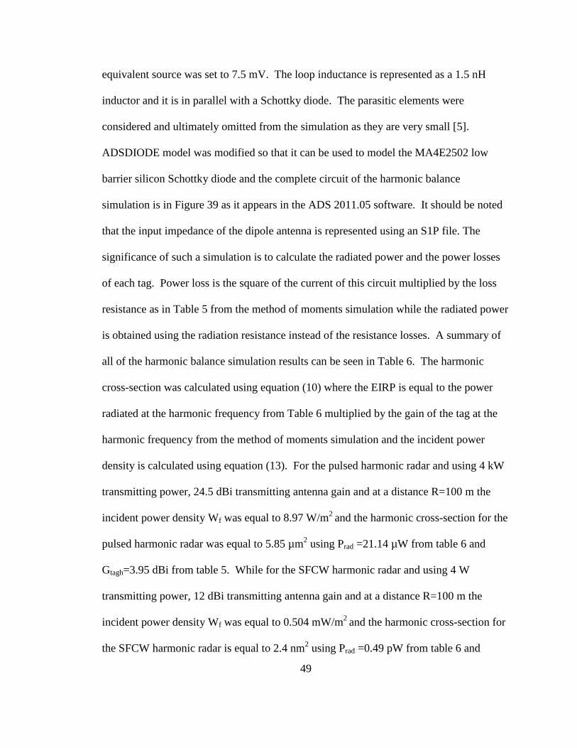
49

equivalent source was set to 7.5 mV. The loop inductance is represented as a 1.5 nH

inductor and it is in parallel with a Schottky diode. The parasitic elements were

considered and ultimately omitted from the simulation as they are very small [5].

ADSDIODE model was modified so that it can be used to model the MA4E2502 low

barrier silicon Schottky diode and the complete circuit of the harmonic balance

simulation is in Figure 39 as it appears in the ADS 2011.05 software. It should be noted

that the input impedance of the dipole antenna is represented using an S1P file. The

significance of such a simulation is to calculate the radiated power and the power losses

of each tag. Power loss is the square of the current of this circuit multiplied by the loss

resistance as in Table 5 from the method of moments simulation while the radiated power

is obtained using the radiation resistance instead of the resistance losses. A summary of

all of the harmonic balance simulation results can be seen in Table 6. The harmonic

cross-section was calculated using equation (10) where the EIRP is equal to the power

radiated at the harmonic frequency from Table 6 multiplied by the gain of the tag at the

harmonic frequency from the method of moments simulation and the incident power

density is calculated using equation (13). For the pulsed harmonic radar and using 4 kW

transmitting power, 24.5 dBi transmitting antenna gain and at a distance R=100 m the

incident power density Wf was equal to 8.97 W/m2

and the harmonic cross-section for the

pulsed harmonic radar was equal to 5.85 µm2 using Prad =21.14 µW from table 6 and

Gtagh=3.95 dBi from table 5. While for the SFCW harmonic radar and using 4 W

transmitting power, 12 dBi transmitting antenna gain and at a distance R=100 m the

incident power density Wf was equal to 0.504 mW/m2

and the harmonic cross-section for

the SFCW harmonic radar is equal to 2.4 nm2 using Prad =0.49 pW from table 6 and

50

Gtagh=3.92 dBi from table 5. This means that at a distance of 100 m the pulsed harmonic

radar system has a better harmonic cross-section than the SFCW one since larger

harmonic cross section means easier to be detected. The cost of using lower power is

-33.9 dB difference between the two harmonic cross- sections which is a large cost.

Figure 38 Complete circuit equivalent for the harmonic radar tag

51

Figure 39 Equivalent circuit of the tag at the fundamental frequency of the tag

Table 6: Harmonic balanced simulation results

Frequency

(GHz)

Current

(µA)

Power losses

(W)

Power radiated

(W)

5.725 80.7 2.93 nW 0.55 µW

11.45 0.02 0.64 fW 0.49 pW

9.41 4000 19.20 µW 1.4 mW

18.8 155.7 16.9 nW 21.14 µW

52

Chapter 5

Testing The Laboratory Prototype

The SFCW harmonic radar was tested in the anechoic chamber; the system was

assembled as in Chapter 2, the tag is placed in front of the radar system to simulate a real

tagged insect then the data was collected from the oscilloscope to the computer and it is

processed using the MATLAB GUI program. The collected IQ data from the oscilloscope

for the distance R=0.8 m with the tag presence can be seen in Figure 40 then as

previously done in the simulation this data was low pass filtered in MATLAB as in

Figure 01. The same procedure was repeated with no tag present.

Figure 40 IQ data with tag as it came from the oscilloscope at a distance R=0.8 m

53

Figure 41 IQ data with tag after low pass filtering and assigning each average to a

frequency step at a distance R=0.8 m

The impulse response of the tag was calculated for the IQ data using inverse Fourier

transform as in Figure 42 with no tag and in Figure 43 with the tag; the range cannot be

estimated using the impulse response of the IQ data with the presence of the tag due to

the self-interference noise of the system and its corresponding peaks. The subtraction of

the IQ data with and without the tag followed by an inverse Fourier transform makes it

possible to estimate the range of the tag as in Figure 44. This test was repeated for

different distances as in Figure 45; this figure represents the impulse response of the tag

after the subtraction for 0.8, 1.6, 2.4, 3.2 and 4 m.

54

Figure 42 Impulse response with no tag at a distance R=0.8 m

Figure 43 Impulse response with the tag at a distance R=0.8 m

55

Figure 44 Impulse response with peak corresponding to the tag position at a distance

R=0.8 m

Figure 45 Impulse response of the tag at different distances R=0.8,1.6,2.4,3.2 and 4 m

56

Conclusion

The old system uses a magnetron with 4 kW peak power to transmit a sequence of

short pulses that can be used to measure the range. It costs approximately $10,000 in

parts and it is able to pick up a signal up to 30 meters. The new SFCW harmonic radar

maximum power is 4 W, it costs approximately $3500, it has a lighter weight since the

magnetron was removed and it was able to pick a signal up to 4 meters inside an anechoic

chamber although theoretically it should detect around 14 meters as mentioned earlier,

the reason for that might be because the shielding was not perfect so there is still some

signal leaking causing the self-interference problem. This 4 meters distance was obtained

using a 17 dBm transmitting power and an oscilloscope as an analog to digital converter.

It is recommended to use the full 36 dBm allowable transmitting power and a higher

sensitivity analog to digital converter in order to achieve a good range. More gain was

added before the analog to digital converter but this just saturates the output due to the

self-interference. Using 4 W for the SFCW harmonic radar instead of 4 kW for the pulsed

harmonic radar cost a large price of -33.9 dB difference between the two harmonic cross-

sections at a distance R=100 m which make the tag harder to be detected.

Although this SFCW harmonic radar laboratory prototype has a cheaper price, a lower

power and a lower weight compared to the old pulsed harmonic radar, the maximum

range that was measured by this device is equal to 4 m which does not make it a good

replacement for the old pulsed harmonic radar that is able to pick up a signal that is 30 m

away.

57

References

1. Colpitts, B.G.; Luke, D.M. and Boiteau, G., “Harmonic Radar Identification Tag

for Insect Tracking ,” Electrical and Computer Engineering, 1999 IEEE

Canadian Conference on, vol.2,no. 602 - 605 , May.1999.

2. Agriculture and Agri-Food Canada (2014, September). A closer look at insect

behavior produces new insights into pest control [online]. Available:

http://www.agr.gc.ca/eng/science-and-innovation/research-centres/atlantic-

provinces/potato-research-centre/a-century-of-science/?id=1345559675096.

3. Federal Business Opportunities (2014, September). Harmonic Radar Insect

Tracking System [online]. Available:

https://www.fbo.gov/index?s=opportunity&mode=form&tab=core&id=4c2c5e79

27e84631851b317fa39019e7.

4. Colpitts, B.G.; Luke, D.M. and Boiteau, G., “Harmonic radar for insect flight

pattern tracking ,” Electrical and Computer Engineering, 2000 Canadian

Conference on, vol.1, no. 302 - 306 , Halifax, NS, Mar.2000.

5. B.G. Colpitts and G. Boiteau, “Harmonic Radar Transceiver Design: Miniature

Tags for Insect Tracking,” IEEE Trans. on Antennas and Propagation, vol. 52,

no. 11, Nov. 2004.

6. Don Torrieri, Principles of Spread-Spectrum Communication Systems (2nd

Edition), Springer, New York, 2011.

7. Andreas F. Molisch , Wireless Communications (2nd

edition), Wiley, UK, 2011 .

58

8. Mohinder Jankiraman, Design of Multi-Frequency CW Radars (1st edition),

SciTech, USA, 2007.

9. Caner Ozdemir, Inverse Synthetic Aperture Radar Imaging with MATLAB

Algorithms (1st edition), Wiley, USA, 2012.

10. Ybarra, G.A., “Optimal signal processing of frequency-stepped CW radar data,”

IEEE Trans. on Microwave Theory and Techniques, vol. 43, no. 94-105, Jan.

1995.

11. Teoman Emre Ustun, “Design and development of stepped frequency continuous

waver radar and FIFO noise radar sensor for tracking moving ground vehicles”,

Master’s thesis, The Ohio state University of New, Ohio,USA , 2008.

12. Ding Dahai, “Harmonic Radar Receiver Implemented in FPGA Technology”,

Master’s thesis, University of New Brunswick, Fredericton, New Brunswick,

Canada, 2008.

13. RSS 210 Canada Industry (2014, September). Spectrum Management and

Telecommunications Radio Standards Specification [online]. Available:

https://www.ic.gc.ca/eic/site/smt-gst.nsf/vwapj/rss210-i8.pdf/$FILE/rss210-

i8.pdf.

14. Ahmet S. Turk, Koksal A. Hocaoglu, Alexey A. Verti, Subsurface Sensing (1st

edition), Wiley, USA, 2011.

15. D. M. Pozar, Microwave Engineering (2nd Edition), Wiley, Toronto, ON,

Canada, 1998.

59

16. C. A. Balanis, Antenna Theory: Analysis and Design (3rd Edition), Wiley, New

Jersey, 2005.

17. Eugene F. Knott, John Shaeffer, Michael Tuley, Radar Cross Section (2nd

edition),

Artech House, USA, 2004.

18. John M.Weiss , “Continuous-Wave Stepped-Frequency Radar for Target Ranging

and Motion Detection ,” Department of Mathematics and Computer Science

South Dakota School of Mines and Technology, 2009.

19. W. L. Stutzman and G. A. Thiele, Antenna Theory and Design (2nd

edition),

Wiley, New York, 1998.

20. J. R. Riley and A. D. Smith, " Design Consideration for an Harmonic Radar to

Investigate the Flight of Insects at Low Altitude", Computer and Electronics in

Agriculture, vol. 35, no. 2-3, Aug. 2002.

21. David Pozar, Microwave Engineering ( 4th

edition), Wiley, USA, 2011.

60

Appendix A

MATLAB Code

%--scriptname (guiproject.m) % Author:Omar Alfarra % Id: 3460877 % Date: 2014-April-14 % Description:Calculate range,range resolution and maximum unambiguous

range using collected IQ data and compate that with theoratical

approatch.

function varargout = guiproject(varargin) % GUIPROJECT MATLAB code for guiproject.fig % GUIPROJECT, by itself, creates a new GUIPROJECT or raises the

existing % singleton*. % % H = GUIPROJECT returns the handle to a new GUIPROJECT or the

handle to % the existing singleton*. % % GUIPROJECT('CALLBACK',hObject,eventData,handles,...) calls the

local % function named CALLBACK in GUIPROJECT.M with the given input

arguments. % % GUIPROJECT('Property','Value',...) creates a new GUIPROJECT or

raises the % existing singleton*. Starting from the left, property value

pairs are % applied to the GUI before guiproject_OpeningFcn gets called. An % unrecognized property name or invalid value makes property

application % stop. All inputs are passed to guiproject_OpeningFcn via

varargin. % % *See GUI Options on GUIDE's Tools menu. Choose "GUI allows only

one % instance to run (singleton)". % % See also: GUIDE, GUIDATA, GUIHANDLES

% Edit the above text to modify the response to help guiproject

% Last Modified by GUIDE v2.5 13-Apr-2014 15:56:36

% Begin initialization code - DO NOT EDIT gui_Singleton = 1; gui_State = struct('gui_Name', mfilename, ... 'gui_Singleton', gui_Singleton, ... 'gui_OpeningFcn', @guiproject_OpeningFcn, ... 'gui_OutputFcn', @guiproject_OutputFcn, ...

61

'gui_LayoutFcn', [] , ... 'gui_Callback', []); if nargin && ischar(varargin1) gui_State.gui_Callback = str2func(varargin1); end

if nargout [varargout1:nargout] = gui_mainfcn(gui_State, varargin:); else gui_mainfcn(gui_State, varargin:); end % End initialization code - DO NOT EDIT

% --- Executes just before guiproject is made visible. function guiproject_OpeningFcn(hObject, eventdata, handles, varargin) % This function has no output args, see OutputFcn. % hObject handle to figure % eventdata reserved - to be defined in a future version of MATLAB % handles structure with handles and user data (see GUIDATA) % varargin command line arguments to guiproject (see VARARGIN)

% Choose default command line output for guiproject handles.output = hObject;

% Update handles structure guidata(hObject, handles);

% UIWAIT makes guiproject wait for user response (see UIRESUME) % uiwait(handles.figure1);

% --- Outputs from this function are returned to the command line. function varargout = guiproject_OutputFcn(hObject, eventdata, handles) % varargout cell array for returning output args (see VARARGOUT); % hObject handle to figure % eventdata reserved - to be defined in a future version of MATLAB % handles structure with handles and user data (see GUIDATA)

% Get default command line output from handles structure varargout1 = handles.output;

% --- Executes on button press in Harmo_theo. function Harmo_theo_Callback(hObject, eventdata, handles) a=handles.a; R=handles.R; c=handles.C; f=handles.f; it=a*cos(-2*pi*f*R*3/c); qt=a*sin(-2*pi*f*R*3/c); figure(1) plot(f,it,'r',f,qt,'b')

62

figure(2) Es=it+i*qt;

%Range scaling df=f(2)-f(1); % frequency bandwidth N = length(f); % total stepped frequency points dr = c/(3*N*df); % range resolution R = 0:dr:dr*(N-1); %set the range vector

%plot the data plot(R,abs(ifft(Es))) title('Impulse respose') set (gca, 'FontName', 'Anal', 'FontSize' ,10, 'FontWeight', 'normal') xlabel ( 'Range [m]'); ylabel ( 'Amplitude'); lo=abs(ifft(Es)); le=R; Dishar=le(lo==max(lo(:))); mrange=N*dr; set(handles.D, 'String', num2str(Dishar)) set(handles.re, 'String', num2str(dr)) set(handles.max, 'String', num2str(mrange)) guidata(hObject, handles)

% --- Executes on button press in mea_harmonic. function mea_harmonic_Callback(hObject, eventdata, handles) a=handles.a; R=handles.R; c=handles.C; f=handles.f;

it=a*cos(-2*pi*f*R*3/c); qt=a*sin(-2*pi*f*R*3/c); %it(101:400)=0; %qt(101:400)=0; Es1=it+i*qt;

%Range scaling df=f(2)-f(1); % frequency bandwidth N = length(f); % total stepped frequency points dr = c/(3*N*df); % range resolution R1 = 0:dr:dr*(N-1); %set the range vector

%--------------------------------------------------------- %load the measurements files t=handles.Idata(:,1);%%time for I data received signal s1=handles.Idata(:,2);%%amplitude for I data received signal t0=handles.Ich(:,1);%%time for I data channel signal s0=handles.Ich(:,2);%%amplitude forI data channel signal t2=handles.Qdata(:,1);%%time for the transmitted signal s2=handles.Qdata(:,2);%%amplitude for the received signal

63

t00=handles.Qch(:,1);%%time for Q data channel signal s00=handles.Qch(:,2);%%amplitude for Q data channel signal

figure(1) plot(t,s1,'r',t0,s0,'b') title('IQ tag data before filtering') xlabel ( 'samples [s]'); ylabel ( 'Amplitude(V)'); figure(2) plot(t2,s2,'r',t00,s00,'b') title('IQ no tag data before filtering') xlabel ( 'samples[s]'); ylabel ( 'Amplitude(V)'); %---------------------------------------------------------------- %do the averaging for S1 and store it in X1 V=s1(1:50000); count=1; st=1; en=st+499; while en<50001 x1(count)=mean(V(st:en)); st=st+499; en=en+499; count=count+1; end % do the averaging for s0 and save it in x0 V0=s0(1:50000); count0=1; st0=1; en0=st0+499; while en0<50001 x0(count0)=mean(V0(st0:en0)); st0=st0+499; en0=en0+499; count0=count0+1; end %do the averaging of s00 and store it in x00 V00=s00(1:50000); count00=1; st00=1; en00=st00+499; while en00<50001 x00(count00)=mean(V00(st00:en00)); st00=st00+499; en00=en00+499; count00=count00+1; end

% do the averaging for s2 and store it in X2

V2=s2(1:50000); count2=1; st2=1; en2=st2+499; while en2<50001

64

x2(count2)=mean(V2(st2:en2)); st2=st2+499; en2=en2+499; count2=count2+1; end %plot data a=f b=s1 figure(3) plot(f,x1,'r',f,x2,'b') title('IQ tag data after filtering') xlabel ( 'frequency(Hz)'); ylabel ( 'Amplitude(V)'); figure(4) plot(f,x0,'r',f,x00,'b') title('IQ no tag data after filtering') xlabel ( 'frequency(Hz)'); ylabel ( 'Amplitude(V)');

%plot the Data Es=x1+i*x2;% complex number represinting the phase with tag. Es0=x0+i*x00;%complex number representf the channel without tag. C=Es-Es0; df=f(2)-f(1); % frequency bandwidth N = length(f); % total stepped frequency points dr = c/(3*N*df); % range resolution R = 0:dr:dr*(N-1) %set the range vector l1=abs(ifft(Es)); l2=abs(ifft(Es0)); %--------------------- figure(5) plot(R,l2) title('Impulse response no tag') xlabel ( 'Range [m]'); ylabel ( 'Amplitude(V)'); axis([0 max(R) 0 10] )

%--------------------- figure(6) plot(R,l1) title('Impulse response with tag') xlabel ( 'Range [m]'); ylabel ( 'Amplitude(V)'); axis([0 max(R) 0 15] ) %--------------------- figure(7) l3=abs(ifft(C)); plot(R,l3,'g') title('Impulse respose(after subtraction)') xlabel ( 'Range [m]'); ylabel ( 'Amplitude(V)'); axis([0 20 0 15] ) hold on x=R; y=l3; Dishar=x(y==max(y(:))) mrange=N*dr; set(handles.D, 'String', num2str(Dishar)) set(handles.re, 'String', num2str(dr))

65

set(handles.max, 'String', num2str(mrange)) guidata(hObject, handles)

% --- Executes on button press in typical_theo. function typical_theo_Callback(hObject, eventdata, handles) a=handles.a; R=handles.R; c=handles.C; f=handles.f; it=a*cos(-2*pi*f*R/c); qt=a*sin(-2*pi*f*R/c); Es=it+i*qt;

%Range scaling

df=f(2)-f(1); % frequency resolution N = length(f); % total stepped frequency points dr = c/(N*df); % range resolution R = 0:dr:dr*(N-1); %set the range vector

plot(R,abs(ifft(Es))) title('Impulse respose') set (gca, 'FontName', 'Anal', 'FontSize' ,10, 'FontWeight', 'normal') xlabel ( 'Range [m]'); ylabel ( 'Amplitude'); lo=abs(ifft(Es)); le=R; Distyp=le(lo==max(lo(:))); mrange=N*dr; set(handles.D, 'String', num2str(Distyp)) set(handles.re, 'String', num2str(dr)) set(handles.max, 'String', num2str(mrange)) guidata(hObject, handles)

% --- Executes on button press in meas_typical. function meas_typical_Callback(hObject, eventdata, handles) a=handles.a; R=handles.R; c=handles.C; f=handles.f;

it=a*cos(-2*pi*f*R/c); qt=a*sin(-2*pi*f*R/c); Es1=it+i*qt;

t=handles.Idata(:,1);%%time for the transmitted signal s1=handles.Idata(:,2);%%amplitude for the received signal t2=handles.Qdata(:,1);%%time for the transmitted signal s2=handles.Qdata(:,2);%%amplitude for the received signal %do the averaging for S1 and store it in X1 V=s1(1:50000);

66

count=1; st=1; en=st+499; while en<50001 x1(count)=mean(V(st:en)); st=st+499; en=en+499; count=count+1; end % do the averaging for s2 and store it in X1

V2=s2(1:50000); count2=1; st2=1; en2=st2+499; while en2<50001 x2(count2)=mean(V2(st2:en2)); st2=st2+499; en2=en2+499; count2=count2+1; end

Es=x1+i*x2; df=f(2)-f(1); % frequency resolution N = length(f); % total stepped frequency points dr = c/(N*df); % range resolution R = 0:dr:dr*(N-1); %set the range vector plot(R,abs(ifft(Es)),R,abs(ifft(Es1))) title('Impulse respose') set (gca, 'FontName', 'Anal', 'FontSize' ,10, 'FontWeight', 'normal') xlabel ( 'Range [m]'); ylabel ( 'Amplitude'); lo=abs(ifft(Es)); le=R; Distyp=le(lo==max(lo(:))); mrange=N*dr; set(handles.D, 'String', num2str(Distyp)) set(handles.re, 'String', num2str(dr)) set(handles.max, 'String', num2str(mrange)) guidata(hObject, handles)

function R_Callback(hObject, eventdata, handles) % hObject handle to R (see GCBO) % eventdata reserved - to be defined in a future version of MATLAB % handles structure with handles and user data (see GUIDATA) handles.R= str2num(get(hObject,'String')) guidata(hObject, handles) % Hints: get(hObject,'String') returns contents of R as text % str2double(get(hObject,'String')) returns contents of R as a

double

% --- Executes during object creation, after setting all properties. function R_CreateFcn(hObject, eventdata, handles)

67

% hObject handle to R (see GCBO) % eventdata reserved - to be defined in a future version of MATLAB % handles empty - handles not created until after all CreateFcns

called

% Hint: edit controls usually have a white background on Windows. % See ISPC and COMPUTER. if ispc && isequal(get(hObject,'BackgroundColor'),

get(0,'defaultUicontrolBackgroundColor')) set(hObject,'BackgroundColor','white'); end

function C_Callback(hObject, eventdata, handles) % hObject handle to C (see GCBO) % eventdata reserved - to be defined in a future version of MATLAB % handles structure with handles and user data (see GUIDATA) handles.C= str2num(get(hObject,'String')) guidata(hObject, handles) % Hints: get(hObject,'String') returns contents of C as text % str2double(get(hObject,'String')) returns contents of C as a

double

% --- Executes during object creation, after setting all properties. function C_CreateFcn(hObject, eventdata, handles) % hObject handle to C (see GCBO) % eventdata reserved - to be defined in a future version of MATLAB % handles empty - handles not created until after all CreateFcns

called

% Hint: edit controls usually have a white background on Windows. % See ISPC and COMPUTER. if ispc && isequal(get(hObject,'BackgroundColor'),

get(0,'defaultUicontrolBackgroundColor')) set(hObject,'BackgroundColor','white'); end

function f_Callback(hObject, eventdata, handles) % hObject handle to f (see GCBO) % eventdata reserved - to be defined in a future version of MATLAB % handles structure with handles and user data (see GUIDATA) handles.f= str2num(get(hObject,'String')); guidata(hObject, handles)

% Hints: get(hObject,'String') returns contents of f as text % str2double(get(hObject,'String')) returns contents of f as a

double

68

% --- Executes during object creation, after setting all properties. function f_CreateFcn(hObject, eventdata, handles) % hObject handle to f (see GCBO) % eventdata reserved - to be defined in a future version of MATLAB % handles empty - handles not created until after all CreateFcns

called

% Hint: edit controls usually have a white background on Windows. % See ISPC and COMPUTER. if ispc && isequal(get(hObject,'BackgroundColor'),

get(0,'defaultUicontrolBackgroundColor')) set(hObject,'BackgroundColor','white'); end

function a_Callback(hObject, eventdata, handles) % hObject handle to a (see GCBO) % eventdata reserved - to be defined in a future version of MATLAB % handles structure with handles and user data (see GUIDATA)

handles.a= str2num(get(hObject,'String')) guidata(hObject, handles) % Hints: get(hObject,'String') returns contents of a as text % str2double(get(hObject,'String')) returns contents of a as a

double

% --- Executes during object creation, after setting all properties. function a_CreateFcn(hObject, eventdata, handles) % hObject handle to a (see GCBO) % eventdata reserved - to be defined in a future version of MATLAB % handles empty - handles not created until after all CreateFcns

called

% Hint: edit controls usually have a white background on Windows. % See ISPC and COMPUTER. if ispc && isequal(get(hObject,'BackgroundColor'),

get(0,'defaultUicontrolBackgroundColor')) set(hObject,'BackgroundColor','white'); end

function D_Callback(hObject, eventdata, handles) % hObject handle to D (see GCBO) % eventdata reserved - to be defined in a future version of MATLAB % handles structure with handles and user data (see GUIDATA)

% Hints: get(hObject,'String') returns contents of D as text

69

% str2double(get(hObject,'String')) returns contents of D as a

double

% --- Executes during object creation, after setting all properties. function D_CreateFcn(hObject, eventdata, handles) % hObject handle to D (see GCBO) % eventdata reserved - to be defined in a future version of MATLAB % handles empty - handles not created until after all CreateFcns

called

% Hint: edit controls usually have a white background on Windows. % See ISPC and COMPUTER. if ispc && isequal(get(hObject,'BackgroundColor'),

get(0,'defaultUicontrolBackgroundColor')) set(hObject,'BackgroundColor','white'); end

function re_Callback(hObject, eventdata, handles) % hObject handle to re (see GCBO) % eventdata reserved - to be defined in a future version of MATLAB % handles structure with handles and user data (see GUIDATA)

% Hints: get(hObject,'String') returns contents of re as text % str2double(get(hObject,'String')) returns contents of re as a

double

% --- Executes during object creation, after setting all properties. function re_CreateFcn(hObject, eventdata, handles) % hObject handle to re (see GCBO) % eventdata reserved - to be defined in a future version of MATLAB % handles empty - handles not created until after all CreateFcns

called

% Hint: edit controls usually have a white background on Windows. % See ISPC and COMPUTER. if ispc && isequal(get(hObject,'BackgroundColor'),

get(0,'defaultUicontrolBackgroundColor')) set(hObject,'BackgroundColor','white'); end

function max_Callback(hObject, eventdata, handles) % hObject handle to max (see GCBO) % eventdata reserved - to be defined in a future version of MATLAB % handles structure with handles and user data (see GUIDATA)

% Hints: get(hObject,'String') returns contents of max as text

70

% str2double(get(hObject,'String')) returns contents of max as a

double

% --- Executes during object creation, after setting all properties. function max_CreateFcn(hObject, eventdata, handles) % hObject handle to max (see GCBO) % eventdata reserved - to be defined in a future version of MATLAB % handles empty - handles not created until after all CreateFcns

called % Hint: edit controls usually have a white background on Windows. % See ISPC and COMPUTER. if ispc && isequal(get(hObject,'BackgroundColor'),

get(0,'defaultUicontrolBackgroundColor')) set(hObject,'BackgroundColor','white'); end

% --- Executes on button press in Ich. function Ich_Callback(hObject, eventdata, handles) % hObject handle to Ich (see GCBO) % eventdata reserved - to be defined in a future version of MATLAB % handles structure with handles and user data (see GUIDATA) [filename, pathname] = uigetfile('*.txt') loaddata = fullfile(pathname,filename) handles.Ich=load(loaddata) guidata(hObject, handles)

% --- Executes on button press in tagI. function tagI_Callback(hObject, eventdata, handles) % hObject handle to tagI (see GCBO) % eventdata reserved - to be defined in a future version of MATLAB % handles structure with handles and user data (see GUIDATA)

[filename, pathname] = uigetfile('*.txt') loaddata = fullfile(pathname,filename) handles.Idata=load(loaddata) guidata(hObject, handles)

% --- Executes on button press in Qch. function Qch_Callback(hObject, eventdata, handles) [filename, pathname] = uigetfile('*.txt') loaddata = fullfile(pathname,filename) handles.Qch=load(loaddata) guidata(hObject, handles)

% --- Executes on button press in tagQ. function tagQ_Callback(hObject, eventdata, handles) [filename, pathname] = uigetfile('*.txt') loaddata = fullfile(pathname,filename) handles.Qdata=load(loaddata) guidata(hObject, handles)

71

% --- Executes on button press in cle. function cle_Callback(hObject, eventdata, handles)

% --- Executes on button press in togglebutton1. function togglebutton1_Callback(hObject, eventdata, handles) % hObject handle to togglebutton1 (see GCBO) % eventdata reserved - to be defined in a future version of MATLAB % handles structure with handles and user data (see GUIDATA)

% Hint: get(hObject,'Value') returns toggle state of togglebutton1

% --- Executes on button press in readme. function readme_Callback(hObject, eventdata, handles) % hObject handle to readme (see GCBO) % eventdata reserved - to be defined in a future version of MATLAB % handles structure with handles and user data (see GUIDATA) if strcmpi(get(handles.readme,'string'),'Help') set(handles.readme,'string','Hide Help') set(handles.rm, 'String', 'use these values: R=3.3 for typical

radar or R=1 for Harmonic radar;f=11.45e9:2.5e6:1.16975e10,for typical

radar or f=5.725e9:1.25e6:5.8488e9 for Harmonic radar;speed of

peopadation c=197.3e6 for typical radar and c=3e8 for Harmonic Radar;

feel free for amplitude i.e 119')

else %stop recording set(handles.readme,'string','Help') set(handles.rm, 'String', '')

end % Hint: get(hObject,'Value') returns toggle state of readme

Curriculum Vitae

Candidate’s full name: Omar Yasien Alfarra

Universities attended: Princess Sumaya University for Science and Technology

Degree: Bachelor of Science in Communication Engineering

Place: Jordan

Date: Feb.2012