microsoft excel 2010 - kennesaw state university excel 2010 ... excel's formula auditing...

Microsoft Excel 2010 Level 3

2

Copyright © 2010 KSU Department of Information Technology Services

This document may be downloaded, printed, or copied for educational use without further permission of the

Information Technology Services Department (ITS), provided the content is not modified and this statement is

not removed. Any use not stated above requires the written consent of the ITS Department. The distribution of a

copy of this document via the Internet or other electronic medium without the written permission of the KSU -

ITS Department is expressly prohibited.

Published by Kennesaw State University – ITS 2010

The publisher makes no warranties as to the accuracy of the material contained in this document and therefore is

not responsible for any damages or liabilities incurred from its use.

Microsoft product screenshot(s) reprinted with permission from Microsoft Corporation.

Microsoft, Microsoft Office, and Microsoft Access are trademarks of the Microsoft Corporation.

3

Excel 2010 Level 3

Table of Contents

Introduction ............................................................................................................................... 3

Learning Objectives .................................................................................................................. 4

Using Macros ............................................................................................................................ 5

Recording a Macro ................................................................................................................ 5

Running a Macro ................................................................................................................... 7

Editing a Macro ..................................................................................................................... 8

Advanced Formulas .................................................................................................................. 9

Using Insert Function and the Formula Palette ..................................................................... 9

Creating Nested Functions................................................................................................... 10

Auditing Worksheets .............................................................................................................. 11

Using Database Functions....................................................................................................... 14

Creating a List ..................................................................................................................... 14

Using a Form to Enter Data ................................................................................................. 15

Finding a Record ................................................................................................................. 17

Sorting a List ....................................................................................................................... 17

Sorting by One Field ............................................................................................................ 17

Sorting by Multiple Fields ................................................................................................... 18

Filtering Data in a List ......................................................................................................... 19

Analyzing Data with Pivot Tables .......................................................................................... 19

Creating Templates ................................................................................................................. 21

Moving and Copying Worksheets .......................................................................................... 22

Linking Data ........................................................................................................................... 22

Adding a Comment to a Cell .................................................................................................. 23

Sharing Workbooks ................................................................................................................ 24

Tracking Changes ................................................................................................................... 25

Creating and Merging Copies ................................................................................................. 27

Protecting Workbooks and Worksheets .................................................................................. 28

Protecting Cells.................................................................................................................... 28

Protecting Worksheets ......................................................................................................... 29

Protecting Workbooks ......................................................................................................... 30

Limiting Access to Shared Workbooks .................................................................................. 30

Sparklines .................................................................................................................................31

Slicer ........................................................................................................................................32

4

Introduction

Although this is an advanced level document, the material is no more difficult to master than

most of the beginning and intermediate level concepts. You will learn timesaving features

such as macros and templates that will make your work easier and you will learn the quickest

way to troubleshoot problems with your spreadsheets.

Learning Objectives

Automating repetitive tasks with macros

Saving time with templates

Using Excel as a database

Analyzing data with pivot tables

Auditing worksheets

Sharing workbooks over a network

Using Sparklines and Slicer

5

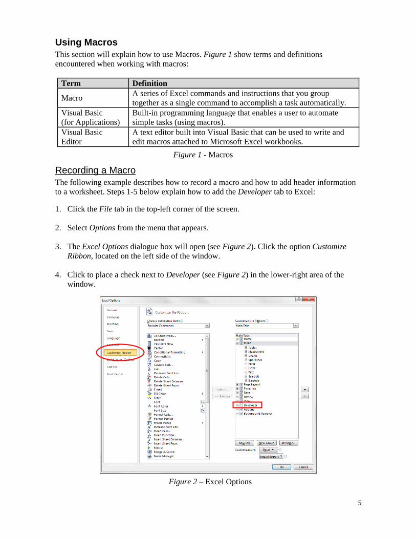
Using Macros

This section will explain how to use Macros. Figure 1 show terms and definitions

encountered when working with macros:

Term Definition

Macro A series of Excel commands and instructions that you group

together as a single command to accomplish a task automatically.

Visual Basic

(for Applications)

Built-in programming language that enables a user to automate

simple tasks (using macros).

Visual Basic

Editor

A text editor built into Visual Basic that can be used to write and

edit macros attached to Microsoft Excel workbooks.

Recording a Macro

The following example describes how to record a macro and how to add header information

to a worksheet. Steps 1-5 below explain how to add the Developer tab to Excel:

1. Click the File tab in the top-left corner of the screen.

2. Select Options from the menu that appears.

3. The Excel Options dialogue box will open (see Figure 2). Click the option Customize

Ribbon, located on the left side of the window.

4. Click to place a check next to Developer (see Figure 2) in the lower-right area of the

window.

Figure 1 - Macros

Figure 2 – Excel Options

6

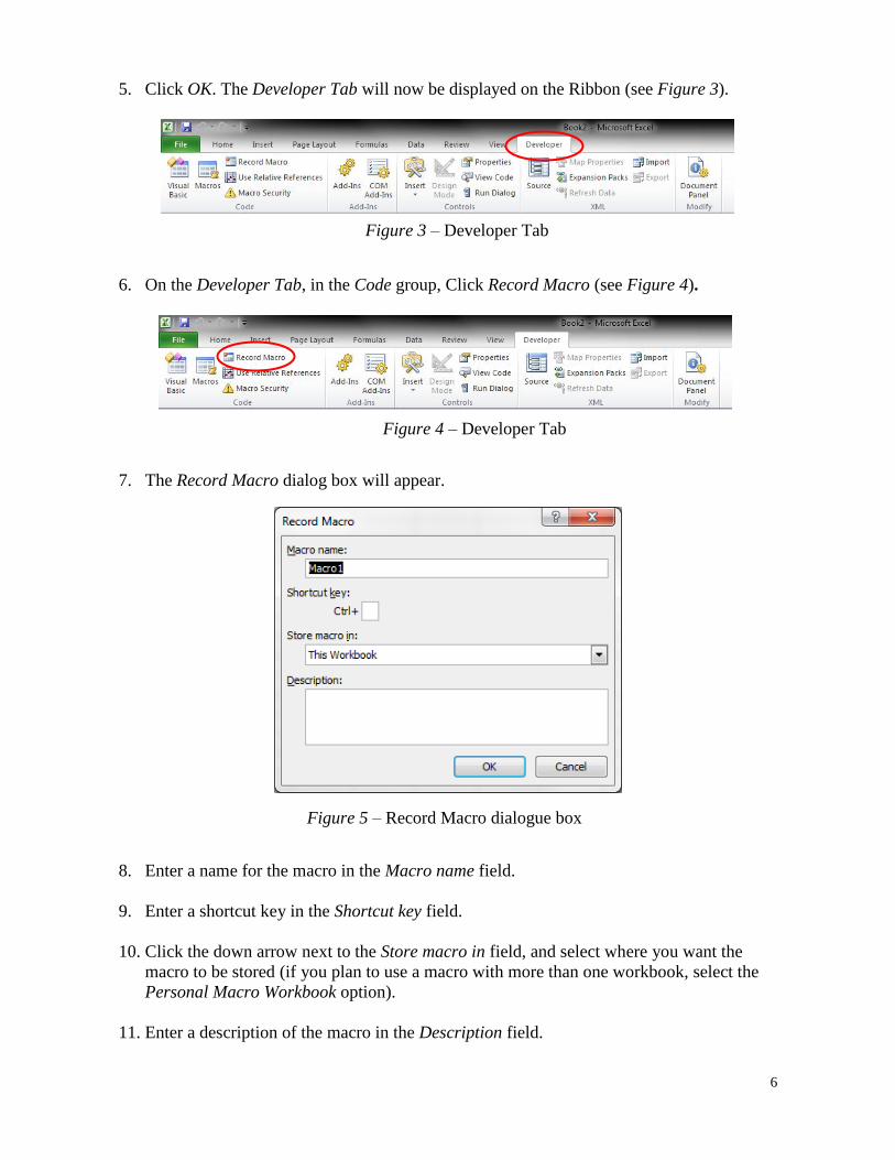
5. Click OK. The Developer Tab will now be displayed on the Ribbon (see Figure 3).

6. On the Developer Tab, in the Code group, Click Record Macro (see Figure 4).

7. The Record Macro dialog box will appear.

8. Enter a name for the macro in the Macro name field.

9. Enter a shortcut key in the Shortcut key field.

10. Click the down arrow next to the Store macro in field, and select where you want the

macro to be stored (if you plan to use a macro with more than one workbook, select the

Personal Macro Workbook option).

11. Enter a description of the macro in the Description field.

Figure 3 – Developer Tab

Figure 4 – Developer Tab

Figure 5 – Record Macro dialogue box

7

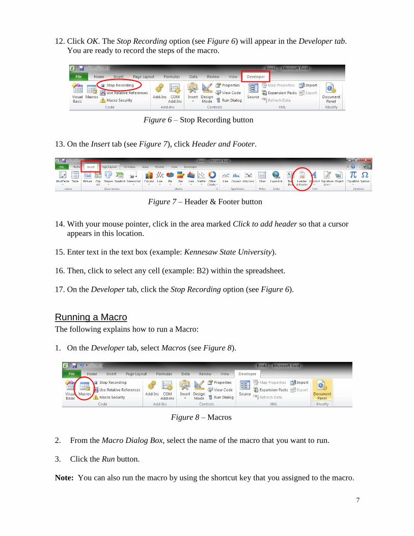
12. Click OK. The Stop Recording option (see Figure 6) will appear in the Developer tab.

You are ready to record the steps of the macro.

13. On the Insert tab (see Figure 7), click Header and Footer.

14. With your mouse pointer, click in the area marked Click to add header so that a cursor

appears in this location.

15. Enter text in the text box (example: Kennesaw State University).

16. Then, click to select any cell (example: B2) within the spreadsheet.

17. On the Developer tab, click the Stop Recording option (see Figure 6).

Running a Macro

The following explains how to run a Macro:

1. On the Developer tab, select Macros (see Figure 8).

2. From the Macro Dialog Box, select the name of the macro that you want to run.

3. Click the Run button.

Note: You can also run the macro by using the shortcut key that you assigned to the macro.

Figure 6 – Stop Recording button

Figure 7 – Header & Footer button

Figure 8 – Macros

8

Editing a Macro

The following explains how to edit a macro:

1. On the Developer tab, select Macros (see Figure 8).

2. From the Macro dialog box, select the name of the macro that you want to edit.

3. Click the Edit button.

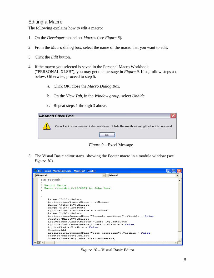
4. If the macro you selected is saved in the Personal Macro Workbook

("PERSONAL.XLSB"), you may get the message in Figure 9. If so, follow steps a-c

below. Otherwise, proceed to step 5.

a. Click OK, close the Macro Dialog Box.

b. On the View Tab, in the Window group, select Unhide.

c. Repeat steps 1 through 3 above.

5. The Visual Basic editor starts, showing the Footer macro in a module window (see

Figure 10).

Figure 9 – Excel Message

Figure 10 – Visual Basic Editor

9

6. Scroll down in the module window until you see the line: CenterFooter = ""

7. Double-click the quote marks to the right of “CenterFooter = " and type the following:

KSU

8. Click File and then click Close and Return to Microsoft Excel.

9. To save, follow the steps below:

A. Click the File tab in the upper-left area of the screen.

B. Click Save As.

C. The Save As dialogue box will appear.

D. Enter the file name for the document. Then, for Save as type, change this from Excel

Workbook to Excel Macro-Enabled Workbook.

E. Click Save.

Advanced Formulas

Following are some of the advanced formulas available within Microsoft Excel. Figure 11

contains some of the terms and definitions used with advanced formulas:

Term Definition

Formula Palette A window that opens when you choose a function from the Paste

Function dialog box, and helps you build the function you select.

Argument The values a function uses to perform operations or calculations---

numeric values, cell references, etc.

Nested Function A function within a function. A function's argument is another

function.

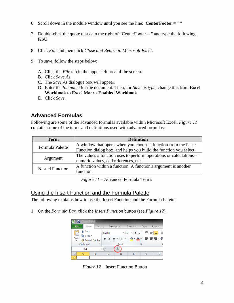
Using the Insert Function and the Formula Palette

The following explains how to use the Insert Function and the Formula Palette:

1. On the Formula Bar, click the Insert Function button (see Figure 12).

Figure 11 – Advanced Formula Terms

Figure 12 – Insert Function Button

10

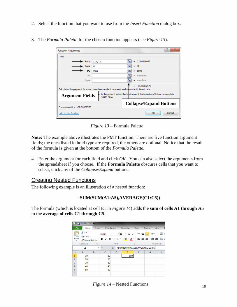
2. Select the function that you want to use from the Insert Function dialog box.

3. The Formula Palette for the chosen function appears (see Figure 13).

Note: The example above illustrates the PMT function. There are five function argument

fields; the ones listed in bold type are required, the others are optional. Notice that the result

of the formula is given at the bottom of the Formula Palette.

4. Enter the argument for each field and click OK. You can also select the arguments from

the spreadsheet if you choose. If the Formula Palette obscures cells that you want to

select, click any of the Collapse/Expand buttons.

Creating Nested Functions

The following example is an illustration of a nested function:

=SUM(SUM(A1:A5),AVERAGE(C1:C5))

The formula (which is located at cell E1 in Figure 14) adds the sum of cells A1 through A5

to the average of cells C1 through C5.

Argument Fields

Argument Fields

Collapse/Expand Buttons

Figure 13 – Formula Palette

Figure 14 – Nested Functions

11

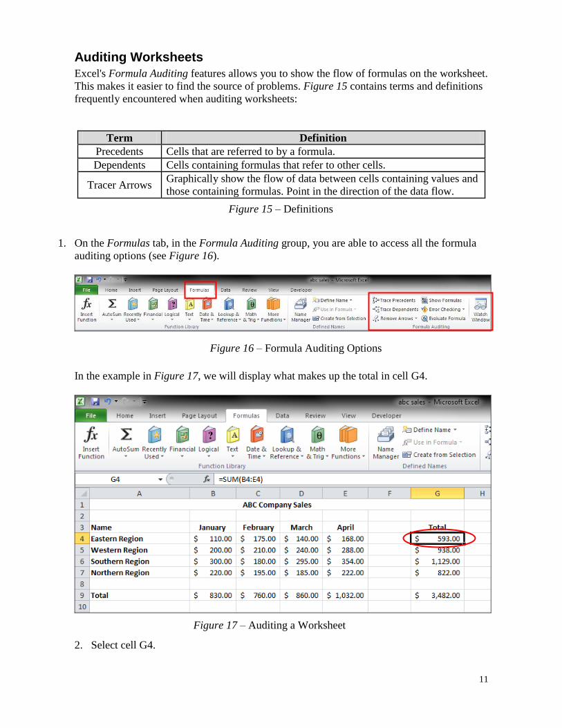
Auditing Worksheets

Excel's Formula Auditing features allows you to show the flow of formulas on the worksheet.

This makes it easier to find the source of problems. Figure 15 contains terms and definitions

frequently encountered when auditing worksheets:

Term Definition

Precedents Cells that are referred to by a formula.

Dependents Cells containing formulas that refer to other cells.

Tracer Arrows Graphically show the flow of data between cells containing values and

those containing formulas. Point in the direction of the data flow.

1. On the Formulas tab, in the Formula Auditing group, you are able to access all the formula

auditing options (see Figure 16).

In the example in Figure 17, we will display what makes up the total in cell G4.

2. Select cell G4.

Figure 15 – Definitions

Figure 16 – Formula Auditing Options

Figure 17 – Auditing a Worksheet

12

3. In the Formula Auditing group, select the Trace Precedents option (see Figure 18).

4. The Trace Arrow indicates that cells B4 through E4 are the cells referred to in the

formula in cell G4 (see Figure 18).

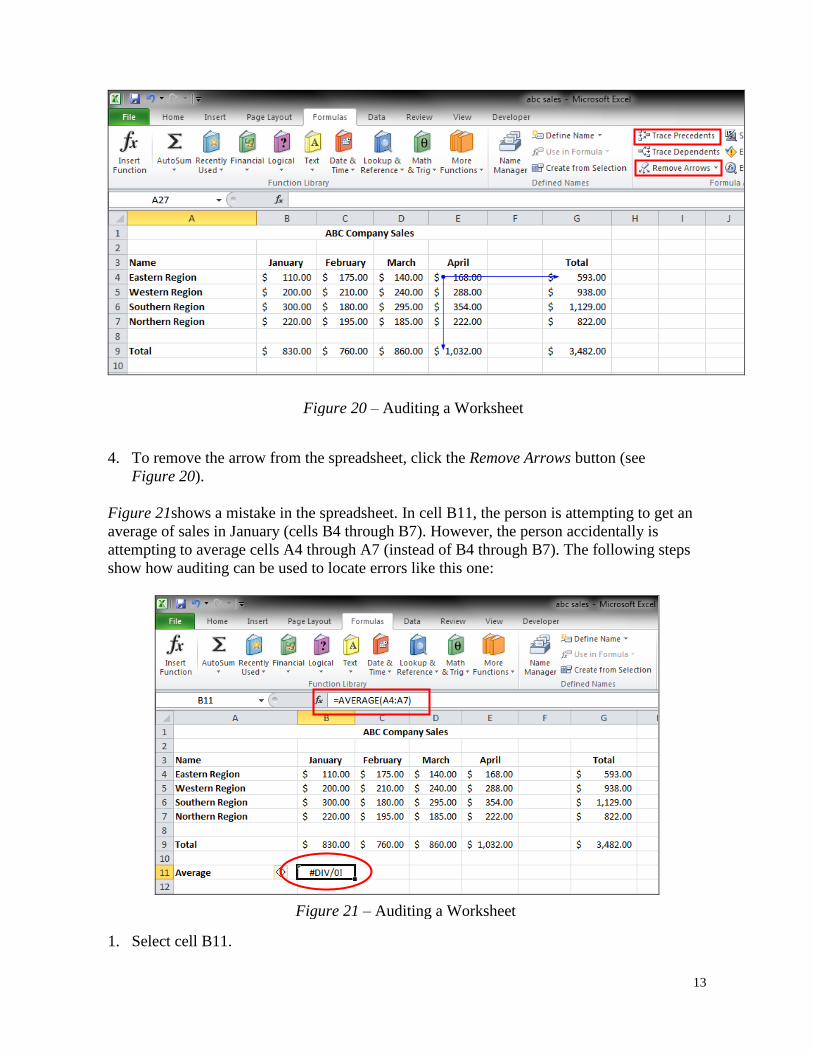
5. To remove the arrow from the spreadsheet, click the Remove Arrows button (see

Figure 18).

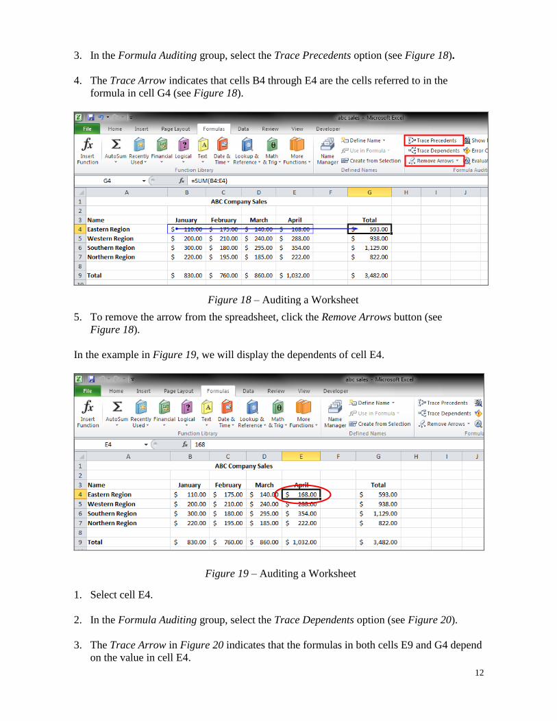
In the example in Figure 19, we will display the dependents of cell E4.

1. Select cell E4.

2. In the Formula Auditing group, select the Trace Dependents option (see Figure 20).

3. The Trace Arrow in Figure 20 indicates that the formulas in both cells E9 and G4 depend

on the value in cell E4.



13


Figure 20).

Figure 21shows a mistake in the spreadsheet. In cell B11, the person is attempting to get an

average of sales in January (cells B4 through B7). However, the person accidentally is

attempting to average cells A4 through A7 (instead of B4 through B7). The following steps

show how auditing can be used to locate errors like this one:

1. Select cell B11.



14

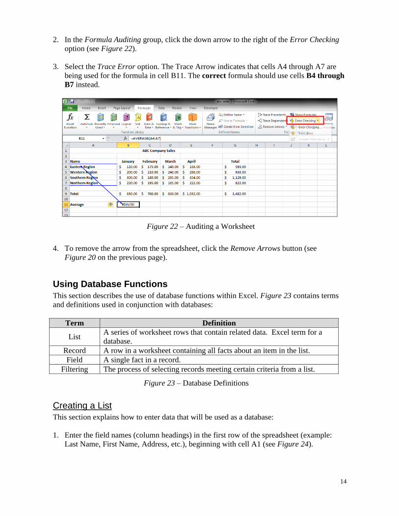
2. In the Formula Auditing group, click the down arrow to the right of the Error Checking

option (see Figure 22).

3. Select the Trace Error option. The Trace Arrow indicates that cells A4 through A7 are

being used for the formula in cell B11. The correct formula should use cells B4 through

B7 instead.


Figure 20 on the previous page).

Using Database Functions

This section describes the use of database functions within Excel. Figure 23 contains terms

and definitions used in conjunction with databases:

Term Definition

List A series of worksheet rows that contain related data. Excel term for a

database.

Record A row in a worksheet containing all facts about an item in the list.

Field A single fact in a record.

Filtering The process of selecting records meeting certain criteria from a list.

Creating a List

This section explains how to enter data that will be used as a database:

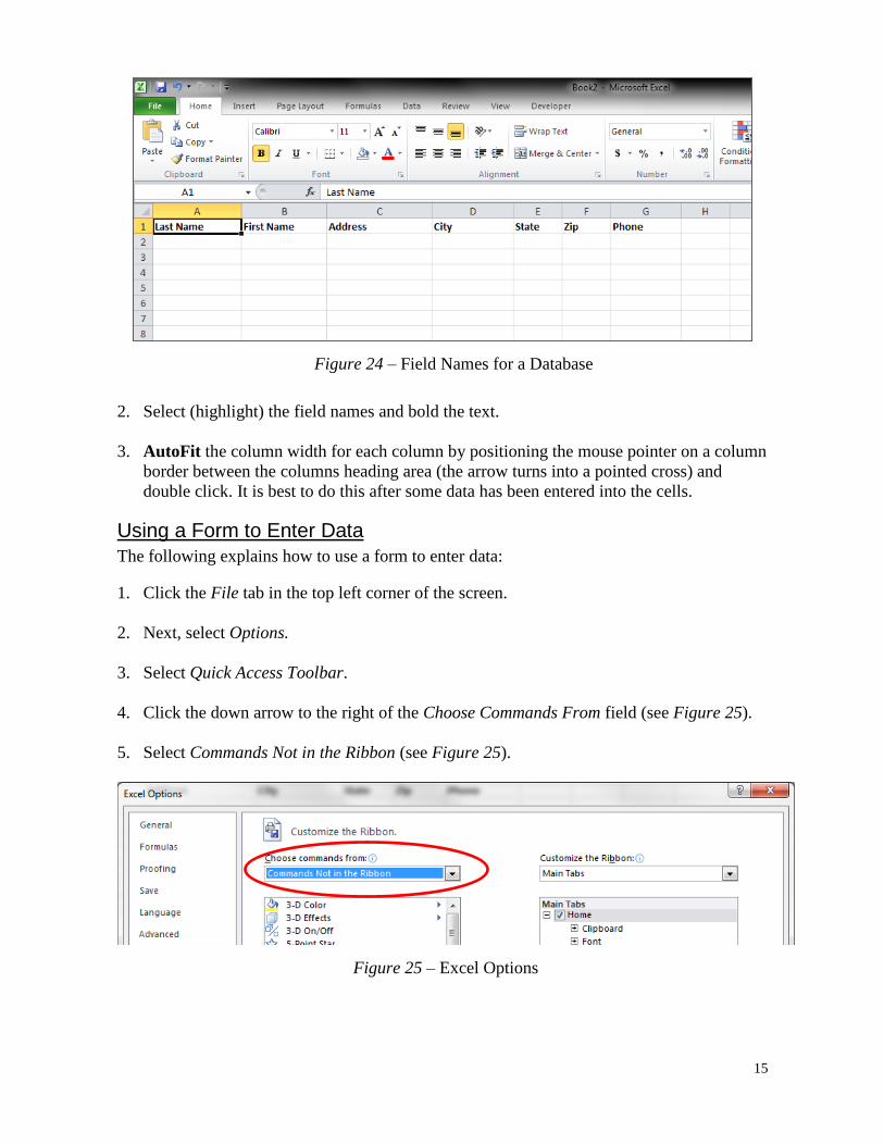
1. Enter the field names (column headings) in the first row of the spreadsheet (example:

Last Name, First Name, Address, etc.), beginning with cell A1 (see Figure 24).


Figure 23 – Database Definitions

15

2. Select (highlight) the field names and bold the text.

3. AutoFit the column width for each column by positioning the mouse pointer on a column

border between the columns heading area (the arrow turns into a pointed cross) and

double click. It is best to do this after some data has been entered into the cells.

Using a Form to Enter Data

The following explains how to use a form to enter data:

1. Click the File tab in the top left corner of the screen.

2. Next, select Options.

3. Select Quick Access Toolbar.

4. Click the down arrow to the right of the Choose Commands From field (see Figure 25).

5. Select Commands Not in the Ribbon (see Figure 25).

Figure 24 – Field Names for a Database


16

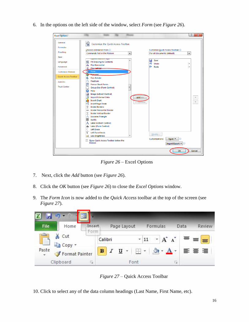
6. In the options on the left side of the window, select Form (see Figure 26).

7. Next, click the Add button (see Figure 26).

8. Click the OK button (see Figure 26) to close the Excel Options window.

9. The Form Icon is now added to the Quick Access toolbar at the top of the screen (see

Figure 27).

10. Click to select any of the data column headings (Last Name, First Name, etc).


Figure 27 – Quick Access Toolbar

17

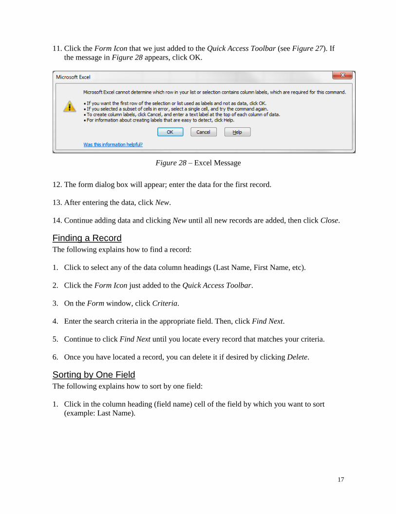
11. Click the Form Icon that we just added to the Quick Access Toolbar (see Figure 27). If

the message in Figure 28 appears, click OK.

12. The form dialog box will appear; enter the data for the first record.

13. After entering the data, click New.

14. Continue adding data and clicking New until all new records are added, then click Close.

Finding a Record

The following explains how to find a record:


2. Click the Form Icon just added to the Quick Access Toolbar.

3. On the Form window, click Criteria.

4. Enter the search criteria in the appropriate field. Then, click Find Next.

5. Continue to click Find Next until you locate every record that matches your criteria.

6. Once you have located a record, you can delete it if desired by clicking Delete.

Sorting by One Field

The following explains how to sort by one field:

1. Click in the column heading (field name) cell of the field by which you want to sort

(example: Last Name).

Figure 28 – Excel Message

18

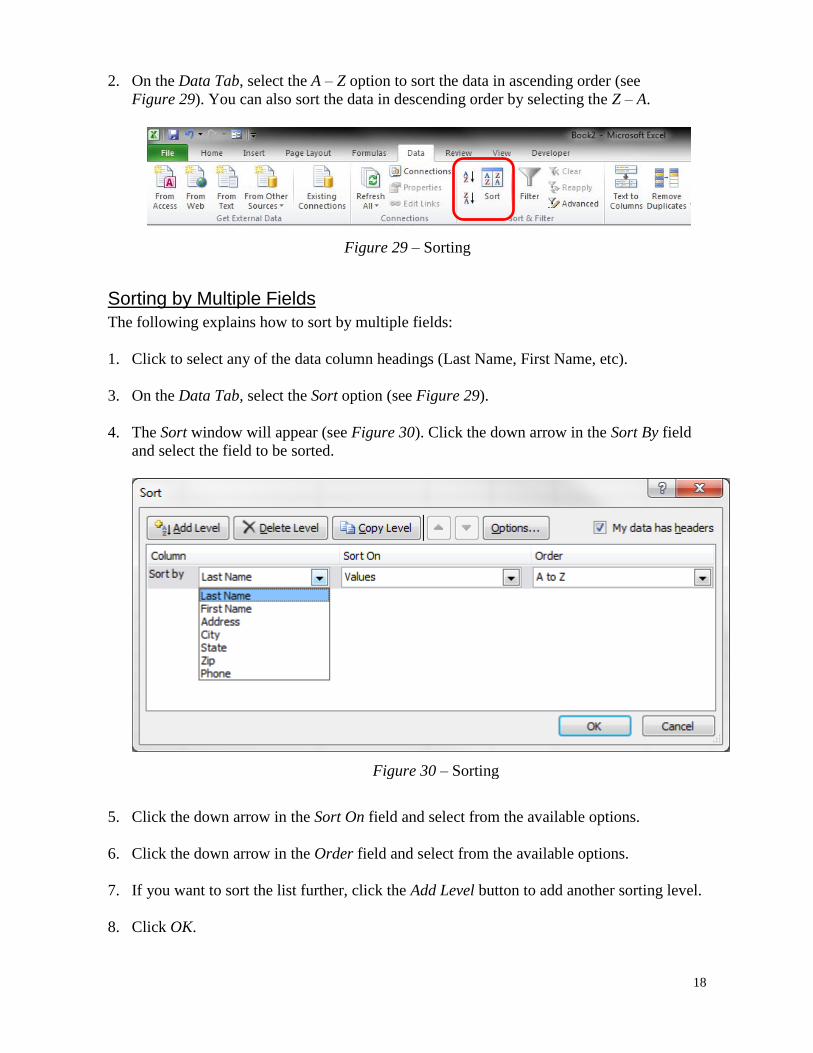
2. On the Data Tab, select the A – Z option to sort the data in ascending order (see

Figure 29). You can also sort the data in descending order by selecting the Z – A.

Sorting by Multiple Fields

The following explains how to sort by multiple fields:


3. On the Data Tab, select the Sort option (see Figure 29).

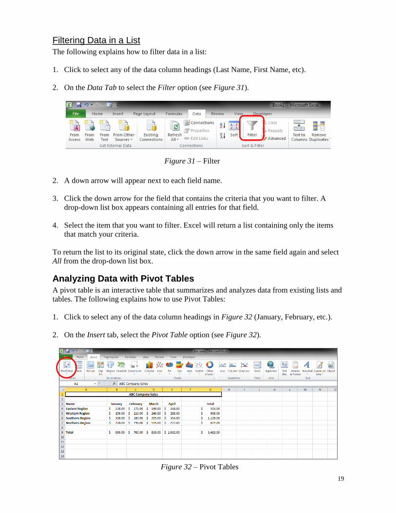
4. The Sort window will appear (see Figure 30). Click the down arrow in the Sort By field

and select the field to be sorted.

5. Click the down arrow in the Sort On field and select from the available options.

6. Click the down arrow in the Order field and select from the available options.

7. If you want to sort the list further, click the Add Level button to add another sorting level.

8. Click OK.

Figure 29 – Sorting

Figure 30 – Sorting

19

Filtering Data in a List

The following explains how to filter data in a list:


2. On the Data Tab to select the Filter option (see Figure 31).

2. A down arrow will appear next to each field name.

3. Click the down arrow for the field that contains the criteria that you want to filter. A

drop-down list box appears containing all entries for that field.

4. Select the item that you want to filter. Excel will return a list containing only the items

that match your criteria.

To return the list to its original state, click the down arrow in the same field again and select

All from the drop-down list box.

Analyzing Data with Pivot Tables

A pivot table is an interactive table that summarizes and analyzes data from existing lists and

tables. The following explains how to use Pivot Tables:

1. Click to select any of the data column headings in Figure 32 (January, February, etc.).

2. On the Insert tab, select the Pivot Table option (see Figure 32).

Figure 31 – Filter

Figure 32 – Pivot Tables

20

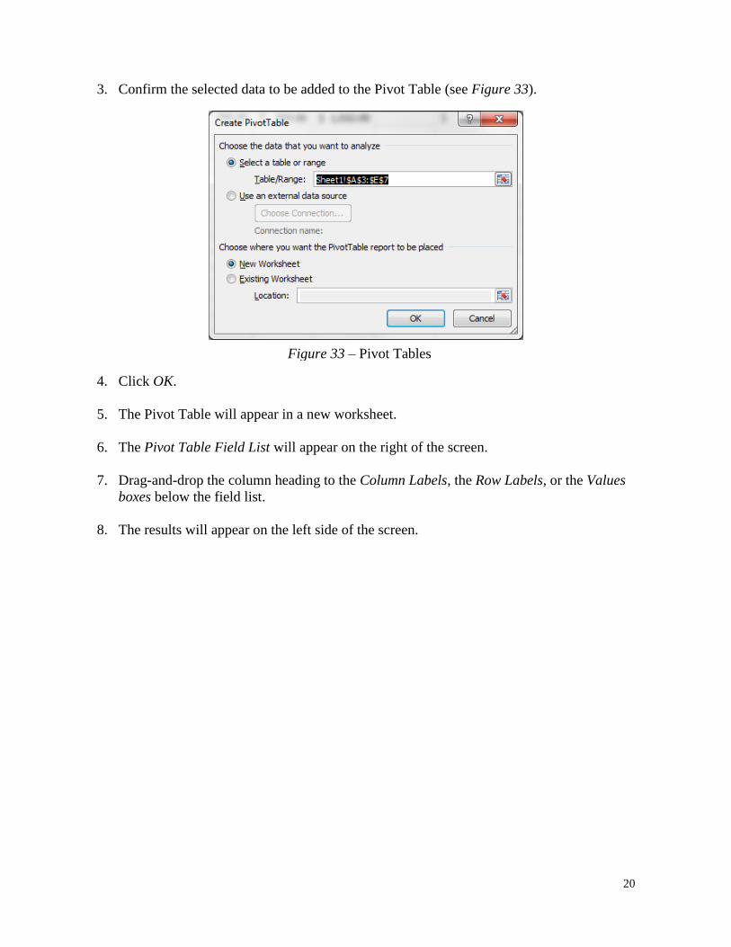
3. Confirm the selected data to be added to the Pivot Table (see Figure 33).

4. Click OK.

5. The Pivot Table will appear in a new worksheet.

6. The Pivot Table Field List will appear on the right of the screen.

7. Drag-and-drop the column heading to the Column Labels, the Row Labels, or the Values

boxes below the field list.

8. The results will appear on the left side of the screen.

Figure 33 – Pivot Tables

21

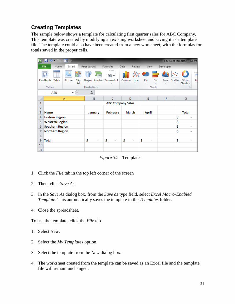
Creating Templates

The sample below shows a template for calculating first quarter sales for ABC Company.

This template was created by modifying an existing worksheet and saving it as a template

file. The template could also have been created from a new worksheet, with the formulas for

totals saved in the proper cells.

1. Click the File tab in the top left corner of the screen

2. Then, click Save As.

3. In the Save As dialog box, from the Save as type field, select Excel Macro-Enabled

Template. This automatically saves the template in the Templates folder.

4. Close the spreadsheet.

To use the template, click the File tab.

1. Select New.

2. Select the My Templates option.

3. Select the template from the New dialog box.

4. The worksheet created from the template can be saved as an Excel file and the template

file will remain unchanged.

Figure 34 – Templates

22

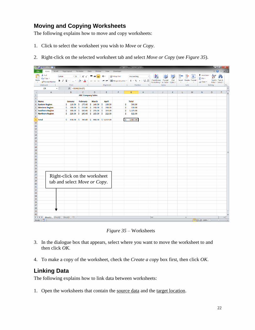
Moving and Copying Worksheets

The following explains how to move and copy worksheets:

1. Click to select the worksheet you wish to Move or Copy.

2. Right-click on the selected worksheet tab and select Move or Copy (see Figure 35).

3. In the dialogue box that appears, select where you want to move the worksheet to and

then click OK.

4. To make a copy of the worksheet, check the Create a copy box first, then click OK.

Linking Data

The following explains how to link data between worksheets:

1. Open the worksheets that contain the source data and the target location.

Figure 35 – Worksheets

Right-click on the worksheet

tab and select Move or Copy.

23

2. Select the cell(s) in the source worksheet that contain the data that you want to link to the

target location.

3. On the Home tab, select Copy.

4. Go to the target location and select the cell(s) where you want to put the source data.

5. From the Home tab, click the arrow under Paste. Then, select Paste Special at the bottom

of the menu.

6. In the Paste Special dialog box, click the Paste Link button.

7. Click Ok.

The target location will now be updated whenever the source data is changed.

Adding a Comment to a Cell

The following explains how to add a comment to a cell:

1. Select the cell where you want to add the comment.

2. On the Review tab, select New Comment.

3. Type your comment in the comment box that appears. Click outside the comment box

when done.

4. The commented cell is now indicated by a red triangle in the top right corner of the cell.

5. When the mouse pointer is placed over the cell, the comment box appears.

24

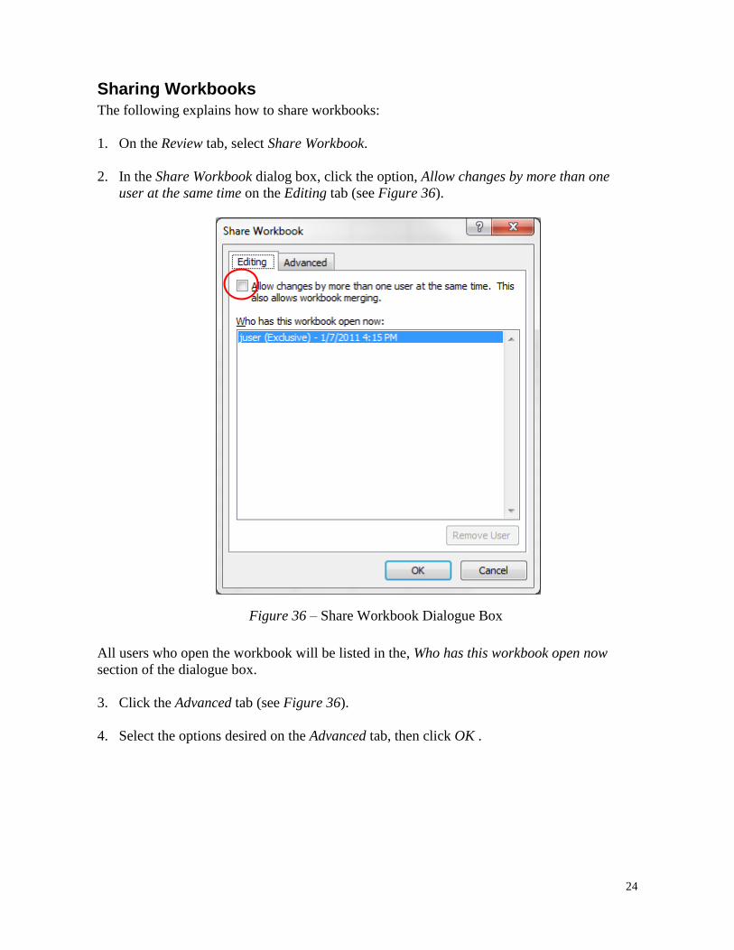
Sharing Workbooks

The following explains how to share workbooks:

1. On the Review tab, select Share Workbook.

2. In the Share Workbook dialog box, click the option, Allow changes by more than one

user at the same time on the Editing tab (see Figure 36).

All users who open the workbook will be listed in the, Who has this workbook open now

section of the dialogue box.

3. Click the Advanced tab (see Figure 36).

4. Select the options desired on the Advanced tab, then click OK .

Figure 36 – Share Workbook Dialogue Box

25

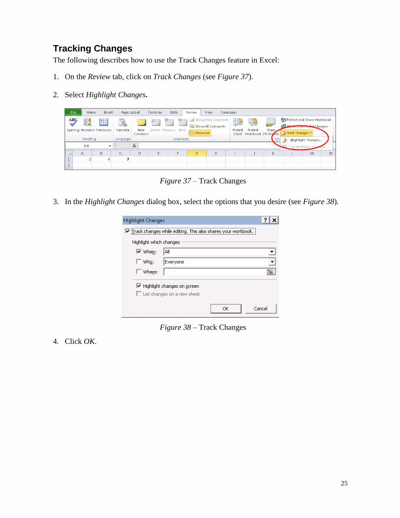
Tracking Changes

The following describes how to use the Track Changes feature in Excel:

1. On the Review tab, click on Track Changes (see Figure 37).

2. Select Highlight Changes.

3. In the Highlight Changes dialog box, select the options that you desire (see Figure 38).

4. Click OK.

Figure 37 – Track Changes


26

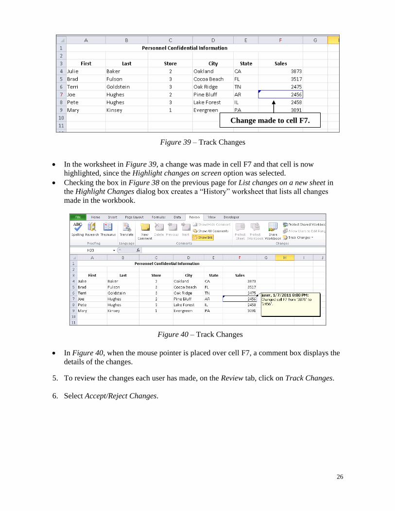
In the worksheet in Figure 39, a change was made in cell F7 and that cell is now

highlighted, since the Highlight changes on screen option was selected.

Checking the box in Figure 38 on the previous page for List changes on a new sheet in

the Highlight Changes dialog box creates a “History” worksheet that lists all changes

made in the workbook.

In Figure 40, when the mouse pointer is placed over cell F7, a comment box displays the

details of the changes.

5. To review the changes each user has made, on the Review tab, click on Track Changes.

6. Select Accept/Reject Changes.

Change made to cell F7.



27

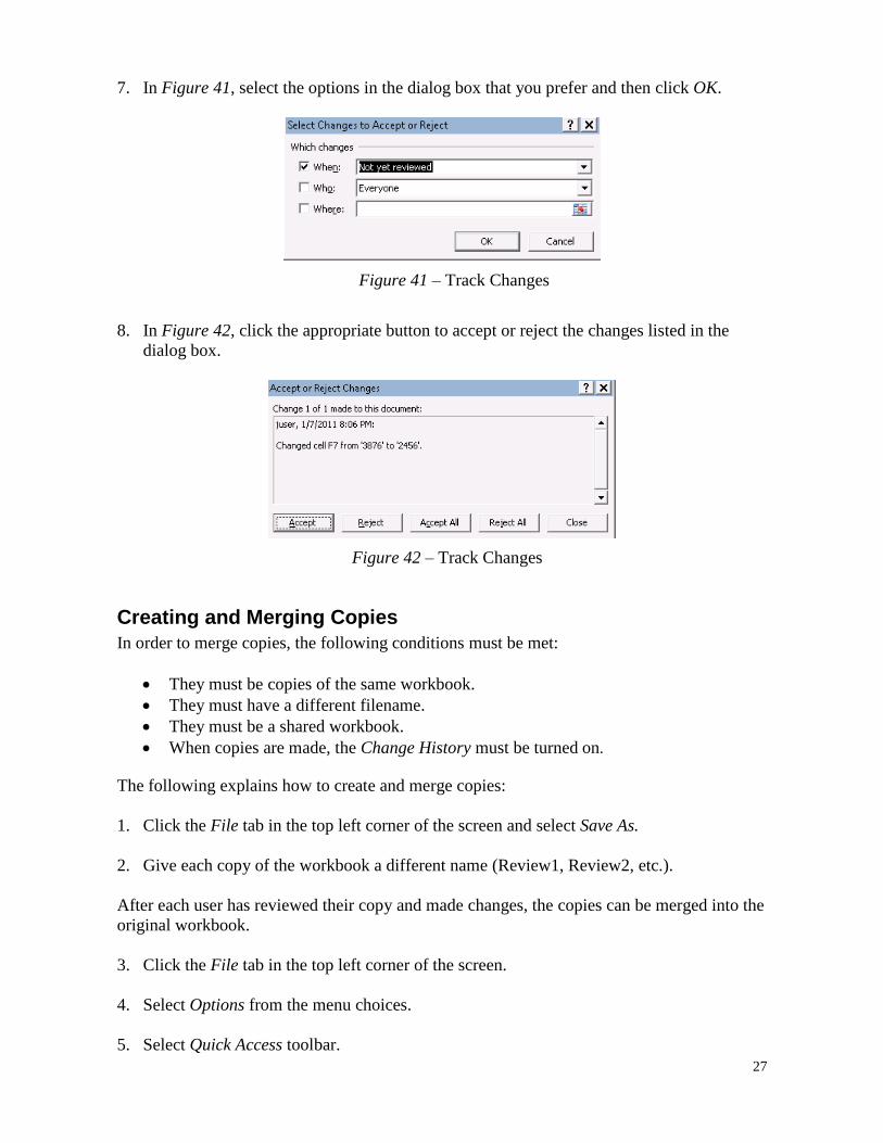
7. In Figure 41, select the options in the dialog box that you prefer and then click OK.

8. In Figure 42, click the appropriate button to accept or reject the changes listed in the

dialog box.

Creating and Merging Copies

In order to merge copies, the following conditions must be met:

They must be copies of the same workbook.

They must have a different filename.

They must be a shared workbook.

When copies are made, the Change History must be turned on.

The following explains how to create and merge copies:

1. Click the File tab in the top left corner of the screen and select Save As.

2. Give each copy of the workbook a different name (Review1, Review2, etc.).

After each user has reviewed their copy and made changes, the copies can be merged into the

original workbook.


4. Select Options from the menu choices.

5. Select Quick Access toolbar.



28

6. In the Choose commands from list, select All Commands.

7. Select Compare and Merge Workbooks. Then, click the Add button.

8. Click OK.

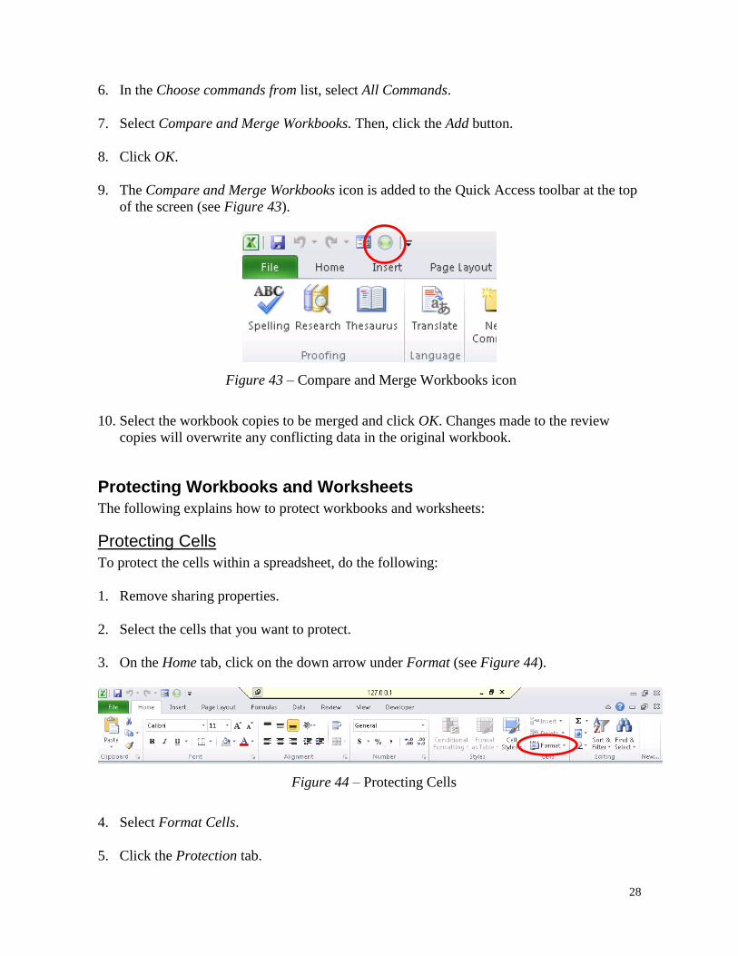
9. The Compare and Merge Workbooks icon is added to the Quick Access toolbar at the top

of the screen (see Figure 43).

10. Select the workbook copies to be merged and click OK. Changes made to the review

copies will overwrite any conflicting data in the original workbook.

Protecting Workbooks and Worksheets

The following explains how to protect workbooks and worksheets:

Protecting Cells

To protect the cells within a spreadsheet, do the following:

1. Remove sharing properties.

2. Select the cells that you want to protect.

3. On the Home tab, click on the down arrow under Format (see Figure 44).

4. Select Format Cells.

5. Click the Protection tab.

Figure 43 – Compare and Merge Workbooks icon

Figure 44 – Protecting Cells

29

6. Click to place a check by the Locked checkbox to prevent changes to cells.

7. Click to place a check by the Hidden checkbox to prevent formulas from being seen by

other users.

8. Click OK to close the dialog box.

NOTE: Locking or hiding has no effect unless the worksheet is protected.

To hide rows, columns, or sheets, do the following:

1. From the Home tab, click Format.

2. Select Hide & Unhide.

3. Select either Row, Column, or Sheet.

Protecting Worksheets

The following explains how to protect worksheets:

1. On the Home tab, click the down arrow under Format.

2. Select Protect Sheet.

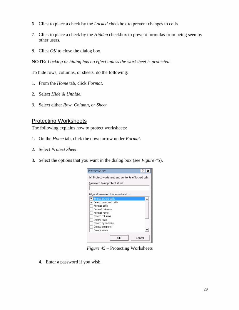
3. Select the options that you want in the dialog box (see Figure 45).

4. Enter a password if you wish.

Figure 45 – Protecting Worksheets

30

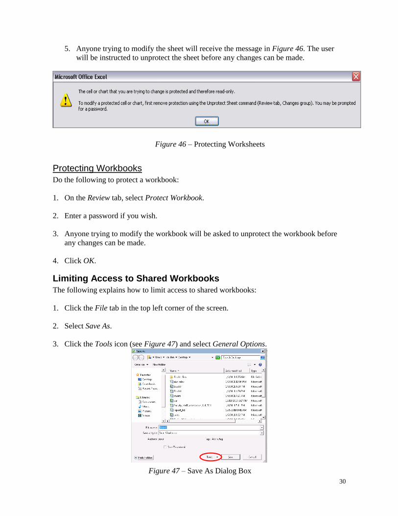
5. Anyone trying to modify the sheet will receive the message in Figure 46. The user

will be instructed to unprotect the sheet before any changes can be made.

Protecting Workbooks

Do the following to protect a workbook:

1. On the Review tab, select Protect Workbook.

2. Enter a password if you wish.

3. Anyone trying to modify the workbook will be asked to unprotect the workbook before

any changes can be made.

4. Click OK.

Limiting Access to Shared Workbooks

The following explains how to limit access to shared workbooks:


2. Select Save As.

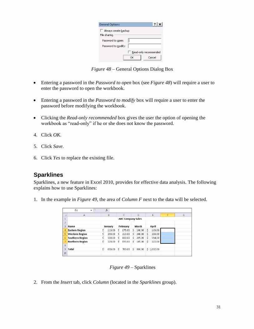
3. Click the Tools icon (see Figure 47) and select General Options.

Figure 46 – Protecting Worksheets

Figure 47 – Save As Dialog Box

31

Entering a password in the Password to open box (see Figure 48) will require a user to

enter the password to open the workbook.

Entering a password in the Password to modify box will require a user to enter the

password before modifying the workbook.

Clicking the Read-only recommended box gives the user the option of opening the

workbook as “read-only” if he or she does not know the password.

4. Click OK.

5. Click Save.

6. Click Yes to replace the existing file.

Sparklines

Sparklines, a new feature in Excel 2010, provides for effective data analysis. The following

explains how to use Sparklines:

1. In the example in Figure 49, the area of Column F next to the data will be selected.

2. From the Insert tab, click Column (located in the Sparklines group).

Figure 48 – General Options Dialog Box

Figure 49 – Sparklines

32

3. The Create Sparklines dialogue box will appear (see Figure 50). Enter the data range in

the first text box. For the example in Figure 49, we would enter the following range:

B4:E7

4. Click OK. The charts will appear in Column F, allowing you to visually analyze your

data (see Figure 51).

Slicer

The new Slicer feature in Excel 2010 helps users to break down data in Pivot Tables that

would otherwise be very overwhelming. The following steps describe how to use the Slicer

feature:

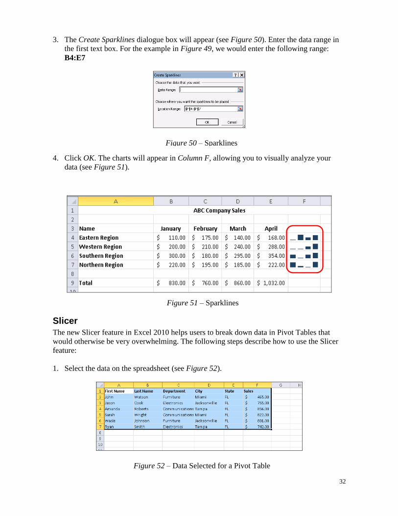
1. Select the data on the spreadsheet (see Figure 52).



Figure 52 – Data Selected for a Pivot Table

33

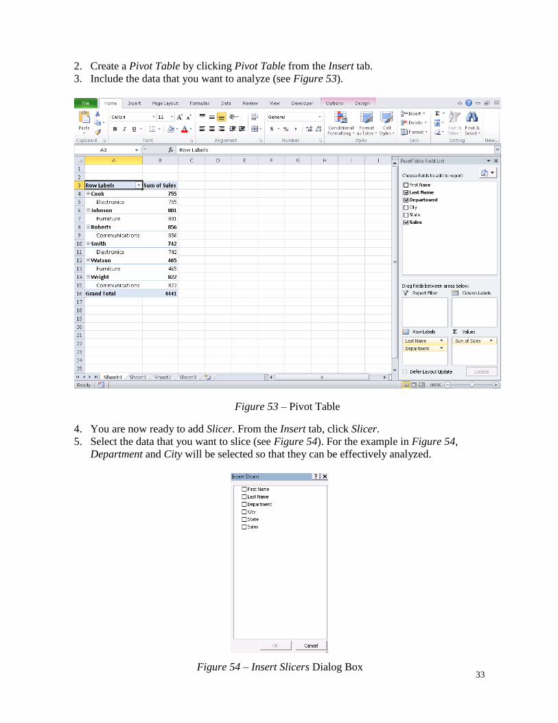
2. Create a Pivot Table by clicking Pivot Table from the Insert tab.

3. Include the data that you want to analyze (see Figure 53).

4. You are now ready to add Slicer. From the Insert tab, click Slicer.

5. Select the data that you want to slice (see Figure 54). For the example in Figure 54,

Department and City will be selected so that they can be effectively analyzed.

Figure 53 – Pivot Table

Figure 54 – Insert Slicers Dialog Box

34

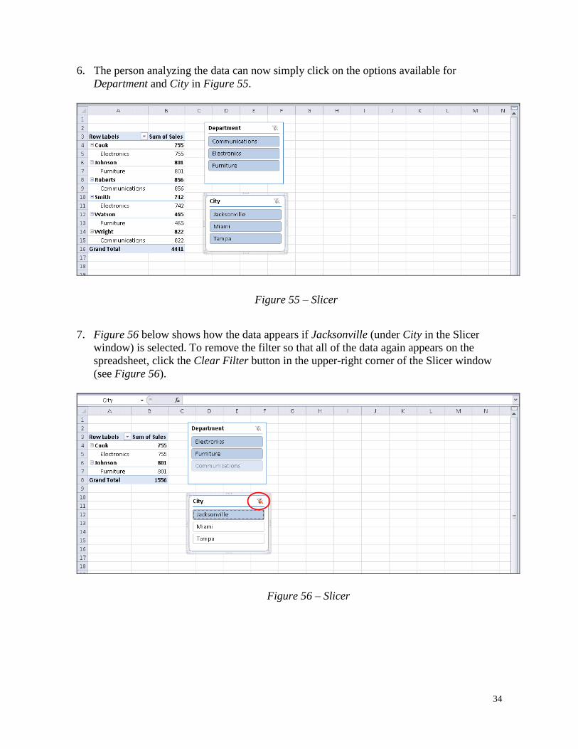
6. The person analyzing the data can now simply click on the options available for

Department and City in Figure 55.

7. Figure 56 below shows how the data appears if Jacksonville (under City in the Slicer

window) is selected. To remove the filter so that all of the data again appears on the

spreadsheet, click the Clear Filter button in the upper-right corner of the Slicer window

(see Figure 56).

Figure 55 – Slicer

Figure 56 – Slicer

microsoft excel 2010 - kennesaw state university excel 2010 ... excel's formula auditing...

Documents