Microeconomics of Banking

Spring trimester, 2011 at the Toulouse School of Economics

These notes have been compiled in the hope they may serve as a useful studyaid for students in the Microeconomics of Banking course at TSE. Greatfulthanks to Nicolas who composed the �rst portion of this document, and withwhom I have collaborated on this project. My grateful appreciation to professorPlantin, whose lectures are the basis for these notes, and for making his slidesavailable. I would be glad to hear any comments or suggestions for improvementthat may occur to the reader. All errors remain my own. - MJM

1

Contents

Contents 20.1 Course Information . . . . . . . . . . . . . . . . . . . . . . . . . 40.2 Introduction . . . . . . . . . . . . . . . . . . . . . . . . . . . . . 4

0.2.1 Functions of Banks: . . . . . . . . . . . . . . . . . . . . 60.2.1.1 O�ering liquidity and payment services . . . . 60.2.1.2 Transforming assets . . . . . . . . . . . . . . . 70.2.1.3 Managing Risk . . . . . . . . . . . . . . . . . . 70.2.1.4 Monitoring and Information Processing . . . . 8

0.2.2 Resource allocation . . . . . . . . . . . . . . . . . . . . . 90.2.3 Banking in the Arrow-Debreu Model . . . . . . . . . . . 10

I The Role of Financial Intermediaries (FIs) 130.3 Introduction . . . . . . . . . . . . . . . . . . . . . . . . . . . . . 140.4 Diamond and Dybvig . . . . . . . . . . . . . . . . . . . . . . . . 160.5 Leland and Pyle . . . . . . . . . . . . . . . . . . . . . . . . . . 20

0.5.1 Model of Capital Market with Adverse Selection . . . . 200.5.2 Signalling . . . . . . . . . . . . . . . . . . . . . . . . . . 220.5.3 Coalition of Borrowers . . . . . . . . . . . . . . . . . . . 23

0.6 Diamond (1984) . . . . . . . . . . . . . . . . . . . . . . . . . . 230.6.1 Delegated Monitoring Theory . . . . . . . . . . . . . . . 230.6.2 Model: . . . . . . . . . . . . . . . . . . . . . . . . . . . . 24

0.7 Banks Loans vs. Direct Debts . . . . . . . . . . . . . . . . . . . 270.7.1 Introduction . . . . . . . . . . . . . . . . . . . . . . . . 270.7.2 Model of Credit Market with Moral Hazard . . . . . . . 270.7.3 Reputation . . . . . . . . . . . . . . . . . . . . . . . . . 29

0.7.3.1 Diamond (1991) . . . . . . . . . . . . . . . . . 290.7.3.2 Financial Capital - Holmstrom and Tirole (1997) 310.7.3.3 Bank Loans vs. Direct Debt - Bolton and Frex-

ias (2000) . . . . . . . . . . . . . . . . . . . . . 36

II The Industrial Organization Approach 400.8 Introduction . . . . . . . . . . . . . . . . . . . . . . . . . . . . . 41

2

CONTENTS 3

0.9 Perfect Competitive Banks . . . . . . . . . . . . . . . . . . . . 410.9.1 Financial Sector . . . . . . . . . . . . . . . . . . . . . . 410.9.2 Interaction with the real sector . . . . . . . . . . . . . . 410.9.3 Credit Multiplier Approach . . . . . . . . . . . . . . . . 420.9.4 Monopolistic Bank (Monti-Klein Model) . . . . . . . . . 45

0.9.4.1 Model . . . . . . . . . . . . . . . . . . . . . . . 460.9.5 The Threat of Termination (Bolton and Scharfstein, 1990) 460.9.6 Judicial Enforcement (Japelli, Pagano, and Bianco, 2005) 480.9.7 Securitization . . . . . . . . . . . . . . . . . . . . . . . . 54

CONTENTS 4

0.1 Course Information

Texbook: Freixas, X. and J.C. Rochet "Microeconomics of Banking", MITPress, second edition

Professor: Guillaume Plantin.

guillaume.plantin@tse-fr.eu

Tél.: +33 (0)5 61 12 86 01

Bureau: MF 306

Secrétaire: Aline Soulie

Courriel: aline.soulie@tse-fr.eu, Tél. : +33 (0)5 61 12 85 56, Bureau : MF218

Exam: The professor provided a few comments about the exam halfwaythrough the lectures, saying it would be a two hour closed bookexamination. Though he hadn't composed it at the date of hiscomments, he stated it would possibly contain one essay type ques-tion, to check that we can make use of the models we studied inclass to make arguments, and an additional one or two problemsregarding the type of models we saw in class

0.2 Introduction

De�nition. (Bank) a Bank is an institution whose current operations consistin granting loans and receiving deposits from the public. Let's break down thisde�ntion, to be as precise as possible.

• "Current": current operations vs. occasional operations

• "And": combination of lending and borrowing is typical characteristicsof commercial banks

• "Public": on the liabilities side of the bank, the customers are generalpublic which is not armed to assess the safety and soundness of �nan-cial institutions. The following schematic shows the components of theeconomy we consider in our models:

CONTENTS 5

In studying the microeconomics of banking, we shall make a distinctionbetween two sources of demand for funds. Broadly, it is possible to distinguish'banks' from 'markets' as places which attract the funds supplied by households.

First a word about markets - these can be further seperated into central-ized and decentralized markets. Most markets attracting funds from lenders,savers or the general public are decentralized. Decentralized markets or over-the-counter (OTC) markets include most derivatives markets, corporate bondmarkets, and the foreign exchange (Forex) market, while centralized marketsinclude most stock markets and some derivatives markets like Chicago Mercan-tile Exchange. Our discussion will begin however, with banks, of which thereare two main types we study:

• Commercial banks

� These issue loans which are non-contigent on a speci�c project (asopposed to equity); they typically are large and long-term assets.From the bank's point of view (and as re�ected on their balancesheet), these loans are assets whose cash�ows are the payment streamsof interest and principal associated to them.

� The bank's liabilities are the deposits of their customers. Depositsare contracts where the depositors lend money to the bank, butwith a liquidity option which allows them to withdraw money easily.They are typically small (relative to loans), and unlike the loansbanks make, which tend to have a well-speci�ed set of repaymenttimes, the liquidity feature means that they bank needs to be readyto repay depositors the money they've lent at any time.

∗ Thus, there is a discrepancy between the terms of the contracts,which means the bank has risk.

CONTENTS 6

∗ Some (ex. Friedman) voice the opinion that this discrepancy isan historical accident.

∗ Note: It could be quite costly for a single, small depositor tomonitor the solvency of the bank where they make their deposit,and would cause free-riding problems if some, but not all, peoplewere monitoring.

• Investment banks

� Advise �rms issuing bonds and equity

� Advise banks wishing to securitize a portfolio of loans

� Generally, help people to gain access to the �nancial markets. Forexample, they could supervise, for insurance reasons, and monitor a�rm wishing to make an IPO

0.2.1 Functions of Banks:

1. O�ering liquidity and payment services (this includes automatic tellermachines, providing checkbooks, etc.)

2. Transforming assets

a) Convenience of denomination (amount)

b) Quality transformation

c) Maturity (duration) transformation

3. Managing risks

a) Credit risk

b) Interest rate and liquidity risk

4. Processing information and monitoring borrowers

0.2.1.1 O�ering liquidity and payment services

• Here, a slight historical detour. In the past, banks played two di�erentparts in the management of �at money: money changing and provisionof payment services

� Money changing

∗ Greece: Trapeza (Greek word for bank): means 'balance' thatwas used by early money changers to weigh coins

∗ Italy: Banco (Italian word for bank): bench on which the moneychangers placed their precious coins

∗ Management of deposits

CONTENTS 7

· Safekeeping services: initially, bank deposits were not sup-posed to be lent and they had a zero (or even negative, tocompensate the bank for their expenses) return

· Convertible into "good money": Coins di�ered in their com-position of precious metals and banks are required to makepayment in good money

∗ Payment services

· They cover both the management of clients' accounts andthe �nality of payments

· The safety and e�ciency of these payment systems havebecome a fundamental concern for governments and centralbanks

0.2.1.2 Transforming assets

• Convenience of denomination

� Banks choose the unit size (denomination) of its products (depositsand loans) in a way that is convenient for its clients

∗ Typically collect small deposits and invest the proceeds intolarge loans

� Quality transformation

∗ Bank deposits o�er better risk-return characteristics than directinvestments. Reasons:

· Indivisibilities in the investment: small investors cannot di-versify their portfolio

· Asymmetric information: banks have better informationthan depositors about the entrepreneurs and �rms they �-nance

� Maturity transformation

∗ Transforming securities with short maturities into securities withlong maturities (accepting deposits and making loans)

∗ Origin of interest rate and liquidity risks

0.2.1.3 Managing Risk

• Credit risk

� That is the risk that a borrower is not able to repay a debt (principalor interest)

∗ Banks tried to make their loans secure either through collateral,through the assignment of rights or through the endorsement bya city

CONTENTS 8

∗ Commercial bank are doing tranching, which means they takethe �rst losses. When losses occur, it is sustain by the capi-tal and, when there is no capital remaining, it then a�ects theavailability of deposits.

� Interest rate and Liquidity risks

∗ Maturity transformation exposes banks to risks

· Cost of funds (which depends on the level of short-terminterest rates) may rise above the contractual interest ratesof the loans granted by the banks

· Unexpected withdrawals of deposits may force banks to seekmore expensive sources of funds

� =⇒ Banks have to manage the combination of interest rate risk (dueto the di�erence in maturity) and liquidity risk (due to the di�erencein the marketability of the claims issued and of the claims held)

� The internal rate of return a bank ask on her loans should be linkedto the weighted cost of capital from deposits and equity.

0.2.1.4 Monitoring and Information Processing

• Banks screen loan applicants and monitor the way the businesses they�nance manage their projects. Through these activities, banks and theirborrowers develop long-term relationships, thus mitigating the e�ects ofmoral hazard

� This is one of main di�erences between bank lending and issuingsecurities in the �nancial markets. One way of thinking about thevalue of a bank loan, over and above direct lending, is that whichresults from the long-term relationship =⇒ we can also note thatthe loan value is a priori unknown to outsiders: bank loans are"opaque"

• Securitization may induce some problems, since the bank may not havethe incentive to maintain their role of monitoring loans. They createshort-term instruments and sell them, hence the long-term relationshipis further transformed in a short-term one.

CONTENTS 9

• U.S. relies more on stock markets and the Euro area relies more on thebanking system

0.2.2 Resource allocation

Some general comments on how banks play a role in the way resources areallocated in an economy. Banks exert a fundamental in�uence on capital allo-cation, risk sharing and economic growth

• Underdeveloped economies with a low level of �nancial intermediationand small, illiquid �nancial markets may be unable to channel savingse�ciently

• Market-oriented economies are not very good at dealing with nondiversi-�able risks

CONTENTS 10

• Banks' reserves function as a bu�er against macroeconomic shocks andallow for better intertemporal risk sharing

• Bank-oriented economies are not very good at �nancing new technologies.Markets are much better for dealing with di�erences of opinion amonginvestors about these new technologies

• Market-oriented economies are better at innovating, since there are morepeople looking at the innovating sectors and o�ering opinion, hence theinformation is more accurate.

0.2.3 Banking in the Arrow-Debreu Model

• The economy:

� Two dates: t = 1; 2

� Unique physical good initially owned by consumers

� Agents are households (h), �rms (f), and banks (b). All agentsbehave competitively.

• Consumers:

� Choose date 1 and 2 consumption (C1, C2) and the allocation ofsavings, which is split between a deposit D in a bank and bonds B

CONTENTS 11

held in the market for �rm debt (Dh, Bh) such thatmaxU(C1, C2)

s.t.

{C1 +Dh +Bh = ω1

ρC2 = Πf + Πb + (1 + r)Bh + (1 + rD)Dh,

where ρ is the level of in�ation, r is the time 2 return o�ered bybanks to investing 1 unit of currency in time 1, Dh is the amount ofdeposit made by the household and Bh is the amount in bonds heldby the household. In words, the above says that consumers maximizetheir total utility from period one and period 2 such that all theirinitial wealth at time 1 is split between consumption, bank deposits,and lending to the bond market, and that their consumption at time2 equals their in�ation-adjusted payments from their ownership of�rms and banks plus the repayment of the principal and interest ontheir bonds plus the principal and interest on their bank deposits.

� Interior solution: r = rD; if there is no friction this condition isrequired for the market to clear

• Firms choose investment level I and its �nancing from bank loans L andbonds B, (Lf , Bf ) such that they maximize their pro�ts

max Πf

s.t.

{Πf = pf(I)− (1 + r)Bf − (1 + rL)Lf ,

I = Bf + Lf

which yields an interior solution: r = rL by market clearing condition.

• Banks choose loan supply Lb and its �nancing (Db, Bb) to maximize theirpro�ts

max Πb

s.t.

{Πb = rLLb − rBb − rDDb

Lb = Bb +Db

• General equilibrium is characterized by a vector of interest rates (r, rL, rD)and three vectors of demand and supply levels: (C1, C2, Bh, Dh) for theconsumer, (I,Bf , Lf ) for the �rm and (Lb, Bb, Db) for the bank such that

� Each agent behaves optimally, and

� Each market clears:

∗ I = S (goods market)

∗ Db = Dh (deposit market)

∗ Lf = Lb (loan market)

∗ Bh = Bf +Bb (bond market)

CONTENTS 12

Proposition. If �rms and households have unrestricted access to perfect�nancial markets, then in a competitive equilibrium:

Banks make zero pro�t

The size and composition of banks' balance sheets have no e�ect on othereconomic agents

� The markets clear with r = rD = rL

Part I

The Role of FinancialIntermediaries (FIs)

13

CONTENTS 14

0.3 Introduction

De�nition. a Financial Intermediary (FI) is an economic agent who specializesin the activities of buying and selling (at the same time) �nancial claims. Wewill usually generically refer to �nancial intermediaries as 'banks' for modelingpurposes.

• Banks usually deal with �nancial contracts (loans and deposits) whichcannot be easily be resold (are less liquid), as opposed to �nancial secu-rities (stocks and bonds) that are marketable instruments.

� Securitization allows banks to resell the loans they originated. How-ever, asymmetric information may limit the possibilities of securiti-zation

� Banks have to transform �nancial contracts and securities becausethe contracts and securities issued by �rms (borrowers) are usuallydi�erent from those desired by investors (depositors); di�erence induration and size. In addition we have seen in the course on Cor-porate Finance that the less-marketable contracts o�ered by bankstend to have features such as covenants that may require the lenderto maintain a relationship with the borrower, for monitoring pur-poses, for example. If debtholders are broadly dispersed, these kindof contracts will be hard to enforce because of free-rider problems,etc.

• Existence of �nancial institutions:

� Classical transaction cost justi�cations

∗ Existence of economies of scale and economies of scope

∗ Physical and technological costs do not provide a satisfactoryjusti�cation given signi�cant progress in telecommunicationsand computers which we might have expect to have radicallylowered such costs.

� Informational Asymmetries

∗ These asymmetries generate market imperfections that can beseen as speci�c forms of transaction costs

· Banks gather information by accepting deposits and makingloans, hence they have more information on the liquidityprovision; they have more information on risk.

• Classical Theory:

� Do economies of scope exist between deposit and credit activities?

∗ "Central place" story

CONTENTS 15

· Because of transportation costs, it is e�cient for the same�rm or branch to o�er deposit and credit services in a singlelocation

∗ Portfolio theory

· In equilibrium, less risk-averse investors short-sell (borrow)the riskless asset and invest more than their own wealth inthe risky market portfolio

· Diversi�cation argument (Pyle 1971): Banks are interpretedas investors who hold a long position in securities havinga positive expected excess return and a short position insecurities that have a negative expected excess return underthe assumption that the returns of these two categories ofsecurities are positively correlated.

• Pyle:

� The agent (Bank) have mean-variance preferences de�ned by : E[R]−V(R)

� Let's have 3 assets:

return variance

Risk-free r 0Deposit rD σ2

D

Loan rL σ2L

• the correlation between (the return on?) deposits and loans being ρ

• Let ωD and ωL be the proportions of an agent's total wealth ωof depositsand loans respectively. The returns are given by

R = (ω − ωD − ωL) · r + ωD rD + ωLrL,

E[R] = (ω − ωD − ωL) · r + ωDrD + ωLrL

in expectation, and the variance is

V(R) = ω2Dσ

2D + ω2

Lσ2L + 2ρωDωLσDσL.

� The utility function (using the form of mean-variance preferencesstated above) can then be written as :

U = ωD(rD − r) + ωL(rL − r)− ω2Dσ

2D − ω2

Lσ2L − 2ρωDωLσDσL

Maximizing this expression with respect to the share of wealth in-vested in deposits and loans, the �rst order conditions (F.O.C.s)are

∂U

∂ωD= 0 =⇒ rD − r = 2ωDσ

2D + 2ρωLσDσL,

CONTENTS 16

∂U

∂ωL= 0 =⇒ rL − r = 2ωLσ

2L + 2ρωDσDσL,

which is a system of two equations in two unknowns[2σ2

D 2ρσDσL2ρσDσL 2σ2

L

] [ωDωL

]=

[rD − rrL − r

]yielding:

ωD =2(rD − r)σ2

L − 2(rL − r)ρσDσL4σ2

Dσ2L(1− ρ2)

ωL =2(rL − r)σ2

D − 2(rD − r)ρσDσL4σ2

Dσ2L(1− ρ2)

If rD < r < rL and ρ ≥ 0, then we have ωD < 0 and ωL ≥ 0

� The di�culty is to show how to get rD < r < rL and ρ ≥ 0, thetheory does not explain where these assumptions come from.

• Economies of Scale

� The presence of �xed transaction costs (e.g. �xed fee, indivisibilities)

• Liquidity insurance provision

� Bryant (1980) and Diamond and Dybvig (1983). Depository insti-tutions are considered as pools of liquidity that provide householdswith insurance against idiosyncratic shocks that a�ect their con-sumption needs

0.4 Diamond and Dybvig

• Model:

� An economy with three dates (t = 0, 1, 2) and one good that is tobe consumed at t = 1 or t = 2

∗ liquidity risk is modelled as uncertainty on the consumptiondate

� A continuum of ex-ante identical agents. These will end up beingone of two types, but at the beginning of the model, agents have notyet learned their type. Each is endowed with one unit of good at t= 0

� At t = 1, agents learn their types. There are two possibilities:

∗ Impatient agents (type 1): need to consume early =⇒ Utilityis u(C1). The idea is that type one agents only get utility fromconsumption in period 1. Thus we could have written theirutility as u(C1) + 0 (C2).

CONTENTS 17

∗ Likewise, the patient agents (type 2): only get utility from con-suming late =⇒ Utility is u(C2) (the utility derived from con-sumption in period 2 for the impatient agent and period 1 forthe patient agent is 0.)

∗ At time 1, when the agent learns her type, this is her privateinformation.

� At t = 0, the probability of being type i (i = 1; 2) is πi: Thus wecan write the ex-ante expected utility of each agent as

U = π1 · u(C1) + π2 · u(C2).

Assumptions :

∗ u”(C) < 0 < u′(C) (the utility function is increasing and con-cave)

· No discounting (to simplify the exposition; we added thiswithout loss of generality)

� Two investment technologies

∗ Storage technology (liquid). For example a bank deposit - thisgood can be stored from one period to the next

∗ Long-run technology (illiquid). This is more like a loan

t = 0 t = 1 t = 2

Risk-free invest 1 get 1 if consume at t=1 get 1 if consume at t=2Long-run invest 1 early liquidation, obtain l < 1 obtain R > 1

• Note: this is not a full theory of banking as there is no aggregate risk (bya law of large numbers since there is a continuum of agents?).

• Optimal Allocation

� To obtain Pareto-optimal allocation, we have to �nd I (amount ofinvestment in illiquid technology) such that

MaxI π1 · u(C1) + π2 · u(C2)

s.t.

{π1 · C1 = 1− Iπ2 · C2 = R · I

We can combine the constraints: π1C1 + π2C2

R = 1

Proposition. The optimal allocation (C∗1 , C∗2 ) satis�es the following

condition u0(C1) = R · u0(C2)

� Where with R ≥ 1, u′′ < 0 =⇒ C∗2 ≥ C∗1

CONTENTS 18

� If l = 1, then there is no cost of liquidating the short-term technologyrelative to the short-term, hence everyone invests in the long-termvehicle and the �rst best is achieved.

� In this model, the presence of private information does not matter:the �rst best is incentive compatible.

∗ The patient type does not want to mimic the impatient typesince C∗2 ≥ C∗1∗ The impatient type wants to consume now

� If we allow each agent to lend and borrow to each other, then therecan be an incentive problem

• Allocation in Autarky

� What is the allocation obtained when there is no trade betweenagents (i.e. in autarky)?

� Each agent has to solve :max π1 · u(C1) + π2 · u(C2)

s.t.

{C1 = 1− I + l · IC2 = 1− I +R · I

Proposition. The autarky allocation is ine�cient because π1 · C1 +π2·C2

R < 1

� We have C1 < 1 (unless I = 0) and C2 < R (unless I = 1) whichyield π1 · C1 + π2·C2

R < 1

• Market Allocation :

� A bond market is open at t = 1 allowing agents to trade

∗ p is the price at t = 1 of the bond that yield one unit of goodat t = 2

· p < 1, otherwise the market does not clear; no one wouldbe willing to buy the asset.

� In the presence of bond market, each agent has to solveMaxI π1 · u(C1) + π2 · u(C2)

s.t.

{C1 = 1− I + pRI

C2 = RI + 1−Ip

� Interior equilibrium price satis�es p · R = 1; otherwise there is anarbitrage opportunity on the market. If p · R < 1(p · R ≥ 1) every-one would be willing to buy(sell), but no one would be willing tosell(buy).

CONTENTS 19

∗ More precisely, one can constitute a portfolio with a long posi-tion on the long-term asset and a short position on the short-term asset, this portfolio would have a payment of 1 in the �rstperiod and -R in the second. An agent can then sell the portfo-lio (if p ·R < 1) and buy the bond in the �rst period and makea pro�t of 1− p ·R

� Equilibrium allocation of the market economy

∗ CM1 = 1

∗ CM2 = R

∗ IM = π2

· By the market clearing condition : π1RI = (1−π1)(1−I)·R· Idea : Impatient type sell his proportion of the long-term as-

set in order to consume in period 1 π1︸︷︷︸proportion of impatient type

·claim︷︸︸︷RI · p︸︷︷︸

price

and the amount must be equal to the patient type remain-

ing ressources (1− π1)︸ ︷︷ ︸proportion of patient type

·

cash holding︷ ︸︸ ︷(1− I) (remember

that by absence of arbitrage, we have p = 1R ).

� Under the assumption that −Cu′′(C)

u′(C) ≥ 1 (i.e. the function C −→Cu′(C) is decreasing), we have Ru′(CM2 ) < u′(CM1 ) that means, themarket allocation is not optimal (the FB was u′(C∗1 ) = Ru′(C∗2 ))

� Incomplete market would explain the ine�ciency, there is no pri-vate information assumed. Incomplete market because people areexposed to risk they cannot hedge.

• Financial Intermediation :

� The Pareto-Optimal allocation (C∗1 , C∗2 ) can be implemented by a

�nancial intermediary (FI) who o�ers a deposit contract stipulatingthat in exchange for a deposit of one unit at t = 0, individuals canget either C∗1 at t = 1 or C∗2 at t = 2. To ful�ll its obligations, theFI stores π1 ·C∗1 and invest I = 1−π1 ·C∗1 in the illiquid technology.

Proposition. In an economy in which agents are individually subject toindependent liquidity shocks, the market allocation can be improved by adeposit contract o�ered by a �nancial intermediary

� Remark : In this simple setup, an FI cannot coexist with a �nancialmarket.

• Idea:

CONTENTS 20

� Banks can insure the agent against shocks

� If there is only one bank in the economy but no market, then the FBcan be achieve and the private information does not matter. Thereis no pro�table deviation, reporting the other type is not incentivecompatible

� Financial institutions and markets cannot coexist, otherwise non-truthful reporting can be IC

� First come, �rst serve rule : a run equilibrium can exist, since ifagent anticipate a run at date 1, it is rational to run in order toavoid being stuck without money at date 2.

• Information Sharing Coalitions

� In the presence of adverse selection, there exists scale economies inthe borrowing-lending activity

� Leland and Pyle (1977) :

∗ A coalition of borrowers, interpreted as FI, is able to obtainbetter �nancing conditions than an individual borrower

0.5 Leland and Pyle

0.5.1 Model of Capital Market with Adverse Selection

• A large number of entrepreneurs

� Each has initial wealth W0 and is endowed with a risky project ofsize normalized to 1.

∗ Gross return of the project R(θ) = 1 + r(θ) where r(θ) ∼N(θ, σ2)

∗ θdi�ers across projects - we can think of it as an entrepreneur'stype

∗ The entrepreneurs have an exponential Von Neumann-Morgensternutility function u(w) = −e−ρw

∗ Because of risk aversion, even W0 > 1, the entrepreneurs wouldprefer to sell their projects.

• Investors :

� Risk-neutral

∗ Access to a costless storage technology

• θ is observable

� Price of the project is contingent on θ, P (θ) = E[r(θ)] = θ

CONTENTS 21

∗ Each entrepreneur would sell his project at that price and beperfectly insured

• θ is privately observed by the entrepreneur (adverse selection)

� The price P is the same for all �rms

∗ If self-�nanced, each entrepreneur obtains :

E[u(W0 + r(θ))] = u(W0 + θ − 1

2ρσ2) (1)

∗ If selling the project to the market, he obtains u(W0 + P )

∗ Cuto� level for θ is θ = P + 12ρσ

2

Proposition. Only those entrepreneurs with a relatively low expectedreturn θ < θ will sell the project. Hence, the equilibrium price will beP = E[θ|θ < θ]

• Example: binomial distribution of θ:

θ =

{θ1 with probability π1

θ2 with probability π2

where θ1 < θ2

� An e�cient equilibrium where all entrepreneurs sell their projectsmeans that θ ≥ θ2 .In that case P = E[θ] = π1 · θ1 + π2 · θ2. So,given (1), it is possible if :

π1 · θ1 + π2 · θ2 +1

2ρσ2

or

π1(θ2 − θ1) ≤ 1

2ρσ2 (2)

∗ If (2) is not satis�ed, at the equilibrium, some entrepreneursprefer to self-�nance =⇒ ine�cient equilibrium

� Idea:

∗ If there are too many bad entrepreneurs, then the discount istoo great and the good entrepreneurs would not be willing to selltheir project. The outcome is ine�cient since some risk-averseentrepreneurs keep the risk they are facing.

∗ When all good entrepreneur trade, then it is e�cient since norisk-averse agent hold risk. The good entrepreneur subsidize thebad one.

CONTENTS 22

0.5.2 Signalling

• When (2) is not satis�ed, we have an ine�cient equilibrium where good-quality projects are self-�nanced.

� Leland and Pyle (1977): Good entrepreneurs can signal the qualityof their projects by investing their own wealth into the project

∗ Let α be the fraction of the project self-�nanced by the goodentrepreneurs; hence he sells a fraction 1− α· idea : If the entrepreneur is of the good type, then he shouldtake more debt than equity; equity being equivalent to sell-ing the project, hence getting rid of the risk.

∗ No mimicking condition

u(W0 + θ1) ≥ u(W0 + (1− α)θ2 + αr(θ1)) (3)

∗ In case of normal distribution and exponential utility, the con-dition (3) become

α2

1− α≥ 2(θ2 − θ1)

ρσ2(4)

· (4) comes from then fact that in (3) we have :

u(W0+θ1) ≥ u(W0+(1−α)θ2+αr(θ1)) = u(W0+αθ1+(1−α)θ2−1

2α2ρσ2)

=⇒ θ1 ≥ αθ1 −1

2α2ρσ2 + (1− α)θ2

=⇒ (1− α)(θ2 − θ1) <1

2α2ρσ2

Proposition. When the level of projects' self-�nancing is observable,there is a continuum of signalling equilibria, parameterized by a num-

ber ful�lling α2

1−α ≥2(θ2−θ1)ρσ2 and characterized by a low price P1 = θ1

for entrepreneurs who do not self-�nance and a high price P2 = θ2 forentrepreneurs who self-�nance a fraction of their projects.

� In the above equilibrium :

∗ θ1-entrepreneurs get the same outcome as in the full-informationcase

∗ θ2-entrepreneurs get lower utility, i.e. u(W0 + θ2 − 12ρσ

2α2)instead of u(W0 + θ2). The di�erence in the income is C =12ρσ

2α2 : informational cost of capital

∗ (4) is prefered by the high type since it minimizes the retentionof shares and avoid mimicing.

CONTENTS 23

0.5.3 Coalition of Borrowers

• In the optimal, the cost of capital equals C = 12ρσ

2α2(σ) where () satis-

fying α2

1−α = 2(θ2−θ1)ρσ2 .

� Note that the cost of capital is increasing with the variance of thereturn

∗ α(σ) decreases in σ since the agent wants to retain less equitywhen the project is more risky; if the agent is risk averse, thenthere is a tradeo� between signaling and risk transfer

· Rewrite α2

1−α = 2(θ2−θ1)ρσ2 as σ2α2 = 2(θ2−θ1)

ρ (1 − α) and

observe that an increasing α(σ) imply an increasing α2(σ) ·σ2

� Coalitions of Borrowers

∗ Let N identical entrepreneurs of type θ2 form a partnership andcollectively issue securities in order to �nance their N projects

∗ If the individual returns are independently distributed, the ex-pected return per project is still θ2 but the variance per project

is now σ2

N

∗ Given the above remark, coalitions of borrowers can do betterthan individual borrowers

0.6 Diamond (1984)

0.6.1 Delegated Monitoring Theory

• Monitoring, in broad sense, means

� Screening project a priori in a context of adverse selection =⇒ ex-ante monitoring

∗ Preventing opportunistic behavior of a borrower during the re-alization of a project (moral hazard) =⇒ interim monitoring

∗ Punishing or auditing a borrower who fails to meet contractualobligations (costly state veri�cation) =⇒ ex-post monitoring

· Interim monitoring: when a bank meet agent at which shelends, she can monitor the behavior of the entrepreneur andsee at her interest.

· Preventing opportunistic behavior: the bank can monitorthe hidden actions of the entrepreneur better than the mar-ket.

� Delegated monitoring theory of �nancial intermediation

∗ Financial intermediaries may have comparative advantage inthose monitoring activities

CONTENTS 24

� Necessary conditions for this theory to work

∗ Scale economies in monitoring: a bank typically �nances manyprojects

∗ Small capacity of investors: each project needs the funds ofseveral investors

∗ Low costs of delegation: the cost of monitoring the monitor(FIs) has to be low

0.6.2 Model:

• n identical risk-neutral �rms seek to �nance projects

� Initial investment normalized to 1

∗ Returns are identically and independently distributed

∗ Cash �ow y of the investment is unobservable to lenders

∗ y = 0 is possible

• (Small) Investors

� Each investor owns only 1m =⇒ m investors are needed for �nancing

one project.

• Monitoring

� Lenders are able to observe the realized cash �ow by paying a mon-itoring cost K

� interim monitoring : the investors pay K at date 0 and observe y;i.e. decision to pay the cost K and the payment are made ex-anteand the observation is made ex-post

• Audit :

� ex-post : y is realized, �rm report y and investors can choose toaudit; i.e. the decision to audit, the payment and the observationare made ex-post

∗ Can audit with a cost γ and

{inflict a penalty if y 6= y

do nothing if y = y

• Direct lending with monitoring (no monitoring coordination):

� Each investor monitors the �rm he has �nanced =⇒ Total monitor-ing cost is mnK

∗ m investors monitor n projects at a cost K per project monitorper investor

CONTENTS 25

∗ there is no coordination of the monitoring, no pooling of themonitoring contract

∗

• Delegating the monitoring to a bank: how to incentivize the bankto repay depositors?

� If depositors monitor the bank =⇒ total cost is mnk︸︷︷︸cost for the investors to monitor the bank

+ nK︸︷︷︸cost to monitor the bank

> mnK︸ ︷︷ ︸cost for the investors to directly monitor the projects

∗ If depositors sign a debt contract D (deposit contract) with thebank:

· Deposit rate: rD· Auditing the bank in case of non payment: unit cost ofaudit is =⇒ total cost of audit if the bank has n borrowersCn = nγP(y1 + y2 + . . .+ yn < (1 + rD) · n)

· Audit if y < D

· Assuming K < C1 =⇒ the bank will choose to monitorhis borrowers instead of signing debt contracts with them ifthere is only one project

CONTENTS 26

· Question : whether nK︸︷︷︸cost of monitoring

+ Cn︸︷︷︸cost of auditing

< mnK ⇔

K + Cn

n < mK?

Proposition. If monitoring is e�cient (K < C1), investors are small (m >1), and investment is pro�table (E[y] ≥ 1 + r + K), �nancial intermediation(delegated monitoring) dominates direct lending as soon as n is large enough(diversi�cation)

Proof. In the equilibrum, the deposit rate rnD promised to depositors by a bankwith n borrowers is determined by

E[min(Zn, 1 + rnD)] = 1 + r

where Zn = 1n (y1 + y2 + . . .+ yn)−K

If n −→∞, Zn −→ E[y]−K. Since E[y] ≥ 1+r+K, we have limn−→∞ rnD =r. Therefore

limn−→∞

Cnn

= limn−→∞

P(Zn +K < 1 + r) = 0

(where Cn

n −→n→∞

0 implies that the banks have increasing return to scale)

• The proposition implies that as n→∞ the bank never audit

• Discussion:

� Adverse selection model: diversi�cation is good since it reduces theinformational cost

� Shortcoming:

∗ This model suppose increasing return to scale, but in this casewhat explain the presence of several banks?

∗ Banks can secretly choose the correlation between projects sowhy are they choose independent projects; it is not natural giv-ing a possibility of risk shifting.

� In Diamond (1984), the cost of monitoring is assumed to be �xedand not depend on the number of project to be monitored

∗ Cerasi and Daltung (2000) relaxes this assumption

· Considering the internal organization of banks, monitoringbecomes more and more costly as the size of the bank in-creases =⇒ trade-o� of increasing size: increasing the diver-si�cation possibilities but also the cost of monitoring =⇒this trade-o� implies the optimal size of the bank

∗ Disciplining role of demandable deposits

· E.g. Calorimis and Kahn (1991), Flannery (1994), Qi (1998),Rajan (1992), Diamond and Rajan (2001)

· The threat of a bank run is a good commitment to force thebank to monitor projects. It explains why banks depositsare highly liquid.

CONTENTS 27

0.7 Banks Loans vs. Direct Debts

0.7.1 Introduction

• Analyzing the choice between direct �nance (issuance of debts on the�nancial market) and intermediate �nance (bank loans)

� Direct debt is less expensive than bank loans =⇒ only �rms thatcannot issue debts select bank loans

∗ Bank loan decrease the informational asymmetry, but increasesthe costs

� Explanation for the coexistence of the two types of �nance

∗ Moral hazard prevents �rms without enough assets from obtain-ing direct �nance

0.7.2 Model of Credit Market with Moral Hazard

• Firms need to �nance investment projects

� Project's size is normalized to 1

� Two available technologies

Success Failure Probability of Success

Good Project G 0 πGBad Project B 0 πB

• Assumptions :

� B > G : this condition will cause an asset substitution problem

� πGG > 1 > πBB

� Riskless interest normalized to 0

• Moral Hazard

� The success of the investment is veri�able but Not the �rm's choiceof technology nor the return

∗ the non observability of the return will be required for risk shift-ing

• Financial contract specifying

� A �xed payment R in case of success, 0 in case of failure

• Equilibrium in the absence of monitoring

CONTENTS 28

� Good project is chosen i� :

πG(G−R) ≥ πB(B −R) (1)

which is equivalent to :

R ≤ RC =πGG− πBBπG − πB

(2)

� Break-even condition for competitive investors : π(R) · R = 1 (ifthere is no discounting of the future) where π(R) is the probabilityof receiving the repayment R

� (1) implies that the manager prefers good to bad projects

� By (2), we have that if R ≥ RC then the �rm has too much debt ⇒she will take too much risk

∗ R < RC ⇒ π(R) = πG and R = 1πG

< G

∗ R ≥ RC ⇒ π(R) = πB and R = 1πB≥ B, there is no credit, we

know that the entrepreneur will take a bad project

• Equilibrium in the absence of monitoring

� From (2), we have :

π(R) =

{πG if R ≤ RCπB if R ≥ RC

� Because πBB < 1 and R < G < B, no competitive equilibriumwhere R > RC can exist

� Equilibrium where R ≤ RC :

πGR = 1 ⇐⇒ R =1

πG≤ RC

• Equilibrium with monitoring

� By monitoring, banks can prevent �rms from using the bad technol-ogy

∗ Monitoring is costly: the monitoring cost is C

∗ Banks loans increase cost, but decrease the asymmetry of infor-mation

� Payment to banks Rm must satisfy

πGRm ≥ 1 + C

equivalent to

Rm ≥1 + C

πG≥ 1

πG

CONTENTS 29

∗ Obviously, monitoring �nance (bank loans) are more expensivethan non-monitoring �nance (direct debt)

• Equilibrium with monitoring

� Bank lending is possible at equilibrium if{1+CπG

< G1πG≥ RC

⇔

{1+CG < πG

πG ≥ 1RC

Proposition. Assume that the monitoring cost C is small enough so that 1RC≥

1+CG , there are three possible regimes of the credit market at equilibriumif πG ≥ 1

RC, �rms issue direct debt at a rate R = 1

πG

if πG ∈[

1+CG , 1

RC

], �rms borrow from banks at a rate Rm = 1+C

πG

if πG < 1+CG , no trade at the equilibrium, the market collapses

• 1RC≥ 1+C

G ⇔ πG−πB

πGG−πBB≥ 1+C

G is true if C is small enough

0.7.3 Reputation

• Diamond (1991)

� By building a reputation, �rms can issue direct debt instead of usingbank loans

� An extension of the previous model to the dynamic case

0.7.3.1 Diamond (1991)

• Two dates t = 0, 1

• Heterogeneous �rms

� Only fraction f of them has the choice between the two technologies

� The rest has access only to the bad one

∗ Fraction f can choose G or B and fraction 1−f can only chooseB

• If all �rms borrow from banks at t = 0

� For �rms that were successful at date 0

∗ Let πS the probability of repaying RS at date 1 conditionallyon success at date 0

∗ Using Bayes' formula :

πS =P(St=1 ∩ St=0)

P(St=0)=fπ2

G + (1− f) · π2B

fπG + (1− f) · πB

CONTENTS 30

� For �rms that were unsucessful at date 0

∗ Let πU the probability of repaying RU at date 1 (conditional onbeing unsuccessful at t = 0)

πU =f · πG · (1− πG) + (1− f) · πB · (1− πB)

f · (1− πG) + (1− f) · (1− πB)

� Depending on the result at date t = 0, the banks update their beliefsin order to choose the project at date t = 1

∗ At t = 0 all �rms use bank debt

∗ At t = 1 :

· �rms that were successful at t = 0 choose direct �nance

· �rms that were unsuccessful at t = 0 choose bank debt

• If all �rms borrow from banks at t = 0

� π0 : unconditional probability of success at t = 0

π0 = f · πG + (1− f) · πB

� We have πU < π0 < πS

πS ≥ π0 ⇔ f · π2G + (1− f) · π2

B ≥ (f · πG + (1− f) · πB)2

⇔ f ·π2G+(1−f) ·π2

B ≥ f2 ·π2G+(1−f)2 ·πB2 +2f · (1−f) ·πG ·πB

⇔ (πG − πB)2 ≥ 0

• R0C : critical level of debt above which strategic �rms choose the bad

project at t = 0 is de�ned by

πB(B −R0

C + δ · πG · (G−RS)︸ ︷︷ ︸payment if success at both dates

)+(1−πB) · δ · πG · (G−RU )︸ ︷︷ ︸

payment if success at date 2 only

(3)= πG

(G−R0

C + δ · πG · (G−RS))

+ (1− πG) · δ · πG · (G−RU ) (4)

If (3) ≥ (4), then direct �nance is impossible

⇔ R0C = RC︸︷︷︸

static cutoff

+δ · πG · (RU −RS)

the threeshold under which the tradeo� is not possible is higher in thedynamic setting; the future payments incentivize the �rm to adopt a goodbehavior today.

• Reputational concern push �rms to behave

Proposition. Assume that π0 ≤ 1R0

C, πS ≥ 1

RC, 1RC≥ πU ≥ 1+C

G the equilib-

rium of the two periods model is characterized as followsAt t = 0, all �rm borrow from banks at a rate R0 = 1+C

π0

At t = 0, successful �rms issue direct debt at a rate RS = 1πS

whereas the

rest borrow from banks at a rate RU = 1+CπU≥ R0

CONTENTS 31

0.7.3.2 Financial Capital - Holmstrom and Tirole (1997)

• Three types of agents, all are risk neutral

� Firms (f): borrowers

� Banks (m): monitors and informed

� Depositors (u): uninformed investors

• Two types of project :

Success Failure Probability of Success Private Bene�t to Borrower

Good Project R 0 pH 0Bad Project R 0 pL B

• Initial investment for all projects equal I

� the investment size is �xed

• Assumptions :

� pH ≥ pL� Only good project has a positive NPV : pHR1−r − I ≥ 0 ≥ pLR+B

1+r − I

• Monitoring technology of banks

� Reducing the private bene�t from B to b; B ≥ b� Costs to banks : C

• There are two layers of moral hazard in this model :

� one for the manager which needs to be incentivized to choose thegood project (which will cause her to give up private bene�t B)

� one for the bank which needs to be incentivize to monitor the project;the bank's depositors are assumed not to be able to observe whetherthe bank monitors or not.

∗ N.B.: Limited Liability (LL) protects the bank and the en-trepreneur here. Recall the typical tradeo� between ensuringthe agent (the manager in the �rst bullet above, and the bankin the second) and incentivizing the agent. Generally, risk-neutrality implies the agent doesn't care about insurance, whichwould seem to erase the con�ict between insurance and incen-tives. The key here is LL. LL means that the agent cannotbe punished - it exogenously creates a sort of insurance for theagent, whether anyone likes it or not.

CONTENTS 32

• Firms are heterogeneous

� They have di�erent initial levels of capital A

� The distribution of capital among the population of �rms is repre-sented by the cumulative function G (.)

• Banks' capital

� KMdenotes the aggregate capital of banks

• Direct lending

� Financial contract specifying

∗ IU Borrowed amount

∗ RURepayment to uninformed investors

� The agent (manager's) incentive compatibility condition (ICC) saysthat the payo� to taking the good project has to outweigh the payo�to taking the bad one:

pH(R−RU ) ≥ pL(R−RU ) +B

⇐⇒ ∆p(R−RU ) ≥ B

⇐⇒ RU ≤ R−B

∆p

But the investors need to recieve a su�cient return to make themwant to extend the loan in the �rst place: the individual rationalitycondition (IR) for investors is:

pHRU ≥ (1 + r) · IU

Which says the expected (they are risk neutral) return is at leastequal to the intitial investment times the required gross rate of re-turn.

�

⇔ IU ≤pHRU1 + r

≤ pH1 + r

(R− B

∆p

)where R − B

∆p is the largest value that the uninformed investor's

return, RU can take by the third expression up (If this did not holdthe manager/entrepreneur's incentive constraint would be violated).

� Therefore (reverting to the old notation, IU = I −A) direct lendingis possible i�

I −A ≤ pH1 + r

(R− B

∆p

)⇐⇒ A ≥ A(r) = I − pH

1 + r

(R− B

∆p

)

CONTENTS 33

where an increase in A ⇔ decrease of the level of the limited lia-bility. The rightmost expression is the minimum pledgeable incomeA the entrepreneur must contribute to obtain �nancing from unin-formed investors. We can see that the uninformed investors wouldinvest less when A increases since they need to break even.

� We might ask, can the manager �nance the project if the minimumpledgeable income A is more than A the amount the entrepreneurhas? This brings us to...

• Intermediated lending

� For �rms (entrepreneurs, managers) that don't have enough capitalfor issuing direct debt (this is the debt from uninformed investors,we can think of this as a bond issued in the market to multiplebondholders) =⇒ mixed borrowing. Recall that A is distributedA ∼ G(�). Some of the �rms have A ≤ A. Suppose they borrowsome money from the uninformed investors, and the rest from banks.We denote:

∗ IU borrowed from investors,

∗ IM borrowed from banks,

∗ A Self-�nanced.

� We can write the new incentive compatibility constraint (ICC) for�rms/entrepreneurs:

pH(R−RU −RM ) ≥ pL(R−RU −RM ) + b

⇐⇒ R−RM −RU ≥b

∆p

⇐⇒ R ≥ RM +RU +b

∆p

or

RM ≤ R−RU −b

∆p.

Note that in fact this is the same contraint as usual, since the en-trepreneur's (borrower's) portion of the return, denoted RB is equalto RB = R − RU − RM , so this constraint could also be written inthe usual way, as RB ≥ b/∆p.

� We can also write the new ICC for banks, where C is the cost ofmonitoring and b ≤ B is the associated lower private bene�t that theentrepreneur can obtain if they choose the bad project (the intuitionis that the entrepreneur cannot extract as great a private bene�t asthey otherwise would if they are operating under the watchful eyeof the bank's monitoring):

pHRM − C ≥ pLRM

CONTENTS 34

(must hold for the banks to believe it is worthwhile for them tomonitor)

⇐⇒ RM ≥C

∆p

but the last expression for the �rm/entrepreneur's ICC given above,when it holds with equality, de�nes the minimum value that can betaken by RM . If it is true for the minimal value, it must be true forthe whole range of values RMcan take, so we can substitute:

R−RU −b

∆p≥ C

∆p

⇐⇒ RU ≤ R−b+ C

∆p

� IR for banks: given a rate of return required by banks,

βIM = pHRM ,

(which holds with equality by the assumption that banks are com-petitive)

⇐⇒ IM =pHRMβ

.

Using the expression RM ≥ C∆p from the bank's ICC,

pHβRM ≥

pHβ

C

∆p,

or IM ≥ pHC∆pβ , must hold.

� Finally, the IR for investors, taking the expression for the minimalvalue that RU can take that we de�ned above by the ICC inequalityconstraint for banks, can be written

IU ≤pHRU1 + r

≤ pH1 + r

(R− b+ C

∆p

).

� We have the �nancing condition

I −A ≤ IU + IM

which says that the contributions of investors must together be suf-�cient to cover the project's �nancing needs

⇐⇒ A ≥ I − IU − IM

⇐⇒ A ≥ I − IU − IM

CONTENTS 35

where IU and IM are the lowest values that these the investor's andbank's contributions to the project can take without violating theIR or investors and the the IR of banks respectively. We substitutethese, which we derived above:

⇐⇒ A ≥ I − pH1 + r

RU −pHβ

C

∆p

and conclude by writing the expression in terms of the minimal valuetaken by A, A, as a function of the investors required rate of returnand the bank's required rate of return.

A ≥ A(r, β) = I − pH1 + r

(R− b+ C

∆p

)− pHC

∆pβ

⇐⇒ A(r, β) = I − pH1 + r

R− b+ C(

1− 1+rβ

)∆p

� We can compare this to the expression we had previously, where�nancing was done directly by uninformed investors, without thepresence of banks:

Adirectlending(r, β) = I − pH1 + r

[R− B

∆p

]A comparison of these two expressions shows that banking is e�cientwhenever A(r, β) ≤ Adirectlending(r, β), which is true whenever

b+ C

(1− 1 + r

β

)< B.

� We note that in the economy just modeled, assuming the distribu-tion A ∼ G(�), when banks exist, some �rms would get �nancedthat would not otherwise be �nanced if there was only the marketfor direct lending.

� Think about what would happen if β > 1+r, that is that the rate ofreturn required by banks is greater than that required by the marketof uninformed investors. Analysing the above expression gives

b+ C

(1− 1 + r

β

)< B

⇐⇒ B − b > C

(1− 1 + r

β

)

CONTENTS 36

� where the factor multiplying C is less than 1. (MJM: Not sure whatthis implies... The professor said that banks don't monitor, whichwould be an interesting way of modelling the crisis. However, itseems that it is more complicated than a simple case of β > 1 + r,because it depends on the cost C as well...)

� Determination of β (the rate of return required by banks)

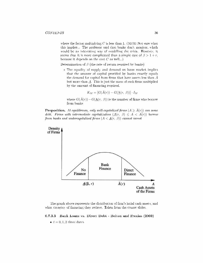
∗ The equality of supply and demand on loans market impliesthat the amount of capital provided by banks exactly equalsthe demand for capital from �rms that have assets less than Abut more than A. This is just the mass of such �rms multipliedby the amount of �nancing required.

KM = [G(A(r))−G(A(r, β))] · IM

where G(A(r))−G(A(r, β)) is the number of �rms who borrowfrom banks

Proposition. At equilibrium, only well-capitalized �rms (A ≥ A(r)) can issuedebt. Firms with intermediate capitalization (A(r, β) ≤ A < ¯A(r)) borrowfrom banks and undercapitalized �rms (A < A(r, β)) cannot invest

The graph above represents the distribution of �rm's intial cash assets, andwhat category of �nancing they recieve. Taken from the course slides.

0.7.3.3 Bank Loans vs. Direct Debt - Bolton and Frexias (2000)

• t = 0, 1, 2 three dates

CONTENTS 37

• Risk neutrality

• Firms have an investment project

� t = 0, outlay of 1

� t = 1, project return in case of success = y, with probability p, incase of failure = 0, with complementary probability

∗ then decision is made whether the liquidate. If so, the payo� isA.

� t = 2, if the �rm wasn't liquidated, project return in case of success= y, with probability p′, in case of failure = 0, with complementaryprobability

Success Failure Probability(success) Probability(failure

t = 1 y 0 p At = 2 y p0 p′ 0

• p ∼ [p, 1] with p < 1/2, and is publicly observable (think of it as somthinglike a credit rating.)

• p′ is private the �rm's private information, observable at t = 0, and cantake the two values {0,1}. For bad �rms it is 0, and for good �rms 1. Wemight expect that this will cause adversee selection.

• p, p′ are drawn independently

� At date 0, creditor's prior beliefs about the value of p′ are that p′ = 1with probability v

E(p′) = v

� the true value of p′ is revealed at time 1 to the bank and at time 2to other securityholders

• Firm's 3 �nancing choice, assuming no combinations of �nancial instru-ments

1. Bond �nancing

� repay �xed amount R at date 1, in case of success, and nothingat date 2. f there is a default at date 1, �rm is declared bankruptand is liquidated, yielding a return of A.

� Assumption (says that in expectation, the project will pay o�enough at date 1 to repay the date 0 investment of 1 unit ofcurrency):

E(projectcashflowt=1) > 1

⇐⇒ py + (1− p)A > 1

CONTENTS 38

The zero-pro�t condition for investors:

pR+ (1− p)A = 1

and the expected pro�t of good �rms �nanced with bonds (B):

ΠB = Πt=1B + Πt=2

B

ΠB = p(y −R) + py

together imply that

ΠB = p

[y −

(1− (1− p)A

p

)]+ py

⇐⇒ ΠB = 2py − 1 + (1− p)A

2. Equity �nancing

� a share a ∈ [0, 1] of the cash�ows sold to investors

� the zero pro�t condition for ouside shareholders:

a(py + vy) = 1

and the expected pro�t of good �rms �nanced with equity (E):

ΠE = Πt=1E + Πt=2

E

⇐⇒ ΠE = (1− a)(py + y),

together give

⇐⇒ ΠE =

(1− 1

py + vy

)(py + y)

⇐⇒ ΠE =

(y − 1

p+ v

)(p+ 1)

3. Bank debt

� repay R at time 1 in case of success and nothing at time 2. Ifthese is a default at time 1, there is a renegotiation and thebank is able to extract the whole surplus at time 2.

� zero-pro�t condition for banks where γ is the intermediationcost

1 + γ = Rp+ (1− p)[vy + (1− v)A]

⇐⇒ 1 + γ = Rp+ (1− p)[A+ v(y −A)]

expected pro�t of the �rm when �nanced with a bank loan is

ΠBL = p(y − R) + py

CONTENTS 39

� Together, the result will be that the preference between thesethree types of �nancing will be determined by what we termedthe credit risk p and the dilution costs v.

Part II

The Industrial OrganizationApproach

40

CONTENTS 41

0.8 Introduction

The Industrial Organization (IO) view of banking reduces a bank to a normal�rm. In this approach our perspective is that a bank is a �rm in the businessof producing deposits and loans.

0.9 Perfect Competitive Banks

0.9.1 Financial Sector

• N banks indexed by i = 1, 2, 3, ..., N

• Production of deposits (D) and loans (L).

� There is a cost function C(D,L) common to all banks. AssumeC”(�) > 0 (convexity) and twice-di�erentiability

• Bank n's balance sheet looks like

Assets Liabilities

Rn = Cn +Mn

(Reserves) Dn

Ln (Deposits)(Loans)

• where Mnis the bank's net position on the interbank market and

• Cnis the bank's cash reverves at the central bank

� Cn ≥ αDnwhere αis the coe�cient of compulsory reserves

0.9.2 Interaction with the real sector

Comprised of households, �rms, and governmentThe relationship between the di�erent agents can be represented as in the

following diagram

CONTENTS 42

0.9.3 Credit Multiplier Approach

• Monetary base M0is

M0 =

N∑i=1

Cn

= α

N∑i=1

Dn

= αD

=⇒ D =M0

α

and because D = M0 + L in aggregate,

L = M0

(1

α− 1

).

• therefore∂D

∂M0=

1

α> 0,

∂L

∂Mo=

1

α− 1 > 0.

• In a competative market, banks take all prices as given:

� rD is the interest rate on deposits

� rLis loan interest rate

CONTENTS 43

� r is the interest rate on the interbank market

• The pro�t optimization problem for each bank (we drop the subcript nto avoid clutter)

maxD,L

Π = rLL+ rM − rDD − C(D,L)

s.t. M = D − L− αDyields the FOCs

∂Π

∂L= rL − r −

∂C

∂L(D,L) = 0

∂Π

∂D= r(1− α)− rD −

∂C

∂D(D,L) = 0

These conditions say that each bank will adjust its volume of loans anddeposits so that the �intermediation margin,� rL − r and r(1 − α) − rDequal its marginal management cost, ∂C/∂(�).

• an increase in rD implies a decrease in the bank's demand for deposits,while an increase in rL means the bank would increase its supply ofloans... (while this makes intuitive sense, I need some help understandingthe math here, maybe second order conditions?)

• We solve for equilibirum by clearing the interbank market. Assume thateach bank n,

� Ln(r, rL, rD) is the loan supply function

� Dn(r, rL, rD) is the deposit demand function

• I(rL) is the aggregate investment demand of �rms

• S(rD) is the savings function of households

• Then the set of equilibrium interest rates {r, rL, rD} is determined by theclearing conditions:

I(rL) =

N∑i=1

Ln(r, rL, rD) (loans market)

S(rD) =

N∑i=1

Dn(r, rL, rD) +B (deposits market)

N∑i=1

Ln(r, rL, rD) = (1− α)

N∑i=1

Dn(r, rL, rD) (interbank market)

Where B is the net supply of treasury bills. Let's solve for equilibriumassuming the cost function is linearly seperable, for example

C(D,L) = γDD + γLL.

CONTENTS 44

Then the FOCs become

∂Π

∂L: rL − r = γL

=⇒ rL = r + γL

∂Π

∂D: r(1− α)− rD = γD

=⇒ rD = r(1− α)− γD.

• We will input these expressions into the market clearing conditions. Theclearing condition for the interbank market

N∑i=1

Ln(r, rL, rD) = (1− α)N∑i=1

Dn(r, rL, rD)

gives=⇒ I(rL) = (1− α)[S(rD)−B)]

into which we substitute the expressions for interest rates we determinedin the FOCs above:

I(r + γL) = (1− α)[S(r(1− α)− γD)−B],

which implicitly determines r.

Proposition 1. An increase in B (the net supply of treasury bills) entails adecrease in loans and deposits. However the absolute values are smaller thanin the standard model: ∣∣∣∣∂D∂B

∣∣∣∣ < 1;

∣∣∣∣ ∂L∂B∣∣∣∣ < 1− α

If the reserve coe�cient α increases, the volume of loans decreases, but thee�ect on deposits is ambiguous.

Proof. We will prove the �rst inequality only. The second is left as an exercisefor the reader. Use the expression we had which implicitly determines r:

I(r + γL) = (1− α)[S(r(1− α)− γD)−B].

but

I(r + γL) = I(rL) =

N∑i=1

Ln(r, rL, rD) = (1− α)

N∑i=1

Dn(r, rL, rD)

by the market clearing conditions, and since∑Ni=1Dn(r, rL, rD) = D, we

can write

CONTENTS 45

D = S(r(1− α)− γD)−B

=⇒ ∂D

∂B= (1− α)S′(r) �

∂r

∂B− 1

and we can compute ∂r/∂B by taking the partial derivative of

S(r(1− α)− γD) =I(r + γL)

1− α+B

=⇒ (1− α) � S′(r) �∂r

∂B=

1

1− α� I ′(r) �

∂r

∂B+ 1

⇐⇒ ∂r

∂B=

1

(1− α)S′(r)− 11−αI

′(r).

substituting this into our expression for ∂D/∂B:

∂D

∂B= (1− α)S′(r) �

1

(1− α)S′(r)− 11−αI

′(r)− 1

=(1− α)S′(r)− (1− α)S′(r)− 1

1−αI′(r)

(1− α)S′(r)− 11−αI

′(r)

=1

1−αI′(r)

(1− α)S′(r)− 11−αI

′(r)> −1

0.9.4 Monopolistic Bank (Monti-Klein Model)

A monopolistic bank doesn't take prices as given.

• Assume an inverse loan demand function rL(L)

• and an inverse deposit supply function rD(D)

• Assuming the interbank rate r is given for bank. The bank's pro�t opti-mization is

maxD,L

Π = [rL(L)− r]L+ [r(1− α)− rD(D)]D − C(D,L)

which yields the FOCs:

∂Π

∂L= r′L(L) + rL(L)− r − ∂C

∂L(D,L) = 0

∂Π

∂D= r(1− α)− rD(D)− r′D(D)D − ∂C

∂D(D,L) = 0

CONTENTS 46

• Elasticities εLandεD

εL =rLL

′(rL)

L(rL)

εD =rDD

′(rD)

D(rD)

• The solution (rD∗, rL∗)is characterized by

r∗L − r − ∂C∂L

r∗L=

1

εL(r∗L)

r(1− α)− r∗D − ∂C∂D

r∗D=

1

εD(r∗D)

• See slides 12-34 for the remainder of this lecture

0.9.4.1 Model

• In the following model, borrowers are also depositors. Each borrower hasa �xed loan demand of size L < 1. If there are insu�cient deposits tocover the aggregate demand for loans, the bank can borrow additionalfunds from the money market and lend these to borrowers. Likewise(conversely) any excess of deposits over the loan demand can be investedin the moeny market.

• Transportation cost parameters

� tDfor deposits, all of which are of size 1

� tLfor loans, which are of size L < 1.

• We can solve for equilibrium when contracts must be independent. Fora borrower to prefer i to i+1:

(1 + riL)L− tL(xi) ≥ (1 + ri+1L )L− tL

(1

n− xi

)

0.9.5 The Threat of Termination (Bolton and Scharfstein,

1990)

If an audit is impossible, how else can we give a borrower incentives to repay?What could be an incentive device in this case? Bolton and Scharfstein (1990)explores repeat borrower-lender relationships with the �threat of termination�being used to incentivize borrowers. Another example is Jappelli, Pagano, andBianco (2005) which looks at judicial enforcement through the legal system.

The model:

• Three dates: t = 0, 1, 2.

CONTENTS 47

• The production techology allows the borrower to invest 1 at date t, andat t+1 the borrower can get binomial cash �ow y

t t+1

−1 ywhere

y =

{yH with probability pH

yL with probability pL = 1− pH

and where E(y) > 1, and yL < 1. Cash�ows are i.i.d. across dates. Theyare not observable, so there is moral hazard.

• Entrepreneur has no wealth (A = 0 in our notation) and is risk-neutral.

• The bank can terminate the loan at t = 1 if the borrower cannot repay.

� with only 1 period credit rationing, the situation would be ine�cient,lender would only expect to get yL

• Let's calculate the expected present value of the bank pro�t. Note thatdate 2 is the �nal date. Since y is not observable this means at date 2 thebank always gets back yL. Let R be the amount speci�ed in the contractto be paid to the bank by the entrepreneur at date 1. Then we can write

π = −1 + (expected returnt=1) + P(not liquidated)× (−1 + yL)

⇐⇒ π = −1 + pHR+ pLyL + pH(−1 + yL)

⇐⇒ π = −1 + pLyL + pH(R− 1 + yL)

⇐⇒ π = pH(R− 1) + yL − 1.

• Write ICborrower:

pH(yH−R)+pL(0)+pH [pH(yH−yL)]+pL(0) ≥ pH(yH−yL)+pL(0)+0

⇐⇒ yH −R+ pH(yH − yL) ≥ (yH − yL)

⇐⇒ −R+ pH(yH − yL) ≥ −yL⇐⇒ R ≤ yL + pH(yH − yL)

⇐⇒ R ≤ pHyH + (1− pH)yL

⇐⇒ R ≤ E(y).

• The PClender:

π ≥ 0 ⇐⇒ pH(R− 1) + yL − 1 > 0

⇐⇒ R ≥ 1 +1− yLpH

.

CONTENTS 48

• Combining ICborrower and PClender,

1 +1− yLpH

≤ R ≤ E(y)

⇐⇒ 1− yL ≤ pH [E(y)− 1]

But we might ask: is this renegotiation-proof? The bank will lose (for certain)1− yLin the last period. and the borrower gains pH(yH − yL).

• Note: di�erence between default and renogatiation. Yes, the bank woulddefault if it could, but we assume that contracts are enforcible. BUT,the bank would try to renegotiate. If pH(yH − yL) < (1 − yL) impliespHyH + yL(1− pH) < 1 (negative npv), the bank might want to just paydirectly. But if this were true, the project would have negative NPV.

• Even if it's a social improvement, there's no way the borrower can transfermore than yL to the bank, no renegotiation possible, so the threat oftermination is credible.

• �Commitment� here referes to the commitment not to renegotiate, notthe commitment not to default. We assume the bank cannot default.Ex. In Townsend paper, we need full commitment.

0.9.6 Judicial Enforcement (Japelli, Pagano, and Bianco,

2005)

The idea of the following model is that the e�cacy of the legal system matters.How might the judiciary system impact the terms and availabilty of credit?Perhaps the cost and length of trials have an impact, maybe the degree ofprotection given to the borrower determines the borrower's opportunities torenegotiate the contracted repayment.

Model:

• An economy where the interest rate is normalized to zero and all agentsare risk neutral

• Investment project: an initial investment of 1 generates a cash �ow:

y =

{yH with probability p

yL with probability 1− p

• success/failure is observable.

• C is amount required to be pledged as collateral

• The �strictness� of the judicial system is modelled using two parameters:{∅p recovery rate on the firm′s cash flow

∅c recovery rate on the external collateral

CONTENTS 49

• Using these, we can compute the lender the expected repayment to thelender

pmin(R,∅py + ∅cC) + (1− p) min(R,∅cC)

If you ask for repayment of more than the proportion of what the borrowerhas left over when they default, they strategically default.

• When R ≤ ∅py+∅cC (it is not optimal for the borrower to strategicallydefault), the lender's expected payo� simpli�es to

pR+ (1− p) min(R,∅cC)

yeilding the break even condition (with equality, assuming a competitivelender):

1 = pR+ (1− p) min(R,∅cC).

Note that here, default was also assumed to be an option when state Loccurs.

� 3 cases

∗ High collateral:∅cC > 1 (the loan is fully collateralized)

∗ Too little collateral:R ≤ ∅py + ∅cC, So the maximum repay-ment the lender can get is: p(∅py + ∅cC) + (1 − p)∅cC < 1.Thus we cannot fund the project.

· if repayment of cash�ows is well enforced ∅p = 1, NPV >O, then �nanced.

∗ In intermediate case, R > ∅cC, because∅cC is smaller than 1

� If there is a huge amount of collateral, no problem, but too littlecollateral immplies credit rationing (projects that would create valuecannot be �nanced). So if repayment of cash�ows is well enforced∅p = 1, NPV > O, then �nanced, but in an economy where this isnot well enforced, collateral must be large to be �nanced.

Strategic Default: Case of Sovereign Debtor

• A country borrows L at rate r to make an investment

• Output produced is f(L).

• Static pro�t maximization determines optimal loan LD:

LD = arg maxπ = f(L)− (1 + r)LL

⇐⇒ f ′(LD) = 1 + r.

CONTENTS 50

• Dynamic case: (the opportunity cost of default equals the present valueof foregone pro�ts):

V (L) =

∞∑t=1

βt[f(L)− (1 + r)L]

=β

1− β[f(L)− (1 + r)L].

here, the exclusion from the borrowing market (threat of termination)is the only incentive to discourage default. The punishment is beingexcluded from capital markets forever.

• . β1−β (f(L)− (1 + r)L) ≥ (1 + r)L, implies f(L)

L ≥ 1+rβ .

� we noted f(L)L < f ′since it's a concave function. L ≤ L since it's a

concave function.

• When β is large enough, the optimal loan LD is feasible.

• But when β is small, L may be smaller than LD

• Example: if you are a govt and your utility is your prob of election, youcare about the short run... you might, say securitize future revenues orsomething like this, or postphone future expenses (beta is small...i.e. youdiscount the future a lot...�Impatience�) There is a retrospective votingleterature (for example Nordhaus in the 50s)

• Now considering a more complete in�nite horizon.

� Now the country borrows to smooth consumption, since there areexogenous shocks to production (stochastic production process)

� The objective function of the borrowing country is

U = E

( ∞∑t=0

βtu(Ct)

)

� Borrowing is short-term, and any default is followed by permanantexclusion from future borrowing. Let b ∈ B denote the amount of aloan, B is the set of all possible loans.

� In the case of default, the continnuation utility of the defautingcountry is

Ud = E

( ∞∑t=0

βtu(yt)

)

=Eu(y)

1− β.

CONTENTS 51

� Strategic default occurs i�

u(y) + βUd > u(y −R) + βVr

where R is the repayment amount and Vr is the continuation pay-o� associated with repaying the current period loan. The aboveexpression is equivalent to

y < ϕ(R)

where ϕis an increasing function.

� For a given y, the borrowing amount b(y) solves

V (y) = maxb∈B{u(y + b) + βEy′ [max(u(y′) + βUd, u(y′ −R(b)) + βVr)]}

where y′is the unknown future output.

� Equilibrium is characterized by {V (y), b(y), ϕ(R), R(b)}such thatthe expression for V (y) above is satis�ed where the maximum isobtained for b = b(y) and Vr = E[V (y)].

� y′ < ϕ(R) then we have strategic default.

� for all b ∈ B,

R(b) =(1 + r)b

P{y > ϕ[r(b)]}meaning that lenders behave competitively.

� Note that in this setup, the maturity of the loans are each only forone period...(This was the �canonical model� of sovereign borrowing)

Returning to the standard moral harard setting:

• Consider a static borrower-lender relationship. Both agents are risk-neutral. Suppose a borrower's return y is observable. The return's dis-tribution is a�ected by some action, say e�ort.

• let f(y, e) be the density function of the return y for a given level of e�orte. This action is unobservable by the lender.

• The borrower's cost of e�ort is given by ψ(e), increasing and convex.

• Loan contract specifying R(y).

• Denote the borrower's net expected utility by V (R, e)

V (R, e) =

ˆ(y −R(y))f(y, e)dy − ψ(e).

CONTENTS 52

• The optimal contract is determined

maxV (R, e∗)e∗

e∗ = arg maxV (R, e) s.t.

0 ≤ R(y) ≤ y, ∀yE[R(y)|e∗] ≥ U0

L

where U0Lis the minimum return demanded by the lender.

Proposition 2. If for all e1 > e2, the likelihood ratio f(y,e1)f(y,e2) is an increasing

function of y (monotone likelihood ratio (MLR) property), the optimal repay-ment function is always of the following type

R(y) =

{0 for y ≥ y∗y for y < y∗

This is non-increasing! So it's not a standard debt contract. After a threshold,the optimal repayment drops to 0. The reward is as much as possible in thegood state, and the punishment as harsh as possible in the bad state.

Proof. We �nd R* and e* from the maximization programadmit without proof that we can replace the maximization constraint with

the FOC∂∂eV (R, e∗) = 0then we can just

max

ˆ(y −R(y))f(y, e)dy − ψ(e)

s.t.

ˆ(y −R(y))fe(y, e)dy = ψ′(e)

ˆR(y)fe(y, e)dy = U0

L

L =

ˆ(y −R) + λ(y −R)fe(y, e) + µRf(y, e)]dy + [(µ− 1)f(y, e)− λe(y, e)]R

Rf(e, y)(µ− 1− λfef

)

R(y) = y

fe/f < someconstant

R(y) = 0

...something here was lost at the very end...

CONTENTS 53

• A little disappointing, but if we constrain the contract to be increasing(R must be increasing) we recover the standard debt contract.

Complete contract vs. Incomplete contracts

• Complete contracts are contracts that are contingent on all future statesof nature. Writing complete contracts will improve e�ciency, however, itis often too di�cult (and also too costly) to describe all possible futurecontingencies. Incomplete contract theory recognizes this fact.

• An incomplete contract will typically involve some delegation and allo-cation to one of the contracting parties of the power to choose amonga predetermined set of actions This power is made contingent on therealization of some veriable signals. The main insights from incompletecontract models are that the design of contracts should limit the tendencyof agents, to whom choice of actions is delegated, to behave ine�ciently...

• �No-slavery condition�/inalienability of human capital

� Noncommitment for the entrepreneur not to withdraw human cap-ital from the investment project implies some protable projects willnot be funded. The time pro�le of repayments will be a�ected bythe liquidation value of the project

� Whether this creates credit constraints or not actually depends onthe bargaining power of agents

• Simple version of the Hart and Moore model

• Look at two extreme cases

� If creditor has all the bargaining power: if Rt = yt at each date, itwill work, the lender can extract all the surplus, but no e�ciencyloss

� If entrepreneur has all the bargaining power

∗ at each date, the remainder of all the repayments must be lessthan the liquidation value

∗ Inalienablitly of human capital + entrepreneur having the bar-gaining power can create credit constraints. So liquid assetsare easier to borrow against. Inalienability is here the source ofcontract incompleteness. Think of traders, lawyers, etc. Maynot apply so much to sports.

Myers and Rajan (1998)

• the problem with illiquid assets: the one who operates the assets has thebargaining power. If an asset is very liquid, ex-post liquidation/renegotiationproblem is gone, but easy for the agent to trade against a riskier asset(do risk-shifting, asset substitution for example)

CONTENTS 54

• They claim it's a theory of banking... there's some optimal liquiditylevel... make balance sheet more illiquid, making illiquid loans with liquiddeposits.

• Model

� return of project is split between cash C and some continuation valued of the assets in place,

� C < d. (we'll see why we need this...?)

� assets can be liquidated for αd. , αis a measure of the liquidity ofthe assets in place.

� Assuming the manager has all the bargaining power implies debtrepayment must satisfy

R ≤ αd

(because otherwise the manger prefers to just liquidate and disap-pear)

∗ Manager can engage in asset substitution

· Manager gets αMd

· Investors get 0.· If

αd ≤ C + d−R

Manger doesn't engage in the asset substitution

∗ So a debt contract is feasible i�

∗R ≤ min(αd, C + d− αd)

∗ Here we've assumed that a liquid asset is easy to �steal� or riskshift, for asset with high liquidation value, it is also

∗ If your assets have low value in the hands of the manager, theyprobably have low value in the hands of someone else

· Counterexample: Liquid in hand of lenders, but di�cult todo asset substitution... (could be a port of complex deriva-tives?�...)

· Too illiquid: expost· Too liquid: incentive problems..· implies maybe there's an interior solution...

0.9.7 Securitization

• Policy Paper Bank of Japan

CONTENTS 55

� Securitization: Transform something that is not tradable into some-thing that is tradeable (a security). For example, a bank grants aloan, then sells the promises to future cash�ows to other investors.They might do this so to free up space in their capital requirementto be able to originate more loans and obtain the fees, for example.

�L D

Ebecomes

Cash DE

after securitization

∗ What are the frictions that make this make sense? (In anM&M world this wouldn't have a purpose) How it works: Cre-ation of a Special Purpose Vehicule (SPV). Perhaps if you re-ally understand the loan portfolio of the bank, but not theother activities, you might be willing to buy it for less of adiscount.

· What do bankers claim? Bankers say it's because of reg-ulation: securitizing relaxes this. Here we are talkingabout capital requirement: E < αL, and bankers hate is-suing equity... can't take anymore debt, so if want to lendmore, need to �recycle� old loans, which they percieve asa cheaper way of �nancing than issuing new equity.

∗ Issue: what are the incentives of a bank to monitor if theyjust originate and sell to the market right after? If we thoughtbanks could produce some info (perhaps from monitoring) thatmarkets couldn't, then it may be bad for welfare to fo this.

· In most cases, banks keep some a tranche of the pool ofloans they securitize to �ght against this. We can thingof this as serving a signalling purpose.

· Starting around 2001, many classes of loans that used tobe insecured, became securitized.

· When there is a boom then a bust, it means people's be-liefs varied a lot

· people seemed to believe that progress in �nancial engi-neering made markets closer to frictionless, complete mar-kets, and the securitization boom improved risk allocationwithin the world...oops! Now they say the opposite.

· More and more, banks didn't keep loans for longer thana few months. They became pure brokers, following theoriginate and distribute model...

· Gary Becker quote:

thanks to all this dream of owning a home becomestrue for many American families.

· Deregulation: Basel II...banks got to use internal models...maybe a bad idea? Self-regulation

CONTENTS 56

∗ What many banks did:

· create an Special Investment Vehicule (SIV), to whichthey would then sell a loan, and simultaneously o�ereda put to the SIV (a guarantee to buy it back at someprice) with a maturity of less than 6 months. Becauseof this short duration, a regulatory loophole meant theydidn't have to include these in their capital requirements.

· Essential problem: it was thought that information fric-tions had mostly disappeared, since the cost of info wentdown due to information technology innovations. Actu-ally the common view now is that securitization destroysa bank's monitoring incentives

· Now: Back to arbitrary, tough regulation: every bank hasto keep 5% of loan.

∗ But Maybe: There's nothing ine�ecient about it! There's atradeo� between gains from trade (possibly risk-sharing) andincentives. The increase in defaults in subprime mortgagesetc, in the standard model doesn't imply ine�ciency...

· Paper: high-documentation, but high-FICO (above 620)score borrowers are more likely to default than low-documentationborrowers with high-�co scores...implies banks are willingto lend to borrowers they know are bad since investors willbuy the securitized portfolio anyway if the FICO score ishigh enough. (whereas for below this threshold, low doc-umentation borrowers defaulted more, as you might ex-pect). Nonetheless, doesn't imply ine�ciency, in priciple.

· Plantin models of securitization: 1. Nothing ine�cient.2. Ine�cient.

• Plantin Parlour JF Paper

� The model is a variant on Holmstrom-Tirole '97 with �rms, banks,and bond-investors that we went through in class. Here, we haveone bank and many investors. In this case, �rms have constantreturns to scale, and outcomes are stochastic and dependant one�ort.

� The �rm chooses the size of the project (I), and how much bankand bond �nance it uses.

� There are 2 pieces of private info

∗ bank recieves a discount factor shock

∗ payo� from loan

CONTENTS 57

� 3 dates

∗ t = 1, 2, 3 (so 2 periods)

� risk neutral agents, who are protected by limited liability, and don'tdiscount:

∗ F �rm, has initial wealth A, and a technology transforming1 into R (or I into RI) with probability p and into 0 withprobability 1 − p if it bevaves. If the �rm shirks, p becomesp−∆p, but the �rm captures a private bene�t BF I

∗ B bank can monitor the �rm: The �rm's private bene�tBF I isdecreased to bF I < BF I, but bank recieves a bene�t BBI if itdoesn't monitor. If the bank shirks, it derives private bene�tBBI

· If the bank monitors, it �gures out the date 2 payo� atdate 1

∗ and investors (bond investors)

� 1st period, there will be a �rm e�ect, and bank's monitoring

∗ 1st case: only socially optimal thing to do is have the bankmonitor, and the �rm behaves (like if p = ∆p)

∗ The bank values liquidity. (this is like Diamond-Dybvig)

U = E(c0 + δ1(c1 + δ2c2))

where

δ2 =

{δ with probability q

0 with probability 1− q

� The �rm o�ers the optimal renegotiation-proof contracts to thebank and investors, but the bank can o�er new contracts at date 1.The �rm doesn't care what the bank does once monitoring has takenplace at date 1; the bank will trade credit risk with the investors inan ex post optimal way.

�

CONTENTS 58

� ifr =

pq

1− p+ pq< δ

where the lhs is the conditional probability of the loan being goodconditional on the fact that the bank is selling, then there is no tradein the secondary CRT market. As a real-world example, perhapsduring the 90s there was a shock lowering δ. Let

∗ I total investment, I = A+ L+M

∗ L is the money lent by banks

∗ M from investors

∗ RB and RLare as usual

�

� In the no CRT (credit risk transfer) and CRT (what if it's a poolingmarket?)...only thing that changes, no E(δ2) in their preferences,because the bank never keeps the loan through period 2. But nowif the bank shirks, it will still be able to sell something worthless.Thus, banks are willing to lend more. but now, more di�cult toinventivise banks, because they want to shirk and get the privatebene�t.

∗ Bank capital is costly, total cost of bank capital is product ofhow big their stake is and their total cost per dollar

CONTENTS 59

� For the right parameter values, in both cases, all constraints arebinding, so to solve the model just solve the PC of the bondholders.

I −A− L = pRI − bF I − pRBI

which says that the �arm's length �nance, M = I −A− L is equalto the expected payo� to bondholders. And the �rm maximizes I:

Imax =A

1− pR−unit surplus

+ bFfirm unit rent

+ pRBIMax−LIMax

bank unit rent

.

� We can see that the bank's unit rent,

pRBIMax − LIMax

can be decomposed into(pRBIMax − L

L

)× L

IMax

the price decrease with CRT times the quantity increase. And

pRBIMax

L=

1

δ1

if there is CRT, and

pRBIMax

L= − 1

δ1Eδ2

without it. Likewise,

� {L

IMax= BB

(pp−r

)if CRT

LIMax

= BB if no CRT

� We can illustrate the results on this interesting graph with 4 ar-eas: no strong connection between when it is liquid and when it ise�cient

CONTENTS 60

�

� Interpretation. Interpretδ as being dependent on p: we may wishto have a capital requirement that depends on the riskiness of theloans.

� Note that the conditions under which liquidity rises and the condi-tions under which liquidity is e�cient are NOT THE SAME.

∗ Ine�cient innovation may take place while desirable innova-tion may not. Liquidity is most likely to rise for high ratednames, for which it is ine�cient. Names which are rated toolow do not trade, though it would be desirable.

� If the rise of CRT during the 90s was driven by a fall in δ thensteeper pricing schedule of loans, but not bonds, the fraction ofbank �nance is more sensitive to credit rating.