microeconomic reform and technical efficiency in australian
TRANSCRIPT
Microeconomic Reform and Technical Efficiency in Australian Manufacturing
Neil Dias Karunaratne. Discussion Paper No. 345, April 2007, School of Economics, The University of Queensland. Australia.
Full text available as: PDF- Requires Adobe Acrobat Reader or other PDF viewer
Abstract
The technical efficiency dividend reaped by Australian manufacturing industries following the implementation of microeconomic reforms over the past three decades is analysed empirically in this paper. The technical efficiency scores have been estimated for manufacturing industries using a combined stochastic production-frontier inefficiency model that is free of simultaneity bias. The model parameters have been estimated using maximum likelihood techniques using a panel data set covering a cross-section of 8 industries spanning a time-series of 26 years (1969-1995). The empirical results shed light on how technical inefficiency in manufacturing has been whittled down by the microeconomic reform induced trade liberalisation and technology diffusion processes. Generalised likelihood ratio tests reject the null hypotheses that trade liberalisation and technology transfer had no significant impact on the reduction of technical inefficiency. The reduction of effective rate of assistance and technical efficiency and technology proxies such as intra-industry trade and capital deepening are negatively correlated during the study period. These findings give credence to the predictions of endogenous growth theories that openness of the economy provides a conduit for accessing new technology that promotes innovation and technical efficiency. The increase in technical efficiency of manufacturing industries is the unsung hero behind the emergence of the 'new economy' or the spectacular pick-up of productivity growth observed for Australia during the 1990s. The error-correction modelling reported at the outset confirms that this productivity pick-up is not an artefact of a cyclical upturn. It is attributable to the microeconomic reforms and the technology transfer that has followed it. The paper concludes on the need for further research , first, to shed light on the constituents of total factor productivity such as technical change and technical progress and second, to design policy to address the challenging issues of equity-efficiency trade-off lest it degenerates into a back-lash that could nullify the whole reform agenda.
EPrint Type: Departmental Technical Report
Keywords: trade liberalisation, technology diffusion, manufacturing industries, productivity, technical inefficiency, stochastic production frontier, panel data, translog function.
Subjects: 340000 Economics;
ID Code: JEL Classification C33, C52, D24, F12, L60, O30
Deposited By:
Neil Dias Karunaratne School of Economics The University of Queensland Brisbane Q. 4069. Australia.
e-mail: [email protected]
ISSN 1445-5523

MICROECONOMIC REFORM AND TECHNICAL EFFICIENCY IN AUSTRALIAN MANUFACTURING
Neil Dias Karunaratne* School of Economics The University of Queensland Brisbane Q. 4069. Australia.
e-mail: [email protected]
Microeconomic reforms. Trade liberalisation. Technology diffusion. Manufacturing Industries . Productivity. Technical inefficiency. Stochastic production frontier. Panel data. Translog function.
*Dr Neil Karunaratne, Associate Professor, School of Economics, University of Queensland.

3
3
I. INTRODUCTION
Australia inherited a protectionist yoke dubbed the 'Federation Tri-fecta' from the days of Federation (1901)
according to Henderson (1990). The Tri-fecta comprised of: first, strong tariff protection to shelter
domestic manufacturing industries from foreign competition; second, centralised wage-fixing and third, the
white Australia immigration policy. The protectionist Tri-fecta policies nurtured high cost manufacturing
industries catering for a small domestic market. It also sowed the seeds of Australia's downward slide on
the OECD per capita income league. Protectionist Australia's fall from its top perch as the "lucky country"
occurred at the same time when the export-oriented East-Asian economies were reporting miracle growth
rates and catching-up with Australia in the per capita income stakes. Partly as an anti-dote to Australia's
lack-lustre growth performance, a reversal from the Tri-fecta was ordained beginning with the across-the-
board 25% tariff-cut in 1973. The microeconomic reform policies spearheaded by trade liberalisation
encompassed a gamut of other initiatives such as financial deregulation, relaxing centralised wage-fixing,
corporatisation and privatisation of state enterprises, tax reform and the floating of the exchange rate.
These microeconomic reforms removed institutional and regulatory barriers that impeded the functioning of
free markets. In the free market environment manufacturing industries had either to shape up to the
challenges from global competition by adopting 'best practice' technology or go to the wall.
After thirty years of microeconomic reforms analysts are still hotly debating the pros and cons of reforms.
Some have argued that the reforms have deindustrialized Australia and the globalisation process has
marginalized large segments of the population. Critics claim that the much hyped productivity gains from
the reforms are miniscule as of the observed productivity growth rates of 0.33% per annum it would take at
least another century for Australia to reach the frontier predicted by growth theory (Quiggin,1998).
The proponents of microeconomic reform, e.g. the Productivity Commission, on the other hand contend
that productivity growth has dramatically increased in the 1990s when compared to the previous decade
causing the emergence of a 'new economy' (Parham, 1999). Independent empirical estimates based on
4
4
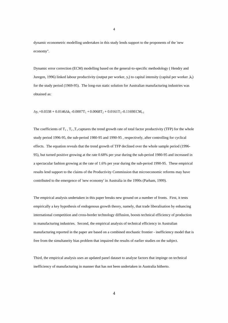
dynamic econometric modelling undertaken in this study lends support to the proponents of the 'new
economy''.
Dynamic error correction (ECM) modelling based on the general-to-specific methodology ( Hendry and
Juregen, 1996) linked labour productivity (output per worker, yt) to capital intensity (capital per worker ,kt)
for the study period (1969-95). The long-run static solution for Australian manufacturing industries was
obtained as:
Δyt =0.0338 + 0.0146Δkt -0.0007T1 + 0.0068T2 + 0.0161T3 -0.1169ECMt-1
The coefficients of T1 , T2 ,T3 captures the trend growth rate of total factor productivity (TFP) for the whole
study period 1996-95, the sub-period 1980-95 and 1990-95 , respectively, after controlling for cyclical
effects. The equation reveals that the trend growth of TFP declined over the whole sample period (1996-
95), but turned positive growing at the rate 0.68% per year during the sub-period 1980-95 and increased in
a spectacular fashion growing at the rate of 1.6% per year during the sub-period 1990-95. These empirical
results lend support to the claims of the Productivity Commission that microeconomic reforms may have
contributed to the emergence of 'new economy' in Australia in the 1990s (Parham, 1999).
The empirical analysis undertaken in this paper breaks new ground on a number of fronts. First, it tests
empirically a key hypothesis of endogenous growth theory, namely, that trade liberalisation by enhancing
international competition and cross-border technology diffusion, boosts technical efficiency of production
in manufacturing industries. Second, the empirical analysis of technical efficiency in Australian
manufacturing reported in the paper are based on a combined stochastic frontier - inefficiency model that is
free from the simultaneity bias problem that impaired the results of earlier studies on the subject.
Third, the empirical analysis uses an updated panel dataset to analyse factors that impinge on technical
inefficiency of manufacturing in manner that has not been undertaken in Australia hitherto.

5
5
Fourth, it sets the stage for undertaking the decomposition of growth of total factor productivity into its
components of technical change and technical progress in order to analyse the role of technology in the
emergent 'new economy' in the new century.
Fifth, the empirical findings highlight the counterproductive nature of the single-minded pursuit of a policy
agenda based on first-best efficiency criteria in a second-best world where equity-efficiency tradeoffs are
the order of the day.
The rest of the paper is structured as follows: Section II surveys the theoretical literature postulating links
between trade related microeconomic reforms and the increase in productivity in manufacturing industries.
This section also reviews past Australian studies on the analysis of productivity of manufacturing
industries. Section III presents an algebraic exposition of the combined stochastic frontier - inefficiency
model used for the empirical analysis of technical efficiency of manufacturing industries. The procedures
used for the maximum likelihood estimation of model parameters and the likelihood ratio tests of various
null hypotheses are also explained in this section. Section IV describes the panel database, variables and
the data sources that have been used for the empirical validation of the stochastic frontier-inefficiency
model. Section V presents the empirical results in three parts. First, the maximum likelihood estimates and
tests of model parameters are discussed. Second, test results on null hypotheses on reform and technology
transfer processes are presented. Third, the significance of the time-varying technical efficiency scores for
different manufacturing industries are reviewed. Section VI concludes by underscoring two important
policy considerations to avoid counterproductive reforms. First, the need to decompose total factor
productivity growth into its components of technical change and technical progress so to avoid flawed
policy prescriptions. Second, the need to design adjustment policies to address the equity-efficiency trade
offs that arise from the microeconomic reform agenda.

6
6
II. BACKGROUND
Theoretical perspectives
The analysis of technical efficiency in production has a pedigree that can be traced to the seminal work of
Farrell (1957) which defines technical efficiency as the production of more output with a given set of fixed
factor inputs.
The concept of efficiency is also linked to the concept of 'x-efficiency' or the increase in output through
better organisation and management (Leibenstein 1966). The literature relating to trade focussed
microeconomic reforms and efficiency gains can be discussed under three headings: Neoclassical trade
perspective, political economy of protection and endogenous or new growth theories.
The conventional or neoclassical trade theory postulates that trade liberalisation by exposing manufacturing
industries to the fresh winds of competition and by enlarging markets delivers gains in productivity and
efficiency. These gains arise from specialising according to the principle of comparative advantage for the
global market. The production for an enlarged global market generates increasing returns to scale and other
dynamic benefits resulting in sizeable cost reductions due to technical efficiencies in production. Although
some critics doubt the role of trade to act as an engine of growth , empirical studies both for Australia and
other countries vindicate the role of trade as a propeller of growth. These studies support the conventional
wisdom that free trade is first best in that it promotes efficiency and growth and maximises national and
global welfare (Karunaratne 1997).
The political economy perspective on protection of manufacturing industries contends that it leads to a
massive waste of resources to fund lobbying activities to perpetuate rent yielding protection. Lobbyist fund
the re-election maximising strategies of politicians who pay-back the lobbies by maintaining tariff and non-
tariff barriers. These measures inflict inflationary costs on the unorganised and free riding consumer and
therefore harm national welfare. The microeconomic reform strategies implemented in Australia over the

7
7
past three decades represent a sea change as there was a switch from protectionist policies nurtured under
the Federation tri-fecta to the free trade ethos favoured by the neoclassical paradigm.
Endogenous or new growth theories contend that the opening an economy to freer trade facilitates the
diffusion of new technologies through intra-industry trade by promoting horizontal differentiation of inputs
and the scaling up of the product 'quality ladder' (Keller 2000). New growth theories contend that the
exposure to international competition triggers endogenous research and development (R&D) and
innovation. Therefore technological progress is not exogenous as assumed in neoclassical (Solow) growth
theory but springs from the inner wells of industry (Romer 1990, Aghion and Howitt 1998, Grossman and
Helpman 1991). Moreover trade acts as the conduit for the transfer of new technology that increases
efficiency and growth (Barro and Sala-i-Martin 1995).
The new technology activates 'learning-by-doing' spillover effects (Lucas 1988, Young 1991) and
accelerates the process of catch-up with best practice or efficient technology as confirmed by studies on
manufacturing industries (Tybout et al. 1991).
To recap, endogenous growth theory foreshadows that microeconomic reforms liberalising trade facilitate
the transfer of new technology through intra-industry trade (IT) and promotes domestic innovation and
capital deepening bolstering productivity and technical efficiency in production.
Despite the cogent theoretical case and copious empirical evidence, there are misgivings about the
existence of a positive links between trade liberalisation and productivity growth. Empirical evidence from
developing countries is tendered to cast aspersions on the positive trade - growth nexus by Rodrik (1992).
Productivity growth in Australia, after adjusting for cyclical factors during the study period increased only
by a meagre 0.3 per cent per year, requiring 100 years to reach the upper bound postulated by growth
theory according to Quiggin (1998:97). Nonetheless, the theoretical possibility for microeconomic reforms
spearheaded by trade reforms in generating positive externalities or 'standing over the shoulders of giants'
spillover effects that could far outweigh the negative externalities or 'stepping over toes' spillover effects

8
8
(Mankiw 2000) leading to a strong positive trade growth link cannot be gainsaid. Some observers have
claimed that Australia has recently caught the wave of the 'new economy' due to microeconomic reforms.
The need to illuminate the debate by empirical analysis motivates this paper.
Australian studies
An important survey by Dawkins and Rogers (1998) of productivity studies of over thirty manufacturing
industries undertaken over the past two decades, hereafter referred to as the Survey , classifies the findings
under three broad headings: micro, meso and macro studies. The micro level case studies examined
productivity differentials between domestic and foreign firms e.g. in the manufacture of photographic paper
and water heaters and the like. The meso or industry level studies used a variety of techniques such as
shift-share analysis, econometrics, production frontiers to analyse and identify factors that retarded
productivity and efficiency in domestic manufacturing. Regression methods revealed that existence of
positive links between factor biased (labour augmenting) technical change and productivity (Whiteman
1991).
Stochastic frontier production analysis demonstrated that productivity in manufacturing was positively
linked to R&D and regional concentration (Caves, 1982). Macro level studies based on vintage capital
models elucidate that labour augmenting technical progress occurred when the growth rate of labour
productivity exceeded the positive growth rate differential between wages and rental capital (Bloch and
Madden 1994).
Studies on labour market institutions demonstrated that the corporatist Accord was less conducive to higher
labour productivity than the more decentralised wage-fixing options (Dowrick 1993). International
comparisons of manufacturing productivity disclosed that lagged behind the frontrunners like the USA by
more than 50% (Pilat et al. 1993). The Survey despite its wide coverage had some glaring omissions. For
example, it failed to review the path-breaking computer general equilibrium (CGE) policy studies
pioneered by Dixon et al. (1983), the numerous input-output studies (Karunaratne 1989) and the visionary

9
9
information economy studies initiated by Don Lamberton (see Jussawalla et al. 1988). The Survey made
three important recommendations to upgrade productivity analysis in Australian manufacturing. First, use
of modern databases beyond 1977-78. Second, analysis at a more disaggregated cross-section time series
to shed better light on the efficiency dynamics in the post-reform period. Third, the use of more robust
techniques to unravel the complex links between reform policy and productivity. The empirical analysis
undertaken in this paper attempts to addresses the important recommendations made by the Survey.
III. THE STOCHSASTIC FRONTIER-INEFFICIENCY MODEL
The stochastic production frontier model was formulated independently by Aigner et al. (1977) and
Meeusen and van den Broeck (1977) based on the theoretical insights of Farrell (1957) and others. Surveys
reveal that the production frontier has been applied to analyse technical efficiency in agriculture, health,
education, business, military, banking and many other areas (Lovell 1993,Green 1997). It should be noted
that stochastic frontier modelling of technical efficiency differs from Data Envelopment Analysis (DEA) -
the deterministic approach to productivity analysis based on linear programming .
Conceptually technical efficiency describes the shortfalls in production from the maximum capacity output
level or the output on the production frontier. Movements of the production frontier over time describes the
concept of technical progress.
Both technical efficiency and technical progress combine to explain total factor productivity growth. The
methodology of stochastic production frontier applied in this paper focuses mainly on the analysis of
technical efficiency. A noteworthy feature of the combined stochastic frontier -inefficiency model used in
the empirical analysis in this paper is that it is free of the simultaneity bias that vitiated estimates of
technical efficiency used in earlier studies. For example, the two-stage method used by Pitt and Lee (1981)
and Kalirajan (1981) was deficient as the technical efficiency estimates were afflicted by simultaneous
equation bias. The bias free methodology for the simultaneous estimation of the stochastic production
frontier and the inefficiency effects model used in the empirical analysis reported in this paper is based on

10
10
the exposition by Coelli et al. (1998). The methodology has been applied using panel data to analyse
technical efficiency in a developing country agriculture by Battese and Coelli (1995) and in a developing
country manufacturing by Lundwall and Battese (2000). In this paper, the results of the first application of
the combined stochastic frontier production frontier - inefficiency model to analyse technical efficiency of
Australian manufacturing industries using a comprehensive panel dataset is presented.
The empirical validation of the combined stochastic production frontier-inefficiency model required the
implementation of a number of steps. First, tests had to be performed to determine whether the stochastic
frontier model was really an advancement over the average response function or a deterministic model with
no technical inefficiency.
Second, the appropriate functional form for the stochastic frontier model had to be determined from
specifications such as the Cobb-Douglas (CD) function with constant returns to scale and the Translog (TL)
with variable elasticity of factor input substitution. Third, numerous null hypotheses relating to
significance of subsets of parameters had to be tested to establish whether it was trade reforms or
technology that was making a dent on the reduction of technical inefficiency.
The above null hypotheses were tested using the generalised likelihood ratio (LR) test LRcal = − 2[lnL(H0)
-lnL(H1)], which was distributed as chi-squared distribution with the degrees of freedom determined by the
number of parameter restrictions. Therefore the critical values (CVs) to test the null hypotheses were read
off the chi-squared table and has been presented as LRtab in Table 3.
The stochastic production frontier model could be defined as :
YNTx1 = X NTxK β Kx1+ ε NTx1 (1)
Y NTx1 : Value-added at constant prices of a panel of NTx1.
where NT=208, given N=8 industries (cross-section), T=26 years (time-series).
11
11
X NTxK : NTxK =208x 3. K=Factor inputs: capital (K) , labour (L) and time (T).
β Kx1 : Maximum likelihood estimates of the K parameters.
ε NTx1 = VNTx1 + UNTx1 (composite error term) relating to vector of NT=208 observations, where V NTx1
refers to stochastic errors and UNTx1 to the technical inefficiency effects with distributions as specified
below.
VNTx1 ~ iid N( 0, σ2v) NT stochastic errors ( independently distributed of UNTx1)
UNTz1 ~ iid N( μ, σ2u) NT technical inefficiency effects distributed truncated normal.
The distribution has mean μNTx1 =ZNTxQ'δQx1, where the vector ZNTxQ represents proxy variables explaining
the technical inefficiency effects UNTx1 . The associated parameters δQx1 are estimated simultaneously with
the stochastic production frontier model thus expunging simultaneity bias.
The mean inefficiency effects model for the panel , where W ΝΤx1 is the stochastic error can be defined as:
μΝΤξ1 = ZNxQδQxT +WNxT (2)
The log-likelihood function of the stochastic frontier model (1) yields asymptotically efficient maximum
likelihood estimates ( Coelli et al. 1998) :
lnL ( β, γ, σ2) = -N/2[ln (π/2) −Ν/2log (σ2) + Σi=1N ln[(1-Φ(ζi)] - + Σi=1
N ln[(yi-xiβ)2] (3)

12
12
where σ2 = σu2+ σv
2; ζi =[(lnyi -xiβ)/σ][γ/(1−γ)]1/2 and Φ(.) represent the standard normal distribution
function. The first order conditions from the likelihood function (3) from the combined frontier and
inefficiency models (1) and (2) provide the maximum likelihood estimates of the parameters:
θ = ( β, δ, σ2, γ) . The total error variance of the combined model defined by σ2 = (σ2u +σ2
v ) consists of
the sum of the variance due to inefficiency effects (σ2u ) and the stochastic error (σ2 v). The proportion of
the total error variance explained by inefficiency effects is defined by ratio γ (gamma) which lies in the
range 0 ≤ γ ≤1. If γ is near unity a high proportion of the error variance is explained by technical
inefficiency effects.
γ = σ2u /σ2 (4)
The technical efficiency (TE) is measured by the non-negative random error vector UNTx1 which is
distributed iid (independently, identically distributed) normally and truncated at zero with mathematical
expectation or population mean μ and variance σ2u.. The average TE is estimated by the mathematical
expectation of the exponential distribution given below:
TENTx1 = exp(-UNTx1) (5)
The maximum likelihood estimates of the time-varying industry specific technical inefficiencies are
estimated from the conditional expectation of inefficiency effects defined in equation (6) below, where E
refers to the expectations operator and exp to the exponential ( Coelli et al. 1998: 190)
E[ exp(-ui | e i] = [1−φ( σA + γ ei/σA ) exp( γei+σ2Α/2)]/[1− φ( γei/σA )] (6)
The maximum likelihood estimates of the β−parameters of the stochastic frontier model and δ−parameters
of the inefficiency model were estimated simultaneously to obtain estimates that were free simultaneous
equation bias.

13
13
IV. THE DATABASE AND MODEL VARIABLES
A comprehensive panel dataset covering a cross-section of 8 industries over a time-series of 26 years
(1969-1995) was used to validate the combined frontier-inefficiency model. The aggregation for the cross-
section of the 8 industries is based on a modified two-digit Australia New Zealand Standard Industrial
Classification ( ANZSIC) code (ABS, 1993) . The classification and industry codes are reported in Table 1.
Table 1 Manufacturing Industry ANZSIC Classification used in the study. Industry ANZSCC
ode Australia New Zealand Standard Industry Classification (ANZSIC)
Industry code
1 21 Food beverages and tobacco FBT 2 22 Textiles, clothing, footwear and leather TCF 3 24 Printing, publishing and recorded media PPR 4 25 Petroleum, coal, chemicals and associated products PCC 5 271,2,3 Basic metal products BMP 6 274,5,6 Structural and sheet metal products SMP 7 281,2 Transport equipment TEQ 8 23,26,284,
5,6.29 Other manufacturing OMF
Source: IC (1997)
Variables in the stochastic frontier model ( β− parameters)
The stochastic frontier model explains value added (Y) in terms of factor inputs capital (K) and labour (L)
and time (T). The latter variable T purports to capture Hicks neutral technical change. The combined
models specified in equations (1) and (3) have been empirically validated using the IC (1997) panel dataset
for a cross-section of N=8 industries over time-series T=26 for over NTx1 observations.
YNTx1: Value-added is measured in terms of unassisted prices, thereby providing a distortion free measure
(IC 1997:28). Value-added is gross output minus intermediate inputs. All values are measured using
unassisted constant 1989/90 prices. An index of the size of assistance measured the benefits due to tariff,
quotas, subsidies accruing to the assisted industries. The index was used to deflate market prices in order to
derive a measure of unassisted value-added, that was free of distortion.
14
14
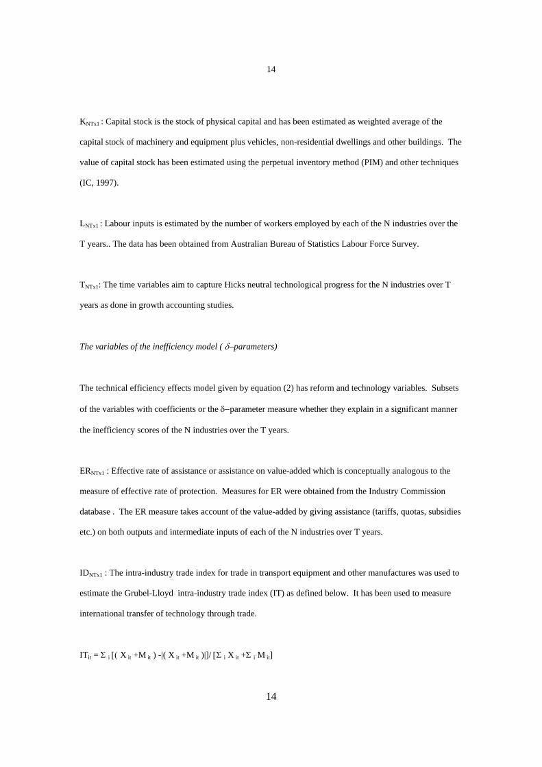
KNTx1 : Capital stock is the stock of physical capital and has been estimated as weighted average of the
capital stock of machinery and equipment plus vehicles, non-residential dwellings and other buildings. The
value of capital stock has been estimated using the perpetual inventory method (PIM) and other techniques
(IC, 1997).
LNTx1 : Labour inputs is estimated by the number of workers employed by each of the N industries over the
T years.. The data has been obtained from Australian Bureau of Statistics Labour Force Survey.
TNTx1: The time variables aim to capture Hicks neutral technological progress for the N industries over T
years as done in growth accounting studies.
The variables of the inefficiency model ( δ−parameters)
The technical efficiency effects model given by equation (2) has reform and technology variables. Subsets
of the variables with coefficients or the δ−parameter measure whether they explain in a significant manner
the inefficiency scores of the N industries over the T years.
ERNTx1 : Effective rate of assistance or assistance on value-added which is conceptually analogous to the
measure of effective rate of protection. Measures for ER were obtained from the Industry Commission
database . The ER measure takes account of the value-added by giving assistance (tariffs, quotas, subsidies
etc.) on both outputs and intermediate inputs of each of the N industries over T years.
IDNTx1 : The intra-industry trade index for trade in transport equipment and other manufactures was used to
estimate the Grubel-Lloyd intra-industry trade index (IT) as defined below. It has been used to measure
international transfer of technology through trade.
ITit = Σ i [( X it +M it ) -|( X it +M it )|]/ [Σ i X it +Σ i M it]
15
15
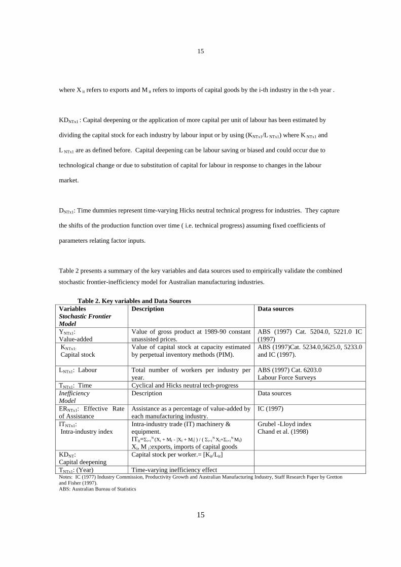
where X it refers to exports and M it refers to imports of capital goods by the i-th industry in the t-th year .
KDNTx1 : Capital deepening or the application of more capital per unit of labour has been estimated by
dividing the capital stock for each industry by labour input or by using (KNTx1/L NTx1) where K NTx1 and
L NTx1 are as defined before. Capital deepening can be labour saving or biased and could occur due to
technological change or due to substitution of capital for labour in response to changes in the labour
market.
DNTx1: Time dummies represent time-varying Hicks neutral technical progress for industries. They capture
the shifts of the production function over time ( i.e. technical progress) assuming fixed coefficients of
parameters relating factor inputs.
Table 2 presents a summary of the key variables and data sources used to empirically validate the combined
stochastic frontier-inefficiency model for Australian manufacturing industries.
Table 2. Key variables and Data Sources
Variables Stochastic Frontier Model
Description Data sources
YNTx1: Value-added
Value of gross product at 1989-90 constant unassisted prices.
ABS (1997) Cat. 5204.0, 5221.0 IC (1997)
KNTx1: Capital stock
Value of capital stock at capacity estimated by perpetual inventory methods (PIM).
ABS (1997)Cat. 5234.0,5625.0, 5233.0 and IC (1997).
LNTx1: Labour Total number of workers per industry per year.
ABS (1997) Cat. 6203.0 Labour Force Surveys
TNTx1: Time Cyclical and Hicks neutral tech-progress Inefficiency Model
Description Data sources
ERNTx1: Effective Rate of Assistance
Assistance as a percentage of value-added by each manufacturing industry.
IC (1997)
ITNTx1: Intra-industry index
Intra-industry trade (IT) machinery & equipment. ITit=Σi=1
N (Xi + MI - |XI + Mi| ) / ( Σi=1N XI+Σi=1
N MI) Xi, M i:exports, imports of capital goods
Grubel -Lloyd index Chand et al. (1998)
KDNT: Capital deepening
Capital stock per worker.= [Kit/Lit]
TNTx1: (Year) Time-varying inefficiency effect Notes: IC (1977) Industry Commission, Productivity Growth and Australian Manufacturing Industry, Staff Research Paper by Gretton and Fisher (1997). ABS: Australian Bureau of Statistics
16
16
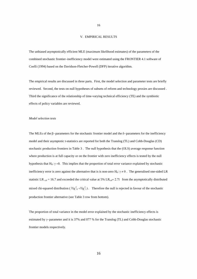
V. EMPIRICAL RESULTS
The unbiased asymptotically efficient MLE (maximum likelihood estimates) of the parameters of the
combined stochastic frontier–inefficiency model were estimated using the FRONTIER 4.1 software of
Coelli (1994) based on the Davidson-Fletcher-Powell (DFP) iterative algorithm.
The empirical results are discussed in three parts. First, the model selection and parameter tests are briefly
reviewed. Second, the tests on null hypotheses of subsets of reform and technology proxies are discussed .
Third the significance of the relationship of time-varying technical efficiency (TE) and the symbiotic
effects of policy variables are reviewed.
Model selection tests
The MLEs of the β−parameters for the stochastic frontier model and the δ−parameters for the inefficiency
model and their asymptotic t-statistics are reported for both the Translog (TL) and Cobb-Douglas (CD)
stochastic production frontiers in Table 3 . The null hypothesis that the (OLS) average response function
where production is at full capacity or on the frontier with zero inefficiency effects is tested by the null
hypothesis that H0: γ =0. This implies that the proportion of total error variance explained by stochastic
inefficiency error is zero against the alternative that is is non-zero H0: γ ≠ 0 . The generalised one-sided LR
statistic LR cal = 16.7 and exceeded the critical value at 5% LRcal= 2.71 from the asymptotically distributed
mixed chi-squared distribution ( ½χ20 +½χ2
1) . Therefore the null is rejected in favour of the stochastic
production frontier alternative (see Table 3 row from bottom).
The proportion of total variance in the model error explained by the stochastic inefficiency effects is
estimated by γ−parameter and it is 37% and 077 % for the Translog (TL) and Cobb-Douglas stochastic
frontier models respectively.
17
17
Table 3 Maximum Likelihood Estimates (MLE) Cobb-Douglas (CD) and Translog (TL) Stochastic Production Frontier Models Variable Description in natural logs
Parameter Translog (TL)
Asymptotic |t-statistic|
Cobb-Douglas (CD)
Aysmptotic |t-statistic|
Constant β0 65.62** 9.46 2.04** 3.80 Kt : Capital β1 − 9.63** 7.95 0.18** 3.74 Lt : Labour β2 6.05** 4.60 0.75** 14.59 Tt : Time β3 − 0.02 0.94 0.04** 13.31 Kt
2 : (Capital)2 β4 0.45** 8.02 − − Lt
2 : (Labour)2 β5 0.87** 11.54 − − Tt
2 : (Time)2 β6 − 0.00** 4.01 − − KtLt : (Capital x Labour) β7 − 0.89** 7.17 − − KtTt : (Capital x Time) β8 0.00 1.53 − − LtTt : ( Labour x Time) β9 0.00 0.39 − − Constant δ0 4.73** 2.31 −30.05** 4.79 ERt : (Effective rate of assistance)
δ1 5.83** 11.17 .60** 2.55
ITt : ( Intra-Industry Trade) δ2 3.50** 3.89 1.96** 2.02 KDt : (Research & Development) δ3 2.70** 3.05 4.78** 4.49 ER2 : (Nominal rate of assistance)2
δ4 - 0.19** 10.56 ⎯ 0 0.07
ITt 2 : ( Intra-Industry Trade) 2 δ5 - 0.02 0.37 − 0.08 1.29 KDt
2: (Capital Deepening) 2 δ6 0.24** 7.22 − 0.21** 4.19 ERt x ITt δ7 - 0.13** 2.48 − 0.08 1.40 ERt x KDt δ8 -.039** 9.38 − 0.12** 2.46 ITt x KDt δ9 - 0.03** 3.89 −0.10 1.29 Tt : (Time) δ10 0.02 1.30 0.03** 2.06 Σt=11
36 Dt:(Time-specific dummies)
Σt=1136δt Significant t-stat none Significant t-stat none
Variance of u (TE) σs2 0.62** 7.99 0.12** 7.85
Tech efficiency / Total variance γ 0.37** 5.52 0.77** 7.63 LL :Log-likelihood function OLS
=103.92 CD =188.96
OLS =193.92
TL =265.24
Ho: Deterministic (ARF) adequate vs Stochastic Frontier Model
H0: γ=0 H1: γ≠0
1-sided LR χ2
cal=16..79
χ2df=1,2α=
2(.05)=2.71α
Decision Rej Ho:
LR-test=χ2cal=- 2[LL(Ho) - LL
H1)]
TL vs OLS LR=χ2
cal
=142.6*4
CDvsOLS LR=χ2
cal
170.08*
TL vs CD LR=χ2
cal 152.56*
Critical value=χ2df,α
(KP):Κοdde & Palm, 1986 χ2
37, 0. 05 (KP) = 51.62
χ237 0. 05(KP)
= 51.62 χ2
42, 0. 05 = 52.56
Decision: > (Reject Ho in favour of H1)
CD> OLS Rej Ho vs
H1
TL> OLS TL> CD
Notes: OLS: Ordinary Least Squares; CD: Cobb-Douglas ; TL: Translog ; ARF: Average Response Function. ; LL: Log likelihood function. Ho: Null hypothesis; H1: Alternative hypothesis. * : Significant at 5 per cent level. ** : Significant at 1 per cent level.

18
18
The one-sided generalised LR tests report results on three separate null hypotheses tests. First, the average
response function (OLS) null was tested was tested against the Cobb-Douglas (CD) alternative. The
rejection of the null in favour of the alternative is reported as CD>OLS. Second, the average response
function (OLS) null was tested against the Translog (TL) stochastic frontier alternative. The rejection of
the null in favour of the alternative is reported as TL>OLS. Third, the Cobb-Douglas stochastic frontier
null was tested against the Translog stochastic frontier alternative. The rejection of the null in favour of the
alternative is reported as TL>CD (see last three rows of Table 3). Therefore the generalised LR tests
demonstrated that the stochastic frontier model with a Translog functional form was the best description of
the data generation process underpinning the panel dataset for Australian manufacturing.
Inefficiency affects model tests
Model (2) explains technical inefficiency effects (-TE) in terms of explanatory variables in the vector:
ZNxQ= ( ERNxQ, ITNxQ, KDNxQ), where N=8 industries and Q=3 are the effects variables.
The effects variables define effective rate of assistance (ER), intra-industry trade (IT) and capital deepening
(KD). Quadratics of the effects variables are included to capture increasing or decreasing effects over time
while the cross-product terms capture interaction terms. LR tests are used to determine whether subsets of
the effects are significant in explaining the symbiotic effects of these variables on reduction of technical
inefficiency in manufacturing industries.
The null hypotheses that effective rate of assistance (ER) has no significant effect on technical inefficiency
of manufacturing tested using the LR-test have been rejected (see row 1 Table 4).
The LR tests reveal that the null hypotheses that subsets containing effective rate of assistance (ER), intra-
industry trade (IT), (KD) have no effect on technical inefficiency on manufacturing have been rejected (see
row 2 and 3 Table 4). The null hypotheses that the effective rate of assistance (ER) and the technology
proxies relating to intra-industry trade (IT) and capital deepening (KD) have no significant effects on the
technical inefficiency on manufacturing industries is soundly rejected by the LR-tests (see last 3 rows of

19
19
Table 4). Overall the empirical results lend support to the tenets of the new growth theories that assert that
trade liberalisation by promoting the transfer of new technology and innovation improves technical
efficiency and productivity in manufacturing industries.
Table 4. Test of null hypotheses on reform and technology proxies Translog function Ηο: Null hypothesis χ2
cal χ2tab,df,α=.05 Decision
Null: No ER-effects δ1=δ5=δ7=δ8 = 0 192.86* χ232,.05=45.91 Reject
Null: No IT-effects δ2=δ5=δ7=δ9 =0 125.58* χ232,.05=45.91 Reject
Null: No KD-effects δ3=δ6=δ8=δ9 = 0 86.13* χ232,.05=45.91 Reject
Null: No IT & KD effects
δ2=δ3=δ5=δ6=δ7 =δ8=δ9=0 75.78* χ228,.05=41.31 Reject
Null: No ER & KD effects
δ1=δ3=δ4=δ6=δ7 =δ8=δ9=0 68.34* χ228..05=41.31 Reject
Null: No ER & IT effects δ1=δ2=δ4=δ5 =δ7=δ8=δ9=0 51.14* χ228,.05=41.31 Reject
Time-varying technical efficiency effects
Based on the panel dataset the parameters of the combined stochastic frontier -efficiency model (4) with a
translog functional form was estimated by maximum likelihood methods using the FRONTIER 4.1software
(Coelli, 1994). For the 8 manufacturing industries over the study period of 26 years, the average technical
efficiency (TE) score was 81% implying that manufacturing industries were operating 19% below capacity.
During the study period the lowest average technical efficiency (TE) scores of 45%, 65% and 69% were
recorded for the industries TCF , PPR, OMF which were also the recipients of the highest levels of average
effective rate of assistance (ER) of approximately 127%, 24%, 25%.respectively. Therefore, the industries
that were heavily assisted exhibited the lowest levels of technical efficiency. These findings support both
neoclassical and protectionist theories which contend that assistance or protection breeds inefficiency by
sheltering manufacturing industries from the fresh winds of international competition.
The industries with the high average technical efficiency (TE) scores greater than 97% were the resource
intensive FBT, PCC and BMP industries which were subjected to low effective rate of assistance of 11%,
17% and 14% respectively. Incidentally these were resource intensive industries in which Australia
exhibited a comparative advantage (see Table 5).

20
20
Table 5 Effective Rates of Assistance(ER) and Technical Efficiency (TE) TE FBT TCF PPR PCC BMP SMP TEQ OMF AVG SD CV AVG 0.98 0.45 0.65 0.98 0.97 0.83 0.94 0.69 0.81 0.21 26.02 SD 0.01 0.12 0.22 0.01 0.03 0.03 0.05 0.15 0.07 0.06 9.00 CV 1.43 27.27 33.33 1.44 3.29 4.05 5.43 22.09 8.15 27.84 34.58 ER FBT TCF PPR PCC BMP SMP TEQ OMF AVG SD CV AVG 10.56 126.96 24.48 17.07 13.52 31.89 48.63 25.71 37.35 38.85 104.61 SD 6.18 53.46 15.40 8.66 8.60 15.31 12.73 5.37 10.04 18.92 38.22 CV 58.54 42.11 62.91 50.69 63.63 48.02 26.19 20.89 26.89 48.69 36.54 Notes. Industry codes are as in Table 1. TE: Technical Efficiency. ER: Effective rate of Assistance. AVG: Average. SD: Standard deviation. CV: Coefficient of variation in percentage terms
The average technical TE of manufacturing industries increased from 72% to 92% when average effective
rate of assistance (ER) declined from 14% to about 9% during the study period. Therefore the efficiency
gains could be regarded as spillover effects from trade liberalisation associated with micro-economic
reforms. It is noteworthy, that the reform process incubated for nearly a decade before finally kicking-in
around the mid-1980s when the TE score raced past the industry TE average score of 81%. With the
reduction in the effective rate of assistance ( ER) and trade liberalisation both the intra-industry (IT) trade
and capital deepening (KD) increased by more than 7 -fold and 2-fold respectively. During the study
period high negative correlation coefficients were observed between effective rate of assistance and the
technical efficiency coefficients (er.te), inter intra-industry trade (er.it) and capital deepening (er.kd) e (see
bottom rows of Table 6). The negative correlation coefficients confirm that the trade reforms reducing
effective rate of assistance (ER) increased technology transfer from overseas via intra-industry trade (IT)
and facilitated capital deepening (KD) as hypothesised by the endogenous growth paradigm.
The time-varying technical efficiency scores indicated that the highly protected Textile Clothing and
Footwear (TCF) and the Printing , Publishing and Recorded media (PPM) ranked last in terms of average
technical efficiency (TE) with scores of 45% and 65% respectively.
Furthermore these two most inefficient industries, TCF and PPM had the highest coefficients of variation
(CV) of 26% and 33%. The highest average TE scores of over 97% were reported by the industries FBT,
PCC and BMP- industries in which Australia had a resource based comparative advantage.

21
21
Table 6 Technical efficiency (TE), Reform & Technology Processes Year AVG TE AVG ER AVG IT AVG KD 1969 0.72 14.03 7.37 27698.36 1985 0.82 7.91 46.93 47627.44 1995 0.92 3.91 30.21 61436.42 AVG 0.81 8.70 34.66 43437.70 cor er.te=-0.94 er.it=-0.69 er.kd=-0.94 cor te.it = 0.60 te.kd=0.94 it.kd=0.60 Notes: AVG : Average . TE: Technical Efficiency. ER: Effective Rate of Assistance. IT: Intra-industry Trade.KD: Capital deepening. Cor: correlation.
It is noteworthy that the highly protected TCF industries had a TE score of only 21% at the start of the
study period and by the end of the study period due to the scaling down of effective rate of assistance, the
TE score had risen to 64%. These results give legs to the predictions of endogenous growth theories and
the claims of the proponents of the microeconomic reform agenda that the reforms have delivered in terms
of enhance productivity and efficiency in production. But despite the noteworthy gains it needs to be noted
that the TCF industries at the end of the study period were performing 36% below the 'best practice' or the
maximum capacity level of production. The fact that TCF sector continues to heavily protected even to day
could be blamed for this outcome (see Table 7)
Table 7 Technical Efficiency of Manufacturing in Australia (1969-95) (selected years) YR/IND FBT TCF PPM PCC BMP SMP TEQ OMF AVG SD CV%
1969 1 0.21 0.47 0.99 0.99 0.75 0.91 0.43 0.72 0.3 42.8 1985 1 0.45 0.65 0.97 0.92 0.81 0.98 0.76 0.82 0.2 23.4 1995 1 0.64 0.99 0.98 0.99 0.86 0.99 0.94 0.92 0.1 13.4 AVG 1 0.45 0.65 0.98 0.97 0.83 0.94 0.69 0.81 Rank 1 8 7 2 3 5 4 6 SD 0 0.12 0.22 0.01 0.03 0.03 0.05 0.15 CV 1.5 26.8 33.3 1.5 3.25 3.99 5.3 22 RANK 7 2 1 8 6 5 4 3 Notes. Average (AVG), Standard deviation (SD) , Coefficient of Variation (CV) refer to the whole year.
The implementation of microeconomic reform policies during the study period appears to have contributed
to a monotonic improvement in the average technical efficiency in manufacturing industries. The average
TE score rose from 72% to 92% over the 26-year study period. This rise was accompanied by a

22
22
concomitant reduction in the coefficient of variation (CV) of the TE scores from an average of 43% to 13%
during the same period. The reduction in coefficient of variation (CV) in TE improves the efficient
allocation of resources in the same way that reduction in the CV of protection improves the efficient
allocation by reducing distortions in the price signal among trading nations ( Corden 1971).
The average time varying TE scores for the manufacturing sector has increased from 72% to 92% during
the study period. The TE scores accelerated during the mid-period when the micro-economic reforms
started to kick-in. The increase in TE is no doubt the unsung hero in Australia's spectacular labour
productivity pick-up observed in the 1990s. The observed northward trek of TE scores and the rejection of
the null hypotheses that reform and technology proxies had no impact on manufacturing industry technical
inefficiency lend unequivocal support to the predictions of endogenous growth theories and to the claims
that microeconomic reforms have ushered a 'new economy' in Australia.
V. CONCLUSIONS
The validation of a simultaneity bias free stochastic production frontier-technical inefficiency model for the
first time for manufacturing industries in Australia, using a comprehensive panel dataset, has provided
invaluable insights on the performance of technical efficiency. The results of time-varying technical
efficiency scores analysed over for a cross-section of 8 industries over a time span of 26 years clearly
demonstrated that the scaling down of effective rate of assistance was followed closely by improvements in
the technical efficiency in manufacturing industries. Furthermore, manufacturing industries appeared to
have absorbed new technology through intra-industry trade as demonstrated by the increase in capital
deepening - all bolstering the productivity pick up observed during the 1990s. These findings augur well
both for the microeconomic reform agenda which has copped some flak recently on the grounds that the
productivity and efficiency performance has not matched the hype of protagonists of microeconomic
reforms nor the predictions of the high profile endogenous growth theories.

23
23
Nonetheless, the empirical research highlights the need for extending the research agenda embarked in this
paper in two directions. First, the need to decompose the total factor productivity growth in manufacturing
into change in technical efficiency and technical progress. Second, the need to address the equity-
efficiency trade off that occurs in the relentless pursuit of the first-best micro economic reform policies
narrowly focussed only on technical efficiency.
The analysis in the paper by default equates technical efficiency growth with total factor productivity or the
growth of the Solow residual. However, total factor productivity growth consists of both changes in
technical efficiency and technical progress. It is possible for declining technical progress to co-exist with
increasing technical efficiency and if the former exceeds the latter we could have a productivity slowdown
on our hands due to technical regress rather than a rise in technical inefficiency. The need to dichotomise
total factor productivity into the components of technical efficiency and technical progress is imperative in
order to avoid counterproductive policy prescriptions (Nishimizu and Page, 1982).
The research initiated in this paper aims to perform this decomposition using a version of the time-varying
parameters methodology which has been applied to agriculture by Kalirajan and Obwana (1996) and others.
It is recognised that the relentless pursuit of the first-best technical efficiency microeconomic reform policy
agenda has serious limitations if it benignly neglects those marginalized by the reform process on the
premise that the trickle down paradigm will convert those who are initial losers from reform policies to
eventual winners. Properly designed microeconomic reform policies need to address at the outset issues
relating the equity-efficiency tradeoffs that arise in a second-best world lest the backlash by those injured
by reforms will put the whole reform agenda on the back burner or even send it up in smoke.
It is noteworthy that three types of policy options are advocated to cope with the equity-efficiency dilemma
that arises from the single-minded pursuit of the efficiency-only reform policy agenda. The first, the statist
option, recommends a reversal of the globalisation process by the re-imposition of protectionist barriers and
regulatory distortions. The second, the neo-liberal option (a la Washington consensus) reposes a blind faith
in the neoclassical trickle-down growth paradigm that losers will be magically transformed into winners
during the penultimate stage of the reform process (Kasper, 1999). The third, the social smoothing option ,

24
24
ruminates that pre-emptive policy design should manipulate the tax -transfer and social safety net
mechanisms to address the concerns of those injured by the reforms (Argy, 1998). The design of a reform
policy agenda in order to tackle the efficiency-equity paradox, so as to avoid destructive policy back-flips,
remains a formidable challenge that needs to be addressed by policymakers and their mentors.
25
25
REFERENCES
ABS (1993) Australian Bureau of Statistics. Australia and New Zealand Standard Industrial Classification (ANZSIC) 1993 Edition. Cat. No. 12920, AGPS, Canberra.
Aghion, P. and Hewitt, P. (1998) Endogenous Growth Theory. MIT Press. Cambridge. Mass. Aigner, D.J. and Lovell, C.A.K. and Schmidt, P. (1977) "Formulation and Estimation of Stochastic
Production Function Models." Journal of Econometrics, 6: 21-37. Argy, F. (1999) "Distributional effects of structural change: some policy implications" In Structural
Adjustment: Exploring Policy Issues. Workshop Proceedings. Canberra 21 May 1999. Productivity Commission, 39-92.
Backus, D., Kehoe, J. and Kehoe, I., (1992) "In Search of Scale Effects in Trade and Growth", Journal of Economic Theory, 58: 377-409.
Barro, R. and Sala-i-Martin, X. (1995) Economic Growth. McGraw- Hill. New York. Battese, G. E. and Coelli, T. J. (1995) " A Model of Technical Inefficiency Effects in Stochastic Frontier
Production Function for Panel Data", Empirical Economics. 20: 325-32. Bloch, H. and Madden, G. (1994) Productivity Growth in Australian Manufacturing. A Vintage Capital
Model. IRIC Discussion Paper No. 9410, Curtin University. Caves, R. (1982) "Determinants of Technical Efficiency in Australia", in Caves, R. (ed.) Industrial
Efficiency in Six Countries. MIT Press. Cambridge. Mass. Chand, S., McCalman, P. and Gretton, P. (1998) " Trade Liberalisation and Manufacturing Industry
Productivity Growth", in Microeconomic Reform and Productivity Growth. Workshop Proceedings: 239-271.
Coelli, T., Prasada Rao, D.S., Battese G.E. (1998) An Introduction to Efficiency and Productivity Analysis. Kluwer Academic Publishers. Boston/Drodrecht/London.
Coelli, T.J. (1994) A Guide to FRONTIER Version 4.1: A Computer Program for Stochastic Production and Cost Function Estimation,. Mimeo, Department of Econometrics. University of New England. Armidale.
Corden, M. (1971) The Theory of Protection. Oxford Clarendon Press. Oxford. Dawkins, P. and Rodgers, M. (1998) "A General Review of Productivity Analysis in Australia
"Microeconomic Reform and Productivity Growth. Workshop Proceedings Productivity Commission and Australian National University. AusInfo, Canberra: 195-228.
Dixon, P.B., Parmenter, B.R. Sutton, J. and Vincent, D.P. (1982) ORANI: A Multisectoral Model of The Australian Economy. North-Holland Publishing Co. Amsterdam.
Dowrick, S. (1993) Wage Bargaining Systems and Productivity Growth in OECD Countries. EPAC Background Paper No. 26, Canberra.
Dowrick, S. (1998) "Explaining the Pick-Up in Australian Productivity Performance" Microeconomic Reform and Productivity Growth. Workshop Proceedings Productivity Commission and Australian National University. AusInfo, Canberra : 121-143. Economic Perspectives 6(1): 87-105.
Farrell, M.J. (1957) "The Measurement of Productive Efficiency." Journal of Royal Statistical Society. A120, 253-81.
Greene, W. H. (1997) "Frontier Production Functions" in the Handbook of Applied Econometrics.Vol. II. Microeconomics. M.H. Pesaran and P. Schmidt (eds.). Blackwell Publishers. USA: 81-166.
Gretton, P. and Fisher, B. (1997), Productivity Growth and Australian Manufacturing Industry.Industry Commission Staff Research Paper. AGPS, Canberra.
Grossman, G. and Helpman, E. (1991) Innovation and Growth in the Global Economy. MIT Press, Cambridge, Mass.
Henderson, G. (2000) Australian Answers. Random House, Sydney. Hendry, D.F. and Doornik, J.A. (1996) Empirical Econometric Modelling Using PcGive 9.0 International
Thomas Business Press, London. IC (1997) Industry Commission (1997), Productivity Growth and Australian Manufacturing Industry.
Industry Commission Staff Research Paper. AGPS, Canberra. Jussawalla, M., Lamberton, D.M., Karunaratne, N.D. (1988) The Cost of Thinking: Information Economies
of Ten Pacific Economies. Ablex Publishing Corporation, Norwood, N.J. Kalirajan, K.P. (1981) "An Econometric Analysis of Yield Variability in Paddy Production.” Canadian
Journal of Agricultural Economics, 29: 283-294.

26
26
Kalirajan, K.P. Obwana, M.P. and Zhao, S. (1996) " A decomposition of total factor productivity growth: the case of Chinese agricultural growth before and after reform.” American Journal of Agricultural Economics, 78(2): 331-38.
Karunaratne, N.D. (1989) Australian Development Issues - An Input-Output Analysis.Avebury, Gower Publishing, Aldershot, England.
Karunaratne, N.D. (1997) "High-tech innovation, trade liberalisation and growth dynamics." Karunaratne, N.D. (1999) "Globalisation and labour immiserisation in Australia" Journal of Economic
Studies, 3(2): 82-105. Kasper, W. (1999) " Structural change , growth and 'social justice' - an essay." In Structural Adjustment.
Exploring Policy Issues. Workshop Proceedings, Canberra 21 May 1999. Productivity Commission: 125-162.
Keller, W. (2000) "Do Trade Patterns and Technology Flows Affect Productivity Growth?"The World Bank Economic Review, 14(1): 17-47
Kodde, D. A. and Palm, F.C. (1986) "Wald Criteria for Jointly Testing Equality and Inequality Restrictions", Econometrica, 54(5): 1243-48.
Leibenstein, H. (1966) "Allocative Efficiency and X-inefficiency", The American Economic Review, 56(3): 392-415.
Lovell, K. (1993) "Production Frontiers and Productive Efficiency." In The Measurement of Productive E Efficiency, Fried, H., Lovell, K., and Schmidt, S. eds. Oxford University Press, New York.
Lucas, R.E. (1988) "On the Mechanics of Economic Development", Journal of Monetary Economics, 22: 3-42.
Lundwall, K. and Battese, G.E. (2000) "Firm Size, Age and Efficiency: Evidence from Kenyan Manufacturing Firms", The Journal of Development Studies, 36(3): 146-163.
Mankiw, N.G. (2000) Macroeconomics. Worth Publishers, New York. Meeusen, W., and van der Broeck, J. (1977) "Efficiency from Cobb-Douglas Production Functions with
Composite Error”, International Economic Review, 18: 435-44. Nishimizu, M. and Page, J. (1992) "Total factor productivity growth, technological progress and technical
efficiency change: dimensions of productivity change in Yuogoslavia, 1965-78”.Economic Journal 92: 920-35. Open Economies Review, 8(2): 151-70.
Parham, D. (1999) The New Economy? A New Look at Australia's Productivity Performance.Productivity Commission Staff Information Paper. Australia. Canberra.
Pilat, D., Rao, P., and Shephard, W. (1993). Australia and United States Manufacturing. A Comparison of Real Output, Productivity Levels and Purchasing Power. 1970-89. Centre for the Study of Asia-Australia Relations, Griffith University.
Pitt, M.M. and Lee, L_F. (1981) "Measurement and Sources of Technical Inefficiency in the Indonesian Weaving Industry", Journal of Development Economics, 9, 43-64. Quarterly Journal of Economics, 106(2): 369-405.
Quiggin, J. (1998). "A growth theory perspective on the effects of microeconomic reform". Microeconomic Reform and Productivity Growth. Workshop Proceedings. Productivity Commission and Australian National University.
Rodrik, D. (1992) "The limits of trade policy reform in developing countries", Journal of Romer, P. (1990) " Endogenous Technical Change ", Journal of Political Economy, 98(5):S71-S102. Tybout, J. de Melo, J. and Corbo, V. (1991) "The Effects of Trade Reforms on Scale and Technical
Efficiency : New Evidence from Chile." Journal of International Economics 31(3-4):231-50. Whiteman, J. (1991) " The Impact of Productivity Growth and Costs of Production in Australian
Manufacturing Industries", The Economic Record 67(196) : 14-25. Young, A. (1991) " Learning by Doing and Dynamic Effects of International Trade",