Microarray experimental design and analysis

Sandrine Dudoit and Robert Gentleman

Bioconductor short courseSummer 2002

© Copyright 2002, all rights reserved

Testing

Biological verification and interpretation

Microarray experiment

Estimation

Experimental design

Image analysis

Normalization

Clustering Discrimination

Biological question

Statistics andMicroarrays

Outline• Experimental design for cDNA microarray

experiments.

• Combining data across slides for cDNAmicroarray experiments.

• Multiple testing.

• A 2x2 factorial microarray experiment.

Combining data across slides

Genes

Arrays

M = log2( Red intensity / Green intensity)expression measure, e.g, RMA

0.46 0.30 0.80 1.51 0.90 ...-0.10 0.49 0.24 0.06 0.46 ...0.15 0.74 0.04 0.10 0.20 ...

-0.45 -1.03 -0.79 -0.56 -0.32 ...-0.06 1.06 1.35 1.09 -1.09 ...

… … … … …

Data on G genes for n hybridizations

Array1 Array2 Array3 Array4 Array5 …

Gene2Gene1

Gene3

Gene5Gene4

G x n genes-by-arrays data matrix

…

Combining data across slides

D

F

BA

C

E

… but columns have structureHow can we design experiments and combine data across slides to provide accurate estimates of the effects of interest?

Experimental designRegression analysis

Experimental design

O A

B AB

Experimental design

Proper experimental design is needed to ensure that questions of interest canbe answered and that this can be done accurately, given experimental constraints, such as cost of reagents and availability of mRNA.

Experimental design• Design of the array itself

– which cDNA probe sequences to print;– whether to use replicated probes;– which control sequences;– how many and where these should be printed.

• Allocation of target samples to the slides – pairing of mRNA samples for hybridization;– dye assignments;– type and number of replicates.

Graphical representationMulti-digraph• Vertices: mRNA samples;• Edges: hybridization;• Direction: dye assignment.

Cy3 sample

Cy5 sample

D

F

BA

C

E

A design for 6 types of mRNA samples

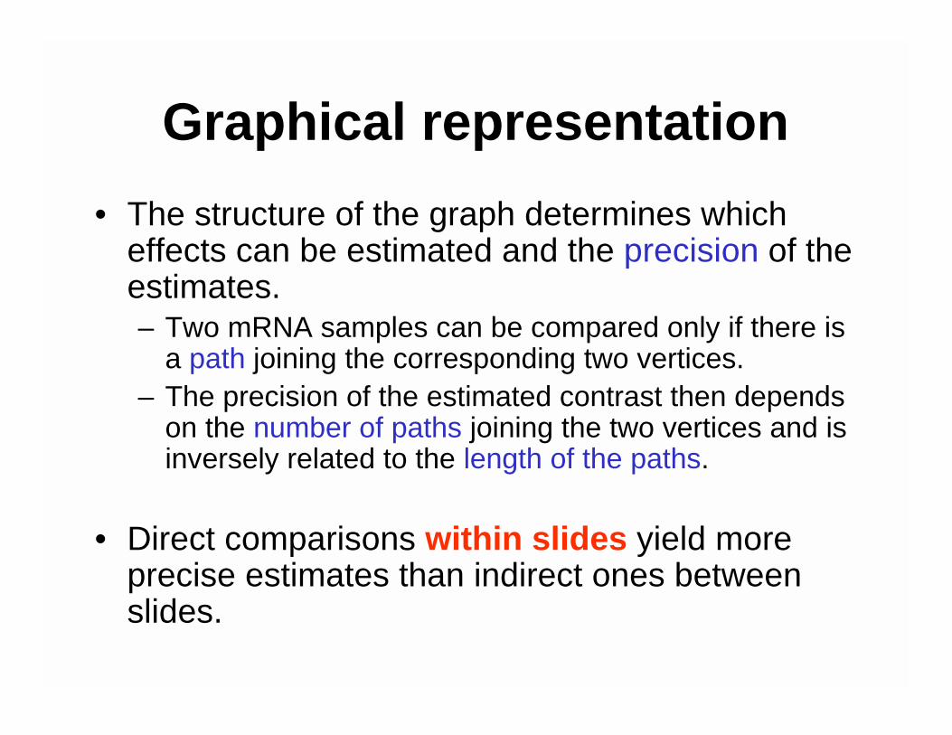
Graphical representation• The structure of the graph determines which

effects can be estimated and the precision of the estimates. – Two mRNA samples can be compared only if there is

a path joining the corresponding two vertices. – The precision of the estimated contrast then depends

on the number of paths joining the two vertices and is inversely related to the length of the paths.

• Direct comparisons within slides yield more precise estimates than indirect ones between slides.

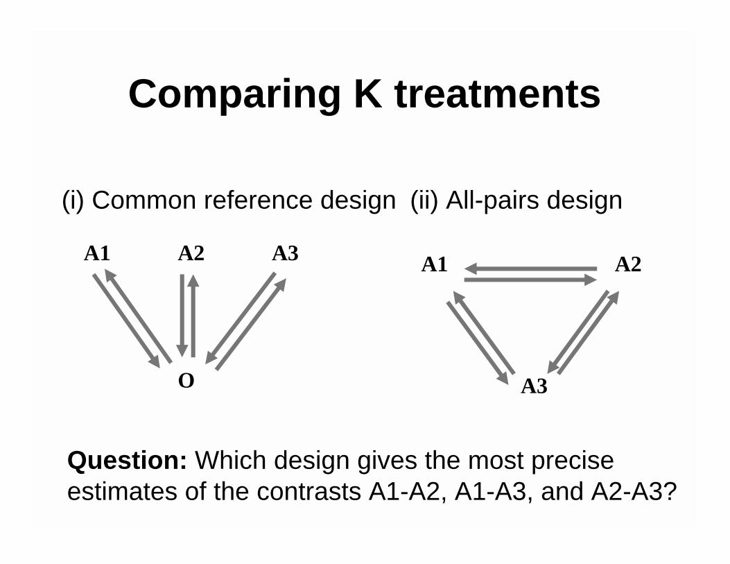
Comparing K treatments

(i) Common reference design (ii) All-pairs design

Question: Which design gives the most precise estimates of the contrasts A1-A2, A1-A3, and A2-A3?

O

A1 A2 A3 A1 A2

A3

Comparing K treatments• Answer: The all-pairs design is better, because

comparisons are done within slides.For the same precision, the common reference design requires three times as many hybridizations or slides as the all-pairs design.

• In general, for K treatmentsRelative efficiency

= 2K/(K-1) = 4, 3, 8/3, … � 2.For the same precision, the common reference design requires 2K/(K-1) times as many hybridizations as the all-pairs design.

2 x 2 factorial experimenttwo factors, two levels each

18/31

4/3(4)

14/322Contrast A-B311

(1)112Main effect A112Main effect B24/33Interaction AB

(5)(3) (2)

(1) Common ref.

Scaled variances of estimated effects

(2) Common ref. (4) Connected (5) All-pairs(3) Connected

Pooled reference

T2 T4 T5 T6 T7T3T1

Ref Compare to T1

t vs. t+3t vs. t+2t vs. t+1

Time course

Possible designs1) All samples vs. common pooled reference2) All samples vs. time 1 3) Direct hybridizations between timepoints

From Yee Hwa Yang (2002)

N=4

N=3

Design choices in time course experiments

1.67322111B) Direct hybridization

1.5121221A) T1 as common reference

t vs. t+2t vs. t+1

.75

1

1.67

2

T2T4

.75

.75

1

2

T1T4

1

.75

1.67

2

T3T4

.75

.75

.67

2

T2T3

1

.75

.67

2

T1T2

.83.75F) Direct hybridization choice 2

.831E) Direct hybridization choice 1

1.06.67D) T1 as common ref + more

22C) Common reference

AveT1T3

T2 T3 T4T1

T2 T3 T4T1Ref

T2 T3 T4T1

T2 T3 T4T1

T2 T3 T4T1

T2 T3 T4T1

Experimental design• In addition to experimental constraints, design

decisions should be guided by the knowledge of which effects are of greater interest to the investigator.E.g. which main effects, which interactions.

• The experimenter should thus decide on the comparisons for which he wants the most precision and these should be made within slides to the extent possible.

Experimental design

• N.B. Efficiency can be measured in terms of different quantities– number of slides or hybridizations;– units of biological material, e.g. amount of

mRNA for one channel.

Issues in experimental design• Replication.• Type of replication:

– within or between slides replicates; – biological or technical replicates

i.e., different vs. same extraction: generalizability vs. reproducibility.

• Sample size and power calculations.• Dye assignments.• Combining data across slides and sets of

experiments: regression analysis … next.

2 x 2 factorial experiment

O A

B AB

Study the joint effect of two treatments (e.g. drugs), A and B, say, on the gene expression response of tumor cells.

There are four possible treatment combinations

AB: both treatments are administered;A : only treatment A is administered;B : only treatment B is administered;O : cells are untreated.

two factors, two levels each

n=12

2 x 2 factorial experiment

For each gene, consider a linear model for the joint effect of treatments A and B on the expression response.

µµβµµαµµ

γβαµµ

= + = + =

+++=

O

B

A

AB

µ: baseline effect;α: treatment A main effect; β: treatment B main effect;γ: interaction between treatments A and B.

2 x 2 factorial experimentLog-ratio M for hybridization

estimates

γβµµ + =− AAB

O A

B AB

A AB

Log-ratio M for hybridization

estimates

αβµµ − =− AB

A B

+ 10 others.

Regression analysis• For parameters θ = (α, β, γ), define a

design matrix X so that E(M)=Xθ.• For each gene, compute least squares estimates

of θ.

−−

−−

−−

−

−−−

−

=

γβα

011011101101110110001001111111010010

62

61

52

51

42

41

32

31

22

21

12

11

MMMMMMMMMMMM

E

( ) MXXX ''ˆ 1−=θ

Regression analysis• Combine data across slides for complex designs

- can “link” different sets of hybridizations.• Obtain unbiased and efficient estimates of the

effects of interest (BLUE).• Obtain measures of precision for estimated effects.• Perform hypothesis testing.• Extensions of linear models

– generalized linear models; – robust weighted regression, etc.

• Use estimated effects in clustering and classification

genes x arrays matrix

genes x estimated effects matrix

Regression analysis

Multiple testing

p-value = 0.0001 ☺☺☺☺or

p-value = 5000 x 0.0001 ����

Differential gene expression• Identify genes whose expression levels are

associated with a response or covariate of interest– clinical outcome such as survival, response to

treatment, tumor class;– covariate such as treatment, dose, time.

• Estimation: estimate effects of interest (e.g. difference in means, slope, interaction) and variability of these estimates.

• Testing: assess the statistical significance of the observed associations.

Hypothesis testing• Test for each gene the null hypothesis of no

differential expression, e.g. using t- or F-statistic.Two types of errors can be committed

• Type I error or false positive– say that a gene is differentially expressed when it is

not, i.e.– reject a true null hypothesis.

• Type II error or false negative– fail to identify a truly differentially expressed gene, i.e.– fail to reject a false null hypothesis.

Multiple hypothesis testing• Large multiplicity problem: thousands of

hypotheses are tested simultaneously!– Increased chance of false positives. – E.g. chance of at least one p-value < α for G

independent tests is and converges to one as G increases. For G=1,000 and α = 0.01, this chance is 0.9999568!

– Individual p-values of 0.01 no longer correspond to significant findings.

• Need to adjust for multiple testing when assessing the statistical significance of the observed associations.

G)−− α1(1

Multiple hypothesis testing • Define an appropriate Type I error or false

positive rate.• Develop multiple testing procedures that

– provide strong control of this error rate,– are powerful (few false negatives),– take into account the joint distribution of the test

statistics.• Report adjusted p-values for each gene which

reflect the overall Type I error rate for the experiment.

• Resampling methods are useful tools to deal with the unknown joint distribution of the test statistics.

Multiple hypothesis testing

GRG-R

G1ST

Type II errorFalse null hypotheses

G0V

Type I errorUTrue null hypotheses

Rejected hypotheses

Non-rejected hypotheses

From Benjamini & Hochberg (1995)

Type I error rates• Per-family error rate (PFER). Expected number

of false positives, i.e.,PFER = E(V).

• Per-comparison error rate (PCER). Expected value of (# false positives / # of hypotheses), i.e.,

PCER = E(V)/G.• Family-wise error rate (FWER). Probability of at

least one false positive, i.e., FWER = p(V > 0).

Type I error rates

• False discovery rate (FDR). The FDR of Benjamini & Hochberg (1995) is the expected proportion of false positives among the rejected hypotheses, i.e.,

FDR = E(Q),where by definition

Q = V/R, if R > 0, 0, if R = 0.

Strong control• N.B. Expectations and probabilities above are

conditional on which hypotheses are true.• Strong control. Control of the Type I error rate

under any combination of true and false hypotheses.

• Weak control. Control of the Type I error rate under only the complete null hypothesis, i.e., when all null hypotheses are true.

• Strong control is essential in microarrayexperiments.

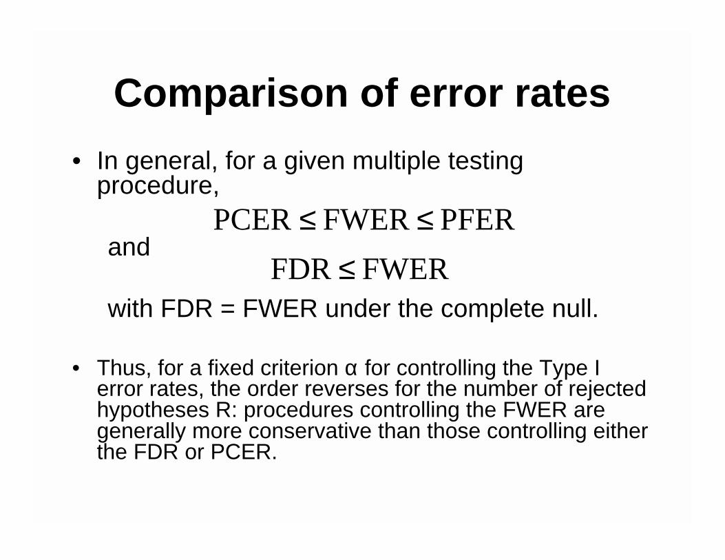
Comparison of error rates• In general, for a given multiple testing

procedure,

and

with FDR = FWER under the complete null.

• Thus, for a fixed criterion α for controlling the Type I error rates, the order reverses for the number of rejected hypotheses R: procedures controlling the FWER are generally more conservative than those controlling either the FDR or PCER.

PFER FWER PCER ≤≤ FWER FDR ≤

Adjusted p-values• Given any test procedure, the adjusted p-value

for a single gene g can be defined as the level of the entire test procedure at which gene g would just be declared differentially expressed.

• Adjusted p-values reflect for each gene the overall experiment Type I error rate when genes with a smaller p-value are declared differentially expressed.

• Can be estimated by resampling,e.g. permutation or bootstrap.

Multiple testing procedures• Strong control of FWER

– Bonferroni: single-step;– Holm (1979): step-down;– Hochberg (1986)*: step-up;– Westfall & Young (1993): step-down maxT and minP,

exploit joint distribution of test statistics.

• Strong control of FDR– Benjamini & Hochberg (1995)*: step-up;– Benjamini & Yekutieli (2001): step-up.

*some distributional assumptions required.

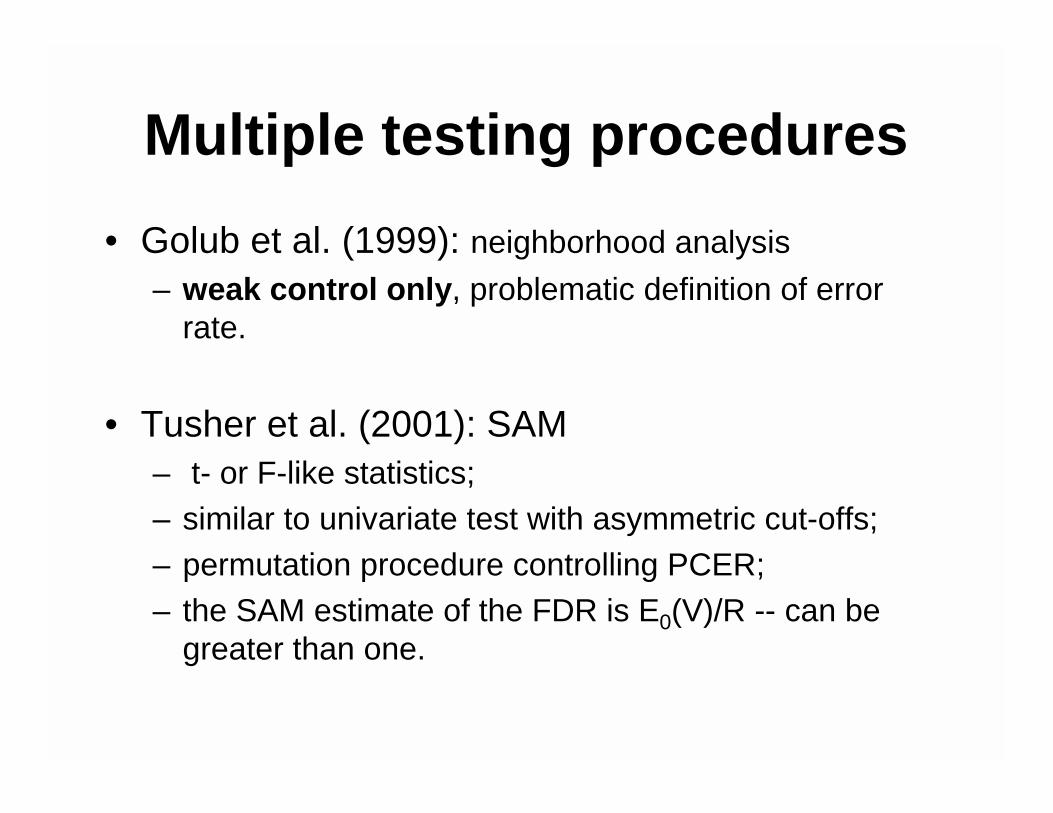
Multiple testing procedures• Golub et al. (1999): neighborhood analysis

– weak control only, problematic definition of error rate.

• Tusher et al. (2001): SAM– t- or F-like statistics;– similar to univariate test with asymmetric cut-offs;– permutation procedure controlling PCER;– the SAM estimate of the FDR is E0(V)/R -- can be

greater than one.

Multiple testing proceduresSorted adjusted p-values for different multiple testing proceduresGolub et al. (1999) ALL AML data

- FWER controlsolid lines

- FDR controldashed lines

- PCER controldotted lines

A FAQ • Q: What about pre-screening to reduce the

number of tests with the aim of increasing power?

• A: Type I error is controlled in situations where– we only focus on a subset of genes that are of interest

– selected before looking at the data;– the statistic used for screening is independent of the

test statistic under the null.• Other situations still need to be better

understood.

Discussion• Microarray experiments have revived interest in

multiple testing– lots of papers;– old methods with new names;– new methods with inadequate or unknown control

properties;– a lot of confusion!

• New proposals should be formulated precisely, within the standard statistical framework, to allow a clear assessment of the properties of different procedures.

R multiple testing software• Bioconductor R multtest package.• Multiple testing procedures for controlling

– FWER: Bonferroni, Holm (1979), Hochberg (1986), Westfall & Young (1993) maxT and minP.

– FDR: Benjamini & Hochberg (1995), Benjamini & Yekutieli(2001).

• Tests based on t- or F-statistics for one- and two-factor designs.

• Permutation procedures for estimating adjusted p-values.

• Fast permutation algorithm for minP adjusted p-values.

• Documentation: tutorial on multiple testing.

More detailed slides and references in

Multiple testing in DNA microarrayexperiments

available at www.bioconductor.org

A 2x2 factorial microarrayexperiment

Robert Gentleman, Denise ScholtensArden Miller, Sandrine Dudoit

© Copyright 2002

Complexity of genomic data• The functioning of cells is a complex and highly

structured process.• In the next slide we show a stylized biochemical

pathway (adapted from Wagner, 2001).• There are transcription factors, protein kinase

and protein phosphatase reactions.• Tools are being developed that allow us to

explore this functioning in a multitude of different ways.

Gene 1 Gene 5Gene 4Gene 3Gene 2

Pactive

P

active

DNA

protein

inactive inactivetranscription factor

protein kinase

protein phosphatase transcription

factor

An example of the interactions between some genes (adapted from Wagner 2001)

Overview• Wagner (2001) suggests that the holy grail

of functional genomics is the reconstruction of genetic networks.

• In this tutorial we examine some methods for doing this in factorial genome wide RNA expression experiments.

• Such experiments are easy to carry out and are becoming widespread. Tools for analyzing them are badly needed.

Gene effects

• A factor can either inhibit or enhance the production of mRNA for any gene.

• The inhibition or enhancement of mRNA production for any given gene can affect transcription for other genes either through inhibition or enhancement.

Targets• We define a target of a factor to be a gene

whose expression of mRNA is altered by the presence of the factor.

• A primary target is a target that is directly affected by the factor.

• A secondary target is a target whose transcription is altered only via the effects of some other genes, i.e., can be traced back to one or more primary targets.

Factorial experiments• We assume that there are two factors of interest,

F1 and F2.• A 2x2 microarray experiment can be used to

measure the expression response (mRNA level) of each gene under the four conditions– nothing– F1 alone– F2 alone– F1 and F2.

Factorial experiments

• Experimental units depend on the population of interest (i.e., for which the inference is desired). They may be cells from the same cell line, patients, or different inbred model organisms.

• Questions of interest often involve identifying which genes are directly affected by the two factors F1 and F2.

Factorial experiments• We do not just observe changes in the genes

that have been directly affected by the factors (primary targets).

• We also observe changes in any other genes whose expression levels are affected by changes in the primary targets (secondary targets).

• The addition of a judiciously chosen second factor (say one such as cyclohexamide, CX, that inhibits translation) will often allow us to isolate the primary targets from the secondary targets.

CX experiment• There are two factors

– Estrogen, E: known to affect transcription of various genes (some known, some unknown).

– Cyclohexamide, CX: known to stop all translation (with very few exceptions).

• The design is a classical 2x2 factorial design, with two replicates.

• We are interested in the main effects and interactions for E and CX.

CX experiment• We identify as targets all genes whose

expression of mRNA is affected by the application of E.

• A target can be either primary or secondary– primary if E directly affects expression of

mRNA.– secondary if mRNA production is affected by

some other gene and can be traced back to a primary target.

Scenario 1• Assume that there are two related genes,

B and D, where – B is a primary target of E,– D is a secondary target only via B.

• Neither is expressed initially.• E causes B to be expressed and this in

turn causes D to be expressed.• The addition of CX by itself may not affect

expression of either B or D.

B D

No factors applied

Gene B is not active Gene D is not active

B DE

BMRNAB

Transcription Translation

B is a Primary Target of E

D is a Secondary Target of E

MRNAD

Production of mRNABis enhanced by E

Production of mRNADis enhanced by B

B

E only

Scenario 1• In the presence of both CX and E we see

increased expression of mRNAB but not of mRNAD.

• CX stops translation of B and hence transcription of D.

• This will be one of the principles we can use to differentiate between primary targets of E (such as B) and secondary targets of E (such as D).

B DE

MRNAB

Transcription

E and CX both present

B is a Primary Target

Production of mRNABis enhanced by E

Production of mRNADis decreased (prevented)

CX

No Translation

No mRNAD

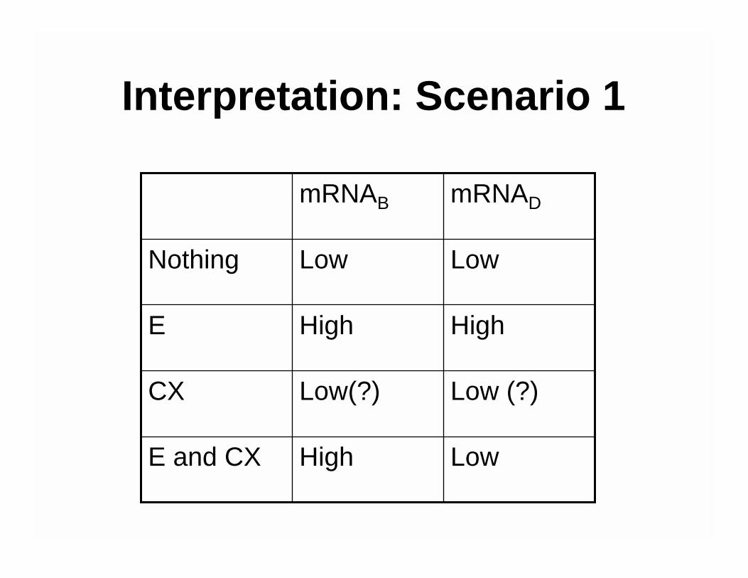
Interpretation: Scenario 1

mRNADmRNAB

LowHighE and CX

Low (?)Low(?)CX

HighHighE

LowLowNothing

Scenario 1• Note that while we show a direct

relationship between the expression of B and of D we cannot detect such a relationship from these data (the purpose of this scenario is purely pedagogical).

• Other scenarios include – Suppression of D by B, enhancement of B by

E.– Enhancement of D by B, and suppression of B

by E.

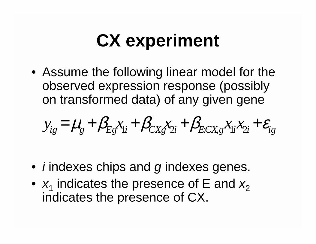
CX experiment• Assume the following linear model for the

observed expression response (possibly on transformed data) of any given gene

• i indexes chips and g indexes genes.• x1 indicates the presence of E and x2

indicates the presence of CX.

igiigCXEiCXgiEggig xxxxy εβββµ ++++= 21,:21

Inference

• The 2x2 CX microarray experiment measures the expression response of each gene under each of the four factor combinations.

• But there is a difference, B is a primary target of E, while D is a secondary target of E.

Inference• If gene X is any target for E, the level of mRNAX

might not change when E is added.• mRNAX might already be being made as fast as

possible, so addition of E has no effect.• Production of mRNAX might already be

suppressed by some other compound.• A true baseline would help in resolving these

situations.

Inference

• The introduction of CX provides a form of baseline.

• Since (among other things) CX halts translation we should be able to use the presence or absence of CX to find out about primary versus secondary targets.

Inference

• For any gene we can interpret the coefficients in the linear model as follows.

• The parameter βE can be interpreted as the main effect of E.

• Genes for which βE is different from zero are potential targets.

• As noted previously, not all targets will have βE different from zero.

Inference

• The parameter βCX can be interpreted as the main effect of CX.

• If βCX is different from zero, this suggests that production of mRNA is translationallyregulated.

• The interpretation of the interaction βE:CX is more difficult.

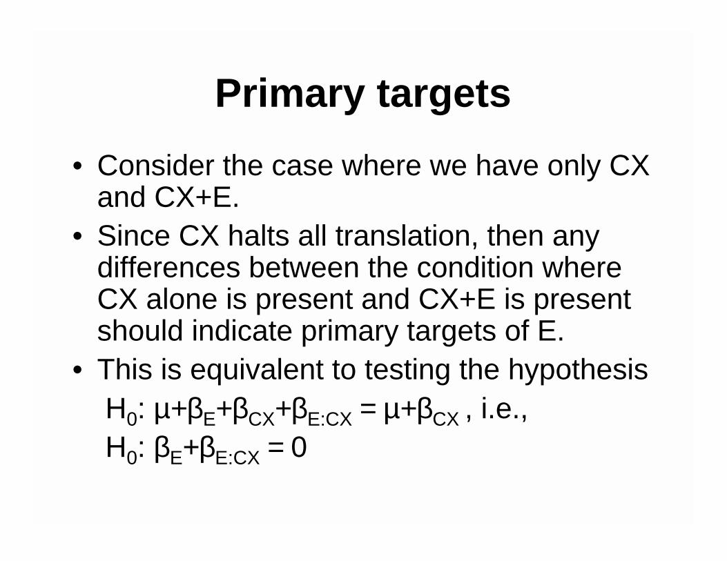
Primary targets• Consider the case where we have only CX

and CX+E.• Since CX halts all translation, then any

differences between the condition where CX alone is present and CX+E is present should indicate primary targets of E.

• This is equivalent to testing the hypothesisH0: µ+βE+βCX+βE:CX = µ+βCX , i.e., H0: βE+βE:CX = 0

Primary targets• Genes for which the hypothesis

H0: µ+βE+βCX+βE:CX = µ+βCX

is rejected are candidates for primary targets.• Those with βΕ different from zero, but for which

we do not reject H0,are secondary targets.• It seems likely that some inference may be

drawn from the relationship between βE and βE:CX, their signs and their significance levels.

Scenario 1

- βE= 0βE:CX

= 0= 0βCx

> 0> 0βE

SecondaryPrimary

Limitations• While we may identify genes that are potentially

primary targets and those that are potentially secondary targets we cannot identify gene—gene interactions, or feedback loops.

• We can observe the effects but not attribute them.

• The use of relevant metadata, biological and publication, seems pertinent and could help resolve some of the interactions.

Factorial experiments• These experiments can be contrasted with those

proposed by Wagner (2001).• He proposes perturbing each gene in the

genome of interest and observing the gene specific effects.

• We consider very few experiments and observe genome wide changes and hence less specific information.

• The two methods can be complementary since the results of the genome wide study could be used to design several single gene experiments.

Methylation experiments • Methylation inhibits transcription of specific

genes.• If a factor that demethylates the genome were

available, then one could, in principle, determine which genes were methylated (or affected by methylated genes).

• However, we could not determine which genes were primary and which were secondary targets.

Phosphorylation experiments

• Many cellular reactions are carried out using energy that is provided by the ADP-ATP phosphorylation mechanism.

• If a simple mechanism was available for halting this process then that could be used as a factor in these experiments and genes whose transcription is affected by phosphorylation could be identified.