micro- and nanoscale characterization of polymeric …evaluate fracture mechanical properties of a...
TRANSCRIPT
Micro- and Nanoscale Characterization of
Polymeric Materials by Means of
Digital Image Correlation Techniques
Von der Fakultat Mathematik, Naturwissenschaften und Informatik
der Brandenburgischen Technischen Universitat Cottbus
zur Erlangung des akademischen Grades
Doktor der Ingenieurwissenschaften
(Dr.-Ing.)
genehmigte Dissertation
vorgelegt von
Dipl.-Ing.
Jurgen Keller
geboren am 10.06.1972 in Bad Sobernheim
Gutachter: Prof. Dr. Monika Bauer
Gutachter: Prof. Dr. Bernd Michel
Gutachter: Prof. Dr. Norbert Meyendorf
Tag der mundlichen Prufung: 09.05.2005

Danksagung
Die vorliegende Dissertation entstand wahrend meiner Tatigkeit als wissenschaftlicher Mit-arbeiter am Lehrstuhl fur Polymerwerkstoffe der Brandenburgischen Technischen Univer-sitat Cottbus in Zusammenarbeit mit der Abteilung Mechanical Reliability and MicroMaterials des Fraunhofer Instituts fur Zuverlassigkeit und Mikrointegration (IZM), Berlin.
Ich bedanke mich herzlich bei allen, die zum Gelingen dieser Arbeit beigetragen haben.
Frau Prof. Dr. Monika Bauer danke ich fur die Moglichkeit, die Arbeit in ihrem Arbeitskreisdurchzufuhren, und fur den mir gewahrten Freiraum bei der Durchfuhrung der Arbeit.
Bei Herrn Prof. Dr. Bernd Michel bedanke ich mich fur die fordernde Unterstutzung unddas stete Interesse am Fortschritt meiner Arbeit.
Herrn Prof. Dr. Norbert Meyendorf danke ich fur die Ubernahme des Gutachtens und dieZusammenarbeit auf dem Gebiet der Nanodeformationsanalyse.
Herrn Christoph Uhlig und Herrn Dr. Olaf Kahle gilt mein Dank fur die wertvolle Ein-fuhrung in das Verfahren der optischen Rissspitzenerfassung (OCT), was gewissermaßendie Initialzundung der Promotion ausmachte.
Herrn Dr. Dietmar Vogel danke ich fur die Vorleistungen, die zum Gelingen des Verfahrensder SPM-basierten Deformationsmessung wesentlich beigetragen haben. Insbesondere diewertvollen Anregungen und Diskussionsrunden werden mir in Erinnerung bleiben.
In besonderem Maße mochte ich mich bei Herrn Dr. Habib Badri Ghavifekr fur die Un-terstutzung und die wertvollen Diskussionen bei der Durchfuhrung einiger FE-Simulationenbedanken.
Dr. Hans Walter und Dr. Olaf Wittler unterstutzten mich bei messtechnischen Aufgabenrund um die Materialcharakterisierung.
Frau Astrid Gollhardt danke ich fur die Durchfuhrung der REM-Aufnahmen und die guteZusammenarbeit innerhalb der Arbeitsgruppe.
Ich bedanke mich bei der Image Instruments GmbH, Chemnitz, fur die gute Zusammen-arbeit bei der Entwicklung der Grauwertkorrelationssoftware.
Ein kollegialer Dank gilt Dr. Bernhard Wunderle, Dr. Olaf Wittler, Dr. Ralph Schacht,Florian Schindler-Seafkow, Dr. Eckardt Hohne und Dr. Marcus Sonner, die mit ihremgesellschaftspolitischem Diskussionsforum den Blick auf weitere Dimensionen menschlichenDaseins offen hielten.
Ich bedanke mich bei allen Kollegen fur die stets angenehme und fruchtbare Arbeitsatmo-sphare.
Ein großer Dank gilt Frau Doris Storrer fur das Korrekturlesen des Manuskripts.
Meiner Familie danke ich fur die Unterstutzung wahrend meiner Ausbildung.
Nicht zuletzt danke ich meiner Freundin Dagmar fur das Verstandnis und den notwendigenRuckhalt, den sie mir wahrend der Promotion geben konnte.
Berlin im Mai 2005 Jurgen Keller

ii
Abstract
This thesis comprises the development, accuracy testing and application of the so-callednanoDAC method (nano Deformation Analysis by Correlation). The method combinesscanning probe microcopy (SPM) images and digital image correlation (DIC) to derivean in-situ deformation measurement technique. The results are full-field 2D displacementfields with nanometer resolution. The method can be performed on bulk materials, thinfilms, and on microelectronic components.
A thermosetting polymer material typically applied in microelectronics systems serves asan example to emphasize the capability of the method. Crack tip opening fields of acompact tension (CT) specimen are experimentally determined by means of nanoDAC andthe obtained fields act as the basis for the extraction of the stress intensity factor as afracture mechanical property.
In addition finite element analyses are carried out and an adaptation strategy betweenexperimental and numerical results is developed.
Zusammenfassung
Die Arbeit beinhaltet die Entwicklung, Prufung der Messgenauigkeit und Anwendung derso genannten nanoDAC Methode (nano Deformation Analysis by Correlation), die Raster-sondenmikroskopie und digitale Bildkorrelation zur Ableitung einer in-situ Deformations-messtechnik kombiniert. Als Ergebnis erhalt man 2D-Verschiebungsfelder mit Auflosungs-genauigkeit im Nanometerbereich. Die Methode kann an Bulkmaterialien, dunnen Schich-ten und mikroelektronischen Komponenten angewendet werden.
Ein fur mikroelektronische Systeme typisches Thermoset-Polymer dient als Anwendungs-beispiel der Methode. Rissoffnungsfelder an einer CT- (compact tension) Probe werdenmittels der nanoDAC Methode experimentell ermittelt und die daraus abgeleiteten Fel-der stellen die Basis zur Ableitung des Spannungsintensitatsfaktors als bruchmechanischeKenngroße dar.
Zusatzlich werden Finite Elemente Analysen durchgefuhrt und eine Adaptionsstrategiezwischen experimentellen und numerischen Ergebnissen wird entwickelt.

Contents
Danksagung i
Abstract ii
Zusammenfassung ii
Abbreviations and List of Symbols vi
1 Introduction and Motivation 1
2 Theoretical and Experimental Background 3
2.1 State of the Art of Submicron In-Situ Loading Tests . . . . . . . . . . . . . 3
2.1.1 Experimental Mechanics by Scanning Probe Microscopy . . . . . . 4
2.1.2 Micro Deformation Measurement Techniques . . . . . . . . . . . . . 6
2.1.3 The Combination of SPM Methods and Digital Image Correlation . 8
2.2 The Method of Digital Image Correlation . . . . . . . . . . . . . . . . . . . 9
2.2.1 Cross Correlation Algorithms on Gray Scale Images . . . . . . . . . 9
2.2.2 Subpixel Analysis for Enhanced Resolution . . . . . . . . . . . . . . 12
2.2.3 Results of Digital Image Correlation . . . . . . . . . . . . . . . . . 12
2.2.4 Accuracy . . . . . . . . . . . . . . . . . . . . . . . . . . . . . . . . 13
2.3 Fracture Mechanics Approach . . . . . . . . . . . . . . . . . . . . . . . . . 14
2.3.1 Crack Tip Field Analysis . . . . . . . . . . . . . . . . . . . . . . . . 15
2.3.2 K-Concept . . . . . . . . . . . . . . . . . . . . . . . . . . . . . . . . 16
2.3.3 Energy Release Rate . . . . . . . . . . . . . . . . . . . . . . . . . . 18
2.4 Numerical Fracture Mechanics Utilizing Integral Concepts . . . . . . . . . 19
iii

CONTENTS iv
3 Testing and Results 22
3.1 Polymeric Materials . . . . . . . . . . . . . . . . . . . . . . . . . . . . . . . 22
3.1.1 Mechanical Behavior of Polymeric Materials . . . . . . . . . . . . . 22
3.1.2 Cyanate Ester Thermosets . . . . . . . . . . . . . . . . . . . . . . . 25
3.1.3 Tested Material Systems . . . . . . . . . . . . . . . . . . . . . . . . 28
3.2 Viscoelastic Material Characterization . . . . . . . . . . . . . . . . . . . . 28
3.2.1 Viscoelasticity . . . . . . . . . . . . . . . . . . . . . . . . . . . . . . 28
3.2.2 Modeling of Viscoelasticity . . . . . . . . . . . . . . . . . . . . . . 30
3.2.3 Time-Temperature-Superposition . . . . . . . . . . . . . . . . . . . 31
3.2.4 Experimental Setup and Data Acquisition . . . . . . . . . . . . . . 31
3.2.5 Results of Viscoelastic Material Characterization . . . . . . . . . . 32
3.3 Advanced Fracture Analysis for Polymers . . . . . . . . . . . . . . . . . . . 32
3.3.1 Optical Crack Tracing (OCT) Technique . . . . . . . . . . . . . . . 33
3.3.2 Measurement of the R-curve in Comparison to ASTM D5045 . . . . 35
3.3.3 Results of OCT . . . . . . . . . . . . . . . . . . . . . . . . . . . . . 37
3.4 Crack Field Analysis by In-Situ AFM Measurements - nanoDAC . . . . . . 38
3.4.1 General Aspects of Scanning Probe Microscopy . . . . . . . . . . . 38
3.4.2 Instrumentation of AFM measurements . . . . . . . . . . . . . . . . 40
3.4.3 Stability Aspects of SPM Measurements . . . . . . . . . . . . . . . 41
3.4.4 Results of In-Situ AFM Measurements . . . . . . . . . . . . . . . . 52
3.5 Fractography by SEM and SPM methods . . . . . . . . . . . . . . . . . . . 58
4 Discussion - Comp. of Experiment and Simulation 62
4.1 Crack Opening Displacement Analysis . . . . . . . . . . . . . . . . . . . . 62
4.2 Finite Element Model . . . . . . . . . . . . . . . . . . . . . . . . . . . . . . 64
4.3 Crack Front Curvature . . . . . . . . . . . . . . . . . . . . . . . . . . . . . 66
4.3.1 Effect of Crack Front Curvature on R-Curve . . . . . . . . . . . . . 68
4.3.2 Effect of Crack Front Curvature on Crack Tip Field . . . . . . . . . 69
4.4 Influence of Viscoelasticity on Crack Tip Field . . . . . . . . . . . . . . . . 69
4.5 Influence of Plasticity on Crack Tip Field . . . . . . . . . . . . . . . . . . . 70
4.6 Adaptation Strategies - Simulation and Experiment . . . . . . . . . . . . . 73
4.6.1 Adapted Finite Element Concept . . . . . . . . . . . . . . . . . . . 73
4.6.2 Mesh Transfer from FEA to Experiment . . . . . . . . . . . . . . . 75
4.6.3 Results Platform . . . . . . . . . . . . . . . . . . . . . . . . . . . . 77
4.6.4 Verification Algorithm . . . . . . . . . . . . . . . . . . . . . . . . . 77
4.6.5 Concluding Remarks on Adaptation Concept . . . . . . . . . . . . . 84

CONTENTS v
5 Conclusions and Outlook 85
Bibliography 88
Lebenslauf 98

Abbreviations and List of Symbols
Abbreviations
AFAM Atomic force acoustic microscopyAFM Atomic force microscopyAPDL ANSYS parametric design languageBMI BismaleimideDCBA Bisphenol-A dicyanateDGBA Diglycidyl ether of bisphenol-ADIC Digital image correlationCE Cyanate ester resinCOD Crack opening displacementCT Compact tension (specimen)FEA/FEM Finite element analysis/methodFIB Focused ion beamHVEM High voltage electron microscopyIC Integrated circuitLEFM Linear elastic fracture mechanicsLFM Lateral force microscopyLSM Laser scanning microscopyMEMS/NEMS Micro/nano electronic mechanical systemsmicro-/nanoDAC Micro/nano deformation analysis
by means of correlation algorithmsOCT Optical crack tracingOIM Optical interference microscopyOLS Organically modified layered silicatesPES PolyethersulfoneP-T Phenolic triazinePMMA Polymethyl-methacrylatePMR Polymerizable monomeric reagentsPSPD Position-sensitive photodetectorPSU PolysufonePVC PolyvinylchloridePZT Lead zirconate titanateROI Region of interestSEM Scanning electron microscopySFM Scanning force microscopySPM Scanning probe microscopySTM Scanning tunneling microscopyTEM Transmission electron microscopyUFM Ultrasonic force microscopy
vi

Abbreviations and Nomenclature vii
List of Symbols
α Normalized crack lengthΓ Contour∆T � ∆T �-integralδjk Kronecker’s deltaε Strainη Fluid viscosityθ Angle of cylindrical coordinate-system at crack tipκ Factorµ Shear modulusν Poisson’s ratioΠ Potential energyρ Radius of process zoneρ Rotation angleσ Stressτ Relaxation time
A Areaa Crack lengthaT Temperature shift factorB Thickness of CT-specimenC Fitting parameterC1,2 Fitting parametersC� C�-IntegralD Creep complianced Pin displacementE Young’s modulusF Forcef Functionf(α) Geometry functionG Energy release rateI Intensity, gray scale valueKI Stress intensity factor (mode I)KIc Critical stress intensity factor (mode I), fracture toughnessKi′,j′ Cross correlation coefficientk Subpixel shift resolutionl Image size in pixelJ J-integral
J J-integralJG Generalized J-Integral

Abbreviations and Nomenclature viii
MI Average gray valuem Image resolutionR Radius of K-dominated zoner Radius of cylindrical coordinate-system at crack tiprp Radius of inelastic zoneT Traction vectorT TemperatureTm Melting temperatureTg Glass transition temperaturet Timeu DisplacementV VolumeW Width of CT-specimenW Strain energyw Strain energy density

Chapter 1
Introduction and Motivation
Today, nanotechnology is a motor for the development of new products with the termnanotechnology itself being used for developments in sometimes very different researchfields. A lot of the ideas popping up whether they are published by semi-scientist ormore serious research groups have to be understood in an interdisciplinary way. Scientistsfrom physics, chemistry, biology, and engineering have to cooperate closely to develop andestablish highly innovative nanotechnological products.
As broad as the term nanotechnology can be defined as many application fields for nano-technological products can be found. They range from aerospace, medicine, microelectron-ics, automotive applications to sports equipment. A key for the success of a new product ora new production technology, such as the often mentioned self assembling manufacturingtechnologies [1] is not only the functionality of the design but also the reliability of theproduct.
Especially in automotive application, massive reliability problems arise with the growingamount of microelectronic devices per vehicle. Newly developed sensing, actuating, andmonitoring devices for active safety systems, motor and emission management, active steer-ing or even for entertainment systems have brought new reliability issues to the agenda.Advanced micromechanical crack initiation and propagation, fatigue and failure modelsare the most important instruments for reliability evaluation of such microsystems.
With ongoing miniaturization from micro electronic mechanical systems (MEMS) towardsnano electronic mechanical systems (NEMS), there is a need for new reliability conceptsmaking use of meso-type (micro to nano) or fully nanomechanical approaches. For thedevelopment of theoretical descriptions and their numerical implementation on the basisof simulation tools experimental verification will be of major interest. Therefore, there isa need for measurement techniques with capabilities of determination and evaluation ofstrain fields with very local (nanoscale) resolution.
In nanotechnological research the objects of interest can be very different. For example, theneed for higher operational frequencies and higher component integration of microelectronicdevices leads to ultrathin layers only a few layers of atoms thick. Another research fieldis materials filled with nanoparticles, nanotubes or inherent nanophases resulting intocompletely different material behavior compared to a unfilled or microstructured material.Both of these technological research fields have in common that material interface will play
1

CHAPTER 1. INTRODUCTION AND MOTIVATION 2
a predominate role. The understanding of nanomechanical effects during the formation ofmicro- or nanocracks or defects will be the key for the definition of nanomechanical designrules.
The aim of this work is the development of an in-situ deformation measurement techniquewhich allows displacement measurements at the micro and nanoscale.
Therefore, the so-called digital image correlation (DIC) method which was established asa micromechanical analysis tool by the group of Michel [2] will be adapted to scanningprobe microscopy (SPM) images.
In a second step of this work, deformation measurement results at a crack tip will be used toevaluate fracture mechanical properties of a polymeric material. The analyzed polymer is acyanate ester resin which is a typical material in microelectronics applications. The groupof Bauer developed extensive data base on this type of thermoset material [3]. This enablesthe comparison of more or less macroscopic properties to the nanoscaled measurements ofthis work.
Finally, concepts of combined finite element/experiment approaches will be introduced.The approaches are to point out possible strategies for answering nanotechnological relia-bility problems.

Chapter 2
Theoretical and ExperimentalBackground
A promising approach for future reliability concepts for newly developed nanomaterialsand micro/nano-electronics devices is the combination of experimental and numerical tech-niques. With the driving force of nanotechnology the development of innovative experi-mental methods and simulation technologies has become major tasks for current research.
At the present time, there is a variety of measurement techniques which are able to pro-vide data for reliability determination or the development of thermomechanical materialmodels. In the following, the most important measurement approaches will be introducedand analyzed by their capability for nanomechanical analysis of materials and nanode-vices. The main emphasis is laid on measurement techniques focusing on the detectionand characterization of material defects and cracks.
Within the frame of this work, the experimental concepts are verified by numerical simu-lations based on the finite element method (FEM). Therefore, an overview of the appliednumerical concepts is given in this chapter. It has to be noted that the general question ofapplicability of FEM to nanomechanical issues is also a broad field of research which willnot be addressed in this work.
2.1 State of the Art of Submicron In-Situ Loading
Tests
The methods of choice for determination of thermomechanical material properties on thesubmicron scale are scanning probe microscopy (SPM), high voltage electron microscopy(HVEM), or transmission electron microscopy (TEM) measurements. HVEM in-situ load-ing is carried out by several research groups [4–6]. The method is well suited for themeasurement of deformation fields. However, it will not be used within the frame of thiswork because a 3-D measurement technique which is seen as a target for in-situ load-ing tests is easier to acquire with SPM methods. TEM has the disadvantages that onlyvery thin specimens can be analyzed and that extensive specimen preparation is required.
3
CHAPTER 2. THEORETICAL AND EXPERIMENTAL BACKGROUND 4
Moreover, the thin film effects dominate the deformation behavior at the crack tip. Nev-ertheless, loading of specimens in the TEM is carried out by several research groups [7–9].This work concentrates on SPM methods. With an appropriate loading device, in-situthermomechanical loading of complete electronic components is the key for understandingthe relevant failure modes on the submicron scale.
In the following, an overview of the present research activities on defect and crack analysison the basis of SPM techniques is given. Furthermore, the technique of digital imagecorrelation (DIC) is discussed. Following the trends discussed above, the work of otherresearch groups on SPM based image correlation is also presented.
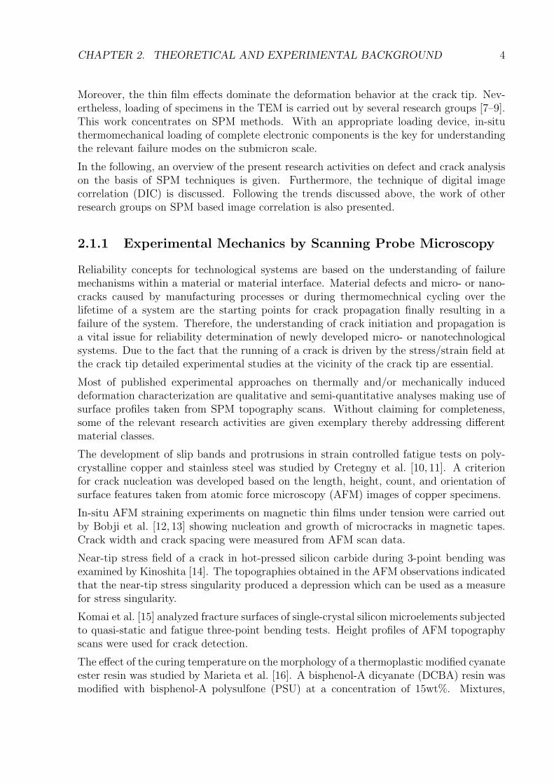
2.1.1 Experimental Mechanics by Scanning Probe Microscopy
Reliability concepts for technological systems are based on the understanding of failuremechanisms within a material or material interface. Material defects and micro- or nano-cracks caused by manufacturing processes or during thermomechnical cycling over thelifetime of a system are the starting points for crack propagation finally resulting in afailure of the system. Therefore, the understanding of crack initiation and propagation isa vital issue for reliability determination of newly developed micro- or nanotechnologicalsystems. Due to the fact that the running of a crack is driven by the stress/strain field atthe crack tip detailed experimental studies at the vicinity of the crack tip are essential.
Most of published experimental approaches on thermally and/or mechanically induceddeformation characterization are qualitative and semi-quantitative analyses making use ofsurface profiles taken from SPM topography scans. Without claiming for completeness,some of the relevant research activities are given exemplary thereby addressing differentmaterial classes.
The development of slip bands and protrusions in strain controlled fatigue tests on poly-crystalline copper and stainless steel was studied by Cretegny et al. [10, 11]. A criterionfor crack nucleation was developed based on the length, height, count, and orientation ofsurface features taken from atomic force microscopy (AFM) images of copper specimens.
In-situ AFM straining experiments on magnetic thin films under tension were carried outby Bobji et al. [12, 13] showing nucleation and growth of microcracks in magnetic tapes.Crack width and crack spacing were measured from AFM scan data.
Near-tip stress field of a crack in hot-pressed silicon carbide during 3-point bending wasexamined by Kinoshita [14]. The topographies obtained in the AFM observations indicatedthat the near-tip stress singularity produced a depression which can be used as a measurefor stress singularity.
Komai et al. [15] analyzed fracture surfaces of single-crystal silicon microelements subjectedto quasi-static and fatigue three-point bending tests. Height profiles of AFM topographyscans were used for crack detection.
The effect of the curing temperature on the morphology of a thermoplastic modified cyanateester resin was studied by Marieta et al. [16]. A bisphenol-A dicyanate (DCBA) resin wasmodified with bisphenol-A polysulfone (PSU) at a concentration of 15wt%. Mixtures,

CHAPTER 2. THEORETICAL AND EXPERIMENTAL BACKGROUND 5
postcured at the same conditions, were precured at various temperatures. Fracture sur-faces of three-point bending tests were analyzed by different SPM modes. Thermoplasticphases and the thermoset matrix were easily to be distinguished in images taken by fric-tion or phase mode. In another paper [17] Marieta et al. applied these imaging techniquesto a diglycidyl ether of bisphenol-A (DGEBA) epoxy matrix modified with polymethyl-methacrylate (PMMA) showing similar results.
Creuzet et al. [18] studied the fracture behavior of soda lime glass. The role of plasticity atthe crack tip is shown to demonstrate the need for a modification of the Griffith criterion.Intrinsic defects acting as stress concentrators could not be identified by AFM analysis.
An AFM analysis of the atomic structures of unloaded and loaded crack tips in the (001)surface of muscovite mica was carried out by Guan et al. [7]. A disorder zone with a widthof about 8nm ahead of a loaded crack tip was observed. Outside the disorder zone a normalelastic region was found. The question whether the dislocations emitted from the crack tipor not is not solved in the paper. Critical stress intensity factors are evaluated with theequation of Goken [19].
Crack tip blunting by dislocation emission and unstable crack propagation of NiAl singlecrystals in the AFM was studied by Goken et al. [19, 20]. NiAl serves as a model alloyfor the mechanical behavior of intermetallic compounds. A model of plastic crack openingdisplacement (COD) was used for fracture toughness evaluation, but the calculated valuesfor the stress intensity factor were not in good agreement with comparable measurementsof other research groups. The estimation by plastic COD generally led to lower valuesthan those obtained from load-displacement curves [20]. The depression in front of thecrack tip was also calculated on the basis of analytical equations and no good agreementwas found to AFM measurements. It was shown that three-dimensional FE calculationswere necessary [21]. Vehoff et al. [22] show that for single crystals dynamic computersimulations for the prediction of toughness do not agree with the measured toughness. Forthe measured slip plane length the simulations predict a much larger toughness.
In addition, Goken et al. [23] used optical interference microscopy (OIM) which has alarger lateral scale than AFM but a similar vertical resolution for measurements of thevertical depression at the crack tip. The results were compared to FEM calculations.Stress intensity factors were determined from the elastic displacements in vertical directionaround the crack tip. However a complete comparison and discussion of the FEM dataand the measurements is not published so far.
Parallel to the research at in-situ loading experiments, advanced SPM modes such asatomic force acoustic microscopy (AFAM) [24–26] and ultrasonic force microscopy (UFM)[27–30] are becoming powerful techniques for the determination of material properties onthe nanoscale.
Summarizing one can say that a satisfying model for the crack tip behavior in the veryvicinity of the crack tip is not available for most of the discussed material classes. Thereis a need for deformation measurement technique especially for crack tip analysis.

CHAPTER 2. THEORETICAL AND EXPERIMENTAL BACKGROUND 6
2.1.2 Micro Deformation Measurement Techniques
As discussed in the previous section, the determination of stress/strain fields at the cracktip is the key for a successful description of a failure mechanisms of a technological system.Thus, the measurement of stresses and strains at the surface of materials is a widely de-veloped field in material science. Today, a variety of deformation measurement techniquesare available, such as photoelasticity [31–34], Moire and speckle interferometry [35], stereoimaging techniques [36, 37] and digital image correlation [2, 38]. Most of these techniquesare highly specialized in specific research fields or make use of an extraordinary experimen-tal setup. The imaging techniques vary from video or CCD cameras, optical microscopy,white light microscopy, scanning electron microscopy (SEM), laser scanning microscopy(LSM) to scanning probe microscopy (SPM).
Nowadays, for the special case of microelectronic applications three methods of in-situmeasurement techniques are successfully employed by several research groups i.e. Moire,speckle techniques and digital image correlation. In the following, the principles of thesemethods are discussed the emphasize being laid on the method of digital image correlationwhich is the method of choice in this work.
Moire and Speckle Techniques
In the application of the Moire technique it has to be distinguished between geometric andinterferometric Moire. Geometric Moire is the intensity superposition phenomenon whentwo Ronchi gratings are superimposed whereas interferometric Moire is the amplitude andphase interference of two coherent light beams emanating from a diffraction grating on thespecimen surface. While the basic phenomena are different, the form of the resulting fieldequations are identical [39]. Both Moire methods resort to the deviation from a referencegrating pitch as a measure of deformation. If deformed gratings are superimposed withcorresponding reference gratings, Moire fringes result. With the knowledge of the gratingparameters displacement contours can be calculated from the fringes.
Matsumoto [40] originally proposed the use of Moire interferometry in 1972. But its de-velopment and application did not begin until the 80s and was initiated by Post [41]using optical Moire techniques. In the following, Moire methods were established in scan-ning electron microscopy [42, 43]. Today the development of the Moire method towardsnanometer resolution is carried out by Asundi and co-workers [35,44–46]. Gratings of 106
lines/mm are applied to generate AFM Moire. First applications were shown at integratedcircuit (IC) packages. Furthermore, the lattice of mica atoms is utilized as gratings fornano Moire measurements. The latest development is a deformation measurement Moireapproach based on focused ion beam (FIB) images [47].
Speckle methods utilize a random pattern of speckles to register deformation. Informationin terms of displacement is obtained through correlation between two speckle patterns. Itis sometimes referred to as the speckle Moire method, because the speckle pattern may beconsidered as a random grating with all orientations an a band limited spectrum of gratingpitch [48]. Through the process of optical (or digital) spatial filtering in form of Fourierdecomposition, an equivalent grating pitch with a specific orientation can be evaluated.
CHAPTER 2. THEORETICAL AND EXPERIMENTAL BACKGROUND 7
Regarding the speckle techniques it has to be distinguished between coherent [49] and in-coherent methods. Coherent speckle patterns results from the illumination of an opticallyrough surface with a coherent laser light whereas incoherent speckles are artificially pro-duced. For example, it can be created by spraying black paint from an aerosol onto a whitesurface.
Summarizing the application of Moire and Speckle techniques to actual questions of ma-terial research it can be concluded that their capability is also given for submicron mea-surements. However, due to the fact that digital image correlation techniques are easier tohandle they become a powerful deformation measurement technique.
Digital Image Correlation
The digital image correlation technique is a method of digital image processing. Digitizedimages of the analyzed objects in at least two or more different states (e.g. before and aftermechanical and/or thermal loading) have to be obtained with an appropriate imagingtechnique. Displacement fields are extracted by computer aided comparison of gray scaleimages (or image segments) by means of the application of a correlation algorithm.
Generally, correlation algorithms can be applied to images extracted from various sources.Digitized photographs or video sequences but also images from e.g. optical microscopy,SEM, LSM or SPM are suitable for the application of digital image correlation.
The method was introduced by Peters and Ranson [50] and Sutton et al. [38] who useddigital image correlation on laser speckle images. Improvements of the method were pub-lished in several papers [51–53]. By the application of stereo imaging an extension towardsthree-dimensional displacement fields was developed by Luo et al. [36].
During the last two decades digital image correlation methods were established by severalresearch groups. Examples from different fields of applications can be found in variouspublications, e.g. in [52–65]. Early attempts to acquire high resolution SEM images forsubsequent deformation analyses were made by Davidson [66] with the application of theso-called DISMAP system which allowed the digitizing of photographic micrographs. Inmodern SEM equipment however images are already ”captured” digitally so that corre-lation algorithms are applied directly to them. This approach has been chosen by var-ious research labs and is described in several publications [2, 37, 67–69]. In the groupof Michel the application of SEM images for deformation analysis on thermomechanicallyloaded electronics packages was established as the so-called microDAC method i.e. microDeformation Analysis by means of Correlation algorithms [2].
The latest development of the DIC methods is the extension towards nanometer scalemeasurements. The application of scanning probe microscopy for image acquisition is usedby the group of Knauss [64, 70–72] and Michel and co-workers [73–76] who named theirtechnique nanoDAC. Details will be discussed in Sect. 2.1.3.
The reason for the success of the DIC method, especially in the comparison to laser inter-ferometric or Moire methods, is based on several advantages:
• In many cases, only relatively simple low-cost hardware is required (optical mea-surements) or already existing microscopic tools like SEM and SPM can be utilizedwithout any changes.

CHAPTER 2. THEORETICAL AND EXPERIMENTAL BACKGROUND 8
• Once implemented in a well designed software code, the correlation analysis of grayscale images is user friendly and easy to understand in the measuring and post-processing process.
• For optical micrographs, no special preparation of the objects under investigationis needed at all. For low magnifications, required standards for the experimentalenvironment (e.g. vibration isolation, stability of environmental parameters like tem-perature) are not as high as in laser based measurements.
• The application and cumbersome preparation of object grids is not necessary.
• According to its nature the method possesses an excellent down-scaling capability.By using microscopic imaging principles, also very small objects can be investigated.
Therefore, correlation analysis of gray scale images is predestinated for qualitative andquantitative measurement of micro and nanomechanical properties.
2.1.3 The Combination of SPM Methods and Digital Image Cor-relation
The development of a deformation measurement technique based on scanning tunneling mi-croscopy (STM) and digital image correlation was introduced by the group of Knauss [77].For the measurements, a new STM system was designed to be coupled to a mechanicallydeforming specimen. Based on the two-dimensional DIC algorithm developed in the pub-lications of Sutton and Luo et al. [36,38,51,78] a modification of the DIC method towardsthree-dimensional deformation measurement was established [77]. Accuracy tests showthat an in-plane displacement error of ± 0.08 pixel or ± 2.4 nm and an out-of plane dis-placement error of ± 0.75 nm could be achieved by the STM-DIC method. On an STMimage of 10×10 µm the total possible in-plane displacement resolution of the technique was4.8 nm, whereas the total out-of plane displacement resolution was 1.5 nm [79]. STM-DICbased results were published on the deformation of a uniaxial stressed PVC specimen [70].The combination of atomic force microscopy and digital image correlation was developedby the research groups of Knauss and Michel. The first results were reported on cracktip field measurements of a thermoset material by Vogel and Michel [73, 80] followed by aarticle of Chasiotis and Knauss [64] on uniaxial tensile tests on polycrystalline silicon. Anoverview of the progress of the group of Knauss is given in [72].
From the above mentioned publications the following facts on AFM based digital imagecorrelation can be summarized:
• The AFM is a suitable image acquisition tool for the application of digital imagecorrelation. With the application of the AFM for micro- and nanomechanical de-formation analysis the foundation is laid for a detailed evaluation of the limits andpossible break down of continuum mechanics in the nanometer region.

CHAPTER 2. THEORETICAL AND EXPERIMENTAL BACKGROUND 9
• Problems encountered during data acquisition are the long scanning times hysteresisand creep effects of the piezo scanning tube. Nevertheless, new developments onscanning probe techniques and DIC software tools due to the demand in nanotechno-logy research will provide new measurement features enlarging the potential of theSPM based DIC analysis.
With the development of SPM-based DIC techniques, future failure and reliability problemson nanoscaled particles and material interfaces will be addressed. Thereby, the trendfrom micro electronic mechanical systems towards nano electronic mechanical systems issupported by an appropriate measurement technique.
2.2 The Method of Digital Image Correlation
The basic idea of the DIC algorithms results from the fact that images commonly allowto record local and unique object patterns within the more global object shape and struc-ture. These patterns are more or less stable if the objects are deformed by mechanical orthermal loads. Figure 2.1 and 2.2 show two examples of images taken by scanning electronmicroscopy and scanning force microscopy.
Markers indicate typical local pattern of the images. In most cases, these patterns areof stable appearance, even when severe load is applied to the specimens. In spite of thepresence of strong plastic, viscoelastic or visco-plastic material deformation, local patternscan be recognized after loading, i.e. they can function as a local digital marker for thecorrelation algorithm.
2.2.1 Cross Correlation Algorithms on Gray Scale Images
The cross correlation approach is the basis of the DIC technique. A scheme of the correla-tion principle is illustrated in Fig. 2.3. Images of the object are obtained at a reference loadstate 1 and at a different second load state 2. Both images are compared with each otherusing a cross correlation algorithm. In the image of load state 1 (reference) rectangularsearch structures (kernels) are defined around predefined grid nodes (Fig. 2.3, left). Thesegrid nodes represent the coordinates of the center of the kernels. The kernels themselvesact as gray scale pattern from load state image 1 that have to be tracked, recognized anddetermined by its position in the load state image 2. In the calculation step the kernel win-dow (n × n submatrix) is displaced inside the surrounding search window (search matrix)of the load state image 2 to find the best-match position (Fig. 2.3, right).
This position is determined by the maximum value of the cross correlation coefficient, K,which is calculated for all possible kernel displacements within the search matrix. Thecomputed cross correlation coefficient K compares gray scale intensity patterns of loadstate images 1 and 2. K is equal to

CHAPTER 2. THEORETICAL AND EXPERIMENTAL BACKGROUND 10
Figure 2.1. Appearance of local image structures (patterns) during specimen loading;SEM images of flip chip gold bump image size 100 × 100 µm; (left) at room temperature,(right) at 125 ◦C.
Figure 2.2. AFM topography image of a crack in a thermoset polymer material for dif-ferent crack opening displacements, scan size 15 × 15 µm.
Ki′,j′ =
i0+n−1∑i=i0
j0+n−1∑j=j0
(I1(i, j) − MI1) (I2(i + i′, j + j′) − MI2)√i0+n−1∑
i=i0
j0+n−1∑j=j0
(I1(i, j) − MI1)2
i0+n−1∑i=i0
j0+n−1∑j=j0
(I2(i + i′, j + j′) − MI2)2
(2.1)
where I1,2 and MI1,2 are the intensity gray values of the pixel (i, j) in the load stateimages 1 and 2 and the average gray value over the kernel size, respectively. The kerneldisplacement within the search matrix of load state image 2 is indicated by i′ and j′.Assuming quadrangle kernel and search matrix sizes Ki′,j′ values have to be determinedfor all displacements given by −(N − n)/2 ≤ i′, j′ ≤ (N − n)/2. The described searchalgorithm leads to a two-dimensional discrete field of correlation coefficients defined atinteger pixel coordinates (i′, j′). The discrete field maximum is interpreted as the location,where the reference matrix has to be shifted from the first to the second image to find the

CHAPTER 2. THEORETICAL AND EXPERIMENTAL BACKGROUND 11
' '
Figure 2.3. Displacement evaluation by cross correlation algorithm; (left) detail of areference image at load state 1; (right) detail of a image at load state 2; [81].
best matching pattern. Figure 2.4 shows an example of the correlation coefficients insidea predefined search window.
Figure 2.4. Discrete correlation function Ki′,j′ defined at integer (i′, j′) coordinates; themaximum of the coefficient of correlation is marked by an arrow [81].
With this calculated location of the best matching submatrix an integer value of the dis-placement vector is determined.

CHAPTER 2. THEORETICAL AND EXPERIMENTAL BACKGROUND 12
2.2.2 Subpixel Analysis for Enhanced Resolution
As described in the previous section, the cross correlation algorithm determines the dis-placements in the form of integer pixel coordinates. For the calculation of the displacementfield with a higher accuracy, the displacement evaluation has to be improved. Differentresearch groups [72, 73] reported the application of algorithms improving the accuracy ofthe cross correlation technique. In a second calculation step, special subpixel algorithmsare used to achieve higher displacement value resolution. The presumably simplest andfastest procedure to find a value for the non-integer subpixel part of the displacement isimplemented by parabolic fitting. The algorithm searches for the maximum of a parabolicapproximation of the discrete function of correlation coefficients in the close surroundingof the maximum coefficient Kmax,discrete. The approximation process is illustrated in Fig.2.5
Figure 2.5. Principle of the parabolic subpixel algorithm [81].
The location of the maximum of the parabolic function defines the subpixel part of thedisplacement. In most cases (on CCD camera and SEM images) this algorithm allows toget a subpixel accuracy of about 0.1 pixel. With more advanced algorithms accuracies ofup to 0.01-0.02 pixel for common 8 bit digitized images are possible [81]. However, it hasto be stated that the overall accuracy depends on the image source, signal noise, stabilityduring image caption and on the contrast of the pixels of the correlation kernel to a largeextent.
2.2.3 Results of Digital Image Correlation
The results of the two-dimensional cross correlation and subpixel analysis in the surround-ings of a measuring point primarily are the two components of the displacement vector.

CHAPTER 2. THEORETICAL AND EXPERIMENTAL BACKGROUND 13
Applied to a set of measuring points (e.g. to a rectangular grid of points with user de-fined pitches), this method allows to extract a complete in-plane displacement field. In thesimplest way the results can be displayed as a numerical list which can be post-processedusing standard scientific software codes. Commonly, graphical representations such as vec-tor plots, superimposed virtual deformation grids or color scale coded displacement plotsare implemented in commercially available or in in-house software packages. Figure 2.6shows two typical examples of graphical presentations of the results at an AFM image.
Figure 2.6. Digital image correlation results derived from AFM images of a crack tip,scan size 15 × 15 µm; (left) Image overlaid with user defined measurement grid and vec-tor plot of displacements; (right) Image overlaid with user defined measurement grid anddeformed measurement grid; (displacement vector and deformed grid presentation are en-larged with regard to the image magnification).
Finally, taking numerically derivatives of the obtained displacement fields ux(x, y) anduy(x, y) the in-plane strain components ε and the local rotation angle ρ are determined:
εxx =∂ux
∂x, εyy =
∂uy
∂y, εxy =
1
2
(∂ux
∂x+
∂uy
∂y
), ρxy =
1
2
(∂ux
∂x− ∂uy
∂y
)(2.2)
Derivation is included in some of the available correlation software codes or can be per-formed subsequently with the help of mathematical software packages.
2.2.4 Accuracy
The accuracy of the displacement measurement is defined by the imaged area dimensionsat the object in horizontal x- and vertical y-direction, lx,y, the pixel resolution of the imagein x- and y-direction, mx,y and the subpixel shift resolution k. It is given by, [81]:
δux,y = (lx,y/mx,y)k (2.3)

CHAPTER 2. THEORETICAL AND EXPERIMENTAL BACKGROUND 14
The subpixel shift resolution k is a measure for the available displacement resolution andstrongly depends on the experimental conditions, the quality of the images obtained inthe experiment (e.g. noise, sharpness of pixel information) and the quality of the appliedsoftware algorithms. The value for k varies in most of the relevant cases between 1/4to 1/100 pixel [81]. For calculation results obtained by statistical evaluation of multiplepoint measurements (e.g. rigid body displacement calculated as the mean value of shiftsmeasured at multiple points, linear elastic strain calculated from the slope of a regressionline) resolution equivalents to 0.01 pixel and better are reached, although the correlationsoftware itself does not provide this level of accuracy. Assuming values of a SPM largescale scan size of lx, ly = 50 µm, a scan resolution mx,my = 512 and a measurable subpixelshift k = 0.2 (estimated), a measurement resolution of a single one-point displacementvalue down to 20 nm can be obtained with scanning probe microscope applications (Eqn.2.3). With a scansize of 2.5 µm, a resolution of 1 nm is a realistic value.
2.3 Fracture Mechanics Approach
From a macroscopic, continuum mechanics point of view a crack is defined as infinitelysharp and is, therefore, a geometric singularity. The loading of a crack can be applied bythree different modes, as illustrated in Fig. 2.7.
Mode I Mode IIIMode II
crack front
crack surfacecrack face
x
z
y
Figure 2.7. Principle loading modes that can be applied to a crack.
In mode I, the load is applied normal to crack plane introducing a symmetric separationof the upper and lower crack surfaces. Mode II can be described as in-plane shear loadingand mode III as out-of plane shear. The crack can be loaded in one of these modesor in a mixture of two or three modes. In an actual application, especially at a crackof a microelectronic component, these modes are difficult to separate from each other.Moreover, the mode type may change during a single load cycle, over service time orduring crack growth.
For the linear elastic fracture mechanics approach (LEFM) on the basis of continuummechanics the size of the process zone is of great significance. The process zone is the region

CHAPTER 2. THEORETICAL AND EXPERIMENTAL BACKGROUND 15
in the vicinity of the crack front (2D: crack tip) were micro or nanoscopically small damageand reordering processes prevail. Metals, for example, deform plastically which causes cracktip blunting. The occurring yielding process is dominated by dislocation motion along slipplanes. Polymers, however, have a different microscopic fracture behavior. Depending onthe molecular structure of the polymer chain scission, disentanglement of polymer chains,shear yielding and crazing are dominating processes at the highly stressed crack tip (adetailed discussion on polymer fracture is given in Sect. 3.1). Nevertheless, the behavior ofthe process zone cannot be described by continuum mechanics theory. For the consistentdescription of the stress state by LEFM it has to be assumed that the process zone issufficiently small compared to the macroscopic geometry of the cracked body.
Fundamental for understanding fracture behavior of a cracked body is the crack tip fieldi.e. the stress-strain field in the surrounding of the crack tip. Especially in the area ofmicroelectronics where the dimensions of functional and passive layers or other componentsare becoming smaller with every newly developed process technology the understanding ofthe deformation field around a defect or crack is of primary interest.
Therefore, the crack tip field of a cracked body with isotropic and linear elastic materialbehavior under static load will be addressed in the following section.
2.3.1 Crack Tip Field Analysis
A two-dimensional body with a straight crack as illustrated in Fig. 2.8 can be analyzedassuming a plane strain or plane stress configuration. For the mathematical derivationof the crack field it is convenient to introduce a polar coordinate system (r, θ) with itsorigin at the crack tip. The derived stress/strain field description can be transferred tocartesian coordinates (x,y) by coordinate transformation. For this case the stresses at anarea element is defined as illustrated in Fig. 2.8.
crackx
y
τxy
τyx
σxx
σyy
θr
Figure 2.8. Body with through-thickness crack; definition of coordinate axes in cartesiancoordinate system (x,y).
A specific crack tip loading according to the defined modes produces a 1/√
r stress singular-ity at the crack tip with a mode depended stress intensity factor, K. Thus the asymptoticstress fields at a crack tip can be written as [82]:

CHAPTER 2. THEORETICAL AND EXPERIMENTAL BACKGROUND 16
limr→0
σ(n)ij =
Kn√2πr
f(n)ij (θ) (2.4)
where Kn describes the stress intensity factors according to the relevant loading mode n (I,II or III), and fij is a dimensionless function. For mode I crack opening the displacementfield at the crack tip is described by:
ux =KI
2µ
√r
2πcos
θ
2
(κ − 1 + 2 sin2 θ
2
)(2.5)
uy =KI
2µ
√r
2πsin
θ
2
(κ + 1 − 2 cos2 θ
2
)(2.6)
where µ is the shear modulus of the material and κ is defined as
κ = 3 − 4ν
κ = (3 − ν)/(1 + ν)
for plane strain, and
for plane stress,
(2.7)
(2.8)
where ν is the Poisson’s ratio.
In most of the practical cases of a cracked body, the three-dimensional description of thefracture problem is necessary. In general, a curved crack front has to be treated in a three-dimensional manner. Examples are penny-shaped inner crack problems or semi-ellipticalsurface cracks. An exact description of a crack with a straight crack front in a plate offinite thickness also requires a three-dimensional analysis because the state of stress variesalong the z-coordinate of the crack front (compare to Sect. 4.3).
2.3.2 K-Concept
Fundamentals
We consider the most relevant crack loading configuration which is the pure mode I crackopening. As described in the previous section, the crack tip field is characterized by thestress intensity factor KI . However Eqn. 2.4 leads to an infinite stress value if the distancefrom the crack tip, r, reduces to 0. Real materials do not withstand infinite stress. Metalsrespond with the formation of a plasticity zone where polymers show crazing in order toachieve a relaxation of the stresses. The K-concept is only valid if the size of that inelasticregion in the surrounding of the crack tip is sufficiently small. Then the K-dominated arealies within an inner radius, rp, and an outer radius, R as illustrated in Fig. 2.9.
Outside the radius R higher order terms of the stress solution have to be taken into account.The inner bound of the K-dominate zone is given by rp where the increasing stressescause plastic deformation. Described in a more general term, the material reacts with aninelastic deformation compared to the elastic deformation (linear elasticity theory) of theK-dominated zone, [83].

CHAPTER 2. THEORETICAL AND EXPERIMENTAL BACKGROUND 17
r
R
rpρ
K-dominated zoneplastic zone
Figure 2.9. Crack tip behavior under the assumption of the K-concept [83].
With the assumption that the region of the inelastic and process zone (indicated by theradius ρ) is small compared to the K-dominated zone (ρ, rp � R) the behavior at the cracktip can be described by the K-factor. This is the underlying theory of the K-concept. Thestress intensity factor allows the definition of a fracture criterion: The crack extensionoccurs if a material dependent critical stress intensity factor, Kc, prevails at the crack tip.The critical stress intensity factor is called the fracture toughness. It is a material propertyand, therefore, independent of the geometry of the specimen or structure.
Measurement of K-Factor
For the measurement of the stress intensity factor the singularity at the crack tip of atest specimen have to be equivalent to the underlying theoretical approach. Most of theclosed-form K solutions directly derived from stress functions are only valid for cracks ininfinite plates. For usual test specimens with finite dimensions and crack sizes similar tothe boundary geometries of the specimen closed-form solutions are not available. However,the influence of the geometry on the stress field can be corrected by appropriate geometryfunctions.
In this work the standardized CT-specimen (CT: compact tension) corresponding to ASTM5045, [84], was used for the experimental fracture tests. The CT-specimen and the nomen-clature of the geometry parameters are illustrated in Fig. 2.10.
The stress intensity factor for the CT-specimen is defined by:
KI =F
B√
Wf(α) (2.9)
where F is the applied load and f is the geometry function of the non-dimensional cracklength, α, with α = a/W
f(α) =2 + (α)
(1 − α)3/2=[0.866 + 4.64(α) − 13.32(α)2 + 14.72(α)3 − 5.6(α)4
](2.10)
The specimens have to be prepared with a pre-crack initiated by a cyclic loading (typicallyused for metals) or tapping of a razor blade (for brittle polymers). The thickness, B, of the

CHAPTER 2. THEORETICAL AND EXPERIMENTAL BACKGROUND 18
a
F
W
B
1.25 x W
0.25 x W
1.2 x W
0.55 x W
F
Figure 2.10. CT-specimen with geometry according to ASTM D5045 [84].
specimen have to be sufficiently large to ensure a state of plane strain over a sufficientlylarge portion of thickness B.
2.3.3 Energy Release Rate
Irwin [85] has introduced the concept of energy release rate G which is the available energydW for an increment of crack extension dA:
G = −dΠ
dA(2.11)
G is the change of potential energy Π with the crack area A during crack extension. Theenergy release rate is a measure for the crack tip load and the tendency of crack extension. Itis the basis for numerical determination of fracture mechanical properties utilizing fracturemechanical integral concepts developed by Rice [86].
In case of a through crack in an infinite plate subjected to a tensile stress and linear elasticmaterial behavior the energy release rate can related to the stress intensity factor through:
G =K2
I
E(2.12)
For plane strain configurations E have to be replaced by E/(1 − ν2).

CHAPTER 2. THEORETICAL AND EXPERIMENTAL BACKGROUND 19
F
F
A
dA
F
Displacement
dW = -dΠ
A+dA
A
W
Π
Figure 2.11. Energy release rate.
2.4 Numerical Fracture Mechanics Utilizing Integral
Concepts
Besides the K-factor and the energy release rate G the J-integral is another parameterdescribing the fracture behavior of a material. For linear elastic fracture mechanics G andJ are equivalent and K can be determined from G or J . Despite the K- and G-conceptthe J-integral is also valid for inelastic material behavior.
The J-integral was proposed by Rice [86] and is defined by:
J =
∫Γ
(wdy − Ti
∂ui
∂xds
)(2.13)
where Γ is a counter-clockwise path around the crack tip, w is the strain energy density,Ti are components of the traction vector and ds is a length increment of the contour Γ.The strain energy density is defined by
w =
εij∫0
σijdεij (2.14)
where σij and εij are the stress and strain tensors, respectively, and the components of thetraction vector are given by
Ti = σijnj (2.15)
where nj are the components of the unit vector normal to Γ.

CHAPTER 2. THEORETICAL AND EXPERIMENTAL BACKGROUND 20
Another advantage of the J-integral is its invariant behavior according to the chosen con-tour around a crack tip, so that a relatively coarse mesh can be used in finite elementbased simulations. With the assumption of elastic material behavior the J-integral can berelated to the K-concept by the equation:
J =1
E(K2
I + K2II) +
1
2µK2
III (2.16)
where E is the Young’s modulus and µ is the shear modulus.
For the numerical calculation of the J-integral different methods were developed. Parks [87]and Hellen [88] suggested a virtual crack extension method which is based on a stiffnessderivative formulation of selected elements surrounding the crack tip. The problem of thismethod is that the calculation involves cumbersome numerical differencing. Moreover, itis not suited to problems including thermal strain [82].
Another definition of the J-integral which is excellently suited for FEA was proposed byde Lorenzi [89,90]:
J = −dΠ
dA=
1
δA
∫V
[(σij(Fjk − δjk) − wδik)
∂∆xk
∂xi
]dV (2.17)
where δA is an increase in the crack area generated by a virtual crack advance, V is thevolume of the body, Fjk are the body forces, δjk Kronecker’s delta and ∆xk is a mappingfunction which maps the body containing the crack into a body with a slightly increasedcrack length.
Figure 2.11 illustrates an incremental virtual crack extension. In a three-dimensional prob-lem the J-integral may vary along the crack front (compare to Sect. 4.3).
The application of the J-integral as defined in Eqn. 2.13 is limited to elastic or plasticbehavior, the deformation has to be monotone and cyclic loading is not allowed. For thedescription of inelastic material behavior (plasticity, creep) several integral concepts weredeveloped. Table 2.1 summarizes the most important integral concepts for experimen-tal material characterization and FE-based fracture mechanical problems on the field ofmicroelectronics.
The C� integral is defined by replacing strains of Eqn. 2.13 with strain rates, and dis-placements with displacement rates, where w is the stress work rate (power) density. TheC� parameter is only valid for crack growth in the presence of global steady state creep.Materials with a sufficiently slow crack growth compared to growing creep zones spreadingout throughout the specimen can be characterized by C� [82].
Ghavifekr [91] proposed the generalized J-integral proposing a separation between elasticand inelastic (plastic, creep and thermal) components of the deformation gradient. Theidea of this type of integral is the assumption that the crack can only be driven by anelastic process and only elastic energy can be released during crack propagation.

CHAPTER 2. THEORETICAL AND EXPERIMENTAL BACKGROUND 21
Table 2.1. Advanced integral concepts
Concept Integral Material
C�
[92, 93]
C�1 =
∫Γ
(wdy − Ti
∂ui
∂xds)
w =˙εkl∫
0
σijd ˙εij
viscoplastic
Goldman,Hutchinson,
Landes, Begley 1975
J
[94]
J1 =∫Γ
ti∂ui
∂X1ds − ∫
ν
σij∂ui,j
∂X1dν plastic, viscoplastic
Kishimoto, AokiSakata 1980
∆T �
[95, 96]
∆T � =∫
S−S0
[∆Wn1 − (ti + ∆ti)∆ui,1 − ∆tiui,1] ds
+∫
V −V0
[∆σij(εij,1 + 1
2∆εij,1)
]dν
− ∫V −V0
[∆εij(σij,1 + 1
2∆σij,1)
]dν
plastic, viscoplastic
Atluri 1983
The generalized J-integral is given by
JG = −dΠ
dA=
1
δA
∫V
[(σij(F
El.jk − δjk) − wEl.δik)
∂∆xk
∂xi
]dV (2.18)
where only the elastic energy and the elastic deformation is considered in the calculationof the JG-integral.

Chapter 3
Testing and Results
The experimental approach to nanostructured materials and components is the key forsuccessful design of microelectronic devices of the future. Therefore, well established mea-surement techniques for the determination of material properties have to be combinedwith new highly specialized strategies. Macroscopic material properties determined frommeasurements at bulk materials are becoming more and more ineffective for FE-basedprediction of life-time and system reliability.
In the following chapter, material testing by standard testing procedures and a newly devel-oped deformation measurement technique on the micro to nanoscale will be discussed. Theresults are presented in correspondence with the applied testing techniques and methods.
Section 3.1 gives an introduction to the chosen polymeric material system which is employedas a model material for the experimental approaches. In Sect. 3.2 the viscoelastic materialcharacterization is shortly described together with the obtained material description. Themain emphasis of this chapter is laid on newly developed experimental methods which werethe motivation of this work. Namely, the development and application of the nanoDACmethod for micro- and nanoscaled deformation measurement (Sect. 3.4) and the researchon the Optical Crack Tracing (OCT) system providing an advanced measurement techniquefor fracture mechanical parameters of polymers (Sect. 3.3) are discussed.
3.1 Polymeric Materials
3.1.1 Mechanical Behavior of Polymeric Materials
The mechanical behavior of polymers depends on various characteristic properties, such asthe degree of polymerization, molecular weight, polydispersity, and the molecular structure.These measures can be controlled by production process parameters (time, temperature)and by added catalysts, compatibilizers, etc.
The possible molecular structures of the polymer chains which have a significant influenceon the mechanical properties are illustrated in Fig. 3.1. Thermoplastic polymers consist oflinear and branched chains. Typically, the polymer chains in an elastomer are organized inlightly cross-linked structures and are, therefore, capable to withstand large elastic strains.
22
CHAPTER 3. TESTING AND RESULTS 23
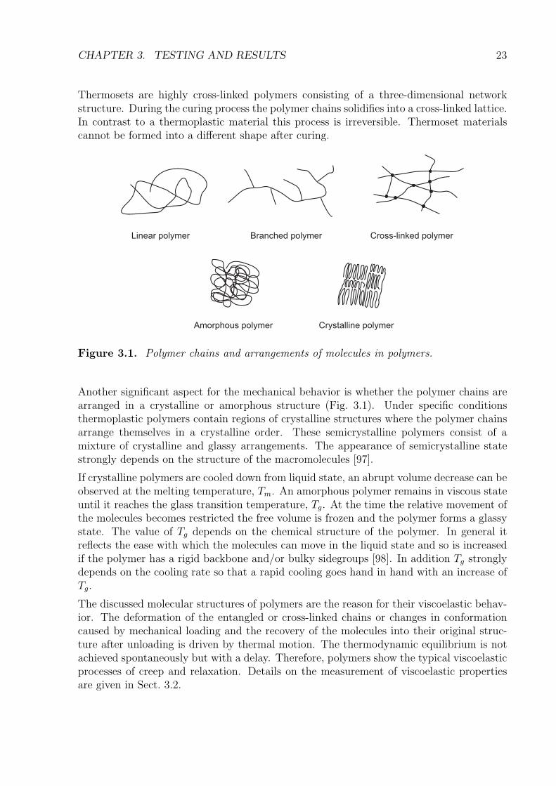
Thermosets are highly cross-linked polymers consisting of a three-dimensional networkstructure. During the curing process the polymer chains solidifies into a cross-linked lattice.In contrast to a thermoplastic material this process is irreversible. Thermoset materialscannot be formed into a different shape after curing.
Linear polymer Branched polymer Cross-linked polymer
Amorphous polymer Crystalline polymer
Figure 3.1. Polymer chains and arrangements of molecules in polymers.
Another significant aspect for the mechanical behavior is whether the polymer chains arearranged in a crystalline or amorphous structure (Fig. 3.1). Under specific conditionsthermoplastic polymers contain regions of crystalline structures where the polymer chainsarrange themselves in a crystalline order. These semicrystalline polymers consist of amixture of crystalline and glassy arrangements. The appearance of semicrystalline statestrongly depends on the structure of the macromolecules [97].
If crystalline polymers are cooled down from liquid state, an abrupt volume decrease can beobserved at the melting temperature, Tm. An amorphous polymer remains in viscous stateuntil it reaches the glass transition temperature, Tg. At the time the relative movement ofthe molecules becomes restricted the free volume is frozen and the polymer forms a glassystate. The value of Tg depends on the chemical structure of the polymer. In general itreflects the ease with which the molecules can move in the liquid state and so is increasedif the polymer has a rigid backbone and/or bulky sidegroups [98]. In addition Tg stronglydepends on the cooling rate so that a rapid cooling goes hand in hand with an increase ofTg.
The discussed molecular structures of polymers are the reason for their viscoelastic behav-ior. The deformation of the entangled or cross-linked chains or changes in conformationcaused by mechanical loading and the recovery of the molecules into their original struc-ture after unloading is driven by thermal motion. The thermodynamic equilibrium is notachieved spontaneously but with a delay. Therefore, polymers show the typical viscoelasticprocesses of creep and relaxation. Details on the measurement of viscoelastic propertiesare given in Sect. 3.2.

CHAPTER 3. TESTING AND RESULTS 24
The fracture process of polymer is primarily dominated by two types of bonds i.e. covalentbonds between atoms of the molecular chain and secondary van der Waals forces betweenmolecule segments. Secondary bonding forces act between adjacent molecules or segmentsof the same (folded) molecule. For the formation of new surfaces during the fractureprocess the covalent bonds have to break. Nevertheless, the van der Waals forces play asignificant role during the deformation process before the ultimate fracture. The factorsthat govern the toughness and ductility of polymers include strain rate, temperature, andmolecular structure. At high loading rates or low temperatures (relative to Tg) polymersshow a brittle behavior, because there is insufficient time for the material to respond tostress with large-scale viscoelastic deformation or yielding. Highly cross-linked polymersare also incapable of large scale viscoelastic deformation [82]. For cross-linked polymers vander Waals forces are not significantly involved in the fracture process. For these materialsbreakage of primary bonds is necessary to enable large scale deformations.
Especially for ductile polymers plastic deformation is dominated by the following mecha-nisms:
1. Shear yielding: This is a large scale deformation at constant volume leading to apermanent change in specimen shape. The formation of shear bands is possible atspecific strain rates and temperatures. Shear yielding is activated by a translation ofmolecules past each other when a critical shear stress is reached. In semicrystallinepolymers it takes place through slip, twinning and martensitic transformation. Inglassy polymers highly localized shear bands or diffuse shear deformation zones areformed [98].
2. Crazing: Glassy polymers subjected to tensile loading often yield by crazing, whichis a highly localized deformation that leads to cavitation (void formation) and strainson the order of 100 % [82]. In contrast to shear yielding crazing is accompaniedby a change (increase) in specimen volume. Crazes are generally nucleated at im-perfections in polymer specimens such as surface flaws or dust particles. Multiplecrazing can lead to general yielding and act as a toughening mechanism in polymers.Polymers with a second phase are specially prepared to take the advantage of thistoughening mechanism [98].
Crazing and shear yielding are competing mechanisms; the dominating behavior dependson molecular structure, stress state and temperature [82].
An increase of toughness of a material can be achieved by enlarging the deformation ability.This task is related to realization of higher strength and strain values.
Increase of material strength can be obtained by [99]:
• Decrease of regions of local stress concentration to minimize the tendency of micro-crack initiation. Therefore, highly homogeneous materials are necessary requiringcost-intensive production processes.

CHAPTER 3. TESTING AND RESULTS 25
• Increase of local strength by orientation of macromolecules. This concept is realizedin fibers, liquid-crystal polymers and fiber reinforced polymers. However, the draw-back of such materials is the requirement of special production processes and theanisotropy of the material with poor strength values perpendicular to the orientationdirection.
• Rapid fluctuation of local stress concentrations by relaxation in order to minimizethe tendency for crack formation. This requires local areas of high molecular mobilityin the immediate neighborhood of stress concentrations or microcracks to guarantystress relaxation or crack arrest. The described concept requires the application ofheterogeneous multiphase polymer systems.
Increase of strain can be realized by [99]:
• Decrease of yield stress by increasing molecular mobility. This concept is known assoftening which goes hand in hand with a decrease in strength.
• Realization of numerous local (microscopic) yield regions achievable by an appropri-ate material heterogenization.
The last statement implies that processes of local energy absorption have to take place insuch a large volume of polymer material that the required energy absorption can be realized.Possible energy absorbing processes are small scale yielding, plastic zone formation, crazing,shear yielding or molecule chain scission [99].
Nevertheless, it has to be noted that an increase of a specific mechanical property oftenhas an influence on other properties. The price for an increase in fracture toughness oftengoes to a decrease in mechanical module.
3.1.2 Cyanate Ester Thermosets
In the past, the growing demand for high performance, high temperature resistant, andeasy-to-process matrix resins in fibre-reinforced composites and electronic applications hasencouraged research on several thermosetting polymeric materials. The most significantgroup is the epoxy resins which are broadly used among other fields of applications instructural parts of aerospace vehicles and for encapsulant material and IC-board matrixmaterial of electronics industry. For higher service temperatures epoxies cannot be usedand other candidates such as cyanate ester resins have to be investigated to fulfil thisrole [100].
A comparison of conventional high performance thermoset matrix resins with cyanate esterresins (CE) is given in Fig. 3.2.
Developments in molecular architecture have produced second generation cyanate esterresins with performance in the Tg range 190-290◦C with inherently more toughness thaneither epoxies or bismaleimides (BMI), lower moisture absorption and lower dielectric-lossproperties [100].

CHAPTER 3. TESTING AND RESULTS 26
300
200
100
400
0 2 3 4 5 6 7
DICYANATE
DIEPOXIDE
BMI
TETRA-
EPOXIDE
T [°C
]
Tensile Strain at Break [%]
1
PMR
TOUGHEND
BMI
P-T
g
Figure 3.2. Relationship of Tg and tensile strain-at-break for several families of commer-cial thermoset resins [101].
The chemical composition of a cyanate ester monomer is given in Fig. 3.3 containing thereactive ring-forming cyanate (–O–C≡N) functional groups. Chemically this family ofthermosetting monomers and their prepolymers are esters of bisphenols and cyanic acid.The R in the structural model of Fig. 3.3 may be a range of functional groups, e.g. hydrogenatoms, methyl or allyl groups, and the bridging group may be simply an isopropylidenylmoiety or an extended aromatic or cycloaliphatic backbone etc. [100].
Cyanate ester monomers polymerize by a cyclotrimerization reaction to a cyanurate linkednetwork polymer. A description of this step-growth reaction would go beyond the scope ofthis work. Details can be found in various publications [3, 102].
Cyanate esters comprise the properties of high thermal stability, low outgassing, and radi-ation resistance [103], low dielectric constant (2.5− 3.1), dimensional stability at solderingtemperatures (Tg: 250-290◦C) and low moisture absorption 0.6 − 2.5% with the process-ability of epoxy resins. These properties make cyanate ester resins a material of choice forhigh speed printed circuit boards. An encapsulant material for bare mounted chips wasformulated by blending of AroCy L-10 with RTX-366 (both of them are CEs) [101]. Asnap cure application for electronic packaging on the basis of a combination of CE andencapsulated hardener particles was reported by Bauer [104]. The single largest use for
X
R R
R R
OO NN C C
Figure 3.3. General structure of commercial cyanate ester monomers.

CHAPTER 3. TESTING AND RESULTS 27
RO
ON
N
NN
RO
O
N
N
O
O
R
Figure 3.4. Structure after cyclotrimerization.
CEs is the lamination of substrates for printed circuits and their assembly via prepreg ad-hesives into high density, high speed multi-layer boards [105]. High frequency circuits forwireless communication and tracking systems with frequencies up to 12 GHz are the fastestgrowing use [101]. Fast growing application of CEs are dispatcher radios, pagers, cellularphones, global positioning, satellite broadcast, and radar tracking systems. Cyanate es-ters are likely to find applications in photonics, as optical wave guides, and in nonlinearoptics [106,107].
Besides, electronics CEs are also applied in aerospace applications where their advantages incomparison to other resins are predominating factors and cost is only of secondary concern.Primary and secondary structures in military aircraft, radome and satellite applicationsare important fields of application. Low out-gassing, minimal dimensional changes duringthermal cycling, good long term stability, self adherent properties to honeycomb and foamcores, good electrical properties and high service temperatures are the key advantages fortheir applications in aerospace [101].
A drawback of highly cross-linked thermosets, such as cyanate esters, is their brittlenessand low impact resistance. Although a cured cyanate resin has a relatively high toughnesscompared to a cured BMI or a crosslinked epoxy resin, it still requires suitable modifica-tion to improve toughness without reducing the intrinsic physical strength for structuralapplications. The uncured cyanate resins are compatible with a number of amorphousthermoplastic polymers, including copolyester, polysulfones, polyether sulfones, polyacry-lates and polyether imides [16]. In the course of curing, most of the mentioned poly-mers phase-separate into micron or sub-micron sized domains exhibiting a co-continuousor phase-inverted morphology at concentrations > 15wt% because of the high molecularweight of the thermoplastic [106].
Kinloch and Taylor [108] report on toughening of CEs with polyether sulfone (PES) whichcan increase the fracture energy of up to 800 %. In current research the application ofnanofillers is becoming a promising approach. Ganguli et al. [109] developed nanocompos-
CHAPTER 3. TESTING AND RESULTS 28
ites by dispersing organically modified layered silicates (OLS) into a cyanate ester resin.With an inclusion of 5% by weight the modulus and the toughness was increased by 30 %.
3.1.3 Tested Material Systems
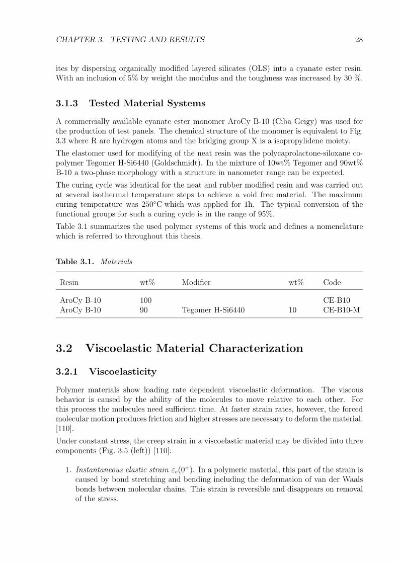
A commercially available cyanate ester monomer AroCy B-10 (Ciba Geigy) was used forthe production of test panels. The chemical structure of the monomer is equivalent to Fig.3.3 where R are hydrogen atoms and the bridging group X is a isopropylidene moiety.
The elastomer used for modifying of the neat resin was the polycaprolactone-siloxane co-polymer Tegomer H-Si6440 (Goldschmidt). In the mixture of 10wt% Tegomer and 90wt%B-10 a two-phase morphology with a structure in nanometer range can be expected.
The curing cycle was identical for the neat and rubber modified resin and was carried outat several isothermal temperature steps to achieve a void free material. The maximumcuring temperature was 250◦C which was applied for 1h. The typical conversion of thefunctional groups for such a curing cycle is in the range of 95%.
Table 3.1 summarizes the used polymer systems of this work and defines a nomenclaturewhich is referred to throughout this thesis.
Table 3.1. Materials
Resin wt% Modifier wt% Code
AroCy B-10 100 CE-B10AroCy B-10 90 Tegomer H-Si6440 10 CE-B10-M
3.2 Viscoelastic Material Characterization
3.2.1 Viscoelasticity
Polymer materials show loading rate dependent viscoelastic deformation. The viscousbehavior is caused by the ability of the molecules to move relative to each other. Forthis process the molecules need sufficient time. At faster strain rates, however, the forcedmolecular motion produces friction and higher stresses are necessary to deform the material,[110].
Under constant stress, the creep strain in a viscoelastic material may be divided into threecomponents (Fig. 3.5 (left)) [110]:
1. Instantaneous elastic strain εe(0+). In a polymeric material, this part of the strain is
caused by bond stretching and bending including the deformation of van der Waalsbonds between molecular chains. This strain is reversible and disappears on removalof the stress.

CHAPTER 3. TESTING AND RESULTS 29
2. Delayed elastic strain εd(t). The rate of increase of this part of strain decreasessteadily with time. It is also elastic, but, after removal of the load, it requires timefor complete recovery. In a polymeric material, the delayed elastic strain is caused,for instance, by chain uncoiling.
3. Viscous flow εv(t). It is an irreversible component of strain which may or may notincrease linearly with time of stress application. In a polymeric material it is causedby interchain slipping.
Phenomenologically, two aspects of viscoelastic behavior can be observed i.e. creep responseunder a constant stress and stress-relaxation response under constant strain.
A linear viscoelastic material have to meet two conditions: proportional stress/strain be-havior and superposition of subsequent loading regimes is possible. Figure 3.5 (right)illustrates the principle of superposition.
σ
t
σ(t)
σ1
σ2
∆ε 1
τ 2τ 1
ε
∆ε 2
tt 1
σ
t
σ0
Loading
Unloading
σ = σ0
σ = 0
0
ε
t
ε (t ) + ε (t )1 1d v
ε (0 ) +e
ε (t-t )1R
Figure 3.5. Viscoelasticity; (left) Creep and recovery of a viscoelastic specimen subjectedto a constant stress until time t1; (right) Superposition of stresses, σ, caused by twoHeaviside step functions in strain ε1 and ε2.
The response to single straining steps can be superposed to form the solution σ(t). For acontinuous description the constitutive equation is given by:
σ(t) =
t∫−∞
E(t − t′)ε(t′)dt′ (3.1)
The creep and relaxation function are related via the integral:
t∫−∞
E(t − t′)D(t′)dt′ = t (3.2)

CHAPTER 3. TESTING AND RESULTS 30
The relaxation modulus, E(t) and the creep compliance, D(t) fully describe the time-dependent response of viscoelastic materials. For the measurement of viscoelastic behavioreither the relaxation modulus or the creep compliance can be derived from tensile testswith fixed strain or stress, respectively:
E(t) =σ(t)
ε0
D(t) =ε(t)
σ0
(3.3)
3.2.2 Modeling of Viscoelasticity
The physical representation of a viscoelastic material is commonly established by a com-bination of spring/dashpot models [110]. The basis are Maxwell elements with a springand a Newtonian dashpot in series and Kelvin-Voigt elements with a parallel arrange-ment of spring and dashpot. A generalization of the material model can be defined by acombination of several Kelvin-Voigt and/or Maxwell elements. Due to the fact that theexperimental derivation of the viscoelastic behavior was carried out by stress relaxationexperiments, in the following the emphasis is laid on the description by Maxwell elements.This leads to a straightforward approach for the functional description of the relaxationfunction as illustrated in Fig. 3.6. Details on other modelling approaches can be found invarious textbooks on polymer mechanics [97,110,111].
σ
E1 E2 EN.....
η1 η2 ηN
σ
Figure 3.6. Generalized Maxwell model for viscoelastic material.
All of these N Maxwell elements are described by the differential equation:
σ + τ σ = ηε (3.4)
where η is the fluid viscosity in the dashpot element and τ = η/E is the relaxation time.The solution of this differential equation is the relaxation function:

CHAPTER 3. TESTING AND RESULTS 31
E(t) = E exp(− t
τ) (3.5)
The relaxation function of the generalized system of parallel Maxwell elements is given bythe Prony series:
E(t) =N∑
i=1
Ei(t) =N∑
i=1
Ei exp(− t
τi
) (3.6)
For the numerical implementation of viscoelastic material properties usually Prony seriesas given by Eqn. 3.6 are implemented in available FE codes, so that the stress-relaxationis described by a series of exponential functions with experimentally fitted parameters.
3.2.3 Time-Temperature-Superposition
In the mechanical behavior of polymer materials an equivalence in the material reaction toloading at high temperatures and after long time intervals was found. This was the basisfor Williams, Landel and Ferry [112] developing a semi-empirical equation which allows theshifting of relaxation curves measured at different temperatures to a single modulus-timemaster curve. They defined the shift factor, aT as:
log aT = logtTtT0
=C1(T − T0)
C2 + T − T0
(3.7)
where tT and tT0 are times to reach a specific modulus at temperatures T and T0, whereT0 is a reference temperature (usually defined at the glass transition temperature, Tg), andC1 and C2 are material fitting parameters. Time-temperature-superposition is the basisfor straightforward material characterization by simple stress relaxation test at various(sufficient) temperatures.
3.2.4 Experimental Setup and Data Acquisition
The measurement of the viscoelastic material properties was carried out through stressrelaxation tests at specified temperatures. A standard testing machine (Zwick Z 1446)equipped with a temperature chamber was used for the measurements. The chosen speci-mens were ”dogbone” shape specimens according to DIN 53504 [113]. The specimens weremachined as defined by the geometry S3A (overall length of the specimen: 50 mm, parallellength: 16 mm, thickness: 2 mm). During loading the strain was measured direct at thespecimen surface using Zwick’s universal extensometer ”Multisens”. The load was appliedwith a velocity of 5 mm/min until a strain value of 0.2 % was reached. Then, the crossheadof the machine was stopped and a stress relaxation test i.e. force measurement was carriedout for one hour. The relaxation tests were only carried out at the temperatures of 25 and150◦C . Due to the fact that the loading experiments of Sect. 3.4.4 are carried out in ap-proximately one hour these two temperatures are sufficient for the viscoelastic descriptionof the polymer material.

CHAPTER 3. TESTING AND RESULTS 32
3.2.5 Results of Viscoelastic Material Characterization
Figure 3.7 shows the results of the neat CE in a logarithmic plot, including the fittedmaster curve. The master curve has to be understood as fitting function of the relaxationcurve. A complete material characterization ranging over large time/temperature regimewas not necessary in this work.
-1 0 1 2 3 4 5 6 7 8 9 10
1600
1800
2000
2200
2400
2600
2800
3000
� � �� �� � ��� ��� � ��� ��
� � �� �� ���� ��� � �
� � �����
�������
���
���� ������
Figure 3.7. Master stress-relaxation curve of cyanate ester resin.
The fitted Prony series of the cyanate ester resin is given by:
E = 2070 + 100 et
1010 + 100 et
109 + 50 et
108 + 60 et
107 + 50 et
106
+60 et
105 + 60 et
104 + 80 et
103 + 90 et
102 + 70 et10 + 50 et [MPa]
(3.8)
The Prony-type description of viscoelastic material is suited for the application in finiteelement software. FE calculations of Sect. 4.4 refer to the material model given by Eqn.3.8.
3.3 Advanced Fracture Analysis for Polymers
The group of Bauer developed the Optical Crack Tracing (OCT) system which is a tech-nique of automatic determination of fracture toughness, KIc, by means of optical crack tip

CHAPTER 3. TESTING AND RESULTS 33
localization [114,115]. The system allows the measurement of the R-curve, i.e. the fracturetoughness for crack initiation and propagation. With the measurement of the R-curveinstead of the fracture toughness according to the standard ASTM D5045 [84] a betterunderstanding of the fracture behavior is achieved. The benefits of the OCT method canbe summarized as follows:
• Information on the type of crack propagation such as steady state, stick-slip andintermediate between steady state and stick-slip can be extracted.
• The influence of time dependent phenomena on the fracture behavior of polymerscan be analyzed.
• Prevention of overestimation of fracture toughness induced by non-ideal pre-cracksis established.
In the following, a short description of the system the measurement principle and theextracted results are given. A detailed discussion of the technique can be found in thepapers of Uhlig, Kahle, Keller and Bauer et al. [114–116].
3.3.1 Optical Crack Tracing (OCT) Technique
The Optical Crack Tracing system (LaVision OCT) includes hardware and software compo-nents to record crack length at the beginning and during crack propagation by video record-ing and subsequent digital image analysis. The set-up of the system is shown schematicallyin Fig. 3.8.
Figure 3.8. Scheme illustrating the experimental set-up of OCT.
During the fracture test the video images and the force signal from the testing machine arestored in the RAM of a personal computer. After the test the series of images is analyzed byimage analysis software. Digital filter algorithms filter the maximum gradient in brightnessand by subsequent setting of brightness threshold other structures in the image are removed

CHAPTER 3. TESTING AND RESULTS 34
Figure 3.9. Image before and after image analysis used for crack length determination;(left) original image showing a brightness gradient at the crack face; (right) filtered imageshowing the structures with maximum brightness gradient values.
so that only the crack is retained. An example of such an image analysis is shown in Fig.3.9.
A step gradient in brightness of the crack is achieved by lightening the specimen at aninclined angle. This technique can be applied to transparent and non-transparent materi-als. In the case of a non-transparent material a 10-bit CCD camera with a resolution of1024×768 pixel should be used to achieve optimized brightness gradients at the crack face.The analysis software identifies the crack by segment routines (the longest segment foundis identified as the crack) and the crack tip location is determined in pixel coordinates.A scaling procedure which utilizes markings (compare to Fig. 3.9 (left)) on the specimentransforms the pixel coordinates directly into crack length data. By simultaneously mea-suring the load/displacement curve and crack-length/displacement curve the OCT softwarecalculates the stress intensity factor KI from relationships known for standard geometriesof crack test specimen (Eqns. 2.9, 2.10). A typical set of measured data and results isshown in Figs. 3.10 and 3.11.
0.0 0.1 0.2 0.3 0.4 0.5 0.60
20
40
60
80
Load [N
]
Loading Pin Displacement δ [mm]
0.0 0.1 0.2 0.3 0.4 0.5 0.610
15
20
25
30
35
Cra
ck L
en
gth
a [
mm
]
Loading Pin Displacement δ [mm]
Figure 3.10. Example for a typical set of load vs. displacement and crack length vs. dis-placement diagrams measured by Optical Crack Tracing.
In the following, the merits of measuring the R-curve rather than calculating only the ini-tiation fracture toughness from the load at fracture and the initial crack length (measured

CHAPTER 3. TESTING AND RESULTS 35
15 20 25 30 350.2
0.3
0.4
0.5
0.6
0.7
0.8
KI [
MP
am1
/2]
Crack Length a [mm]
Figure 3.11. Results of the fracture mechanical analysis: R-curve (KI , at crack initiationand propagation).
by analyzing the crack front as is described in the standards) shall be discussed.
3.3.2 Measurement of the R-curve in Comparison to StandardASTM D5045
The typical case of an R-curve for stable fracture which can be described by linear elasticfracture mechanics is shown Fig. 3.11. In this example, the fracture toughness is thesame for crack initiation and propagation, which can be expected for the case of linearelastic fracture mechanics. The procedure described in the A.S.T.M standard [84], whichcalculates only a single value for crack initiation and the measurement of the R-curve wouldlead to identical values.
However, the standard for the determination of crack initiation fracture toughness requiresan ideal pre-crack, i.e. an initial crack that is ideally sharp and lies in the plane of symmetryof the specimen. This so-called self-similar crack cannot be guaranteed by the usualmethod of tapping in a sharp razor blade to generate a pre-crack.
Non-ideal pre-cracks are cracks which lead to an increase of crack initiation stress intensityfactor i.e. the fracture toughness. In the cases where the crack front is not parallel to theplane of symmetry because it is twisted or there are steps in the pre-crack front a significantincrease of the crack initiation stress intensity factor is found. Under this conditions thecrack opening mode I is superposed by mode II behavior (compare to Sect. 2.3) inducinga higher resistance to fracture than a pure mode I crack opening.
Accurate quantitative analysis by mapping the fracture surfaces of a large number ofspecimens confirmed the visual observation. As an example, the analysis of the cracksurface of a specimen with a step-like initial crack front is shown in Fig. 3.12. To analyze

CHAPTER 3. TESTING AND RESULTS 36
the influence of the step height ∆y is introduced as illustrated in Fig. 3.12. The value ofstep height ∆y is decreasing during crack propagation until a plane crack front is formed.
z
y
xy
z
y
Figure 3.12. (left) CT-specimen with non-ideal pre-crack; (right) topographical (y)-map of crack surface; note: the x-coordinate at the axis is not identical to the crack lengtha of the CT-specimen.
In Fig. 3.13 the effect of a non-ideal pre-crack on the R-curve is illustrated. The criticalstress intensity factor and the step height ∆y as defined in Fig. 3.12 are plotted vs. thecrack length.
0
100
200
300
15 20 25 30 350.0
0.4
0.5
0.6
0.7
KI [M
Pam
1/2]
Crack Length a [mm]
∆y [µ
m]
Figure 3.13. R-curve and step height ∆y vs. crack length.

CHAPTER 3. TESTING AND RESULTS 37
The shape of the R-curve at the beginning of the crack propagation can be easily under-stood because in the case of a step-like crack front there is also a mode II component in-cluded and the fracture toughness in mode II is significantly higher than that in mode I. Bythe same argument it can be understood that the crack approaches the plane of symmetryduring crack propagation and consequently fracture toughness approaches the true modeI value for the material as can be seen in Fig. 3.13. Thus in cases of non-ideal pre-cracksstill the true mode I fracture toughness can be obtained if the R-curve is measured [117].
3.3.3 Results of OCT
The measured R-curve of the neat cyanate ester resin and the rubber modified resin systemis shown in Fig. 3.14. The results clearly show the effect of the rubber modification on thefracture behavior. On the one hand the fracture toughness is increased from 0.5 to a valueof 0.9 MPam1/2, on the other hand the fracture occurs in a stick-slip type.
0.2 0.4 0.6 0.8 10.2
0.4
0.6
0.8
1
1.2
Str
ess
Inte
nsity
Fac
tor
[MP
am1/
2 ]
Normalized Crack Length a/W
CE-B10CE-B10-M
Figure 3.14. R-curve of unmodified and rubber modified cyanate ester resin.

CHAPTER 3. TESTING AND RESULTS 38
Table 3.2. Fracture toughness and Young’s modulus
Material E [MPa ] KIc [MPam1/2]
CE-B10 2800 0.5CE-B10-M 2700 0.9
From the obtained results from OCT based fracture toughness testing the following ques-tions arise:
• Does the stick-slip behavior correlate with micro- or nanoscopic morphology of theneat and rubber modified polymers (process zone)?
• Does crack tip blunting prevail in the process zone of the rubber modified system?
In Sect. 4.3 Fig. 4.4 an example of stick-slip behavior is illustrated by fractographicalmicroscopy image.
3.4 Crack Field Analysis by In-Situ AFM Measure-
ments - nanoDAC
The measurement and evaluation of deformation processes on the micro- and nanoscopicrange by the combination of SPM equipment and the technique of digital image correlationis a task requiring special prerequisites on the technical equipment. Three main issues haveto be discussed if digital image correlation is supposed to be applied on SPM data:
• suitable specimen loading devices must be designed or adapted to the SPM equip-ment,
• high level scanning stability and reproducibility have to be provided,
• concepts for correction of scanner drifts have to be developed.
Following these objectives the utilized apparatus and arisen stability problems and theirsolution have to be discussed.
3.4.1 General Aspects of Scanning Probe Microscopy
With the development of the scanning tunneling microscope (STM) [118] and the atomicforce microscope (AFM) [119] the foundation was laid for fundamental and technologyorientated research on the nanoscale. Nowadays, the development of new scanning probemicroscopy (SPM) techniques is a vital task for the nanotechnology driven product de-velopment. SPMs have been developed for various applications. These include – STM,

CHAPTER 3. TESTING AND RESULTS 39
AFM, friction (or lateral) force microscopy (FFM or LFM), scanning electrostatic forcemicroscopy (SEFM), scanning force acoustic microscopy (SFAM) (or atomic force acousticmicroscopy (AFAM)), scanning magnetic microscopy (SMM) (or magnetic force microscopy(MFM)), scanning near field optical microscopy (SNOM), scanning thermal microscopy(SThM), scanning electrochemical microscopy (SEcM), scanning Kelvin Probe microscopy(SKPM), scanning chemical potential microscopy (SCPM), scanning ion conductance mi-croscopy (SICM), and scanning capacitance microscopy (SCM). A good starting point forfurther reading and related papers on this SPM techniques is the ”Handbook of Nano-technology”, [120].
A complete description of the various techniques would be beyond the scope of this thesis.Therefore, only the significant details of the applied SPM instruments and the utilizedimaging techniques are discussed in the following.
The AFM used in this work (ThermoMicroscopes (VEECO), Autoprobe M5) is designedas illustrated in Fig. 3.15.
PZT
ScannerTube
Position-Sensitive
Photodetector
Feedback Loop
Sample (fixed)
Laser
Adjustable
Mirror
Cantilever
Figure 3.15. Principle of AFM.
The drive of the cantilever in the scanning- (x, y) and height- (z) direction is achievedby a piezoceramic tube scanner (100 × 100 µm large area scanning unit). The heightinformation of the scanned surface is picked up by a so-called beam bounce detection system[121]. A laser beam is reflected from the back of the cantilever onto a position-sensitivephotodetector (PSPD) via an adjustable mirror. As the cantilever bends the position ofthe laser spot on the PSPD changes resulting in a voltage shift which is a measure forthe cantilever deflection. With the feedback-loop the scanning tube is adjusted to theactual height of the surface, so that a constant deflection of the cantilever is guaranteedduring scanning. For atomic flat surfaces the system can also be driven in constant heightmode where the cantilever is held at a constant height and the variation of the cantilever

CHAPTER 3. TESTING AND RESULTS 40
deflection is recorded. The signal for the drive of the scanner tube in z-direction is callederror-signal. It is derived from the difference of the last to the actual value of the PSPD.
The usage of piezoceramics as scanning units for the x- and y-directions have the disad-vantage of high nonlinearities in the behavior of the applied voltage to the resulting strainof the PZT material. Therefore, the so-called scan master which can be understood asa linearization matrix enables correct positioning of the cantilever [121]. Due to the factthat piezoceramics also show time dependent material properties calibration routines inx, y and z-direction have to be carried out from time to time.
The AFM can be used either in a static or dynamic mode. In the static mode, also knownas repulsive mode or contact mode the cantilever tip is brought in contact with a samplesurface. During contact, the cantilever experiences a very weak (repulsive) force causedby the electronic orbital overlap of the atoms at the end of the tip with the atoms in thesample surface. The force acting on the tip causes a cantilever deflection which is measuredby the PSPD. In the dynamic mode of operation for the AFM, also referred to as attractiveforce imaging or noncontact imaging mode, the tip is brought in close proximity (within afew nm) to the sample so that very weak van der Waals attractive forces are present at thetip-sample interface. The cantilever is vibrated either in amplitude modulation [122] modeor frequency modulation [123] mode. In contact mode, the interaction force between tipand sample is measured by measuring the cantilever deflection. In noncontact mode, theforce gradient is obtained by vibrating the cantilever and measuring the shift of resonantfrequency or the change of vibration amplitude.
To obtain topographic information of the scanned surface, the interaction force is eitherrecorded direct, or used as a control parameter for a feedback loop that maintains the forceor force derivative at a constant value [120]. To overcome the limitations of contact mode(influence of friction on topographic image) and to analyze the surfaces of soft materials theAFM can also be operated in the so-called tapping mode [124]. In this cantilever vibratesclose to its resonance frequency and the tip lightly taps the surface rather than getting intocontact with fully repulsive interaction. In addition to topographic imaging the tappingmode can also be used for the analysis of surface mechanical properties. Generally, the tip-sample interaction causes a change in the amplitude, the phase and the resonance frequencyof the vibrating cantilever. The spatial variation of these changes can be presented ininteraction (amplitude, phase or frequency shift) images [125].
3.4.2 Instrumentation of AFM measurements
The installation of thermal and/or mechanical loading stages in the SPM is mainly a ques-tion of compact design of loading stages, free access for SPM cantilevers to the specimenand a probe actuation instead of a specimen actuation. The available SPM equipment(Autoprobe M5) and loading stages required the installation of additional spacers betweenthe scanning head and the ground plate. The tension/compression loading device as illus-trated in Fig. 3.16 is attached to x-y-stages with positioning accuracies of ± 10 nm in onedirection and ± 1 nm in the other direction. In addition, fine adjustment in the nanometerrange can also be performed by the piezo drive of the AFM. In order to minimize scanninginstabilities and different thermomechanical drifts (compare to Sect. 3.4.3) common tools

CHAPTER 3. TESTING AND RESULTS 41
of environmental isolation are installed. This comprises active vibration compensation ofequipment tables and acoustic enclosures against ambient sound.
The employed tension/compression testing module is designed for in-situ SEM and SPMmeasurements (Fig. 3.16). For the case of the crack tip deformation field measurements atCT-specimens the module is equipped with a pin holder. For tension/compression tests onstandard tension specimens micro-vices are available in various configurations. In additionstandard tension/compression specimens can be thermally loaded with a contact heatingsystem which is placed under the specimen. Figure 3.16 shows the module with an insertedCT-specimen, where Fig. 3.17 shows the set-up of the loading device with the CT-specimenunder the SPM scanning head as it is installed during SPM measurements.
Figure 3.16. Tensile module with CT-specimen.
3.4.3 Stability Aspects of SPM Measurements
In comparison to DIC-based measurements treating optical or SEM images, some moreessential difficulties have to be overcome for SPM-based imaging. They relate to theextreme magnification of SPM techniques. Since SPM image scans are taken over a timeinterval from one to several minutes, even minor system drifts can cause significant artificialobject deformations. Classifying different drift sources it can be distinguished between:
• SPM scanner drifts, which are related to time dependent behavior of the piezo tube,
• relative movements between the scanning head and the sample fixture, mainly causedby temperature changes,
• drift of sample loading parameters (temperature, forces, load paths, etc.) withintesting stages installed at the microscope, and

CHAPTER 3. TESTING AND RESULTS 42
scanning head
loading device
SPM optics
CT specimen
cantilever carrier chip
Figure 3.17. In-situ loading of CT-specimen under SPM.
• incremental object deformations originating from viscoelastic material behavior oftest specimens, i.e. time dependent object deformations which take place even underconstant loading parameters.
Substantial concerns regarding stability and reproducibility originate from drifts of theSPM scanner piezo and the variation of thermomechanical loading parameters over time.As a consequence, the accurate selection of SPM equipment and loading stages is a crucialissue. Moreover, the development and implementation of methods of drift control andcompensation may be essential for particular applications.
In practical operation serious problems arise from the fact that the drift effects describedabove are not evident from a single image achieved at a specific load state of the specimen.In some cases severe drift effects come to light by digital image correlation of several imagesacquired at the same load state. For example, significant pseudo displacements occur whenthe scanner is adjusted to a new position of its scanning range either by the zooming-incapability of the SPM control software or user based definition of the new scanning rangeor scanning position. The application of DIC to images taken just after such positioningprocesses show large pseudo displacements caused by scanner creep. In some cases, thisartifact is visible at a single image without the aid of a DIC analysis. The initial part ofthe scan range of a test pattern would appear distorted as illustrated in Fig. 3.18.
An example of the creep effect, with a pseudo strain in the vertical y-direction being clearlyvisible without the application of the DIC method is given in Fig. 3.19.
The images show a region of 15 × 15 µm of an unloaded and stable mounted object witha metallic surface where the fast scanning is in the horizontal direction and the y-direction

CHAPTER 3. TESTING AND RESULTS 43
Figure 3.18. After a region of a sample is scanned with the AFM it is common to zoominto a small section of the image to get a higher magnification of an image. Scanner driftwill cause the image to appear distorted at the beginning of the scan [126].
is scanned from top to bottom. The images are taken in noncontact mode and the data isextracted from one scan direction only to suppress artifacts caused by scanner hysteresis.The images are acquired directly after each other using the repeat function of the SPMsoftware. The black polyline added to the topography images has the same size and positionin both images but the particle marked with an arrow is not in the same position relativeto the polyline. This implies a straining of the second (right) image relative to the first(left) image which should result in a large pseudo-strain if DIC method is applied to theseimages.
Figure 3.19. Two scans of a steel surface directly after repositioning of scanning range;the pseudo strain of the image at the right hand side compared the other image is visibleby the different location of the particle marked with an arrow; image properties: 15 × 15µm, 256 × 256 pixel, z-range: 213 nm.
To underline the creep effect of the scanner, a DIC displacement analysis is performed onthe images of Fig. 3.19. In this case, only the y-direction of the displacement vector isof interest and the determined results are shown together with the image source in Fig.3.20. The displacement results are given in pixel coordinates (1 pixel ≈ 59 nm). The first

CHAPTER 3. TESTING AND RESULTS 44
conclusion is that there is a general drift of several pixels across the vertical dimensionof the image. Secondly the displacement results clearly imply that there are larger strainvalues in the upper half of the image than in the lower half. This pseudo-strain effect iscaused by the creep behavior of the piezo scanner. After a running-in phase it will convergeinto steady state scanning behavior. As a result the pseudo-strain mainly occurs in theupper part of the image.
Figure 3.20. Pseudo displacements in vertical direction uy in [pixel], caused by scannercreep; contour lines of identical displacement are closer to each other indicating a largerstrain level in the upper part of the image.
The presented example emphasizes the requirements of stable scanning behavior to avoidartificial object deformation. As mentioned above, another important aspect is the thermaldrifts of the apparatus including the AFM itself but also the specimen, loading device andits positioning system. Moreover, these different drift sources superpose so they canceleach other out or enlarge each other depending on the actual environmental and systemimmanent influences. Attempts about correcting the displacement by eliminating onespecific stability source will always end up in the problem of the separation of the differentsources.
Therefore, a feasible strategy would be the estimation of the actual drifts of the completesystem in their summation rather than separating a single drift source. One possibleway to follow this objective is the description of the drift by a functional and applying a

CHAPTER 3. TESTING AND RESULTS 45
linearization to achieve an actual value for the system drift for a specific time period. Apracticable way to determine the actual system drift would be to capture a series of 2-3images at each of the load states to be compared. By a subsequent displacement analysis ofeach series utilizing the DIC code a mean drift value for each load state can be determined.If there is a difference between the mean drift at the specific load states, a correction has tobe applied to the obtained DIC results between these load states. The described strategycan be tested by a series of scans on a fixed specimen. In the following, these test will becalled ”zero displacement test”.
The displacements and their standard deviation determined from a zero displacement testare also a measure for the accuracy of the DIC concept on SPM images. According to [81]the applied DIC code has a pixel resolution of 0.1 for in-plane displacement componentsfor CCD camera images. Assuming that the code performs similar on AFM topographs,a displacement resolution of 0.2 nm is to be expected for a 1 × 1 µm scan and an imageof 512 × 512 pixel (Eqn. 2.3). In practical operation, it is difficult to translate displacea macroscopic specimen with that accuracy. However, a zero displacement test and theresulting variation of the displacement is a measure for the precision of the measurements.
In the following section these zero displacement tests are discussed. Nevertheless, it hasto be mentioned that new or somehow configured SPM and loading equipment should betested for stability and accuracy. The presented results can only give a system descriptionof the actual utilized equipment within this work. The trend of the SPM manufacturerto develop scanning equipment with increased line scan frequency can be very helpful tominimize the thermal and creep induced drift. Furthermore the application of closed-loopscanners comprising a positioning control unit will compensate scanning reproducibilityproblems.
Zero Displacement Tests
The zero displacement tests were performed by 256 × 256 pixel scans on a Ni-layer onsilicon substrate with scans sizes of 10 and 2 µm and a line frequency of 1 Hz. The fastscan direction was the horizontal x-direction and noncontact topography data was picked-up in the positive x-direction only in order to eliminate scanner hysteresis effects. Thescans were carried out in a series of 15 images using the ”repeat” option of the AFMcontrol software, so that non-stop scanning was performed for approximately 1 h on eachspecimen.
Figure 3.21 gives an impression of the observed system drifts for the sequence of the2 × 2 µm scans. The particle-like feature marked with an arrow clearly shows the prevailingdrift over the image series.
A quantification of the drift can be easily performed by DIC techniques. The image se-quences are analyzed by means of digital image correlation with each image being comparedto the subsequent one. From the determined displacement fields the following statisticalvalues are extracted:
1. Mean system drift determination over scan-time.

CHAPTER 3. TESTING AND RESULTS 46
t = 0s t = 266s t =532s
t =798s t =3722s
No. 1 No. 2
No. 4
No. 3
No. 15...............
Figure 3.21. Sequence of ”zero displacement test” for a 2× 2 µm scan; z-range: 47 nm.
2. Standard deviation of measured displacement in fast (x) and slow (y) scan direction.
The results of the analysis are presented in Figs. 3.22-3.25 where the evaluation of the meandisplacement and standard deviation was carried out separately for the x- and y-direction.Mean displacement values of the analyzed image series over scanning time (Figs. 3.22and 3.23) clearly emphasize that system drifts can be described with simple polynomialfunctions. The data was polynomial fitted with a degree of 4 where the graphs of the fittedfunctions are also shown. The extrapolation from 2 or 3 initial mean drifts to a subsequentimage can be achieved with the obtained fitting function. With the calculated mean drifta strain component across the whole image can be calculated so that a pseudo-strain canbe eliminated from the actual displacement measurements.
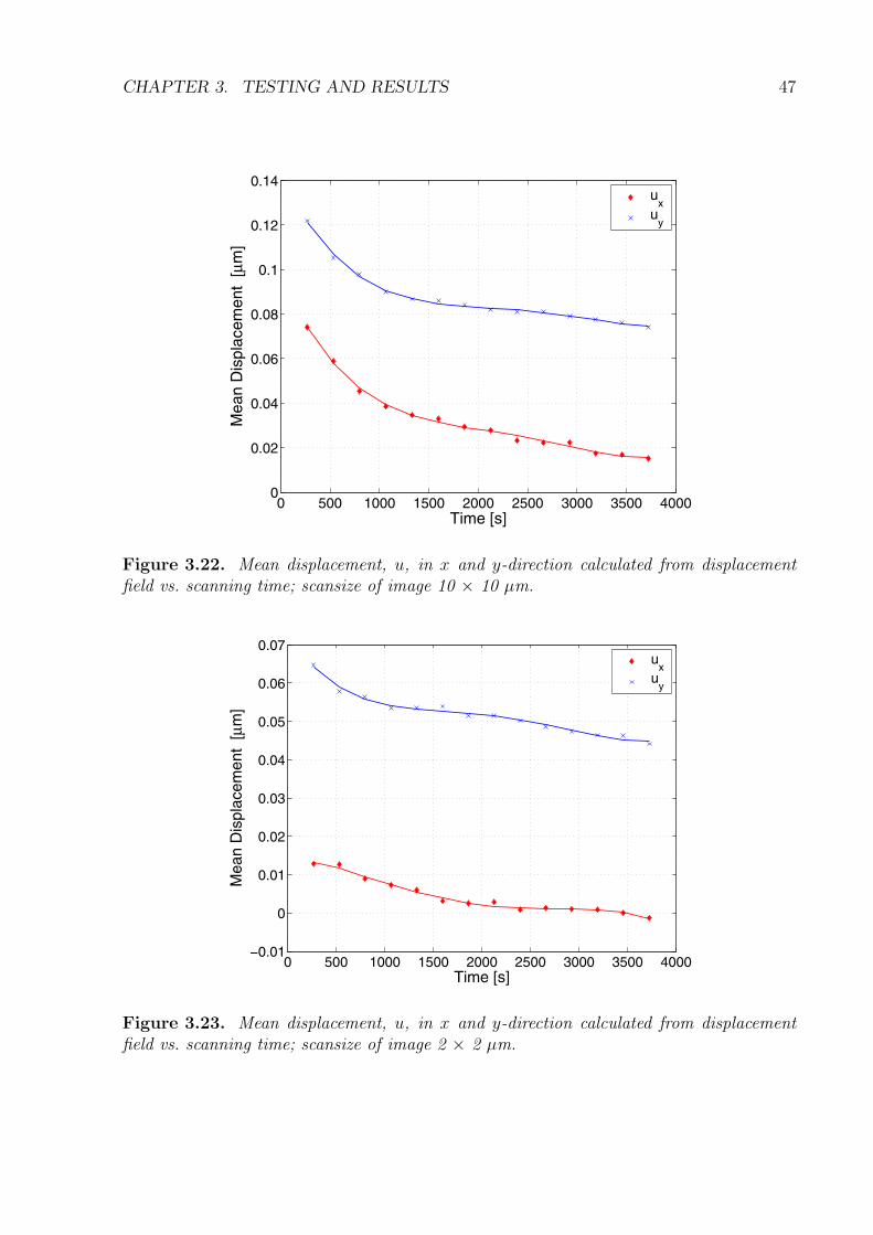
CHAPTER 3. TESTING AND RESULTS 47
0 500 1000 1500 2000 2500 3000 3500 40000
0.02
0.04
0.06
0.08
0.1
0.12
0.14
Time [s]
Mea
n D
ispl
acem
ent
[µm
]
ux
uy
Figure 3.22. Mean displacement, u, in x and y-direction calculated from displacementfield vs. scanning time; scansize of image 10 × 10 µm.
0 500 1000 1500 2000 2500 3000 3500 4000−0.01
0
0.01
0.02
0.03
0.04
0.05
0.06
0.07
Time [s]
Mea
n D
ispl
acem
ent
[µm
]
ux
uy
Figure 3.23. Mean displacement, u, in x and y-direction calculated from displacementfield vs. scanning time; scansize of image 2 × 2 µm.

CHAPTER 3. TESTING AND RESULTS 48
0 500 1000 1500 2000 2500 3000 3500 40000
1
2
3
4
5
6
7
8x 10
−3
Time [s]
Sta
ndar
d D
evia
tion
[µm
]
x−directiony−direction
Figure 3.24. Standard deviation of u in x and y-direction calculated from displacementfield vs. scanning time; scansize of image 10 × 10 µm.
0 500 1000 1500 2000 2500 3000 3500 40000
1
2
3
4
5
6
7
8x 10
−3
Time [s]
Sta
ndar
d D
evia
tion
[µm
]
x−directiony−direction
Figure 3.25. Standard deviation of u in x and y-direction calculated from displacementfield vs. scanning time; scansize of image 2 × 2 µm.

CHAPTER 3. TESTING AND RESULTS 49
The standard deviation calculation of the determined displacement values was also carriedout separately for the x- and y-direction. Figure 3.24 shows that the relative error at thebeginning of the 10 × 10 µm zero displacement test is in the range of ± 7.5 nm for the y-and ± 2.5 nm for the x-direction. This is caused by creep effects of the piezo scanner andthermal instabilities. After 5 scans the error is minimized to ± 1 nm for both directions.The outlying values at ≈ 530 s and ≈ 2400 s are caused by somewhat obscure scanninginstabilities which cannot be explained. For the 2 × 2 µm zero displacement tests (Fig.3.25) the standard deviation has already decreased down to ± 1 nm after 2 scans. Forlonger scanning times the error stabilizes between ± 0.25 and ± 1 nm.
The discussed results of the error analysis have to be compared to the general accuracyof the DIC analysis. The resolution of DIC for 10 × 10 µm scans with 256 × 256 pixel is7.8 nm as calculated by Eqn. 2.3. Zero displacement tests, however, reveal better resultsso that the value of k for this case of AFM images can be set to a value lower than 0.2(compare to Sect. 2.2.4). However, it has to be noted that the value for k strongly dependson the experimental conditions (noise, image contrast, ...).
The presented results and the discussion lead to the following statements for system driftevaluation and compensation:
• By the application of the DIC analysis it is possible to quantify system drifts duringin-situ loading tests.
• A system drift compensation can be done using the results from the drift analysis.
• Standard deviation values below 1 nm for a scan size of 2× 2 µm show that pseudo-deformation effects due to scanner instabilities are smaller than the DIC-softwareresolution.
Alternative AFM Modes for the Application of DIC
For the application of digital image correlation it can be more effective to use imagesbased on error signal or phase detection rather than topography. The error signal isdescribed in Sect. 3.4.1. The advantage of error images is the higher contrast for smallscan sizes where ”small” strongly depends on the surface roughness and on the signal noisewhich is responsible for the quality of the image. Within this work, the mechanicallypolished surfaces have a typical roughness of 15 nm average roughness Ra. The noise ofthe topography image is typically in the range of several A. Below 1 µm the error imagesmay give better results for the digital image correlation. A qualified analysis of error imagebased image correlation is not carried out in this work. Rather than error images, here theemphasis is laid on phase detection microcopy images and their application to DIC. Theadvantage of the phase signal compared to the topography signal is the additional materialstiffness contrast information which is the result of the interaction between the vibratingtip and the specimen surface (compare to Sect. 3.4.1). As for the error images the contrastof a phase image can be better suited for the application of DIC than the correspondingtopography image.
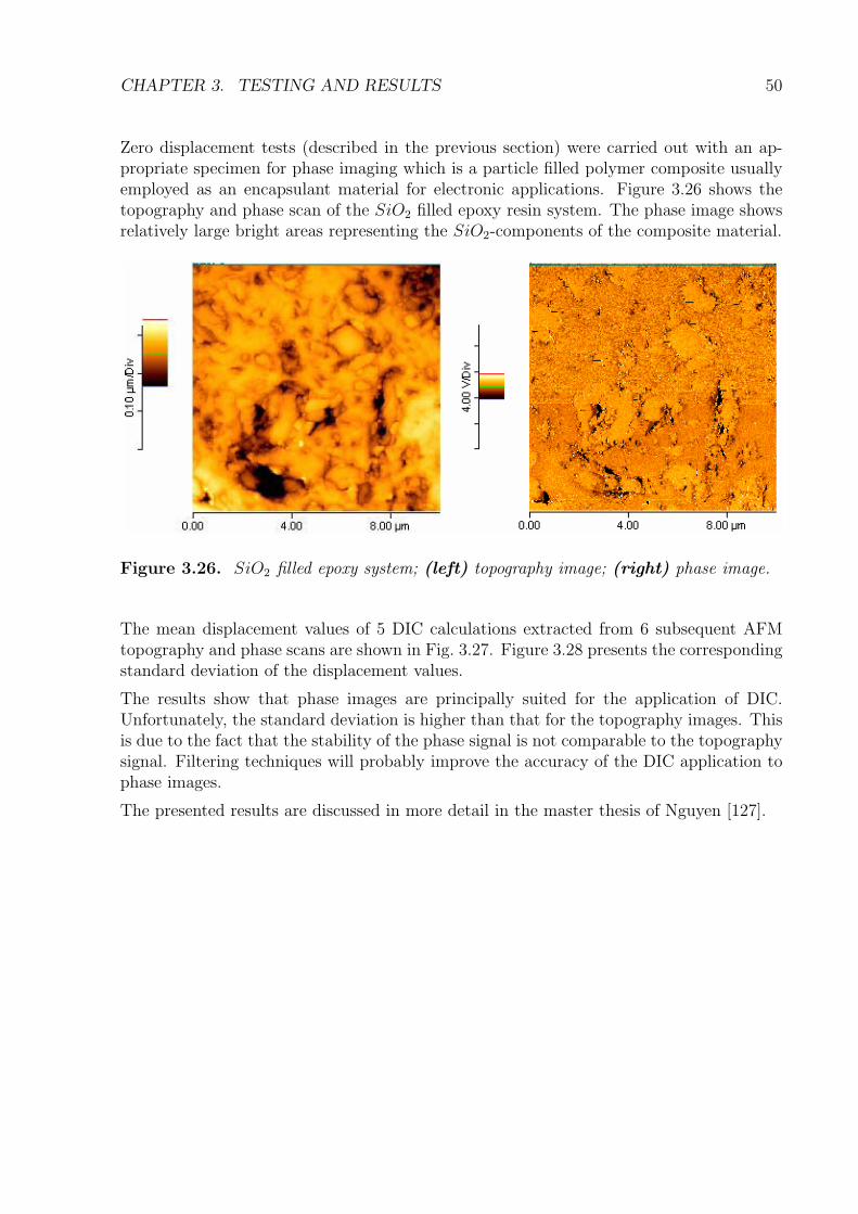
CHAPTER 3. TESTING AND RESULTS 50
Zero displacement tests (described in the previous section) were carried out with an ap-propriate specimen for phase imaging which is a particle filled polymer composite usuallyemployed as an encapsulant material for electronic applications. Figure 3.26 shows thetopography and phase scan of the SiO2 filled epoxy resin system. The phase image showsrelatively large bright areas representing the SiO2-components of the composite material.
Figure 3.26. SiO2 filled epoxy system; (left) topography image; (right) phase image.
The mean displacement values of 5 DIC calculations extracted from 6 subsequent AFMtopography and phase scans are shown in Fig. 3.27. Figure 3.28 presents the correspondingstandard deviation of the displacement values.
The results show that phase images are principally suited for the application of DIC.Unfortunately, the standard deviation is higher than that for the topography images. Thisis due to the fact that the stability of the phase signal is not comparable to the topographysignal. Filtering techniques will probably improve the accuracy of the DIC application tophase images.
The presented results are discussed in more detail in the master thesis of Nguyen [127].

CHAPTER 3. TESTING AND RESULTS 51
0
0.02
0.04
0.06
0.08
0.1
0.12
1 2 3 4 5
u topo u phase u topo u phase
Measurement No.
Mean D
ispla
cem
ent [µ
m]
x x y y
Figure 3.27. Mean displacement values of DIC results extracted from topography andphase images [127].
0.000
0.002
0.004
0.006
0.008
0.010
0.012
0.014
0.016
0.018
1 2 3 4 5
u u phase u topo u phase
Measurement No.
Sta
ndard
Devia
tion [µ
m]
topox x y y
Figure 3.28. Standard deviation values of DIC results extracted from topography andphase images [127].

CHAPTER 3. TESTING AND RESULTS 52
3.4.4 Results of In-Situ AFM Measurements
The analysis of crack tip behavior by means of AFM based deformation measurementtechnique should give new insights into the micro- and nanostructural behavior of polymericmaterials during loading. For the investigated polymers the question whether continuummechanics prevail or at what scale other concepts have to be taken into account should beanswered with deformation measurements of varying AFM scan sizes. With the strategyof zooming into the vicinity of the crack tip micro- or nanostructural discontinuities of thematerials should be detectable.
Therefore, in-situ AFM measurements were carried out at CT-specimens with a specimenwidth W = 20 mm in correlation to the geometry given by Fig. 2.10. The loading wasapplied in three load steps using the tension/compression testing module (Fig. 3.16). Anoverview of the load steps and the applied AFM scan sizes are given in Table 3.3.
Table 3.3. Load steps and scansizes of in-situ AFM crack analysis.
Load steps F1 → F2 [N] Scan size [µm]
1 8.3 → 16.4 15 × 152 16.4 → 20.7 4.6 × 4.63 20.7 → 24.4 2.5 × 2.5
0 20 40 60 80 1000
5
10
15
20
25
30
Load
F [N
]
Displacement δ [µm]
8.3
16.4
20.7
24.4AFM scans at 4 load states
Figure 3.29. Loading of cynate ester CT-specimen; load states are marked.
During the AFM scans the drive of the motor was stopped while the load monitoring wascarried on. Figure 3.29 shows the complete loading scheme.

CHAPTER 3. TESTING AND RESULTS 53
Note that ”running-in” at the beginning of the load-displacement curve is due to inden-tation of the loading pins. The graph shows that stopping of the loading process is not aproblem for this kind of polymer material. The viscoelasticity has only a small effect onthe loading curve so that the stress relaxation is negligible to a certain extent. Neverthe-less, the effect of viscoelastic material behavior on the deformation field at the crack tip isanalyzed by finite element analysis and a discussion of the results is given in Sect. 4.4.
In the following the crack opening displacement fields (displacement in y-direction) of thementioned load steps are shown. Digital image correlation analysis of the AFM topographyimages of load steps 1, 2 and 3 result in the y-displacement fields which are illustrated inFigs. 3.30-3.32. For the load step 3 the DIC analysis was also applied to the error signalimages (compare to Fig. 3.33).
The results show the principal capability of the method for crack tip field analysis. Fromthe comparison of Figs. 3.30, 3.31 and 3.32, the down scaling capability is obviously proven.In addition to the presentation of the displacement results obtained from the various loadstates the crack opening fields are also directly compared to each other. With the assump-tion of linear elastic behavior the fields of the 2nd and 3rd load state are scaled (with afactor related to the applied loads) where the results originating from the 15 µm scansserve as the reference load state. Figure 3.34 shows the displacement fields from the 1stload state together with the adjusted field from the 2nd load state and Fig. 3.35 showsan analogous presentation of the 2nd and the 3rd field. It is obvious that a completequantitative agreement of the displacement fields is not given. Possible reasons may befound in an inaccurate loading regime which still has the rotation around the x-axis as arestricted degree of freedom so that a accurate mode I crack opening cannot be achieved.Another source for the inconsistencies may be the existence of material inhomogeneities.In addition the DIC analysis using topographic AFM images of the same object but withdifferent scan sizes are not fully comparable. Depending on the surface topography smallimages do often not render the required contrast for a high accuracy image correlation.
The comparison of the results of Fig. 3.32 and 3.33 shows that error images are also suitedfor the application of DIC. The extracted crack opening displacement field as shown inFig. 3.33 is similar to field calculated from topographical images (Fig. 3.32). Error imagesof small size areas of surfaces with low roughness value reveal better contrasts than theircorresponding topography images. This leads to more accurate results of the appliedcorrelation algorithms. Nevertheless it has to be noted that it is difficult to give an a-prioristatement on wether the error or the topography images are better suited for the DICanalysis. The decision have to be taken from case to case what type of analysis results aremore trustworthy. For the complete understanding of the accuracy of SPM image basedDIC technique, more detailed research will have to be carried out. However, rapid changesin SPM equipment will overcome several findings on this research field.
The presented results and the discussion leads to the following closing remarks for SPMbased DIC analysis:
• A minimum variation of the gray values (in the case of topographic AFM images:surface roughness) across the image area is required for a high precision DIC anal-ysis. Note that small kernel sizes can be more accurate for the detection of plastic

CHAPTER 3. TESTING AND RESULTS 54
deformations than larger kernel sizes due to the fact that with increasing kernel sizesthe integration effect will also increase. This means that plastic deformation effectscan be smeared out with kernel sizes which are chosen too large.
• DIC results based on different scan sizes are not fully comparable. Data variation(in the case of topographic AFM images: surface roughness) should be similar.
• A complete description of the accuracy of a SPM image based DIC analysis will bea cumbersome procedure. The following parameters have to be taken into account:Data variation of the relevant imaging technique (topography, error, phase, etc.), tipshape, tip to surface interaction (contact or noncontact mode, height), reaction (gain)of feedback loop in z-direction, repositioning accuracy in x, y-direction (linearizationproblem of piezo)
• New generations of SPMs will overcome several of the described stability and accuracyproblems.
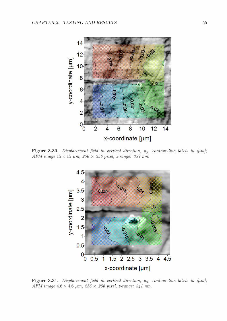
CHAPTER 3. TESTING AND RESULTS 55
Figure 3.30. Displacement field in vertical direction, uy, contour-line labels in [µm];AFM image 15 × 15 µm, 256 × 256 pixel, z-range: 357 nm.
Figure 3.31. Displacement field in vertical direction, uy, contour-line labels in [µm];AFM image 4.6 × 4.6 µm, 256 × 256 pixel, z-range: 344 nm.
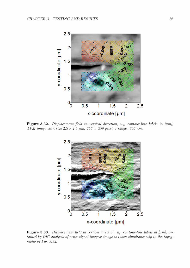
CHAPTER 3. TESTING AND RESULTS 56
Figure 3.32. Displacement field in vertical direction, uy, contour-line labels in [µm];AFM image scan size 2.5 × 2.5 µm, 256 × 256 pixel, z-range: 306 nm.
Figure 3.33. Displacement field in vertical direction, uy, contour-line labels in [µm]; ob-tained by DIC analysis of error signal images; image is taken simultaneously to the topog-raphy of Fig. 3.32.

CHAPTER 3. TESTING AND RESULTS 57
Figure 3.34. Displacement field, uy, contour-line labels in [µm], for 15 × 15 µm and4.641 × 4.641 µm scan.
Figure 3.35. Displacement field, uy, contour-line labels in [µm], for 4.641 × 4.641 µmand 2.5 × 2.5 µm scan.

CHAPTER 3. TESTING AND RESULTS 58
3.5 Fractography by SEM and SPM methods
In addition to the AFM topography analysis of the fracture surface SEM images weretaken. SEM images give a better overview of the fracture processes occurred during crackpropagation. Zones of slow or rapid fracture and crack arrest lines can be easily identified.
All SEM images are taken with a tilting angle of 20 ◦ to the fracture surface so that onlythe dimensions in horizontal direction are in correlation with the included scales. Figure3.36 shows the fracture surface of a cyanate ester CT-specimen. In the image on the lefthand side a region of cascade-like markings are observed. A detail of this region is givenin Fig. 3.36 (right). This kind of fracture topography is the result of a crack propagationwhich is driven by a mixed mode loading due to a crack front deflection similar to Fig.3.12.
razor blade induced pre-crackrazor blade induced pre-crack
markings due tomarkings due to
deflected crack frontdeflected crack frontsteady-state steady-state
crack growthcrack growth
Figure 3.36. Fracture surface of CE CT-specimen; (left) overview of the crack initiationzone, steady-state crack propagation is achieved at the bottom of the image; (right) detailof markings caused by a deflection of the crack front in y-direction.
Figure 3.37 shows an overview (left) and a detail (right) of the fracture surface formed bysteady-state fracture propagation. It has to be noted that the crack surface is very smooth.Topographical fracture features at the micro scale cannot be observed. In contrast to thesmooth crack propagation of the neat CE resin the fracture surface of the rubber modifiedCE shows topographic features which are stretched in crack growth direction (compareFigs. 3.37 and 3.39). Although the crack propagation of the rubber modified CE occursin a stick-slip type, there are no significant topographic differences between the surfaceformed during steady state crack propagation and that during crack jump.
SEM images of the crack tip opening taken just before the crack propagation clearly showsthe difference between the neat and the rubber modified CE (Fig. 3.40). The response of

CHAPTER 3. TESTING AND RESULTS 59
Figure 3.37. Region of steady-state crack growth at CE fracture surface, note that thehorizontal and vertical lines are not fracture features, but caused by cracks in the carbonsputtering layer; (left) overview; (right) detail.
the blended thermoset system to the critical loading is accompanied by the effect of cracktip blunting. Traces of the blunting are also visible after a small crack propagation (Fig.3.41). The microcracks at the crack faces may originate from residual stresses induced bymechanical polishing of the surface. They cannot be identified as crazes.
In addition to the SEM observations AFM tapping mode phase image scans were carriedout at the crack surface of a neat and rubber modified CE specimen. Unfortunately,different phases could not be identified in a reproducible and reliable way so that theresults are not shown in this work. The reason might be that the dimensions of the phasesare too small (in the nm range) for a reliable SPM-based detection and/or the variation inmechanical properties of the two phases is too low to obtain a significant shift of the phasesignal. Other researchers [16] identified different phases (in the micrometer range) by phasedetection microscopy at fracture surfaces of similar material systems. Therefore, furtherresearch on fractography approach by SPM techniques has to be done. A variety of differentSPM analysis modes such as AFAM or UFM are available from different manufacturersand research groups. Depending on the material class, the one or the other method willbe promising. Nowadays, a universal SPM method for the determination of qualitativeand quantitative mechanical properties is not established. Another promising approach forthe detection of different phases of the discussed rubber modified CE is the application oftransmission electron microscopy (TEM).

CHAPTER 3. TESTING AND RESULTS 60
detaildetail
Figure 3.38. Fracture surface of rubber modified cyanate ester resin; (left) overview,several crack arrest lines from razor blade pre-crack are visible in the upper part of theimage, the flake like features on the right hand side of the image are caused by cracks inthe carbon sputtering layer; (right) detail, starting line of rapid fracture propagation.
Figure 3.39. Fracture surface of rubber modified cyanate ester resin; crack arrest line, asmall region of steady state crack growth and starting line of rapid crack growth are shown;(left) overview; (right) detail.

CHAPTER 3. TESTING AND RESULTS 61
Figure 3.40. Crack tip opening before fracture of (left) neat cyanate ester resin and(right) rubber modified cyanate ester resin.
Figure 3.41. Crack tip after a small crack propagation of rubber modified cyanate esterresin; traces of crack tip blunting are visible; the microcracks at the crack faces are possiblycaused by stresses induced by mechanical polishing of the surface.

Chapter 4
Discussion - Comparison ofExperiment and Simulation
The verification of numerical reliability estimation of a microelectronic system by theapplication of experimental techniques is a fundamental task. Due to the fact that in manycases experimentally derived material properties are not available for structural componentshaving one or more dimension in the range of nanometers the inversion of this approach is ofmajor interest for nanotechnological devices of the future. If material properties of a systemcomponent cannot be validated by an appropriate measurement technique the DIC-baseddisplacement analysis enables a better understanding of the thermomechanical materialproperties. For example a new technological process for the fabrication of thin films maychange the material behavior dramatically (e.g. isotropic to anisotropic, linear elastic toplastic, etc.). In such cases, a comparison of FE-results with strain field measurements andrecursive material model variation of the FE-model leads to improvements of the reliabilitysimulation. The ongoing development of fully parameterized FE-modeling techniques willfacilitate this approach [128].
Due to the fact that the importance of the combination of simulation and experiments willincrease for future developments of microelectronic systems, MEMS and NEMS a powerfulreliability assessment tool is necessary. Starting with an analytical crack evaluation concept(Sect. 4.1) the main focus of this chapter is laid on the definition and implementation of ahybrid analysis tool combining SPM based experimental displacement measurements andfinite element concepts (Sect. 4.6). The basis of this strategy is an adaptation conceptwhich will be discussed in detail.
Throughout this chapter, the developed concepts are consistently applied to the measure-ments carried out at the CT-specimen discussed in Sect. 3.4.4.
4.1 Crack Opening Displacement Analysis
The classical stress intensity factor K is conventionally determined by means of macroscopicfracture tests at standardized fracture specimens such as the CT-specimen. A straight-forward approach for crack evaluation by means of AFM images is the technique of crackopening displacement (COD) determination.
62

CHAPTER 4. DISCUSSION - COMP. OF EXPERIMENT AND SIMULATION 63
In order to determine the mode I stress intensity factor KI crack opening displacementsuu
y and uly are measured along both the upper and lower crack boundaries.
uyl (x)
x
yr
uyu(x)
uyr(x)
crack
Figure 4.1. Crack opening displacement according to LEFM for infinite bulk materialand mode I crack opening.
If determined by linear elastic fracture mechanics they must equal to
uu,ly = ±KI
2µ
√x
2π(κ + 1)
uuy = ul
y = 0
x ≤ 0 (4.1)
x > 0 (4.2)
where µ is the shear modulus and κ is a function of Poisson’s ratio, ν (compare to Eqns.2.7 and 2.8). Taking the square of the difference of upper and lower displacements, weobtain a linear function of the x-coordinate or 0, depending on the position relative to thecrack tip:
(uu
y − uly
2
)2
= Cx
= 0
x ≤ 0 (4.3)
x > 0 (4.4)
The expression of Eqn. 4.3 does not change if specimen rotation due to inaccurate loadingis included into the considerations. In this case, equal rotational terms on both sides ofthe crack boundary are subtracted from each other. For the equation above, the crack tipis set at location x = 0. The crack tip location on the real specimen can be found at theinterception of a linear fit of the curve Cx with the x-axis. The slope C allows to estimatethe stress intensity factor KI , which is a measure of the crack tip load. It is given by:
KI =E
1 + ν
1
κ + 1
√2πC (4.5)
The discussed analysis is applied to the measurements presented in Sect. 3.4.4. The resultsfor the 15 × 15µm scans are shown in Fig. 4.2.
The determined value for KI with the application of Eqn. 4.5 and the assumption ofthe plane strain solution equals to 0.056 MPam1/2. The value calculated from the appliedloads is 0.085 MPam1/2. The comparison shows that the value calculated from the specimenloading is 1.5 times higher than the value extracted from the crack opening field.

CHAPTER 4. DISCUSSION - COMP. OF EXPERIMENT AND SIMULATION 64
uyl
uyu
2 4 6 8 10 120.000
0.001
0.002
0.003
0.004
0.005
0.006
����
�����
� �������
������������� ��
� � � �����������
� � � ������� ���
Figure 4.2. (left) AFM image of crack tip area (size: 15 × 15 µm) with overlaid dis-placement results in y-direction, uy; lines for the upper and lower crack face are also shown(right) evaluation of slope C for the calculation of the stress intensity factor KI .
Possible reasons or error sources for the deviation are:
• the value of the measured Young’s modulus is too low for this CT specimen so thatthe field determined KI-value is also underestimated,
• the crack is not fully loaded at the surface of the specimen, due to the fact that (inthis case) the crack front is a relatively straight line normal to the specimen surface,
• the evaluation of the slope Cx is based on displacements of the upper and lower crackface which are extracted from DIC results. The distance of the corresponding lines(compare to Fig. 4.2) to the crack face is not zero so that the calculated slope andthe stress intensity factor is lower than the actual value.
• the plane stress or strain crack field solution is not accurate or is not completelypredominating at the surface of the specimen.
Concluding the results discussed in this section, a detailed analysis of the crack tip behaviorby FE simulation is necessary.
4.2 Finite Element Model
In order to compare SPM measurements with numerical solutions based on finite elementmethod the problem of a wide range of element sizes (from the mm- to nm-scale) has tobe taken into account. For modeling the surrounding of the crack tip a very fine meshis necessary compared to the global size of the CT-specimen. Small element edges in thex-y-plane in combination with a coarse mesh in the z-direction will cause element shape

CHAPTER 4. DISCUSSION - COMP. OF EXPERIMENT AND SIMULATION 65
problems. For accurate numerical results an element edge size ratio not lower than 1/10has to be achieved. The problem can be solved by the submodeling technique which wasapplied to several numerical calculations presented in this chapter. An illustration of thecreated FE model is given in Fig. 4.3.
Submodel 1
60 µm
Submodel 2
500 µm
Figure 4.3. Principle of submodeling technique for accurate modeling of the crack tip, asapplied to PATRAN/ABAQUS FE-models.
The CT-specimen is modelled in a global model with the relevant boundary conditions(force or displacement) applied to the loading pins and a solution is computed with theFE-solver (ABAQUS, ANSYS). A local model is built up in the surrounding of the cracktip using the same coordinate system as the global model. Afterwards, the cut boundarywith the global model is determined and the nodal displacement solution of the globalmodel (at the cut boundary) is transferred to the local model arranging the boundarycondition for the second solution process. In general, the FE-software interpolates thedisplacement values from the coarse global mesh to the finer local mesh. This is the keyfor the implementation of a submodeling technique. A nesting of submodels can also beperformed.
The actual FE approach of the CT-specimen is built up by two step submodeling. Thefirst local mesh models the crack front boundary over the complete specimen thickness B.In a second submodel, only a small volume at the surface is redefined with a finer mesh(Fig. 4.3) enabling the adaptation of the FE-mesh to the in-situ loading experiments. Adetailed description of the mesh interface for a quantified comparison of numerical andexperimental approaches is given in Sect. 4.6.2.
In the following sections, several numerical results are presented basing on the discussedor slightly modified model. The applied modifications are summarized as follows:
• Variation of crack front curvature from a straight to a curved shape.

CHAPTER 4. DISCUSSION - COMP. OF EXPERIMENT AND SIMULATION 66
• Modification of material model from linear-elastic to viscoelastic.
• Modification of material model from linear-elastic to plastic.
The intention behind these modifications and the corresponding results are presentedthroughout Sect. 4.3 - 4.5.
4.3 Crack Front Curvature
The crack front of a CT-specimen with finite thickness tends to form a curvature such thatthe crack in the middle of the specimen is running ahead of the crack front at the edgeof the specimen, Fig. 4.4 (left). This is the result of the three dimensional character ofthe crack tip stress field. At the edge of the specimen the material can expand in the z-direction whereas in the middle the expansion in z-direction is restricted to a large extent.This phenomenon is often [82] described as prevailing state of plane strain (in the middleof the specimen) and plane stress (at the surface of the specimen).
crack arrest line
razor blade induced crack
steady state crack growth
rapid crack growth
Figure 4.4. Curved crack front at CT-specimen (left) For a (rubber modified) thermosetmaterial, crack initiation and crack arrest lines after rapid crack propagation are observed(stick-slip); (right) FE-model of CT-specimen with curved crack front.
The effect of the crack front curvature is analyzed by a modified FE-model as illustratedin Fig. 4.4 (right). The global boundary conditions of the FE model are not modified.The curvature is modelled by a polynomial function of order 2, with the x-direction of thecrack tip at the specimen surface for straight and curved crack front being identical. In themiddle of the specimen the crack front is running 0.5 mm ahead compared to the specimensurface. This value was typical for the modified cyanate ester resins as it is illustrated inFig. 4.4 (left).

CHAPTER 4. DISCUSSION - COMP. OF EXPERIMENT AND SIMULATION 67
In an FE-analysis the effect of the formation of the crack front curvature can be analyzedby means of energy based integral calculations such as the J-integral (Eqn. 2.17). Figure4.5 shows the value for the J-integral over the thickness coordinate z (compare to Fig. 2.7)for a straight and a curved crack front.
0 1 2 30.0
0.1
0.2
0.3
straight crack front(before crack propagation)
curved crack front (after crack propagation)
J-In
tegr
al [N
/mm
]
z - Coordinate at Crack Front [mm]
Figure 4.5. J-integral vs. z-direction for a straight and a curved crack front.
For both numerical solutions the J-integral varies with the location at the z-direction ofthe specimen. The largest value is observed in the middle of the specimen (z = 0) fromwhere it is steadily decreasing towards the specimen surface. This means that the crackgrowth will be initiated in the middle of the specimen followed by the specimen edges.With a curved crack front the variation of the J-integral towards the edge of the specimenis reduced (Fig. 4.5). The crack driving energy is becoming balanced over the crack frontto a large extent. However, it has to be noted that the crack front as it is modeled in thisanalysis (polynomial function of order 2) is not identical with the actual experimental crackfront. This approach is only valid to show tendencies of crack front curvature formation.More accurate modeling of the crack front curvature may lead to better balance of theJ-integral over the z-direction.
Besides the formation of the crack front curvature, the effect of a present curved crack fronton the experimental approaches of this work has to be analyzed. Regarding the appliedmeasurement techniques of OCT and DIC two effects have to be taken into account:
• Effect of curved crack front on the measured R-curve at the beginning of the fractureprocess. – The straight crack front induced by tapping of a razor blade is the result ofa rapid crack propagation. Therefore, the crack front is not equivalent to the curvedcrack front during a steady state or stick-slip type of crack propagation.
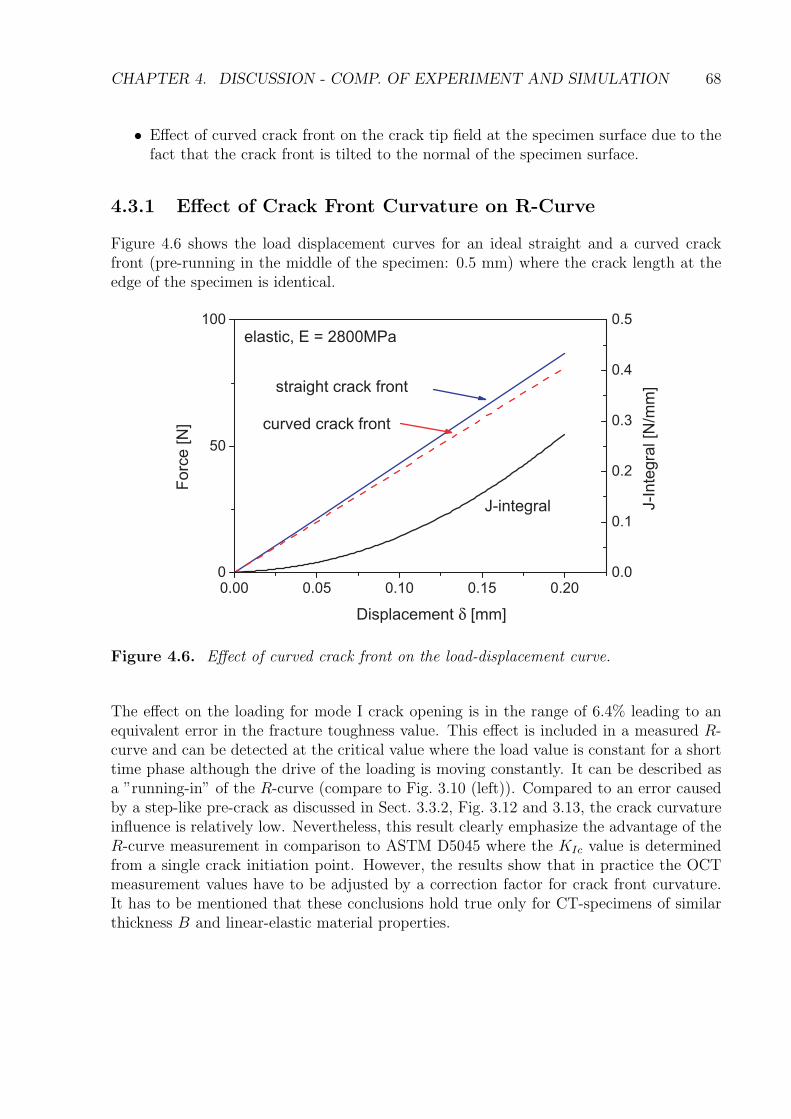
CHAPTER 4. DISCUSSION - COMP. OF EXPERIMENT AND SIMULATION 68
• Effect of curved crack front on the crack tip field at the specimen surface due to thefact that the crack front is tilted to the normal of the specimen surface.
4.3.1 Effect of Crack Front Curvature on R-Curve
Figure 4.6 shows the load displacement curves for an ideal straight and a curved crackfront (pre-running in the middle of the specimen: 0.5 mm) where the crack length at theedge of the specimen is identical.
0.00 0.05 0.10 0.15 0.200
50
100
elastic, E = 2800MPa
J-integral J-I
nte
gra
l [N
/mm
]
Forc
e [N
]
Displacement δ [mm]
0.0
0.1
0.2
0.3
0.4
0.5
curved crack front
straight crack front
Figure 4.6. Effect of curved crack front on the load-displacement curve.
The effect on the loading for mode I crack opening is in the range of 6.4% leading to anequivalent error in the fracture toughness value. This effect is included in a measured R-curve and can be detected at the critical value where the load value is constant for a shorttime phase although the drive of the loading is moving constantly. It can be described asa ”running-in” of the R-curve (compare to Fig. 3.10 (left)). Compared to an error causedby a step-like pre-crack as discussed in Sect. 3.3.2, Fig. 3.12 and 3.13, the crack curvatureinfluence is relatively low. Nevertheless, this result clearly emphasize the advantage of theR-curve measurement in comparison to ASTM D5045 where the KIc value is determinedfrom a single crack initiation point. However, the results show that in practice the OCTmeasurement values have to be adjusted by a correction factor for crack front curvature.It has to be mentioned that these conclusions hold true only for CT-specimens of similarthickness B and linear-elastic material properties.

CHAPTER 4. DISCUSSION - COMP. OF EXPERIMENT AND SIMULATION 69
4.3.2 Effect of Crack Front Curvature on Crack Tip Field
For the measurement of deformation fields at specimen surfaces the curvature of the cracktip cannot be neglected. Goken and Vehoff showed by FEA that displacement fields canbe significantly influenced by the angle between the crack front and the specimen surface[21, 22]. Figure 4.7 shows the results of FE-analysis calculated with a straight and acurved crack front. In the middle of the specimen the crack front is running 0.5 mm aheadcompared to the specimen surface leading to an angle of 19.3 ◦ between the crack front andthe normal of the surface area.
Figure 4.7. Crack tip displacement field in y-direction, uy in [mm]; (left) straight crackfront; (right) curved crack front.
The comparison of the fields show that the displacement values at the crack field are1.7 times higher for the FE calculation based on a curved crack front. This result is incorrelation with the J-integral across the specimen thickness, (compare to Fig. 4.5). Theloading of the crack front at the surface is lower for a straight crack than for a curvedcrack. This result clearly emphasizes that an accurate crack evaluation by experimentalmethods has to be verified by finite element simulations with models representing theactual geometry of the specimen with a high accuracy.
4.4 Influence of Viscoelasticity on Crack Tip Field
The question of the effect of a viscoelastic in comparison to an elastic model is answeredby simulation. FE calculations were carried out with the model of Fig. 4.2 and viscoelasticmaterial model as defined in Sect. 3.2.5.
For the chosen materials the effect of viscoelasticity on the loading and the crack tip fieldis negligible. Due to the fact that the results are nearly the same (effect below 0.1%) theyare not presented in this work.

CHAPTER 4. DISCUSSION - COMP. OF EXPERIMENT AND SIMULATION 70
4.5 Influence of Plasticity on Crack Tip Field
At the crack front of polymer materials, several failure modes such as blunting effects,crazes, microcracks, microvoids may be observed. Although these effects were not observedin the performed SPM measurements an estimation of the size of the plastic zone is carriedout. Therefore, a numerical simulation is performed with an FE-model analogous to Fig.4.3 where the material model is defined including perfect plasticity with a flow stress of50 N/mm2. The corresponding stress-strain curve of the material model is defined asillustrated in Fig. 4.8 (left).
0.00 0.01 0.02 0.03 0.040
25
50
75
elastic, E = 2800MPa
Str
ess
[N/m
m2]
Strain
perfect plasticity
0 1 2 30.0
0.1
0.2
0.3
JG-integral for plastic case,
perfect plasticity: 50 N/mm2
J-integral for elastic caseJ G-
& J
-Int
egra
l [N
/mm
]
z - Coordinate at Crack Front [mm]
Figure 4.8. Material model for perfect plasticity. Effect of plasticity on J-integral alongthe crack front.
The effect of plasticity on the crack front behavior is analyzed by a generalized J-integralapproach developed by Ghavifekr [91] (compare to Eqn. 2.18). The results are shown inFig. 4.8 (right).
Similar to the effect of crack front curvature formation also plasticity causes the ”flattening”of the J-integral over the specimen thickness. This is the result of the ability to react withlarge inelastic strains. However, in this work prevailing of a large plasticity zone was notverified by the experimental displacement field measurements.
Figure 4.9 shows the von Mises stresses around the crack tip at the specimen surfaceextracted from linear-elastic simulation. The results are presented for a loading of F = 86 Nwhich is already above the fracture toughness of the actual cyanate ester resin. At thesurface of the specimen the plastic simulation did not show a significant influence on thestress field so that the numerical results are not shown here. However this underlines theexperimental observation that a plastic zone was not detected by the application of DICto the crack tip images obtained by AFM.
A comparison of von Mises stresses of the CT-specimen based on linear-elastic and plasticmaterial model are given in Fig. 4.10 and 4.11. As the coordinate systems indicate the Figs.illustrate the stress solution of the center of the specimen where the effect of plasticity isobviously more evident. With the assumption of perfect plasticity the size of the plasticzone at the crack tip would be in the range of 1 µm (compare to Fig. 4.11). Such a large

CHAPTER 4. DISCUSSION - COMP. OF EXPERIMENT AND SIMULATION 71
Figure. 4.9. Von Mises stress at crack tip at specimen surface for linear-elastic simula-tion.
plastic zone was not detected in the SPM experiments. This result also correlates to thefractographic analysis (compare to Sect. 3.5) of the fracture surface revealing no indicationfor the formation of a plastic zone in the µm range.
The conclusion of the experimental approach and the verification with FE-results clearlyemphasize the predominating linear-elastic material behavior of the investigated cyanateester resin.

CHAPTER 4. DISCUSSION - COMP. OF EXPERIMENT AND SIMULATION 72
Figure 4.10. Von Mises stress at crack tip in the middle of the specimen for linear-elasticsimulation.
Figure 4.11. Von Mises stress at crack tip in the middle of the specimen for plasticsimulation; a plastic zone of ≈ 1 µm.

CHAPTER 4. DISCUSSION - COMP. OF EXPERIMENT AND SIMULATION 73
4.6 Adaptation Strategies between Simulation
and Experiment
The presented FE-results of the previous sections clearly underline the difficulties involvedin the experimental crack tip evaluation at the micro and nanoscale. Moreover, micro- andnanocracks in real electronic systems, MEMS or NEMS are nested in a variety of materialswith different material properties. In such cases, the experimental approach on its ownis not suited for the determination of critical stress/strain states or system reliability. Apossible solution is the strategy of using a hybrid analysis tool combining SPM-basedexperimental displacement measurements and finite element concepts. In this work suchan approach is implemented by a definition of an adaptation concept which is presented inSect. 4.6.1. The basis for the concept is the mesh adaptor enabling the reduction of 3D-FEmesh data to 2D-DIC software node coordinate data (Sect. 4.6.2). Furthermore, a commonplatform for FEA and DIC results is defined (Sect. 4.6.3) and a verification algorithm forsimulation/experimental results is developed (Sect. 4.6.4).
The developed strategy is applied to the measurements of Sect. 3.4.4 in combination withFE-results basing on the models described in Sect. 4.2.
4.6.1 Adapted Finite Element Concept
The objective of an adapted finite element concept is the creation of a tool which allows theverification of in-situ loading experiments and finite element results using a combination offinite element simulation and DIC-based displacement fields. FEA on its own is not suffi-cient to describe complex material and device behavior for future micro and nanomaterialtesting. Unknown material constitutive laws and complex interrelation between testingequipment and specimen make it unreliable to evaluate reliability exclusively by FEA oranalytical approaches. Consequently validation of mechanical test modeling by suitableexperiments is inevitable.
Comparison between measured and simulated deformation fields is the way to achievetrustworthy testing results. Unfortunately, in many cases simple determination of materialproperties by DIC measurements is impossible since there is the general access restrictionof DIC measurements to surface and in-plane deformation. 3D and internal deformationdata is indispensable for many testing purposes, e.g. for the determination of parametersfor advanced fracture mechanics criteria (J-, C�-, T -integral, etc.). Moreover, in somecases stress/strain data on three dimensional objects is needed, which cannot be obtainedfrom in-plane surface measurements. This information can be provided adapting FEA toDIC measurement. Due to the fact that both methods are implemented in completelydifferent and therefore incompatible software packages an adaptation concept from FEAto DIC was developed. A flow chart of the concept is shown in Fig. 4.12.
Basically, the concept allows to match simulation and measurement results in order toprovide material characterization on a best-fit strategy. At the end, material propertiessuch as Young’s modulus or fracture mechanical properties are determined combining FEAand DIC results. FE meshes from either PATRAN/ABAQUS or ANSYS are utilized for

CHAPTER 4. DISCUSSION - COMP. OF EXPERIMENT AND SIMULATION 74
C
rack T
est S
pe
cim
en
F
E M
od
elin
g(P
AT
RA
N/A
BA
QU
S, A
NS
YS
)
geo
metr
ical
m
ode
l
co
nstitu
tive
be
havio
r
lo
ad
co
nd
itio
ns
F
E A
na
lysis
(F
EA
)
AB
AQ
US
, A
NS
YS
DIC
me
asu
rem
ent
AD
AS
IM s
oft
wa
re
R
igid
bo
dy
dis
pla
ce
me
nt
an
d r
ota
tion
a
dju
stm
en
t
Be
st
fit
eva
lua
tio
n
by
co
mp
ari
so
n b
etw
ee
n F
EA
and
me
asure
me
nt re
su
lts
dis
pla
ce
me
nt
fie
lds:
se
rie
s f
or
diffe
ren
t lo
ad
sa
nd
/or
ma
teria
l p
rop
.
3
D t
o 2
D p
roje
ctio
no
f F
EA
mesh
an
d r
esu
lts
R
es2
DIC
so
ftw
are
or
A
NS
YS
-AP
DL m
acro
De
term
ina
tion
of fr
actu
re p
ara
me
ters
for
se
lecte
d f
ractu
re c
rite
rion
an
d b
est
exp
erim
en
tal fit
co
nd
itio
ns
2D
measure
ment m
esh
identically
with F
EA
mesh
poin
ts a
nd/o
r a
rea
s o
f defined r
igid
body
dis
pla
cem
ent and r
ota
tion
avera
ge d
ispla
cem
ent
and
rota
tion o
ver
a c
ert
ain
obje
ct are
a
best fit m
ate
rial data
and/o
rlo
adin
g c
onditio
ns
�
�
�
��
�
Fig
ure
4.1
2.
Ada
ptat
ion
conce
pt.

CHAPTER 4. DISCUSSION - COMP. OF EXPERIMENT AND SIMULATION 75
simulation as well as for DIC displacement field determination from load state images (see➀ in Fig. 4.12). Therefore, a transformation interface of FE mesh nodes to respectivemeasurement mesh nodes have to be developed. 3D-to-2D mesh transformation, data(node) reduction and allocation of object and model coordinates are the major problemsto be solved.
Although determined in the same mesh nodes, simulation and measurements results cannotbe compared directly. DIC deformation fields are superposed by rigid body displacementsand rotations originating from, e.g. , testing machine drifts, or FE boundary conditionswhich are not equivalent to the actual experimental loading. Therefore, original DIC resultshave to be derotated and a translation correction has to be applied before comparingthem with FEA fields (see ➁ in Fig. 4.12). Within the concept, a set of finite elementdisplacement fields is compared with a set of derotated and displaced measurement fields(➂ in Fig. 4.12). Different simulated fields are provided varying specimen load conditionsor material properties. The best fit between simulation and measurement field reveals theoptimum input data (modeling) for simulation with regard to the specimen load conditionsunder consideration. Utilizing these best fit conditions proven by experiment, additionalor more advanced material properties can be produced demanding more information thanDIC measurements can provide (➃ in Fig. 4.12).
4.6.2 Mesh Transfer from FEA to Experiment
Transfer of finite element nodes to the measured experimental area is a straightforwardapproach for data comparison. This technique allows to determine the experimental dis-placements at the position of the FE nodes so that a direct validation of the results can beperformed. Figure 4.13 illustrates the concept of the mesh adaption from 3-dimensionalFE model to 2-dimensional region-of-interest (ROI) of the experimental approach.
The digital image correlation technique determines displacements at specific grid nodeswhich are similar to the nodes of the finite element mesh. In addition to meshing by meansof an internal mesh generator the DIC software allows to import user defined meshes.During this mesh-import procedure the user has to specify x, y-scaling factors for thetransformation of [mm]-based node location (from FE-model data) to [pixel]-coordinates(of measurement images).
In the presented case, the mesh adaptation is carried out between the FE-code ANSYS andthe DIC software ADASIM using ANSYS parametric design language (APDL). The appli-cation of APDL introduces a functionality allowing a fast postprocessing and streamlinesthe data extraction form the FE-model to the DIC software. The implemented interfacemacro is structured as follows:
1. defining of an region-of-interest (ROI) area by user defined (mouse) picking of 4 edgenodes,
2. definition of result coordinate system aligned with the coordinate system of the user-defined ROI area,

CHAPTER 4. DISCUSSION - COMP. OF EXPERIMENT AND SIMULATION 76
3D FE model extracted 2D mesh 2D mesh adapted to DIC software
1
4 3
2
Figure 4.13. Concept of mesh adaption from FEA- to DIC-software.
3. printout of the node coordinates and element definitions of the ROI area; the nodeindices have to be re-organized from ANSYS notation to the notation implementedin ADASIM; details on node notations can be found in the ANSYS and ADASIMuser manuals [129,130]
4. printout of the results (node displacements).
The interface macro produces mesh input files according to the interface definition ofADASIM. A detailed description of the APDL code is not necessary. The programmingcan be actualized relatively straightforward by implementation of the concept describedabove.
Figure 4.13 illustrates mesh adaptation for the rather simple case of the CT-specimen whichis the test specimen within this work. Nevertheless, the basic idea of this mesh adaption canalso be applied to more complex structures of microelectronic components. In this case theregion of interest can be e.g. mechanically weak parts of a micro- or nanostructured solderbump or ultrathin passive or active layers. In microelectronic applications, usually a largenumber of different materials is combined on a small volume. This results in a varietyof material interfaces and failure often occurs at this interfaces where an experimentalevaluation is difficult to obtain. Therefore, the DIC analysis software (ADASIM) providesthe ability to define separate meshes for areas of different materials within an image.Furthermore, the correlation algorithms are modified in such a way that the kernel structure(compare to Fig. 2.3) of a surface of a specific material will not be searched in an adjacentmesh of another material. At the material interface the strategy of cutting the kernel intwo pieces is implemented to avoid correlation error at material interfaces. However, ithas to be mentioned that currently this strategy is not tested completely and a detailedanalysis has to be carried out in the future.

CHAPTER 4. DISCUSSION - COMP. OF EXPERIMENT AND SIMULATION 77
Furthermore, it has to be mentioned that the described mesh transfer is also availablefrom ABAQUS to ADASIM [131]. In addition, an in-house FE-code (ALICE) can also beused for finite element analysis and subsequent mesh data adaptation. A discussion of thisso-called RES2DAC module would go beyond the scope of this thesis.
4.6.3 Results Platform
As a platform for finite element and DIC result data comparison Mathworks MATLABsoftware is used. MATLAB’s load function enables the import of output files originatingfrom DIC software, ADASIM and favored finite element codes (either ABAQUS or AN-SYS). Import of finite element data means reading predefined file output formats alreadymodified by the 3d FEA-DIC mesh adapter (compare to Sect. 4.6.2).
The link between displacement values from different sources is performed by node numberallocation of the FE-mesh. Because ADASIM results are obtained for the same mesh nodeindices as in the FE simulation (if coordinate transformation is performed correctly) andall ADASIM nodes are included in the FE mesh, a direct comparison between simulationand experiment is possible. The import function can comprise not only data import butalso different sort function e.g. the deletion of error type values from ADASIM. In the mostpractical cases the mesh will consist of areas with varying node densities so that weightingfunctions have to be applied to node results. However, in this work weighting functionsare not included.
4.6.4 Verification Algorithm
The general aim is the verification of either FE-model or DIC-measurements. After dataimport an appropriate comparison algorithm between the FE- and DIC-results has tobe applied. The accomplished verification process implemented as a MATLAB programcomprises two main functions:
• variation of DIC-results for the compensation of rigid body rotation and displacementwithin the region of interest,
• assessment of the degree of similarity between the FE- and the DIC-results to fig-ure out optimum matching conditions and the best-fitting of the FE-results to themeasurements.
In special cases, information on appropriate rotation and displacement correction valuescan be extracted directly from the measured field i.e. if special symmetry conditions aregiven in the loaded structure. However, for future application of the adaptation concept, amore general approach has to be employed. Therefore, the variation of the DIC-results isdone by addition of rotation and displacement terms to the measured field values dependingon the location of the measurement point. The modification of the displacement field isdone for different angles and displacement values so that a variety of displacement fieldsare generated.

CHAPTER 4. DISCUSSION - COMP. OF EXPERIMENT AND SIMULATION 78
In the second step, the modified displacement fields have to be evaluated according to theirsimilarity to the FE-results. A problem arises from the fact that the deformation behaviorof an FE model can be far from reality (measurement) due to wrong material data ormaterial model assumptions. As a consequence, rotation and displacement matching andthe comparison with FE-results is not a simple task. Derotation is performed althoughthe simulation results may be inadequate with regard to the measurement. To overcomethis problem, different statistical criteria are implemented in the MATLAB verificationalgorithm e.g. cross correlation coefficient, covariance and least square methods.
In the following the verification algorithm is applied to the crack tip field of the CT-specimen presented in Sect. 3.4.4. The COD-concept (compare to Sect. 4.1) led to theconclusion that a combination of DIC- and FE-results will provide additional informationfor the evaluation of a crack tip displacement field. The analysis of the required fittingprocedures in this reveals the following algorithm sub-steps:
• Derotation and displacement matching
• Determination of material properties
In the following, the verification process is carried out to the example of the CT-specimen.It has to be noted that in-situ measurements on other structures (e.g. three point bendingof a microelectronic component) may necessitate other approaches.
Derotation and Displacement Matching
The modification of the measured field was achieved by two steps. Firstly, the meanvalues of displacement in x- and y-direction ux and uy were evaluated and subtractedfrom the measured field values. In a second step, the measured displacement field wasrotated stepwise within a predefined interval of angle increments so that a set of modifieddisplacement fields was generated. The rotation center was chosen with regard to therotation field data obtained by the correlation software.
Each of the modified displacement fields was compared to the FE-results by the threedifferent statistical criteria described above. Figure 4.14 shows computed cross correlationcoefficients, covariance and least square fitting parameters for the pair of FE and ADASIMfields in dependence on the rotation angle. Least square fitting as well as cross correlationresult in graphs with well defined extremum values. Therefore, they can act as appropriatecriteria for the determination of accurate derotation angles. Unfortunately, the covariancemethod is not suited for the determination of an appropriate derotation angle. A significantfeature indicating an optimum derotation angle is not observed in the plot of the covariance(Fig. 4.14).
The cross correlation coefficient is the better criterion for optimum derotation evalua-tion, because it tolerates (to a certain extent) non-matching FE-results. Cross correlationmethod is therefore suited to match displacement field pattern rather than to find absolutevalues of similarity.

CHAPTER 4. DISCUSSION - COMP. OF EXPERIMENT AND SIMULATION 79
-6 -4 -2 0 2 4 6
Derotation Angle [deg]
0
0. 2
0. 6
0. 8
1
Cro
ss C
orr
ela
tion
C
oe
ffic
ien
t
0. 4
-6 -4 -2 0 2 4 6
Derotation Angle [deg]
0
0. 4
0. 8
1. 2
1. 6
Co
va
ria
ncee
-6 -4 -2 0 2 4 6
Derotation Angle [deg]
0
20
40
60
80
100
Le
ast
Sq
ua
re F
ittin
g Symbols
u displacementu displacement
x
y
Figure 4.14. Different fitting criteria characterizing derotation of a pair of FE andADASIM results, best fit is achieved at extremum position.
Figure 4.15 shows a zoomed-in graph of the cross correlation plot of Fig. 4.14. The exactdetermination of the optimum derotation angle is achieved by fitting a square polynomialto the discrete data points.
Optimum derotation is slightly different for x- and y-components of the in-plane displace-ment fields. In this case uy-optimization is the better choice because the ux-displacementexhibits higher measurement errors due to the low absolute displacement values in x-direction. The optimum value for cross correlation between the measured and the FE-basedux-field is very low compared to that of the uy-field (0.16 to 0.94).
Another fact that has to be taken into account is the interaction of a small amount ofmode II crack tip loading caused by non-ideal loading pin parallelism. This problem canbe solved by a re-design of the loading pin holders. However, within this work a new designof the loading device was not possible.

CHAPTER 4. DISCUSSION - COMP. OF EXPERIMENT AND SIMULATION 80
Moreover, the varying mesh density is not taken into account. Every measurement andFE-value is weighted equally. In the presented case of a material with a loaded cracktip behaving in a elastic manner this fact is not causing a significant error. However, ifplastic deformation is present in the very vicinity of the crack tip large differences in thedisplacement value compared to the FE-model are expected. In such cases, a location ormesh density related weighting function should be introduced.
-0.1 0 0.1 0.2 0.3 0.4Rotation Angle [deg]
0.12
0.13
0.14
0.15
0.16
0.17
Cro
ss C
orre
latio
n
Coe
ffic
ient
optimal derotation angle: 0.15 °
-0.08 0 0.08Rotation Angle [deg]
0.932
0.934
0.936
0.938
0.94
Cro
ss C
orre
latio
n
C
oeff
icie
nt
optimal derotation angle: 0.0382 °
Figure 4.15. Determination of the ideal derotation angle by means of cross correlationof displacement fields; (left) for ux displacement field; (right) uy displacement field.
Figure 4.16 illustrates the effect of derotation on measured displacement fields. Originalmeasurement (Fig. 4.16 (b)) results have to be rotated only slightly by an angle of 0.038deg (Fig. 4.16 (d)) for best matching with simulation (Fig. 4.16 (a)). In this case theoverall pattern of the uy crack opening displacement field becomes very similar to that ofthe simulation. For comparison a derotation with a relatively large angle of 1 deg is shownin (Fig. 4.16 (c)).
However, absolute values of both fields are still quite different. The FE-results of thecrack opening displacement fields are approximately 1.6 times higher than that of themeasurement. This may be caused by inaccurate material properties of the FE-analysise.g. a slightly inaccurate value of the Young’s modulus. In the following the material modelwill be checked utilizing similar verification algorithms as introduced in this section.
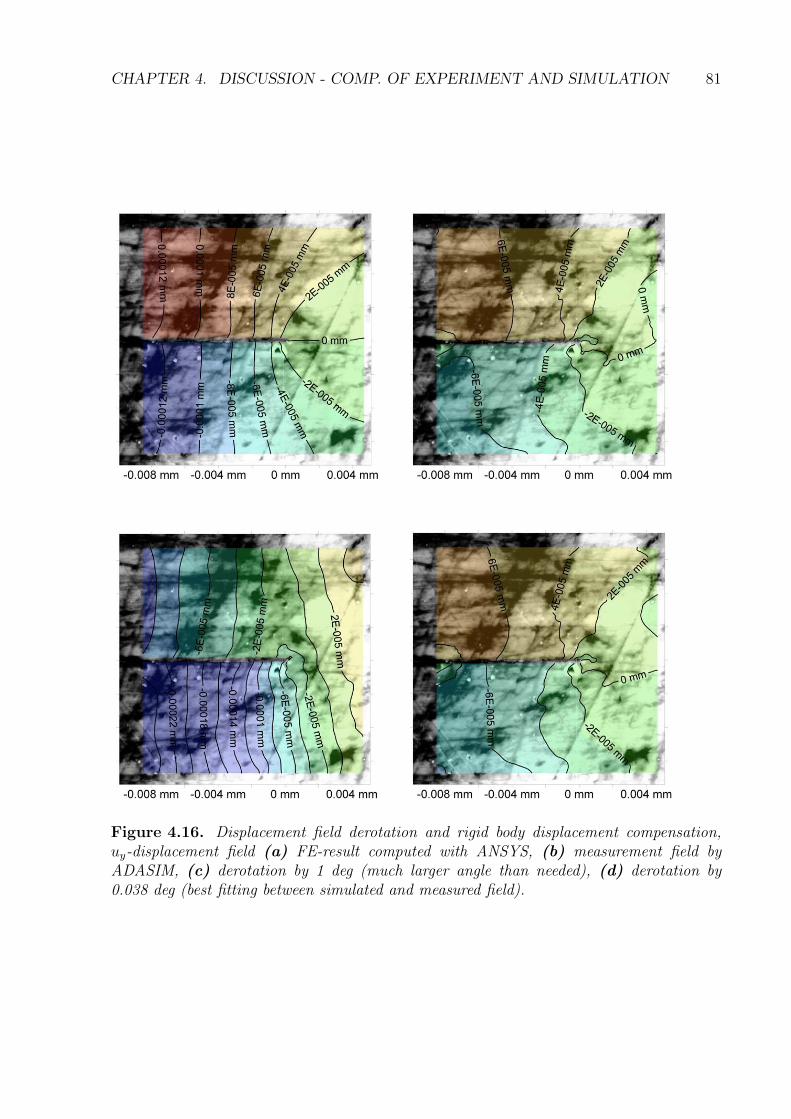
CHAPTER 4. DISCUSSION - COMP. OF EXPERIMENT AND SIMULATION 81
Figure 4.16. Displacement field derotation and rigid body displacement compensation,uy-displacement field (a) FE-result computed with ANSYS, (b) measurement field byADASIM, (c) derotation by 1 deg (much larger angle than needed), (d) derotation by0.038 deg (best fitting between simulated and measured field).

CHAPTER 4. DISCUSSION - COMP. OF EXPERIMENT AND SIMULATION 82
Determination of Material Properties
For the determination of material properties the verification algorithm has to be appliedto a pair of measured and simulated results. In this case the FE-results are varied andthe measured (or modified) field remain the same. FE-simulations are performed withdifferent Young’s moduli within a reasonable scope of values i.e. 2600 - 5000 MPa. Eachof the obtained FE-displacement fields is compared to the modified (derotated and rigidbody displacement corrected) measured field by means of the least square method.
Figure 4.17 illustrates the least square parameter versus the Young’s modulus of the FEsimulation. A minimum value of the least square parameter at a Young’s modulus of 3600MPa is indicating the best matching pair of displacement fields.
3000 4000 5000Young's Modulus [MPa]
0.16
0.2
0.24
0.28
0.32
Leas
t S
quar
e F
ittin
g
Figure 4.17. Determination of best fitting material model (Young’s modulus) at the min-imum of least square differences of displacements (here uy-field), best fit between FE andDIC for E = 3600 MPa.
Figure 4.18 shows the modified measured displacement field (a) and FE-based fields (b-c)where the best matching field is illustrated in (c).
The results of the verification algorithm clearly proof the capability of the adaptationconcept in combination with the verification algorithm. The applied verification strategyby comparison of measured and simulated displacement fields leads to a well defined bestmatching parameter set.
Unfortunately, the recursively derived Young’s modulus of 3600 MPa is not equivalent tothe measurements discussed in Sect. 3.2.5 where a value of 2800 MPa was determined. Areason for this can be that the relaxation test specimens for Young’s modulus determinationand the crack test CT-specimen are not manufactured from the same charge of material.Slightly different curing cycles can cause this deviation in material property. Moreover,unmodified cyanate ester resins tends to form a pre-stressed material configuration. Thisfact was indicated by the observation of cracks in the cured plates. Therefore, a homoge-neous material behavior cannot be guaranteed within the complete volume of the curedplates and the specimens. Especially at the surface of the plates the curing parameters are

CHAPTER 4. DISCUSSION - COMP. OF EXPERIMENT AND SIMULATION 83
different from that of the middle resulting in varying material properties over the thicknessof the plates.
Figure 4.18. Validation of FE-modeling by comparison of displacement fields with DICmeasurement, (a) ADASIM result for crack opening displacement field (derotated and rigidbody displacement corrected field), (b) FE field for non fitting simulation with E = 2800MPa, (c) FE field for best fit simulation with E = 3600 MPa.

CHAPTER 4. DISCUSSION - COMP. OF EXPERIMENT AND SIMULATION 84
4.6.5 Concluding Remarks on Adaptation Concept
The introduced adaptation strategy and measurement/simulation verification concept em-phasize its capability for the evaluation of micro- and nanocracks. Reliability testing andin-situ loading of newly developed micro- and nanoelectronics components supported byDIC measurements and FEA will give new insights in the material behavior on the micro-and nanoscale. Especially the potential in the determination of unknown material proper-ties qualifies the adaptation strategy as a powerful tool for future electronics and materialdesign.

Chapter 5
Conclusions and Outlook
In this thesis the principle of DIC-based displacement measurements extracted from in-situloading tests under the AFM is successfully applied to crack tip evaluation of a polymermaterial. The measurements were carried out in ambient air with a commercially availablescanning probe microscope equipped with specially designed loading stages.
The presented tests and results lead to the following conclusions:
• In general, the application of digital image correlation to SPM-based images is estab-lished as a technique for the extraction of displacements on the micro- and nanoscale.
• AFM topography images of surfaces with a defined roughness in the nm-range are wellsuited for the application of digital image correlation techniques and are, therefore,the basis for in-situ displacement measurements.
• System drifts induced by thermal drifts or piezoceramic based scanner instabilitiescan be eliminated. The correction for system drifts is achieved by fitting of correctionfunctions to mean displacements values.
• For scan sizes below 1 µm, the described SPM based displacement measurementtechnique is not qualified yet. Possible solutions for elimination of the arisen thermalinstabilities are the development of systems which compensate thermal drifts. An-other feasible approach would be a installation of thermal control units for the wholesystem or specific system components.
• Crack evaluation of micro- and nanocracks have to be supported by numerical sim-ulations. The introduced adaptation strategy is a possible method for a hybrid-typeevaluation of cracks and defects in electronic systems and MEMS/NEMS. A potentialis also seen for the testing and qualification of nanomaterials.
85

CHAPTER 5. CONCLUSIONS AND OUTLOOK 86
Outlook
The presented results serve as a basis for displacement measurements down to the nanoscale.As scanning probe microscopy is a cutting edge technology the application in the fields of(nano)-electronics, MEMS/NEMS, BIO-MEMS, and material science will be inevitable forfuture research. In the following, the trends emerging from several research fields showingdirect effect on the presented nanoDAC technique will be discussed briefly.
Nanomaterials
Design of nanomaterials is already a fundamental task for the development of tailoredstructural, active or passive components. Often the effects of incorporation of nanofillers,such as nanotubes or OLS on the macromechanical behavior are not understood. Thepresented nanoscale displacement measurement technique is a promising tool for qualitativeand quantitative description of these size-effects. However, further improvements of theaccuracy of the nanoDAC method is required to target the observation of objects in the10 nm range.
Interface problems
The growing number of passive and active ultrathin layers in microelectronic systems isbecoming a problem for experimental and FE-based reliability determination. A possiblesolution from the experimental point of view is newly developed DIC algorithms taken intoaccount the spatial variation of materials. By application of material based correlationzones the accuracy of method will be enhanced at the material interfaces. In combinationwith SPM or FIB/SEM experimental techniques an improvement of the nanoDAC methodcan be expected.
SPM developments
Arisen problems of stability will be overcome by the application of the actual SPM devel-opments. Higher scanning frequencies are a key for the experimental analysis of plasticor visco-plastic material classes and will reduce the errors introduced by thermal drifts.The problem of scanner creep and scanner nonlinearities caused by piezoceramic scanningdevices will be overcome by improved closed-loop scanning techniques. The applicationof capacitive components for scanning units has also a high potential for the accuracyenhancement of nanoscale displacement measurements.
Major improvements of the presented nanoDAC method are expected from the followingongoing developments of experimental techniques:
• application of fast scanning techniques in SPM equipment will reduce thermal drifts;
• combined SEM/SPM equipment improves the handling of the measurements;
• combined FIB/SEM tools will improve the specimen fabrication and will broaden theextracted information from the observed specimens;

CHAPTER 5. CONCLUSIONS AND OUTLOOK 87
• AFM topography image based 3D-DIC for 3D displacement fields is the key for aone-to-one comparison of finite element results and experimental approaches. With3-D displacement fields the correction for specimen tilt is becoming a solvable task.
Simulation
For future developments of microelectronic systems, MEMS and NEMS the importance ofthe combination of simulation and experiments will increase. The discussed adaptationstrategies will be improved by implementation of:
• weighting functions, to take into account the density of FE-meshes;
• automated recursive finite element parameter studies with stochastic parameter vari-ation;
• advanced concepts of automated derotation.
Parallel to these strategies emerging from classical mechanics approaches quantum mechan-ics will play an important role in the nanometer range. Nowadays, the existing quantummechanics simulation tools are beginning to expand their capabilities from molecular mod-eling towards meso-type material descriptions. The implementation of homogenizationtechniques is believed to close the technological gap between the micro- and nanoworld.The term homogenization is understood as the numerical determination of a model de-scribing a representative volume of bulk material. Thereby, the spacial distribution of fillerparticles or different material phases are taken into account. The results of the homoge-nization will be employed as input data for standard finite element codes.

Bibliography
[1] R. Bashir. Biological Mediated Assembly of Artificial Nanostructures and Microstruc-tures. In W.A. Goddard, D.W. Brenner, S.E. Lyschevski, and G.J. Iafarte, editors,Handbook of Nanoscience, Engineering, and Technology. CRC Press, Boca Raton,2003.
[2] D. Vogel, A. Schubert, W. Faust, R. Dudek, and B. Michel. MicroDAC - a Novel Ap-proach to Measure In Situ Deformation Fields of Microscopic Scale. MicroelectronicsReliability, 36(11-12):1939–1942, 1996.
[3] M. Bauer and J. Bauer. Aspects of the Kinetics, Modelling and Simulation of Net-work Build-Up During Cyanate Ester Cure. In I. Hamerton, editor, Chemistry andTechnology of Cyanate Ester Resins, pages 58–86. Chapman & Hall, 1994.
[4] G.-M. Kim and G.H. Michler. Micromechanical Deformation Processes in Toughenedand Particle-Filled Semicrystalline Polymers: Part 1. Characterization of Deforma-tion Processes in Dependence on Phase Morphology. Polymer, 39(23):5689–5697,1998.
[5] J.U. Starke, G.H. Michler, W. Grellmann, S. Seidler, M. Gahleitner, J. Fiebig, andE. Nezbedova. Fracture Toughness of Polypropylene Copolymers: Influence of Inter-particle Distance and Temperature. Polymer, 39(1):75–82, 1998.
[6] D. Baither, F. Ernst, T. Wagner, M. Ruhle, M. Bartsch, and U. Messerschmidt.Micromechanisms of Fracture in NiAl Studied by In Situ Straining Experiments inan HVEM. Intermetallics, 7:479–489, 1999.
[7] J. Guan, C. Wang, and W. Chu. Atomic Structure of Loaded Crack Tip by AFM.Scripta Materialia, 39(9):1211–1214, 1998.
[8] Y.H. Lu, Y.G. Zhang, L.J. Qiao, Y.-B. Wang, C.Q. Chen, and W.Y. Chu. In-SituTEM Study of Fracture Mechanisms of Polysynthetically Twinned (PST) Crystalsof TiAl Alloys. Material Science and Engineering A, 289(1-2):91–98, 2000.
[9] J.X. Li, W.Y. Chu, Y.B. Wang, and L. J. Qiao. In Situ TEM Study of StressCorrosion Cracking of Austenitic Stainless Steel. Corrosion Science, 45(7):1355–1365, 2003.
[10] L. Cretegny and A. Saxena. AFM Characterization of the Evolution of SurfaceDeformation During Fatigue in Polycrystalline Copper. Acta Materialia, 49:3755–3765, 2001.
88

BIBLIOGRAPHY 89
[11] L. Cretegny and A. Saxena. Evolution of Surface Deformation During Fatigue ofPH 13-8 Mo Stainless Steel Using Atomic Force Microscopy. Fatigue & Fracture ofEngineering Materials & Structures, 25(3):305–314, 2002.
[12] M.S. Bobji and B. Bushan. Atomic Force Microscopic Study of the Micro-Crackingof Magnetic Thin Films under Tension. Scripta Materialia, 44(1):37–42, 2001.
[13] M.S. Bobji and B. Bushan. In Situ Microscopic Surface Characterization Studies ofPolymeric Thin Films During Tensile Deformation Using Atomic Force Microscopy.Journal of Materials Research, 16(3):844–855, 2001.
[14] T. Kinoshita. Stress Singularity Near the Crack-Tip in Silicon Carbide: Investigationby Atomic Force Microscopy. Acta Materialia, 46(11):3963–3974, 1998.
[15] K. Komai, K. Minoshima, and S. Inoue. Fracture and Fatigue Behavior of SingleCrystal Silicon Microelements and Nanoscopic AFM Damage Evaluation. Microsys-tem Technologies, 5(1):30–37, 1998.
[16] C. Marieta, M. del Rio, I. Harismendy, and I. Mondragon. Effect of the Cure Tem-perature on the Morphology of a Cyanate Ester Resin Modified with a Thermo-plastic: Characterization by Atomic Force Microscopy. European Polymer Journal,36(7):1445–1454, 2000.
[17] C. Marieta, P.M. Remiro, G. Garmendia, I. Harismendy, and I. Mondragon. AFMApproach Toward Understanding Morphologies in Toughened Thermosetting Matri-ces. European Polymer Journal, 39(10):1965–1973, 2003.
[18] F. Creuzet and E. Guilloteau. An AFM Study of Key Phenomena Involved in theFracture of Glass. Verre, 1(6):11–13, 1995.
[19] M. Goken, H. Vehoff, and P. Neumann. Atomic Force Microscopy Investigationsof Loaded Crack Tips in NiAl. Journal of Vacuum Science and Technology B,14(2):1157–1161, 1996.
[20] F. Thome, M. Goken, and H. Vehoff. Study of the Fracture Behavior in Soft andHard Oriented NiAl Single Crystals by AFM. Intermetallics, 7(3-4):491–499, 1999.
[21] M. Goken, M. Maßmann, F. Thome, and H. Vehoff. Microscopic Fracture Behaviorof Single Crystalline Intermetallics. In Structural Intermetallics 1997. Proceedingsof the Second International Symposium on Structural Intermetallics, pages 641–648,1996.
[22] H. Vehoff, P. Ochmann, M. Goken, and M. Große Gehling. Deformation Processesat Crack Tips in NiAl Single- and Bicrystals. Material Science and Engineering A,239-240(1-2):378–385, 1997.
[23] M. Goken, F. Thome, and H. Vehoff. Study of Crack Tip Deformation in FeAl andNiAl Crystals with Optical Interference Microscopy and Atomic Force Microscopy.Philosophical Magazine A, 82(17-18):3241–3250, 2002.

BIBLIOGRAPHY 90
[24] U. Rabe, K. Janser, and W. Arnold. Vibrations of Free and Surface-Coupled AtomicForce Microscope Cantilevers: Theory and Experiment. Review of Scientific Instru-ments, 67(9):3281–3293, 1996.
[25] E. Chilla, T. Hesjedal, and H.J. Frohlich. Scanning Acoustic Force Microscope De-tection of SAWs. In IEEE Ultrasonics Symposium. Proceedings, pages 363–366, 1994.
[26] U. Rabe, S. Amelio, E. Kester, V. Scherer, S. Hirsokorn, and W. Arnold. Quan-tative Determination of Contact Stiffness Using Atomic Force Acoustic Microscopy.Ultrasonics, 38(1-8):430–437, 2000.
[27] O.V. Kolosov, M.R. Castell, C.D. Marsh, G.A.D Briggs, T.I. Kamins, and R.S.Williams. Imaging the Elastic Nanostructure of Ge Island by Ultrasonic Force Mi-croscopy. Physical Review Letters, 81(5):1046–1049, 1998.
[28] K. Yamanaka. UFM Observation of Lattice Defects in Highly Oriented PyroliticGraphite. Thin Solid Films, 273(1-2):116–121, 1996.
[29] C.J. Druffner and S. Sathish. Improving Atomic Force Microscopy with the Adapta-tion of Ultrasonic Force Microscopy. In Proc. SPIE Vol. 4703, Nondestructive Eval-uation and Reliability of Micro- and Nanomaterial Systems, pages 105–113, 2002.
[30] K. Porfyrakis, H.E. Assender, and I.M. Robinson. The Interrelationship Between Pro-cessing Conditions, Microstructure and Mechanical Properties for Injection MouldedRubber-Toughened Poly(methyl methacrylate) (RTPMMA) Samples. Polymer,43(17):4769–4781, 2002.
[31] A. Kuske and G. Robertson. Photoelastic Stress Analysis. Wiley, London, 1974.
[32] E. O’Brien. A Review of Current Research in Photoelasticity. In Photo-Mecanique98, pages 49–55, 1998.
[33] T.Y. Chen. Digital Photoelasticity. In P.K. Rastogi, editor, Photomechanics, pages197–232. Spinger, 2000.
[34] D. Coker, A.J. Rosakis, and A. Needleman. Dynamic Crack Growth Along a Poly-mer Composite-Homalite Interface. Journal of the Mechanics and Physics of Solids,51(3):425–460, 2003.
[35] A. Asundi, H. Xie, J. Yu, and Z. Zhong. Phase-Shifting AFM Moire Method. InProc. SPIE Vol. 4448, Optical Diagnostics for Fluids, Solids, and Combustion, pages102–110, 2001.
[36] P.F. Luo, Y.J. Chao, M.A. Sutton, and W.H. Peters. Accurate Measurement ofThree-Dimensional Deformations in Deformable and Rigid Bodies Using ComputerVision. Experimental Mechanics, 33(2):123–132, 1993.
[37] A. Tatschl and O. Kolednik. A New Tool for the Experimental Characterization ofMicro-Plasticity. Materials Science and Engineering A, 339(1-2):265–280, 2002.
BIBLIOGRAPHY 91
[38] M.A. Sutton, W.J. Wolters, W.H. Peters, W.F. Ranson, and S.R. McNeill. Deter-mination of Displacements Using an Improved Digital Image Correlation Method.Image Vision Computing, 1(3):133–139, 1983.
[39] F.-P. Chiang. Moire and Speckle Methods Applied to Elastic-Plastic Fracture Me-chanics. In J.S. Epstein, editor, Experimental Techniques in Fracture, pages 291–325.VCH Publishers, 1993.
[40] K. Matsumoto and M. Takashima. Improvements on Moire Technique for In-PlaneDeformation Measurements. Applied Optics, 12(4):858–864, 1973.
[41] D. Post, B. Han, and P. Ifju, editors. High Sensitivity Moire. Springer, New York,1994.
[42] B. Michel and R. Kuehnert. Mikro-Moire-Methode und MikroDAC-Verfahren an-wenden. Materialprufung, 38(7/8):311–315, 1996.
[43] D.T. Read and J.W. Dally. Theory of Electron Beam Moire. Journal of Research ofthe National Institute of Standards and Technology, 101(1):47–61, 1996.
[44] H. Xie, A. Asundi, C.G. Boay, L. Yungguang, J. Yu, Z. Zhaowei, and B. K.A Ngoi.High Resolution AFM Scanning Moire Method and its Application to the Micro-Deformation in the BGA Electronic Package. Microelectronics Reliability, 42:1219–1227, 2002.
[45] A. Asundi, X. Huimin, L. Chongxiang, C.G. Boay, and O.K. Eng. Micro-MoireMethods - Optical and Scanning Techniques. In Proc. of SPIE Vol. 4416, OpticalEngineering for Sensing and Nanotechnology (ICOSN 2001), pages 54–57, 2001.
[46] Y. Xing, F. Dai, and W. Yang. Experimental Study About Nano-Deformation FieldNear Quasi-Cleavage Crack Tip. Science in China, Series A (Mathematics, Physics,Astronomy), 43(9):963–968, 2000.
[47] H. Xie, B. Li, R. Geer, B. Xu, and J. Castracane. Focused Ion Beam Moire Method.Optics and Lasers in Engineering, 40:163–177, 2003.
[48] F.-P. Chiang. A Family of 2D and 3D Experimental Stress Analysis Technique UsingLaser Speckle. Solid Mechanics Archives, 3(1):1–32, 1978.
[49] R.S. Sirohi and F.S. Chau, editors. Optical Methods of Measurement - WholefieldTechniques. Marcel Dekker, New York, 1999.
[50] W.H. Peters and W.F. Ranson. Digital Imaging Techniques in Experimental StressAnalysis. Optical Engineering, 21(3):427–431, 1982.
[51] M.A. Sutton, M. Cheng, W.H. Peters, Y.J. Chao, and S.R. McNeill. Applicationof an Optimized Digital Image Correlation Method to Planar Deformation Analysis.Image and Vision Computing, 4(3):143–150, 1986.

BIBLIOGRAPHY 92
[52] H.A. Bruck, S.R. McNeill, M.A. Sutton, and Peters W.H. Digital Image CorrelationUsing Newton-Raphson Method of Partial Differential Correlation. ExperimentalMechanics, 29(3):261–267, 1989.
[53] M.A. Sutton, S.R. McNeill, J.D. Helm, and M.L. Boone. Measurement of Crack TipOpening Displacement and Full-Field Deformations During Fracture of AerospaceMaterials Using 2d and 3d Image Correlation Methods. In A. Lagarde, editor, IUTAMSymposium on Advanced Optical Methods and Applications in Solid Mechanics, pages571–580, 2000.
[54] T.C. Chu, W.F. Ranson, M.A. Sutton, and W.H. Peters. Application of Digital-Image-Correlation Techniques to Experimental Mechanics. Experimental Mechanics,25(3):232–244, 1985.
[55] Y.-J. Chao and M.A. Sutton. Accurate Measurement of Two- and Three-DimensionalSurface Deformations for Fracture Specimens by Computer Vision. In J.S. Epstein,editor, Experimental Techniques in Fracture, pages 59–93. VCH Publishers, 1993.
[56] J. Liu, J. Lyons, M. Sutton, and A. Reynolds. Experimental Characterization ofCrack Tip Deformation Fields in Alloy 718 at High Temperatures. Journal of Engi-neering Materials and Technology, 120(1):71–78, 1998.
[57] J. Gonzalez and W.G. Knauss. Strain Inhomogeneity and Discontinuous CrackGrowth in a Particulate Composite. Journal of the Mechnanics and Physics of Solids,46(10):1981–1995, 1998.
[58] W.D. Lockwood and A.P. Reynolds. Use and Verification of Digital Image Correlationfor Automated 3-D Surface Characterization in the Scanning Electron Microscope.Materials Characterization, 42(2-3):123–134, 1999.
[59] M.G.D. Geers, R. de Borst, and T. Peijs. Mixed Numerical-Experimental Identifi-cation of Non-Local Characteristics of Random-Fibre-Reinforced Composites. Com-posites Science and Technology, 59(10):1569–1578, 1999.
[60] J. Lambros, A. Narayanaswamy, M.H. Santare, and G.J. Anlas. Manufacture andTesting of a Functionally Graded Material. Journal of Engineering Materials andTechnology, 121(4):488–493, 1999.
[61] A.-F. Bastawros and A.G. Evans. Deformation Heterogeneity in Cellular Al Alloys.Advanced Engineering Materials, 2(4):210–214, 2000.
[62] A.-F. Bastawros, H. Bart-Smith, and A.G. Evans. Experimental Analysis of Deforma-tion Mechanisms in a Closed-Cell Aluminum Alloy Foam. Journal of the Mechanicsand Physics of Solids, 48(2):301–322, 2000.
[63] H.W. Schreier, J.R. Braasch, and M.A. Sutton. Systematic Errors in Digital ImageCorrelation Caused by Intensity Interpolation. Optical Engineering, 39(11):2915–2921, 2000.

BIBLIOGRAPHY 93
[64] I. Chasiotis and W.G. Knauss. A New Microtensile Tester for the Study of MEMSMaterials with the Aid of Atomic Force Microscopy. Experimental Mechanics,42(1):51–57, 2002.
[65] J. Abanto-Bueno and J. Lambros. Investigation of Crack Growth in FunctionallyGraded Materials Using Digital Image Correlation. Engineering Fracture Mechanics,69(14-16):1695–1711, 2002.
[66] D.L. Davidson. Micromechanics Measurement Techniques for Fracture. In J.S. Ep-stein, editor, Experimental Techniques in Fracture, pages 41–57. VCH Publishers,1993.
[67] D. Vogel, J. Auersperg, A. Schubert, B. Michel, and H. Reichl. Deformation Analysison Flip Chip Solder Interconnects by MicroDAC. In Design and Reliability of Sol-ders and Solder Interconnections. Proceedings of a Symposium held during the TMSAnnual Meeting, pages 429–438, 1997.
[68] D. Vogel, J. Simon, A. Schubert, and B. Michel. High Resolution DeformationMeasurement on CSP and Flip Chip. In Fourth VLSI Packaging Workshop of Japan.Technical Digest, pages 84 – 86, Kyoto, 1998.
[69] E. Soppa, P. Doumalin, P. Binkele, T. Wiesendanger, B. Bornert, and S. Schmauder.Experimental and Numerical Characterisation on In-Plane Deformation in Two-Phase Materials. Computational Materials Science, 21(3):261–275, 2001.
[70] G. Vendroux, N. Schmidt, and W.G. Knauss. Submicron Deformation Field Measure-ments. 3. Demonstration of Deformation Determinations. Experimental Mechanics,38(3):154–160, 1998.
[71] Y. Huang. Scanning Tunneling Microscopy and Digital Image Correlation inNanomechanics Investigations. Ph.D. thesis, California Institute of Technology,Pasadena, 2001.
[72] W.G. Knauss, I. Chasiotis, and Y. Huang. Mechanical Measurements at the Micronand Nanometer Scales. Mechanics of Materials, 35(3-6):217–231, 2003.
[73] D. Vogel and B. Michel. Microcrack Evaluation for Electronics Components byAFM nanoDAC Deformation Measurement. In Proceedings of the 2001 1st IEEEConference on Nanotechnology. IEEE-NANO 2001, pages 309–312, 2001.
[74] D. Vogel, J. Keller, A. Gollhardt, and B. Michel. Evaluating Microdefect Structuresby AFM based Deformation Measurement. In Proc. of SPIE Vol. 5045, TestingReliability, and Application of Micro- and Nano-Materials Systems, pages 1–12, 2003.
[75] J. Keller, D. Vogel, A. Schubert, and B. Michel. Displacement and Strain FieldMeasurements from SPM Images. In B. Bhushan, H. Fuchs, and S. Hosaka, editors,Applied Scanning Probe Methods, pages 253–276. Springer, 2004.
BIBLIOGRAPHY 94
[76] J. Keller, A. Gollhardt, D. Vogel, and B. Michel. Characterization of Microcracks byApplication of Digital Image Correlation to SPM Images. In Proceedings of SPIE 11thAnnual International Symposium on Smart Structures and Materials, 14-18 March,2004, page to be published, 2004.
[77] G. Vendroux and W.G. Knauss. Submicron Deformation Field Measurements. 2.Improved Digital Image Correlation. Experimental Mechanics, 38(2):86–92, 1998.
[78] M.A. Sutton, S.R. McNeill, J. Jang, and M. Babai. Effects of Subpixel Image Restora-tion on Digital Correlation Error Estimates. Optical Engineering, 27(10):870–877,1988.
[79] G. Vendroux and W.G. Knauss. Submicron Deformation Field Measurements. 1.Developing a Digital Scanning Tunneling Microscope. Experimental Mechanics,38(1):18–23, 1998.
[80] D. Vogel, J. Auersperg, and B. Michel. Characterization of Electronic PackagingMaterials and Components by Image Correlation Methods. In Proc. of SPIE, Ad-vanced Photonic Sensors and Applications II, Nov. 27-30 2001, Singapore, volume4596, pages 237–247, 2001.
[81] M. Dost, E. Kieselstein, and R. Erb. Displacement Analysis by Means of GreyScale Correlation at Digitized Images and Image Sequence Evaluation for Micro-and Nanoscale Applications. Micromaterials and Nanomaterials, 1(1):30–35, 2002.
[82] T.L. Anderson. Fracture Mechanics: Fundamentals and Applications. CRC Press,2nd edition, 1995.
[83] D. Gross. Bruchmechanik. Springer, 1996.
[84] American Society for Testing and Materials. ASTM D5045, Standard Test Meth-ods for Plane-Strain Fracture Toughness and Strain Energy Release Rate of PlasticMaterials , 1999.
[85] G.R. Irwin. Onset of Fast Crack Propagation in High Strength Steel and AluminumAlloys. In Sagamore Research Conference Proceedings, volume 2, pages 289–305,1956.
[86] J.R. Rice. A Path Independent Integral and the Approximate Analysis of StrainConcentration by Notches and Cracks. Journal of Applied Mechanics, 35:379–386,1968.
[87] D.M. Parks. A Stiffness Derivative Finite Element Technique for Determination ofCrack Tip Stress Intensity Factors. International Journal of Fracture, 10(4):487–502,1974.
[88] T.K. Hellen. On the Method of Virtual Crack Extensions. International Journal forNumerical Methods in Engineering, 9(1):187–207, 1975.

BIBLIOGRAPHY 95
[89] H.G. deLorenzi. On the Energy Release Rate and the J-Integral of 3-D Crack Con-figurations. International Journal of Fracture, 19(3):183–193, 1982.
[90] H.G. deLorenzi. Energy Release Rate Calculations by Finite Element Method. En-gineering Fracture Mechanics, 21(1):129–143, 1985.
[91] H.B. Ghavifekr. Einsatz bruchmechanischer Integralkonzepte zur thermomecha-nischen Zuverlassigkeitsbewertung in der mikroelektronischen Aufbau- und Ver-bindungstechnik. Ph.D. Thesis, Technische Universitat Berlin, Berlin, 2003.
[92] N.L. Goldman and J.W. Hutchinson. Fully Plastic Crack Problems: The Center-Cracked Strip under Plane Strain. International Journal of Solids and Structures,11(5):575–591, 1975.
[93] J.D. Landes and J.A. Begley. A Fracture Mechanics Approach to Creep CrackGrowth. In ASTM STP, 590, pages 128–148. American Society for Testing andMaterials, 1976.
[94] K. Kishimoto, S. Aoki, and M. Sakata. On the Path Independent Integral - J .Engineering Fracture Mechanics, 13(4):841–850, 1980.
[95] S.N. Atluri. Path-Independent Integrals in Finite Elasticity and Inelasticity, withBody Forces, Inertia, and Arbitrary Crack-Face Conditions. Engineering FractureMechanics, 16(3):341–364, 1982.
[96] S.N. Atluri, T. Nishioka, and M. Nakagaki. Incremental Path-Independent Inte-grals in Inelastic and Dynamic Fracture Mechanics. Engineering Fracture Mechanics,20(2):209–244, 1984.
[97] G. Menges, E. Haberstroh, W. Michaeli, and E. Schmachtenberg. WerkstoffkundeKunststoffe. Hanser, 5. edition, 2002.
[98] A.J. Kinloch and R.J. Young. Fracture Behaviour of Polymers. Elsevier AppliedScience Publishers, London, 1983.
[99] G.H. Michler. Kunststoff-Mikromechanik: Deformations- und Bruchmechanismen.Hanser, Munchen, 1992.
[100] I. Hamerton. Introduction to Cyanate Ester Resins. In I. Hamerton, editor, Chem-istry and Technology of Cyanate Ester Resins, pages 1–6. Chapman & Hall, 1994.
[101] C.P.R. Nair, D. Mathew, and K.N. Ninan. Cyanate Ester Resins, Recent Develop-ments. Advances in Polymer Science, 155:1–99, 2001.
[102] A.W. Snow. The Synthesis, Manufacture and Characterization of Cyanate EsterMonomers. In I. Hamerton, editor, Chemistry and Technology of Cyanate EsterResins, pages 7–57. Chapman & Hall, 1994.

BIBLIOGRAPHY 96
[103] S.L. Simon and J.K. Gillham. Cure Kinetics of a Thermosetting Liquid Dicyanate Es-ter Monomer/High-Tg Polycyanurate Material. Journal of Applied Polymer Science,47(3):461–485, 1993.
[104] J. Bauer and M. Bauer. Cyanate Ester Based Resin Systems for Snap-Cure Appli-cations. Microsystem Technologies, 8:58–62, 2002.
[105] D.A. Shimp and B. Chin. Electrical Properties of Cyanate Ester Resins and theirSignificance for Applications. In I. Hamerton, editor, Chemistry and Technology ofCyanate Ester Resins, pages 230–281. Chapman & Hall, 1994.
[106] T. Fang and D.A. Shimp. Polycyanate Esters: Science and Applications. Progressin Polymer Science, 20(1):61–118, 1995.
[107] D.A. Shimp. Applications of Cyanate Ester (CE) Resins. Polymeric Material Scienceand Engineering, 71:561–562, 1994.
[108] A.J. Kinloch and A.C. Taylor. The toughening of cyanate-ester polymers. Journalof Materials Science, 38:65–79, 2003.
[109] S. Ganguli, D. Dean, K. Jordan, G. Price, and R. Vaia. Mechanical Propertiesof Intercalated Cyanate Ester-Layered Silicate Nanocomposites. Polymer, 44:1315–1319, 2003.
[110] Y.M. Haddad. Viscoelasticity of Engineering Materials. Chapman & Hall, London,1995.
[111] J.D. Ferry. Viscoelastic Properties of Polymers. Wiley, New York, 3rd edition, 1980.
[112] J.D. Ferry, R.F. Landel, and M.L. Williams. Extensions of the Rouse Theory ofViscoelastic Properties to Undiluted Linear Polymers. Journal of Applied Physics,26(4):359–362, 1955.
[113] Deutsches Institut fur Normung. DIN 53504, Prufung von Kautschuk und Elas-tomeren; Bestimmung von Reißfestigkeit, Zugfestigkeit, Reißdehnung und Span-nungswerten im Zugversuch. Beuth, Ausgabe: 1994-05.
[114] C. Uhlig, O. Kahle, B. Wieneke, and M. Bauer. A New Method for the AutomaticDetermination of Fracture Toughness of Polymers. Forum der Forschung, 5(11):50–53, 2000. BTU Cottbus.
[115] J. Keller, C. Uhlig, O. Kahle, B. Wieneke, B. Michel, and M. Bauer. OpticalCrack Tracing - A New Method for Automatic Fracture Toughness Measurement.In Werkstoffwoche-Partnerschaft, editor, Materials Week 2000 and 2001, Proceed-ings, Frankfurt, 2002. Werkstoff-Informationsgesellschaft.
[116] C. Uhlig, O. Kahle, B. Wieneke, and M. Bauer. Optical Crack Tracing - A NewMethod for the Automatic Determination of Fracture Toughness for Crack Initiationand Propagation. In Proceedings of the 3rd International Micro Materials Conference,Berlin, 17-19 April 2000, pages 618–629, 2000.

BIBLIOGRAPHY 97
[117] C. Uhlig, O. Kahle, B. Wieneke, and M. Bauer. Optical Crack Tracing - A NewMethod for the Automatic Determination of Fracture Toughness for Crack Initia-tion and Propagation. In 3rd Int. Conf. Mechanics of Time Dependent Materials,Erlangen, Sept. 17-20, 2000, 2000.
[118] G. Binning, H. Rohrer, C. Gerber, and E. Weibel. Surface Studies by ScanningTunneling Microscopy. Physical Review Letters, 49(5):57–61, 1982.
[119] G. Binning, C.F. Quate, and C. Gerber. Atomic Force Microscope. Physical ReviewLetters, 56(9):930–933, 1986.
[120] B. Bhushan, editor. Springer Handbook of Nanotechnology. Springer, 2004.
[121] ThermoMicroscopes, Sunnyvale, California. User’s Guide to Autoprobe CP and M5,August 2000.
[122] Y. Martin, C.C. Williams, and H.K. Wickramasinghe. Atomic Force Microscope-Force Mapping and Profiling on a sub 100-A Scale. Journal of Applied Physics,61(10):4723–4729, 1987.
[123] D. Sarid and V. Elings. Review of Scanning Force Microscopy. Journal of VacuumScience and Technology B, 9(2):431–437, 1991.
[124] Q. Zhong, D. Inniss, K. Kjoller, and V.B. Elings. Fractured Polymer/Silica FiberSurface Studied by Tapping Mode Atomic Force Microscopy. Surface Science Letters,290:L688–L692, 1993.
[125] S.N. Magonov and M.-H. Whangbo. Surface Analysis with STM and AFM: Experi-mental and Theoretical Aspects of Image Analysis. VCH, Weinheim, 1996.
[126] P. West and N. Starostina. A Guide to AFM Image Artifacts. Pacific Nanotechnology,http://www.pacificnanotech.com/afm-artifacts.html.
[127] D.T. Nguyen. Messgenauigkeit von nanoDAC - Verschiebungsfeldmessungen im Scan-ning Force Microscope. Master Thesis, Technische Fachhochschule Berlin, Berlin,2003.
[128] B. Wunderle, J. Auersperg, V. Groer, E. Kaulfersch, O. Wittler, and B. Michel. Mod-ular Parametric Finite Element Modelling for Reliability-Studies in Electronic andMEMS Packaging. Proc. of Symposium on Design, Test, Integration and Packagingof MEMS/MOEMS, May 5-7, Cannes, France, pages 335–340, 2003.
[129] SAS IP. ANSYS 7.0 Documentation, 2002.
[130] Image Instruments. ADASIM User Manual, ADASIM Version 1.1. Image Instru-ments GmbH, Chemnitz, Germany, 2004.
[131] D. Vogel, V. Grosser, A. Schubert, and B. Michel. MicroDAC Strain Measurementfor Electronics Packaging Structures. Optics and Lasers in Engineering, 36:195–211,2001.

Lebenslauf
Name: Jurgen Keller
Geburtstag: 10.06.1972
Geburtsort: Bad Sobernheim
1978 – 1982 Grundschule in Monzingen
1982 – 1991 Staatliches Gymnasium in Bad Sobernheim
05/1991 Allgemeine Hochschulreife
1991 – 1992 Grundwehrdienst, JaboG 34, Bad Sobernheim
1992 – 1999 Studium Maschinenbau und Verfahrenstechnik an der Univer-sitat Kaiserslautern
05/1996 – 10/1996 Studium an der University of Bristol, England
11/1998 – 05/1999 Diplomarbeit am Shonan Institute of Technology, Fujisawa,Japan
06/1999 Abschluss des Studiums als Diplom-Ingenieur, Thema der Di-plomarbeit:
”Friction and Wear Properties of Continuous-Fibre
Ceramic-Matrix Composites“, Universitat Kaiserslautern, durch-gefuhrt am Shonan Institute of Technology, Fujisawa, Japan
10/1999 – 2003 Wissenschaftlicher Mitarbeiter am Lehrstuhl fur Polymerwerk-stoffe der Brandenburgischen Technischen Universitat Cottbus
seit 10/1999 Promotion mit dem Thema:”Micro- and Nanoscale Characteri-
zation of Polymeric Materials by Means of Digital Image Cor-relation Techniques“ am Lehrstuhl fur Polymermaterialien derBrandenburgischen Technischen Universitat, Cottbus, in Zusam-menarbeit mit dem Fraunhofer Institut fur Zuverlassigkeit undMikrointegration, Berlin
seit 06/2003 Tatigkeit als Entwicklungsingenieur Micro- and Nanomaterialsin der AMIC Angewandte Micro-Messtechnik GmbH, Berlin
98

Erklarung
Ich versichere, dass ich die von mir vorgelegte Dissertation selbstandig und ohne unzulassigeHilfe angefertigt, die benutzten Quellen und Hilfsmittel vollstandig angegeben und dieStellen der Arbeit – einschliesslich Tabellen und Abbildungen – die anderen Werken imWortlaut oder dem Sinn nach entnommen sind, in jedem Einzelfall als Entlehnung kenntlichgemacht habe, dass diese Dissertation noch keiner anderen Fakultat zur Prufung vorgelegenhat, dass sie noch nicht veroffentlicht worden ist, sowie dass mit der Veroffentlichung derDissertation bestehende Schutzrechte nicht verletzt werden.
Die Bestimmungen der geltenden Promotionsordnung sind mir bekannt. Die von mir vorge-legte Dissertation ist von Frau Prof. Dr. Monika Bauer und Herrn Prof. Dr. Bernd Michelbetreut worden.
Jurgen Keller
99