MICRO AND MACRO-LEVEL APPROACHES FOR

ASSESSING THE VALUE OF IRRIGATION WATER

Robert C. Johansson

World Bank Policy Research Working Paper 3778, December 2005 The Policy Research Working Paper Series disseminates the findings of work in progress to encourage the exchange of ideas about development issues. An objective of the series is to get the findings out quickly, even if the presentations are less than fully polished. The papers carry the names of the authors and should be cited accordingly. The findings, interpretations, and conclusions expressed in this paper are entirely those of the authors. They do not necessarily represent the view of the World Bank, its Executive Directors, or the countries they represent. Policy Research Working Papers are available online at http://econ.worldbank.org.

This paper is a product of the study “Macro-Micro Linkages of Irrigation Water Management.” The Research Support Budget of the World Bank and Development Economics Research Group (DECRG) provided necessary funding. The study is being carried out by the Agriculture and Rural Development Department (ARD) at the World Bank. The Study Core Team includes Ariel Dinar (Team Leader, ARD, World Bank), Terry Roe (University of Minnesota, USA), Yacov Tsur (Hebrew University of Jerusalem, Israel) and Xinshen Diao (IFPRI, USA). Country consultants include Rachid Doukkali (Institute Hassan II, Morocco), Rashid Hassan (University of Pretoria, South Africa) and Erol Cakmak (Middle East Technical University, Turkey). Robert C. Johansson is an agricultural economist at the Economic Research Service, United States Department of Agriculture. This research was initiated while Dr. Johansson was a graduate student at the University of Minnesota. Comments on an earlier draft by Noel Gollehon, Glenn Schaible, Terry Roe, Yacov Tsur and Ariel Dinar are greatly appreciated. The views and opinions expressed herein are those of the author and not necessarily those of the Economic Research Service or the U.S. Department of Agriculture.

WPS3778

Pub

lic D

iscl

osur

e A

utho

rized

Pub

lic D

iscl

osur

e A

utho

rized

Pub

lic D

iscl

osur

e A

utho

rized

Pub

lic D

iscl

osur

e A

utho

rized

Pub

lic D

iscl

osur

e A

utho

rized

Pub

lic D

iscl

osur

e A

utho

rized

Pub

lic D

iscl

osur

e A

utho

rized

Pub

lic D

iscl

osur

e A

utho

rized

ii

CONTENTS ABSTRACT .................................................................................................................................................................3 SUMMARY..................................................................................................................................................................4 1. INTRODUCTION – WHY IS WATER VALUABLE?.......................................................................................6

1.1 WATER ALLOCATION POLICIES ...........................................................................................................................7 1.2 MACROECONOMIC POLICIES ................................................................................................................................8 1.3 SCOPE OF REVIEW................................................................................................................................................8

2. VALUING IRRIGATION WATER – BACKGROUND ....................................................................................9 2.1 IRRIGATION WATER DEMAND..............................................................................................................................9 2.2 IRRIGATION WATER SUPPLY..............................................................................................................................14 2.3 OBSERVING THE VALUE OF WATER...................................................................................................................17

3. ECONOMETRIC APPROACHES.....................................................................................................................19 3.1 CROP-WATER PRODUCTION FUNCTIONS............................................................................................................19 3.2 REDUCED FORM APPROACHES...........................................................................................................................20 3.3 MULTICROP SETTING.........................................................................................................................................21 3.4 CONTROLLING FOR INEFFICIENCY......................................................................................................................22 3.5 INCOMPLETE DATA............................................................................................................................................23

4. MATHEMATICAL PROGRAMMING APPROACHES .................................................................................24 4.1 LINEAR AND NONLINEAR MATHEMATICAL PROGRAMMING ..............................................................................24 4.2 POSITIVE MATHEMATICAL PROGRAMMING (PMP)............................................................................................26 4.3 RESTRICTED-EQUILIBRIUM MODELS .................................................................................................................27 4.4 INTEGRATED MODELS........................................................................................................................................28

5. GENERAL EQUILIBRIUM APPROACHES....................................................................................................29 5.1 MACROECONOMY ..............................................................................................................................................31 5.2 PRODUCTION INPUTS.........................................................................................................................................32 5.3 SECOND-BEST CONSIDERATIONS.......................................................................................................................34

6. LINKAGES BETWEEN MICRO AND MACRO ECONOMIES ...................................................................35 6.1 MICROECONOMY ...............................................................................................................................................36 6.2 MACROECONOMY ..............................................................................................................................................39 6.3 THE ENVIRONMENT ..........................................................................................................................................41

7. CONCLUSIONS...................................................................................................................................................43 REFERENCES ..........................................................................................................................................................46

3

Abstract

Many countries are reforming their economies and setting macro policies that have direct and indirect impact on the performance of the irrigation sector. One reason for the movement towards reform in the water sector across countries is that water resources are increasingly becoming a limiting factor for many human activities. Another reason for increased pressures to address water policy issues is that many countries are in the process of removing barriers to trade, particularly in agricultural commodities. Therefore, knowledge of the value of water when crafting domestic and macroeconomic policies is important to compare the variable impacts of reform across sectors of the economy and populations within the country. Researchers have employed many methods for assessing the value of irrigation water. This survey has reviewed a broad literature to ascertain how two basic questions have been addressed by research over the past few decades. First, what is the value of water across different sectors and levels? Second, how will this value change under different macroeconomic and domestic policies?

This survey details a number of methods for approaching these two questions. The literature has been organized according to a progression from theoretical underpinnings to empirical approaches to how the values of irrigation services are relevant to the link between globalization and poverty.

4

Summary

Many countries are reforming their economies and setting macro policies that have direct and indirect impact on the performance of the irrigated sector. One reason for the movement towards policy reform in the water sector across countries is that water resources are increasingly becoming a limiting factor for many human activities. It is estimated that by 2025 more than 3 billion people will be living in “water-stressed” countries (Postel, 1999) and by 2050 nearly 1 billion people living in the Middle East and North Africa will have less than 650 m3 of water per person, a severe water shortage by any standard. And one way to increase efficiency of production inputs is to provide incentives for allocative efficiency and for conservation when such inputs are scarce, as is the case for many irrigated water regions. Another reason for increased pressures to address water policy issues is that many countries are removing barriers to trade, particularly in agricultural commodities. The foreign exchange that can be potentially earned from growth in exports of crops is critically important to financing imports, not only of food grain and meat products, but other intermediate factors of production that embody advances in technology for all sectors of the economy. If trade barriers are removed from agricultural sectors, then the shadow price of water allocated to these sectors will likely rise. This rise will likely not be regionally neutral, with some areas benefiting more than others. Removing trade barriers will likely be more effective in farms that have a wider technological base. Large farms with better access to capital and information may be in a better position to gain from such policies. Small farms may need some help in the form of improved information though extension services or cheap credit to be able to adjust to the changing environments associated with water policy reforms, particularly water-pricing reforms. Further, micro-climates, differences in soil characteristics, and differences in the seasonal availability of irrigation water, among other factors, typically cause one irrigation district to specialize in crops that are distinct from other districts in the same country. Water sector reforms, whether it be at the macroeconomic or domestic level, are most likely to cause some districts to increase exports, others to become import competing, and for still others to specialize in the production of non-internationally tradable agricultural products. For any given economy-wide reform, these characteristics will greatly influence the opportunity cost of water, and affect the degree to which reforms can be exploited. However, regardless of the reason for reforming water policies, it remains important for policymakers to have an idea of the value of water when crafting domestic and macroeconomic policies, because of their variable impacts across sectors of the economy and populations within the country. Researchers have employed many methods for assessing the value of irrigation water. This survey has reviewed a broad literature base to ascertain how two basic questions have been addressed by research over the past few decades:

• what is the value of water across different sectors and levels, and

5

• how will this value change under different macroeconomic and domestic policies?

This survey details a number of methods for approaching these two questions. The literature has been organized according to a progression from theoretical underpinning to empirical approaches to how the value of irrigation services are relevant to the link between globalization and poverty.

6

1. Introduction – Why is Water Valuable?

The Earth’s renewable fresh water resources are finite. Given world population growth, fresh water availability for 2050 is estimated to be 4,380 m3 per person per year. While this result suggests no foreseeable shortage in per capita availability; fresh water is distributed unevenly in space and time. Indeed, by 2025 more than 3 billion people will be living in “water-stressed” countries (Postel, 1999) and by 2050 nearly 1 billion people living in the Middle East and North Africa will have less than 650 m3 of water per person, a severe water shortage by any standard. Irrigated agriculture now occupies 18% of the total arable land in the world and produces more than 33% of its total agricultural production. The agricultural sector is by far the largest user of water, accounting for 70 percent of global withdrawals and 90 percent of withdrawals in low-income countries. There are mounting concerns over the adverse effects of large dam projects and losses of land to salinization. Indeed, the likelihood of additional irrigation projects sufficient to meet increasing food demands is questionable (Sampath, 1992; Rosegrant and Meinzen-Dick, 1996; Postel, 1999), yet not without advocates (Parikh, 1992; Sahibzada, 2002). A recent Food and Agriculture Organization (FAO) of the United Nations (UN) study projected a more than 20% expansion of irrigated areas by 2030 (FAO, 2000). Carruthers, Rosegrant, and Seckler (1997) put a price tag on much of this expansion and noted that new sources of water are becoming progressively more expensive to exploit. Falkenmark (1997) went further, positing that due to water constraints on food production nearly 55 percent of the global population would have to import food by 2025 to feed their growing populations. In order to avert a “Malthusian precipice”, Falkenmark concluded that it would be necessary to secure regional and inter-regional food transfers to Northern China and by intercontinental transfers to North Africa through the West Asia and South Asia belt. Further, intensive research on drought resistant crops would be necessary to safeguard food security for the remainder of Africa. However, an equally likely solution to mounting concerns of water scarcity for agriculture is the modernization of existing irrigation systems to enhance efficiency and to cater to the new institutional structures, technology, and food demands (Yaron, 1997; Bandaragoda, 1998; Wallace and Batchelor, 1997). Seckler et al. (1998) estimated that improvements in irrigation efficiency alone could meet one-half of the increase in water demand through 2025. Enhanced efficiency can occur at the field level, farm level, system level, and/or at the basin level. For example, supply-side technologies involve improvements to existing systems, such as lining canals, and use of newer technologies such as desalination, reuse of wastewater, mulch tillage, and water harvesting (Rosegrant and Cai, 2002; Jin and Young, 2001). Modernizing irrigation systems will also involve demand-side technologies to improve on farm efficiencies, such as drip irrigation methods (Sanz, 1999), irrigation water management (National Research Council, 1996), and installation of drainage systems to enhance sustainability of land use (Wichelns, Cone, and Stuhr, 2002; Caswell, Lichtenberg, and Zilberman, 1990).

7

Tiwari and Dinar (2002) described the shift in focus away from large-scale infrastructure investments towards improved management of existing irrigation systems as a fundamental shift in water resources development for the 21st century. They noted a variety of economic incentives that can assist in achieving greater water use efficiency, including many of those discussed below. 1.1 Water Allocation Policies One effective means to increase the efficiency of irrigation water use is to set domestic prices for irrigation water that reflects its value to the user. Tiwari and Dinar (2002) note that a 50% reduction in water was reported after improvement in the Israeli water pricing system. However, there are many methods of pricing irrigation water that range from per-area pricing, to output and input pricing, to various kinds of volumetric pricing (Table 1). This multiplicity stems from the fact that irrigation water pricing depends on location-specific conditions and, hence, different methods have been developed to reflect these. This wealth of choice often leaves water managers and policymakers uncertain about the best method to use in their particular circumstances. Moreover, even when the pricing method has already been determined, water fees still need to be set. For example, cost recovery has long been advocated as an important criterion in irrigation water pricing. Yet, who should pay for the fixed investment cost of water (in large irrigation projects) is still a controversial issue. Since the fixed cost of an irrigation water facility should not be charged volumetrically (Tsur et al., 2004), but rather in some form of a tax, it can be levied on farmers or on the population at large and who should pay how much is largely a question of political economy, with the exception that the tax instrument(s) used should have the smallest possible net effect on the efficient allocation of resources. Tsur and Dinar (1997) provide an empirical example of how different pricing methods may affect the efficiency of water use. Water allocation mechanisms presuppose that the value of water can be determined or proxied in some acceptable manner. In the case of water markets, the value of water is revealed as buyers and sellers of water bargain and agree upon a price. However, in many situations water markets may not perform in a competitive manner, or at all. In others, water reform may not necessarily result in more efficient water use (Le Gal, Rieu, and Fall, 2003). In such cases, water practitioners will require additional means by which the value of irrigation water to its users can be determined. In this way efficiency of pricing and allocation can be achieved and policies compared. It should be noted as well, that the value of irrigation water to a producer may well depend not only on farm and crop characteristics, but also on the allocation mechanism. For example, Tiwari and Dinar (2002) note that under a quota system where water rights are not transferable, a “use it or loose it” behavior evolves, which makes improvements in water use efficiency difficult. Similarly, quotas may negate efficiency gains in pricing policy (Amir and Fisher, 2000).

8

1.2 Macroeconomic Policies Most economic-policy analyses of policy intervention in the irrigation sector address questions at the farm or regional levels, or at most the sectoral level. Results of the various interventions vary, depending on the local institutional setups. However, many countries are also interested in valuing irrigation water resources and their services at the national level for another, albeit often related, reason. Aside from directly setting or estimating the value for water at the farm-gate, policymakers are interested in the implicit impacts of macroeconomic policies on the irrigated agricultural sector, especially as related to agricultural trade reform. The most recent round of WTO negotiations in Doha, Qatar was centered on the issue of removing barriers to agricultural trade. For developing countries in particular, the foreign exchange that can be potentially earned from growth in exports of crops is critically important to financing imports, not only of food grain and meat products, but other intermediate factors of production that embody advances in technology for all sectors of the economy (Roe et al., 2004a, 2004b). If developing countries allow trade opportunities to prevail in their agricultural sectors, then the shadow price of water allocated to these crops will rise. This rise will likely not be regionally neutral, with some areas benefiting more than others do. For example, such policies will likely be more effective in farms that have access to a wider technological base. Similarly, large farms with better access to capital and information may be in a better position to gain from such policies. Small farms may need some help in the form of improved information through extension services or cheap credit to be able to adjust to the changing environments associated with water pricing reforms. Further, micro-climates, differences in soil characteristics, and differences in the seasonal availability of irrigation water, among other factors, typically cause one irrigation district to specialize in crops that are distinct from other districts in the same country (Diao, Roe, and Doukkali, 2002). 1.3 Scope of Review While policy interventions at the farm or regional levels could enhance efficiency of irrigation water use, the resulting allocations may be sub-optimal from a broader, societal perspective. Because interactions among sectors and factors of production are evident, understanding the linkages among micro and macro policy interventions can be far more important and allow policy makers to better assess the outcome of their interventions. That is, water sector reforms, whether it be at the macroeconomic level, domestic level, or a combination of the two, can cause some districts to increase exports, others to become import competing, and for still others to specialize in the production of non-internationally tradable agricultural products. For any given economy-wide reform, these characteristics have the potential to influence the opportunity cost of water, and affect the degree to which reforms can be exploited. In addition, competition with other sectors of the economy for water will mean that there is less water for irrigation and that it will come at a higher price to someone. This underscores the fact that water provides many services to the economy, many of which are not necessarily about food production --

9

even water used directly for irrigation provides many additional services that have value to society. Therefore, the scope of this review is broad, considering a range of methods for determining the value of irrigation water at various levels: farm, regional, sectoral, and national. To date there has been no such exhaustive examination of water valuation methods.1 The survey begins with a brief introduction to the economic theory belying the value of irrigation water as an input into the production process. Next, econometric analyses of production function and input uses are considered, which yield both irrigation water values and price elasticities of water demand. The next section addresses partial-equilibrium approaches using linear, non-linear, positive mathematical programming, and integrated modeling approaches with applications at regional, sectoral, and national levels. Then, water values within and across competing sectors of the economy are assessed using computable general equilibrium approaches. Next, the linkages between micro and macro economies are examined. This includes a discussion of how policy, competing demands, and the environment may influence rural poverty. The main results and lessons learned from these approaches are summarized in the conclusions. 2. Valuing Irrigation Water – Background

Because this paper is intended as a literature review on how actual values of irrigation water have been determined, this section serves as a summary theoretical backdrop to these studies.2 We begin first with demand for water as a factor in crop growth. From this the profit maximizing conditions for optimal water use can be developed and the elasticity of water demand with respect to its price can be estimated. Following the generalized multicrop profit maximization problem, water constraints and constrained maximization approaches are considered. The shadow value for the water constraint is often referred to as the shadow value of water. Next, the supply costs of water are considered, which yield the conditions needed to implement marginal cost pricing rules. These conditions, if met, insure that a socially optimal price and allocation of irrigation water is established. In practice, however, this is rarely the case due to second-best conditions. In these instances, observing the price or value of irrigation water may be possible. 2.1 Irrigation Water Demand

1 Note, Colby (1989) surveys various methods for determining the value of alternative water uses, including irrigation water. However, this survey has not been updated or expanded to focus on irrigation water to our knowledge. A forthcoming contribution (Young, 2005) explicitly considers valuation methods for ascertaining the non-market services of water across multiple uses – agriculture, domestic, and industrial consumption. Southgate (2000) also provides a brief overview of several methods to value irrigation water, but focuses primarily on the residual method for determining benefits of irrigation water development. 2 The majority of this section is more fully developed in Pricing Irrigation Water: Principles and Cases from Developing Countries (Tsur et al., 2004, pp. 64 – 129).

10

As an input in agricultural production, producers will optimize the amount of water applied to crops based on the marginal productivity of that water and the prices for competing inputs, outputs, and irrigation water. When water supply is constrained and the producer is unable to acquire sufficient water to exhaust its marginal returns to production, the derived demand can be determined in terms of the shadow value for water. First, though, the discussion begins with a simple crop function, where water is the only input in production. 2.1.1 Crop-Water Function – Consider first the case of a single farmer producing a single crop, y, with a single input, water, denoted w, according to the production function y = f(w). Up to a certain point, more water generates more yield, but the increase in yield resulting from a small (i.e., marginal) increase in water input diminishes as the total water input increases; this is known as a positive and diminishing marginal productivity of

water and is denoted mathematically by 0)()( >≡wwfwfw δ

δ and 0)()( 2

2

<≡w

wfwfww δδ ,

where subscripts w represent the derivative of the function with respect to water use. Many empirical analyses of irrigation water demand and value focus on the statistical estimation of y = f(w) for crop producers in a given region. For example, consider a quadratic specification of Kansas corn yield on field i as a function of fertilizer nitrogen (niti) and irrigation water (wi) applied to that field (Llewelyn and Featherstone, 1997), yi = f(niti,wi).

[2.1] iiiii

iii wnitwnitwnity εβββααα ++++++= )(2

)(2

)()()( 3

22

21

210 .

Here, ordinary least squares (OLS) can be used to estimate the relationship between corn yields and choices of input use (i.e., the α ’s and β ’s). 2.1.2 Profit Maximization – Assuming that farmers seek to maximize profits (π ) and given market prices of water and output (Pw and Py, respectively) then the farmer’s will choose water inputs optimally to solve [2.2a] π = Pyf(w)−Pww. The profit-maximizing level of water input satisfies [2.2b] ∂π/∂w=0, or fw(w) = Pw/Py. That is, at optimal water use, the inverse demand for water or its value of marginal product, Pyfw(w), will equal its price Pw. Next, solving for the optimal level of water input as a function of prices yields the derived demand for water [2.2c] wd(Pw, Py) = fw

-1(Pw/Py), which describes how the optimal choice of water (for a given output price) will vary depending on the price of water. Recall the earlier example from (Llewelyn and Featherstone, 1997), where the profit function ( iπ ) can now be specified as:

[2.3a] iwinitiiii

iiyi wPnitPwnitwnitwnitP −−+++++= )](ˆ2

)(ˆ

2)(ˆ

)ˆ)(ˆˆ[ 3

22

21

210 βββαααπ ,

11

where prices of corn, nitrogen, and irrigation water are given by Py, Pnit, and Pw, respectively. The derived demand for nitrogen and irrigation water input can be determined by taking the derivative with respect to niti and wi and setting the two derivatives equal to zero.

[2.3b] nitiiyi

i PwnitPnit

−++=≡∂∂ )ˆˆˆ(0 311 ββαπ and

[2.3c] wiiyi

i PnitwPw

−++=≡∂∂ )ˆˆˆ(0 322 ββαπ .

The optimal levels of nitrogen fertilizer ( ditniˆ ) and irrigation water ( d

iw ) can be determined from the derived demands in terms of the estimated coefficients and given prices. See Tsur and Dinar (1997) for an empirical example of equations (2.1 – 2.3c). 2.1.3 Price Elasticity of Derived Water Demand – An alternative to estimating the production function for irrigation water, is to directly estimate the derived demand for irrigation from equation [2.2c]. As an example, consider the demand specification for groundwater irrigation water as a function of groundwater prices on irrigated cropland in the Western U.S. (Ogg and Gollehon, 1989) [2.4] iii Pw εββ ++= )ln()ln( 21 , where wi is the amount of irrigation water applied to a farm and Pi was the pumping cost for water on that farm. By using the log-log specification in this case, the price elasticity of demand for irrigation groundwater is simply 2β . If water price falls, demand will normally increase, and when the demand for water increases by a larger percentage than the drop in price, demand for water is said to be price elastic. However, if demand for water changes less as a percentage than a change in the price of water, demand is said to be price inelastic. Typically, in dry conditions, when it is difficult to substitute other inputs for lack of water, water demand will be price inelastic. In wet conditions, when the addition of an extra unit of water can be substituted by another input, or when the marginal affect of an additional unit is small, demand will be relatively more price elastic to a change in water price. Schaible (1997) notes that under inelastic water demand elasticities, water price policy reforms can still be an effective water conservation tool. Tiwari and Dinar (2002) note that recent estimates for the price elasticity of irrigation water range from -0.3 to -0.7 for developed countries, and conclude that water use behavior would likely respond to changes in the price of the water. 2.1.4 Irrigation Technology – The use of alternative irrigation technologies can be incorporated into this simple framework. Once again crop output as a function of water is given by y = f(w), but here w is the effective irrigation water available for plant use per acre as a function of irrigation technology (i) and applied water (a): w = w(a,i). The farmers operating profit is then [2.5a] acPeafP iwiy )()( +−×=π , where ei represents the irrigation efficiency of technology i and ci is the cost of pumping and pressurizing water under the different technologies (see for example Zalidis et al.,

12

1997; Hamdy et al., 2003; Tiwari and Dinar, 2002). Here, assume that the efficiency of more modern irrigation technologies and their capital costs are higher than less modern technologies. The corresponding conditions for optimal water use satisfy

[2.5b] 0)()( =+−× iwiiay cPeeafP , or iy

iwia eP

cPeaf )()( +=× .

Next, solving for the optimal level of water input as a function of prices yields the derived demand for water under alternative technologies

[2.5c] ])([),,,( 1

iy

iwaiiyw eP

cPfecPPw += − .3

Huffaker and Whittlesey (2003) develop a similar example that considers not only water inputs and irrigation efficiency, but also land and other factors of production. They delve further into the analytical solution by developing the comparative statics of the problem, showing that it is more effective to increase water costs than to subsidize improved irrigation efficiency if the goal is to reduce water use.4 2.1.5 Generalized Solution – To generalize the primal approach to multiple producers and multiple crops, first examine the case with 1 producer growing m crops. Profit as a function of water input is [2.6a] ∑ =

−=m

y ywyy wPwfP1

])([π ,

where f(wy) is the water production function for each crop y, wy is water input used to produce crop y, and yP are the prices of crop y = 1,2,…, m. Once again, profit maximization satisfies [2.6b] ∂π/∂wy = 0, or fw(Pw) = Pw/Py for all y = 1,2,…, m. The derived demand for water wd(Pw yP

v) is thus the sum of the individual crop water

demands, or [2.6c] Σy wd

y(Pw, yPv

) = Σy fw-1(Pw/Py).

This can be extended to the general case of n farmers. Let fi(wy) denote the water production function of crop y by farmer i. Then, farmer i’s total water demand is [2.6d] ∑ =

−=m

y ywiwywdi PPfPPw

11 )/(),(

v

and the water demand for all farmers is

[2.6e] ∑∑∑= =

−

=

==n

i

m

yywiw

n

iyw

diyw

d PPfPPwPPW1 1

1

1)/(),(),(

vv.

2.1.6 Constrained Profit Maximization – Suppose now, water is provided free of charge, but is constrained at a volume w . How much are farmers willing to pay to relax the

3 Kim and Schaible (2000) demonstrate that estimated benefits of irrigation water may be biased upwards when the crop production function and its irrigation water demand function is expressed in terms of applied irrigation water, rather than the consumptive (effective) irrigation water use. The authors estimate that the magnitude of this bias is proportional to the rate of irrigation water losses through leaching, runoff, and evaportation (see also Kim, Schaible, and Daberkow, 2000). 4 Schaible and Aillery (2003) illustrate how adoption of improved irrigation technologies can be estimated as a function of crop prices. They find technology transitions are relatively crop price inelastic.

13

water constraints by Δ units? If water is used up to the constraint, the revenue is Pyf(w) and the additional quantity Δ generates the added revenue Py[f(w + Δ) − f(w)]. Farmers thus will be willing to pay at most Py[f(w + Δ) − f(w)] for the additional Δ of water,

which is Δ

−Δ+ )]()([ wfwfPy . For a very small Δ, this willingness to pay will equal the

value of marginal product; i.e., Pyf w(w) is the maximum price the farmer is willing to pay

to relax the water constraint by one unit. In the absence of water prices, but in the presence of a water constraint, this is called the shadow price of water. Formally, this can be determined from the constrained approach to the above profit maximization framework. Here, absent input prices for water, the producer seeks to maximize revenue (rev) subject to the amount of water demanded (wd) being less than or equal to the amount of water available w [2.7a] rev=Py f(w) subject to wd ≤ w . Rewriting (2.1.17) as a Lagrangian function l provides [2.7b] )()( wwwfP wy −−≡ λl . Then the optimal use of water for this situation will be satisfied under the following conditions

[2.7c] wwy wfPw

λ−=≡∂∂ )(0l , or yww Pwf /)( λ= ,

[2.7d] 0≥∂∂

wλl , or dww ≥ , and

[2.7e] 0)( =− dw wwλ .

For this case, the term “shadow price” for water is derived from equation [2.7c] where lambda ( wλ ) is shown to be equal to the value of marginal product for water, or the inverse demand for water (as demonstrated in equation [2.2c]) This approach is used in mathematical programming y computing the constrained optimization with different levels of the water constraint w and recording the corresponding shadow price wλ . In this manner the inverse derived demand for water can be mapped out for the optimal choice of water given different shadow values (implicit prices) for water. This approach can be extended to situations involving additional inputs and constraints. For example, suppose that, in addition to water, crop production involves k inputs z = (z1, z2, …, zk) that can be purchased at an unlimited quantity at the going market prices r = (r1, r2, …, rk) and l primary inputs (e.g., land) s = (s1, s2, …, sl) that are available free of charge but at limited quantities b = (b1, b2, …, bl). Let the production function be denoted by f(w, z, s). The input/output decision problem of a profit-maximizing, price-taking farmer is then illustrated as [2.8a] π = pf(w, z, s) – (r1z1 + r2z2 + … + rkzk) subject to w ≤ w and s ≤ b. In solving this problem, one forms the Lagrangian [2.8b] l = pf(w, z, s) – (r1z1 + r2z2 + … + rkzk) - λ( w – w) – [μ1(s1-b1) + μ2(s2-b2)-…-μl(sl-bl)] .

14

The multiplier λ on the water constraint (w ≤ w ) at the optimum is the shadow price of water, which when calculated for all feasible water levels w, constitutes the inverse derived demand for water. For the case involving nonlinear production functions f(w, z, s), the above constrained optimization constitutes a non-linear programming (NLP) problem. A special case arises when the function is of Leontief (fixed coefficient) form f(v1,v2,..,vm) = min{v1/a1,v2/a2,..,vm/am} for some constants a1, a2, …, am. In this case the constrained optimization reduces to a linear programming (LP) problem (see section 3). For example, consider the case of m crops and 4 inputs: land, water, labor and fertilizer. Here, a hectare of crop j requires at least a1j m3 of water, a2j days of labor and a3j kg of fertilizer, and yields yj kg of output, j=1,2,…,m. The parameters yj, a1j, a2j and a3j, j = 1,2,…,m, specify the Leontief production technology. Crop j output in this case is

[2.9a] ⎪⎭

⎪⎬⎫

⎪⎩

⎪⎨⎧

=j

j

j

j

j

jjjj a

zaz

aw

MinLyL3

2

2

1

1

,, , j = 1,2,..,m,

where wj, z1j and z2j are respectively per-hectare water, labor and fertilizer inputs for crop j, and Lj is land allocated to crop j. When no input is wasted and wj/a1j = z1j/a2j = z2j/a3j. The above relationship then implies [2.9b] wj = a1jyj, z1j = a2jyj and z2j = a3jyj. Letting r1 and r2 be labor and fertilizer prices, respectively. Excluding water and land costs, the per hectare return for crop j is specified [2.9c] )( 32212211 jjjjjjjjjjj ararpyzrzryp −−=−−=π .

L and w denote the area and water constraints, respectively. The linear programming maximization problem entails finding the linear allocation Lj, j = 1,…,m, that maximizes [2.9d] π = L1π1 + L2π2 + … + Lmπm, subject to: L1a11 + L2a12 + … + Lma1m ≤ w (water constraint), L1 + L2 + … + Lm ≤ L (land constraint), and

Lj ≥ 0, j=1,2,…,m (nonnegativity constraints). The output of an LP run includes the optimal allocation Lj, j=1,2,…,m, and a dual multiplier for each constraint. The dual of the water constraint, wλ , is the shadow price of water. By running the LP problem with different levels of the water constraint w and recording the shadow price wλ (the multiplier of the constraint w ≤ w ) that corresponds to each level of w , one obtains a correspondence between w and the shadow price of water wλ , which constitutes the (inverse) derived demand for water. This approach can also be extended to multiple crops, multiple seasons, and multiple water types (see for example, Amir and Fisher, 1999; Schaible, 2000). 2.2 Irrigation Water Supply Because irrigation water demand, and thus its value, is predicated on either the pricing of the irrigation water (via profit maximization) or on the amount of water available (via

15

constrained profit maximization), the economics behind water supply is also important in explaining how practitioners have valued water.5 2.2.1 Water Supply Cost – The cost of water supply in an irrigation district can be divided into variable costs (VC), which include such things as pumping, repair, and conveyance costs, and fixed costs (FC), which include such things as the principle and interest payments on the irrigation structure. The total water supply cost (TC) is then the sum of these two for any given quantity of water supplied (Ws) [2.10a] FCWVCWTC ss += )()( . The marginal and average costs of water supply are then, respectively, [2.10b] MC(Ws) = ∂VC(Ws)/∂Ws and [2.10c] AC(Ws) = TC(Ws)/Ws, where the marginal cost (MC) is the cost of supplying the last unit of water and average cost (AC) is the total cost divided by the total amount of water supplied. 2.2.2 Competitive Supply – If competitive supply is to occur, the water supplier must be a price taker (i.e., does not act with market power) and a profit maximizer. If water price is given to be Pw the water supplier will solve (2.2.4) for optimal supply6 [2.11a] πs(Ws) = PwWs − TC(Ws), which will satisfy [2.11b] ∂πs(Ws)/∂Ws = 0 or MC(Ws) = Pw. The optimal supply can be represented by the inverse marginal cost function [2.11c] )()( 1

wws PMCPW −= .

It should be noted that the fixed cost component does not influence the optimal choice of water supply. So )( w

s PW is often referred to as the operating-profit maximizing supply of water, which does not necessarily guarantee a positive total profit (because it does include fixed costs). Compensation for sunk fixed costs not covered by operating profits may come from water users, that is, farmers, or from the public at large (Tsur et al., 2004). 2.2.3 Irrigation Water Supply and Demand – Given competitive supply and demand for water, a price that achieves market clearing ( *

wP ) will solve both equation [2.1.4] and equation [2.2.6]; that is supply will equal demand, or [2.12a] wd(Pw, Py) = fw

-1(Pw/Py) = )()( 1ww

s PMCPW −= . Rearranging terms yields [2.12b] )()( * s

wd

wy WMCPwfP == , which is known as the marginal-cost pricing rule. In the case where water markets exist (although in many cases they do not exist formally), there are several ways to determine an efficient, market-clearing price. One is 5 Once again, this section borrows heavily from Tsur et al. (2004), although there are many other excellent sources that develop the theory and application of water supply (see for example Easter, Becker, and Tsur, 1997 or Spulber and Sabbaghi, 1998). 6 Note that for much of surface-water irrigated agriculture, water supply is given, and therefore the quantity supplied is not manipulated by the water supplier.

16

to derive the water demand and supply curves and thereby determine the optimal allocation and price (Easter, Becker, and Tsur, 1997; Spulber and Sabbaghi, 1998). Differing methods for estimating water demand include: price and quantity data estimation (Griffen and Perry, 1985), valuation methods (Gibbons, 1986; Colby, 1989; Dudley and Scott, 1998; Young, 2005), and farmland sales estimation (Colby, 1989). Water supply curves reflecting increasing available supply with increasing costs also can be estimated. These costs include the marginal cost of delivering and processing the water, which depend on the source from which the water is derived. If water allocation draws down an existing stock, an intertemporal scarcity rent is also included in the supply costs.7 Once supply and demand curves have been estimated the optimum water allocation can be determined. The optimal price in this generalized environment will be that which equates aggregate supply with aggregate demand. For example, Howitt (1994) examined the economics of the California water bank, an inter-district water transfer program used to mitigate the impacts of a severe regional drought in 1991. Howitt simulated a water market with fewer restrictions to compare potential changes in regional economies. He notes that the simulated market accurately replicated actual conditions that occurred during this period. 8 2.3.4 Marginal Cost Pricing – Marginal-cost pricing (MCP) equates the marginal benefits of an additional unit of irrigation water to additional water supply costs, which solves the marginal-cost pricing rule from equation [2.10b]. In the absence of implementation costs, the marginal cost of supply includes only delivery costs. In this case the allocation resulting from MCP is Pareto efficient. However, water supply costs generally include such things as costs for water collection and fees (Small and Carruthers, 1991), maintenance (Easter, 1986), infrastructure, scarcity, extraction cost externalities, and social costs and benefits. In addition, supplying different users results in differentiated marginal costs, this should be reflected in differentiated water prices9 (Tietenberg 1988; Spulber and Sabbaghi, 1994). Similarly, if water supplied is of different quality then the marginal value of supply quality should be reflected in the price (e.g., Israel – Yaron, 1997). If this is accomplished the water price will now equal the sum of marginal delivery costs and marginal implementation costs (Tsur and Dinar, 1996). For this reason, marginal cost pricing has also been called opportunity cost pricing (Thobani, 1998), implying that the price of water should be set equal to the opportunity cost of providing it. The main benefit of MCP is that it is capable of achieving an efficient allocation. The main drawback of MCP is the difficulty in including all the marginal costs and benefits when determining the correct price to charge. For example, because of varying economic and weather conditions, the marginal cost of water provision will vary over time and space. These intertemporal and inter-regional aspects of water supply can be particularly

7 See Easter, Becker, and Tsur (1997) for a discussion of future demand and uncertainty effects on scarcity values. 8 Simulations of market conditions are often performed in the context of mathematical or CGE programming and are listed under those headings. 9 An example of this is found in Mendoza, Argentina (Marre et al., 1998).

17

cumbersome (Tsur and Tomasi, 1991; Sampath, 1992; Chakravorty and Roumasset, 1991). Once implementation costs are incorporated into volumetric pricing methods we enter the world of the second-best (Tsur and Dinar, 1997). Under second-best conditions it can be optimal to price water below its long-run marginal cost (Rhodes and Sampath, 1985). Consequently, there may be other methods of pricing water that yield higher net social benefits. Sampath (1992) summarizes the literature dealing with why many countries depart from marginal cost pricing for water resources. • There are millions benefiting from irrigation services apart from the farmers and

so the farmers should not bear the entire cost of delivery10. • Pricing is also dependent on a method of water-supply delivery11. The main types

of irrigation water delivery systems include continuous flow, rotation12, demand and closed pipe systems. Volumetric pricing is feasible under the demand and closed pipe systems, but is extremely difficult under the rotation system and nearly impossible under the continuous flow system.

• In general closed-pipe sprinkler systems are more efficient than continuous flow and rotation systems, but are more expensive and their usefulness in irrigating paddy crops are not yet fully known.

Under certain conditions (no externalities, full information, complete certainty, perfect competition, and non-increasing returns to scale) markets will achieve first-best allocations. When trades are free from government constraints and high transaction costs the resulting water allocation will be Pareto efficient and the resulting price will be equal to that determined under MCP methods. 2.3 Observing the Value of Water 2.3.1 Residual Method – Applied approaches to the valuation of irrigation water can be found in Young (1996). These include the “Change in Net Income” (CINI) method, the most commonly used method to determine a proxy for the shadow price of irrigation water. This entails calculating net farm income under several scenarios: “with irrigation water” and a “without irrigation water” (see for example Hearne and Easter, 1997). This method, also termed the “residual method,” subtracts the incremental value-added (cash and non-cash) of all production inputs (with the exception of irrigation water) from the value of total output. The resulting value, sometimes termed “quasi-rent” (Brill, Hochman, and Zilberman, 1997), can be assumed to be the value of irrigation water. Renwick (2001) illustrates how the value of irrigation water can be inferred using the

10 See also Sampath (1983) for welfare analysis on the returns to public irrigation development concerning the issue of who should pay for this development. 11 For a discussion and examples of irrigation systems commonly found in many areas of the world see the book collection on this issue edited by Easter (1986). Efficiency comparisons of these systems for a number of case studies can be found in Molden et al. (1998). 12 In Asia the rotation system is the most prevalent method of irrigation water delivery (Seagraves and Easter, 1983).

18

residual method for paddy rice in Sri Lanka, finding values averaging 0.93 Rs/m3. However, the use of this method does require the assumption that inputs are non-regulated and paid according to their marginal product, a difficult assumption for non-cash inputs such as management and management quality. Hamilton and Gardner (1986) point out that residual imputation may result in erroneous conclusions if secondary impacts are not included. Another method to infer the value of water, is to employ hedonic methods, comparing irrigated and non-irrigated land values in a similar region. Jaeger (2004) finds that in the Klamath Basin in Oregon, the difference between irrigated and non-irrigated land values implies a value of irrigation water between $6 and $120 per acre per year. The distribution of irrigated and non-irrigated returns are highly variable, which has implications for situations involving projected water shortages. Lastly, the value of water can be estimated by closely note the marginal costs of using an additional unit of irrigation. For example, Bryant et al. (2001) document the investment, annual fixed, repair and maintenance, labor, and marginal costs of furrow, flood, border, and center-pivot (towable and non-towable) irrigation for soybeans, corn, cotton, and grain sorghum cropping systems in Arkansas, distinguishing between standard and deep-well water sources. They note that the marginal cost for an additional unit of irrigation water range from $0.83/acre-inch to $3/acre-inch. This is similar to the “net-back” type of analysis promoted by Bate and Dubourg (1997), who estimate farmer willingness-to-pay for irrigation water given long-run opportunity costs of that water supply and given crop subsidy rates in East Anglia, UK. 2.3.2 Water Markets – Water markets in general approach marginal-cost pricing by equating the marginal benefits of water use with the marginal costs of supplying water. Therefore, a method by which one can obtain the value of irrigation water is to observe the sale price of water for an actual water markets, or to simulate these values based on first principles (see Table 2). Many have noted the potential for water markets to encourage significant water conservation and reallocation in areas with irrigation and scarce water supply (Rosegrant and Binswanger, 1994). This is because correctly functioning markets13 provide a means to allocate water according to is real value, which should then lead to efficiency gains and conservation (Hearne and Easter, 1995). Market transactions between urban users and farmers is also promoted as a means to enhance water use efficiency, although Merrett (2003) identified many obstacles to realizing an equilibrium price for these transactions. Water markets can be distinguished on the valuation spectrum from informal to formal. At times both exist simultaneously (Pakistan - Rinaudo et al., 1997). Water markets are often established informally when scarcity occurs (Renfro and Sparling, 1986; Shah, 1993; Anderson and Snyder, 1997) and when governments have failed to respond to

13 There are a number of potential market failures associated with water markets: externalities, recharge, asymmetric information, large fixed costs, and declining costs of delivery (Easter and Feder, 1998). Similarly, there are a number of factors necessary for a correctly functioning water market (Easter, Becker, Tsur, 1997).

19

rapidly changing water demands (Thobani, 1998). Examples of such informal markets include: South Asia (Shah, 1991; Saleth, 1996), Pakistan (Bandaragoda, 1998) and Mexico (Thobani, 1998; Rosegrant and Schleyer, 1996). Typically such informal trades consist of farmers selling surplus ground or surface water for a limited period of time (a crop season) to a neighboring farm or town. The World Bank (1993) notes that, while water markets are illegal in Pakistan, an estimated 70 percent of the farmers trade water on the watercourses to relieve scarcity and improve supply (cited in Ahmad, 2000). Rosegrant and Schleyer (1996) detail the effects of water market reform in Mexico; i.e., the development of tradable water rights. They note that for two districts (Bajo Bravo and Bajo San Juan) the city of Monterrey purchased the water rights for one crop season from producers for approximately between $0.05/m3 – $0.08/m3. Relatively well-developed water markets exist in certain areas of the Western, U.S. Loomis et al. (2003) examined water market transactions (leases and sales) for 10 states. The unique aspect of the data set used was that the transactions listed the intended purpose of the water, which included explicit transactions for environmental purposes. The value of this water averaged $609/af for a water right ($US 1999) and $30/af for a one-year water lease. Cummings and Nercissiantz (1992) note the value of a permanent water transaction in the West ranged from $350/af in Utah to $1,570 in New Mexico ($US 1986). Water banking purchases by the Westlands Water District in California between 1988 and 1995 are noted in Carey and Zilberman (2002), ranging in value from $44/af - $115/af. They also document the administrative, conveyance, and delta transport fees. 3. Econometric Approaches

When data on water use exist, then researchers generally employ econometric approaches to determine the value of irrigation water to producers (Table 3). Similarly, when water-use data do not exist, researchers may examine test plots in the field to derive the physical relationship between water as an input and the corresponding output in yield. Researchers may also calibrate crop production models to observed input/output data or to test plot data in order to then use the crop production model to simulate data based on the functional relationship between crop yield and irrigation water. Once the data have been identified, researchers may use several specifications to determine the value of irrigation water and the elasticity of irrigation water demand (based on the relationships developed in earlier discussions on the theoretical basis of irrigation water demand). They include production function specifications or input demand specifications. The remainder of this section will discuss how past studies have specified these two relationships. 3.1 Crop-Water Production Functions

20

A good example of the dual approach described earlier (section 2) is a irrigation water pricing study for Pakistan using survey data of farmers in 1998 from the Northwest Frontier Province, Punjab, and Sindh (Sahibzada, 2002). An initial Cobb-Douglas production function was used to estimate the relationship between total aggregated farm output, fertilizer use, labor supply, tractor use, and irrigation water input. The findings suggest that irrigation water demand is price inelastic and that predicted water usage exceeds actual use across the sample. The author argues that results indicate that water supplies should be increased for farmers via improving management of the existing water supply system. Wang and Lall (1999) illustrate how to generate the value of marginal product and price elasticities for water demand using a translog specification. While they do this for industrial water demand in China,14 their study illustrates how to construct such estimates using a translog function. They also estimate a conventional Cobb-Douglas production function, which proved inferior to the translog specification. Their finding that the industry-wide price elasticity of demand is approximately equal to –1.0, suggesting price instruments may be an effective tool to encourage water conservation. Scheierling, Cardon, and Young (1997) propose that the correct specification of irrigation water use is not to model demand as a continuous variable, but to view the irrigation decision as discrete irrigation events of approximately equal volume. They utilize a crop simulation model, termed the van Genuchten-hanks model to estimate water-crop production functions for corn and dry beans in Northeastern, Colorado. In addition to estimating crop-water production functions, which can be employed directly in estimating the value of irrigation water, many researchers have investigated other physical process functions, which are implicitly linked to irrigation water and crop growth and, hence, water value. Examples include evapotranspiration studies (Ma, Hook, and Wauchope, 1999; Ventura et al., 1999), groundwater salinity (Sheng and Xiuling, 1997), and drainage-water reuse (Willardson, Boels, and Smedema, 1997). A simple crop-water production function for maize production in the Nyanyadzi smallholder irrigation area of Eastern Zimbabwe was estimated using 1999-2000 data (Pazvakawambwa and van der Zaag, 2000). The study finds a marginal value of water to be approximately $0.15/m3 given a maize price of $0.10/kg. They also note that the distance from the water source is an important determinant of observed yields, with obvious head- and tail-end implications for access to water supply in areas with uncertain supply. 3.2 Reduced Form Approaches

14 The data used for the analysis comes from China’s State Environmental Protection Administration (SEPA) data from 1993. Chinese industry accounted for some 46 billion cubic meters of total water demand in 1993.

21

An early study that estimates irrigation water demand for the Western U.S. (Ogg Gollehon, 1989) uses cross-sectional data on water use and pumping costs to estimate demand elasticities for irrigation groundwater. Data were developed consistent with climatic regions in order to account for rainfall variability across study regions. From previous studies, there had been no consensus on the appropriate functional form. For example, Howitt et al. (1980) used mathematical programming to describe a progressively less price responsive demand as water prices increased in California. Gisser et al. (1979) found the opposite for the Four Corners area of the Western, U.S. Heady et al. (1973) found that water demand for the Western U.S. reflected a linear demand curve. Ahmed and Sampath (1988) also found a linear demand curve for tubewell irrigation in Bangladesh. Therefore, Ogg and Gollehon estimated three functional forms

• εββ ++= ww PQ 21 (assumes constant slope but changing elasticity), • εββ ++= )ln()ln( 21 ww PQ (allows changing demand slope but constant

elasticity), and • εβββ +++= 2

321 www PPQ (allows both to change).

The per unit water cost was proxied by a function of water depth, irrigation system, and fuel costs. The three estimates generated water demand elasticity estimates ranging in value between –0.22 and –0.34, which was considered low. Gopalakrishnan and Cox (2003) evaluate a reduced form water demand function for hotel and golf course water use for the Hawaiian tourist industry. While the variables included seem clumsyfor irrigation purposes (e.g., number of pools in the resort), it nevertheless illustrates a method for calculating the derived demand for water as a function of its price. 3.3 Multicrop Setting Analysis of the multicrop or whole-farm case is not as simple. An increase in irrigation water price may result in reduced demand for water use on one crop, but may result in increased water use on other crops. Just et al. (1990) illustrate two methods to estimate water demand in a multicrop setting using data from the arid Arava region of Israel. They compare estimations of derived demand for water as developed from profit maximization principles (recall section 2) to those from reduced form derived demand relationships that were based on simple behavioral factors and average regional water use. They find that the simple multicrop behavioral model marginally outperforms the simple conventional profit maximization paradigm and conclude that this may be due to bounded rationality (i.e., informational and data processing limitations and costs). Chambers and Just (1989) examined a subset of this data set and compared various nonlinear estimations of production function specifications (translog and various Cobb-Douglas forms). They illustrate a method for specifying and testing jointness of production technologies.

22

Several econometric applications of derived water demand in a multicrop setting for irrigated Central Plains agriculture can be found in Moore, Gollehon, and Carey (1994a). Here, three input-demand specifications for irrigation water use on multicrop farms are examined: the standard variable input model (Chambers and Just, 1989), the allocatable fixed input model, and a satisficing model (Just et al., 1990). The latter two are specifications that allow estimation under deficient data. Another study by Moore, Gollehon, and Carey (1994b) looks at a multicrop setting across several Western U.S. irrigated production regions when there may be bias introduced in estimating irrigation water demand due to truncated observations. They propose using Tobit or Heckman specifications (Maddala, 1989) to jointly model the producer choice of crops, the supply of those crops, and water use on those crops. A Tobit is used to model the relatively long-run crop choice and supply decision and a Heckman model estimates irrigation water demand. They find inelastic water demand with respect to price, however the main finding is that the major impact of water price changes occurs through producer decisions on crop choice, irrigation technology, and land allocation decisions. Short-term irrigation water use does not appear to be significantly related to its price (for the ranges included in the analysis) once these other more long-term production decisions have been made. This suggestion is followed up in Moore, Gollehon, and Hellerstein (2000), where producer surplus changes in the Pacific Northwest, U.S. are modeled in response to energy price increases using a tobit framework. 3.4 Controlling for Inefficiency It is difficult to identify inefficient irrigation practices; statistically-derived production parameters are generally based on the use of sample data that include inefficient farms within the estimates. Furthermore, observations of farm practices and variables affecting irrigation are usually incomplete and or aggregated (see for example Antle and Hatchett, 1986). Some have concluded that the adoption of more efficient irrigation technologies may not occur unless prompted by some unforeseen water shortage (Wichelns, Cone, and Stuhr, 2002), such as the the California drought of the late 1980’s (Zilberman et al., 1995). One way to examine inefficiency in irrigation water utilization (under or overvaluing irrigation services) this is to use frontier estimation techniques (Aigner, Lovell, and Schmidt, 1977). The frontier specification allows for an estimation of the efficient production system from randomly distributed farm-level observations assumes profit maximization or cost minimization (Battese and Coelli, 1988). This can be used to estimate the derived demand for water as a function of water cost. Using this method McGuckin, Gollehon, and Ghosh (1992) find the price elasticity of derived irrigation water demand to be -1.095 for Nebraska corn producers. The relatively high elasticity reflects the for much of Nebraska (as opposed to a more arid region) irrigation water may serve as a supplemental input. As mentioned earlier, timing of irrigation water use is nearly as valuable as its quantity (Scheierling, Cardon, and Young, 1997). Marikar et al. (1992) disentangle management

23

error from distributional or supply uncertainty errors in evaluating irrigation system performance in Sri Lanka. They note that while better irrigation management has a positive impact on crop yields, that producers need better information on crop water demands and researchers need better data on actual water use to fully estimate these relationships. This is echoed in an evaluation of smallholder irrigation schemes in Zimbabwe (Shumba and Maposa, 1996), where the main reason for marginal production under groundwater irrigation was uncertain supplies due to chronic malfunctioning of the pumping systems. Such uncertainty may exacerbate inefficient behavior such as hoarding, which adversely impacts tail-end users (Pazvakawambwa and van der Zaag, 2000). Kim and Schaible (2000) make a significant contribution by illustrating how important model specification can be when estimating derived demand for irrigation water. They note that the crop-water functions (either linear or non-linear) underlying the constrained profit maximization approach (recall section 2) should be specified using observations of water use, not simply water applications. By using water applications, the benefits of irrigation water use are overestimated which could reduce incentives for farmers to adopt improved irrigation technologies. 3.5 Incomplete Data When detailed water use data is not available, researchers have used calibrated crop simulation models to generate input and output observations to test different production function specifications (Llewelyn and Featherstone, 1997). In one study looking at corn production in Kansas, U.S. researchers tested several corn production functions using the CERES-Maize model (Jones and Kiniry, 1986) for nitrogen, phosphorus, and irrigation water. The specifications chosen for the analysis included: quadratic, square root, Mitscherlich-Baule, linear von Liebig, and nonlinear von Liebig. The nonlinear von Liebig was the preferred specification – it provided the best fit to the generated data, and resulted in an optimal input use more closely observed for research on actual test plots; albeit with generated data optimal nitrogen use is higher and water use lower than actual observed data. In addition to best fitting the data, the Mischerlich-Baule functional form resulted in the lowest costs per hectare if in fact another functional form was the ‘true’ function, indicating that there may be significant costs involved if policymakers choose the wrong functional form when estimating the marginal value of water using a production function approach. The largest cost of misspecification occurred when the ‘true’ functional form was a linear von Liebig, yet optimal levels of nitrogen and irrigation were derived from a quadratic functional form – nearly $300 per hectare. Droogers and Allen (2002) examine several evapotranspiration functional forms of the Penman-Monteith (PM) and Modified Hargreaves (MG) methods. Results indicate that the PM is superior when predicting evapotranspiration, but the MG method is preferred under uncertain data conditions, a situation that one might encounter in many countries. Others have proposed methods to statistically infer missing or incomplete data on irrigation water consumption. As mentioned earlier, Moore, Gollehon, and Carey (1994a) used the fixed, allocatable input model and assumptions of profit maximization

24

and fixed intra-seasonal water supply to predict out-of-sample use of irrigation water on a variety of crops. Bontemps, Couture, and Favard (2001) and Bentemps and Couture (2002) integrate several of these approaches to estimate irrigation water demand for farmers in Southwestern France. A first-stage dynamic programming model is specified using a crop-water response simulator (EPIC-PHASE, Cabeguenne and Debaeke, 1995) to generate observations of maximized profit and available irrigation water quanitities given stochastic weather conditions chosen from Toulouse weather conditions between 1983 and 1996. Next, a nonparametric kernel estimator (Pagan and Ullah, 1999) is used to estimate the profit and derived demand function for irrigation water. The resulting demand functions are strongly dependent upon weather conditions, but are decreasing and nonlinear. At lower prices, water demand is inelastic, but becomes more responsive to price levels at approximately 0.30 F/m3 in a wet year and 1.60 F/m3 in a dry year. Another approach to estimating the value of irrigation water is found in Faux and Perry (1999), who applied hedonic price analysis to land sales in Malheur County, OR. They determine the value of irrigation water by examining the sales of agricultural land and regressing these on various explanatory variables, including the rights to irrigation water. 4. Mathematical Programming Approaches

When many observations of irrigation water use are not available, mathematical programming approaches are useful to estimate water demand and the value of irrigation water (Table 4).15 Most often used are linear programming approaches. 4.1 Linear and Nonlinear Mathematical Programming An early application of linear programming (LP) to look at derived demand for irrigation water was a study by Gisser et al. (1979) that examined the potential for irrigated commercial and part-time agriculture in the Four Corners area of Southwestern U.S. to sell irrigation water to electric utilities. Essentially a linear programming model examined the shadow price for water from four regions as water supply was constrained from 0 to 40 percent. When agriculture transfers 30 percent of its water supply to electric utilities, the resulting shadow price for water ranged from $7 to $21 per acre-foot (for the sale of temporary water rights) across the four regions studied. This method has been used extensively to model irrigation water constraints in many situations (e.g., Maharashtra, India – Ray, 2002). Brill, Hochman, and Zilberman (1997) developed a relatively simple linear program to model water use in the Hasharon region of Israel. They simulated average water pricing, block-water pricing, and two forms of a water market. Their results indicate that markets 15 See McCarl and Spreen (1980) for a discussion of mathematical programming for sector analysis, theory, and background literature.

25

out-perform tiered pricing, and that “passive” markets serve to reduce transaction costs associated with water markets, however, the water authority is required to set the price in this case. Linear programming has been extended to multiple users, sectors, and seasons. For example, Quba’a et al. (2002) used a linear programming approach to examine competing uses for multiple crops and municipal demand for the Tyre-Qasmieh region of Southern Lebanon. Their results suggest that optimal pricing of irrigation water and domestic water use may lead to a substitution between irrigated agriculture towards tourism-based enterprises. In another example, an extended LP treatment of Israeli irrigated water use included multiple water types (ground, surface, brackish, and recycled) across multiple seasons, regions, and crops (Amir and Fisher, 1999, 2000). The spatial formulation of this model yielded a short-run steady-state equilibrium of water demand across sectors. Similar to econometric estimates of crop-water functions, mathematical programming can also be used to simulate water values for alternative functional forms. Ghahraman and Sepaskhah (2004) used linear and nonlinear approaches to simulate results from estimated crop-water functions for the Khorasan province in Iran. They found that both functional forms can be used to substitute for more complex dynamic programming models. However, results for the two approaches diverge the more restrictive the water constraint becomes. Another development in linear programming models is the inclusion of multiple objectives. Rodríguez and Martínez (2004) simulated resource allocations consistent with spot markets for irrigation water for the Duero Valley in Spain, assuming that different farmer clusters will value profit maximization, risk minimization, and labor input minimization differently (see also Yaron, Dinar, and Voet, 1992). An econometric estimation of these preferences is used to develop alternative producer profiles for a basin-wide linear mathematical programming model of a water market. Howitt, Watson, and Adams (1980) compared linear and quadratic programming (QP) approaches in deriving the demand for irrigation water in California’s Central Valley. They argued that previous LP approaches underestimated the price elasticity of demand for irrigation water when used at the regional level, which can be corrected by using a QP approach. This is because QP explicitly considers the output demand functions and can be used to endogenize output prices, a necessary condition to correctly estimate derived demand in the constrained profit maximization approach. Dinar, Hatchett, and Loehman (1991) developed an irrigation and drainage model for the San Joaquin Valley in California, incorporating nonlinear crop-water functions for alfalfa, cotton, tomato, and wheat. In addition, the deep percolation and salinity functions are estimated to be quadratic. This model was used to examine producer response to a variety of policy instruments: drainage and water taxes, drainage and water quotas, and a salt quota. While, this study did not explicitly estimate water values or elasticity of demand it is apparent that under the water constraint policy, in the least, the option to map derived demand using shadow values was feasible.

26

Weinberg, Kling, and Wilen (1993) simulated a water market in California using nonlinear mathematical programming. Embedded in their optimization were crop-water response functions for various crops grown in the region (see Letey, Dinar, and Knapp, 1985). They imposed several market structures on the model (interdistrict markets and open water markets) to map linkages between market prices and returns to production. The model optimization objective to achieve an environmental goal of reducing drain water discharge in order to address excess selenium loads would require a market price of $96 / acre-foot. Mathematical programming techniques have been extended to examine multi-year irrigation decisions, when prices of water or water availability are uncertain. Provencher and Burt (1994) developed a classic example of optimal groundwater pumping in a dynamic setting with stochastic withdrawals. Their application to Madera County, California used both dynamic programming and an alternative taylor-series approximation to the value function. Verela-Ortega et al. (1998) employed a dynamic mathematical programming model similar to Weinberg et al. (1993), whereby producers maximized profits over a time horizon given constraints on land, labor, and capital. While producers were assumed to have full information about prices and water availability, decisions were multi-periodic to illustrate irrigation investments along the planning horizon. Results suggested that differences in water demand across three river basins were explained by structural parameters in farming flexibility. In addition demand in older irrigation districts appeared to have higher price elasticities of demand, which the authors attributed to lower technical efficiencies. Carey and Zilberman (2002) developed a dynamic optimization model illustrating that water markets may provide producers an option by which to slow adoption of modern irrigation technologies. However, the greater the price uncertainty was the larger the adoption hurdle would have been. Previous studies using mathematical programming approaches have generally found that irrigation water demand is completely inelastic below a threshold price and elastic beyond (Bontemps, Couture, and Favard, 2001). These studies derived optimal water demand for various set prices. Bontemps, Couture, and Favard and Bontemps and Couture (2002) used an improved dynamic model over the irrigation year to better specify the mathematical program, integrate a crop-growth model, and inserted a risk-aversion utility function as the objective (not necessarily profit max). These studies examined irrigated agriculture in Southwest, France specifying a stochastic water demand function under uncertainty for farmers while using nonparametric estimation procedures. The estimation was conducted for both open loop and feedback models. Study results identified four relevant response areas of the irrigation water demand function: first inelastic, at small water quantities; then elastic over increasing quantities; inelastic again and then finally elastic for larger water quantities. 4.2 Positive Mathematical Programming (PMP)

27

In many linear programming models, it is difficult to replicate the cost structure faced by the farmers, especially due to the soil heterogeneity or incomplete data. PMP or maximum entropy specification of PMP (Paris and Howitt, 1998; Heckelei and Britz, 1998 and 2000) provides the necessary tools to approximate the behavior of farmers in a mathematical modeling framework. The “PMP” terminology was coined by Howitt (1995) and refers to a method for calibrating agricultural production output and input using a quadratic cost structure such that competitive conditions of production are satisfied. There are essentially three steps to develop a PMP model. First, a linear programming approach is used to solve a constrained profit maximization model, where the constraints are on the total amount of water available to the system, the total land available for crops, and on the current acreage devoted to the crops in the system plus a small perturbation term. This will generate shadow values for the cropping allocations and optimal choices of areas planted to the various crops. These shadow values are then used to derive the crop yield function parameters. The third step involves reformatting the constrained optimization as a quadratic programming model (PQP) using the crop yield function parameters and resolving for the shadow value of water, wλ (recall 2.1.19), based on the water availability constraint and the prices for crops. Many have built on the PMP approach in recent years as this method grows in popularity. An extension of the PMP methodology was forwarded by Röhm and Dabbert (2003) to include additional information about jointness of alternative cropping enterprises. Preckel, Harrington, and Dubman (2002) alter the PMP setup to include known information about shadow values on constraints; i.e., price and quantity targets for certain commodities and factors of production. They build their model by using a linear equilibrium displacement framework (Piggott, Piggott, and Write, 1995) implemented as a mathematical programming model. 4.3 Restricted-Equilibrium Models Building on the multiproduct production literature (Chambers and Just, 1989; Squires, 1987) Schaible (1997) developed a programming-based, multiproduct, restricted equilibrium approach for modeling water conservation policy in the Pacific-Northwest (PNW) U.S. The multi-stage programming framework included: (1) a restricted profit function module; (2) a multiproduct, restricted-equilibrium module; (3) a linearized module building on the Takayama and Judge (1964) “Reducibility Theorm”; and (4) a multiproduct, policy-based restricted-equilibrium simulation module. The restricted-equilibrium model is used to derive crop-specific water price elasticities of demand for groundwater substitution environments, decomposed by water source. Even though price elasticities are inelastic (with the exception of small grains production in Idaho), model simulation results demonstrate that water price policy reform can be an effective conservation policy tool when groundwater use is restricted. In this case, effective conservation policy merely requires more dramatic water-price policy reform. The model is explained in more detail in Schaible (2000) where he examines the conservation and

28

economic merits of regulatory versus incentive-based water conservation policies in the PNW. 4.4 Integrated Models Vaux and Howitt (1984) developed a GE approach for inter-regional water trade. They used a spatial equilibrium approach derived from a quadratic programming model. The Vaux and Howitt model examined the interregional equilibrium supply and demand relationship for California (five demand sectors and eight supply sectors). They estimated that if trade is not allowed and the development of new water sources is exclusively used to meet increasing demand the resulting prices for all regions are dramatically higher. By allowing a market-based interregional trade of water supplies, the increasing demand can be met at much lower social costs. Smith and Roumasset (1998) provided an extension of the spatial/intertemporal model for water management while accounting for multiple water sources and transport technologies to the Waihole-Waikane aqueduct in Hawaii. This precursor to the formalized PMP approach has been incorporated in various other mathematical programming models that seek to estimate endogenous prices and quantities for agricultural commodities across space (see for example House et al., 1999). Rogers, Hurst, and Harshadeep (1993) developed an integrated water sector and macroeconomic model for Bangladesh based on 1985 data. They showed using a macroeconomic nonlinear programming model that they were able to examine linkages between the water sector and the macroeconomy. Their results showed there was a strong disincentive against producing an export crop for the region, if the food requirements of a rapidly growing population were to be met. Beare, Bell, and Fisher (1998) modeled the Murrumbidgee Valley of the Murray Darling Basin in Australia. They developed an integrated optimal control model for irrigation supply and demand that incorporated water trades, uncertain weather and infrastructure constraints. Given random selections from a weather generator and physical characteristics of the two main dams (Blowering and Burrinjuck), dam inflow data, evapotranspiration levels, maximum outflow were generated seasonally and fed into farm-level demand and production estimations. Initially, the objective was to choose the pricing rule that generates the largest farm incomes and water sales revenues. Simulations were first conducted to examine fixed pricing rules for irrigation water or allowing pricing rules to fluctuate based on seasonal weather patterns. Results indicated that by allowing pricing rules to fluctuate the expected price for water was lower and the objective value higher than when a fixed price was set at the beginning of the season. Next, simulations were conducted that either changed the constraints on the infrastructure or changed the objective. The results implied that changing infrastructure constraints via public financing may result in transfers to growers that may inflate their value of that water in excess of the gross revenue that would be derived by the investment. Several similar modeling exercises have been conducted for other irrigation regions. Alverez et al. (2004) model the Castilla - La Mancha region of Spain. They noted in their model that irrigation depths for maximum yield, maximum gross margin, and maximum

29

economic efficiency may vary widely, which is important to consider when developing optimal irrigation strategies. A similar modeling environment was constructed for an irrigation reservoir in southwestern Oklahoma (Evers, Elliott, and Stevens, 1998). This model integrated a hydrologic model, a crop growth model, a linear programming economic model, and a dynamic programming model. These integrated models were used to simulate a variety of climate and cropping plans, which have an associated probability distribution. Rosegrant et al. (2000) developed an integrated irrigation model for the Maipo River Basin in Chile. Their framework included a hydrologic model (water-flow network of the region – Rosegrant et al., 1999), a water use model (water response functions – Dinar and Letey, 1996; Doorenbos and Kassam, 1979), and an economic model that included municipal and industrial demands and benefits from power generation. The base model was sensitized to assumptions on inflow, technology costs, crop prices, and salinity levels. Next, the study examined how defined tradable and non-tradable rights for water allocations may change the shadow value of water and resulting estimates of economic welfare. The model predicted water movement from agriculture to higher value municipal and industrial uses, with surprisingly little declines in agricultural production. For this region however, the increasing demand for foodstuffs was expected to grow, which did not factor into this model. The CALVIN model for California ground and surface waters has been calibrated and used to model supply and demand issues for urban, environmental, and agricultural users (Draper et al., 2003). This model is described as an economic-engineering optimization model, or a network flow optimization model for most of California’s ground and surface waters. Simulations for 2020 reveal that the highest average willingness to pay value for water are for urban users in the Castaic Lake region ($8/m3). A simulated water market for Southern California was shown to reduce this to $0.50/m3. The results from the simulated water market for Southern California are more fully developed in Newlin et al. (in press). An alternative approach that compares supply and demand in a detailed sub-basin irrigation system in Vietnam, George et al. (2004), utilized a hydrologic modeling framework across seasons. This model is unique in that it included a monitoring module, which allows near real-time comparisons of actual supply and required demand to evaluate system performance. 5. General Equilibrium Approaches

General equilibrium (GE) analysis includes other regions or sectors, where as partial equilibrium analysis can be viewed as evaluating the effects to a specific sector. GE analysis often refers to such things as steady-state paths, or economy-wide effects and is generally viewed as being a macro-level approach. This approach assists in looking at big-picture, economy-wide effects, but it is also accompanied by the need to make many assumptions about the prevailing economic conditions, which may in real life vary quite substantially from region to region. Such assumptions include those of voluntary

30

transactions within level playing field of differentially endowed households in a risky world, where all agents have identical, complete information (Binswanger et al., 1993) with market-based effects often evaluated relative to a base-year equilibrium (Devarajan and Robinson, 2002). The results derived from this analysis must be viewed with these underlying assumptions in mind and the knowledge that often the theoretical results obtained are generalizations of the entire economy and not specific micro-level occurrences (see Table 5). In the context of determining the value for irrigation water, the difference between these two concepts is illustrated using a simple example. A partial equilibrium analysis of the value of irrigation water might evaluate the impacts of a water price change or water constraint for a certain crop sector in a particular region. A general equilibrium analysis of the same change in prices or constraints would examine the effects not only for the crop sector in question, but for other crop sectors within the region and in other regions, and also for other sectors of the economy such as urban and/or industrial sectors. Direct effects of irrigation policy on water demand and value generally correspond to partial equilibrium effects, holding other prices constant. Indirect effects are due to general equilibrium effects, which may dominate direct effects (Krueger, Schiff and Valdez, 1991). The overall effect of a policy is the sum of direct and indirect effects. Meinzen-Dick and Bakker (1999) illustrate the need to incorporate other sectors in an analysis when defining rights to water and choosing appropriate irrigation systems. Modeling (theoretically or empirically) additional sectors or regions is by necessity a difficult undertaking, which requires modeling sophistication and/or large data sets. As a result, there is not as much literature regarding irrigation pricing issues in the GE framework. Therefore, the remainder of this section will describe potential applications of GE modeling related to the question of developing values for production inputs. The main applied GE methodology revolves around computable general equilibrium (CGE) or applied general equilibrium (AGE) models that calibrate equilibrium conditions using existing empirical data. Berck, Robinson and Goldman (1991) describe how CGE models can be used to evaluate policies. They summarize the contributions of general equilibrium analysis over partial equilibrium analysis. In the calculations of a project’s direct impact they conclude that CGE models suffer from the same limitations (i.e., definitions of costs and benefits), as does standard cost-benefit analysis. However, for large irrigation projects (e.g., the Aswan high dam and California’s Central Valley Project) where it is conceivable that impacts of the project will have sequential effects on commodity prices, CGE will allow estimates of those endogenously determined variables. In addition, evaluations of project alternatives (e.g., fallowing of land or water trade alternatives) is facilitated under CGE modeling. Similarly, alternative policies outside of water policy can be evaluated for their contributions to the impact of a project (e.g., optimal commodity taxes). In a less-developed country (LDC) environment, prices for missing and distorted markets (e.g., labor) can be evaluated in the CGE format, which yields shadow values for those prices. Lastly, the CGE format is useful for generating the potential secondary benefits (costs) for the other sectors in the economy. For an overview of the older general equilibrium literature and references see Robinson,

31

“Computable General Equilibrium Models of Developing Countries: Stretching the Neoclassical Paradigm”, 1989. 5.1 Macroeconomy 5.1.1 Trade – As noted by Devarajan, Lewis and Robinson (1990), neoclassical trade models do not perform well empirically. To avoid the problems associated with restrictive neoclassical assumptions (such as all goods are traded, all tradables are perfect substitutes with domestic goods, and factor price equalization) the authors promote the use of the “1-2-3” model which incorporates imperfect substitutability and transformability. This simple extension and generalization of the Salter-Swan model is used to capture the general equilibrium effects of macroeconomic policy shocks on a small developing country. In Devarajan, Lewis and Robinson (1991) the “1-2-3” model is developed into a multi-sector CGE. This model is used as a “versatile empirical simulation laboratory for analyzing quantitatively the effects of economic policies and external shocks on the domestic economy”. These larger more detailed models help to capture more realistic elements of a country’s economy. In addition, they can be used to determine the quantitative effects of macroeconomic shocks to an economy, unlike the qualitative results yielded by the comparative statics of neoclassical trade models. Turning to analysis of the irrigation sector, Diao and Roe (1995) examined the welfare effects from liberalizing trade in a North-South framework. They focused on the environmental effects of changing trading patterns when pollution enters into health consumption via a modified Stone-Geary form of utility. This model can be modified to expressly examine water pollution. This model was developed in Diao and Roe (1998), where they examined the effects of trade and water market reform in Morocco. The crux of this study was to determine the optimal sequence of reforms in a Moroccan economy while keeping pragmatic political economy considerations in mind,16 similar to an earlier study by Goldin and Roland-Holst (1995). Reform, as such, implied that the efficiency of the existing system would have been improved, however, reform is not static and must be viewed as a process. Goldin and Roland-Holst (1995) and Diao and Roe (1998) do a very compelling job of showing how such reform might be sequenced to allow for the losers in the reform process to be partially compensated, and thereby made to be more willing to engage in the reforms. By doing so, the authors have made a strong empirical argument in favor of using GE analysis to examine water pricing issues. 5.1.2 Growth – Recent endogenous growth literature should be mentioned here. These models are related to general equilibrium approaches in that they examine several sectors of the economy simultaneously17. There have been several recent articles examining optimal growth strategies for countries accounting for environmental quality. These can be adapted for specific water sectors if need be. Elbasha and Roe (1995a) incorporated

16 Despite a clear comparative advantage in the production of irrigated exportables (fruits and vegetables) Morocco continues to protect the wheat and industrial crop sectors to its collective disadvantage. Any water development strategy occurring in this biased agricultural system may lead to further inefficiencies in water allocation and be actually welfare decreasing. 17 Diao et al. (1996) linked endogenous growth models and the general equilibrium literature.

32

pollution and abatement efforts into an R&D endogenous growth model. They determined that the effect of the environment on growth depended on the intertemporal substitution of consumption elasticity. Elbasha and Roe (1995b) further developed three types of endogenous growth models (convex models, human capital models, and innovation models) to include environmental consumption and pollution externalities. Mohtadi (1996) and Bovenberg and de Mooij (1997) show how the optimal growth path for a country depends upon the type and extent of environmental regulation. Aghion and Howitt (1998) in their comprehensive text on endogenous growth theory included several relevant sections to our survey: steady-state existence with environmental pollution and with nonrenewable natural resources. Elbasha and Roe (1996) developed a multi-sectoral endogenous growth model to model trade, economic growth and the environment (environmental externalities). The paper analytically modeled the links between innovation, trade, growth, and environmental quality in the tradition of the endogenous growth models of Grossman and Helpman (1991) and Romer (1990). There, identical, infinitely-lived consumers maximized utility, a function of consumption and environmental quality, resulting in a steady state. Environmental quality was a function of economic activity and entered the utility maximizing decision, but was not a factor of production and did not explicitly feed back into the production decision process. Important to note is that a Pareto steady-state equilibrium resulted from the consumer’s optimization process including an environmental variable was assumed and analytically specified, as were the effects of trade on environmental externalities. 5.2 Production Inputs 5.2.1 Land – As noted in Warr (1997) the integration of environmental issues (e.g., land degradation) into general equilibrium models has been “...ad hoc and has frequently involved abandoning some of the most important properties of these (GE) models.” He argued that many models simply aggregated such costs as decreased land productivity, which were simply subtracted from conventional GDP to obtain “green GDP”. These models do not allow for direct feedback between the land degradation, its costs, and land productivity. To correct for these deficiencies Warr noted several features of GE models that must be retained when incorporating environmental factors: all markets must clear, all economic agents satisfy their budget constraints, all firms and consumers maximize their respective objective functions, and that all standard aggregate macroeconomic accounting relationships continue to be satisfied. A model of soil degradation and its implications for economic development was developed for Ghana (Alfsen et al., 1997). The dynamic nature of resource management was modeled, however there was no agent optimization over time. This latter assumption was that small farmers in developing countries were excluded from the intertemporal decisions, being unable to save (due to poverty) and unable to liquidate inherited stocks of assets. The standard regional CGE model was enhanced by an “integrated tropical soil productivity module”. This helped account for the effects of output and fertilizer use decisions made in prior periods on the productivity of soil in the agricultural sectors. The

33

demand for productive agricultural land, indexed by production levels and soil fertility, helped to explain deforestation pressures. Another main environmental feedback into the economy rested on the linkage between fertilizer use, short-run increases in yields, and long-run reduction in soil erosion. The authors used this model to simulate various macroeconomic shocks such as subsidies on fertilizers and pesticides. Initially, the model was run without incorporating feedback from the soil degradation module. Following this the agricultural productivity and land capital variables incorporated changes in the soil module. They used an eight-year transition period to examine growth patterns under various scenarios. This was accomplished by holding constant base-year policies and incorporating subsequent environmental feedbacks. 5.2.2 Land Use – A CGE model linking economic growth and natural resource degradation (deforestation) in Brazil was developed by Cattaneo (2001). A detailed discussion of deforestation issues and integration with the CGE format can be found in the introductory technical discussion. He noted that past models have been limited for several reasons: inferences about economic or policy impacts on land use and quality can not be made in some cases and in others the actual physical process of land degradation is not explicitly considered. Therefore, he concluded that it was necessary to both consider direct impacts of macroeconomic policy on the natural resource base and the physical process of natural resource transformation in its affect on quality as a factor of economic production, which was considered by utility maximizing agents. In order to analytically model these interactions for Brazil and the deforestation process, Cattaneo developed a multi-sectoral, multi-regional CGE model, which included regional and activity-based dissaggregation of the economy’s production side, labor mobility, and land conversion processes between forests and grasslands (i.e., via deforestation and pasture recuperation). The proposed empirical application of this framework is to identify and develop equitable and sustainable resource management policies. 5.2.3 Water – Berck et al. (1991) discussed the use of CGE analysis for water policies with an application to the San Joaquin Valley, California. They found the shadow value for a 50 percent reduction in the availability of irrigation water in agriculture was $67 per acre foot. The tradeoffs between increased water storage via reservoirs or via temporary water transfers from agriculture to provide municipalities with reliable water supplies during drought conditions was examined in a dynamic computable general equilibrium (DCGE) framework for the Southeastern Colorado economy (Goodman, 2000). Essentially, the demand for irrigation and municipal water was exogenously forecast for this region out to 2040. The author calibrated a CGE model to current uses of irrigation water from the Arkansas River using the 1995 Minnesota IMPLAN Group, Inc. (IMPLAN, 1998) county-level data for Colorado. The model incorporates four factors of production (land, labor, capital, and water) and four production sectors (irrigated agriculture, rain-fed agriculture, commerce, and industry). Water was assumed a marginal value of $20 per acre-foot in agricultural uses and $100 per acre-foot in municipal uses. The per acre-foot price of water for agricultural uses ranged between $15 per acre-foot in wet years and $30 per acre-foot in dry years over the 40-year simulation. Because water was allowed to

34

substitute for other inputs in the production of agricultural commodities, the results indicated the temporary water transfers could reliable supply municipal uses at a lower economic cost than by simply building more capacity. This result illustrated how important GE analyses are in developing long-term strategic water plans. A conventional input-output analysis, would predict substantial economic losses for irrigated agriculture under a transfer scheme, however by allowing water sales and input substitution, the GE analysis illustrated how transfers may be preferable to increased water storage. Bouhia (2001) developed a general equilibrium input-output analysis for water use in Morocco termed a “Macro-Economic Integrated Analysis of Hydrology Model (MEIAH)”, reflective of the integrated models described in section 4. This approach involved simulating a nonlinear model of water demand and supply across sectors based on the underlying hydrologic conditions existing in the study region. The results from this simulation, including the shadow values for water across sectors and regions, were integrated into a linear programming input-output model for the regional economy assuming Leontief multipliers. Kohn (2003) utilized the Heckscher-Ohlin-Samuelson general equilibrium framework to examine the economic efficiency of international trade in water as a means to mitigate water scarcity when water is both an input and output among the trading countries. Autarky, absence of trade, was posited as the status quo for Israel and surrounding Arab nations. 5.2.4 Environment – There are few empirical GE studies examining either the environment (Robinson et al., 1993; Roe and Diao, 1995, 1997; Goulder et al., 1999) or water (Diao and Roe, 1998) in all sectors of the economy (largely due to the scarcity of accurate data). Seung et al. (1998) examined in a regional CGE framework the reallocation of water from agricultural to recreational uses in the Walker River Basin of Nevada and California. They noted that the assumptions surrounding the mobility of other factor inputs would be critical for interpretation of model results. When agricultural producers were compensated for foregone irrigation water services the net result for agriculture and the region was negative, despite an increase in recreational expenditures under modest labor and capital mobility assumptions. As with many regional CGE studies conducted within the United States, this study was calibrated to Minnesota IMPLAN Group, Inc. data (IMPLAN, 1998) for this area and time. 5.3 Second-Best Considerations 5.3.1 Externalities - Trade in the presence of externalities has been used to evaluate the optimal choice of environmental protection. Kohn (1998) illustrated that under a simple Nash-game scenario using the traditional Hecksher-Ohlin-Samuelson model that both countries will opt for environmental taxes. Similarly, the effect of regulating shared water aquifers between two countries has been modeled in a general equilibrium framework (Roe and Diao, 1995, 1997). This later study endeavored to describe a case where two countries share water resources and thus the water-use decisions of each country will affect the water availability of the other country (e.g., Israel, Jordan, Gaza,

35

and the West Bank). With the introduction of the externality (country A (B) affects the amount of water availability to country B (A) depending on its water generation amount) the two countries view the competitive equilibrium as Nash equilibrium. Contrary to standard Hecksher-Ohlin factor price equalization, the resulting differences in water supply and demand between the two countries will generate different prices for water, labor and capital in countries A and B. The study then simulates the effects of various unilateral and bilateral water policies. 5.3.2 Scarcity – Rausser and Zusman (1991) explored the affects of water scarcity on the political power balance using a general equilibrium format. Sectors included in the analysis consisted of n irrigation districts and two water institutions, a CWA and a government entity, yielding an n+2 game determining water allocations. Alternative supply-reduction strategies for environmental improvement were examined in a multi-dimensional format in Sunding et al. (1994). This paper incorporated 3 specific models for Central Valley agriculture to provide a holistic view of environmental protection policies affecting California’s Bay/Delta region. These models18 revealed that increasing water costs (reduction in irrigation diversions) and labor distortions due to environmental legislation could be mitigated through water trading. 6. Linkages between Micro and Macro Economies

There are many linkages between a country’s macroeconomy and its numerous microeconomies, although most studies confine their scope to one or the other. Typically irrigation analyses of policy interventions address questions at the farm or regional levels. The existence of multiple studies at these levels illustrate that results of policy interventions will vary, depending on the local institutional setups (Johansson et al., 2002). However, while policy interventions at the farm/regional (micro/rural) levels could lead to desirable results, narrow considerations may also lead to a sub-optimal outcome from a social point of view at a national scale considering other economic sectors, institutions, policies, or populations. As an example, consider poorly defined property rights for land or water. Both will reduce the incentive to use and maintain irrigation water systems efficiently (Wichelns, 2003). Because interactions among sectors and factors of production are evident (recall section 5), the linkages among micro and macro policy interventions will be significant and important for policymakers to understand in order to better assess the outcome of their interventions (Krueger, Schiff, and Valdes, 1991). In this section, research that examines the linkages between macroeconomic policies, such as trade reform, and the farm level, such as rural poverty or urban migration are highlighted. Some of these linkages are directly or indirectly related to input supply values, such as how macroeconomic policies impact the value of irrigation water, which in turn impacts the irrigated agriculture sector. Other linkages may indirectly influence the demand or value for irrigation water, such as

18 These were: California Agriculture Resources Management (CARM) model, and an agronomic model with technical substitution, and a water-rationing model.

36

changes in the environment. Many of these studies originated from the CGE literature and could very well have been discussed in section 5. However, these studies mentioned (perhaps for the second time) have explicit upstream and downstream linkages necessary to evaluate irrigation policies and poverty. 6.1 Microeconomy 6.1.1 Rural Poverty and Urban Linkages – Hussain and Hanjra (2004) provided an overview of the bottom-up linkages between irrigation and poverty. They noted that, after synthesizing a number of irrigation and poverty related articles for Asia, there were evidence of lower poverty rates in irrigated regions compared to rainfed regions (by approximately 20-30%). They described three main pathways through which irrigation investments and policy may impact poverty. These include “micro-pathways,” whereby access to reliable irrigation water enables farmers to increase productivity, realize higher returns, and diversify risk (Reardon and Taylor, 1996). Micro-pathways also include undesirable impacts such as the spread of waterborne diseases (e.g., malaria and schistosomiasis – Laamrani et al., 2000; diarrhea – Van der Hoek et al., 2001), land degradation (waterlogging, salinity), and water pollution (eutrophication and hypoxia; arsenic – Cottonwood Foundation, 2003; cadmium – Jensen et al., 2001). The positive impacts at the micro-level translate into higher food production, lower food prices, and higher farm returns, benefiting both urban and rural poor. A second pathway was termed the “meso-pathway,” which describe how irrigation services integrate the poor into factor-product and markets. An example given from Hussain and Hanjra (2004) were landless households in Bihar, India as a source of labor in irrigated Punjab, India. This pathway resulted in overall productivity enhancement and consumption smoothing, which reduced poverty. The “macro-pathway” describes how irrigation development can induce technical change and result in economic growth, which is hypothesized to lead to poverty reduction (Dollar and Kray, 2000). The well being of the rural population, relying mainly on agricultural production reflects the ability of the agricultural sector to sustain a decent level of income. Rural-to-urban migration is an indicator for worsening of the rural well being situation. Increased rural-urban trade means that the farmers move from subsistence to market stage development, which is a positive sign for improvement. Raychaudhuri and Chatterjee (1997) developed a three-sector economy (rural, urban informal, and urban formal), which produced three goods (food, manufacturing, and services). The general equilibrium framework was used to model rural and urban migration and to highlight the fact that rural exodus and urban unemployment were separate, independent issues. 6.1.2 Domestic Reforms – Roe et al. (2004a, 2004b) develop the pathways concept (Hussain and Hanjra, 2004) of irrigated agriculture and its role in the economy. They discussed “macro-to-micro linkages” (e.g., input/output prices, trade policy, water infrastructure) and conversely “micro-to-macro linkages” (water pricing and allocation mechanisms), tracing how water market reform could equilibrate the shadow prices of water between crops. When a water market reallocates water to labor intensive crops wages will rise, benefiting the poor whose income depends on rural labor opportunities.

37

Roe et al. (2004a) noted that water market reform could have dramatic effects on the shadow prices of water. Consider the introduction of water markets within a system in which water is assigned for each crop at each month. If farmers can only relocate water between crops, the water market will equilibrate the shadow prices of water between crops. If farmers can also trade water between months or seasons, it will further equilibrate the monthly shadow prices of water. The importance of water relative to other inputs of production will determine the degree to which markets equilibrate the marginal value product of water among its various uses and can cause the shadow price of water to fall, remain unchanged or rise. However, prices of all other factor inputs, such as labor, are also likely to change and irrigation water reform may also result in the net outflow of financial value-added from a region depending on factor mobility (Seung et al., 1998). Furthermore, the impact of water reform by itself may be insufficient to overcome other systemic inefficiencies such as subsidized crop prices, hence not resulting in meaningful changes in resource use (Ray, 2002). Nevertheless, if domestic water reforms result in water reallocation to labor intensive crops, then wages are likely to rise, benefiting the poor whose income depends on rural labor opportunities. 6.1.3 Competing Uses – Another significant linkage (some would argue the most significant – International Commission of Irrigation and drainage, 2004) is the need to balance water demands of both rural and urban sectors and populations. While we have noted how scarce water resources will be valued differently by different producers and sectors of the economy, they also face increasing demands from growing urban demand and/or environmental demands (e.g., Southern Lebanon – Quba’a et al., 2002). Charney and Woodard (1990) noted that smart-growth policies in the West (Arizona in this case) have resulted in what is known as “water farming,” or the process of purchasing land rights in order to sell the associated water rights, needed for future housing developments. This in essence is a transfer from irrigated agriculture to domestic consumption. In other areas, with less developed land and water rights, preliminary evidence is that the substitution elasticity between water and other inputs may be inelastic (Merrett, 2003). Thus, even though industrial use does not account for a significant share of total water use, lack of water greatly affects its costs, and hence lack of water may really slow the development of off farm jobs. For example, George et al. (2004) discussed how irrigation water transfers are necessary to provide intersectoral transfers to urban and industrial uses in the Ho Chi Minh City metro area. In addition, more efficient irrigation allocations allow upstream farmers to diversify into alternative crops and downstream farmers to inhibit salinization of the Saigon River. Conversely for the Usangu wetland in Tanzania, government agricultural reforms and increased populations have led to an increase in the demand for both irrigation water and downstream uses (see Franks et al., 2000). And while difficult, Goodman (2000) illustrated how increased water storage via reservoirs or via temporary water transfers from agriculture to provide municipalities with reliable water supplies during drought conditions. Because water was allowed to substitute for

38

other inputs in the production of agricultural commodities, the results indicated that temporary water transfers can reliably supply municipal uses at a lower economic cost than by simply building more capacity. Beaumont (2000) noted, that in cases where water is a limited resource, the argument for water transfers to the manufacturing and service sector from agriculture could be supported by simply comparing the wealth generated by the use of water in each sector of the economy. In the Middle East, the average wealth generated in agriculture was $1.86 m-3, but rose to $532.77 m-3 for industry and to $649.37 m-3 for the service sector. Moreover, Beaumont noted, while irrigate agriculture must be viewed as inefficient in these terms over time, the role agriculture plays in rural development must be recognized in the near term. However, even in the near term the decline of irrigated agriculture due to increasing urban demand for water may occur. In Yemen, for example, the predicted domestic water demand in 2025 will exceed current irrigated water usage by 120 percent (Beaumont, 2000). However with reform and reallocation, irrigation water management may result in other unintended effects, such as increased dependence on groundwater. Schuck and Green (2003) examined how increases in the price of surface water can result in increasing adoption of groundwater irrigation technology by producers. Currently, for the Arvin Edison Water Storage District in California, surface water prices range from $50.35/af to $87.73/af and groundwater costs range from $62.85/af to $112.31/af. The switching point (i.e., logit predicts more than a 50 percent probability of adoption) was found to occur when surface water prices are 62 percent of groundwater pumping costs. Ahmad (2000) noted that while water markets in practice may address inefficient allocations, availability, or accessibility, they may not be conducive to water savings. The example given was that, in the absence of defined and enforceable water rights, well owners may be driven by the existence of attractive water prices and will respond by racing to mine water from common aquifers before others do. Sometimes termed “overdrafting,” Easter, Rosegrant, and Dinar (1999) cited examples of this problem from the literature, but also noted that water markets may also mitigate the problem of overdrafting. Tsur and Graham-Tomasi (1991) and Tsur and Zemel (1995) illustrated in an optimal control framework what the value is of having groundwater availability to buffer stochastic shortages in surface water. They noted that the more uncertain surface water supplies were, the higher the shadow value will be for groundwater buffers. Continuing along these lines, Ranganathan and Palanisami (2004) developed analytical expression for the value of groundwater and the stabilization value of groundwater with conjunctive surface water irrigation systems under uncertain supplies. They noted that for the Srivilliputhur Big Tank in Tamilnadu, India, the irrigation value of groundwater was found to be 6 times the stabilization value (Rs. 1 million and Rs. 166,677 respectively). The authors argued that knowing these values and their analytical forms will allow planners to better estimate irrigation project benefits.

39

6.2 Macroeconomy 6.2.1 Irrigation Investments – Sampath (1983) illustrated that the returns to irrigation investment in a closed economy with no investment alternatives, irrigation investment will result in positive gains in consumer and producer surplus. However, recent analysis of top-down linkages of public sector investments in poverty alleviation indicated that the case for more public irrigation development is less clear. Fan, Hazell, and Thorat (2000) found for every million rupees spent on public irrigation in India between 1950’s and 1990’s approximately 10 people were lifted above the poverty line (compared to 124 for roads and 85 for R&D). This indicated that, at least until recently, reforming the water sector in India and diverting government spending on irrigation to other public sector investments might well result in reduced rural poverty. Poulton, Kydd, and Harvey (1999) pointed out that reform policies that impact the returns to public investments often benefit those areas with developed transportation networks. This was echoed in Robinson (2002), who examined how exclusive irrigation investments and supportive macroeconomic policies may have actually retarded the development of the agricultural sector in Zimbabwe. It is however, unclear as to how current population trends and food security in India might affect conclusions based on data between 1950 and 1990. Rosegrant, Ringler, and Gerpacio (1999) noted that projected water withdrawals in India (between 1995 and 2020) were expected to increase by 50 percent overall and 34 percent for agriculture. Mundlak, Larson, and Butzer (2002) in a similar study to that conducted by Fan, Hazell, and Thorat (2000), for Southeast Asia, also found a higher return for road development, but a similarly high contribution of irrigated land to output growth. Furthermore, more recent analyses have considered the complementary nature of irrigation services and other public sector investments (e.g., with education in Vietnam – van de Walle, 2000), which indicated that pro-poor investments in irrigation may be enhanced when coupled with other public sector policies, such as education services. The use of the IMPACT model for IFPRI’s 2020 Vision research program enabled researchers to generate various scenarios regarding equity concerns as a function of global food supply and demand linked by trade in a general equilibrium framework (Carruthers et al., 1997). One of the underlying parameters for IMPACT is irrigation investment, allowing researchers to examine the effects on food security of changing investment levels for a variety of regions and periods (Rosegrant and Ringler, 1997). Overall, they find that food production in the aggregate is likely to keep pace with growing populations and incomes and that real food prices will be stable or slowly declining. To explore institutional interactions, Johnson and Handmer (2003) applied a conceptual coercive/cooperative policy design framework to examine linkages between government, irrigation agencies, and farmers in the management of large-scale irrigation schemes. A case study of rice farming in Malaysia was used to explore the Muda irrigation scheme, accounting for 50% of total domestic production. Results illustrate that such a framework

40

can illustrates how an apparent mismatch between coercive governance and cooperative management influences the attainment of key policy objectives. 6.2.2 Trade and Monetary Policies – There is a growing stock of work that shows that by removing trade barriers and by applying sound policies, governments affect the well being of the rural poor (Carlton, Thomas, and Amponsah, 2001; Badiane and Kherellah, 1999; and Poulton, Kydd, and Harvey, 1999). Consider the case of a tariff imposed on an import competing good. A policy that changes (or lifts) the tariff will directly change the relative output prices and will indirectly affect demand for—hence prices of—inputs. The changes in input demand include irrigation water, hence the shadow price of water is likely to change too. Such changes in input values are likely to spill-over to other sectors. Roe et al. (2004a, 2004b) empirically examined the various pathways between macro and microeconomies, providing examples for South Africa and Turkey. Focusing on the impacts to the irrigated water sector, they illustrated how following trade reform, producers of one good can be made worse off. Similar to the Morocco case (Diao, Roe, and Doukkali, 2002; Diao and Roe, 2003), if prior to the trade reform a water market were introduced (equating the shadow prices of water between the two sectors) those adversely impacted following trade reform, could be (partially) compensated. Wichelns (2003) noted that overvalued exchange rates, prevalent in many developing countries, reduce farm-level prices received for export commodities. This implicitly encouraged production of domestically consumed agricultural products, which may have the potential for higher irrigation demands. Poonyth and van Zyl (2000) examined how exchange rates may affect the agricultural export sector for South Africa. They found that if the South African government were to pursue contractionary monetary policy by increasing interest rates to strengthen the Rand against other currencies in order to lower inflation, that agricultural exports would decline in the short term. 6.2.3 Growth – Globalization, or increases in cross-border economic activity has been linked to increasing levels of GDP, which in turn have been linked to changes in poverty (World Bank, 2000). Dollar and Kray (2000) supported the notion that increased global economic activity has led to increased economic global growth, which has been universally pro-poor. However, this stance has been challenged and revised by many (Ravallion, 2000). Davis et al. (2001) pointed out that the gains in food production and per capita caloric availability have not been evenly distributed. They concluded that there are many tradeoffs to consider when solving such problems as universal food security, many of which are linked to choices made in and for the irrigated agricultural sector. For example, Dukhovny (2003) documented how the opening of the Aral Sea region to market forces have reduced the prices for irrigated commodities in the region by some 50 percent over the last decade, adversely affecting land productivity and returns to irrigation agriculture, which supports nearly 70 percent of the region’s population. Parikh (1992) posed the question of whether India can maintain a high (4 percent) rate of agricultural growth. Using an Applied General Equilibrium (AGE) model he identified

41

irrigation investment as an important necessary condition for maintaining high rates of growth in the Indian agricultural sector -- an increase in 3 million irrigated hectares per year. This would have reduced the relative price of agriculture by 1.5 percent per annum, yet would not eliminate poverty even with a 4 percent growth rate in agriculture for 10 years. The study concluded that a preferable option to address poverty was to promote cereal demand through higher rural wages and works programs. Poulton, Kydd, and Harvey (1999) reviewed the agricultural trade implications of marketing liberalization in Sub-Saharan Africa and Latin America in the context of economic growth and poverty. They noted that the economic record as measured by growth is ambiguous in many cases due to the hesitant implementation of the liberalization agenda. However, the authors cited emerging evidence of increasing foreign direct investment across all sectors in the more open economies as encouragement to other closed economies to undergo this transition. At the micro-level, they also noted that there is little consensus of whether economic growth spurred by liberalization can improve the standards of living of disenfranchised rural poor, which may require a policy of direct welfare assistance, or “productivity-enhancing safety nets”. Datt and Ravallion (1998) looked to agricultural production to determine linkages to poverty. Their study modeled a system of equations econometrically: wages, food prices, and poverty. Results pointed to higher wage levels and farm yields as import determinants in estimating a poverty response function. The implications for irrigation were straightforward: increasing irrigation efficiency would allow increased production (Marikar et al., 1992). To the extent that this would result in efficiency (i.e., more certainty of water supply and lower demand) the effect on poverty both through yields and lower food prices would be positive. However, if water allocation became more efficient the effect on rural wages would be unclear. Relaxing a binding water constraint might in effect lower agricultural wages. 6.3 The Environment It is convenient to think of irrigation water as being drawn from a natural resource such as a river or aquifer. However, over time irrigation infrastructure is often viewed as a natural resource in its own right, having its own values distinct from the irrigation services it provides. Examples include demand values for recreation on reservoirs (e.g., Lake Powell – Edwards, 1967), wetlands (Franks et al., 2004), fish production in reservoirs (Renwick, 2002), water transfers for environmental purposes (Sanz, 1999; Loomis et al., 2003), and for domestic consumption (Laamrani et al., 2000; Van der Hoek et al., 2001; Jensen et al., 2001). In either case, as water resources become scarcer due to increasing demand, over-exploitation, or environmental change, the value of irrigation water will naturally increase. For example, Caswell, Lichtenberg, and Zilberman (1990) illustrated how increasing environmental regulations affects the value of irrigation services and the adoption of improved irrigation technologies. Chichilnisky (1996) developed a general equilibrium research agenda examining North-South Trade issues. The model incorporated an environmental factor, which was

42

included in the neoclassical H-O-S two factor, two good, and two-region static general-equilibrium model. The two regions were the North and South. The two factors (the environmental factor and either labor or capital) were assumed to be immobile between regions; the two goods are produced in both countries and were both traded. Comparative statics were used to show how trade, property rights, and macroeconomic policy would affect the optimal usage of the environmental factor. A similar treatment of a natural resource as a factor of production in a neoclassical general equilibrium framework can be found in Brander and Taylor (1997). Here labor and an open-access, nationally-owned resource (such as a fishery) were used to produce two goods. An initial autarchic equilibrium was generated, which was compared to an open economy, free trade scenario. Due to the linkage between labor supply and the resource growth rate it can be shown that the instantaneous gains from free trade are lost in the transition to a steady-state as the natural resource is depleted. As with Chichilnisky results were in the form of comparative statics and were confined by the 2x2x2 H-O-S framework. Environmental issues and dynamics were modeled for Costa Rica (Persson, 1994) to address the effects of property rights, macroeconomic policy, and deforestation. The deforestation sector consisted of the timber industry, banana firms, cattle ranchers, and squatters (who sell timber and farm). The dynamic nature of this CGE employed a two-period utility maximization subject to an intertemporal budget constraint. As the model runs two periods, it was not assumed that all the capital will be consumed. Profit maximizing conditions were determined for the squatter and logging sectors under both undefined property rights and under well-defined property rights. She modeled various policy experiments under the two-period framework for market failure (undefined property rights) and for the competitive market economy (well-defined property rights). In a similar vein, Vennemo (1997) developed a DCGE model of Norway incorporating environmental feedback based on the Ramsey-Cass-Koopmans growth model. These feedbacks were: consumer welfare (use and nonuse values), labor productivity (negative externalities of pollution on health), and increased capital depreciation in the industrial sectors (e.g. infrastructure depreciation or sulphur emissions and corrosion). A baseline, open-economy DCGE was run without the environmental feedbacks, which was then compared to the environmental DCGE illustrating the negative effects on growth of pollution. Hubacek and Giljum (2003) illustrated a method for incorporating factor inputs into environmental impact model using input/output multipliers. This showed how changes in agricultural trade results in direct and indirect demands for land. They noted the potential for including water and air parameters would significantly enrich their methodology. Showers (2002) provided a comprehensive overview (given data limitations) of Africa multiple water demands, supplies, and linkages between the urban and rural sectors. One especially notable link was the ubiquity of hydroelectric power supplies for many African nations. In addition, the survey showed that urban centers were contaminating many

43

rivers, estuary, and groundwater resources, which would have impacts in the rural sectors. Many of the studies looking at projected food and water demand to meet population growth over the next few decades, assume no change in climate. However, increasingly researchers have begun to cast some light on how climate change might affect the value of water and its implications for mitigation planning. For a general overview see Miller, Rhodes, and MacDonnell (1997) and Rogers (1997). Reardon and Taylor (1996) examined how the impact of severe drought in Sahelian Africa translates via the agricultural sector to income inequality and poverty. Results suggested that research and development into methods (e.g., improved irrigation technologies) to cushion the adverse impacts of such extreme climate events would benefit the rural poor. Federick and Major (1997) pointed out that increasing levels of carbon dioxide and subsequent influence on plant transpirations may reduce irrigation water demand. However, this was dependent on the extent of the demand-increasing factor, higher temperatures. Nevertheless, the authors concluded that for LDCs the major determinant of water availability will continue to be population growth. 7. Conclusions

Globalization and poverty are explicitly linked through food and nutritional security (Davis, Thomas, and Amponsah, 2001). However, a consensus remains elusive since many studies find conflicting impacts on the world’s poor. This discussion often includes estimates of dietary demands for a growing world population (Pinstrup-Andersen, Pandya-Lorch, and Rosegrant, 1999), as well as estimates of land and water demand (Fischer and Heilig, 1997; Rosegrant, Ringler, and Gerpacio, 1999). To meet rising population demands for food and for water, a significant increase in land and water use efficiency will be necessary. In addition, the value of water is important for many micro-level decisions. Colby (1989) lists some examples of how information on the value of water is relevant in public and private decision-making: to farmers when deciding whether to sell rights to irrigation water; to city planners when deciding whether to purchase appropriative rights to bolster domestic supplies; and to an environmental organization when deciding whether to purchase water rights for instream flow protection, etc. One way to increase efficiency of water use is to provide incentives for allocative efficiency and for conservation when it is scarce, as is the case for many irrigated water regions. Meinzen-Dick and Van der Hoek (2001) noted that the value of water in irrigation systems was critical for water allocation policy, and also that this value has often been underestimated because of a failure to include third-party users of irrigation water.

44

Many note that it is important then for policymakers responsible for meeting water and food demands across sectors and populations to have an informed idea of two things with respect to irrigation water services:

• what is the value of water to different groups and at different levels, and • how will this value change under different macroeconomic and domestic policies?

This survey has reviewed a broad set of literature to ascertain how these two questions have been addressed by research over the past few decades. While the survey is not complete, it does detail a number of methods for approaching these two questions. The literature reviewed has been organized according to a progression from theoretical underpinning to empirical approaches to how these values for irrigation services fit into the bigger scheme of things. The survey begins with the derivation of crop responses to irrigation water. There are a number of ways to do this and many factors need to be addressed: type of crop, region, geography, timing of irrigation, etc. Next, prices are held constant and the profit maximization problem is developed for irrigated crops. Given the prices of inputs and outputs, the optimal demand for irrigation water can be derived analytically. Many other studies have estimated derived demand empirically, which results in the examination of how much water demand changes as the price of water as an input changes; i.e., what is the price elasticity of demand for irrigation water (Table 3). In some instances there is sufficient data to determine the value of the irrigation water by examining the farm budget and deducting expenses on all other inputs -- the residual being the value of the water input. Similarly, others have deduced the value of water by estimating farm or regional returns with and without the existence of irrigation water services. Still others have noted the market transactions of water quantities with the price being the implicit value of that water to the buyer and seller (Table 2). When prices for irrigation water do not exist, and sufficient observations of usage are unavailable, it is common to simulate production on a farm or region at different levels of water availability. In these mathematical programming approaches the shadow value on the water constraint can be interpreted as the value of having an addition unit of water available. By altering the constraint, a derived demand for water can be traced out and examined. Many of these simulation models are being developed at the river basin level to include more explicit representations of the region’s hydrology (Table 4). When sufficient data exists for a region or nation to build a Social Accounting Matrix (SAM) and sufficient data is available to disaggregate water using sectors, then it is possible to examine how domestic or macroeconomic policies impact water use and value across sectors and to examine the variable impacts on other factors of production. The current thrust of this research is to include and examine the linkages between the larger economy and the regional or even farm level production decisions (Table 5).

45

The review concludes with a discussion of how these methods fit into the larger picture of rural poverty in the context of agricultural development. Because the demand for food and water and therefore irrigation water is growing and because such a large percentage of the world’s population is involved in agricultural production there is the opportunity and responsibility to consider how the value of water is changing and the subsequent implications of these changes for the rural poor. It can be noted from the literature that, in addition to the scale at which water is valued, there is an additional dimension that is revealed in the various methods to value water related to the tools available at the time of the analysis. Initially, the farm-level approach was the only scale available to researchers and practitioners, primarily due to the data and computing power available at the time. Now, there are more advanced techniques that can be applied to all scales, which allow more robust estimates of irrigation water values. This trend is also reflected in other circles related to modeling policy reform. Devarajan and Robinson (2002) note that,

“…With advances in software and computer capacity, the time gap between developing a new theory and implementing it in an empirical model is now quite short, so there is more scope for productive collaboration between theorists, applied econometricians, and policy modelers. The numbers should get better, the policy debate will be better focused, and the result could be better policies… (p. 20)”

Draper et al. (2003) have recently modeled surface and groundwater demand and supply for most of California, including urban and agricultural uses. They noted that modeling such large regions was feasible with current data, methods, and computing resources, but that inclusion of stochastic elements was for the time being inconceivable. As tools for empirically estimating and modeling water demand and value become more sophisticated, there are many new avenues for researchers to explore.

46

References

Ahmad, M. 2000. “Water Pricing and Markets in the Near East: Policy Issues and Options,” Water Policy 2(3): 229-242. Ahmed, A.U. and R.K. Sampath. 1988. “Welfare Implications of Tubewell Irrigation in Bangladesh,” Water Resources Bulletin 24(5): 1057-1063. Aigner, D.J., C.A.K. Lovell, and P. Schmidt. 1977. “Formulation and estimation of the stochastic production frontier model,” J. Econometrics 6: 21-37. Alverez, J.F.O., J.A. de Juan Valero, J.M.T. Martin-Benito, and E.L. Mata. 2004. “MOPECO: an economic optimization model for irrigation water management,” Irrigation Science 23: 61-75. Amir, I. and F.M. Fisher. 2000. “Response of near-optimal agricultural production to water policies,” Agricultural Systems 64:115-130. Amir, I. and F.M. Fisher. 1999. “Analyzing agricultural demand for water with an optimizing model,” Agricultural Systems 61: 45-56. Badiane, O. and M. Kherallah, 1999. “Market Liberalization and the Poor”, Quarterly Journal of International Agriculture 38(4): 341-358. Baker, William L., “A Review of Landscape Change,” Landscape Ecology, 2.2, 111-133 (1989). Barbier, E.B. and M. Rausher. 1994. “Trade, Tropical Deforestation and Policy Interventions,” Environmental and Resource Economics 4: 75-90. Bate, R.N. and W.R. Dubourg. 1997. “A Net-back Analysis of Irrigation Water Demand in East Anglia,” Journal of Environmental Management 49: 311-322. Battese, G.E., and T.J. Coelli. 1988. “Prediction of Firm-Level Technical Efficiencies with a Generalized Frontier Production Function and Panel Data,” Journal of Econometrics 38(3): 387-399. Bautista, R.M., S. Robinson, F. Tarp, and P. Wobst. 1998. Policy Bias and Agriculture: Partial and General Equilibrium Measures, IFPRI. Beare, S.C., R. Bell, and B.S. Fisher. 1998. “Determining the Value of Water: The Role of Risk, Infrastructure Constraints, and Ownership,” American Journal of Agricultural Economics 80(5): 916-940. Beaumont, P. 2000. “The Quest for Water Efficiency – Restructuring of Water Use in the Middle East,” Water, Air, and Soil Pollution 123: 551-564.

47

Beltratti, A., G. Chichilnisky, and G. Heal. 1993. “Preservation, Uncertain Future Preferences, and Irreversibility,” Economics Energy Environment, Fondazione Eni Enrico Mattei, 59.93. Berck, P., S. Robinson, and G. Goldman. 1991. “The Use of Computable General Equilibrium Models to Assess Water Policies,” in A. Dinar and D. Zilberman (eds.) The Economics and Management of Water and Drainage in Agriculture, Norwell, MA: Kluwer Academic Publishing. Bergman, L. 1990. “Energy and Environmental Constraints on Growth: A CGE Modeling Approach,” Journal of Policy Modeling, 12(4): 671-691. Bontemps, C. and S. Couture. 2002. “Evaluating Irrigation Water Demand,” in P. Pashardes et al. (eds.) Current Issues in the Economics of Water Resource Management: Theory, Applications and Policies. Kluwer Academic Publishers: Netherlands (pp. 69-83). Bontemps, C., S. Couture, and P. Favard. 2001. “Is the Irrigation Water Demand Really Convex?” Fondazione Eni Enrico Mattei, Paper No. 82.2001 (October). Bouhia, H. 2001. Water in the Macro Economy. Burlington, VT: Ashgate Publishing Ltd. Brezuneh, Mesfin, Glenn C.W. Ames, and Carl C. Mabbs-Zeno, “Sustainable Agricultural Development using a Farming Systems Approach in Zambia,” Ecological Economics, 15, 149-156 (1995). Brill, E., E. Hochman, and D. Ziberman. 1997. “Allocation and Pricing at the Water District Level,” American Journal of Agricultural Economics 79(3): 952-963. Bryant, K.J., P. Tacker, E.D. Vories, T.E. Windham, and S. Stiles. 2001. “Estimating Irrigation Costs,” University of Arkansas, Cooperative Extension Service, Publication No. FSA28-PD-5-01N, available online at www.uaex.edu (last accessed 06/22/04). Cabelguenne, M. and P. Debaeke. 1995. Manuel d’utilisation du modèle EWQTPR (Epic-Phase temps réel) version 2.13, Ed. Station d’Agronomie, Toulouse INRA. Carey, J.M. and D. Zilberman. 2002. “A Model of Investment under Uncertainty: Modern Irrigation Technology and Emerging Markets in Water,” American Journal of Agricultural Economics 84(1): 171-183. Carruthers, I., M.W. Rosegrant, and D. Seckler. 1997. “Irrigation and Food Security in the 21st Century,” Irrigation and Drainage Systems, 11: 83-101.

48

Caswell, M., E. Lichtenberg, and D. Zilberman. “The Effects of Pricing Policies on Water Conservation and Drainage,” American Journal of Agricultural Economics (November): 883 – 890. Cattaneo, A. 2001. “Deforestation in the Brazilian Amazon: Comparing the Impacts of Macroeconomic Shocks, Land Tenure, and Technological Change,” Land Economics 77(2): 219-240. Chakravorty, U. and J. Roumasset. 1991. “Efficient Spatial Allocation of Irrigation Water,” American Journal of Agricultural Economics (February): 165-173. Chambers, R.G. and R.E. Just. 1989. “Estimating multioutput technologies,” American Journal of Agricultural Economics 71: 980-995. Chang, S.K., T.R. Harris, T.R. MacDiarmid, and W.D. Shaw. 1998. “Economic impacts of water reallocation: A CGE analysis for the Walker River Basin of Nevada and California,” Journal of Regional Analysis and Policy 28(2): 13-34. Charney, A.H. and G.C. Woodward. 1990. “Socioeconomic Impacts of Water Farming on Rural Areas of Origin in Arizona,” American Journal of Agricultural Economics (December): 1193-1199. Chichilnisky, G. 1996. “Chapter 8: Property Rights and Dynamics of North-South Trade,” in Bredhal et al. (eds.) Agriculture, Trade, & the Environment: Discovering and Measuring the Critical Linkages, West View Press (1996). Chopra, K. and S.C. Gulati, “Environmental Degradation and Population Movements: The Role of Property Rights,” Environmental and Resource Economics, 9, 383 - 408 (1997). Colby, B.G. 1989. “Estimating the Value of Water in Alternative Uses,” Natural Resources Journal 29(Spring): 511-527. Cottonwood Foundation. 2003. Annual Report. White Bear Lake, MN, available at www.Cottonwoodfdn.org (last accessed 06/22/04). Cummings, R. G., and V. Nercissiantz. 1992. "The Use of Water Pricing as a Means for Enhancing Water Use Efficiency in Irrigation: Case Studies in Mexico and the United States,” Natural Resources Journal, 32, 731-755. Datt, G. and M. Ravallion. 1998. “Farm Productivity and Rural Poverty in India,” the Journal of Development Studies 34(4): 62-85. Davis, C.G., C.Y. Thomas, and W.A. Amponsah. 2001. “Globalization and Poverty: Lessons from the Theory and Practice of Food Security,” American Journal of Agricultural Economics 83(3): 714-721.

49

Deacon, R.T. 1995. “Assessing the Relationship Between Government Policy and Deforestation,” JEEM (28): 1-18. Devarajan, Shantayanan, Jeffrey D. Lewis, and Sherman Robinson, “Policy Lessons From Two-Sector Models”, UCBerkeley, Working Paper No. 535, 1990. Devarajan, S. and S. Robinson. 2002. “The Influence of Computable General Equilibrium Models on Policy,” International Food Policy Research Institute, TMD Discussion Paper No. 98 (August). Devarajan, Shantayanan, Jeffrey D. Lewis, and Sherman Robinson, “From Stylized to Applied Models: Building Multi-sector CGE Models for Policy Analysis”, UCBerkeley, Working Paper No. 616, 1991. Daio, X. and T. Roe. 2003. “Can a water market avert the “double-whammy” of trade reform and lead to a “win-win” outcome?” Journal of Environmental Economics and Management 45: 708-723. Diao, X. and T. Roe, “Environment, Welfare and Gains from Trade: A North-South Model in General Equilibrium,” Economic Development Center, University Of Minnesota, Bulletin 95-4, March 1995. Diao, X., T.L. Roe, and A.E. Yeldan, “How Fiscal (Mis)-Management May Impede Trade Reform: Lessons From and Intertemporal, Multi-Sector General Equilibrium Model for Turkey,” Economic Development Center, Dept. Of Applied Economics, University of Minnesota, Bulletin 98-1, 1998. Diao, X., T. Roe, and R. Doukkali. 2002. “Economy-wide Benefits From Establishing Water User-Right Markets in a Spatially Heterogeneous Agricultural Economy,” International Food Policy Research Institute, TMD Paper No. 103 (October). Dinar, A., S.A. Hatchett, and E.T. Loehman. 1991. “Modeling Regional Irrigation Decisions and Drainage Pollution Control,” Natural Resource Modeling 5(2): 191-212. Dinar, A. and D. Zilberman (eds.) 1991. The Economics and Management of Water and Drainage in Agriculture. Norwell, MA: Kluwer Academic Publishing. Dinar, A. and A. Subramanian (eds.) 1997. “Water Pricing Experiences: An International Perspective,” World Bank Technical Paper No. 386, Washington, DC (October). Dollar, D. and A. Kraay. 2000. “Growth is Good For The Poor,” Development Research Group, World Bank, Washington, DC (March).

50

Draper, A.J., M.W. Jenkins, K.W. Kirby, J.R. Lund, and R.E. Howitt. 2003. “Economic-Engineering Optimization for California Water Management,” Journal of Water Resources Planning and Management (May/June): 155-164. Droogers, P. and R.G. Allen. 2002. “Estimating reference evapotranspiration under inaccurate data conditions,” Irrigation and Drainage Systems 16: 33-45. Dukhovny, V.A. 2003. “The Aral Sea Basin – Rumors, Realities, Prospects,” Irrigation and Drainage 52: 109-120. Easter, K.W., M.W. Rosegrant, and A. Dinar. 1999. “Formal and Informal Markets for Water: Institutions, Performance, and Constraints,” The World Bank Research Observer 14(1): 99-116. Easter, K.W. and G. Feder. 1998. “Water Institutions, Incentives, and Markets,” in Parker and Tsur (Eds.) Decentralization and Coordination of Water Resource Management, Kluwer Academic Publishers, Boston. Easter, K.W., N. Becker, and Y. Tsur. 1997. “Economic Mechanisms for Managing Water Resources: Pricing, Permits, and Markets,” in A. K. Biswas (ed.) Water Resources: Environmental Planning, Management and Development, McGraw-Hill, New York. Easter, K.W. (Ed.). 1986. Irrigation Investment, Technology, and Management Strategies for Development, Westview Press, Boulder. Edwards, W.M. 1967. “Lake Powell, Waterway to Desert Wonders,” National Geographic 132(1): 44-75. Elbasha, E.H. and T.L. Roe, “On Endogenous Growth: The Implications of Environmental Externalities,” Journal of Environmental Economics and Management, 31 (240-268), 1996. Evers, A.J.M., R.L. Elliot, and E.W. Stevens. 1998. “Integrated Decision Making for Reservoir, Irrigation, and Crop Management,” Agricultural Systems 58(4):529-554. Falkenmark, M. “Meeting Water Requirements of an Expanding World Population,” Phil. Trans. R. Soc. Lond.: Series B Biological Science, V. 352 (1997): 929-936. Fan, S., P. Hazell, and S. Thorat. 2000. “Government Spending, Growth and Poverty in Rural India,” American Journal of Agricultural Economics 82(4): 1038-1051. Faux, J. and G.M. Perry. 1999. “Estimating Irrigation Water Value Using Hedonic Price Analysis: A Case Study in Malheur County, Oregon,” Land Economics 75(3): 440-452. Fisher, G. and G.K. Heilig. 1997. “Population Momentum and the Demand on Land and Water Resources,” Phil. Trans. R. Soc. London, Series B, 352: 869-669.

51

Food and Agriculture Organization of the United Nations (FAO). 2000. Agriculture: Towards 2015/30. Technical Interim Report, Global Perspectives Studies Unit, FAO, Rome. Franks, T., B. Lankford, and M. Mdemu. 2004. “Managing Water Amongst Competing Uses: The Usangu Wetland in Tanzania,” Irrigation and Drainage 53:277-286. Frederick, K.D. and D.C. Major. 1997. “Climate Change and Water Resources,” Climatic Change, 37: 7-23. Gauthier, Medeleine and Steven Kyle, “A Social Accounting Matrix for Cameroon”, Cornell University, A.E.Res, 90-15 (1990). George, B.A., H.M. Malano, V.K. Tri, and H. Turral. 2004. “Using Modelling to Improve Operational Performance in the Cu Chi Irrigation System, Vietnam,” Irrigation and Drainage 53: 237-249. Ghahraman, B. and A. Sepaskhah. 2004. “Linear and Non-linear Optimization Models for Allocation of a Limited Water Supply,” Irrigation and Drainage 53: 39-54. Gisser, R., R.R. Landford, W.D. Gorman, B.J. Creel, and M. Evans. 1979. “Water Trade-off between electric energy and agriculture in the Four Corners area,” Water Resources Research 15(3): 529-538. Goldin, I. and D. Roland-Holst. 1995. “Economic Policies for Sustainable Resource Use in Morocco,” in I. Goldin and L.A. Winters (eds.) The Economics of Sustainable Development, Cambridge: Cambridge University Press. Goodman, D.J. 2000. “More Reservoirs or Transfers? A Computable General Equilibrium Analysis of Projected Water Shortages in the Arkansas River Basin,” Journal of Agricultural and Resource Economics 25(2): 698-713. Gopalakrishnan, C. and L.J. Cox. 2003. “Water Consumption by the Visitor Industry: The Case of Hawaii,” Water Resources Development 19(1): 29-35. Govindan, K. and T.L. Roe, “Growth Accounting, Supply Response and Factor Returns in General Equilibrium: The Case of Indonesia,” Journal of Asian Economics, 7.1, 77-95 (1996). Hamilton, J.R. and R.L. Gardner. 1986. “Value Added and Secondary Benefits in Regional Projection Evaluation: Irrigation Development in the Snake River Basin,” Annals of Regional Science 20(March): 1-11. Heady, E.O., H.C. Madsen, K.J. Nicol, and S.H. Hargrove. 1973. “National and Interregional Models of Water Demand, Land Use, and Agricultural Policies,” Water Resources Research 9(4): 777-791.

52

Hearne, R.R. and K.W. Easter. 1997. “The economic and financial gains from water markets in Chile,” Agricultural Economics 15: 187-199. House, R.M., H. McDowell, M. Peters, and R. Heimlich. 1999. “Agricultural Sector Resource and Environmental Policy Analysis: An Economic and Biophysical Approach,” in Environmental Statistics: Analyzing Data for Environmental Policy, New York: John Wiley and Sons. Howitt, R.E., W.D. Watson, and R.M. Adams. 1980. “A Reevaluation of Price Elasticities for Irriation Water,” Water Resources Research 16(4): 623-628. Howitt, R.E. 1994. “Empirical analysis of water market institutions: The 1991 California water market,” Resource and Energy Economics 16: 357-371. Howitt,R.E. 1995. “Positive Mathematical Programming,” American Journal of Agricultural Economics 77(2): 329-342. Huffaker, R. and N. Whittlesey. 2003. “A Theoretical Analysis of Economic Incentive Policies Encouraging Agricultural Water Conservation,” Water Resources Development 19(1) 37-53. Hussain, I. And M.A. Hanjra. 2004. “Irrigation and Poverty Alleviation: Review of the Empirical Evidence,” Irrigation and Drainage 53: 1-15. Hyde, W.F., G.S. Amacher and W. Magrath. 1996. “Deforestation and Forest Land Use: Theory, Evidence, and Policy Implications,” The World Bank Observer 11(2): 223-248. International Commission on Irrigation and Drainage (ICID). 2004. “Sharing a River – Policy Imperatives,” Irrigation and Drainage 53: 337-338. International Water Management Institute (IMWI). 2000. World Water and Climate Atlas. Available online at http://www.imwi.org Jaeger, W.K. 2004. “Water Allocation in the Klamath Reclamation Project: Brief #1,” Oregon State University, Extension Service Report No. EM 8843-E (January). Jensen, P.K., Y. Matsuno, W. van der Hoek, and S. Cairncross. 2001. “Limitations of irrigation water quality guidelines from a multiple use perspective,” Irrigation and Drainage Systems 15: 117-128. Johansson, R.C., Y. Tsur, T.L. Roe, R.M. Doukkali and A. Dinar. 2002. “Pricing irrigation water: a review of theory and practice,” Water Policy 4: 173-199. Johnson, C.L. and J.W. Handmer. 2003. “Coercive and Cooperative Policy Designs: Moving Beyond the Irrigation System,” Irrigation and Drainage 52: 193-202.

53

Jones, C.A. and J.R. Kiniry. 1986. CERES-Maize: A Simulation Model of Maize Growth and Development. Texas A and M University Press. Jones, D.W. and R.V. O’Neill. 1992. “Land Use With Endogenous Environmental Degradation and Conservation,” Resources and Energy 14: 381-400. Just, R.E., D. Zilberman, E. Hochman, and Z. Bar-Shira. 1990. “Input allocation in multicrop systems,” American Journal of Agricultural Economics (72): 200-209. Kim, C.S. and G.D. Schaible. 2000. “Economic Benefits Resulting from Irrigation Water Use: Thoery and an Application to Groundwater Use,” Environmental and Resource Economics 17: 73-87. Kim, C.S., G.D. Schaible, and S.G. Daberkow. 2000. “An Efficient Cost-Sharing Program to Reduce Nonpoint-Source Contamination: Theory and an Application to Groundwater Contamination,” Environmental Geology 39(6): 649-659. Kohn, R.E. 2003. “Israel’s Need to Import Freshwater,” Water, Air, and Soil Pollution 143: 257-270. Kohn, R.E. 1998. “Environmental protection by one or both trading partners in a Heckscher-Ohlin-Samuelson model,” Open Economies Review 9(October): 327-342. Krueger, A. O., M. Schiff and A. Valdes (eds.) 1991. The Political Economy of Agricultural Price Policy, Vol. 1, Johns Hopkins University Press. Laamrani, H., K. Khallaayoune, M. Laghroubi, T. Abdeliliah, E. Boelee, S.J. Watts, and B. Gryseels. 2000. “Domestic Use of Irrigation Water: The Metfia in Central Morocco,” Water International 25(3): 410-417. Le Gal, P.Y., T. Rieu, and C. Fall. 2003. “Water Pricing and Sustainability of Self-Governing Irrigation Schemes,” Irrigation and Drainage Systems 17: 213-238. Llewelyn, R.V. and A.M. Featherstone. 1997. “A Comparison of Crop Production Functions Using Simulated Data for Irrigation Corn in Western Kansas,” Agricultural Systems 54(4): 521-538. Loomis, J.B., K. Quattlebaum, T.C. Brown, and S.J. Alexander. 2003. “Expanding Institutional Arrangements for Acquiring Water for Environmental Purposes: Transactions Evidence for the Western United States,” Water Resources Development 19(1): 21-28. Lopez, Ramon, “The Environment as a Factor of Production: The Effects of Economic Growth and Trade Liberalization,” Journal of Environmental Economics and Management, 27, 163-184 (1994).

54

Ma, Q.L., J.E. Hook, and R.D. Wauchope. 1999. “Evapotranspiration predictions: a comparison among GLEAMS, Opus, PRZM-2, and RZWQM models in a humid and thermic climate,” Agricultural Systems 59: 41-55. Maddala, G.S. 1989. Limited-Dependent and Qualitative Variables in Econometrics. New York: Cambridge University Press. Marikar, F., J. Wilkin-Wells, S. Smolnik, and R.K. Sampath. 1992. “Irrigation system performance and its impact on crop productivity in Sri Lanka,” Water Resources Development 8(4): 226-234. McCarl, B.A. and T.H. Spreen. 1980. “Price Endogenous Mathematical Programming As a Tool for Sector Analysis,” Amer. J. of Agricultural Economics (February): 87-102. McGuckin, J.T., N. Gollehon, S. Ghosh. 1992. “Water Conservation in Irrigated Agriculture: A Stochastic Production Frontier Model,” WRR 28(2): 305-312. Merrett, S. 2003. “The Urban Market For Farmers’ Water Rights,” Irrigation and Drainage 52: 319-326. Miller, K. A., S. L. Rhodes, and L. J. MacDonnell. 1997. “Water Allocation: Changing Climate: Institutions and Adaptation,” Climatic Change, 35: 157-177. Minnesota IMPLAN Group, Inc. 1998. 1995 IMPLAN State Package: Colorado. Stillwater, MN. Molden, D., R. Sakthivadivel, C.J. Perry, C, de Fraiture, and W.H. Kloezen. 1998.

Indicators for Comparing Performance of Irrigated Agricultural Systems, IIMI, Research

Report #20, Colombo, Sri Lanka. Moore, M.R., N.R. Gollehon, and D.M. Hellerstein. 2000. “Estimating Producer’s Surplus with the Censored Regression Model: An Application to Producers Affected b Columbia River Basin Salmon Recovery,” Journal of Agricultural and Resource Economics 25(2): 325-346. Moore, M.R., N.R. Gollehon, and M.B. Carey. 1994a. “Alternative models of input allocation in multicrop systems: Irrigation water in the Central Plains, United States,” Agricultural Economics 11: 143-158. Moore, M.R., N.R. Gollehon, and M.B. Carey. 1994b. “Multicrop Production Decisions in Western Irrigated Agriculture: The Role of Water Price,” American Journal of Agricultural Economics 76 (5): 859-574.

55

National Research Council. 1996. A New Era for Irrigation. Water Science Technology Board, National Academy Press, Washington, DC. Newlin, B.D., M.W. Jenkins, J.R. Lund, and R.E. Howitt. “Southern California Water Markets: Potential and Limitations,” Journal of Water Resources Planning and Management (in press). Ogg, C.W. and N.R. Gollehon, 1989. “Western Irrigation Response to Pumping Costs: A Water Demand Analysis Using Climatic Regions,” Water Resources Research 25(5): 767-773. Parikh, K.S. 1992. “4% Growth Rate in Agriculture over the 1990’s: Policy Implications and Environmental Consequences,” Indian Economic Review (Special Number): 165-185. Pazvakawambwa, G.T. and P. van der Zaag. 2000. “The value of irrigation water in Nyanyadzi smallholder irrigation scheme, Zimbabwe,” 1st WARFSA/WaterNet Symposium, Maputo (November). Persson, A.B. 1994. “A Dynamic CGE Model of Deforestation in Costa Rica” Biodiversity Conservation, 205 - 225. Piggott, R.R., N. Piggott, and V. Wright. 1995. “Approximating Farm-Level Returns to Incremental Advertising Expenditures: Methods and an Application to the Australian Meat Industry,” American Journal of Agricultural Economics 77(4): 495-511. Pinstrup-Anderson, P., R. Pandya-Lorch, and M. Rosegrant. 1999. World Food Prospects: Critical Issues for the Early 21rst Century. International Food Policy Research Institute, Washington, DC. Poonyth, D. and J. van Zyl. 2000. “The Impact of Real Exchange Rate Changes on South African Agricultural Exports: An Error Correction Model Approach,” Agrekon 39(4): 673-685. Poulton, C., J. Kydd, and S. Harvey. 1999. “Agricultural Trade and Marketing Liberalization in Sub-Saharan Africa and Latin America: The Impact on Growth and Poverty,” Quarterly Journal of International Agriculture 38(4): 315-339. Preckel, P.V., D. Harrington, and R. Dubman. 2002. “Primal/Dual Positive Math Programming: Illustrated Through An Evaluation of the Impacts of Market Resistance to Genetically Modified Grains,” American Journal of Agricultural Economics 8493): 679-690. Provencher, B. and O. Burt. 1994. “Approximating the optimal groundwater pumping policy in a multiaquifer stochastic conjunctive use setting,” Water Resources Research 30(3): 833-843.

56

Quba’a, R., M. El-Fadel, and M.R. Darwish. 2002. “Water Pricing for Multi-sectoral Allocation: A Case Study,” Water Resources Development 18(4): 523-544. Ranganathan, C.R. and K. Palanisami. 2004. “Modeling economies of conjunctive surface and groundwater irrigation systems,” Irr. and Drainage Systems 18: 127-143. Ravallion, M. 2000. “Growth, Inequality and Poverty: Looking Beyond Averages,” Development Research Group, World Bank, Washington, DC (September). Ray, I. 2002. “Farm-level incentives for irrigation efficiency: some lessons from an Indian canal,” Water Resources Update 121(January): 1-16. Raychaudhuri, A. and S. Chatterjee. 1997. “Development and welfare in the presence of an urban informal sector: a three-sector general equilibrium approach,” The Journal of International Trade & Economic Development 6(1): 83-100. Reardon, T. and J.E. Taylor. 1996. “Agroclimatic Shock, Income Inequality, and Poverty: Evidence from Burkina Faso,” World Development 24(5): 901-914. Renwick, M.E. 2002. “Valuing water in a multiple-use system: Irrigated agriculture and reservoir fisheries,” Irrigation and Drainage Systems 15: 149-171. Robinson, P.B. 2002. “All for some: water inequity in Zambia and Zimbabwe,” Physics and Chemistry of the Earth 27: 851-857. Robinson, S. 1989. “Computable General Equilibrium Models of Developing Countries: Stretching the Neoclassical Paradigm”, Department of Agricultural and Resource Economics, UC Berkeley, Working Paper No. 513. Robinson, S. and J. de Melo. 1989. “Productivity and Externalities: Models of Export-Led Growth,” Department of Agricultural and Resource Economics, UC Berkeley, Working Paper No. 520. Rodríguez, J.A. and Martínez, Y.M. 2004. “Multicriteria Modelling of Irrigation Water Market at Basin Level,” Fundación Centro de Estudios Andaluces, Working Paper No. E2004-26, Spain. Roe, T., A. Dinar, Y. Tsur, X. Diao, E.R. Hassan, and R. Doukkali. 2004a. “Feedback Links between Economy-wide and Farm-Level Policies: Application to Irrigation Water Management,” paper presented at the World Bank Economists’ Forum, Washington DC (May). Roe, T., Y. Tsur, A. Dinar and X. Diao. 2004b. “Water Policy Analysis In General Equilibrium: A Framework Linking Economy-Wide and Farm Level Effects,” Economic Development Center Working Paper No. A001, Department of Economics and Department of Applied Economics, University of Minnesota, April.

57

Rogers, P. 1997. “Engineering Design and Uncertainties Related to Climate Change,” Climatic Change, 37: 229-242. Rogers, P., C. Hurst, and N. Harshadeep. 1993. “Water Resources Planning in a Strategic Context: Linking the Water Sector to the National Economy,” Water Resources Research 29(7): 1895-1906. Röhm, O. and S. Dabbert. 2003. “Integrating Agri-environmental Programs into Regional Production Models: An Extension of Positive Mathematical Programming,” American Journal of Agricultural Economics 85(1): 254-265. Rosegrant, M.W. and X. Cai. 2002. “Water Constraints and Environmental Impacts of Agricultural Growth,” American Journal of Agricultural Economics 84(3): 832-838. Rosegrant, M.W., C. Ringler, D.C. McKinney, X. Cai, A. Keller, and G. Donoso. 2000. “Integrated Economic-Hydrologic Water Modeling At The Basin Scale: The Maipo River Basin,” International Food Policy Research Institute, EPTD Discussion Paper No. 63, Washington, DC (June). Rosegrant, X. Cai, M.W., C. Ringler, A. Keller, G. Donoso, and D.C. McKinney. 1999. Report for the IDB on the integrated economic-hydrologic water modeling at the basin scale: The Maipo Rier Basin in Chile. International Food Policy Research Institute, Washington, DC. Rosegrant, M.W. and C. Ringler. 1997. “World Food Markets into the 21st Century: Environmental and Resource Constraints and Policies,” Australian Journal of Agricultural and Resource Economics 41(3): 401-28 Rosegrant, M.W., C. Ringler, and R.V. Gerpacio. 1997. “Water and Land Resources and Global Food Supply,” paper presented at the 23rd Int’l Conference of Agricultural Economics on “Food Security, Diversification, and Resource Management: Refocusing the Role of Agriculture,” Sacramento, California (August) Rosegrant, M.W. and R.G. Schleyer. 1996. “Establishing tradable water rights: implementation of the Mexican water law,” Irrigation and Drainage Systems 00: 263-279. Rosegrant, M.W. and H.P. Binswanger. 1994. “Markets in Tradable Water Rights: Potential for Efficiency Gains in Developing Country Water Resource Allocation,” World Development 22(11): 1613-1625. Sahibzada, S.A. 2002. “Pricing Irrigation Water in Pakistan: An Evaluation of Available Options,” The Pakistan Development Review 41(3): 209-241. Sampath, R.K. 1983. “Returns to Public Irrigation Development,” American Journal of Agricultural Economics 65(2): 337-339.

58

Sanz, G.L. 1999. “Irrigated agriculture in the Guadiana River High Basin (Castilla-La Mancha, Spain): environmental and socioeconomic impacts,” Agricultural Water Management 40: 171-181. Schaible, G.D. and M.P. Aillery. 2003. “Irrigation Technology Transitions in the Mid-Plains States: Implications for Water Conservation/Water Quality Goals and Institutional Changes,” Water Resources Development 19(1): 67-88. Schaible, G.D. 2000. “Economic Conservation Tradeoffs of Regulatory vs. Incentive-base Water Policy in the Pacific Northwest,” Water Resources Development 16(2): 221-238. Schaible, G.D. 1997. “Water Conservation Policy Analysis: An Interregional, Multi-Output, Primal-Dual Optimization Approach,” American Journal of Agricultural Economics 79(1): 163-177. Scheierling, S.M., G.E. Cardon, and R.A. Young. 1997. “Impact of irrigation timing on simulated water-crop production functions,” Irrigation Science 18: 23-31. Schuck, E. and G.P. Green. 2003. “Conserving One Water Source at the Expense of Another: The Roles of Surface Water Price in Adoption of Wells in a Conjunctive Use System,” Water Resources Development 19(1): 55-66. Seagraves, J. A. and K. W. Easter, 1983, Pricing Irrigation Water in Developing

Countries, Water Resources Bulletin, 4, 663-671. Seckler, D., U. Amarasinghe, D. Molden, R. de Silva, and R. Barker. 1998. World

Water Demand and Supply, 1990 – 2025: Scenarios and Issues, IIMI, Research Report

#19, Colombo, Sri Lanka. Sheng, F. and C. Xiuling. 1997. “Using shallow saline groundwater for irrigation and regulating for soil salt-water regime,” Irrigation and Drainage Systems 11: 1-14. Showers, K.B. 2002. “Water Scarcity and Urban Africa: An Overview of Urban-Rural Linkages,” World Development 30(4): 621-648. Shumba, E.M. and R. Maposa. 1996. “An evaluation of the performance of six smallholder irrigation schemes in Zimbabwe,” Irrigation and Drainage Systems 10: 355-366. Southgate, D. 2000. “Best Practice Methods for Valuing Irrigation Benefits,” in Dams and Development: A New Framework for Decision-Making, the World Commission on Dams, London, UK: Earthscan Publications Ltd.

59

Spulber, N. and A. Sabbaghi. 1998. Economics of Water Resource: From Regulation to Privatization. Kluwer Academic Publishers, Boston. Squires, D. 1987. “Long Run Profit Functions for Multiproduct Firms,” American Journal of Agricultural Economics 69(3): 558-569. Svendsen, M., F. Gonzalez, and S. Johnson. 2003. “Privatizing Canal Irrigation,” Irrigation and Drainage 52: 95-108. Takayama, T. and G. Judge. 1964. “An Interregional Activity Analysis Model for the Agricultural Sector,” Journal of Farm Economics 46: 349-363. Tiwari, D. and A. Dinar. 2002. “Balancing Future Food Demand and Water Supply: The Role of Economic Incentives in Irrigated Agriculture,” Quarterly Journal of International Agriculture 41(1/2): 77-97. Tsur, Y. and T. Graham-Tomasi. 1991. “The Buffer Value of Groundwater with Stochastic Surface Water Supplies,” Journal of Environmental Economics and Management 21: 201-224. Tsur, Y. and A. Zemel. 1995. “Uncertainty and Irreversitility in Groundwater Resource Management,” Journal of Environmental Economics and Management 29: 149-161. Tsur, Y. and A. Dinar. 1997. “The Relative Efficiency and Implementation Costs of Alternative Methods for Pricing Irrigation Water,” The World Bank Economic Review 11(2): 243-262. Tsur, Y., T. L. Roe, R. M. Doukkali and A. Dinar. 2004. Pricing Irrigation Water: Principles and Cases from Developing Countries, RFF Press: Washington, D.C. Van der Hoek, W., F. Konradsen, J.H.J. Ensink, M. Mudasser, and P.K. Jensen. 2001. “Irrigation water as a source of drinking water: is safe use possible?” Tropical Medicine and International Health 6(1): 46-54. Varela-Ortega, C., J.M. Sumpsi, A. Garrido, M. Blanco, and E. Iglesias. 1998. “Water pricing policies, public decision making and farmers’ response: implications for water policy,” Agricultural Economics 19: 193-202. Varian, H. R. (1992) Microeconomic Analysis, Third edition, W. W. Norton & Co., Inc. NY New York. Vennemo, H. 1997. “A Dynamic Applied General Equilibrium Model With Environmental Feedbacks,” Economic Modeling, 14: 99-154. Ventura, F., D. Spano, P. Duce, and R.L. Snyder. 1999. “An evaluation of common evapotranspiration equations,” Irrigation Science 18: 163-170.

60

Vincent, Jeffrey R., “Resource Depletion and Economic Sustainability in Malaysia,” Environmental and Development Economics, 2, 19-37 (1997). Wallace, J.S. and C.H. Batchelor. “Managing Water Resources for Crop Production,” Phil. Trans. R. Soc. London Series B, 352 (1997): 937-947. Wang, H. and S. Lall. 1999. “Valuing Water for Chinese Industries: A Marginal Productivity Assessment,” The World Bank, Policy Research Working Paper No. 2236, Washington, DC. Warr, P.G. 1997. “Incorporating Land Degradation into Applied General Equilibrium Models,” Australian National University, Working Paper 97.01 (March). Weinberg, M., C.L. Kling, and J.E. Wilen. 1993. “Water Markets and Water Quality,” American Journal of Agricultural Economics 75(2): 278-291. Wichelns, D. 2003. “Enhancing water policy discussions by including analysis of non-water inputs and farm-level constraints,” Agricultural Water Management 62: 93-103. Wichelns, D., D. Cone, and G. Stuhr. 2002. “Evaluating the impact of irrigation and drainage policies on agricultural sustainability,” Irr. and Drainage Systems 16: 1-14. Willardson, L.S., D. Boels, and L.K. Smedema. 1997. “Reuse of drainage water from irrigated areas,” Irrigation and Drainage Systems 11: 215-239. World Bank. 2000. World Development Report 2000/2001: Attacking Poverty. Oxford University Press: New York. World Bank. 1993. “Pakistan Irrigation and Drainage: Issues and Options,” South Asia Region, Country Department III, Agricultural Division, World Bank, Report No. 11884-Pak. Yaron, D., A. Dinar, and H. Voet. 1992. “Innovations on Family Farms: The Nazareth Region in Israel,” American Agricultural Economics Association 74(2): 361-370. Young, R.A. 2005. Determining the Economic Value of Water: Concepts and Methods. Washington, D.C.: Resources For the Future Press. Young, R.A. 1996. “Measuring Economic Benefits for Water Investment and Policies,”

World Bank Technical Paper #338. Zalidis, G., X. Dimitriadis, A. Antonopoulos, and A. Gerakis. 1997. “Estimation of a network irrigation efficiency to cope with reduced water supply,” Irrigation and Drainage Systems 11: 337-345.

61

Zilberman, D., A. Dinar, N. MacDougall, M. Khanna, C. Brown, and F.Castillo. 1995. “Individual and Institutional Responses to the Drought: The Case of California Agriculture,” UC Berkeley, Working Paper.

62

Table 1. Irrigation Water Pricing Source: Adapted from Tsur and Dinar (1997).

Output / Input Second-best Short-run Can be used to target income groups for subsidy or tax.

Less Complicated

Requires input / output monitoring

Water Markets First-best Short-run / Long-run Depends on Market Type Difficult

Requires developed water institutions and

infrastructure

Qualities

First-best Short-run User-pays Fairness Principle Complicated Requires water use monitoring

Potential Efficiency

Time Horizon of Efficiency

As above Easy

As above

Two-Part First-best Long-run As above As above

Tiered First-best

Short-run / Long-run

Requires cropping patterns by season

Quotas Short-run As above EasyRequires cost and benefit information for efficient

allocations

First-best (when tradeable)

Per Area Second-best

Single-rate Volumetric

Implementation Costs

Relatively Complicated

Relatively Complicated

Short-run Can be used to target income groups for subsidy or tax.

Pricing Scheme Equity

63

Table 2. Market Studies Study Data Estimation Method Description of Results

Hamilton and Gardner (1986) Snake River Basin (1981-1983)

Residual and value added approach to valuing benefits of irrigation investment

Using the residual method (value added) irrigation development in the Snake River Basin is estimated to generate benefits of -$8.00/af ($166.40/af)

Cummings and Nercissiantz (1992) Western, U.S. (1984-1987) Market observations Sales of perpetual water rights ranged from $350/af to

$1,570/af n New Mexico.

Howitt (1994) California (1991) Observed and simulated market Examination of California’s water bank in 1991; bank prices ranged between $0.1/m3 – $0.14/m3.

Rosegrant and Schleyer (1996) Mexico 1995 Market observations Water values ranged between $0.05/m3 – $0.08/m3 for the

Bajo Bravo and Bajo San Juan Districts.

Shumba and Maposa (1996) Zimbabwe (1993) Farmer surveys

Six smallholder schemes in Zimbabwe were surveyed, which used a variety of surface and groundwater irrigation sources. A predominant reason for marginal profitability was due to uncertain irrigation water supply for the pumped systems.

Bate and Dubourg (1997) East Anglia, UK (1991) Net-back Analysis Water supply is under-priced due to subsidies, resulting in

inefficient technology use and skewed crop choices. Hearne and Easter (1997)

Elqui and Limarí irrigation projects, Chile (1991-1992) Crop budget analysis Market transfers of water rights can produce substantial gains

from trade in the range of $0.2/m3 – $0.7/m3. Laamrani et al. (2000) Central Morocco Qualitative study of domestic use of

irrigation water From a health perspective the quantity of water supplied was of more concern than its quality.

Ahmad (2000) Yemen (1998) and Palestine (1996) Water market observations

Water values found to be between $0.02/m3 – $1.45/m3 for agriculture (Yemen) and $0.79/m3 – $1.12/m3 for domestic consumption (Palestine).

Bryant et al. (2001) Arkansas (2001) Market observations

Marginal costs of irrigation range between $1.33/acre-inch for a gravity flow (GF) standard well; $2/acre-inch for a GF deep well; $0.83/acre-inch for a GF stationary relift system; and $3/acre-inch for a center-pivot system.

Renwick (2001) Sri Lanka (1999) – Kirindi Oya Irrgiation Project Residual cost method Value of water found to be between 1.41 and 0.62 Rs/m3

Dukhovny (2003) Aral Sea Basin (1992-2002) Market observations Crop prices have fallen by 50 percent in Aral Sea basin. This has limited the profitability of irrigated agriculture, which supports nearly 70 percent of the region’s population.

Loomis et al. (2003) Western, USA (1995 – 1999) Water market observations Value of water found to be $609/af for water right and $30/af for a one-year lease for environmental water transactions

Jaeger (2004) Klamath Basin (2001) Market observations The difference in land values between irrigated and non-irrigated regions within the Klamath Basin indicate the return to irrigation water is between $120 - $6 per acre per year.

64

Table 3. Econometric Studies of Water Values Study Data Estimation Method Description of Results Chambers and Just (1989) Arava, Israel (1976 -1980) Translog, Cobb-Douglas w/ and w/o

CRS using 3SLS Elasticities range between 0.036 – 0.071 using Cobb-Douglas w/o CRS and -.006 – 0.109 w/ CRS.

Ogg and Gollehon (1989)

Irrigated agriculture in the U.S. West (1984)

3 OLS specifications of groundwater demand as a function of groundwater price (Log-Log preferred)

Elasticities range between -0.26 for all regions, -0.34 for low use regions, -0.22 for medium use regions, and -0.24 for high use regions

Just et al. (1990) Arava, Israel (1973-1982) OLS multicrop derived demand estimations

Elasticities range between 0.011 – 0.078 for Hazeva and Between 0.022 – 0.098 for Ein-Yahav (various crops)

Marikar et al. (1992) Sri Lanka (1986) Thiel’s mean-square forecast error analysis of irrigation system performance

Inefficient use of irrigation water can be disaggregated from other inefficiencies in production and estimated.

McGuckin, Gollehon, and Ghosh (1992)

Nebraska corn producers (1984) Stochastic production frontier estimation of a Cobb-Douglas production function

Elasticity of demand found to be approximately -1.095 for irrigation water as a supplemental input.

Moore, Gollehon, and Carey (1994b)

Irrigated agriculture in the U.S. West (1984 and 1988)

Limited dependent variable analysis of multicrop irrigation water demand.

Elasticities range between -0.10 in the Northwest, -0.06 in the Southwest, -0.03 in the Southern Plains, and 0.03 in the Central Plains

Llewelyn and Featherstone (1997) Kansas (1985 – 1993) 5 specifications of yield functions with

nitrogen and water inputs. Simulated data using CERES-Maize model; Mitscherlich-Baule functional form preferred.

Scheierling, Cardon, and Young (1997)

Northeastern, CO corn and dry bean production (1982-1992)

Water-crop discrete production functions for corn and dry beans

The effect of the number of irrigations on evapotranspiration and yield varies widely, depending on time of application.

Datt and Ravallion (1998) India (1958-1994) System of equations: poverty, wages,

and food prices Food prices do not seem to be as important in determining poverty compared to farm yields and rural wages.

Faux and Perry (1999)

Malheur County, OR (1991-1992) Hedonic Price Analysis Depending on land class, value of irrigation water ranged

between $9 and $44 per acre-foot. Wang and Lall (1999) China (1993) Cobb-Douglas and translog production

functions for industrial water demand Elasticitity found to be -1.03 (industry wide average) with a derived value of water of 2.45 Yuan / Ton.

Kim and Schaible (2000) Nebraska (1960-1990) Linear and nonlinear estimation of crop

water functions

Estimating derived demand using applied water rather than consumptive water may bias results upwards, which may lead to under investment in improved irrigation technology

Moore, Gollehon, and Hellerstein (2000)

Pacific Northwest, U.S. (1984-1990)

Tobit regression of censored water price experiments

Producer surplus response to price changes is essentially inelastic due to the substitution opportunities underlying the multi-output production model.

65

Table 3 (continued). Econometric Studies of Water Values (continued) Study Data Estimation Method Description of Results Pazvakawambwa and van der Zaag (2000)

Nyanyadzi, Zimbabwe (1999-2000) OLS estimation of crop-water function Findings indicate that the marginal value of water (rainfall

and irrigation) given a maize price of $0.10/kg is $0.15/m3.

Droogers and Allen (2002)

World Water and Climate Atlas (IMWI, 2000) Functional forms for evapotranspiration

Results indicate that the PM is superior when predicting evapotranspiration, but the MG method is preferred under uncertain data conditions, such as that one might encounter in many countries.

Quba’a, El-Fadel, and Darwish (2002)

Tyre-Qasmieh region of South Lebanon (1996)

Linear programming of multiple crops and municipal water consumption.

Currently, water is under-priced and overly subsidized. Optimal pricing may lead to decreased agricultural production and increased tourism-based enterprise.

Sahibzada (2002) Pakistan (1998) OLS estimated Cobb-Douglas Elasticity found to be approximately –0.50, with a derived value of water of Rs 415 – 445 per acre inch.

Gopalakrishnan and Cox (2003)

Oahu, Hawaii tourism industry (1994 – 2000)

OLS reduced form equation for water demand.

Estimates provided for derived demand as a function of water price

Schaible and Aillery (2003)

Pacific Northwest and Mid-Plain States (1975-1996)

Estimation of irrigation technology transitions.

Water price elasticities of technology adoption are inelastic for the Pacific Northwest and less so for the Mid-Plain States.

Schuck and Green (2003)

Arvin Edison Water Storage District, CA (1997) Logit model of groundwater adoption

Surface water prices range from $50.35/af to $87.73/af; groundwater costs range from $62.85/af to $112.31/af. The switching point between the two is found to occur when surface water prices are 62 percent of groundwater costs.

Ranganathan and Palanisami (2004)

Srivilliputhur Big Tank: Tamilnadu, India (1986-2000)

Quadratic crop water response functions and exponential water demand.

Water VMPs range from Rs. 146.60 (maize) to Rs. 385.64 (cotton). Demand estimated to be: y = 389e^(-.00001742w).

66

Table 4. Mathematical Programming Studies of Water Values Study Data Estimation Method Description of Results

Gisser et al. (1979) Multi-crop irrigated production in the Four Corners area of Southwestern, U.S. (1974-1975)

Linear programming model

Elasticities range between $4 and $7.3 per acre foot (at low elevations); $3 and $15.6 per acre foot (at medium elevations); $3 and $8 per acre foot (at highest elevations); and $20 and $21 per acre foot (at the NIIP).

Howitt, Watson, and Adams (1980)

California Central Valley irrigated agriculture (1977)

Linear and quadratic programming models

At $25-$35, LP elasticity = 0.97; QP elasticity = 1.50 At $35-$45, LP elasticity = 0.20; QP elasticity = 0.46

Caswell, Lichtenberg, and Zilberman (1990)

San Joaquin Valley, CA (1984) Nonlinear programming Representative parameters from the region are chosen to illustrate a numerical simulation of irrigation technology adoption in response to alternative pricing policies.

Dinar, Hatchett, and Loehman (1991)

San Joaquin Valley, CA (1987-1989) Nonlinear programming

Estimated quadratic production functions for alfalfa, cotton, tomato, and wheat are embedded in a irrigation-drainage model to simulate drainage fees, water taxes, drainage quantity, water constraints, and salt discharge constraints.

Rogers, Hurst, and Harshadeep (1993) Bangladesh (1985)

Integrated water sector – macroeconomic nonlinear programming model

There appears to be a strong disincentive against producing an export crop, if the food requirements of a rapidly growing population are to be met.

Weinberg, Kling, and Wilen (1993) San Joaquin, CA (1985 – 1988) Nonlinear programming of a water

market A price of $96/af would achieve the desired drainage reduction environmental goal

Brill, Hochman, and Zilberman (1997) Hasharon region, Israel (1991) Linear programming

Water rights are allocated according to historical usage and alternative pricing / allocation policies are conducted for a budget constrained water authority.

Schaible (1997) Pacific Northwest, U.S. (1992) Multiproduct, restricted equilibrium model in a mathematical programming approach

Water price demand elasticities were found to be quite inelastic with the exception of small grain production in Idaho.

Evers, Elliott, and Stevens (1998) Southwestern Oklahoma (1989) Linear and dynamic programming Offers an integrated basin approach to modeling hydrology,

crop growth, and economic optimization over uncertainty. Amir and Fisher (1999) Bet Shean, Israel (1994) Linear programming Elasticity of irrigation water demand between 0.2 and 0.5 are

estimated at a price of $0.20 per m3.

Varela-Ortega et al. (1998)

Andalucia, Castilla, and Valencia – Spain (1995-1996)

Dynamic mathematical programming model examining volumetric and block-rate pricing schemes

Elastic when price 4 - 30 pta/m3 in Andaluchia Inelastic when price < 17 pta/m3 in Castilla Inelastic when price < 35 pta/m3 in Valencia

Schaible (2000) Pacific Northwest, U.S. (1992) Multiproduct, restricted equilibrium model in a mathematical programming approach

Producer willingness-to-accept is lowest for regulatory policy ($4/af - $18/af) and highest for conservation-incentive policies ($67/af - $208/af).

67

Table 4 (continued). Mathematical Programming Studies of Water Values (continued) Study Data Estimation Method Description of Results

Bontemps, Couture, and Favard (2001) Southwest France (1989 – 1993)

Three-stage procedure combining mathematical programming, crop-growth model, and econometric estimation of generated data.

Elasticities ranging between -0.31 for a feedback model and -0.34 for an open-loop model were obtained.

Bontemps and Couture (2002) Southwest France (1989 – 1993)

Three-stage procedure combining mathematical programming, crop-growth model, and econometric estimation of generated data.

Demand is elastic when price of water > 0.30 F/m3 in a wet year and > 1.60 F/m3 in a dry year.

Carey and Zilberman (2002)

Westlands Water Distict, CA (1988-1995)

Stochastic dynamic mathematical programming

Examines dynamic adoption of modern technologies when a water market exists with uncertain prices. Water purchases range from $44/af in 1988 to $115/af in 1995.

Ray (2002) Maharashtra, India (1991-1992) Linear programming

Because irrigation water prices were significantly below the scarcity value of water, the potential for a system of tradable water rights seemed high. Hurdles include: raising prices to their opportunity value, allocation system inefficiencies, and crop prices are set inefficiently.

Draper et al. (2003) California (2020) Network flow optimization

The largest shadow value for water in 2020 was for urban users in the Castaic Lake region -- $8/m3, which was reduced to $0.50/m3. Marginal willingness to pay measures approached $200/ m3.

Alverez et al. (2004) Castilla – La Mancha, Spain (1974 – 1977)

Combines irrigation scheduling, crop growth, economic, and crop rotation modules using nonlinear programming.

Depth for maximum crop yield is lower than the irrigation depth for maximum gross margin, which is lower than the depth for maximum economic efficiency.

George et al. (2004) Dau Tieng basin, Vietnam (2001-2002)

Steady-state hydraulic model of supply and demand.

Supply:demand ratios ranged between 1.68 to 2.51 across seasons and supply nodes.

Ghahraman and Sepaskhah (2004) Khorasan province, Iran (1997) Linear and nonlinear programming of

crop-water functions

The difference between a simple nonlinear model and an integrated linear model become more pronounced the greater the water constraint.

Rodríguez and Martínez (2004) Duero Valley, Spain (2003) Linear programming

Producers are assumed to maximize profit, minimize risk, and minimize labor input. A simulated spot market for water shows prices ranging from 0.005 €/m3 to 0.29 €/m3 depending on scarcity assumptions.

Tsur et al. (2004) Case studies for Morocco, China, Mexico, South Africa, and Turkey

Linear programming for Morocco, PMP for China, Mexico, South Africa, and Turkey

Water value of 0.035 Yuan/m3 for China; R0.07/m3 for South Africa; 0.46 Dh/m3 – 3.0 Dh/m3 for Morocco; and TL12mil./ha – TL16mil./ha for Turkey were estimated

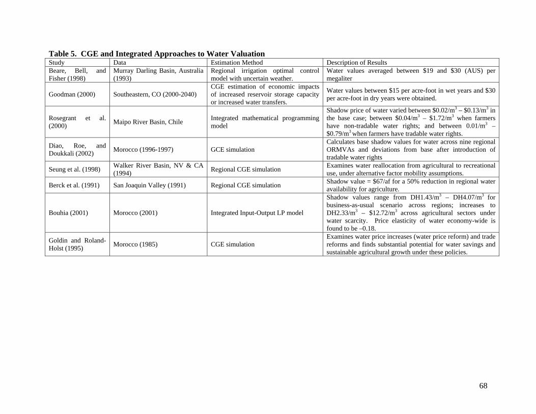
68

Table 5. CGE and Integrated Approaches to Water Valuation Study Data Estimation Method Description of Results Beare, Bell, and Fisher (1998)

Murray Darling Basin, Australia (1993)

Regional irrigation optimal control model with uncertain weather.

Water values averaged between $19 and $30 (AUS) per megaliter

Goodman (2000) Southeastern, CO (2000-2040) CGE estimation of economic impacts of increased reservoir storage capacity or increased water transfers.

Water values between $15 per acre-foot in wet years and $30 per acre-foot in dry years were obtained.

Rosegrant et al. (2000) Maipo River Basin, Chile Integrated mathematical programming

model

Shadow price of water varied between $0.02/m3 – $0.13/m3 in the base case; between $0.04/m3 – $1.72/m3 when farmers have non-tradable water rights; and between 0.01/m3 – $0.79/m3 when farmers have tradable water rights.

Diao, Roe, and Doukkali (2002) Morocco (1996-1997) GCE simulation

Calculates base shadow values for water across nine regional ORMVAs and deviations from base after introduction of tradable water rights

Seung et al. (1998) Walker River Basin, NV & CA (1994) Regional CGE simulation Examines water reallocation from agricultural to recreational

use, under alternative factor mobility assumptions.

Berck et al. (1991) San Joaquin Valley (1991) Regional CGE simulation Shadow value = $67/af for a 50% reduction in regional water availability for agriculture.

Bouhia (2001) Morocco (2001) Integrated Input-Output LP model

Shadow values range from DH1.43/m3 – DH4.07/m3 for business-as-usual scenario across regions; increases to DH2.33/m3 – $12.72/m3 across agricultural sectors under water scarcity. Price elasticity of water economy-wide is found to be –0.18.

Goldin and Roland-Holst (1995) Morocco (1985) CGE simulation

Examines water price increases (water price reform) and trade reforms and finds substantial potential for water savings and sustainable agricultural growth under these policies.