Michel Hénonand numerical experimentation on dynamical systems

Uriel FrischLaboratoire Joseph-Louis Lagrange

Observatoire de la Côte d’Azur, Nice

(with Yves Pomeau, LPS, ENS, Paris)

D.R. Marc Monticelli

Michel H�non Pionnier de l'exp�rimentation num�rique et astronome, Michel H�non est d�c�d� le 6 avril 2013 Nice dans sa 82e ann�e. Ancien �l ve de l'Ecole normale sup�rieure, il a commenc� sa carri re l'Institut d'Astrophysique, sous la direction d'Evry Schatzman, o� il a soutenu sa Th se d'Etat en 1961. En 1968 Il est parti l'Observatoire de Nice (devenu ult�rieurement Observatoire de la C�te d'Azur), dont la renaissance scientifique �tait anim�e par Jean-Claude Pecker. Michel H�non �tait avant tout un astronome, tr s connu pour ses travaux sur le probl me trois corps et sur les amas globulaires. ce sujet on consultera la notice biographique r�dig�e par Jacques Laskar ( para�tre). Paradoxalement, Michel H�non �tait encore plus connu mondialement chez tous ceux, physiciens ou math�maticiens Friday, November 29, 13

Hénon, Heiles and the KAM theory

•

•

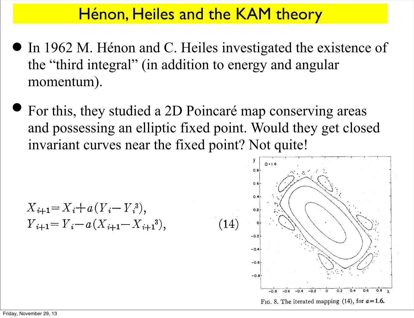
In 1962 M. Hénon and C. Heiles investigated the existence of the “third integral” (in addition to energy and angular momentum).

For this, they studied a 2D Poincaré map conserving areas and possessing an elliptic fixed point. Would they get closed invariant curves near the fixed point? Not quite!

1964AJ.....69...73H

1964AJ.....69...73H

78 M. HENON AND C. HEILES

far from the initial astronomical problem. Also, it is not obvious that an arbitrary area-preserving mapping corresponds to a possible dynamical situation. For these reasons, we give only a short account of the experiments made. The following mapping was studied:

Xi+l =Xi+a(Yi- Y i3), Y i+l = Yi-a(Xi+l-Xi+l3), (14)

where a is a constant. The coordinates of Pi are named here Xi and Vi.

. 698

.696

y

• 694

.692 • ".

... .. . ....

'" .

.... . .

." ... "' " ..

.. ·.424 -:422 -:420 -!418 -A16 -:414 -.412 -AIO -.408 -:406 -'04

X

FIG. 11. Enlargement of area D; Grid size = 0.0002.

Figure 8 shows the results for a= 1.6. Each set of points linked by a curve is the set of the successive transforms of an initial point Pl under the iterated mapping (14). The isolated points are also the successive transforms of a single initial point. The picture is quite similar to the right part of Fig. S. There is a central region occupied by a set of simple closed curves which surround the stable invariant point X = Y = 0; a chain of six islands (instead of five) ; and an outer "ergodic" region. Other chains of islands have been found here too. This similarity suggests that the problem of the area-preserving mapping is really identical with the dynam-ical problem of the third integral.

Up to 105 points have been computed for some of the curves, without any detectable deviation.

Figure 9 represents the upper half of Fig. 8, and Figs. 9-12 were produced in the following manner: initial points were chosen on a grid size indicated in the figure, throughout the whole area of the figure, and 1000 successive it era tions of each initial point were computed. Experience has shown that iterations of points which produce an "ergodic orbit" are eventually mapped to infinity; furthermore, this divergence is quite rapid, due to the cubic terms in (14). Thus in Fig. 9 for example, if all 1000 points remained in the vicinity of the origin (this being practically expressed by X2+ Y2< 100) the position of the initial point was marked with a dot;

otherwise, the position was left blank. The result is a replica of Fig. 8, the only difference being that Fig: 9 shows, to the scale of the grid, all initial points whose successive iterations lie on closed curves. Note that it is somewhat distorted, because the vertical and horizontal scales are not equal.

In order to investigate the mapping on a finer scale, we subdivide Fig. 9 into areas A, B, and C. Area A, ten times enlarged, is shown in Fig. 10. The most striking feature is the apparition of a multitude of small islands and tiny details, distributed in a random fashion. It can be remarked also that the boundary of the central region seems very sharp, whereas the boundary of the large island (on the left) is rather fuzzy. Area D of Fig . 10 was again enlarged ten times; see Fig. 11. Again a host of new details emerge. It seems very likely that this would go on indefinitely; with more magnification more details would appear, without end. These results sup-port the hypotheses made above, namely, that there is an infinite number of islands and that their set is dense everywhere .

Area B, which is farther from the center, is repre-sented on Fig. 12. The density of the islands is much smaller than in area A. Also a strong density gradient is apparent in the vertical direction. Area C, still farther out, was found to contain no dots at all to a grid size of 0.002 and therefore is not represented. Thus the density

.84r------------------,

.82

so .. y

.78

.76

.74LL-_<---->-_...w..--''--'''-'-_ ......... ---'L..--'-_-'---Ll -.46 -.44 -:42 -.40 -:38 -.36 .,34 .,32 ",28 "!.26

X

FIG. 12. Enlargement of area B; Grid size = 0.002.

of the islands seems to decrease very rapidly as the distance from the central region increases.

S. CONCLUSIONS

We return now to the original three-dimensional problem. The above experiments indicate that the behavior of the orbits is in general quite complicated, and there seems to be no hope of a simple general answer, such as: (a) the third isolating integral always exists; or (b) the third isolating integral does not exist.

© American Astronomical Society • Provided by the NASA Astrophysics Data System

Friday, November 29, 13

Lagrangian turbulence: the ABC flow

•

•364 Dombre, U . Frisch, J . M . Greene, M . Hinon, A. Mehr and A. M . Soward

FIGURE 5. A typical Poincak section, for the case A2 = 1 , B2 = 3% f? = S'

streamline, for which 5 x lo3 successive interactions have been computed. This indicates that the streamline itself wanders in a three-dimensional region of space, which i t fills more and more densely as time goes on.

In order to give a better idea of the three-dimensional structure of the flow, a number of Poincar6 sections will now be shown simultaneously. The standard arrangement is represented in figure 6. There are eight equidistant sections parallel to the (9, 2)-coordinate system, corresponding to x = 0, an, . . . , in, and similarly for the other directions - a total of 24 sections.

Figure 7 represents in this way a single chaotic streamline, starting from x = y = z = 0, again for the case A2 = 1, B2 = $, C2 = Q. A total of approximately lo5 points are represented.

The density of the points is not uniform; this is easily explained. Consider for instance a small region with area u in one of the surfaces of section y = const., and a small cylinder parallel to the local direction of flow, with base (T and height ydt. At the next intersection with the same surface of section, the image of this cylinder is another cylinder of base u' and height y' dt. Volumes in (2, y, Z) are preserved by the flow ; therefore mj dt = u'y' dt. Thus u varies as the inverse of y. It follows that the density of the points in a surface of section is proportional to y, the perpendicular component of velocity. In particular, the density falls to zero along the line defined by y = 0, or

B sinx+A cosz = 0.

.

(3-1) This line is the locus of the points where streamlines are tangential to the surface of section. The line (3.1), and the equivalent lines for the other directions of section, are represented on figure 8 for the same values of A, B, C as in figure 7.

The empty regions in figure 7 are the ordered regions. They can be seen to

354 T . Dombre, U . Frisch, J . M . Creene, M . Hinon, A. Mehr and A. M . Soward

particles following the streamlines may separate exponentially in time, while remaining in a bounded domain, and that individual streamlines may appear to fill entire regions of space (see also $3.1 ) . Thus the positions of fluid particles may become effectively unpredictable for long times. A class of flows with presumably chaotic streamlines has been identified by Arnold (1965). These flows involve three real parameters A, B and C; relative to rectangular Cartesian coordinates they are 2x-periodic in x, y, and z and have velocity u = (u, v, w), where

1 u = A sinz+Ccosy, v = Bsinx+Acosz, w = C sin y + B cosx.

Arnold (1965) was interested in three-dimensional steady-state solutions of the Euler equation

a,u+w x u = -vp*, (1.2)

where p. = p+;u2, w = v xu, v - u = 0. (1.3)

Streamlines lie on surfaces of constant p , and therefore can only be chaotic in regions where p. is constant, i.e. where the flow has the Beltrami properties:

0 = Au, u * V h = 0. (1.4a, b)

Since (1.4 b) implies that h is constant in chaotic regions, periodic solutions are sought with, for simplicity, h constant everywhere. Then the flow is a superposition of plane helical waves all having the same wavenumber Ihl and all the same (right or left) circular polarization. With 2x-periodicity in x, y, and z assumed, it follows that h2 = k2 + p 2 + q2, where k, p, and q are unsigned integers. Any integer n = ha which is not of the form 4a(8b+ 7) - with a and b natural integers - may be written as the sum of three integer squares (see for example Landau 1927, theorem 187). It is thus possible to set up a great variety of Beltrami flows, most of which presumably have chaotic streamlines. It is not our purpose to explore all these flows. We just point out that they may be of interest in so far as they provide a large class of possible topologies for steady, spatially periodic solutions of the Euler (or magnetostatic) equation without recourse to ‘non-analytic ’ solutions as in the work of Moffatt (1985) or Parker (1985). Henceforth we shall consider exclusively the simplest flows corresponding to Arnold’s choice of (1 .l) ; these have h2 = 1 and thus

(k, p, q ) = (1, 0,O) and permutations. (1.5) Early numerical experiments by HBnon (1966) have provided evidence for chaos in the special case A = 1/3, B = 1/2, C = 1. The special case A = B = C = 1 was introduced independently by Childress (1967, 1970) as a model for the kinematic dynamo effect. We propose to call these flows ABC (for Arnold, Beltrami, Childress). Another study of a flow with a chaotic Lagrangian structure has been made by Arter (1983). He uses the Boussinesq model, with a buoyancy term in the momentum equation which is not a gradient ; therefore the Beltrami property is not required for chaos.

From a fluid dynarnical viewpoint flows with chaotic streamlines are interesting because they may considerably enhance transport without being turbulent in the usual sense - they only display what might be called ‘Lagrangian turbulence’. Aref (1984) has shown that simple time-periodic two-dimensional flows can produce turbulent mixing of a passive scalar, limited only by the possible existence of Kolmogorov-Arnold-Moser (KAM) invariant surfaces. In three dimensions the same

The A(rnold)-B(eltrami)-C(hildress) flows are steady solutionsof the 3D incompressible Euler equations

In 1965 Arnold conjectured that ABC flows have chaotic streamlines and asked Hénon to check. This was done in 1966

Friday, November 29, 13

74 M. Henon

0 . 4

0 . 1

0 . 2

0 . 3

0 . 4

1.5 1.0 0 .5 0 0.5

Fig. 3. Same as Figure 2, but starting from xo = 0.63135448,

1.0 1.5

o= 0.18940634

These properties allow us to eliminate the "transient regime" in which thepoints approach the attractor, and which is not of much interest: we simply startfrom the close vicinity of the unstable point (12), by rounding off its coordinatesto 8 digits. This is done in F igure 3 and in the following figures. The points quicklymove away along the line of slope p2 since \λ2\ is appreciably larger than 1.

The attractor appears to consist of a number of more or less parallel "curves"the points tend to distribute themselves densely over these curves. The few gapsthat can still be seen on Figures 2 and 3 have probably no particular significance.Their locations are not the same on the two figures. They are simply due tostatistical fluctuations in the quasi random distribution of points, and they woulddisappear if more moints were plotted. Thus, the longitudinal structure of theattractor (along the curves) appears to be simple, each curve being essentially aone dimensional manifold.

The transversal structure (across the curves) appears to be entirely different,and much more complex. Already on Figures 2 and 3 a number of curves can beseen, and the visible thickness of some of them suggests that they have in fact anunderlying structure. F igure 4 is a magnified view of the small square of F igure 3:some of the previous "curves" are indeed resolved now into two or more com ponents. The number n of iterations has been increased to 105, in order to have asufficient number of points in the small region examined. The small square inFigure 4 is again magnified to produce F igure 5, with n increased to 106: again the

Strange Attractor 75

0.21

0.20

0 . 19

0.18

0 . 1 7 L

0,16

Q " 1 5 0.55 0.60 0.65 0.70

Fig. 4. Enlargement of the squared region of F igure 3. The number of computed points is increased

number of visible "curves" increases. One more enlargement results in Fig. 6,with n = 5 x 106: the points become sparse but new curves can still easily be traced.

These figures strongly suggest that the process of multiplication of "curves"will continue indefinitely, and that each apparent "curve" is in fact made of aninfinity of quasi parallel curves. Moreover, F igures 4 to 6 indicate the existenceof a hierarchical sequence of "levels", the structure being practically identicalat each level save for a scale factor. This is exactly the structure of a Cantor set.

The frames of F igures 4 to 6 have been chosen so as to contain the invariantpoint (12). This point appears to lie on the upper boundary of the attractor.Surprisingly, its presence is completely invisible on the figures; this contrasts withthe area preserving case, were stable and unstable invariant points play a veryconspicuous role (see for instance H enon, 1969). On the other hand, the presenceof the invariant point explains, locally at least, the hierarchy of similar structures:at each application of the mapping, the scale of the transversal structure ismultiplied by λx given by (13). At the same time, the points spread out along thecurves, as dictated by the value of λ2.

5. A Trapping Region

The fact that even after 5 x 106 iterations the points have not diverged to infinitysuggests that there is a region of the plane from which the points cannot escape.

76

0.191

0 . I9 0

0.189

0.188

0.187

0.186

°' 1 8 5 0.625 0.630 0.635

Fig. 5. Enlargement of the squared region of Figure 4; n = 106

M. Henon

"<;;: ΐ>.''

"' '** .' '''

I

,

1 Ί 1

0.640

This can be actually proved by finding a region R which is mapped inside itself.An example of such a region is the quadrilateral ABCD defined by

xA= 133, j ^ = 0.42, xB= 1.32, j / β = 0.133,

xc = 1.245, yc= 0A4, x ^ 1 . 0 6 , ^ = 0 . 5 . (14)The image of ABCD is a region bounded by four arcs of parabola, and it can beshown by elementary algebra that this image lies inside ABCD. Plotting thequadrilateral on Figure 2 or 3, one can verify that it encloses the observedattractor.

6. Conclusions

The simple mapping (4) appears to have the same basic properties as the Lorenzsystem. Its numerical exploration is much simpler: in fact most of the exploratorywork for the present paper was carried out with a programmable pocket computer(HP 65). For the more extensive computations of Figures 2 to 6, we used a IBM7040 computer, with 16 digit accuracy. The solutions can be followed over a muchlonger time than in the case of a system of differential equations. The accuracyis also increased since there are no integration errors.

Lorenz (1963) inferred the Cantor set structure of the attractor from reasoning,but could not observe it directly because the contracting ratio after one "circuit"

Hénon map as a model of the Lorenz-Pomeau attractor

30

I - INTRODUCTION

Lorenz I) proposed and studied a remarkable system of three coupled first-order

differential equations, representing a flow in three-dimensional space. The diver-

gence of the flow has a constant negative value, so that any volume shrinks exponen-

tially with time. Moreover, there exists a bounded region R into which every trajec-

tory becomes eventually trapped. Therefore, all trajectories tend to a set of mea-

sure zero, called attractor. In some cases the attractor is simply a point (which

is then a stable equilibrium point) or a closed curve (known as a limit cycle). But

in other cases the attractor has a much more complex structure. This is known as a

strange attractor. Inside the attractor, trajectories wander in an apparently erra-

tic manner. Moreover, they are highly sensitive to initial conditions.

All the known examples show that for differential systems of order 3

a "strange attractor" is an object which is intermediate "between" a surface

in the ordinary sense and a volume : it may be viewed as a surface with an infinite

number of sheets. As suggested by Thom 2) these strange attractors are continuous in

some dimensions and have the structure of a Cantor ensemble in the remaining dimen-

sion : consider a point ~ on the attractor, then a local system of curvilinear coor- ÷

dinates exists such as if x = (O,0,O) in this system, thus the point of coordinates

(ul,u2,u 3) is on the attractor when u I and u 2 vary in a finite interval around 0 and

when u 3 is an element of Cantor set (or "Cantor like" set). These strange attractors

have been already found in studying simple non linear differential equations related

to various problems : the case d = 3 has been already encountered in studies on the

unsteady Benard-Rayleigh thermo-convection ]) and on the reversals of the geomagnetic

field 3). As explained by Ruelle, the existence of strange attractors for so simple

deterministic systems clearly demonstrates the possibility of randomness in phenomena

as turbulence without any connection with the existence of an "infinite number of

degrees of freedom". We present here two cases of strange attractors that have been

found by studying the Lorenz system (section II) and then (section III) by trying to

reproduce the Poincar~ transform for this system by a planar quadratic transform.

II - THE STRANGE ATTRACTOR FOR THE LORENZ SYSTEM

II.A - The Lorenz system~transition from a strange attractor to a limit cycle

The Lorenz system is obtained by truncating the Oberbeck Boussinesq fluid equa-

tions for a layer heated from below. One keeps only a few spatial harmonics of the

velocity and temperature field at fixed wavenumber . The three remaining variables,

Xl,X 2 and x 3 are the amplitudes of the first spatial harmonics of the velocity and

temperature fluctuations and of the zeroth harmonic of the temperature fluctuation.

The time evolution of these three quantities is given by :

x I = o(x 2 - xl)

~2 = -XlX3 + rx] - x 2 (1)

x 3 = XlX 2 - Bx 3 ,

Lorenz(1963)

� = 10, � = 8/3

r = 28 I ZX

t X

JO~

OY

6t7

TWO STRANGE ATTRACTORS WITH A SIMPLE STRUCTURE

M. HENON+and Y. POMEAU ~

+Observatoire de Nice

~DPh-T CEN SACLAY BP n° 2 - 91190 Gif-sur-Yvette, France

ABSTRACT

Numerical computations have shown that, for a range of values of the parameters,

the Lorenz system of three non linear ordinary differential equations of first order

has a strange attractor whose structure may be understood quite easily.

We show that the same properties can be observed in a simple mapping of the 2

plane defined by : xi+ I = Yi + I - a x i , Yi+1 = b x i . Numerical experiments are

carried out for a = 1.4, b = 0.3. Depending on the initial point (Xo,Yo), the se-

quence of points obtained by iteration of the mapping either diverges to infinity

or tends to a strange attractor, which appears to be the product of a one-dimensional

manifold by a Cantor set. This strange attractor has basically the same structure

than a plane section of the attractor found for the Lorenz system.

Pomeau : r = 210

Henon: (x, y) 7! (y + 1� ax

2, bx)

72 M. H enon

thus reached by an entirely different road! The mapping (4), which was initiallyconstructed in empirical fashion, is in fact the most general quadratic mapping withconstant Jacobian.

One difference with the Lorenz problem is that the successive points obtainedby repeated application of T do not always converge towards an attractor;sometimes they "escape" to infinity. This is because the quadratic term in (4)dominates when the distance from the origin becomes large. However, for partic ular values of a and b it is still possible to prove the existence of a bounded "trappingregion" R, from which the points can never escape once they have entered it(see below Section 5).

T has two invariant points, given by

y = bx. (8)

These points are real for

(9)

When this is the case, one of the points is always linearly unstable, while the otheris unstable for

a>aί = 3(i b)2/ 4. (10)

3. Choice of Parameters

We select now particular values of a and b for a numerical study, b should besmall enough for the folding described by F igure 1 to occur really, yet not toosmall if one wishes to observe the fine structure of the attractor. The value b = 0.3was found to be adequate. A good value of a was found only after some experi menting. F or a<a0 or a>a3, where a0 is given by (9) and a3 is of the order of 1.55for i> = 0.3, the points always escape to infinity: apparently there exists no attractorin these cases. F or ao<a<a3, depending on the initial values (xo,yo\ either thepoints escape to infinity or they converge towards an attractor, which appears tobe unique for a given value of a. We concentrate now on this attractor. F orao<a<aί, where a1 is given by (10), the attractor is the stable invariant point.When a is increased over au at first the attractor is still simple and consists of aperiodic set of p points. (An equivalent attractor in the Lorenz problem wouldbe a limit cycle intersecting the surface of section p times). The value of p increasesthrough successive "bifurcations" as a increases, and appears to tend to infinityas a approaches a critical value α2, of the order of 1.06 for b = 0.3. F or a2<a<a3,the attractor is no more simple, and the behaviour of the points becomes erratic.This is the case in which we are interested. We adopt the following values:

0 = 1.4, b = 0.3. (11)

4. Numerical Results

Figure 2 shows the result of plotting 10000 successive points, obtained by iterationof T, starting from the arbitrarily chosen initial point xo = 0, yo = O; the verticalscale is enlarged to give a better picture. F igure 3 shows the result of 10000

Simple Chaos - The Hénon MapHénon's images are among the best known in twentieth century mathematics...

Amer. Math. Soc. Feature Column Oct. 2013 by Bill Casselman

Friday, November 29, 13

Optimisation: lattice gases, cosmological reconstruction

•(see also the lecture by Andrei Sobolevskii)

•

Optimal collision rules in 3D lattice gases (1988; with Rivet, Frisch and d’Humières)

Optimal reconstruction of the universe by Monge-Ampère-Kantorovich method (2003; with Brenier, Frisch, Loeper, Matarrese, Mohayaee and Sobolevskii)

Friday, November 29, 13

E

•

Friday, November 29, 13

E

•

Friday, November 29, 13