MINIMUM DISTANCE APPROACH TO INFERENCE WITH MANY INSTRUMENTS∗

Michal Kolesár†

Department of Economics and Woodrow Wilson School, Princeton University

This version 3.1.2, January 10, 2018

First circulated: November 2012.

Abstract

I analyze a linear instrumental variables model with a single endogenous regressorand many instruments. I use invariance arguments to construct a new minimum distanceobjective function. With respect to a particular weight matrix, the minimum distanceestimator is equivalent to the random effects estimator of Chamberlain and Imbens (2004),and the estimator of the coefficient on the endogenous regressor coincides with the limitedinformation maximum likelihood estimator. This weight matrix is inefficient unless theerrors are normal, and I construct a new, more efficient estimator based on the optimalweight matrix. Finally, I show that when the minimum distance objective function doesnot impose a proportionality restriction on the reduced-form coefficients, the resultingestimator corresponds to a version of the bias-corrected two-stage least squares estimator.I use the objective function to construct confidence intervals that remain valid when theproportionality restriction is violated.

Keywords: Instrumental Variables, Minimum Distance, Incidental Parameters, RandomEffects, Many Instruments, Misspecification, Limited Information Maximum Likelihood,Bias-Corrected Two-Stage Least Squares.JEL Codes: C13; C26; C36

∗Previously circulated under the title “Integrated Likelihood Approach to Inference with Many Instruments.” Iam deeply grateful to Guido Imbens and Gary Chamberlain for their guidance and encouragement. I also thankJoshua Angrist, Adam Guren, Whitney Newey, Jim Stock, Peter Phillips and participants at various seminars andconferences for their helpful comments and suggestions.†Correspondence to: Department of Economics, Julis Romo Rabinowitz Building, Princeton University, Princeton,

NJ 08544. Electronic correspondence: mkolesar@princeton.edu.

1

1 Introduction

This paper provides a principled and unified way of doing inference in a linear instrumental

variables model with a single endogenous regressor and homoscedastic errors in which

the number of instruments, kn, is potentially large. To capture this feature in asymptotic

approximations, I employ the many instrument asymptotics of Kunitomo (1980), Morimune

(1983), and Bekker (1994) that allow kn to increase in proportion with the sample size, n. I focus

on the case in which collectively the instruments have substantial predictive power, so that the

concentration parameter grows at the same rate as the sample size. I make no assumptions

about the strength of individual instruments. I allow the rate of growth of kn to be zero, in

which case the asymptotics reduce to the standard few strong instrument asymptotics.

The presence of many instruments creates an incidental parameters problem (Neyman and

Scott, 1948), as the number of first-stage coefficients, kn, increases with the sample size. To

directly address this problem, I use sufficiency and invariance arguments together with an

assumption that the reduced-form errors are normally distributed to reduce the data to a pair

of two-by-two matrices. In the absence of exogenous regressors, the first matrix can be written

as T =(y x

)′PZ(y x

)/n, where PZ is the projection matrix of the instruments Z, and y and x

are vectors corresponding to the outcome and the endogenous regressor. The second matrix,

S =(y x

)′(In − PZ)

(y x

)/(n− kn), where In is the identity, corresponds to an estimator of

the reduced-form covariance matrix. This solves the incidental parameters problem because the

distribution of T and S depends on a fixed number of parameters even as kn → ∞: it depends

on the first-stage coefficients only through the parameter λn, a measure of their collective

strength.

I then drop the normality assumption and use a restriction on the first moment of T implied

by the model to construct a minimum distance (md) objective function. This restriction follows

from the property of the instrumental variables model that the coefficients on the instruments

in the first-stage regression are proportional to the coefficients in the reduced-form outcome

regression. I use this md objective function to derive three main results.

First, I show that minimizing the md objective function with respect to the optimal weight

2

matrix yields a new estimator of β, the coefficient on the endogenous regressor, that exhausts

the information in T and S. In particular, this efficient md estimator is asymptotically more

efficient than the limited information maximum likelihood (liml) estimator when the reduced-

form errors are not normal. Standard errors can easily be constructed using the usual sandwich

formula for asymptotic variance of minimum distance estimators.1 The md approach thus

gives a simple practical solution to the many-instrument incidental parameters problem.

Second, I compare the md approach to that based on the invariant likelihood—the likelihood,

under normality, based on T and S. I show that, when combined with a particular prior on

λn, the likelihood is equivalent to the random-effects (re) quasi-maximum likelihood of

Chamberlain and Imbens (2004), and that maximizing it yields liml. Therefore, the random-

effects estimator of β is in fact equivalent to liml. Furthermore, I show that the re estimator of

the model parameters also minimizes the md objective function with respect to a particular

weight matrix. This weight matrix is efficient under normality, but not in general.

Third, I consider minimum distance estimation that leaves the first moment of T unrestricted.

This situation arises, for instance, when the instrumental variables model is used to estimate

potentially heterogeneous causal effects, as in Angrist and Imbens (1995). When the causal

effect is heterogeneous, the reduced-form coefficients are no longer proportional, so that the

first moment of T is unrestricted. In this case, the instrumental variables estimand β can be

interpreted as a weighted average of the marginal effect of the endogenous variable on the

outcome (Angrist, Graddy and Imbens, 2000). I show that the unrestricted minimum distance

estimator coincides with a version of the bias-corrected two-stage least squares estimator (Nagar,

1959; Donald and Newey, 2001), and use the md objective function to construct confidence

intervals that remain valid when the proportionality restriction is violated.

The md objective function is also helpful in deriving a specification test that is robust to

many instruments. By testing the restriction on the first moment of T, I derive a new test that is

similar to that of Cragg and Donald (1993), but with an adjusted critical value. The adjustment

ensures that the test is valid under few strong as well as many instrument asymptotics that also

allow for many regressors. In contrast, when the number of regressors is allowed to increase1Software implementing estimators and standard errors based on the md objective function is available at

https://github.com/kolesarm/ManyIV.

3

with the sample size, the size of the standard Sargan (1958) specification test converges to one,

as does the size of the test proposed by Anatolyev and Gospodinov (2011).

The paper draws on two separate strands of literature. First, the literature on many

instruments that builds on the work by Kunitomo (1980), Morimune (1983), Bekker (1994) and

Chao and Swanson (2005). Like Anatolyev (2013), I relax the assumption that the dimension of

regressors is fixed, and I allow them to grow with the sample size. Hahn (2002), Chamberlain

(2007), Chioda and Jansson (2009), and Moreira (2009) focus on optimal inference with many

instruments when the errors are normal and homoscedastic, and my optimality results build on

theirs. Papers by Hansen, Hausman and Newey (2008), Anderson, Kunitomo and Matsushita

(2010) and van Hasselt (2010) relax the normality assumption. Hausman, Newey, Woutersen,

Chao and Swanson (2012), Chao, Swanson, Hausman, Newey and Woutersen (2012), Chao,

Hausman, Newey, Swanson and Woutersen (2014) and Bekker and Crudu (2015) also allow for

heteroscedasticity. An interesting new development is to employ shrinkage or regularization to

solve the incidental parameters problem (see, for example, Belloni, Chen, Chernozhukov and

Hansen, 2012, Gautier and Tsybakov, 2014, or Carrasco, 2012). When combined with additional

assumptions on the model, these shrinkage estimators can be more efficient than the efficient

md estimator proposed here.

Second, the literature on incidental parameters dating back to Neyman and Scott (1948).

Lancaster (2000) and Arellano (2003) discuss the incidental parameters problem in a panel data

context. Chamberlain and Moreira (2009) relate invariance and random effects approaches

to the incidental parameters problem in a dynamic panel data model. My results on the

relationship between these two approaches in an instrumental variables model build on theirs.

Sims (2000) proposes a similar random-effects solution in a dynamic panel data model. Moreira

(2009) proposes to use invariance arguments to solve the incidental parameters problem.

The remainder of this paper is organized as follows. Section 2 sets up the instrumental

variables model, and reduces the data to the T and S statistics. Section 3 considers likelihood-

based approaches to inference under normality. Section 4 relaxes the normality assumption and

considers the md approach to inference. Section 5 considers md estimation without imposing

proportionality of the reduced-form coefficients. Section 6 studies tests of overidentifying

4

restrictions. Section 7 concludes. Proofs and derivations are collected in the appendix. The

supplemental appendix contains additional derivations.

2 Setup

In this section, I first introduce the model, notation, and the many instrument asymptotic

sequence that allows both the number of instruments and the number of exogenous regressors

to increase in proportion with the sample size. I then reduce the data to the low-dimensional

statistics T and S, and define the minimum distance objective function.

2.1 Model and Assumptions

There is a sample of individuals i = 1, . . . , n. For each individual, we observe a scalar outcome

yi, a scalar endogenous regressor xi, `n-dimensional vector of exogenous regressors wi, and

kn-dimensional vector of instruments z∗i . The instruments and exogenous regressors are treated

as non-random.

It will be convenient to define the model in terms of an orthogonalized version of the

original instruments. To describe the orthogonalization, let W denote the n× `n matrix of

regressors with ith row equal to w′i, and let Z∗ denote the n× kn matrix of instruments with

ith row equal to z∗i′. Let Z = Z∗ −W(W ′W)−1W ′Z∗ denote the residuals from regressing Z∗

onto W. Then the orthogonalized instruments Z ∈ Rn×kn are given by Z = ZR−1, where the

upper-triangular matrix R ∈ Rkn×kn is the Cholesky factor of Z′Z. Now, by construction, the

columns of Z are orthogonal to each other as well as to the columns of W.2

Denote the ith row of Z by z′i, and let Y ∈ Rn×2 with rows (yi, xi) pool all endogenous

variables in the model. The reduced form regression of Y onto Z and W can be written as

Y = Z(

π1,n π2,n

)+ W

(ψ1,n ψ2,n

)+ V, (1)

where V ∈ Rn×2 with rows v′i = (v1i, v2i) pools the reduced-form errors, which are assumed to

2This orthogonalization is sometimes called a standardizing transformation; see Phillips (1983) for discussion.

5

be mean zero and homoscedastic,

E[vi] = 0, and E[viv′i] = Ω. (2)

The reduced-form coefficients on the instruments are assumed to satisfy a proportionality

restriction, and the parameter of interest, β, corresponds to the constant of proportionality:

Assumption PR (Proportionality restriction). π1,n = π2,nβ.

The proportionality restriction implies that

yi = xiβ + w′i βwn + εi, (3)

where εi = v1i − v2iβ is known as the structural error, and βwn = ψ1,n − ψ2,nβ. This equation is

known as the structural equation. In Section 5, I allow for certain violations of this assumption,

such as when the effect of xi on yi is heterogeneous. Throughout the paper, I assume that

kn > 1, which implies that Assumption PR is testable; I discuss specification testing in Section 6.

In order to employ sufficiency and invariance arguments, I assume that vi has a normal

distribution:

Assumption N (Normality). The errors vi are i.i.d. and normally distributed.

This assumption has no effect on the consistency of estimators considered in this paper,

although it does affect their asymptotic distribution and asymptotic efficiency. I drop this

assumption in Sections 4 to 6 when I discuss a minimum-distance approach to inference.

To measure the strength of identification, I follow Chamberlain (2007) and Andrews,

Moreira and Stock (2008), and use the parameter

λn = π′2,nπ2,n · a′Ω−1a/n, a =

β

1

. (4)

The goal is to construct inference procedures that work well even if the number of instru-

ments kn and the number of exogenous regressors `n is large relative to sample size. I therefore

6

follow Anatolyev (2013) and Kolesár, Chetty, Friedman, Glaeser and Imbens (2015) and allow

both kn and `n to potentially grow with the sample size:

Assumption MI (Many instruments). (i) kn/n = αk + o(n−1/2) and `n/n = α` + o(n−1/2) for

some α`, αk ≥ 0 such that αk + α` < 1; (ii) The matrix(W Z

)is non-random and full column

rank kn + `n; (iii) ∑ni=1((z

′iπ2,n)4 + (z′iπ1,n)

4)/n2 = o(1); and (iv) λn = λ + o(1) for some λ > 0.

Assumption MI (i) weakens the many instrument sequence of Bekker (1994) by allowing `n to

grow with the sample size. The motivation for this is twofold. First, often the presence of many

instruments is the result of interacting a few basic instruments with many regressors (as in, for

example Angrist and Krueger, 1991), in which case both `n and kn are large. Second, oftentimes

the instruments are valid only conditional on a large set of regressors wi; for example, if the

instruments are randomly assigned within a school, we need to condition on school fixed

effects. By allowing αk = α` = 0, the assumption nests the standard few strong instrument

asymptotic sequence in which the number of instruments and regressors is fixed. Parts (ii)–(iv)

of Assumption MI are standard. Part (ii) is a normalization that requires excluding redundant

columns from W and excluding columns of Z that are redundant or already included in W. It

ensures that the reduced-form coefficients in (1) are well-defined. Part (iii) is used to verify the

Lindeberg condition. Part (iv) is the many-instruments equivalent of the relevance assumption.

It is equivalent to the assumption that the concentration parameter (Rothenberg, 1984), given

by π′2,nπ2,n/Ω22, grows at the same rate as the sample size.

2.2 Sufficient statistics and limited information likelihood

Under normality, the set of sufficient statistics is given by the least-squares estimators of the

reduced-form coefficients Πn =(π1,n π2,n

)and Ψn =

(ψ1,n ψ2,n

),

Π

Ψ

=

Z′Y

(W ′W)−1W ′Y

∈ R(kn+`n)×2,

7

and an unbiased estimator of the reduced-form covariance matrix Ω based on the residual sum

of squares,

S =1

n− kn − `nY′(In − ZZ′ −W ′(W ′W)−1W)Y ∈ R2×2, (5)

The advantage of working with the orthogonalized instruments is that now the rows of Π are

mutually independent. Since the distribution of Ψ is unrestricted, we can drop it from the

model and base inference on Π and S only as in Moreira (2003) and Chamberlain and Imbens

(2004). This step eliminates the potentially high-dimensional nuisance parameter Ψn, so that

the model parameters are now given by the triplet (β, π2,n, Ω).

Estimators considered in this paper will only depend on Π through the statistic

T =1n

Π′Π =1n

Y′ZZ′Y ∈ R2×2. (6)

Define the following functions of the statistics T and S:

QS (β, Ω) =b′Tbb′Ωb

, QT (β, Ω) =a′Ω−1TΩ−1a

a′Ω−1a, b =

1

−β

,

and let mmin and mmax denote the minimum and maximum eigenvalues of the matrix S−1T.

The likelihood of the model (1)–(2) under Assumptions PR and N is known as the limited

information likelihood (Anderson and Rubin, 1949). The limited information maximum

likelihood (liml) estimator of β is given by

βliml = argmaxβ

QT (β, S) = argminβ

QS (β, S) =T12 −mminS12

T22 −mminS22. (7)

It turns out that βliml is consistent and asymptotically normal under Assumption MI despite

the incidental parameters problem (Bekker, 1994). I will give some insight into this result in

Section 3.

Due to the incidental parameters problem, the (β, β) block of the inverse information matrix

of the limited information likelihood does not yield a consistent estimate of the asymptotic

variance of liml. The asymptotic distribution of βliml under Assumptions PR, N and MI is

8

given by (see Bekker, 1994 and Kolesár et al., 2015 for derivation)

√n(

βliml − β)⇒ N (0,Vliml,N) , (8)

where⇒ denotes convergence in distribution, and

Vliml,N =b′Ωb · a′Ω−1a

λ

(1 +

αk(1− α`)

1− αk − α`

1λ

). (9)

In contrast, the (β, β) block of the inverse information matrix is given by b′Ωb · a′Ω−1a/(nλn),

missing the correction factor in parentheses (see supplemental appendix for derivation). This

correction factor can be substantial even when the ratio of instruments to sample size, αk, is

small if λ is small.

2.3 Using invariance to reduce the dimension of the parameter space

To reduce the dimension of the parameter space, I follow Andrews, Moreira and Stock (2006),

Chamberlain (2007), Chioda and Jansson (2009), and Moreira (2009), and require decision

rules (procedures used for constructing point estimates and confidence intervals from the data)

to be invariant with respect to rotations of the instruments. In other words, changing the

co-ordinate system for the instruments should not affect inference about β—if we re-order

the instruments, or use a different orthogonalization procedure to construct Z, we should

get the same point estimate and confidence interval for β. A decision rule is invariant under

rotations of instruments if it remains unchanged under the transformation (Π, S) 7→ (gΠ, S),

where g ∈ O(kn), the group of kn × kn orthogonal matrices. A necessary and sufficient

condition for a decision rule to be invariant is that it depends on the data only through a

maximal invariant (Eaton, 1989, Theorem 2.3). A statistic m(Π, S) is maximal invariant if

(i) m(Π, S) = m(gΠ, S) for all g ∈ O(kn); and (ii) whenever m(Π, S) = m(Π, S) for some

Π, Π ∈ Rkn×2 and S, S ∈ R2×2, then (Π, S) = (gΠ, S) for some g ∈ O(kn). It is straightforward

to check that the pair of matrices (S, T) is a maximal invariant statistic. The distribution of

(S, T) depends on π2,n only through π′2,nπ2,n, or equivalently through λn = π′2,nπ2,n · a′Ω−1a/n.

9

This reduces the parameter space to (β, λn, Ω), which has a fixed dimension.3

There are two general approaches to constructing invariant decision rules based on the

maximal invariant (S, T). First, one can use the likelihood based on S and T, called the

invariant likelihood, Linv,n(β, λn, Ω; S, T). I consider this approach in detail in Section 3. The

disadvantage of this approach is that the validity of inference based on the invariant likelihood

is sensitive to Assumption N.

The second approach is to use moment restrictions on S and T implied by the model. In

particular, the reduced form (1)–(2) without any further assumptions implies

E[S] = Ω, (10a)

E[T − (kn/n)S] = Ξn, where Ξn =1n

(π1,n π2,n

)′ (π1,n π2,n

). (10b)

Under Assumption PR, the matrix of second moments of the reduced-form coefficients, Ξn, has

reduced rank,

Ξn = Ξ22,naa′ = Ξ22,n

β2 β

β 1

, (11)

with Ξ22,n = π′2,nπ2,n/n = λn/(a′Ω−1a). This rank restriction can be used to build a minimum

distance objective function4

Qn(β, Ξ22,n; Wn) = vech (T − (kn/n)S− Ξ22,naa′)′ Wn vech (T − (kn/n)S− Ξ22,naa′) , (12)

where Wn ∈ R3×3 is some weight matrix. Since the nuisance parameter Ω only appears in the

moment condition (10a), which is unrestricted, we can exclude the moment condition from

the objective function (12) without any loss of information (Chamberlain, 1982, Section 3.2). I

consider this approach in detail in Sections 4 to 6, where I show that this approach is more

attractive once Assumption N is relaxed.

3Similar arguments can be used to generalize the results in this paper to the case with more than one endogenousvariable. In particular, if dim(xi) = J and dim(Y) = n× (J + 1), then one can use invariance arguments to reducethe data to the same pair of matrices (S, T) defined in (5) and (6), now with dimension (J + 1)× (J + 1).

4The operator vech(A) transforms the lower-triangular part of A into a single column—when A is symmetric,as is the case here, the operator can be thought of as vectorizing A while removing the duplicates.

10

3 Likelihood-based estimation and inference

This section shows that by combining the invariant likelihood with a particular prior on

λn, we can construct a likelihood with a simple closed form that addresses the incidental

parameters problem. I show that this likelihood is equivalent to the random effects likelihood

of Chamberlain and Imbens (2004), and that maximizing it yields the liml estimator of β.

First consider maximizing the invariant likelihood. To state the result, let ωn = π2,n/‖π2,n‖,

so that Π and S can be parametrized by (β, ωn, λn, Ω). The parameter ωn lies on the unit

sphere Skn−1 in Rkn and it can be thought of as measuring the relative strength of the individual

instruments.

Lemma 1. The invariant likelihood Linv,n(β, λn, Ω; S, T) is maximized over β at βliml. This result also

holds if λn is fixed at an arbitrary value. Furthermore,

Linv,n(β, λn, Ω; S, T) =∫

Skn−1Lli,n(β, λn, ωn, Ω; Π, S)dFωn(ωn), (13)

where Lli,n denotes the limited information likelihood, and Fωn(·) denotes the uniform distribution on

the unit sphere Skn−1.

The first part of Lemma 1 generalizes the result in Moreira (2009) that the maximum invariant

likelihood estimator for β coincides with limlk when Ω is known. It also explains why the

limited information likelihood produces an estimator that is robust to many instruments, even

though the number of parameters in the likelihood increases with sample size: it is because

liml happens to coincide with the maximum invariant likelihood estimator.

The last part of Lemma 1 shows that the invariant likelihood is equivalent to the integrated

(marginal) likelihood that puts a uniform prior on ωn. This observation will allow me to

build the connection between the invariant likelihood and the random-effects likelihood of

Chamberlain and Imbens (2004). In particular, consider integrating the limited information

likelihood with respect to the following prior on λn, in addition to the uniform prior on ωn:

λn ∼λ

knχ2(kn). (14)

11

The hyperparameter λ corresponds to the limit of λn under Assumption MI. I allow it to be

determined by the data, so that the prior will be dominated in large samples. The two priors

on ωn and λn are equivalent to a single normal prior over the scaled first-stage coefficients

ηn = π2,n√

a′Ω−1a/n,

ηn ∼ N (0, λ/kn · Ikn). (15)

This prior is the random-effects prior proposed in Chamberlain and Imbens (2004). Therefore,

the integrated likelihood obtained after integrating the limited information likelihood over

the uniform prior on ωn and the chi-square prior on λn coincides with the re likelihood that

integrates the limited information likelihood over the normal prior (15). The re likelihood has

a simple closed form:5

Lre,n(β, λ, Ω) =∫

RknLli,n(β, ηn, ωn, Ω; Π, S)dFηn|λ(ηn | λ)

=∫

R

∫Skn−1Lli,n(β, λn, ωn, Ω; Π, S)dFωn(ωn)dFλn|λ(λn | λ)

= |S|n−kn−`n−3

2 ·(

1 +nkn

λ

)−kn/2

|Ω|−n−`n

2 e−12

(tr(Ω−1S)− nλQT (β,Ω)

kn/n+λ

),

(16)

where the last equality holds up to a normalizing constant, and S = (n − kn − `n)S + nT.

Chamberlain and Imbens (2004) motivate the re prior as a modeling tool: since the prior has

zero mean, it intuitively captures the idea that the individual instruments may not be very

relevant. This motivation leaves it unclear however, whether inference based on the re is

asymptotically valid when the first-stage parameters are viewed as fixed. The equivalence (16)

implies that one can indeed use the re likelihood for inference. In particular, since the invariant

likelihood has a fixed number of parameters and the invariant model is locally asymptotically

normal (Chioda and Jansson, 2009), inference based on it will be asymptotically valid by

standard arguments. Since the prior on λn gets dominated in large samples, this implies that

inference based on the re likelihood will also be asymptotically valid. Furthermore, since

by Lemma 1 constraining λn does not affect the maximum invariant likelihood estimator for β,

5Chamberlain and Imbens (2004) also consider putting a random effects prior only on some coefficients; thecoefficients on the remaining instruments are then assumed to be fixed. When referring to the random-effectslikelihood, I assume that we put a random-effects prior on all coefficients.

12

integrating the invariant likelihood with respect to the chi-square prior (14) will not affect it

either: it will still be given by βliml. The next proposition summarizes and formalizes these

results.

Proposition 1.

(i) The re likelihood (16) is maximized at

βre = βliml,

λre = maxmmax − kn/n, 0,

Ωre =n− kn − `n

n− `nS +

nn− `n

(T − λre

a′re

S−1 are

are a′re

), are =

(βre

1

).

(ii) If mmax > kn/n, the (1,1) element of the inverse Hessian of the re likelihood (16), evaluated at

(βre, λre, Ωre), is given by:

H11re

=b′

reΩrebre(λre + kn/n)

nλre

(QSΩre,22 − T22 +

c1− c

QSa′

reΩ−1

re are

)−1

,

where QS = QS (βre, Ωre), c = λreQS(kn/n+λre)(1−`n/n)

, and bre = (1,−βre)′.

(iii) Under Assumptions PR, N and MI, −nH11re

p→ Vliml,N , with Vliml,N given in Equation (9).

Part (i) of Proposition 1 formalizes the claim that the estimator of β remains unchanged under

the additional chi-square prior for λn. Part (ii) derives the expression for the inverse Hessian.

The condition mmax > kn/n makes sure that the constraint λ ≥ 0 does not bind, otherwise

the Hessian is singular. It holds with probability approaching one under Assumption MI (iv),

as mmax − kn/np→ λ > 0. Part (iii) proves that the extra prior on λn gets dominated in

large samples so that the inverse Hessian can be used to estimate the asymptotic variance

of βliml (one could also use the inverse Hessian of the invariant likelihood, although this

involves numerical optimization since maximum invariant likelihood estimates of λn and Ω

are not available in closed form). It is important that the prior on λn is chosen such that the

prior is dominated in large samples. For example, Lancaster (2002) suggests integrating the

orthogonalized incidental parameters out with respect to a uniform prior. Here such prior

13

corresponds to a flat prior on ηn, which is equivalent to a uniform prior on ωn, and an improper

prior on λn, obtained by taking the limit of (14) as λ→ ∞. However, this improper prior on

λn will never get dominated by the data, and as a result, it can be shown that the resulting

likelihood will fail to produce valid confidence intervals.

4 Minimum distance estimation and inference

In this section, I first show that the random effects estimator is in fact equivalent to a minimum

distance estimator that uses a particular weight matrix. This weight matrix weights the

restrictions efficiently under normality, but not otherwise. I derive a new estimator of β based

on the efficient weight matrix that is more efficient than liml when the normality assumption

is dropped. Moreover, unlike inference based on the random effects likelihood, minimum-

distance-based inference will be asymptotically valid even if the reduced-form errors are not

normally distributed.

To simplify the expressions in this section, let Dd ∈ Rd2×d(d+1)/2, Ld ∈ Rd(d+1)/2×d2, and

Nd ∈ Rd2×d2denote the duplication matrix, the elimination matrix, and the symmetrizer matrix,

respectively (see Magnus and Neudecker (1980) for definitions of these matrices). The sym-

metrizer matrix has the property that for any d× d matrix A, Nd vec(A) = (1/2) vec(A + A′).

The duplication matrix transforms the vech operator into a vec operator, and the elimi-

nation operator performs the reverse operation, so that for a symmetric d × d matrix A,

Dd vech(A) = vec(A), and Ld vec(A) = vech(A).

4.1 Random effects and minimum distance

The random effects likelihood (16) and the minimum distance objective function (12) both

leverage the rank restriction (11) to construct an estimator of β. There should therefore exist a

weight matrix such that the random effects estimator of (β, Ξ22,n) is asymptotically equivalent

to a minimum distance estimator with respect to this weight matrix. The next proposition

shows that if the weight matrix is appropriately chosen, the minimum distance and random

effects estimators are in fact identical.

14

Proposition 2. Consider the minimum distance objective function (12) with respect to the weight matrix

Wre = D′2(S−1 ⊗ S−1)D2. (i) The objective function is minimized at (βre, Ξ22,re), where Ξ22,re =

λre/(a′re

Ω−1re

are) (ii) Under Assumptions PR, N and MI, the weight matrix Wre is asymptotically

optimal.

The second part of Proposition 2 shows that if the errors are normally distributed, then the

random effects weight matrix Wre weights the moment condition (10b) efficiently under many-

instrument asymptotics, even though Wre doesn’t converge to the inverse of the asymptotic

variance of the moment condition. The proof shows that the inverse of the asymptotic variance

is not the unique optimal weight matrix, but that there exists a whole class of optimal weight

matrices, and that this class includes Wre.6 As I show in the next subsection, this optimality

result is sensitive to Assumption N.

The equivalence between minimum distance and re estimators is related to the observation

in Bekker (1994) that liml can be thought of as a method-of-moments estimator in the sense

that it satisfies (T −mminS)(1,−βliml)′ = 0, which is similar to a first-order condition of the

objective function (12) when the weight Wre is used. It is also related to Goldberger and Olkin

(1971), who consider a minimum distance objective function based on the proportionality

restriction PR,

Qgo,n(β, π2,n) = vec(Π− π2,na′

)′ (S−1 ⊗ Ikn

)vec

(Π− π2,na′

). (17)

Goldberger and Olkin (1971) show that this objective function is minimized at βliml. However,

the number of parameters in this objective function diverges to infinity under Assumption MI,

so it cannot be used for inference.

4.2 Minimum distance estimation under non-normal errors

The efficiency of βliml as well as the expression for the asymptotic distribution of βliml given

in (9) depend on Assumption N. This sensitivity to the normality assumption is similar to

6The standard condition that the weight matrix converges to the inverse of the asymptotic covariance matrixof the moment conditions is sufficient, but not necessary for asymptotic efficiency (Newey and McFadden, 1994,Section 5.2).

15

the efficiency results for the maximum likelihood estimator in panel-data models in which

identification is based on covariance restrictions (Arellano, 2003, Chapter 5.4).

In order to derive the optimal weight matrix as well as the correct asymptotic variance

formulae under non-normality, we first need the limiting distribution of the moment condi-

tion (10b). The moment condition depends on the data through the three-dimensional statistic

vech(T− (kn/n)S). It can be seen from the definition of T and S given in Equations (5) and (6)

that this statistic can be written as a quadratic form

T − kn

nS =

1n

Y′HY =1n(Zπ2,na′ + V)′H(Zπ2,na′ + V),

where

H = ZZ′ − kn

n− kn − `n(In −W(W ′W)−1W ′ − ZZ′).

We need to impose some regularity conditions on the components of the quadratic form.

Let diag(A) denote the n-vector consisting of diagonal elements of an n-by-n matrix A, and let

δn = diag(H)′ diag(H)/kn.

Assumption RC (Regularity conditions). (i) The errors vi are i.i.d, with finite 8th moments; (ii) For

some δ, µ ∈ R, as n→ ∞, δn → δ, and π′2,nZ′ diag(H)/√

nkn → µ

Part (i) relaxes the normality assumption on the errors. Part (ii) ensures the asymptotic

covariance matrix is well-defined.

Lemma 2. Under Assumptions PR, MI and RC:

(i)√

n vech(T − (kn/n)S− Ξ22,naa′)⇒ N (0, ∆), with ∆ = L2(∆1 + ∆2 + ∆3 + ∆′3)L′2, where

∆1 = 2N2(Ξ22aa′ ⊗Ω + Ω⊗ Ξ22aa′ + τΩ⊗Ω,

), τ = αk(1− α`)/(1− αk − α`),

∆2 = αkδ[Ψ4 − vec(Ω) vec(Ω)′ − 2N2(Ω⊗Ω)

], Ψ4 = E[(viv′i)⊗ (viv′i)],

∆3 = 2N2(√

αkµΨ′3 ⊗ a), Ψ3 = E[(viv′i)⊗ vi],

and Ξ22 = λ/(a′Ω−1a).

(ii) Let M = In − ZZ′ −W(W ′W)−1W ′, let V = MY with rows v′i denote estimates of the reduced

16

form errors, and let π2 denote the second column of Π. Then

Ψ3 =∑i[(viv′i)⊗ vi]

∑i,j M3ij

p→ Ψ3,

Ψ4 =∑i(viv′i)⊗ (viv′i)−

[∑i M2

ii −∑i,j M4ij

](2N2Ω⊗ Ω + vec(Ω) vec(Ω)′)

∑i,j M4ij

p→ Ψ4,

and µ = π2Z′ diag(H)/√

nknp→ µ.

Part (i) shows that the asymptotic variance consists of three distinct terms. If the errors are

normally distributed, then ∆2 = ∆3 = 0. The term ∆2 accounts for excess kurtosis of the errors,

and the term ∆3 accounts for skewness. Part (ii) provides consistent estimators for the third

and fourth moments of the errors, and for µ. Since the probability limits of S and T do not

depend on Assumption N, the other components of ∆1, ∆2 and ∆3 can be consistently estimated

by βre, Ωre, and Ξ22,re = λre/(a′re

Ω−1re

are). Therefore, a consistent estimator of the asymptotic

covariance matrix ∆ is given by

∆ = L2(∆1 + ∆2 + ∆3 + ∆′3)L′2, (18)

where the terms ∆1, ∆2, and ∆3 are given by replacing β, Ξ22, and Ω in the definitions of ∆1, ∆2,

and ∆3 by their random-effects estimators, replacing Ψ3 and Ψ4 by Ψ3 and Ψ4, and replacing δ

and µ by δn and µ.

Inference based on LIML Since βliml is a minimum distance estimator, its asymptotic vari-

ance is given by the (1,1) element of the matrix

(G′WG)−1G′W∆WG(G′WG)−1, (19)

where W = D′2(Ω−1 ⊗ Ω−1)D2 = plim Wre, and G is the derivative of the moment condi-

tion (10b),

G = L2

(Ξ22

(a⊗

(10

)+(

10

)⊗ a)

a⊗ a

).

17

This element evaluates as

Vliml = Vliml,N +2√

αkµ

Ξ222

E[(v2i − γεi)ε2i ] +

αkδ

Ξ222

E[ε2i (v2i − γεi)

2 − |Ω|],

where εi = v1i − v2iβ is the structural error, and γ is regression coefficient from projecting v2i

onto it,

γ = (Ω12 −Ω22β)/(b′Ωb), (20)

The term Vliml,N (given in Equation (9)) corresponds to the asymptotic variance of βliml under

normal errors. The two remaining terms are corrections for skewness and excess kurtosis.

Anatolyev (2013) derives the same asymptotic variance expression by working with the explicit

definition of βliml. If α` = 0, then Vliml reduces to the asymptotic variance given in Hansen

et al. (2008), Anderson et al. (2010), and van Hasselt (2010). Due to the presence of the two

extra terms, the inverse Hessian will no longer estimate the asymptotic variance consistently.

However, a consistent plug-in estimator of (19) can easily be computed by replacing ∆ by ∆

and replacing a, Ξ22, and Ω in the expressions for G and W by are, Ξ22,re and Ωre.

Efficient minimum distance estimator Using the inverse of the variance estimator (18) as a

weight matrix in the minimum distance objective function yields an efficient minimum distance

(emd) estimator

(βemd, Ξ22,emd) = argminβ,Ξ22

Qn(β, Ξ22,n; ∆−1).

Since the objective function is a fourth-order polynomial in two arguments, the solution can be

easily found numerically. It then follows by standard arguments (see, for example, Newey and

McFadden (1994)), that when αk > 0,

√n(βemd − β)⇒ N (0,Vemd),

where Vemd corresponds to (1,1) element of the matrix (G′∆−1G)−1, which evaluates as

Vemd = Vliml −1

Ξ222(b′Ωb)2

(√αkµE[ε3

i ] + αkδE[(v2i − γεi)ε3i ])2

2τ + αkδκ, (21)

18

where

κ = E[ε4i /(b′Ωb)2 − 3] (22)

measures excess kurtosis of εi. A consistent plug-in estimator of Vemd can be easily constructed

by replacing ∆ by ∆, and replacing Ξ22 and β in the expression for G by their random-effects,

or emd estimators.

There is a slightly stronger sense in which βemd is efficient than just being efficient in

the class of minimum distance estimators: it exhausts the information available in (S, T). In

particular, as argued in van der Ploeg and Bekker (1995), the efficiency bound for estimators

that are smooth functions of (S, T) is given by the efficient minimum distance estimator based

on the moment conditions (10a) and (10b). However, since the nuisance parameter Ω only

appears in the first moment condition (10a), which is unrestricted, we can exclude it from the

objective function, and the minimum distance estimator of β with respect to an efficient weight

matrix will achieve the same asymptotic variance (Chamberlain, 1982, Section 3.2).

Hahn (2002) shows that when the errors are restricted to be normal, an estimator that

exhausts the information in (S, T) will have variance given by Vliml. Anderson et al. (2010)

generalize this result by allowing the errors to belong to the family of elliptically contoured

distributions.7 Equation (21) shows that this is not true in general. Indeed, the Anderson et al.

(2010) result obtains as a special case, since for elliptically contoured distributions, Ψ3 = 0, so

that E[ε3i ] = 0 and Ψ4 is proportional to vec(Ω) vec(Ω)′ + 2N2Ω⊗Ω (Wong and Wang, 1992),

which implies E[(v2i − γεi)ε3i ] = 0, so that the second term in (21)—the efficiency gain over

liml—equals zero.

The other special case in which the efficiency gain is zero is when δ = 0, which by the

Cauchy-Schwarz inequality, µ2 ≤ δΞ22, implies µ = 0. The term δ measures the balance of

the design matrices Z and W. If the diagonal elements of the projection matrices (ZZ′)ii

and (W(W ′W)−1W)ii, called the leverage of i, are constant across i, then δn = 0, and δn, and

hence δ, generally increases with the variability of the leverages. Suppose, for instance, that

7A mean-zero random vector has an elliptically contoured distribution if its characteristic function can bewritten as ϕ(t′V t), for some matrix V and some function ϕ. The multivariate normal distribution is a special case,with ϕ(t) = e−t′t/2.

19

each observation i belongs to one of kn + 1 groups, numbered 0, . . . , kn, and that there are nj

observations in group j. Let the kn-vector of instruments z∗i correspond to a vector of group

indicators, with group 0 excluded, and suppose that the only covariate is an intercept.8 Then,

(W(W ′W)−1W ′)ii = 1/n, and (ZZ′)ii = 1/nj(i) − 1/n, where j(i) denotes the group that i

belongs to (see supplemental appendix for derivation). It then follows from the definition of δn

that δn = 0 if and only if all groups have equal size, and that the magnitude of δn increases

with ∑knj=0 1/nj, which can be thought of as a measure of group size variability.

Recently, Cattaneo, Crump and Jansson (2012), in the context of few strong instrument

asymptotics, proposed a modification of liml that is more efficient than liml when the

distribution of the reduced-form errors is not normal. The modification was to use a more

efficient estimator of the reduced-form coefficients Πn than Π. Cattaneo et al. (2012) use a

two-step estimator that uses a kernel estimator of the distribution of the reduced-form errors

in the first step Under Assumption MI, when the number of regressors in the reduced-form

regression increases with sample size however, this kernel estimator will not be consistent, and

so this estimator is unlikely to perform well in settings with many instruments. In contrast,

βemd uses the same estimator Π of Πn as liml, but combines the information about β in Π

in a more efficient way. On the other hand, βemd requires αk > 0 for the efficiency gain to be

non-zero.

5 Minimum distance estimation without rank restriction

Assumption PR implies that the matrix Ξn is reduced rank. In particular, it implies that there

are two sources of information for estimating β,

Ξ11,n = Ξ12,nβ, and (23)

Ξ12,n = Ξ22,nβ. (24)

8This setup arises when individuals are randomly assigned to groups. For example, if a defendant is randomlyassigned to one of kn + 1 judges who differ in their sentencing severity, then one can use judge indicators asinstruments for the length of sentence of the defendant, as in Aizer and Doyle (2015) or Dobbie and Song (2015).

20

The minimum distance objective function (12) weights both sources of identification. In

this section, I consider estimation without imposing the rank restriction that Ξ11,n/Ξ12,n =

Ξ12,n/Ξ22,n. I show that a version of the bias-corrected two-stage least squares estimator (Nagar,

1959; Donald and Newey, 2001) is equivalent to a minimum distance estimator that only

uses (24) to estimate β, and derive standard errors that remain valid when (23) does not hold.

5.1 Motivation for relaxing the rank restriction

There are two important cases in which the ratios Ξ12,n/Ξ22,n and Ξ11,n/Ξ12,n, which correspond

to estimands of the reverse two-stage least squares and two-stage least squares estimators under

standard asymptotics (Kolesár, 2013), are not necessarily equal to each other, but Ξ12,n/Ξ22,n, is

still of interest.

The first case arises when the effect of xi on yi is heterogeneous, as in Imbens and Angrist

(1994). Let yi(x) denote the potential outcome of individual i when assigned xi = x, and

similarly let xi(z) denote the potential value of the endogenous variable if the individual was

assigned zi = z. We observe yi = yi(xi) and xi = xi(zi). For simplicity, suppose there are

no regressors wi beyond a constant. Suppose that (i) zi affects the outcome only through

its effect on xi: yi(x)x∈X is independent of zi, where X denotes the support of xi; and

(ii) Monotonicity holds: for any pair (z1, z2), P(xi(z1) ≥ xi(z2)) equals either zero or one.

Then Ξ12,n/Ξ22,n can be written as a particular weighted average of average partial derivatives

β(z) = E[∂yi(xi(z))/∂x] (see Angrist and Imbens (1995) and Angrist et al. (2000) for details).

However, unless β(z) is constant, the rank restriction will not hold, and the ratio Ξ11,n/Ξ12,n

may be outside of the convex hull of the average partial derivatives (Kolesár, 2013), which

makes it hard to interpret.

The second case arises when instruments have a direct effect on the outcome. In this case, the

coefficient π1,n in the reduced-form regression of the outcome on instruments is given by π1,n =

π2,nβ + βzn, where βz

n measures the strength of the direct effect. The structural equation (3) no

longer holds—instead we have yi = xiβ + w′i βwn + z′iβ

zn + εi. Without any restrictions on βz

n, the

parameter β is no longer identified. However, Kolesár et al. (2015) show that if the direct effects

are orthogonal to the effects of the instruments on the endogenous variable in the sense that

21

π′2,nβzn/n → 0 as n → ∞, then β can still be consistently estimated. In particular, under this

condition Ξ12,n/Ξ22,n = β + βzn′π2,n/π′2,nπ2,n → β. In contrast, Ξ11,n/Ξ12,n → β only if direct

effects disappear asymptotically so that βzn′βz

n/n→ 0.

5.2 Unrestricted minimum distance estimation

To relax the rank restriction on Ξn, define βn simply as the ratio Ξ12,n/Ξ22,n, and consider the

objective function

Qumd

n (β, Ξ11, Ξ22; Wn) =

vech(

T − (kn/n)S−(

Ξ11 Ξ22βΞ22β Ξ22

))′Wn vech

(T − (kn/n)S−

(Ξ11 Ξ22β

Ξ22β Ξ22

)), (25)

where Wn ∈ R3×3 is some weight matrix. If we restrict Ξ11,n to equal to Ξ22,nβ2n, then minimizing

this objective function is equivalent to minimizing the original objective function (12). If Ξ11,n

is unrestricted, the weight matrix does not matter since then the model is exactly identified.

The unrestricted minimum distance estimators will be given by their sample counterparts,

Ξ22,umd = T22 − (kn/n)S22, Ξ11,umd = T11 − (kn/n)S11,

and

βumd =T12 − (kn/n)S12

T22 − (kn/n)S22.

The unrestricted minimum distance estimator for βn coincides with the modified bias-corrected

two-stage least squares estimator (Kolesár et al., 2015), a version of the bias-corrected two-stage

least squares estimator. The version proposed by Donald and Newey (2001) multiplies S12 and

S22 by kn−2n

n−kn−`nn−kn+2 instead of kn/n. The motivation for the version in Kolesár et al. (2015) was

to modify the Donald and Newey estimator to make it consistent when α` > 0. However, it can

also be viewed as a minimum distance estimator that puts no restrictions on the reduced form.

The next proposition derives its large-sample properties.

Proposition 3. Suppose that Assumption MI(i)–(iii) and Assumption RC hold, Ξn = Ξ + o(1) where

Ξ is a positive semi-definite matrix with Ξ22 > 0, and that (π1,n − π2,nβn)′Z′ diag(H)/√

nkn =

22

µ + o(1) for some µ. Then√

n(

βumd − βn)⇒ N (0, Vumd),

where,

Vumd = Vemd + V∆ +|Ξ|Ω22/Ξ22 + 2

√αkµE[v2

2iεi]

Ξ222

V∆ =

((2τ + αkδκ)γ(b′Ωb)2 +

√αkµE[ε3

i ] + αkδE[ε3i (v2i − γεi)]

)2

(b′Ωb)2(2τ + αkδκ)Ξ222

where κ, γ are defined as in (20) and (22), with β = Ξ12/Ξ22, and εi = v2i − v1iβ.

The asymptotic variance Vumd corresponds to the (1,1) element of the matrix G−1umd

∆umdG−1umd

′,

where Gumd is the derivative of the moment condition,

Gumd =

1 1 0

Ξ22 0 β

0 0 1

, so that G−1umd

′ ( 100

)=

1Ξ22

(0, 1,−β),

and, as shown in the proof, ∆umd = L2(∆1,umd + ∆2 + ∆3,umd + ∆′3,umd)L′2 is the asymptotic

variance of the moment condition (10b), with

∆1,umd = 2N2(Ξ⊗Ω + Ω⊗ Ξ + τΩ⊗Ω), ∆3,umd = 2√

αkN2

Ψ′3 ⊗

µ + µβ

µ

,

and ∆2 given in Lemma 2. If Ξ = Ξ22aa′, then the expressions for ∆1,umd and ∆3,umd reduce to

those for ∆1 and ∆3 given in Lemma 2.

The asymptotic variance consists of three components. The first term coincides with the

asymptotic variance of emd given in Equation (21). The second component, V∆, represents the

asymptotic efficiency loss relative to βemd when the rank restriction holds; it quantifies the

price for not using information contained in (23) when the rank restriction holds. Unlike the

efficiency loss of liml, the term is positive even when the errors are normal, in which case

it simplifies to 2τ(Ω12 −Ω22β)2/Ξ222, which is only zero if there is no endogeneity (that is,

E[xiεi] = 0). Finally, the last component represents the increase in asymptotic variance due to

23

the failure of rank restriction; when PR holds, |Ξ| = 0 and µ = 0, and this term drops out.

The asymptotic variance can be easily consistently estimated by

Vumd =1

Ξ222,umd

(0, 1,−βumd)′∆umd(0, 1,−βumd),

where ∆umd is a plug-in estimator based on Ξumd = T − kn/nS, βumd, Ω = S, and estimators

of Ψ3 and Ψ4 given in Lemma 2. Confidence intervals based on βumd and Vumd will then be

robust to both many instruments, and failure of the proportionality restriction (1).

It is possible to reduce the asymptotic mean-squared error of the minimum distance

estimator by minimizing the minimum distance objective function subject to the constraint that

Ξn be positive semi-definite (which has to be the case since Ξn is a matrix of second moments of

π2,n and π1,n), which is equivalent to the constraint Ξ11,n ≥ β2nΞ22,n. If the weight matrix Wn is

used, then the resulting estimator will be a mixture between βumd, and the restricted minimum

distance estimator that minimizes (12) with respect to Wn: when T − (kn/n)S is positive

semi-definite, then the estimator equals βumd; otherwise, the minimum distance objective is

minimized at a boundary, and the estimator equals the restricted minimum distance estimator.

When Ξn is full rank, then the constraint won’t bind in large samples, and the estimator will

be asymptotically equivalent to βumd. However, when Ξn is reduced-rank, the mixing will

deliver a smaller asymptotic mean-squared error. The disadvantage is that the estimator will be

asymptotically biased, which makes inference more complicated. See supplemental appendix

for details.

6 Tests of overidentifying restrictions

The proportionality restriction PR is testable. In this section, I discuss a simple test based

on the minimum distance objective function, and compare it to some alternatives previously

proposed in the literature.

In the invariant model, testing Assumption PR is equivalent to testing the null that Ξn is

reduced-rank against the alternative that it is positive definite. A simple way to implement the

test is to compare the value of the minimum distance objective function (25) minimized subject

24

to the restriction that |Ξn| is reduced rank with its value when it is minimized subject to |Ξn|

being positive semi-definite. When Wre is used as a weight matrix, the test statistic is given by

(see supplemental appendix for derivation)

Jmd = minΞ11=Ξ22β2

Qumd

n (β, Ξ11, Ξ22; Wre)− minΞ11≥Ξ22β2

Qumd

n (β, Ξ11, Ξ22; Wre)

=

0 if mmin ≤ kn/n,

(mmin − kn/n)2 otherwise.

The test statistic depends on the data through the minimum eigenvalue of S−1T. Because the

weight matrix Wre is not optimal, the large-sample distribution of Jmd is not pivotal under the

null: if kn → ∞ as n → ∞, then in large samples, n2 Jmd/kn will be distributed as a mixture

between a χ21 distribution scaled by 2(1−α`)

1−αk−α`+ δκ (with κ defined in Equation (22)), and a

degenerate distribution with a point mass at 0. One solution would be to divide the test

statistic by 2(1−α`)1−αk−α`

+ δκ and use a critical value based on the 90% quantile of a χ21 distribution,

or, equivalently, reject whenever (n/√

kn)(mmin − kn/n)/√

2(1−α`)1−αk−α`

+ δκ is greater the 95%

quantile of a standard normal distribution. However, since the asymptotic distribution changes

when kn is fixed, this won’t yield valid inference when kn is fixed. Using arguments similar to

Anatolyev and Gospodinov (2011), the next proposition proposes a modification that ensures

size control whether kn is fixed or grows with the sample size.

Proposition 4. Suppose Assumptions PR, MI and RC hold. Suppose also that if kn = K is fixed, then

supn≥1 maxi=1,...,n(ZZ′)2ii = o(1). Then:

(i) If kn → ∞, n√kn(mmin− kn/n)⇒ N (0, 2(1−α`)

1−αk−α`+ δκ). If kn = K is fixed, then nmmin ⇒ χ2

K−1.

(ii) Let δn = diag(H)′ diag(H)/kn, let κ = (bre ⊗ bre)′Ψ4(bre ⊗ bre)/(b′reSbre)2 − 3, and let Φ

denote cdf of a standard normal distribution. The test that rejects whenever nmmin is greater than

the

1−Φ(√

(n−kn)n−kn−`n

+ δn κ2 ·Φ−1(ns)

)quantile of the χ2

kn−1 distribution has asymptotic size equal to ns. This holds whether kn = K is

fixed or kn → ∞.

25

When kn → ∞, the test is asymptotically equivalent to the test proposed in the previous

paragraph. However, unlike that test, it also remains valid under the few strong instrument

asymptotics with kn fixed. In this case, it is asymptotically equivalent to the Cragg and

Donald (1993) test, which is based on the minimum distance objective function (17), and rejects

whenever nmmin is greater than the 1− ns quantile of χ2kn

distribution. The test can therefore

be interpreted as a Cragg-Donald test with a modified critical value that ensures size control

under few strong, as well as many-instrument asymptotics.

It is interesting to compare this test to some other tests proposed in the literature. In the

context of few strong instrument asymptotics, the most popular test is due to Sargan (1958).

The test statistic can be written as Js = mmin1−kn/n−`n/n+mmin

, and the critical value is given by

1− ns quantile of χ2kn

. Anatolyev and Gospodinov (2011) show that if αk > 0 and α` = 0 and

the errors are normal, the Sargan test is mildly conservative. With αk = 0.1 for example, the

asymptotic size of the test with nominal size 0.05 is given by 0.04. Anatolyev and Gospodinov

(2011) therefore propose an adjustment to the critical value similar to the one proposed here to

match the asymptotic size with the nominal size. Unfortunately, this solution is not robust to

allowing the number of exogenous regressors to increase with the sample size: if α` > 0, the

asymptotic size of the Sargan test converges to one (see supplemental appendix for details).

Lee and Okui (2012) propose a different modification of the Sargan test that controls size under

conditions similar to Proposition 4, provided that, in addition, α` = 0 and kn → ∞. In contrast,

the test proposed here will work irrespective of the number of regressors or instruments; the

researcher doesn’t have to determine what type of asymptotics are appropriate.

Another alternative to the test in Proposition 4 would be to use the efficient weight matrix

instead of Wre in the minimum distance objective function. Such a test would in general direct

local asymptotic power to different alternatives, and, without specifying which local violations

of the proportionality restriction are of interest, it is unclear which test should be preferred.

However, an attractive feature of the test in Proposition 4 is its easy implementation, which

only requires modifying the critical value of the Cragg-Donald test.

26

7 Conclusion

In this paper, I outlined a minimum distance approach to inference in a linear instrumental

variables model with many instruments. I showed how estimation and inference based on

the minimum distance objective function solves the incidental parameters problem that the

large number of instruments create. When the efficient weight matrix is used, I obtain a new

estimator that is in general more efficient than liml. Moreover, depending on the weight matrix

used, and whether a proportionality restriction on the reduced-form coefficients is imposed,

the bias-corrected two-stage least squares estimator, the liml estimator, and the random-effects

estimator, which is shown to coincide with liml, are obtained as particular minimum distance

estimators. Standard errors can easily be constructed using the usual sandwich formula for

asymptotic variance of minimum distance estimators.

The invariance argument underlying the construction of the minimum distance objective

function relied on the assumption of homoscedasticity. It would be interesting to explore in

future work how this approach can be adapted to deal with heteroscedasticity, and whether

similar minimum distance construction can be used in other models with an incidental

parameters problem.

27

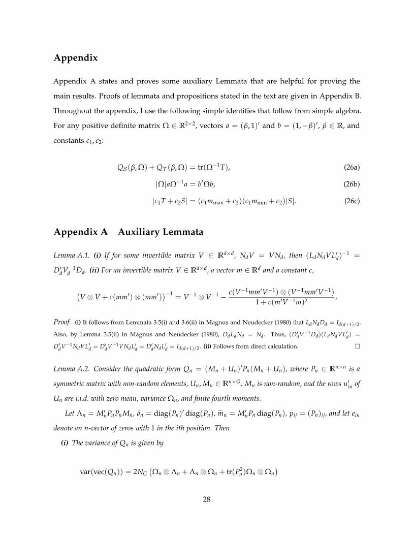
Appendix

Appendix A states and proves some auxiliary Lemmata that are helpful for proving the

main results. Proofs of lemmata and propositions stated in the text are given in Appendix B.

Throughout the appendix, I use the following simple identifies that follow from simple algebra.

For any positive definite matrix Ω ∈ R2×2, vectors a = (β, 1)′ and b = (1,−β)′, β ∈ R, and

constants c1, c2:

QS (β, Ω) + QT (β, Ω) = tr(Ω−1T), (26a)

|Ω|aΩ−1a = b′Ωb, (26b)

|c1T + c2S| = (c1mmax + c2)(c1mmin + c2)|S|. (26c)

Appendix A Auxiliary Lemmata

Lemma A.1. (i) If for some invertible matrix V ∈ Rd×d, NdV = VNd, then (LdNdVL′d)−1 =

D′dV−1d Dd. (ii) For an invertible matrix V ∈ Rd×d, a vector m ∈ Rd and a constant c,

(V ⊗V + c(mm′)⊗ (mm′)

)−1= V−1 ⊗V−1 − c(V−1mm′V−1)⊗ (V−1mm′V−1)

1 + c(m′V−1m)2 ,

Proof. (i) It follows from Lemmata 3.5(i) and 3.6(ii) in Magnus and Neudecker (1980) that Ld NdDd = Id(d+1)/2.

Also, by Lemma 3.5(ii) in Magnus and Neudecker (1980), DdLd Nd = Nd. Thus, (D′dV−1Dd)(Ld NdVL′d) =

D′dV−1NdVL′d = D′dV−1VNdL′d = D′d NdL′d = Id(d+1)/2. (ii) Follows from direct calculation.

Lemma A.2. Consider the quadratic form Qn = (Mn + Un)′Pn(Mn + Un), where Pn ∈ Rn×n is a

symmetric matrix with non-random elements, Un, Mn ∈ Rn×G, Mn is non-random, and the rows u′in of

Un are i.i.d. with zero mean, variance Ωn, and finite fourth moments.

Let Λn = M′nPnPn Mn, δn = diag(Pn)′ diag(Pn), mn = M′nPn diag(Pn), pij = (Pn)ij, and let ein

denote an n-vector of zeros with 1 in the ith position. Then

(i) The variance of Qn is given by

var(vec(Qn)) = 2NG(Ωn ⊗Λn + Λn ⊗Ωn + tr(P2

n)Ωn ⊗Ωn)

28

+ δn(E[uinu′in ⊗ uinu′in]− vec(Ωn) vec(Ωn)

′ − 2NGΩn ⊗Ωn)

+ 2NG(Ψ′3 ⊗mn) + 2(Ψ′3 ⊗mn)′NG,

where Ψ3 = E[(uinu′in)⊗ uin], and the last two lines are equal to zero if the distribution of uin is

normal.

(ii) Suppose that (a) var(vec(Qn)) converges, and δn and Λn are bounded; (b) supn E[‖uin‖8] <

∞; (c) ∑ni=1|pii|4 = o(1), ∑n

i=1(

∑nj=1 p2

ij)2

= o(1), and ∑i<j<k<` pik pi`pjk pj` = o(1); and

(d) ∑ni=1‖e′inPn Mn‖4 = o(1). Then:

vec(Qn −M′nPn Mn − tr(Pn)Ωn)⇒ N (0, limn→∞

(var(vec(Qn)))).

Proof. Proof of Part (i) follows from a tedious, but straightforward calculation. Proof of Part (ii) is a generalization

of the central limit theorems in Chao et al. (2012) and Hansen et al. (2008), and is proved using similar arguments.

Full proof is given in the supplemental appendix.

Lemma A.3. Let Pn = (An + νnBn)/√

mn, where mn → ∞ as n → ∞, νn = O(1), An, Bn ∈ Rn×n

are projection matrices such that AnBn = 0, and for j > 1, tr(An/mjn) = o(1) and tr(νnBn/mj

n) =

o(1). Then condition (ii)c of Lemma A.2 holds.

Proof. Denote the (i, j) elements of An and Bn by aij and bij. The first condition follows from the bound, for

j > 2, ∑i pjii ≤ 2j−1(∑i aj

ii + νjn ∑i bj

ii)/mj/2n ≤ 2j−1(∑i aii + ν

jn ∑i bii)/mj/2

n = o(1) The second condition follows

from ∑i(

∑j p2ij)2 ≤ ∑i

(2 ∑j a2

ij + 2ν2n ∑j b2

ij)2/m2

n = ∑i(2aii + 2ν2

nbii)2/m2

n = o(1).

It therefore remains to show that ∑i<j<k<` pik pi`pjk pj` = o(1). This can be shown using arguments similar to

those in the proof of Lemma B.2 in Chao et al. (2012). Let D denote a diagonal matrix with elements Dii = (Pn)ii,

let Sn = ∑i<j<k<`(pik pi`pjk pj` + pij pi`pjk pk` + pij pik pj`pk`), and let ‖·‖F denote the Frobenius norm. Note that

‖(Pn − D)2‖F ≤ ‖P2n‖F + ‖D2‖F + 2‖DPn‖F = o(1), (27)

where the last equality follows from ‖D2‖2F = ∑i p4

ii = o(1), ‖P2n‖

2F = (tr An + ν4

n tr Bn)/m2n = o(1), and ‖DPn‖2

F =

∑i p2ii ∑j p2

ij ≤ m−2n ∑i(aii + νnbii)(aii + ν2

nbii) = o(1). On the other hand, expanding the left-hand side in (27) yields

‖(Pn − D)2‖2F = 2 ∑

i<jp4

ij + 4 ∑i<j<`

(p2

ij p2i` + p2

ij p2j` + p2

j`p2i`

)+ 8Sn.

29

Since the first four terms are bounded by ∑i(∑j p2ij)

2 = o(1), it follows that Sn = o(1). Define

∆2 = ∑i<j<k

(pij pikεjεk + pij pjkεiεk

),

∆3 = ∑i<j<k

(pik pjkεiεj

),

and let ∆1 = ∆2 + ∆3. Then

E[∆23] = ∑

i<j<k,`pik pjk pi`pj` = ∑

i<j<kp2

ik p2jk + 2 ∑

i<j<k<`

pik pjk pi`pj` = 2 ∑i<j<k<`

pik pjk pi`pj` + o(1),

E[∆21] = tr((Pn − D)4)− 2 ∑

i<jp4

ij = o(1),

E[∆22] = ∑

i<j<k(p2

ij p2ik + p2

ij p2jk) + 2Sn = o(1).

Thus, by the Cauchy-Schwarz inequality,

E[∆23] ≤ 2E[∆2

1] + 2E[∆22] = o(1),

which proves the result.

Corollary A.1. Consider the model (1)–(2), and suppose Assumptions PR, N and MI hold. Then:

√n vec (S−Ω)⇒ N4

(0,

11− αk − α`

2N2(Ω⊗Ω)

)√

n vec(

T − αkΩ− λn

a′Ω−1aaa′)⇒ N4 (0, 2N2(αkΩ⊗Ω + Ω⊗M + M⊗Ω)) ,

where M = λa′Ω−1a aa′.

Proof. The result follows from Lemmata A.2 and A.3, with Pn = (I − ZZ′ −W(W ′W)−1W)/√

n, and Pn =

(ZZ′)/√

n.

Corollary A.2. Consider the model (1)–(2), and suppose Assumption MI(i)–(iii), and Assumption RC

hold, Ξn = Ξ + o(1) where Ξ is a positive semi-definite matrix with Ξ22 > 0, and that (π1,n −

π2,nβn)′Z′ diag(H)/√

nkn = µ + o(1) for some µ. Let m = (µ + µ(Ξ12/Ξ22), µ)′. Then

√n vec(T − (kn/n)S− Ξn)⇒ N (0, ∆),

30

where

∆ = 2N2 (Ω⊗ Ξ + Ξ⊗Ω + (αk(1− α`)/(1− αk − α`)− αkδ)Ω⊗Ω)

+ αkδ(E[viv′i ⊗ viv′i]− vec(Ω) vec(Ω)′

)+ α1/2

k (2N2(Ψ′3 ⊗m) + (Ψ′3 ⊗m)′N2),

and Ψ3 = E[(viv′i)⊗ vi].

Proof. The result follows from Lemmata A.2 and A.3, with Pn = H/√

n.

Appendix B Proofs

Proof of Lemma 1. To ensure that the densities of T and Π are expressed with respect to compatible dominating

measures, I will express the density of T with respect to the measure

µT(dt) =nkn πkn−1/2

Γ(kn/2)Γ((kn − 1)/2)|t|(kn−3)/2λ(dt),

where λ is the Lebesgue measure on the sample space of T, and Γ denotes the gamma function. µT is the

measure induced by the Lebesgue measure µ on the sample space of Π in the sense that for any measurable set B,

µT(B) = µ(δ−1(B)), where δ(Π) = Π′Π/n is the function defining T (Eaton, 1989, Example 5.1). The statistic T has

the same distribution as the statistic WN in Moreira (2009, Section 4), with the parameters λN and Σ in that paper

corresponding to λn/(a′Ω−1a) and Ω. Hence, by Theorem 4.1 in Moreira (2009), the density of T with respect to

µT is given by

fT(T | β, λn, Ω) = K1e−n2 (λn+tr(Ω−1T))|Ω|−kn/2(nλ1/2

n QT (β, Ω)1/2)−kn−2

2 I(kn−2)/2(nλ1/2n QT (β, Ω)1/2), (28)

where K1 = Γ(kn/2)π−kn 2−kn/2−1 and Iν(·) is modified Bessel function of the first kind of order ν. Iν(·) has the

integral representation (Abramowitz and Stegun, 1965, Equation 9.6.18, p. 376)

Iν(t) =(t/2)ν

π1/2Γ(ν + 1/2)G2ν+2(t), where Gk(t) =

∫[−1,1]

ets(1− s2)(k−3)/2 ds.

The density (28) can therefore be written as:

fT(T | β, λn, Ω) =2−kn Γ(kn/2)

πkn+1/2Γ((kn − 1)/2)· e−

n2 (λn+tr(Ω−1T))|Ω|−kn/2Gkn (nλ1/2

n QT (β, Ω)1/2).

Combining this expression with the density for S (with respect to Lebesgue measure), which is given by

fS(S; Ω) = Cn−kn−`n · |S|(n−kn−`n−3)/2|Ω|−n−kn−`n/2e−

n−kn−`n2 tr(Ω−1S),

31

where

C−1ν = (2/ν)νπ1/2Γ(ν/2)Γ((ν− 1)/2) (29)

yields the invariant likelihood

Linv,n(β, λn, Ω; S, T) =2−kn Γ(kn/2)

πkn+1/2Γ((kn − 1)/2)· e−

n2 (λn+tr(Ω−1T))|Ω|−kn/2Gkn (nλ1/2

n QT (β, Ω)1/2) · fS(S; Ω)

∝ exp[−1

2

((n− `n) log|Ω|+ tr(Ω−1S) + nλn − 2 log Gkn (n

√λnQT (β, Ω))

)],

(30)

where S = (n− kn − `n)S + nT. The derivative with respect to Ω is given by:

∂ logLinv,n

∂Ω=

12

Ω−1

[S− (n− `n)Ω−

G′kn(n√

λnQT (β, Ω))

Gkn (n√

λnQT (β, Ω))

nλ1/2n

QT (β, Ω)1/2

(T − QS (β, Ω)

b′ΩbΩbb′Ω

)]Ω−1, (31)

where the derivative ∂QT (β, Ω)/∂Ω is computed using the identity (26a). Note that b′Ωb > 0 for Ω positive

definite, QT (β, Ω) > 0 with probability one for Ω positive definite, and Gkn (t) > 0 for t > 0 (Abramowitz and

Stegun, 1965, p. 374), so that the denominators in (31) are non-zero at any point in the parameter space for (β, Ω, λn)

with probability one.

Fix λn. Denote the ml estimates of β and Ω given λn by (βλn , Ωλn ). Since G(·) is a monotone increasing

function, it follows from (30) that:

βλn = argmaxβ

QT (β, Ωλn ) = argminβ

QS (β, Ωλn ). (32)

Secondly, the derivative (31) evaluated at (βλn , Ωλn ) has to be equal to zero. Pre-multiplying and post-multiplying

Equation (31) by b′λnΩλn and Ωλn bλn therefore yields

(n− `n)b′λnΩλn bλn = b′λn

Sbλn . (33)

Therefore,

βλn = argminβ

QS (β, Ωλn ) = argminβ

QS (β, S) = argmin QS (β, S) = βliml,

where the first equality follows by (32), the second by (33), the third by QS (β, S)−1 = (n− kn − `n)QS (β, S)−1 + n,

and the last equality follows from definition of βliml. By similar arguments, Equations (32) and (33) must also hold

when the likelihood is maximized over λn as well, so that βinv = βliml.

It remains to show (13). This result follows from the fact that Fωn corresponds to the invariant prior distribution

induced by the Haar probability measure νH on O(kn) (which is unique since O(kn) is compact) via the group

action ωn 7→ gωn, g ∈ O(kn), in the sense that for any measurable set B, Fωn (B) = νH(g−1B), and arguments in

Eaton (1989, pp. 87–88). For convenience, I give a direct argument. Since

vec(Π) ∼ N2kn

((a′Ω−1a/n)−1/2a⊗ ηn, Ω⊗ Ikn

),

32

it follows that the limited information likelihood is given by

Lli,n(β, ωn, λn, Ω) = (2π)−kn |Ω|−kn2 e−

n2 (tr(TΩ−1)+λn)en

√λnQT (β,Ω)ω′n A(β,Ω,Π) fS(S; Ω),

where A(β, Ω, Π) = ΠΩ−1a(na′Ω−1aQT (β,Ω))1/2 . To integrate the likelihood, we use the result that for all t ∈ R, α ∈ Skn−1,

and kn ≥ 2 (see Stroock, 1999, pp. 88–89)

∫Skn−1

etα′ω dFωn (ω) =Γ(kn/2)

π1/2Γ((kn − 1)/2)Gkn (t),

Applying this result with t = n√

λnQT (β, Ω) and α = A(β, Ω, Π) gives

∫Lli,n(β, ω, λn, Ω)dFωn (ω) =

2−kn Γ(kn/2)πkn+1/2Γ((kn − 1)/2)

|Ω|−kn2 e−

n2 (tr(TΩ−1)+λn)Gkn (nλ1/2

n QT (β, Ω)1/2) · fS(S; Ω),

which in view of (30) completes the proof.

Proof of Proposition 1. Let ν = n − kn − `n, and to prevent clutter, I use the notation (β, λ, Ω) rather than

(βre, λre, Ωre). Consider first maximizing the likelihood with respect to Ω, holding β and λ fixed. Let Ωβ,λ denote

the resulting estimator. The derivative of the log-likelihood with respect to Ω is given by

∂ logLre,n(β, λ, Ω)

∂Ω=

12

[Ω−1SΩ−1 − (n− `n)Ω−1 − d(λ)

(Ω−1TΩ−1 − QS (β, Ω)

b′Ωbbb′)]

,

where S = nT + νS and d(λ) = nλkn/n+λ and the derivative ∂QT (β, Ω)/∂Ω is computed using the identity (26a).

Since the derivative equals zero at Ωβ,λ, this implies

Ω−1β,λS = (n− `n)I2 + d(λ)

(Ω−1

β,λT −QS (β, Ωβ,λ)

b′Ωβ,λbbb′Ωβ,λ

). (34)

Taking a trace on both sides of the equation and using the identity (26a) then yields

tr(Ω−1β,λS)− d(λ)QT (β, Ωβ,λ) = 2(n− `n). (35)

Pre- and post-multiplying Equation (34) by b′Ωβ,λ and b; and by Ωβ,λ and b yields

b′Ωβ,λb = b′Sb/(n− `n),

(n− `n)Ωβ,λb =1

1− d(λ)QS (β, S)(S− d(λ)T)b.

Plugging these expressions back into Equation (34) and pre-multiplying the resulting expression by Ωβ,λ yields

(n− `n)Ωβ,λ = S− d(λ)T +1

b′(S− d(λ)T)bd(λ)QS (β, S)

1− d(λ)QS (β, S)(S− d(λ)T)bb′(S− d(λ)T). (36)

Taking a determinant on both sides of the equation, using the matrix determinant lemma |A + cVV′| = |A|(1 +

33

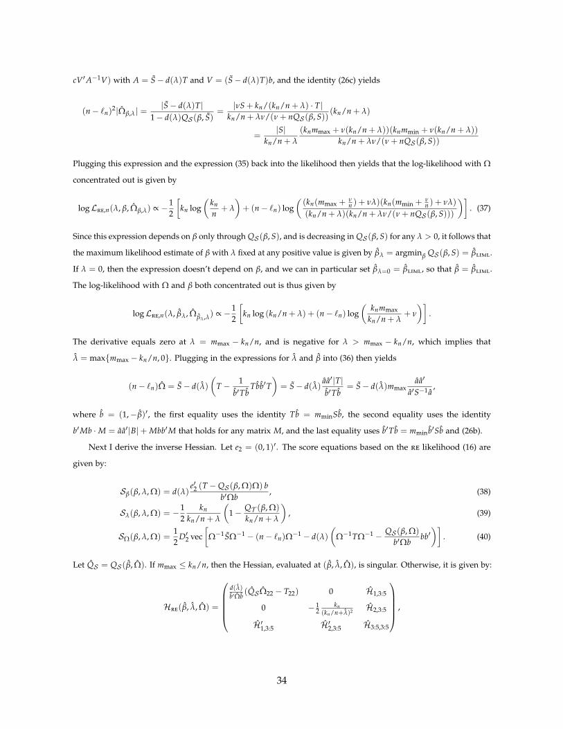
cV′A−1V) with A = S− d(λ)T and V = (S− d(λ)T)b, and the identity (26c) yields

(n− `n)2|Ωβ,λ| =

|S− d(λ)T|1− d(λ)QS (β, S)

=|νS + kn/(kn/n + λ) · T|

kn/n + λν/(ν + nQS (β, S))(kn/n + λ)

=|S|

kn/n + λ

(knmmax + ν(kn/n + λ))(knmmin + ν(kn/n + λ))

kn/n + λν/(ν + nQS (β, S))

Plugging this expression and the expression (35) back into the likelihood then yields that the log-likelihood with Ω

concentrated out is given by

logLre,n(λ, β, Ωβ,λ) ∝ −12

[kn log

(kn

n+ λ

)+ (n− `n) log

((kn(mmax +

νn ) + νλ)(kn(mmin + ν

n ) + νλ)

(kn/n + λ)(kn/n + λν/(ν + nQS (β, S)))

)]. (37)

Since this expression depends on β only through QS (β, S), and is decreasing in QS (β, S) for any λ > 0, it follows that

the maximum likelihood estimate of β with λ fixed at any positive value is given by βλ = argminβ QS (β, S) = βliml.

If λ = 0, then the expression doesn’t depend on β, and we can in particular set βλ=0 = βliml, so that β = βliml.

The log-likelihood with Ω and β both concentrated out is thus given by

logLre,n(λ, βλ, Ωβλ ,λ) ∝ −12

[kn log (kn/n + λ) + (n− `n) log

(knmmax

kn/n + λ+ ν

)].

The derivative equals zero at λ = mmax − kn/n, and is negative for λ > mmax − kn/n, which implies that

λ = maxmmax − kn/n, 0. Plugging in the expressions for λ and β into (36) then yields

(n− `n)Ω = S− d(λ)(

T − 1b′Tb

Tbb′T)= S− d(λ)

aa′|T|b′Tb

= S− d(λ)mmaxaa′

a′S−1 a,

where b = (1,−β)′, the first equality uses the identity Tb = mminSb, the second equality uses the identity

b′Mb ·M = aa′|B|+ Mbb′M that holds for any matrix M, and the last equality uses b′Tb = mminb′Sb and (26b).

Next I derive the inverse Hessian. Let e2 = (0, 1)′. The score equations based on the re likelihood (16) are

given by:

Sβ(β, λ, Ω) = d(λ)e′2 (T −QS (β, Ω)Ω) b

b′Ωb, (38)

Sλ(β, λ, Ω) = −12

kn

kn/n + λ

(1− QT (β, Ω)

kn/n + λ

), (39)

SΩ(β, λ, Ω) =12

D′2 vec[

Ω−1SΩ−1 − (n− `n)Ω−1 − d(λ)(

Ω−1TΩ−1 − QS (β, Ω)

b′Ωbbb′)]

. (40)

Let QS = QS (β, Ω). If mmax ≤ kn/n, then the Hessian, evaluated at (β, λ, Ω), is singular. Otherwise, it is given by:

Hre(β, λ, Ω) =

d(λ)b′Ωb

(QS Ω22 − T22) 0 H1,3:5

0 − 12

kn(kn/n+λ)2 H2,3:5

H′1,3:5 H′2,3:5 H3:5,3:5

,

34

where

H1,3:5 =12

d(λ)QSb′Ωb

(2

e′2Ωbb′Ωb

b⊗ b− b⊗ e2 − e2 ⊗ b

)′D2,

H2,3:5 =12

kn

(kn/n + λ)2

(QSbΩb

b⊗ b− vec(Ω−1TΩ−1)

)′D2 = −1

2kn

(kn/n + λ)2mmax

aS−1 a

(Ω−1 a⊗ Ω−1 a

)′D2,

H3:5,3:5 = − (n− `n)

2D′2

((Ω−1 − cbb′

b′Ωb

)⊗(

Ω−1 − cbb′

b′Ωb

)− (2c− c2)

bb′

b′Ωb⊗ bb′

b′Ωb

)D2.

By the formula for block inverses, the upper 2× 2 submatrix of the inverse Hessian is given by:

H1:2,1:2(β, λ, Ω) =(H1:2,1:2 − H1:2,3:5H−1

3:5,3:5H′1:2,3:5

)−1. (41)

Applying Lemma A.1 and using the fact that Nd(A⊗ A) = Nd(A⊗ A)Nd = (A⊗ A)Nd (Magnus and Neudecker,

1980, Lemma 2.1(v)) yields:

H−13:5,3:5 = − 2

n− `nL2N2

[(Ω +

c1− c

Ωbb′Ωb′Ωb

)⊗(

Ω +c

1− cΩbb′Ωb′Ωb

)+

c2 − 2c(1− c)2

Ωbb′Ω⊗ Ωbb′Ω(b′Ωb)2

]N2L′2,

It follows that

H1,3:5H−13:5,3:5H

′1,3:5 = − (n− `n)c2

1− c|Ω|

(b′Ωb)2 .

Finally, since H2,3:5H−13:5,3:5H′1,3:5 = 0, Equation (41) combined with the expression in the previous display yields

H11re

=(H11 − H1,3:5H−1

3:5,3:5H′1,3:5

)−1=

b′Ωb(λ + kn/n)nλ

(QS Ω22 − T22 +

c1− c

QSa′Ω−1 a

)−1

,

which yields the result.

It remains to show that the inverse Hessian is consistent for Vliml,N . To this end, note that mmin = b′

limlTbliml

b′liml

Sbliml

p→

αk by Corollary A.1 and consistency of β. By continuity of the trace operator, and Corollary A.1

mmax = tr(S−1T)−mmin = tr(S−1T)− b′liml

Tbliml

b′liml

Sbliml

p→ 2αk + λ− αk = λ + αk.

Consistency of Ω then follows by consistency of λ and β, Corollary A.1, and Slutsky’s Theorem. It also follows that

QS = (n− `n)b′Tbb′Sb

=(n− `n)b′Tb

(n− kn − `n)b′Sb + nb′Tb=

(1

1− `n/n+

n− kn − `n

(n− `n)mmin

)−1 p→ αk.

Hence,c

1− cp→ αkλ

αk(1− α`) + (1− αk − α`)λ,

35

so that

−nH11re

p→ − b′Ωb(αK + λ)

λ

(− λ

a′Ω−1a+

λα2K

a′Ω−1a ((1− αK − α`)λ + (1− α`)αK)

)−1

=b′Ωba′Ω−1a

λ2

(λ +

(1− α`)αK1− α` − αK

)= V

liml,N ,

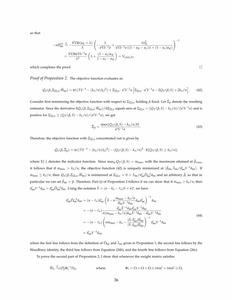
which completes the proof.

Proof of Proposition 2. The objective function evaluates as:

Qn(β, Ξ22,n; Wre) = tr((TS−1 − (kn/n)I2)2) + Ξ22,n · a′S−1a

[Ξ22,n · a′S−1a− 2QT (β, S) + 2kn/n

]. (42)

Consider first minimizing the objective function with respect to Ξ22,n, holding β fixed. Let Ξβ denote the resulting

estimator. Since the derivative ∂Qn(β, Ξ22,n; Wre)/∂Ξ22,n equals zero at Ξ22,n = (QT (β, S)− kn/n)/(a′S−1a) and is

positive for Ξ22,n ≥ (QT (β, S)− kn/n)/(a′S−1a), we get

Ξβ =maxQT (β, S)− kn/n, 0

a′S−1a. (43)

Therefore, the objective function with Ξ22,n concentrated out is given by

Qn(β, Ξβ) = tr((TS−1 − (kn/n)I2)2)− (QT (β, S)− kn/n)2 · 1QT (β, S) ≥ kn/n,

where 1· denotes the indicator function. Since maxβ QT (β, S) = mmax, with the maximum attained at βliml,

it follows that if mmax > kn/n, the objective function (42) is uniquely minimized at (βre, λre/a′re

S−1 are). If

mmax ≤ kn/n, then Qn(β, Ξ22,n; Wre) is minimized at Ξ22,n = 0 = λre/a′re

Ω−1re

are and an arbitrary β, so that in

particular we can set βre = β. Therefore, Part (i) of Proposition 2 follows if we can show that if mmax > kn/n, then

a′re

S−1 are = a′re

Ω−1re

are. Using the notation S = (n− kn − `n)S + nT, we have

a′re

Ω−1re

are = (n− `n)a′re

(S− n

mmax − kn/na′

reS−1 are

are a′re

)−1are

= −(n− `n)a′

reS−1 are a′

reS−1 are

n(mmax − kn/n)areS−1 are − a′re

S−1 are

= −(n− `n)

(nmmax − kn −

|S||S|

b′re

Sbre

breSbre

)−1

a′re

S−1 are

= a′re

S−1 are,

(44)

where the first line follows from the definition of Ωre and λre given in Proposition 1, the second line follows by the

Woodbury identity, the third line follows from Equation (26b), and the fourth line follows from Equation (26c).

To prove the second part of Proposition 2, I show that whenever the weight matrix satisfies

Wnp→cD′2Φ−1

t D2, where Φt = Ω⊗Ω + Ω⊗ tmm′ + tmm′ ⊗Ω,

36

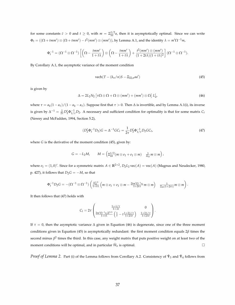
for some constants c > 0 and t ≥ 0, with m = Ξ1/222 a, then it is asymptotically optimal. Since we can write

Φt = ((Ω + tmm′)⊗ (Ω + tmm′)− t2(mm′)⊗ (mm′)), by Lemma A.1, and the identity λ = m′Ω−1m,

Φ−1t = (Ω−1 ⊗Ω−1)

[(Ω− tmm′

1 + tλ

)⊗(

Ω− tmm′

1 + tλ

)+

t2(mm′)⊗ (mm′)(1 + 2tλ)(1 + tλ)2

](Ω−1 ⊗Ω−1).

By Corollary A.1, the asymptotic variance of the moment condition

vech(T − (kn/n)S− Ξ22,naa′) (45)

is given by

∆ = 2L2N2[τΩ⊗Ω + Ω⊗ (mm′) + (mm′)⊗Ω

]L′2, (46)

where τ = αk(1− α`)/(1− αk − α`). Suppose first that τ > 0. Then ∆ is invertible, and by Lemma A.1(i), its inverse

is given by ∆−1 = 12τ D′2Φ−1

1/τ D2. A necessary and sufficient condition for optimality is that for some matrix Ct

(Newey and McFadden, 1994, Section 5.2),

(D′2Φ−1t D2)G = ∆−1GCt =

12τ

D′2Φ−11/τ D2GCt, (47)

where G is the derivative of the moment condition (45), given by:

G = −L2 M, M =(

Ξ1/222 (m⊗ e1 + e1 ⊗m) 1

Ξ22m⊗m

),

where e1 = (1, 0)′. Since for a symmetric matrix A ∈ R2×2, D2L2 vec(A) = vec(A) (Magnus and Neudecker, 1980,

p. 427), it follows that D2G = −M, so that

Φ−1t D2G = −(Ω−1 ⊗Ω−1)

(Ξ1/2

221+tλ

(m⊗ e1 + e1 ⊗m− 2tm′Ω−1e1

1+2tλ m⊗m)

1Ξ22(1+2tλ)m⊗m

).

It then follows that (47) holds with

Ct = 2τ

1+λ/τ1+λt 0

2m′Ω−1e1Ξ3/2

1+tλ

(1τ − t 1+2λ/τ

1+2λt

)1+2λ/τ1+2λt

.

If τ = 0, then the asymptotic variance ∆ given in Equation (46) is degenerate, since one of the three moment

conditions given in Equation (45) is asymptotically redundant: the first moment condition equals 2β times the

second minus β2 times the third. In this case, any weight matrix that puts positive weight on at least two of the

moment conditions will be optimal, and in particular Wn is optimal.

Proof of Lemma 2. Part (i) of the Lemma follows from Corollary A.2. Consistency of Ψ3 and Ψ4 follows from

37

Lemma A.7 in Anatolyev (2013). Finally, since ZZ′ is a projection matrix, ‖ZZ′ diag(H)‖ ≤ ‖diag(H)‖, so that

var(µ) =1

nknΩ22‖ZZ′ diag(H)‖2 ≤ 1

nknΩ22 diag(H)′ diag(H) =

Ω22n

δ(1 + o(1)) = o(1).

Thus, µp→ µ by Markov inequality.

Proof of Proposition 3. It follows by Corollary A.2 and the Delta method that

√n(

βumd − Ξ12,n/Ξ22,n)⇒ N (0, Vumd),

where, letting A = (e2b′ + be′2)/2Ξ22, e2 = (0, 1)′,

Vumd = vec(A)′∆ vec(A)

= tr(4AΩAΞ + 2τAΩAΩ) + αkδ(

E[(v′i Avi)2]− tr(ΩA)2 − 2 tr(AΩAΩ)

)+ 4α1/2

k (µ + µβ, µ)E[Aviv′i Avi]

= Vliml,N +

2τ(e′2Ωb)2 + 2α1/2k µE[v2iε

2i ] + αkδ(E[v2

2iε2i ]− 3(e′2Ωb)2 − |Ω|)

Ξ222

+Ω22|Ξ|/Ξ22 + 2α1/2

k µE[v22iεi]

Ξ222

= Vliml +(2τ + αkδκ)(e′2Ωb)2 + 2γ

(αkδE[(v2i − γεi)ε

3i ] + α1/2

k µE[ε3i ])

Ξ222

+Ω22|Ξ|/Ξ22 + 2α1/2

k µE[v22iεi]

Ξ222

,

from which the result follows.

Proof of Proposition 4. We have:

(mmin − αk) =b′

liml(T − αkS)bliml

b′liml

Sbliml

=b′

liml(T − αkS− λnaa′/(a′Ω−1a))bliml

b′liml

Sbliml

+λn(a′ bliml)2

(a′Ω−1a)b′liml

Sbliml

=(bliml ⊗ bliml)′ vec

(T − αkS− λnaa′/(a′Ω−1a)

)b′

limlSbliml

+λn(bliml − β)2

(a′Ω−1a)b′liml

Sbliml

=(bliml ⊗ bliml)′ vec (T − (kn/n)S− Ξ22,naa′)

b′liml

Sbliml

+ Op(n−1)

=(b⊗ b)′ vec (T − (kn/n)S− Ξ22,naa′)

b′Ωb+ Op(n−1),

where the first line follows from the identity mmin = QS (βliml, S), the second and third line follows by algebra, the

fourth line and the last line follow from√

n-rate of convergence βliml and T − (kn/n)S. Expanding the numerator

then yields

n√kn

(mmin − αk) =(b⊗ b)′ vec(V′(H/

√kn)V)

b′Ωb+ Op(k−1/2

n ) =ε′(H/

√kn)ε

b′Ωb+ Op(k−1/2

n ).

If kn → ∞, then by Lemmata A.2 and A.3, with Pn = H/√

kn,

n√kn

(mmin − αk)⇒ N (0, 2(1− α`)/(1− αk − α`) + δκ).

38

If kn = K is fixed, then vec(Π −Π) = ∑i vi ⊗ zi ⇒ N (0, Ω · IK), since the Lyapunov condition is implied by

∑ni=1‖zi‖2+ν = ∑i(ZZ′)1+ν/2

ii ≤ maxi(ZZ′)ν/2ii tr(ZZ′) = o(1) for any ν > 0. It then follows by standard arguments

that nmmin ⇒ χ2K−1, which proves the first part.

To prove the second part, I use the approximation from Peiser (1943) (see also Anatolyev and Gospodinov,

2011) that as k→ ∞,

qχ2k

1−ns = k + Φ−1(1− ns)√

2k + O(1),

where qχ2k

1−ns denotes the 1− ns quantile of a χ2 distribution with k degrees of freedom. Therefore, if kn → ∞,

letting c = Φ(√

(1−αk)1−αk−α`

+ δκ2 Φ−1(ns))

P

(nmmin ≥ q

χ2kn−1

1−c

)= P

(nmmin/

√kn ≥

√kn + Φ−1(1− c)

√2 + o(1)

)= P

(nmmin/

√kn −

√kn ≥ Φ−1(1− c)

√2 + o(1)

)= P

(N (0, 1) + op(1) ≥ Φ−1(1− c)

√2(1− αk − α`)

2(1− α`) + (1− αk − α`)δκ+ o(1)

)

= Φ

(Φ−1(c)

√2(1− αk − α`)

2(1− α`) + (1− αk − α`)δκ

)+ o(1)

= ns + o(1).

If kn is fixed, then, since ∑ni=1(ZZ′)2

ii ≤ maxj(ZZ′)jj tr(ZZ′), it follows that δn = ∑ni=1(ZZ′)2

ii/kn + o(1) = o(1).

Thus, c = ns + o(1), and so P

(nmmin ≥ q

χ2kn−1

1−c

)= ns + o(1). Since δn and κ are consistent estimators of δ and κ,

the assertion of the theorem follows.

References

Abramowitz, M. and Stegun, I. A. (eds.) (1965). Handbook of Mathematical Functions: with Formulas, Graphs, and

Mathematical Tables. New York: Dover. 31, 32

Aizer, A. and Doyle, J. J., Jr. (2015). Juvenile incarceration, human capital, and future crime: Evidence from

randomly assigned judges. The Quarterly Journal of Economics, 130 (2), 759–803. 20

Anatolyev, S. (2013). Instrumental variables estimation and inference in the presence of many exogenous regressors.

The Econometrics Journal, 16 (1), 27–72. 4, 7, 18, 38

— and Gospodinov, N. (2011). Specification testing in models with many instruments. Econometric Theory, 27 (2),

427–441. 4, 25, 26, 39

Anderson, T. W., Kunitomo, N. and Matsushita, Y. (2010). On the asymptotic optimality of the LIML estimator

with possibly many instruments. Journal of Econometrics, 157 (2), 191–204. 4, 18, 19

39

— and Rubin, H. (1949). Estimation of the parameters of a single equation in a complete system of stochastic

equations. The Annals of Mathematical Statistics, 20 (1), 46–63. 8

Andrews, D. W. K., Moreira, M. J. and Stock, J. H. (2006). Optimal two-sided invariant similar tests for

instrumental variables regression. Econometrica, 74 (3), 715–752. 9

—, — and — (2008). Efficient two-sided nonsimilar invariant tests in iv regression with weak instruments. Journal of

Econometrics, 146 (2), 241–254. 6

Angrist, J. D., Graddy, K. and Imbens, G. W. (2000). The interpretation of instrumental variables estimators in

simultaneous equations models with an application to the demand for fish. Review of Economic Studies, 67 (3),

499–527. 3, 21

— and Imbens, G. W. (1995). Two-stage least squares estimation of average causal effects in models with variable

treatment intensity. Journal of the American Statistical Association, 90 (430), 431–442. 3, 21

— and Krueger, A. B. (1991). Does compulsory school attendance affect schooling and earnings? The Quarterly

Journal of Economics, 106 (4), 979–1014. 7

Arellano, M. (2003). Panel Data Econometrics. New York, NY: Oxford University Press. 4, 16

Bekker, P. A. (1994). Alternative approximations to the distributions of instrumental variable estimators. Econometrica,

62 (3), 657–681. 2, 4, 7, 8, 9, 15

— and Crudu, F. (2015). Jackknife instrumental variable estimation with heteroskedasticity. Journal of Econometrics,

185 (2), 332–342. 4

Belloni, A., Chen, D., Chernozhukov, V. and Hansen, C. B. (2012). Sparse models and methods for optimal

instruments with an application to eminent domain. Econometrica, 80 (6), 2369–2429. 4

Carrasco, M. (2012). A regularization approach to the many instruments problem. Journal of Econometrics, 170 (2),

383–398. 4

Cattaneo, M. D., Crump, R. K. and Jansson, M. (2012). Optimal inference for instrumental variables regression

with non-gaussian errors. Journal of Econometrics, 167 (1), 1–15. 20

Chamberlain, G. (1982). Multivariate regression models for panel data. Journal of Econometrics, 18 (1), 5–46. 10, 19

— (2007). Decision theory applied to an instrumental variables model. Econometrica, 75 (3), 609–652. 4, 6, 9

— and Imbens, G. W. (2004). Random effects estimators with many instrumental variables. Econometrica, 72 (1),

295–306. 1, 3, 8, 11, 12

— and Moreira, M. J. (2009). Decision theory applied to a linear panel data model. Econometrica, 77 (1), 107–133. 4

40

Chao, J. C., Hausman, J. A., Newey, W. K., Swanson, N. R. and Woutersen, T. (2014). Testing overidentifying

restrictions with many instruments and heteroskedasticity. Journal of Econometrics, 178 (1), 15–21, Annals Issue:

Misspecification Test Methods in Econometrics. 4

— and Swanson, N. R. (2005). Consistent estimation with a large number of weak instruments. Econometrica, 73 (5),

1673–1692. 4

—, —, Hausman, J. A., Newey, W. K. and Woutersen, T. (2012). Asymptotic distribution of jive in a heteroskedastic

iv regression with many instruments. Econometric Theory, 12 (1), 42–86. 4, 29

Chioda, L. and Jansson, M. (2009). Optimal invariant inference when the number of instruments is large. Econometric

Theory, 25 (3), 793–805. 4, 9, 12

Cragg, J. G. and Donald, S. G. (1993). Testing identifiability and specification in instrumental variable models.

Econometric Theory, 9 (2), 222–240. 3, 26

Dobbie, W. and Song, J. (2015). Debt relief and debtor outcomes: Measuring the effects of consumer bankruptcy

protection. American Economic Review, 105 (3), 1272–1311. 20

Donald, S. G. and Newey, W. K. (2001). Choosing the number of instruments. Econometrica, 69 (5), 1161–1191. 3, 21,

22

Eaton, M. L. (1989). Group invariance applications in statistics, Regional conference series in Probability and Statistics,

vol. 1. Hayward, California: Institute of Mathematical Statistics. 9, 31, 32

Gautier, E. and Tsybakov, A. B. (2014). High-dimensional instrumental variables regression and confidence sets,

arXiv:1105.2454. 4

Goldberger, A. S. and Olkin, I. (1971). A minimum-distance interpretation of limited-information estimation.

Econometrica, 39 (3), 635–639. 15

Hahn, J. (2002). Optimal inference with many instruments. Econometric Theory, 18 (1), 140–168. 4, 19

Hansen, C. B., Hausman, J. A. and Newey, W. K. (2008). Estimation with many instrumental variables. Journal of

Business & Economic Statistics, 26 (4), 398–422. 4, 18, 29

Hausman, J. A., Newey, W. K., Woutersen, T., Chao, J. C. and Swanson, N. R. (2012). Instrumental variable

estimation with heteroskedasticity and many instruments. Quantitative Economics, 3 (2), 211–255. 4

Imbens, G. W. and Angrist, J. D. (1994). Identification and estimation of local average treatment effects. Econometrica,

62 (2), 467–475. 21

41

Kolesár, M. (2013). Estimation in instrumental variables models with heterogeneous treatment effects, working

paper, Princeton University. 21

Kolesár, M., Chetty, R., Friedman, J., Glaeser, E. L. and Imbens, G. W. (2015). Identification and inference with

many invalid instruments. Journal of Business & Economic Statistics, 33 (4), 474–484. 7, 9, 21, 22

Kunitomo, N. (1980). Asymptotic expansions of the distributions of estimators in a linear functional relationship

and simultaneous equations. Journal of the American Statistical Association, 75 (371), 693–700. 2, 4

Lancaster, T. (2000). The incidental parameter problem since 1948. Journal of Econometrics, 95 (2), 391–413. 4

— (2002). Orthogonal parameters and panel data. Review of Economic Studies, 69 (3), 647–666. 13

Lee, Y. and Okui, R. (2012). Hahn-Hausman test as a specification test. Journal of Econometrics, 167 (1), 133–139. 26

Magnus, J. R. and Neudecker, H. (1980). The elimination matrix: Some lemmas and applications. SIAM Journal on

Algebraic and Discrete Methods, 1 (4), 422–449. 14, 28, 35, 37

Moreira, M. J. (2003). A conditional likelihood ratio test for structural models. Econometrica, 71 (4), 1027–1048. 8

— (2009). A maximum likelihood method for the incidental parameter problem. The Annals of Statistics, 37 (6A),

3660–3696. 4, 9, 11, 31

Morimune, K. (1983). Approximate distributions of k-class estimators when the degree of overidentifiability is

large compared with the sample size. Econometrica, 51 (3), 821–841. 2, 4

Nagar, A. L. (1959). The bias and moment matrix of the general k-class estimators of the parameters in simultaneous

equations. Econometrica, 27 (4), 575–595. 3, 21

Newey, W. K. and McFadden, D. L. (1994). Large sample estimation and hypothesis testing. In R. F. Engle and D. L.

McFadden (eds.), Handbook of Econometrics, vol. 4, Chapter 36, New York, NY: Elsevier, pp. 2111–2245. 15, 18, 37

Neyman, J. and Scott, E. L. (1948). Consistent estimates based on partially consistent observations. Econometrica,

16 (1), 1–32. 2, 4

Peiser, A. M. (1943). Asymptotic formulas for significance levels of certain distributions. The Annals of Mathematical

Statistics, 14 (1), 56–62. 39

Phillips, P. C. B. (1983). Exact small sample theory in the simultaneous equations model. In Z. Griliches and M. D.

Intriligator (eds.), Handbook of Econometrics, vol. 1, Chapter 8, North Holland, pp. 449–516. 5

Rothenberg, T. J. (1984). Approximating the distributions of econometric estimators and test statistics. In Z. Griliches

and M. D. Intriligator (eds.), Handbook of Econometrics, vol. 2, Chapter 15, New York, NY: North Holland, pp.

881–935. 7

42

Sargan, J. D. (1958). The estimation of economic relationships using instrumental variables. Econometrica, 26 (3),

393–415. 4, 26

Sims, C. A. (2000). Using a likelihood perspective to sharpen econometric discourse: Three examples. Journal of

Econometrics, 95 (2), 443–462. 4

Stroock, D. W. (1999). A Concise Introduction to the Theory of Integration. Boston, MA: Birkhäuser, 3rd edn. 33

van der Ploeg, J. and Bekker, P. A. (1995). Efficiency Bounds for Instrumental Variable Estimators Under Group-

Asymptotics. SOM Research Report 95B24, University of Groningen. 19

van Hasselt, M. (2010). Many instruments asymptotic approximations under nonnormal error distributions.

Econometric Theory, 26 (02), 633–645. 4, 18

Wong, C. S. and Wang, T. (1992). Moments for elliptically contoured random matrices. Sankhya: The Indian Journal

of Statistics, Series B, 54 (3), 265–277. 19

43