MHD FREE AND FORCED CONVECTION FLOW IN AN

INCLINED CHANNEL

4.1. INTRODUCTION:

The problem of free and forced convection resulting from the flow over

a heated inclined flat plates provide probably one of the most fundamental

problems in heat transfer and is thus of considerable theoretical and practical

interest. In spite of the fact that a greater number of analytical and numerical

results are available. It still continues to be a topic of vital importance for

many practical applications, and there by, generating a need for a full

understanding. Convection heat transfer is present in many engineering

applications, such as solar collectors, environmental engineering and

electronic packaging. A large amount of papers were published dealing with

natural convection in two dimensional enclosures, channel and plates,

considering the variation of different parameters, such as Rayleigh number,

Prandtl number, aspect ratio, radiation, conduction, variable properties and

discrete sources. Recently, a wide literature on laminar mixed convection in

both vertical or horizontal channels and tubes has been developed. The main

technical applications of these researches concern cooling systems for

electronic devices and solar energy thermal conversion. Many results

available in the literature are collected in [I]. In particular, the fully developed

mixed convection in vertical channels was studied analytically by Aung and

Worku [26], Aung [14],

The study of magneto-hydrodynamic flow for electrically conducting

fluid pan heated surface has attracted the interest of many researches in view

of its important applications in many engineering problems such as plasma

studies, petroleum industries MHD power generations, cooling of nuclear

rectors the boundary layer control in aerodynamics and crystal growth. Until

recently this study was largely concerned with flow and heat transfer

characteristics in various physical situations. Watanabe and Pop [29]

investigated the heat transfer in the thermal boundary layer of magneto-

hydrodynamic flow over a flat plate. Michiyochi et al. [17] considered natural

convection heat transfer from a horizontal cylinder to the mercury under a

magnetic field. Vajravelu and Nayfeh [28] studied hydro magnetic convection

at a cone and a wedge. The study of hydro magnetic dynamic free convection

through a viscous fluid past a semi- infinite plate is considered very essential

to understand the behaviour of the performance of the fluid motion in several

applications. It serves as the basis for understanding some of the important

phenomena occurring in heat exchange devices. MHD free convection flows

past a semi- infinite vertical plate have been studied in different physical

condition by sparrow and Cess [ 5 ] , Riley [18] aid others.

The Problems mentioned above are concerned with thermal convection

only. But in nature along with free convection currents caused by the

temperature differences, the flow is also affected by the differences in material

constitution, for example, in atmospheric flows there exist differences in H20

concentration and hence the flow is affected by such concentration difference.

In many engineering applications, the foreign gases are injected. This causes

a reduction in wall shear stress, the mass transfer conductance or the rate of

heat transfer, Usually, H20, COz etc are the foreign gases, which are injected

in the air flowing past bodies. The effects of foreign mass, also know as

diffusing species concentration were studied under different conditions by

Somers [2], Mathers et a1. [lo], and others either by integral method or by

asymptotic analysis. But the first systematic study of mass transfer effects on

free convection flow past a semi infinite vertical plate was presented by

Gebhart and Pera [13] who presented a similarity solution to this problem and

introduced a parameter N which is a measwe of relative importance of

chemical and thermal diffusion causing a density difference that drives the

flow the parameter N is positive when both effects combined to drive the flow

and it is negative when these effects are opposed. Unsteady free convective

flow on taking into account the mass transfer phenomenon past an infinite

vertical porous late with constant such on was studies by Soundalgekar and

Wavre [I 91.

Callahan and Marner [16] first considered the transient free convection

flow past a semi infinite plate by explicit finite difference method. They also

considered the presence of species concentration. However this analysis is not

applicable for other fluids whose Prandtl number is different h m unity.

Soundalgekar and Ganesan [20] analyzed transient free convective flow past a

semi infinite vertical flat plate, taking into account mass transfer by an

implicit finite difference method of Crank-Nicolson type. In their analysis

they observed that an increase in the N leads to an increase in the velocity but

a decrease in the temperature and concentration. Elbashbeshy 1321 studied

heat and mass transfer along a vertical plate with variable surface temperature

and concentration in the presence of magnetic field. Adoeldahab and

Elbarbary [37] took into account the Hall current effect on the MHD free

convection heat and mass transfer over a semi infinite vertical plate upon

which the flow subjected to a strong external magnetic field. Chen [40]

studied heat and mass transfer in MHD flow by natural convection from a

permeable inclined surface with variable temperature and concentration using

Keller box finite difference method and found that an increase in the value of

temperature exponent m leads to a decrease in the local skin friction, Nusselt

and Sherwood numbers. Takhar et al. [33] considered the unsteady Eree

convection flow over a semi infinite vertical plate. Ganesan and Rani [35]

studied the unsteady free convection on vertical cylinder with variable heat

and mass flux.

In this chapter, the fully developed and laminar free and forced

convection with MHD in an inclined channel is studied. The flow is assumed

to be steady and fully developed. The walls are kept at different uniform

temperatures. Expressions for velocity, bulk temperature and Pressure

gradient are obtained for different cases of ' 4 ' . The effects of magnetic

Gr parameter M, Ratio of Grashoff number \ and Reynolds number(-), the

Re

- pressure gradienta =A, ratio of wall temperature differences (rr) are

cix

studied on velocity and bulk temperature and the results are discussed through

graphs.

4.2. NOMENCLATURE:

P : Fluid pressure

p : Fluid density

u : Kinematic viscosity

g : Acceleration due to gravity

p : Thermal expansion co efficient

h : Spacing between two walls

G, : Grashoff number.

R, : Reynolds number.

P* : Dimensionless pressure difference.

r~ : Wall temperature difference ratio.

113

: Angle of the inclination of the channel to

horizontal

: Coefficient of viscosity

: Ambient temperature

: Velocity vector

: Temperature at the wall x=-h

: Temperature at the wall x=h/2

: Axial velocity

: Dimension less velocity =U/W

: Axial transverse coordinates

: Dimensionless axial coordinate

: Dimensionless transverse coordinate

: Dimensionless temperature

: Bulk temperature

: Pressure gradient

: Electric conductivity

: Magnetic field

: Dimensionless velocities of the plates

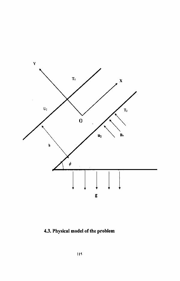
4.3. Physical model of the problem

4.4. FORMATION OF THE PROBLEM:

The steady laminar fiee and forced convection flow between two

parallel flat plates in an inclined channel is considered. Let the inclination

of the channel to the horizontal be ' 4 '. Let the x- axis (the flow

direction) be taken mid way between the plates and the y- axis is taken

perpendicular to the plates. The plates are maintained at different uniform

temperatures. The distance between the plates is taken to be 'h' and the

walls are moving with the velocities uI&u2 respectively. A uniform

transverse magnetic field is applied perpendicular to the plate. The form of

the flow is given in the figure.

The following assumptions are made in the analysis of the problem.

(i) The fluid is Newtonian, viscous, and incompressible.

(ii) The flow is steady and the Grashoff number is small.

(iii) The velocity 'u 'in the axial direction is a function of y and #only.

(iv) The heat transfer takes place by conduction and hence the temper is

linear in 'y'.

(v) The gravitational force 'g' is taken into account and the pressure is a

function of x and y only.

(vi) The channel height is much larger than the channel spacing, so that

the velocity component u in y- direction is taken as zero in the entire

cross section of the flow.

(vii) Energy dissipation is neglected.

(viii) The magnetic Reynolds number is taken to be small enough so that

the induced magnetic field is negligible compared to the applied

magnetic field.[6]

(ix) Electric field is neglected[3]

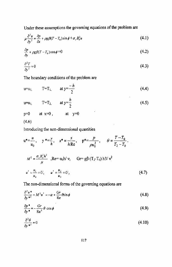
Under these assumptions the governing equations of the problem are

a 2 T -0 -... @ 2

The boundary conditions of the problem are

p=O at x=O, at y=O

(4.6)

Introducing the non-dimensional quantities

The non-dimensional forms of the governing equations are

Where o = -*=pressure gradient dx

The boundary conditions are

4.5. SOLUTION OF THE PROBLEM:

Solving the equation (4.10) subjected to the boundary conditions

(4.12) & (4.13)

and reverting the parameters, we get the fully developed temperature

profile

. I t r T 8=(1-r , )y+(- )

2 (4.1 4)

Solving equation (4.9) using the equations (4.12), (4.13), & (4.14), we get

Solving equation (4.8) using the equations (4.12), (4.13), & (4.14), we get

u = ------ - a - Bs in@ As in4 sinh My Ice:" A42cosy]c"h"t[2M2sin h y ~ : ] (4.16)

To evaluate the parameter ' a ' an additional equation expressing the

global conservation of mass at any cross section in the channel is also

required.

2

For this )udY = 1 in the dimension less form (4.17) -I - 2

Employing equation (4.16) into equation (4.17), we have

hM hM M cos--- - 2k sin -

2 Bsinb a = M ' [ hM

t-] hM M 2

M cos - 2 sin - 2 2

Using equation (4.18) in equation (4.16), we get the following velocity

Gr distribution at any value of -, rr,

Re

4.5.1 Velocity

k, u = - hM

coshMy-- cos -

hM sin -

2 2

sin

(4.19)

4-52 Bulk Temperature Ob

).@9 -1 - 2 The bulk temperature is defined as 8, =- (4.20)

Using equations (4.14) & (4.19) in equation (4.20) we get the expression

for bulktemperature

hM 2k, A? sin -

[McoshM-2sin'M]+ Oh = ------- - hM hM 2 2

Mcos- M* sin--- 2 2

2 ~ ' sin ---

2 sin --

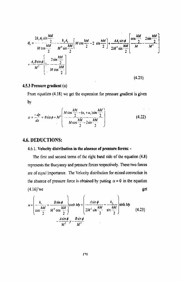
4.5.3 Pressure gradient (a)

From equation (4.18) we get the expression for pressure gradient is given

by

hM Mcos-- - (u , +u2)sin- - - 2

Mcos - -2sin

4.6. DEDUCTIONS:

4.6.1. Velocity distribution in the absence of pressure forces: - The first and second terms of the right hand side of the equation (4.8)

represents the Buoyancy and pressure forces respectively. These two forces

are of equal importance. The Velocity distribution for mixed convection in

the absence of pressure force is obtained by putting a = 0 in the equation

U = I - COS- 'A"- M2cos- "int~]cos~My+l".f 2~~ sin -- - -+]sinhm sin --- (4.23)

4.6.2. Flow between two horizontal plates (i.e. When4 = 0)

4.6.2(a). For the flow of horizontal flat plates, when the two walls are

moving with the velocities U,, U2,

(i) The velocity is given by

UI +u2 u=-------- (UI -4 sjnhMj,t hM

COS~MY------- 2cos

hM 2sin- - cos -

2 2

(4.24)

(ii)The expression for Bulk temperature is given by

hM Mcos- - - ( u , tu,)sin--

(iii) Pressure gradient: a = dx

(4.26)

4.6.2. (b) If one plate is moving and another plate is at stationary:

U ,=0 and U2=U:

The expressions for velocity, Bulk temperature and pressure gradient

are given by

(i) Velocity

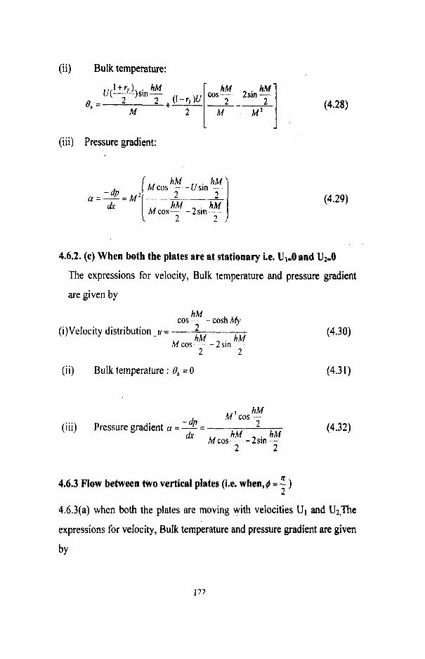
(ii) Bulk temperature:

I + r ) hM U ( - - - ) sin - hM hM

e, = 2 2 + ---- (1 - r , ';[t 2 ~ ~ ~ 1 M 2

(iii) Pressure gradient:

4.6.2. (c) When both the plates are at stationary i.e. UI,O and U2,0

The expressions for velocity, Bulk temperature and pressure gradient

are given by

cos hM - cosh Mv (i)Velocity distribution - u = 2 ---.L

hM hM M c o s -2 s in -

2 2

(ii) Bulk temperature : 8, = 0

hM ~ ' c o s - - - dp (iii) Pressure gradient u = -- = 2

hM hM dr ~ c o s -2sin- - - 2 2

4.6.3 Flow between Wo vertical plates (i.e. when,( = ) 2

4.6.3(a) when both the plates are moving with velocities UI and U2,The

expressions for velocity, Bulk temperature and pressure gradient are given

by

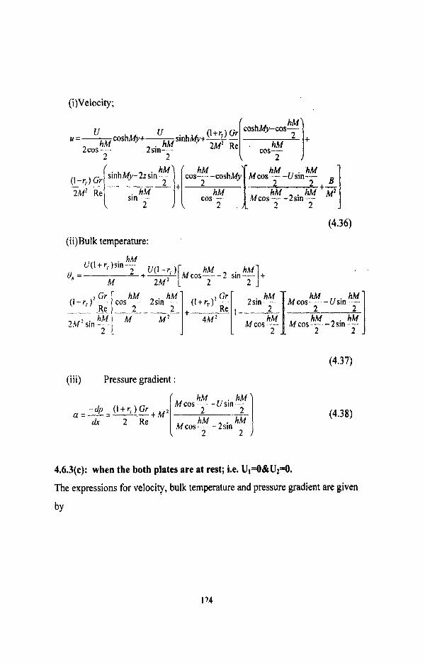
hM (U-U>

coshMz-cos-- u = - ' hM '' coshMy-- sihMytl[ h f 1 +

2 c0s.--- hM

2sin- M2 cos- 2 2

(4.33)

(ii) Bulk temperature:

hM (U, t U,, ( I + rr )sin

6, = 2 - (4 - U , )(I - rT )

M 2MZ

Gr hM ( l - r l ) 2 cos- 2sin---

2 hM M

2 M 2 sin - 2 -

(iii) Pressure gradient:

4.6.3(b) When one plate is at rest and the other plate is moving with

velocity U:'

Then the expressions for velocity, Bulk temperature and pressure

gradient are given by

sinhMy-2z sin

(ii)Bulk temperature:

(iii) Pressure gradient :

4.6.3(c): when the both plates are at rest; i.e. UI=O&Uz4.

The expressions for velocity, bulk temperature and pressure gradient are given

by

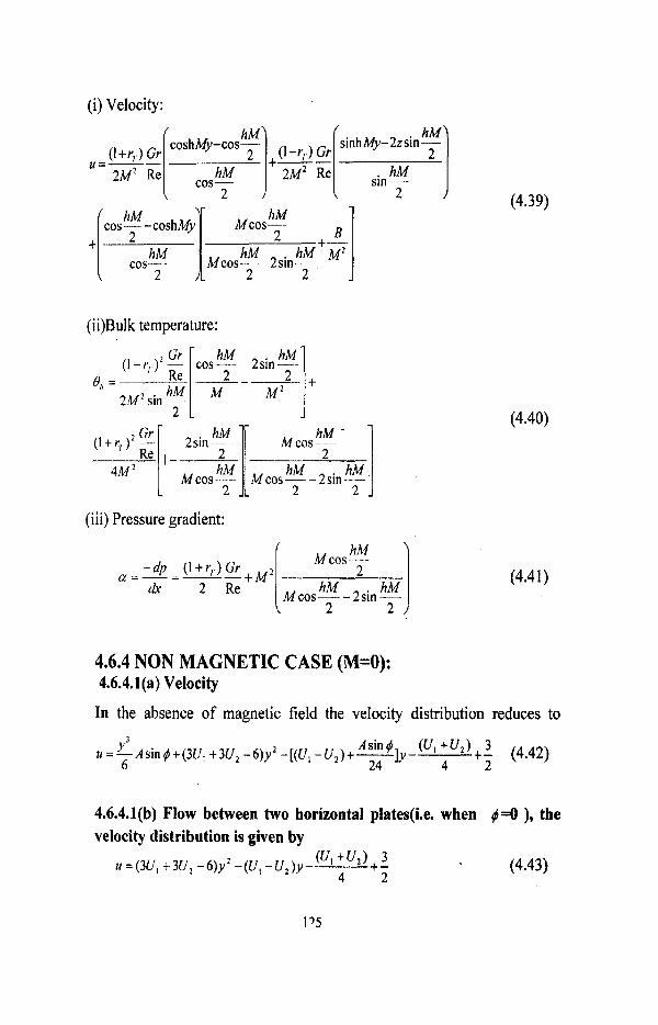
(i) Velocity:

(ii)Bulk temperature:

(iii) Pressure gradient:

4.6.4 NON MAGNETIC CASE (M=O): 4.6.4.1(a) Velocity

In the absence of magnetic field the velocity distribution reduces to

y3 Asin4 (U, t U , ) 3 u =-As in# t (3U , +3U, - 6 ) y 2 - [ (U, - U , ) t - ] y - t- (4.42) 6 24 4 2

4.6.4.1(b) Flow between two horizontal plates(i.e. when (4 ), the velocity distribution is given by

(i) When one plate is at rest and the other plate is moving with velocity U

U 3 i.e. u1=0, U2=U then the Velocity is given by u = (3U -6)$ +@--+- 4 2

(4.44) (ii) When the both plates are at rest; i.e. UI=O&U2=0.then the velocity

distributionk given by

4.6.4.1 (e) .Flow between two perpendicular plrtes(i.e. when ( =?) 2

In the absence of magnetic field the velocity reduces to

lir y3 u=(l-r,)-- (I - r (U, -t.U,) 3 +(3u, +3U, - 6 ) y 2 -[(U, -U,)+-- ]Y- -~-+-

Re 6 24 Re 2

(4.46)

(i) When the lower plate is at rest and the upper plate is moving with

velocity U i.e. UI=O, U2=U then the Velocity is given by

(ii) When the both plates are at rest; j.e. uI=O&u2=0, then the velocity

is given by

4.6.4.2. Bulk temperature for non magnetic case:

The expression for bulk temperature in non magnetic case is obtained by

letting M+O in equation (4.21), we get

These results are in good agreement with Aung and Worku [I 81

4.6.4.2.(a) Flow between two Horizontal p1atesti.e. when 4 = 0)

In the absence of magnetic field and q=O, the expression for bulk

U , + U , I- tr , ) U , - U , temperature is given by 0, = (-

2 ( I - ( 1 - rT (4.50)

(i)When the lower plate is at rest and the upper plate is moving with

velocity U

i.e. U1=O; U2=U then the expression for bulk temperature is

I t ) u Oh = ( - ) U + - ( I - r r )

4 12

(ii)When the both plates are at rest; i.e. UI=O&U2=0

e, = o (4.52)

4.6.4.2(b) Flow between two vertical plates(i.e. When, 4 = E ) 2

In the absence of magnetic field the expression for bulk temperature is

given by

U , t U , I t r , ) U , - U , ( I - r , ) ' Gr 0, = (----- )(----I - (- ) ( I - r,. ) t - -

2 2 12 24 Re

(i) When the lower plate is at rest and the upper plate is moving with

velocity U i.e. UI=O , UPU then the expression for bulk temperature

is

(ii)When the both plates are at rest; i.e. UII=O&U~O then the bulk

( I - r7,12 Gr temperature reduces to 0, = -- (4.55) 24 Re

4.6.4.2(c) Pressure gradient for non magnetic case. Letting M--+O in

equation (4.22) pressure gradient reduces to

4.6.4.3. (a) Flow between two horizontal plates (i.e. when4 = 0)

For non magnetic case and 4 = 0 the expression for pressure gradient is

given by

- $ a = - = 1 2 - 6 ( U , + U , ) (4.57) dx

(i)When the lower plate is at rest and the upper plate is moving with

velocity U i.e. ul=O ,u2=U then the expression for pressure

gradient is given by

(ii)When the both plates are at rest; i.e. U1=O&U2=0 then the expression

for pressure gradient is

4.6.4.3(b) Flow between two vertical plates(i.e. When, 4 = 5 ) 2

!t In the absence of magnetic field and I$ = - the expression for pressure

2

gradient is

(i) When the lower plate is at rest and the upper plate is moving with

velocity U i.e. U1=O ,U2=U then the expression for

pressure gradient is

- dp (1 + r,.) Gr a =- = 12-6u+------ dr 2 Re

(ii) When the both plates are at rest; i.e. U1=O&U2=0 then the

expression for pressure gradient is

These results are in good agreement with G.Krishnaiah et.a1[41]

4.7, RESULTS AND DISCUSSION:

A graphical representation of stream wise velocity profiles for #=dl2

and #=O are shown in figures (1) to (lo), for fixed values of

rT=0,0.25,0.5,0.75,1 .O, UI=1,U2=1, G1-100, 300,500,750 and 1000, and

M=1,2,3,4,5. In figure (1) velocity profiles are shown with the variation of

GrRe. It is noticed that for Gr/Re=100 there is no reversal flow. For

Gr/Re=300 reversal flow is observed near the upper plate, this reversal flow

increases with the increase of GrRe. Near the lower plate y= -1 velocity

increases with the increase of Gr/Re, maximum velocity takes place at y= - 0.35.

In figure (2) velocity profiles are shown for fixed values of rT=0.5,M=l,

UI=l,Uz=land #-1~:/2, It is noticed that velocity increases with the increase of

Gr/Re near the lower plate. Reversal flow is observed for Gr/Re=300,500,750

and 1000 near the upper plate. For Gr/Re=100 no reversal flow is observed. In

figure (3) velocity profiles are shown for fixed values of r d . 2 5 , M=l,

179

#=d2, when the lower plate is at rest and the upper plate is moving with

constant velocityUt=l. It is observed that for Gr/Re=100,300,500 no reversal

flow is found. For Gr/Re=750& 1000 reversal flow is observed near the

moving plate. Near the lower plate which is at rest velocity increases with the

increase of Gr/Re.

In figure (4) velocity profiles are shown for fixed values of rp0.75,

M=l, #=n/2 when both the plates are at rest i.e. UI=O and U2=0. It is observed

that maximum velocity takes place near the centre and the influence of GrRe

is not found on velocity.In figure (5) velocity profiles are displayed with the

variation of magnetic parameter M, for fixed values of r d . 5 , ~ r l ~ e = 2 5 0 ,

#=d2, Ul=l,U.L=I. It is observed that velocity decreases with the increase of

M near the lower plate and the reversal flow is observed near the upper plate,

this reversal flow decreases with the increase of M. In figure (6), velocity

profiles are shown with the variation of M for fixed values of ryO.75,

Gr/Re=500, #=O, U1=O, U2=0. It is noticed that velocity decreases with the

increase of M near the centre of the plates and the reverse action is observed

near the plates. In figure (7) velocity profiles are shown with the variation of

r~ for fixed values of Gr/Re=500, M=2, #=d2, UI=l,Uz=l.It is noticed that

velocity decreases with the increase of rr near the lower plate and the reverse

effect is observed near the upper plate,

In figure (8) velocity profiles are shown with the variation of $ for

fixed values of M . 5 , M=2, GrlRe=500, UI=0,U2=1. It is observed that

velocity increases with the increase of # near the plate which is at rest and

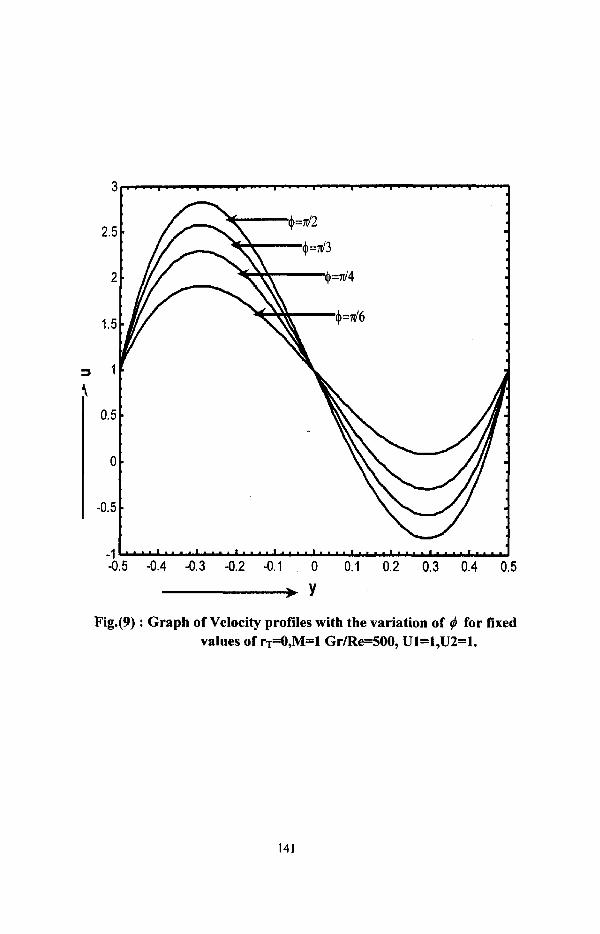
reverse effect is seen near the moving plate.. In figure (9), effect of angle on

velocity is shown for fixed values of r73.0.0, GrBe=500, Ul=l, U2=1. It is

observed that velocity increases with the increase of# near the lower plate and

reverse action takes place near the upper plate. In figure (lo), velocity profiles

are shown for different values of 4 with fixed values of of rfi.25,

Gr/Re=250, U,=0,U2=0.1t is noticed that Velocity increases with the increase

of 4 near the lower plate and the reverse action is observed near the upper

plate, maximum velocity takes place at z= - 0.2.

Graphical representation of Bulk temperature profiles are shown from

figures (1 1) to (17), for fixed values of rT=l.O, M=l, 2, 3, #=d2and 0, U1=l,

Uz=l. In figure (1 1) variations in Bulk temperature are shown for different

values of Magnetic parameter M. It is noticed that Bulk temperature increases

with the increase of M. In figure (12) , Bulk temperature profiles are shown

for M=2,3 and 5, for fixed values of rT=l.O, #=lt/2, UI=0,U2=1. It is noticed

that Bulk temperature increases with the increase of M. In figure (13)

variations in Bulk temperature are shown for different values of M when

r1=1.0, #=n/2and 0, UI=l , Uz=l. It is noticed that the Magnetic parameter M

is not affected the Bulk temperature.

In figure (14) effect of M on Bulk temperature for fixed values of

rT=l.O, #=O, ul=l, u2=1 is shown. It is observed that Bulk temperature

increases with the increase of M. In figure (15) effect of M on Bulk

temperature is shown for r ~ 1 . 0 , #=O,ul=O,u2=1. It is noticed that when one

plate is at rest and another plate is moving with constant velocity 1, Bulk

temperature increases with the increase of M. In figure (16) effect of r~

showed on Bulk temperature for fixed values of d=O, M=2, U1=l,Uz=l. It is

noticed that Bulk temperature decreases with the increase of rT. In figure (17) , Bulk temperature profiles are shown for different values of r~ , it is noticed

that Bulk temperature increase when both the plates are moving with constant

velocity when ( 5 4 2 .

Graphical representation of pressure gradient a is shown fiom figures

(18) to (21) for different values of rd.25,0.5,0.75,1.0, UI=I,U2=1,

M=0.2,0.4,0.5,0,.6,1,5,10. In figure (1 8), effect of Gr/Re on pressure gradient

is shown for different values of r ~ , It is observed that pressure gradient

increases with the increase of r ~ . In figure (19) effect of on pressure

gradient for fixed values of b=O, UI=1,U2=1, M=2shown. It is noticed that

pressure gradient does not change with the variation of rl.. In figure (20),

Pressure gradient profiles are shown for different values of M, for fixed values

of #=0, U1=l,Uz=l and r ~ 1 . 0 . It is observed that pressure gradient increases

with the increase of M. In figure (21) effect of large values of M is shown for

fixed values of $=7c/2, UI=1,U2=1 and r ~ 1 . 0 . It is observed that pressure

gradient increases with the increase of M.

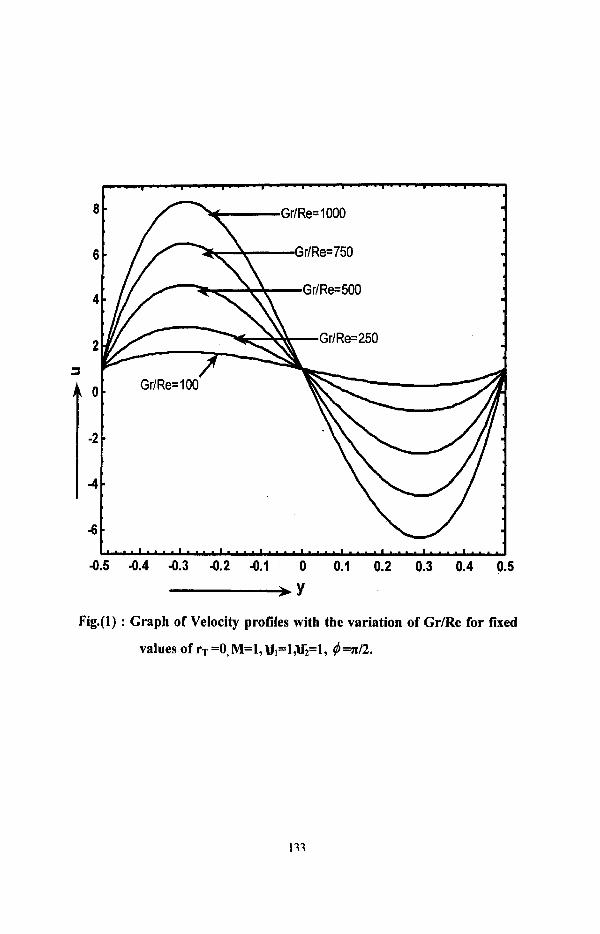
Fig.@) : Graph of Velocity profiles with the variation of GrIRe for fixed

values of r~ =O, M=l,UI=l,l&=l, @=lr/2.

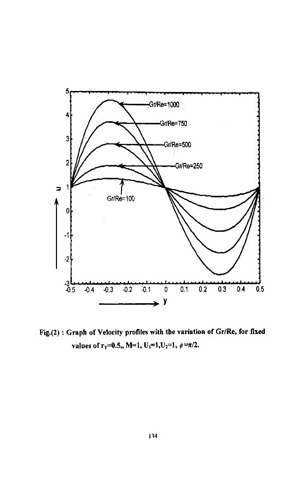
Fig.(2) : Graph of Velocity proliles with the variation of GrIRe, for fixed

values of r . ~ 0 . 5 , , M=l, UI=l,Uz=l, 4 ~ 1 2 .

Fig.(3) : Graph of Velocity profiles with the variation of Gr/Re for fixed values of r.r=0.25,M=1, UI=0,U2=1, 4 =d2.

Fig.(4) : Graph of Velocity profiles with the variation of

Gr/Re for fixed values of r&.75,M=l, U1=0,U2t0, 4 wn.

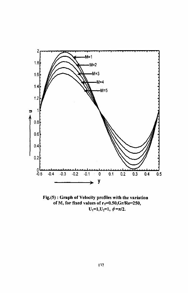
Fig.(J) : Graph of Velocity profiles with the variation of M, for fixed values of rr=0.50,Gr/Re=250,

U,=1,U2=1, 4 312 .

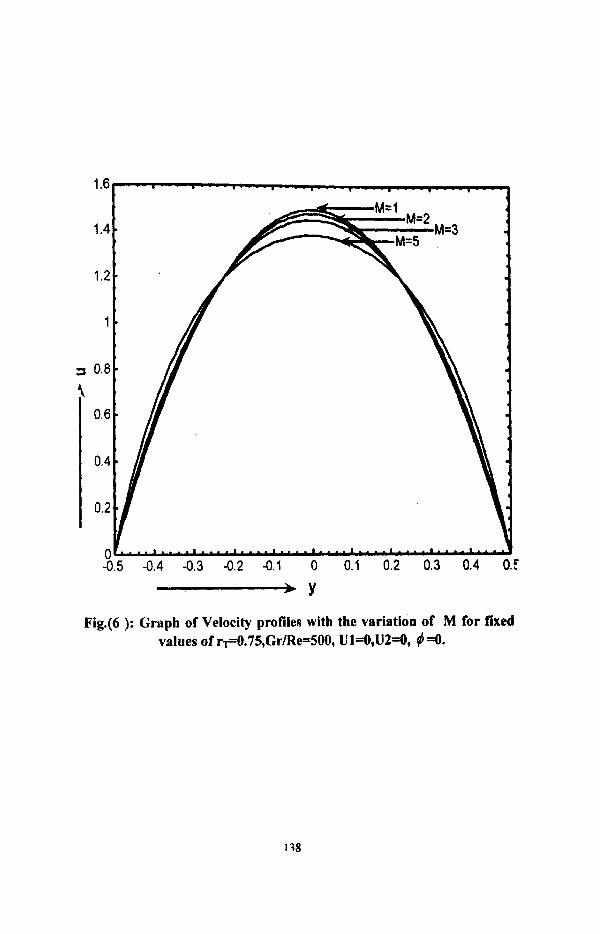
Fig.(6 ): Graph of Velocity profiles with the variation of M for fixed values of r1=0.75,Gr/Re=500, Ul=O,U2=0, (64.

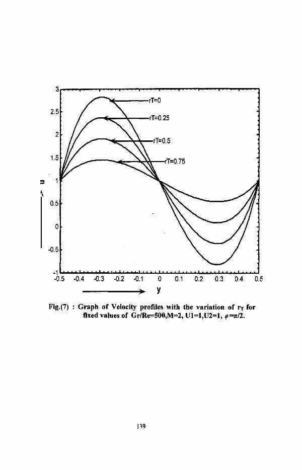
Fig.(7) : Graph of Velocity profiles with the variation of r~ for fixed values of Gr/Re=500,M=2, Ul=l,U2=1, p=le/2.

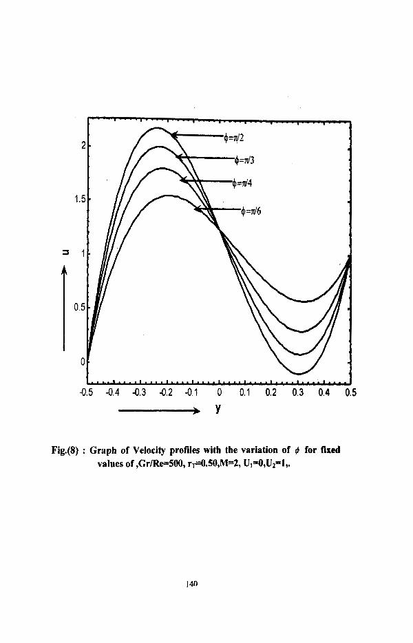
Fig.@) : Graph of Velocity profiles with the variation of # for fixed values of ,Gr/Re=500, rl=0.50,M=2, U14,U2=1,.

3 - - - - m - - - - . - - - - . - - - . - - - - . - - - - . - - - - 1 - - - - 1 - - - - m - - - -

0 .

-0.5 -0.4 -0.3 -0.2 -0.1 0 0.1 0.2 0.3 0.4 0.5

y

Fig.(9) : Graph of Velocity profiles with the variation of # for fixed values of rT=O,M=l Gr/Re=5OO, U1=1,U2=1.

Fig.(lO) : Graph of Velocity profiles with the variation of # for fixed values of rl=0.25,M=1 Gr/Re=ZSO, U l=O,U2=0.

Fig.(ll) : Graph of Bulk Temperature profiles with the variation of M for the fixed values rT=l.O, 4 =z/2 and Ul=l, U2=1.

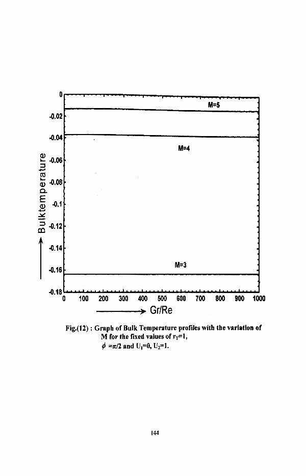
Fig.(l2) : Graph of Bulk Temperature profiles with the variation of M for the fixed values of r p l , 4 3 1 2 and UI=O, U2=l.

Fig.(l3) : Graph of Bulk Temperature profiles with the variation of M, for ry =1.0, q4 4 2 and U I = ~ , U ~ = O .

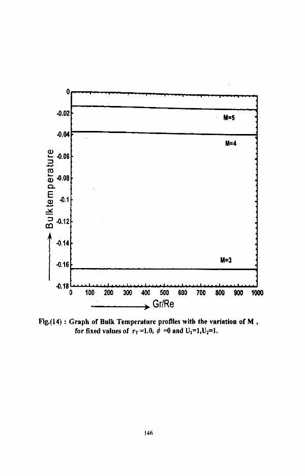
Fig.(l4) : Graph of Bulk Temperature profiles with the variation of M , for fixed values of vr 4.0, 4 4 and UI=1,U2=1.

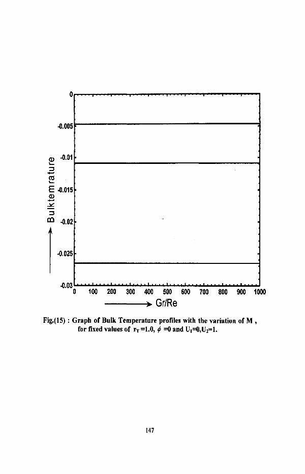
Fig.(lS) : Graph of Bulk Temperature profiles with the variation of M , for fixed values of r~ =LO, # =O and U1=0,Upl.

Fig.(l6) : Graph of Bulk Temperature profiles with the variation of

r~ , For iixed values of 4 =o, U ~ = I , U t l a n d Ms2.

Fig.(l7) : Graph of Bulk Temperature profiles with the variation of r~ , For fixed values of 4 3 1 2 , U1=1,U2=land M=2

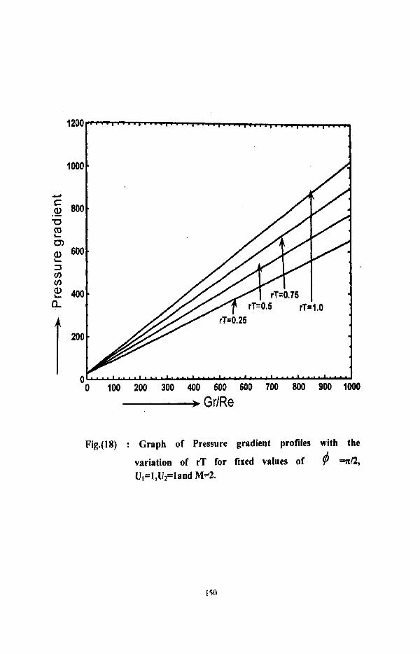
Fig.(lS) : Graph of Pressure gradient profiles with the

variation of rT for fired values of =nn, U,=1,U2=land M=2.

Fig.(l9) : Graph of Pressure gradient profiles with the variation of rT for fixed values of #=O, UI=l,Uz=land M=2

Fig.(ZO) : Graph of Pressure gradient profiles with the

variation of M for fixed values of # 4 ,

Fig.(21) : Graph of Pressure gradient profiles with the

variation of M for fired values of 4 =no , U1=1,U2=land rT=l.O

4.8. CONCLUSIONS:

In this chapter, uniform transverse magnetic field effects due to free and

forced convection of conducting fluid between two parallel flat plates in an

inclined channel is studied. The walls are kept at different uniform

temperature. Expressions for velocity, Bulk temperature and pressure gradient

are obtained for different values of#. The effects of M, GrRe and rr are

studied on the above flow quantities. The following conclusions are made

from this study.

a. Velocity increases with the increase of GrlRe near the lower plate

z= -1 and the reversal flow occurs near the upper plate z= 1.

b. Velocity decreases with the increase of magnetic parameter M at

the centre and the reverse action is observed near the plates.

c. Bulk temperature increase with the increase of M

d. Bulk temperature decreases with the increase of rl. for #=0, and

increase in the case of 4 2 .

e. Pressure gradient increases with the increase of # = d 2 and no

effect of rT is observed in the case of #=0.

f. Pressure gradient increases with the increase of M.

These results are in good agreement with results of G.Krishnaiah et.al

[41], for the case M-rO and Aung and Worku 1261 when ( 4 2 and

M-tO.

4.9. REFERENCES:

1. Aung W: Int.Xof Heat and Mass transfer Vo1.15, 1952. P. 1577-80.

2. Somers E.V: J. Appl. Mech., Vol. 23, 1956, PP.295-301.

3. Rossow, V.J: NACA-TN, 1957, P.3971.

4. Ostorle J-F and F-J Young: XFluid mechanics, 111, part 4, 196 1, 512-

518.

5. Sparrow, E.M & Cess, R.D: XAppl. Mech. Trans. Of ASME, 29, 1,

1961, P181.

6. Bodoia J,R & Osterle J.F: ASME Jof Heat Transfer Vol84, 1962, P.40.

7. Holman J.P: HEAT TRANSFER Mc.Graw hill Book co. Inc, New York.

1 963.

'3. Schlichting H: Boundary layer theory, 6th edition Mc Graw-Hill, New

York. 1965

Q. Beavers G.S and Joseph C.H: ASME J.of Heat Transfer Vo1.30, 1967,

p197.

I0.Mathers W.G., Madden A.J and Piret E. L: India. Engg. Chem., Vo1.49,

1956, PP.961-968.

I I .S.W. Yuan: 1970, Prentice-Hall International, Inc, London.

12,Richardson: LFluid. Mech Vo1.49, 1971, P.327,.

13.Gebhat-t B and Pera L: Int. J. Heat mass transfer, Vol. 14, 1971,

PP.2025-2050.

14.Aung.W: Int.J. Heat Mass tranferl5, 1972, P. 1577-1 580.

1 S.Aung.W, F1echerL.S and Serna5.V: Int.Jof Heat and Mass transfer

VO~. 15, 1972, P. 2293-2308.

16.Callahan G. D and Manner W. J: Transient free convection with mass

transfer on an isothermal verticalflat plate, Vol. 19, 1976, PP 165-174.

17.Michiyochi I., Takahashi 1 and Serizawa A,: Inr. j, Heat muss trans$&,

Vol. 19, 1976, PP. 1021-1029.

18,Riley N. (1976): J. Appl Math. Phys. (ZAMP): Vol. 27, PP. 62 1-63 1

19,Soundelgekar V.M and Wavre P.D: Int. J. Heat mass transfer, Vol. 19,

1977, PP. 1363-1373.

20,Soundalgekar V. M and Ganesan P: Int. .I Eng. Sci., vol. 19, 198 1, PP. .

757-770.

." ' .Acharya B.P and Padhy S: Indian J. ofyure und upplied math.Vol.l4,

1983, P. 83.

ne.Afzal.N, Hussain.T: J. Heat transfer 106, 1984,240-24 1,

f ' .Merkin J.H, A: J, Engg. Math. 19, 1985, 189-20 1.

7-1.M. Necatj Ozisic: HEATTRANSFER A BASIC APPROACI-J, 1885.

?'I.Vijaya Kumar Varma S and Syam Babu M: Indian J-Pure & Appl.

Maths. 16(7), 1985, P.796-806.

26. Aung.W & W0rku.G : ASME J of heat transfer Vo1.108. 1986, PP.

485-488.

r8. R.C.Sachdeva: 1988, Fundamentals of 'ENGINEERING HEAT AND

MASS TMNSFER'N~W age international (p) limited, publishers.

28.Vajravelu K and Nayfeh J: Int. Cornmun, Heat mass transfir, Vol. 19,

1992, PP.70 1-71 0.

19. Watanabe T. and Pop I: Acta. Mech., Vo1.105, 1994, PP. 233-238.

50. Ramalinga Reddy B : Ph.D thesis of 'Magneto hydro dynamics -

someflow problems through porus media '. 1994, S.V.University Tpt.

India.

3 ! .Bejan.A: 1995 Convection Heat transfer, Wiley New York.

32.Elbashbeshy E M. A: Int. JEngg. Sci., Vol. 34, 1997, PP. 515-522.

33.Takhar H. S., Ganesan P., Ekambavahar K and Soundalgekar V M:

Int.J. Numerical methods, Heatfluidflow, Vo1.7, 1997, PP. 280-296.

' :,. R.K. Rajput: 1999, HEAT AND MASS TRANSFER in s. i. Units

S.chand & company LTD

35.Ganesan P and Rani H. P: Int J Ther. Sci., Vo1.39,2000, PP. 265-272.

36. Merkin J.H, 1ngham.D.B: JApp. Math.Phy (ZAMP) 38,2001, 102-1 16.

37.Aboeldahab E M and Elbarbary E M. E: Int J. Eng. Sci., Vol. 39,2001,

PP. 1641-1652.

9. Merkin J.H, Pop.1: Fluid Dynamics ResearchJO, 2002,233-250.

39, Tnti:if,t1g *In"' rae:;s ;.f ' . ' tgr !:yt r ~ ~ ~ f c ; in j'?5;:;iJ7c,w

~ i & " / m - '. 2'-;.;, S.V . Viiiversit-Y, Tpt. India.

40.Chen C. H: Acta. Mech., 2004, Vol. 172, PP. 21 9-235.