mgsc 1205 quantitative methods i
TRANSCRIPT

MGSC 1205
Quantitative Methods I
Ammar Sarhan
Slides Three – LP I: Introduction & Graphical Solution Method

Linear Programming – Introduction
Management decisions in many organizations involve trying to make most effective use of resources. • Machinery, labor, money, time, warehouse space, and raw
materials. These resources can be used to:→Produce products – such as computers, automobiles, or
clothing, … etc. →Provide services – such as package delivery, health services,
or investment decisions.
To solve problems of resource allocation one may use mathematical programming.

Mathematical Programming & LP
Programming refers to setting up and solving a problem mathematically.
Linear programming (LP) is most common type of mathematical programming.
One assumes all relevant input data and parameters are known with certainty in models (deterministic models).
Computers play important in LP.
Properties of a LP Model
All problems seek to maximize or minimize some quantity, usually profit or cost (called objective function).LP models usually include restrictions, or constraints, limit degree to which one can pursue our objective.LP model usually includes a set of non-negativity constraints.
There must be alternative courses of action from which to choose.Objective and constraints in LP problems must be expressed in terms of linear equations or inequalities.

Linear Equations and Inequalities
This is a linear equation:
2A + 5B = 10
This equation is not linear:
2A2 + 5B3 + 3AB = 10
LP uses, in many cases, inequalities like:
A + B ≤ C or A + B ≥ C
An inequality has a ≤ or ≥ sign.

Three Steps of Developing LP Problem
Formulation.Process of translating problem scenario into LP model framework with set of mathematical relationships.
Solution.Mathematical relationships resulting from the formulation process are solved to identify an optimal solution.
Interpretation and Sensitivity Analysis.Problem solver or analyst works with manager to:
• Interpret results and implications of problem solution.• Investigate changes in input parameters and model
variables and impact on problem solution results.

Formulating a LP Problem
A common LP application is a product mix problem.• Two or more products are usually produced using
limited resources – such as personnel, machines, raw materials, and so on.
Profit firm seeks to maximize is based on profit contribution per unit of each product.
Firm would like to determine• How many units of each product it should produce. • Maximize overall profit given its limited resources.

Example: Flair Furniture Company
Company Data and Constraints:Flair Furniture Company produces tables and chairs. Each table sold results in $7 profit, while each chair produced yields $5 profit.Each table requires: 4 hours of carpentry and 2 hours of painting. Each chair requires: 3 hours of carpentry and 1 hour of painting. Available production capacity: 240 hours of carpentry time and 100 hours of painting time. Due to existing inventory of chairs, Flair is to make no more than 60 new chairs.
Flair Furniture’s problem:Determine best possible combination of tables and chairs to manufacture in order to attain maximum profit.

Decision Variables
The decision variables are the elements under control of the model developer and their values determine the solution of the model.
Problem facing Flair is to determine how many chairs and tables to produce to yield maximum profit?
In Flair Furniture problem, there are two unknownvariables.

Objective Function
Objective function states goal of problem• What major objective is to be solved? • Maximize profit!
A LP model must have a single objective function.
In Flair’s problem, total profit may be expressed as:
Profit = ($7 profit per table) × T + ($5 profit per chair) × C
= 7 T + 5 C,where,
T is # tables produced and C is the # chairs produced.T and C are the decision variables.

Constraints
There are 240 carpentry hours available.
There are 100 painting hours available.
The marketing specified chairs limit constraint.
The non-negativity constraints.
Denote conditions that prevent one from selecting any specific subjective value for decision variables.

Constraints
In Flair Furniture’s problem, there are four restrictions on solution:
Restrictions 1 and 2 have to do with available carpentry and painting times, respectively.
Restriction 3 is concerned with upper limit on number of chairs.
A sign restriction is associated with each variable. For any variable, the sign restriction specifies that the variable must be non-negative.
Basic Assumptions of a LP Model
Conditions of certainty exist.
Proportionality in objective function and constraints (1 unit → 3 hours, 3 units → 9 hours).
Additively (total of all activities equals sum of individual activities).
Divisibility assumption that solutions need not necessarily be in whole numbers (integers).

The completed formulation
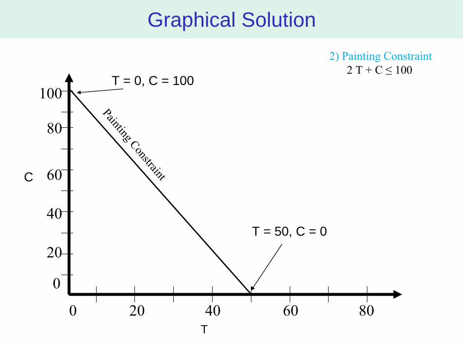
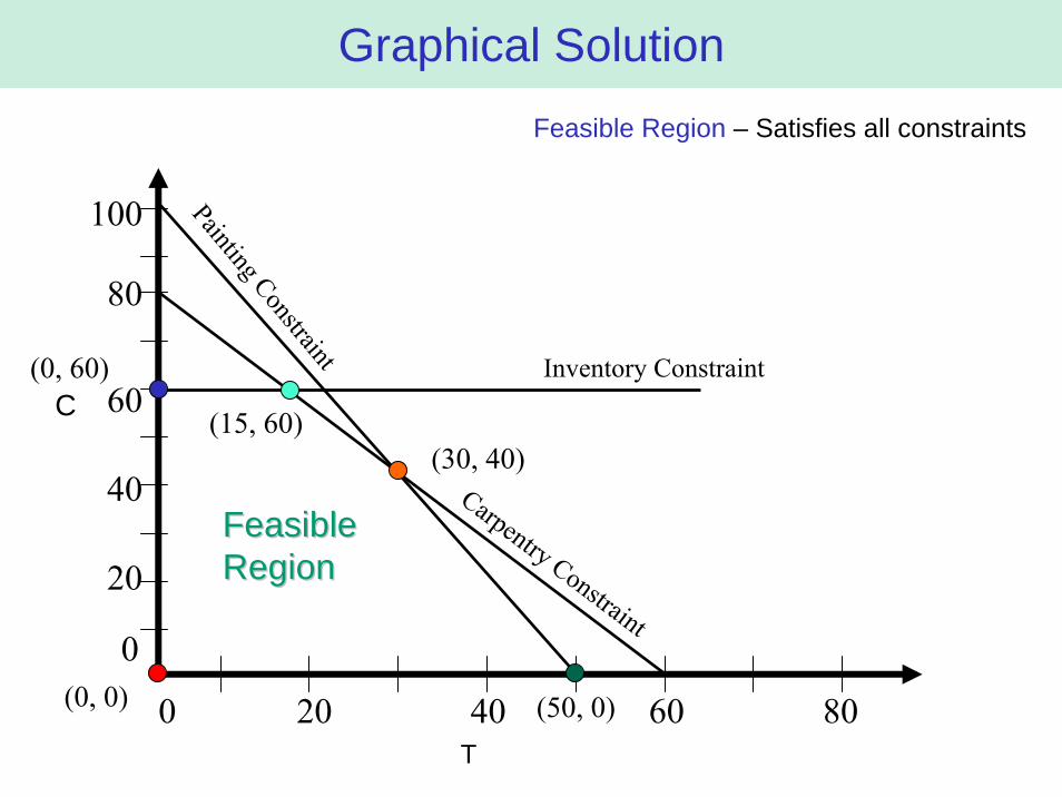
Maximize: P = 7 T + 5 CSubject to (constraints)Carpentry restriction: 4 T + 3 C ≤ 240Painting restriction: 2 T + C ≤ 100Inventory condition: C ≤ 60Non-negativity condition: T ≥ 0, C≥ 0

Graphical Solution
0 20 40 60 80
80
20
40
60
0
100
T
T = 60, C = 0
T = 0, C = 80
Carpentry Constraint
C
1) Carpentry Constraint 4 T + 3 C ≤ 240
Graphical Solution
0 20 40 60 80
80
20
40
60
0
100
T
T = 50, C = 0
T = 0, C = 100
Painting ConstraintC
2) Painting Constraint 2 T + C ≤ 100

Graphical Solution
0 20 40 60 80
80
20
40
60
0
100
T
C
3) Inventory Constraint C ≤ 60
Inventory Constraint
Graphical Solution
0 20 40 60 80
80
20
40
60
0
100
T
Painting Constraint
Carpentry Constraint
C
(30, 40)
Inventory Constraint
(50, 0)(0, 0)
(0, 60)
(15, 60)
Feasible Region – Satisfies all constraints
FeasibleFeasibleRegionRegion

Graphical Solution
0 20 40 60 80
80
20
40
60
0
100
T
C
Optimal solution is the point in the feasible region that produces highest profit There are many possible solution points in the region.Which one is the best?The one yielding highest profit?
FeasibleFeasibleRegionRegion

We can prove that the optimal solution always exists at the intersection of constraints (corner points).• Known as Corner Point Property.
Why not just go directly to the places where the corner points?
Graphical Solution

Corner Point Solution Method
0 20 40 60 80
80
20
40
60
0
100
T
FeasibleFeasibleRegionRegion
C
1
2 3
4
5
Point 1 (T = 0, C = 0)
Point 2 (T = 0, C = 60)
Point 3 (T = 15, C = 60)
Point 4 (T = 30, C = 40)
Point 5 (T = 50, C = 0)

Graphical Solution Procedure
0 20 40 60 80
80
20
40
60
0
100
T
Painting Constraint
Carpentry Constraint
C
Chairs limit constraint
1
2 3
4
5
Point 1 (T = 0, C = 0)
profit = $7(0) + $5(0) = $0
Point 2 (T = 0, C = 60)
profit = $7(0) + $5(60) = $300
Point 3 (T = 15, C = 60)
profit = $7(15) + $5(60) = $405
Point 4 (T = 30, C = 40)
profit = $7(30) + $5(40) = $410
Point 5 (T = 50, C = 0)
profit = $7(50) + $5(0) = $350
FeasibleFeasibleRegionRegion

Example 2
Hours available: 3000 (elect), 2000 (assembly time)Profit / unit: DVD $8, MP3 $10
D = number of DVD players to makeM = number of mp3 players to make
DVD 2 hours electronics work4 hours assembly time
MP3 3 hours electronics work1 hours assembly time

Example
Hours available: 3000 (elect) 2500 (assembly time)Profit / unit: DVD $8, MP3 $10
D = number of DVD players to makeM = number of mp3 players to make
DVD 2 hours electronics work1 hours assembly time
MP3 3 hours electronics work2 hours assembly time
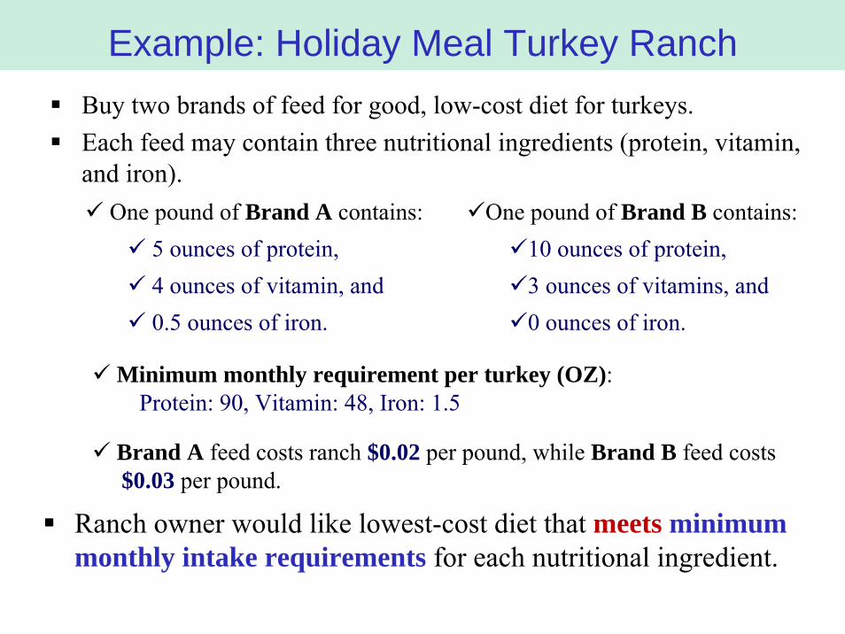
Buy two brands of feed for good, low-cost diet for turkeys. Each feed may contain three nutritional ingredients (protein, vitamin, and iron).
Example: Holiday Meal Turkey Ranch
Ranch owner would like lowest-cost diet that meets minimum monthly intake requirements for each nutritional ingredient.
One pound of Brand A contains:5 ounces of protein, 4 ounces of vitamin, and 0.5 ounces of iron.
Brand A feed costs ranch $0.02 per pound, while Brand B feed costs $0.03 per pound.
One pound of Brand B contains: 10 ounces of protein, 3 ounces of vitamins, and 0 ounces of iron.
Minimum monthly requirement per turkey (OZ):Protein: 90, Vitamin: 48, Iron: 1.5

Example - Fall 2009

Example - Fall 2009