Metric-based anisotropic mesh adaptation for3D acoustic boundary element methods

Stephanie Chaillata,∗, Samuel P. Grothb, Adrien Loseillec

aLaboratoire POEMS UMR CNRS-INRIA-ENSTA, Universite Paris-SaclayENSTA-UMA, 828 Bd des Marechaux, 91762 Palaiseau Cedex, FRANCE

bResearch Laboratory of Electronics, Massachusetts Institute of Technology, Cambridge, MA 02139, USAcGamma 3 Team, INRIA Saclay-Ile de France, 1 Rue Honore d’Estienne d’Orves, 91120 Palaiseau, FRANCE

Abstract

This paper details the extension of a metric-based anisotropic mesh adaptation strategy to the boundary elementmethod (BEM) for problems of 3D acoustic wave propagation. Traditional mesh adaptation strategies for BEMs relyon Galerkin discretizations of the boundary integral equations, and the development of appropriate error indicators.They often require the solution of further integral equations. These methods utilise the error indicators to markelements where the error is above a specified tolerance and then refine these elements. Such an approach cannotlead to anisotropic adaptation regardless of how these elements are refined, since the orientation and shape of currentelements cannot be modified.

On the other hand, the method proposed here is independent of the discretization technique (e.g., collocation,Galerkin). It completely remeshes at each refinement step, altering the shape, size and orientations of elementsaccording to the “optimal” metric based on a numerically recovered Hessian of the boundary solution. The resultingadaptation procedure is truly anisotropic and we show via a variety of numerical examples that it recovers optimalconvergence rates for domains with geometric singularities.

Keywords: Time-harmonic acoustic waves, fast BEMs, Adaptive mesh procedure, Anisotropic mesh.

1. Introduction

We consider the scattering of time-harmonic acoustic waves by three-dimensional obstacles embedded within anunbounded, homogeneous domain. If this problem can be solved with various numerical methods, a natural andpopular approach is to reformulate the problem as a boundary integral equation. The main advantage of such areformulation is its restriction of the computational domain to the boundary of the obstacle and the exact fulfillmentof the outgoing radiation condition. The numerical solution of boundary integral equations is known as the BoundaryElement Method (BEM). Despite the reduction in dimension of the computational domain, the main drawback of theBEM is the fully-populated nature of the system matrix. The cost of BEM simulations is thus prohibitively high whenlarge-scale problems are concerned. Hence there has been a lot of works since the inception of BEMs to reduce itscomputational cost.

If no acceleration technique is used, the storage of such a system is of the order O(N2) where N is the number ofdegrees of freedom on the boundary of the domain. The iterative solution (e.g. with GMRES) is O(NiterN

2) whereNiter is the number of iterations, while the direct solution (e.g. via LU factorizations) is O(N3). In the last decades,different approaches have been proposed to speed up the solution of dense systems. The most known method isprobably the fast multipole method (FMM) proposed by Greengard and Rokhlin [35] which enables a fast evaluationof the matrix-vector product required by the iterative solver. Initially developed for N-body simulations, the FMM hasthen been extended to oscillatory kernels [25, 34]. The method is now widely used in many application fields and hasshown its capabilities in the context of mechanical engineering problems solved with the BEM [16, 45]. An alternativeapproach designed for dense systems is based on the concept of hierarchical matrices (H-matrices) [9]. The principleof H-matrices is to partition the initial dense linear system, and then approximate it into a data-sparse one, by findingsub-blocks in the matrix that can be accurately approximated by low-rank matrices. The efficiency of hierarchicalmatrices relies on the possibility to approximate, under certain conditions, the underlying kernel function by low-rank

∗Corresponding authorEmail addresses: stephanie.chaillat@ensta-paristech.fr (Stephanie Chaillat), samuelpgroth@gmail.com (Samuel P. Groth),

adrien.loseille@inria.fr (Adrien Loseille)

Preprint submitted to Engineering Analysis with Boundary Elements December 4, 2017

matrices. The approach has been shown to be very efficient for asymptotically smooth kernels (e.g. Laplace kernel)and efficient in a pre-asymptotic regime for oscillatory kernels such as Helmholtz or elastodynamic kernels [19].

Mesh adaptation is an additional technique to reduce the computational cost of a numerical method. The principleis to optimize (or at least improve) the positioning of a given number of degrees of freedom on the geometry of theobstacle, in order to yield simulations with superior accuracy compared to those obtained via the use of uniformmeshes. Adaptation is particularly important for scattering obstacles that contain geometric singularities, i.e., edgesand vertices, which lead to a rapid variation of the surface solution near these singularities. For such problems, meshesgraded toward these singularities must be employed in order to yield accurate approximations. Furthermore, for wavescattering problems, we may exploit the directionality of the waves in order to reduce the number of degrees of freedom.The best strategy to achieve these goals is via a so-called “anisotropic” mesh adaptation procedure. If an extensiveliterature is available for volume methods such as Finite Element Methods or Discontinuous Galerkin Methods [1],much less attention has been devoted to BEMs. One possible explanation is the large computational cost of standardBEMs. With the development of fast BEMs such as Fast Multipole accelerated BEMs (FM-BEM) [22] or H-matrixaccelerated BEMs (H-BEM) [12], the capabilities of BEMs are greatly improved such that efficient adaptive meshstrategies are needed not only to optimize further the computational costs but also to certify the numerical results,by assessing that the theoretical convergence order is observed during the computations.

In the BEM community, the majority of the research on mesh adaptation has been confined to isotropic techniqueswith a focus on Laplace equation (see e.g. the exhaustive review [27]) and extensions to Helmholtz equation beingmade only fairly recently [5, 6, 7]. These isotropic techniques are usually based on a posteriori error analysis fromwhich error indicators are derived. An indicator is then used to steer the mesh refinement by systematically markingand refining only elements where the error is above a specified threshold - a process known as Dorfler marking [15].A major challenge is the derivation of local indicators for problems with non-local integral operators [26]. In manyworks (e.g.,[28, 14, 30]) convergence rates for error estimates are proven rigorously. However it is seen that the optimalconvergence rate is not achieved owing to the Dorfler refinement strategy. These techniques do not usually recoverthe optimal convergence rates for 3D problems with anisotropic features [4]. Anisotropic variants of this strategy havebeen considered in [4, 28] however with rectangular elements for cube or cube-like shapes (where all the edges are rightangles). For these shapes they obtain the optimal convergence rate. However for general shapes their approach wouldnot perform as well. The additional drawback of previously published works is the problem-dependent or integralequation-dependent nature of the error estimates. Also, the error analysis of these methods requires a Galerkindiscretization and hence a higher computational cost than, say, a collocation discretization.

The first originality of this work is to extend metric-based anisotropic mesh adaptation (AMA) to BEMs. Metric-based AMA proposed in [38, 39] does not employ a Dorfler marking strategy but rather generates a sequence ofnon-nested meshes with a specified complexity (proportional to the number of vertices or elements). The differentmeshes are defined according to a metric field derived from the evaluation of the linear interpolation error of the(unknown) exact solution on the current mesh. From a theoretical point of view, a continuous metric is derived fromthe Hessian of the exact solution. From a practical point of view, an approximate metric is derived from the numericalsolution only (obtained via the BEM) on a mesh. This approximate Hessian is based on the extension of typical(volumic) derivative recovery operators [46] to the case of numerical boundary solutions. In AMA, the size, shape, andorientation of elements are adjusted simultaneously. The advantages of this approach are that it is ideally suited tosolutions with anisotropic features, it is independent of the underlying PDE and discretization technique (collocation,Galerkin, etc.), and it is inexpensive. The main drawback of this approach is that it relies on assumptions of continuity,which are not true at edges of the obstacle from a theoretical point of view. However, the discrete derivative operatorsdo not need any assumption on the regularity so that a discrete metric can always be computed. Moreover, previousnumerical evidence (e.g.,[2]), in addition to the ones presented in Section 5, suggest that the approach is effectiveregardless of the violation of this assumption. Also, a correspondence between the interpolation and approximationerrors is justified in a simplified context relying on some assumptions on the recovery operator.?? The metric-basedAMA approach, as outlined above, has never been applied to BEMs. The purpose of this paper is to detail and reporton the first application of metric-based AMA to BEMs. Furthermore we address some issues encountered when usingan iterative solver for the FM-BEM on the resulting refined anisotropic meshes. In particular, we present two simpletechniques to reduce the number of GMRES iterations required to achieve convergence when anisotropic elements arecontained in the mesh.

The second originality of this work is the combination of two acceleration techniques, namely metric-basedanisotropic mesh adaptivity (AMA) and FM-BEMs. If no fast BEM is used, the capabilities of anisotropic meshtechniques cannot be demonstrated. The lack of works on adaptive BEMs is mainly due to the high computationalcost of standard BEMs. This original and necessary combination permits to show the performances of the adaptivestrategies.

The outline of the paper is as follows. In Section 2, we recall standard boundary integral equations (BIEs)

2

for scattering problems, its discretization and acceleration with the fast multipole accelerated BEM (FM-BEM). InSection 3, we outline the AMA approach and extend the relevant results from [38, 39] from the case of a 3D volumesolution to a 3D surface solution. In Section 4, we demonstrate the capabilities of the FM-BEM solver and presentresults illustrating the utility of a sequence of meshes to reduce the number of iterations required by the iterative BEMsolver. An array of numerical examples are presented in Section 5 showing the recovery of the optimal convergencerate for scatterers with geometric singularities.

2. Standard and accelerated boundary element methods

2.1. Boundary integral equations for 3D Helmholtz equation

Consider a closed bounded domain Ω ⊂ R2 with boundary Γ and let Ω+ := R3\Ω denote the exterior scatteringdomain. Suppose that we have an incident plane wave ui with wavenumber k := 2π/λ (where λ is the wavelength)and direction d; this may be written as

ui(x) = eikd·x, x ∈ R3.

ui is scattered by Ω leading to a scattered field us which, when combined with ui, gives the total field u in Ω+. Thistotal field is such that

∇2u+ k2u = 0 in Ω+. (1)

In this work, we consider only sound soft boundary conditions (BC)

u = 0 on Γ. (2)

The adaptation method presented later is nevertheless more general, and can be applied to problems with Neumann,mixed or transmission boundary conditions. Furthermore, we require that us = u − ui satisfies the Sommerfeldradiation condition

limr→∞

(∂us

∂r− ikus

)= 0,

where r = |x|.The first main difficulty arising in the numerical solution to this exterior boundary value problem is related to the

unboundedness of the computational domain Ω+. Integral equation based methods are one of the possible tools toovercome this issue. The approach is based on the potential theory [23]. For any positive real number k, let

Φ(x,y) =eik|x−y|

4π|x− y|

be the fundamental solution of the 3D Helmholtz equation. The single-layer potential operator is defined by

Sφ(x) :=

∫Γ

Φ(x,y)φ(y)ds(y).

The trace of the single-layer potential is given by applying the exterior Dirichlet trace to S such that we have

(Sφ)|Γ = Sφ.

The boundary integral operator S is defined, for x ∈ Γ by

Sφ(x) :=

∫Γ

Φ(x,y)φ(y)ds(y).

There exist various possible integral equations to obtain the Cauchy data. For the numerical examples considered inSection 5, we use the simplest choice for the sound-soft problems. We employ the Dirichlet EFIE formulation usingonly the single-layer operator

Sq = −ui. (3)

The solution of the integral equation (3) is the trace of q = − ∂u∂n on the boundary of the domain. The value in the

domain is then obtained by using the following boundary integral representation

us(x) = Sq(x), x ∈ Ω+. (4)

3

When the problem at hand does not have a thickness, we require a slight modification of the BIE for these problemssince here the unknown is the jump in ∂u/∂n across the surface, rather than ∂u/∂n itself. We denote this jump by[∂u∂n

]. So the BIE to solve is [44]:

−ui(x) =

∫Γ

Φk(x,y)

[∂u

∂n

](y)ds(y), x ∈ Γ. (5)

It is known [42] that the integral equation (3) is not uniquely solvable for all wavenumbers k. Hence, in practice,it is often preferable to employ so-called “combined” formulations, such as the combined integral formulations [20],which are uniquely solvable for all k but are more computationally expensive. However, for the purpose of the presentpaper, the choice of integral equation is not particularly important since our focus is to demonstrate the applicationof AMA to BEMs. Thus we choose to employ the simplest BIE formulation in order to keep the computational costat a minimum.

2.2. BEM discretization and Fast multipole accelerated BEM for the 3D Helmholtz equation

The main ingredients of BEMs are a transposition of the concepts developed for the Finite Element Method [11].First, the numerical solution of the boundary integral equation (3) is based on a discretization of the surface Γ intoNE isoparametric boundary elements of order one, i.e. three-node triangular elements. Each physical element Ee onthe approximate boundary is mapped onto a reference element ∆e via an affine mapping

ξ ∈ ∆e → y(ξ) ∈ Ee, 1 ≤ e ≤ Ne.∆e is the reference triangle in the (ξ1, ξ2)-plane. The N interpolation points y1, . . . ,yN are chosen as the vertices of themesh. Each unknown field q is approximated with globally continuous, piecewise-linear shape functions (vi(y))1≤i≤N :vi(yj) = δij for 1 ≤ i, j ≤ N . A boundary element Ee contains exactly 3 interpolation nodes (yek)1≤k≤3 associatedwith 3 basis functions (vek)1≤k≤3. These basis functions are related to the canonical basis (vk)1≤k≤3 defined on thereference element ∆e by vek(y(ξ)) = vk(ξ). Each unknown field is approximated on the element Ee by

q(y) ≈3∑k=1

qkvek(y),

where qk denotes the approximation of the nodal value of q(yk). To discretize the boundary integral equation (3), weconsider the collocation approach. It consists in enforcing the equation at a finite number of collocation points x. Tohave a solvable discrete problem, one has to choose N collocation points. The N approximation nodes thus definedalso serve as collocation points, i.e. (xi)1≤i≤N = (yj)1≤j≤N . This discretization process transforms (3) into a squarecomplex-valued linear system of size N of the form

Aq = b, (6)

where the (N)-vector q collects the degrees of freedom (DOFs) while the (N)-vector b arises from the imposedincident wave field. Assembling the matrix A classically [11] requires the computation of all element integrals for eachcollocation point, thus requiring a computational time of order O(N2). To lower this O(N2) complexity, which isunacceptable for large BEM models, fast BEM solution techniques such as the Fast Multipole Method (FMM) mustbe employed.

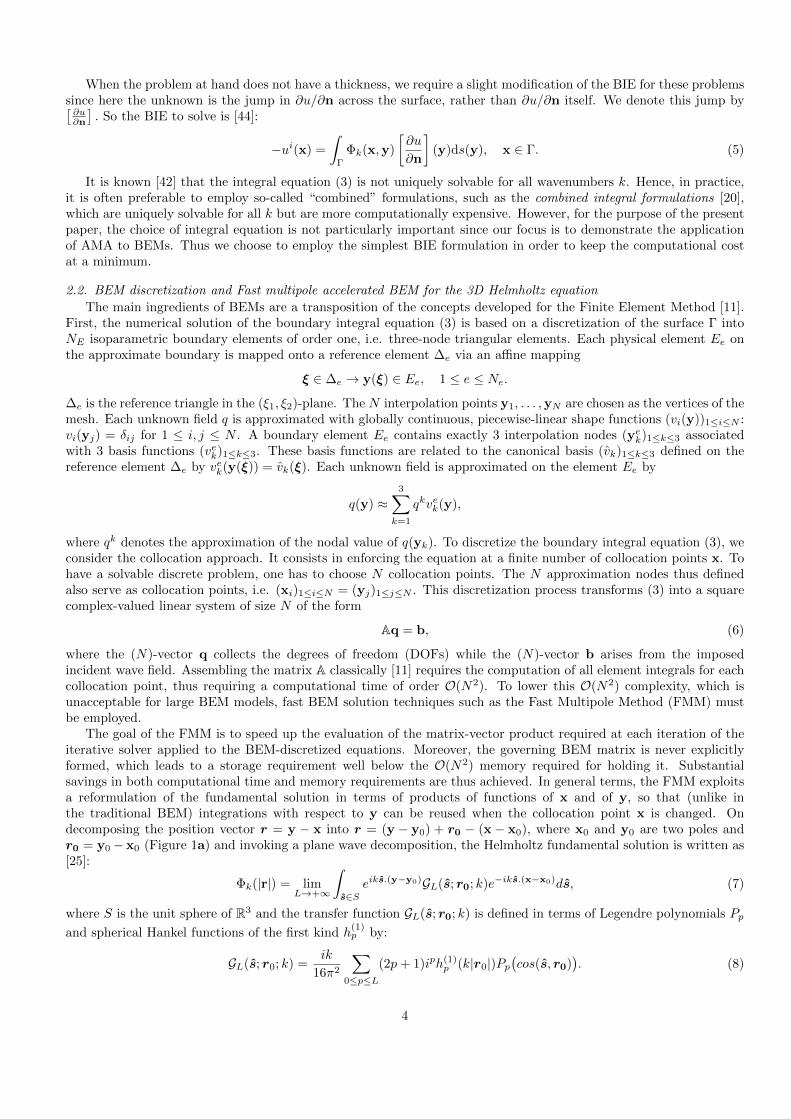
The goal of the FMM is to speed up the evaluation of the matrix-vector product required at each iteration of theiterative solver applied to the BEM-discretized equations. Moreover, the governing BEM matrix is never explicitlyformed, which leads to a storage requirement well below the O(N2) memory required for holding it. Substantialsavings in both computational time and memory requirements are thus achieved. In general terms, the FMM exploitsa reformulation of the fundamental solution in terms of products of functions of x and of y, so that (unlike inthe traditional BEM) integrations with respect to y can be reused when the collocation point x is changed. Ondecomposing the position vector r = y − x into r = (y − y0) + r0 − (x− x0), where x0 and y0 are two poles andr0 = y0−x0 (Figure 1a) and invoking a plane wave decomposition, the Helmholtz fundamental solution is written as[25]:

Φk(|r|) = limL→+∞

∫s∈S

eiks.(y−y0)GL(s; r0; k)e−iks.(x−x0)ds, (7)

where S is the unit sphere of R3 and the transfer function GL(s; r0; k) is defined in terms of Legendre polynomials Pp

and spherical Hankel functions of the first kind h(1)p by:

GL(s; r0; k) =ik

16π2

∑0≤p≤L

(2p+ 1)iph(1)p (k|r0|)Pp

(cos(s, r0)

). (8)

4

x

x0 y0

y

r r0

d

∂Ω

(a) (b)

Figure 1: Fast Multipole Method: (a)Decomposition of the position vector and (b) 3D cubic grid embedding the boundary.

It can be shown that Expression (7) is valid only for well-separated sets of collocation and integration pointsclustered around poles x0 and y0.

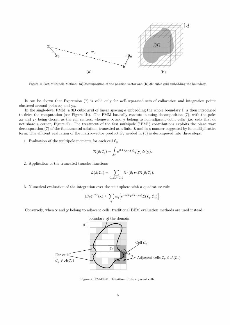
In the single-level FMM, a 3D cubic grid of linear spacing d embedding the whole boundary Γ is then introducedto drive the computation (see Figure 1b). The FMM basically consists in using decomposition (7), with the polesx0 and y0 being chosen as the cell centers, whenever x and y belong to non-adjacent cubic cells (i.e. cells that donot share a corner, Figure 2). The treatment of the fast multipole (”FM”) contributions exploits the plane wavedecomposition (7) of the fundamental solution, truncated at a finite L and in a manner suggested by its multiplicativeform. The efficient evaluation of the matrix-vector product Sq needed in (3) is decomposed into three steps:

1. Evaluation of the multipole moments for each cell Cy

R(s; Cy) =

∫Γ

eiks.(y−y0)q(y)ds(y).

2. Application of the truncated transfer functions

L(s; Cx) =∑

Cy /∈A(Cx)

GL(s; r0)R(s; Cy).

3. Numerical evaluation of the integration over the unit sphere with a quadrature rule

(Sq)FM (x) ≈∑q

wq

[e−iksq.(x−x0)L(sq; Cx)

].

Conversely, when x and y belong to adjacent cells, traditional BEM evaluation methods are used instead.

Cell Cx

Adjacent cells Cy ∈ A(Cx)Far cells

Cy /∈ A(Cx)

Ω

boundary of the domain

d

Figure 2: FM-BEM: Definition of the adjacent cells.

5

To improve further the computational efficiency of the FM-BEM, standard (i.e. non-FMM) calculations must beconfined to the smallest possible spatial regions while retaining the advantage of clustering the computation of influenceterms into non-adjacent large groups whenever possible. This is achieved by recursively subdividing cubic cells intoeight smaller cubic cells. New pairs of non-adjacent smaller cells, to which plane wave expansions are applicable, arethus obtained from the subdivision of pairs of adjacent cells. The cell-subdivision approach is systematized by meansof an octree structure of cells. At each level `, the linear cell size is denoted d`. The level ` = 0, composed of onlyone cubic cell containing the whole surface Γ, is the tree root. The subdivision process is further repeated until the

finest level ` = ¯, implicitly defined by a preset subdivision-stopping criterion (d¯ ≥ dmin), is reached. Level-¯ cells

are usually termed leaf cells. This is the essence of the multi-level FMM, whose theoretical complexity is O(N logN)per GMRES iteration both for computational time and memory requirements.

2.3. Regularity of the boundary data

A standard rule of thumb for wave approximation problems is that between 6 and 10 degrees of freedom perwavelength are required to achieve “engineering accuracy” with numerical methods [41]. The most popular way todistribute these degrees of freedom is over a uniform mesh of the surface. However, for calculations involving scattererswith edges, it is well known that this accuracy can be severely diminished if uniform meshes are employed [36].Furthermore, the convergence of BEMs for these problems will be suboptimal. This is due to the low regularity of theboundary data at edges. In particular, at an edge, we expect the acoustic pressure u, to behave as [36]

u ∼ r πα as r → 0, (9)

where r is the distance from the edge, and α is the exterior angle. Hence the flow velocity will behave as

∂u

∂n∼ r πα−1 as r → 0. (10)

At vertices where two or more edges meet, the singularities in u and ∂u/∂n are even more severe and do not havesimple expressions such as (9) and (10) (see, e.g., [8]).

In order to accurately approximate the solutions of such scattering problems and recover the optimal convergenceorder, the mesh must be appropriately refined towards the edges. We note that the optimal order of convergence forP1 discretizations is O(N−1) where N is the number of degrees of freedom. Optimal a priori refinement strategies canbe devised via a consideration of the polynomial interpolation of functions with the appropriate singularities [3, 33].However, for complicated scattering geometries with vertices, designing an optimal mesh is challenging and ofteninfeasible. Hence adaptive meshing strategies have proven popular. In the next section we describe the adaptivestrategy employed here.

3. Metric-based anisotropic mesh adaptation

In this Section, we review the main existing results of the metric-based anisotropic mesh adaptation procedureand derive new estimates for the case of 3D surface solutions. Further details on the approach derivation for volumesolutions and examples of application can be found in [38, 39], or in [2] for a comprehensive overview.

The goal of mesh adaptation is to find the optimal mesh that permits to minimize the approximation error, due tothe use of a BEM solver in our context. To date, most mesh adaptation approaches for BEMs rely explicitly on thelocal error estimation of the boundary approximation to drive the adaptation procedure. The derivation of appropriatelocal error estimators is a significant challenge owing to the non-locality of boundary integral operators. This difficultyis the main reason why adaptivity for BEMs is a much less well-explored research topic in comparison to adaptivityfor FEMs where the relevant operators are local differential operators.

The metric-based adaptivity method employed in this paper is also linked to the error in the surface approximationbut in a much less explicit way. In addition, it is not linked to the underlying boundary integral operators. Rather,our method is connected to the linear interpolation error of the (unknown) exact solution on the mesh (interpolationwith higher order functions has not yet been considered) with a specified norm. Then, given a number of degreesof freedom, meshes which minimise this interpolation error are designed in an anisotropic setting. Via argumentsrelating the BEM approximation error to this interpolation error, such meshes are seen to be close to optimal for BEMsolutions. Many authors have considered such a technique, e.g., [21]. However it is the first time it is used in thecontext of BEMs. In what follows, we focus on the description of metric-based mesh adaptation in the BEM context,i.e., we assume that the solution is only provided on the boundary Γ.

6

3.1. Metric-based mesh generation

A convenient framework to generate anisotropic meshes is to use Riemannian metric spaces. A Riemannian metricspace is defined by a metric tensor M(x), i.e., is a smoothly varying function of the physical variable x. In thecontext of anisotropic mesh generation, each mesh vertex x has an assigned value M(x) which dictates the size andorientation of adjacent elements. By generating a unit mesh in the corresponding Riemannian metric space, we obtainan anisotropic mesh refined according to the metricM. This is the fundamental idea of metric-based mesh adaptationas introduced in [31].

A surface mesh HN , associated with a Riemannian metric space M = (M(x))x∈Γ (where M is the metric tensor)is a triangulation of the surface Γ. A triangle K, which is defined by its edges ei3i=1, is unit with respect to M ifthe length of each edge is unit in this metric, i.e., if

||ei||M :=√

eTiMei = 1, for i = 1, 2, 3. (11)

If the three edges of K are of unit length with respect to the metric tensor M, then the area of K computed in theRiemannian (|K|M) or Euclidean (|K|) space are

p3

2

1

|K|M =

√3

4, and |K| =

√3

4det(M−1/2).

The existence of a conforming unit mesh in which each triangle is unit with respect to a given Riemannian metricspace is not guaranteed in general. Hence the objective of seeking a unit mesh must be relaxed somewhat. We seeka quasi-unit mesh with respect to M, which is a mesh composed of quasi-unit triangles. A triangle K is quasi-unitwith respect to M if

1√2≤ ||ei||M ≤

√2, for i = 1, 2, 3, and |K|M =

√3

4. (12)

Using the above notion of a quasi-unit mesh, the generation of anisotropic meshes is simplified. The mesh generatoris only required to generate a quasi-unit mesh in the prescribed Riemannian metric space, and this is shown to bealways possible [31]. The generated mesh is adapted and anisotropic in the Euclidean space.

Once the metric-space setting established, the next Section presents the generation of the appropriate metrictensor to reduce the approximation error. The principle is to minimize the error coming from linear interpolation ofthe (unknown) exact solution. Since the linear interpolation error involves the Hessian of the solution, a metric-tensorbased on this Hessian is derived.

3.2. Dealing with a surface solution: Surface projection operators

AMA theory has been developed for 2D and 3D volume solutions. In the BEM context, we cannot applied directlythe results as even though we work in 3D, we only have the solution on a surface. In particular, we cannot recoverthe full Hessian of the numerical solution but only its trace on the boundary. In a similar way, only the trace on theboundary of the interpolation error can be estimated. It is then necessary to introduce some mapping in order to onlytake into account the surface component of each value of interest.

t2

t1a

n

Figure 3: To extend the concept of metric-based error estimates, we introduce a surface projection on the local tangent plane.

In what follows, we assume that the boundary Γ of the computational domain is smooth (at least by patches). Wethen have a local Frenet frame (n, t1, t2) defined at each point, where n is the normal to the surface and, t1 and t2 are

7

orthonormal directions in the tangent plane (see Fig. 3). Given a 3D quadratic form Q(a) (for example the Hessian ora metric) evaluated at a surface point a provided with a local Frenet frame (n, t1, t2), we want to remove its variationwith respect to the normal component (to reuse tools already defined for volume solutions). To this aim, we definethe tangent plane projection Ps (which gives Q(a) in the local tangent plane):

Ps(Q(a)) =

(tt1Q t1

tt1Q t2tt1Q t2

tt2Q t2

).

On the other hand, Q(a) in the 3D frame is given by:

Q(a) = t(n t1 t2)

(Ps(Q(a)) 0

0 tnQ(a)n

)(n t1 t2).

This tangent plane mapping is used to comply with the BEM context in which the solution is known only on thesurface. It is clear that the variation of the solution along the normal direction cannot be estimated.

Once the metric-space setting established, the next Section presents the generation of the appropriate metrictensor to reduce the approximation error. The principle is to minimize the error coming from linear interpolation ofthe (unknown) exact solution.

3.3. Controlling the linear interpolation error in the tangent plane

We suppose that the solution u is sufficiently smooth to possess a second order Taylor approximation. For 3Dvolume solutions, the quadratic approximation uq of u is given by its truncated Taylor expansion

u(x) ≈ uq(x) := u(a) + t∇u(a)(x− a) +1

2t(x− a)H(a)(x− a),

where H is a symmetric matrix representing the Hessian of u, that is,

Hij(x) =∂2u(x)

∂xi∂xj, i, j = 1, 2, 3. (13)

When working with 3D surface solutions, we need to introduce the local system of coordinates in the tangent planecentered at a (i.e., the new variable X), and us the projection of u in the tangent plane. Then, we consider thequadratic approximation uqs of us, i.e.,

us(X) ≈ uqs(X) := us(0) + t∇us(0)X +1

2tXPs(H(a))X. (14)

Note that to build this theory it is assumed that the solution is smooth (twice differentiable). It is well knownthat this is not the case for obstacles with edges and vertices [40]. At these geometric singularities, the solution andits derivatives may be discontinuous. However, away from these points the solution should be smooth. In practice,it has been observed that even though this assumption is violated, adaptation methods based on the control of thelinear interpolation error are still very effective for volume solutions [39]. The explanation is that these assumptionsare only needed to state the optimality of the method. The practical technic to recover the Hessian only relies on theuse of the numerical solution without any required regularity.

We now have all the tools to derive an estimation of the interpolation error. We follow the same ideas than in [38].We note Πh the discrete linear interpolation operator such that Πhus is the linear interpolant of us on the mesh HN .The starting point is to show that the interpolation error in L1 norm of a 3D surface solution us on a triangularelement K is

||us −Πhus||L1(K) =|K|24

3∑i=1

tei Ps(H) ei, (15)

where the ei are the edges of the triangle K provided in the local tangential frame. The proof is based on theevaluation of the point-wise interpolation error within the element, i.e. e(x) = (us − Πhus)(x) for x ∈ K. It onlyuses the mapping onto the reference element and the knowledge that the solution is a quadratic function. This erroris then integrated over the element.Proof: The reference element Kref is defined by its three vertices:

x1 = t(0, 0), x2 = t(1, 0), x3 = t(0, 1).

8

The mapping onto the current element K is given by:

x = v1 +BK x with BK = [x2 − x1,x3 − x1] = [e1, e2], x ∈ K, x ∈ Kref ,

where v1 is c’est plutot x1? and we have introduced the edges: e1 = x2−x1, e2 = x3−x1 and e3 = x3−x2. Thequadratic function us reads in the frame of Kref :

us(x(x)) =1

2tx1 Ps(H)x1 +

1

2tx1 Ps(H)BK x +

1

2tx tBK Ps(H)x1 +

1

2tx tBK Ps(H)BK x.

As we consider a linear interpolation, the linear and constant terms of us(x(x)) are exactly interpolated such thatonly quadratic terms are kept. We introduce us(x) = 1

2tx tBK Ps(H)BK x, then it comes:

e(x) = (us −Πhus)(x) = (us −Πhus)(x).

We rewrite us in a matrix form:

us(x(x)) =1

2t

(xy

)[te1Ps(H)e1

te1Ps(H)e2te2Ps(H)e1

te2Ps(H)e2

](xy

),

and then us in Kref reads:

us(x(x)) =1

2

((te1Ps(H)e1) x2 + (te2Ps(H)e2) y2 + 2(te1Ps(H)e2) xy

).

us is now linearly interpolated on Kref . Its linear interpolate Πhus(x) writes ax + by + c, where the coefficients(a, b, c) ∈ R3 satisfy the following linear system ensuring Πhu(vi) = u(vi) for all i ∈ [1, 3], with vi the vertex i c’estplutot xi? :

Πhus(v1) = us(x(0, 0)) = 0 = c,

Πhus(v2) = us(x(1, 0)) = 12 (te1Ps(H)e1) = a,

Πhus(v3) = us(x(0, 1)) = 12 (te2Ps(H)e2) = b.

The solution of the previous linear system gives the final expression of Πhus:

Πhus(x(x)) =1

2

[(te1Ps(H)e1) x+ (te2Ps(H)e2) y

].

The exact point-wise interpolation error e(x) is then given by:

e(x(x)) =1

2[ (te1Ps(H)e1) (x2 − x) + (te2Ps(H)e2) (y2 − y) + 2 (te1Ps(H)e2) xy ].

Classically, for every function F , its integration over K can be computed through its expression in Kref :∫K

F (x) dxdy =

∫Kref

F (x(x)) |det(BK)|dxdy = 2|K|∫Kref

F (x(x)) dxdy.

Consequently, the interpolation error in L1 norm, evaluated by a direct integration of |e(x)|, is given by

‖us −Πhus‖L1(K) =2|K|24

∣∣te1 Ps(H) e2 − te1 Ps(H) e1 − te2 Ps(H) e2

∣∣.The crossed term can be expressed only in terms of ei Ps(H) ei for i = 1, .., 3 by remarking that e1 − e2 + e3 = 0 itfollows

2te1 Ps(H) e2 = te1 Ps(H) e1 + te2 Ps(H) e2 − te3 Ps(H) e3,

and we deduce:

2∣∣te1 Ps(H) e2 − (te1 Ps(H) e1 + te2 Ps(H) e2)

∣∣ =

∣∣∣∣∣3∑i=1

tei Ps(H) ei

∣∣∣∣∣ .If us is hyperbolic, the inequality 1

2 |xPs(H)x| ≤ 12x |Ps(H)|x is used to conclude the proof in the general case. ca

veut dire quoi??

9

We consider now all elements K which are unit with respect to the metric Ps(M). The next step consists inshowing that

3∑i=1

tei Ps(H) ei =3

2trace(Ps(M)−

12 Ps(H)Ps(M)−

12 ).

Proof: We consider first the simple case where Ps(H) = I2 and Ps(M) = I2. The regular triangle K0 = (x1,x2,x3)unit for I2 is defined by the vertices:

x1 = (0, 0) , x2 = (1, 0) , x3 =

(1

2,

√3

2

).

We first show the following preliminary result: For all lines (D) passing through one of the vertices of K0, the sum ofthe square lengths of the edges projected on (D) is invariant.

Without loss of generality, we assume that (D) passes through the vertex x1 of K0. If (D) is defined by the vector

n = (cos(v), sin(v)) ,

with v ∈ R, then the length of the three edges of K0 projected on (D) are given by:

a = e1 .n = cos(v), b = e2 .n =1

2cos(v) +

√3

2sin(v), c = e3 .n =

−1

2cos(v) +

√3

2sin(v).

Such that a2 + b2 + c2 = 3/2. When Ps(M) is different from I2, we use Ps(M−12 ) that maps the unit ball of I2

onto the unit ball of Ps(M). (D) is now directed by one of the eigenvectors of Ps(M), e.g. vj , and which is passingthrough x1. The lengths a, b and c are thus multiplied by hj , i.e. the size prescribed by Ps(M) in the direction vj .Consequently, the square length of the edges projected on (D) are multiplied by h2

j . It comes using the preliminaryresult:

3∑i=1

(tei vj)2 =

3

2h2j .

Considering this relation for the two principal directions of Ps(M), we obtain:

3∑i=1

‖ei‖22 =

2∑j=1

3∑i=1

(tei vj)2 =

3

2

(h2

1 + h22

)=

3

2trace(Ps(M)−1). (16)

We now consider the general case where a symmetric matrix Ps(H) is involved in the estimation instead ofPs(H) = I2. Ps(H) being symmetric, it has two real eigenvalues (µi)i=1,2 along the principal directions (ui)i=1,2. If Kis a regular triangle with edges (ei)i=1,3, according to the preliminary result, the sum of the projected square lengthof edges (ei)i=1,3 on each principal direction uj is equal to 3/2. We deduce:

µj

3∑i=1

(tei uj)2 =

3

2µj , for j ∈ [1, 2] and

2∑j=1

3∑i=1

µj (tei uj)2 =

3

2(µ1 + µ2).

The previous equality reads:3∑i=1

tei Ps(H)ei =3

2trace(Ps(H)).

We deduce the general case by taking Ps(M)−12 Ps(H)Ps(M)−

12 as symmetric matrix. In that case, each edge ei of

the regular triangle is mapped on ei = Ps(M)−12 ei. The new triangle defined by edges (ei)i=1,3 is unit with respect

to Ps(M). This concludes the proof.

Using that |K| =√

34 det(Ps(M)−1/2), the interpolation error (15) is finally expressed for a 3D surface solution by:

||us −Πhus||L1(K) =

√3

64det(Ps(M)−

12 ) trace(Ps(M)−

12 Ps(H)Ps(M)−

12 ). (17)

The computation of the discrete interpolation error on a unit mesh H with respect to M = (Ps(M)(x))x∈Γ thenreduces to

||us −Πhus||L1(Γh) =∑K∈H

||us −Πhus||L1(K).

10

Importantly, (17) implies that the interpolation error does not depend on the element shape, i.e., on the mesh generator.The metric alone contains enough information to describe completely the linear interpolation error in L1 norm. Inaddition, this interpolation error is expressed with continuous quantities only. It is thus possible to define a continuouslinear interpolation function πPs(M), independent from the discrete mesh, such that

|us − πPs(M)us|(a) = 2||us −Πhus||L1(K)

|K| =1

8trace(Ps(M)−

12 Ps(H)Ps(M)−

12 ). (18)

Finally, the continuous interpolation error calculated on the continuous mesh M is given by

||us − πPs(M)us||L1(Γ) =

∫Γ

|us − πPs(M)us|(x)dx.

Illustration on an analytic example. a ajouter

The introduction of the continuous interpolation is very important to find the optimal mesh, i.e. the mesh mini-mizing the error introduced in the BEM solution. Hence the discrete optimization problem reads:

Find the mesh Hopt with N nodes such that eLp(Hopt) = minH||u−Πhu||Lp(Γh). (Pd)

This problem is generally intractable practically and would require some simplifications. By replacing the discreteerror us−Πhus with its continuous equivalent us−πPs(M)us, we do not have anymore to deal with discrete quantities.Using the mathematical tools defined on the continuous mesh space instead of the discrete one, the optimizationproblem is simplified. It is the originality of this work (similarly to [38]), to solve this problem in a continuoussetting. We consider in the following the continuous interpolation error us − πPs(M)us controlled in Lp norm. Theglobal optimization problem becomes to find the optimal continuous mesh M∗ M ou H, il faut unifier minimizing thecontinuous interpolation error in Lp norm, i.e.

Given a complexity N , find M∗ = minM

(

∫Γ

|us − πPs(M)us(x)|pdx)1/p. (Pc)

In the continuous optimization problem, we have introduced the complexity N of a mesh. It is the continuouscounterpart of the number of vertices, i.e.,

N :=

∫Γ

d(x)dx =

∫Γ

√Ps(M)(x) dx,

where d = (h1h2)−1 is the density and (hi)i=1,2 are the local sizes along the principal directions of Ps(M).The optimization problem (Pc) is well-posed. The interpolation error can be computed without any discrete

support. In the following section, (Pc) is solved in two steps.

3.4. Deriving the optimal continuous mesh

We need first to introduce some concepts of the continuous mesh framework (detailed in [38]). These meshes arerepresented by a Riemannian metric space M = (Ps(M)(x))x∈Γ. Locally, the spectral decomposition of Ps(M)(x) is

Ps(M)(x) = R(x)Λ(x)tR(x),

where R(x) is an orthonormal matrix that provides the local orientation given by the eigenvectors (vi(x))i=1,2. The(λi(x))i=1,2 are the corresponding eigenvalues. As a result, the diagonal matrix Λ is either[

λ1(x) 00 λ2(x)

]or

[h−2

1 (x) 00 h−2

2 (x)

].

Introducing the density d = (h1h2)−1 and the anisotropic quotients ri = h2i (h1h2)−1, we can write

Ps(M)(x) = d(x)R(x)

[r−11

r−12

]tR(x).

It follows from (18) that

ePs(M) = |us − πPs(M)us|(a) =1

8

(d−1(a)

2∑i=1

ri(a)tvi(a)|Ps(H)|vi(a)),

where vi denote again the eigenvectors of the metric Ps(M).

11

Optimal density and anisotropic ratios for a fixed orientation. It is now possible to solve the continuous optimizationproblem. We introduce γi = tvi(a)|Ps(H)|vi(a), i.e., the directions of the continuous mesh. The first step in thesolution of (Pc) is to fix γ1 and γ2. Since the density is constant, we can write r2 ∼ r−1

1 . The function ePs(M) locallywrites:

ePs(M) =d−1

8

(r1γ1 + r−1

1 γ2

),

such that, we have to solve:

min(r1, d)

∫Γ

d−p(r1γ1 + r−1

1 γ2

)p, under the linear constraint:

∫Γ

d = N .

d is now an unknown of the optimization problem and the constraint is linear. Problem (Pc) becomes convex. Inaddition, the problem is uncoupled. It is thus natural to exhibit first the optimal anisotropic quotient r1 and theoptimal density in a second step.

To minimize Ep(M) =∫

Γep, we use the calculus of variations. The classical Euler-Lagrange necessary condition

states that for the variation δM = (δr1, δd), we have:

∀δr1, ∀δd with

∫Γ

δd = 0, δEp(M; δr1) + δEp(M; δd) = 0. (19)

If we note β =(r1γ1 + r−1

1 γ2

), (19) for δd = 0 leads to :

δEp(M; δr1) =

∫Γ

pd−pβp−1(γ1 − r−2

1 γ2

)δr1 = 0. (20)

It follows r1 =√γ2/γ1, r2 =

√γ1/γ2 and ePs(M) becomes:

ePs(M) =d−1

8

(r1γ1 + r−1

1 γ1

)=

1

4d−1 (γ1 γ2)

12 . (21)

Then (19) for δr1 = 0 leads to:

δEp(M; δd) =

∫Γ

p1

4pd−p−1 (γ1 γ2)

p2 δd = 0 with the contraint

∫Γ

δd = 0. (22)

A condition to ensure (22) is given by d−p−1 (γ1 γ2)p2 = C where C is a real constant. Using the constraint of the

constant complexity N , the final expression of d is:

d = N(∫

Γ

(γ1 γ2)p

2(p+1)

)−1

(γ1 γ2)p

2(p+1) . (23)

Finally, the optimal continuous mesh M∗ solution of (Pc) is described by:

λ∗i = (h∗i )−2

=d

ri= N

(∫Γ

(γ1 γ2)p

2(p+1)

)−1

(γ1 γ2)− 1

2(p+1) γi , and r∗i =(γ1 γ2)

12

γi∀i = 1, 2 . (24)

Uniqueness. It is then possible to prove that the optimal continuous mesh M∗ given by (24) is the unique solutionof (Pc) verifying Ep(M

∗)p ≤ Ep(M)p for all M having the same fixed (γi)i=1,2.

Proof: Evaluating Ep to the power p at the optimal point M∗, it comes:

Ep(M∗)p =

1

4pN−p

(∫Γ

(γ1 γ2)p

2(p+1)

)p+1

. (25)

A generic M of complexity N is given by its two anisotropic quotients (ri)i=1,2 and its density d. To take into accountthe constraint on the density, the density is rewritten as: d = N (

∫Γf)−1f , where f is a strictly positive function. The

error committed with a generic M is then:

Ep(M)p =N−p8p

(∫Γ

f

)p ∫Γ

f−p (r1γ1 + r2γ2)p.

12

To prove Ep(M∗)p ≤ Ep(M)p, we use the generalized arithmetic-geometric inequality which comes from the concavity

of the logarithm function:

ln

(1

2(r1γ1 + r2γ2)

)≥ 1

2(ln (r1γ1) + ln (r2γ2)) = ln

(r

121 γ

121 r

122 γ

122

)= ln

(γ

121 γ

122

)=⇒ (r1γ1 + r2γ2)

p ≥ 2p(γ

121 γ

122

)p,

where we have used that r1 r2 = 1. Finally, if we denote g = (γ1 γ2 )p

2(p+1) , we have:E(M∗)

pp+1 =

1

4pp+1

N− pp+1

∫Γ

g ,

E(M)pp+1 ≥ 1

4pp+1

N− pp+1

(∫Γ

f

) pp+1(∫

Γ

f−pgp+1

) 1p+1

.

Using the Holder inequality, it comes:

(∫Γ

f

) pp+1

(∫Γ

f−pgp+1

) 1p+1

=

(∫Γ

f

) pp+1

(∫Γ

(g

fpp+1

)p+1) 1p+1

≥

(∫Γ

fpp+1

(g

fpp+1

))=

∫Γ

g , (26)

asp + 1

p≥ 1, p + 1 ≥ 1 and

p

p + 1+

1

p + 1= 1 . Relation (26) implies Ep(M

∗) ≤ Ep(M) for all M having the same

fixed γ1, γ2. As Problem (Pc) is strictly convex, the optimal solution M∗ is unique.

Optimal orientations. The last step consists in deriving the optimal directions of the continuous mesh M∗. We knowfrom (21) and (23) that for a given set of directions (vi)i=1,2, the optimal interpolation error reads:

‖us − πPs(M∗)us‖Lp(Γ) =N−1

4

(∫Γ

(det(G))p

2(p+1)

) p+1p

,

where G is the diagonal matrix composed of γ1 and γ2. It is then possible to minimize the optimal interpolation

error by seeking the directions vi minimizing det(G)p

2(p+1) , or equivalently minimizing det(G). Geometrically, det(G)is the volume of the parallelogram defined by (vi)i=1,2 and of length (tvi |Ps(H)|vi)i=1,2. We denote by (λi)i=1,2 theeigenvalues of |Ps(H)| and (ui)i=1,2 its principal directions. The length of a side computed with respect to |Ps(H)| is:

tv1 |Ps(H)|v1 =

2∑k=1

λk(tv1 uk

)2 ≥ mink=1,2

(|λk|).

This length is minimal when v1 is aligned with the eigenvector corresponding to the smallest eigenvalues. We can

reproduce this procedure for v2. It results that det(G)p

2(p+1) , is minimal when the vectors (vi)i=1,2 are aligned withthe principal directions of |Ps(H)|. Using (24), we conclude that the optimal metric both in sizes and directions isgiven by the following theorem.

Theorem 1. Let us be a twice continuously differentiable function defined on the surface Γ and Ps(H) its Hessian,the optimal continuous mesh M∗(us) minimizing Problem (Pc) reads locally:

Ps(M∗) = D∗ det(|Ps(H)|)−1

2(p+1) |Ps(H)|, with D∗ = N(∫

Γ

det(|Ps(H)|)p

2(p+1)

)−1

. (27)

M∗(us) is unique, locally aligned with the eigenvectors basis of Ps(H) and has the same anisotropic quotients as Ps(H).In addition, M∗(u) provides an optimal explicit bound of the interpolation error in Lp norm:

‖us − πPs(M∗)us‖Lp(Γ) =N−1

4

(∫Γ

det (|Ps(H)|)p

2(p+1)

) p+1p

. (28)

13

We now have all the tools to generate in practice a discrete mesh approximating the continuous optimal solution.We can use any metric-based adaptive mesh generators as soon as the generated mesh is quasi-unit. In addition, weprovide bounds on the discrete interpolation error when the continuous mesh is projected into the space of discretemeshes by means of an adaptive mesh generator. If the mesh generator achieves a unit mesh with respect to M∗, thefollowing bounds for the discrete interpolation error are obtained:

1

2‖us − πPs(M∗)us‖Lp(Γ) ≤ ‖us −Πhus‖Lp(Γh) ≤ 2 ‖us − πPs(M∗)us‖Lp(Γ) ,

or equivalently,

1

8N−1

(∫Γ

det (|Ps(H)|)p

2(p+1)

) p+1p

≤ ‖us −Πhus‖Lp(Γh) ≤1

2N−1

(∫Γ

det (|Ps(H)|)p

2(p+1)

) p+1p

. (29)

In other words, M∗ defined by (27) allows us to generate an optimal adapted mesh to control the interpolationerror in Lp norm. One main advantage of this approach is to be completely generic and independent from the PDEat hand.

3.5. Application to solutions given by a BEM approximationThe above results are valid for the linear interpolant Πhus of the exact solution us. However, neither Πhus or us

are known. Only the approximation to us obtained by the BEM is at hand. In order to relate the interpolation errorto the approximation error, we consider a reconstruction operator Rh which is applied to the numerical approximationuhs . This operator can be a recovery process, a hierarchical basis, or an operator connected to an a posteriori estimate.We make the assumption that the reconstruction Rhu

hs is better than uhs for a given norm ||.||, i.e., that

||us −Rhuhs || ≤ α||us − uhs ||, where 0 ≤ α < 1.

Then, using the triangle inequality, we have

||us − uhs || ≤1

1− α ||us −Rhuhs ||.

If ΠhRhφh = φh for all φh ∈ P1, i.e., the reconstruction operator is exact at the nodes, then

||us − uhs || ≤1

1− α ||Rhuhs −ΠhRhu

hs ||.

Then we have from (29) that

||us − uhs || ≤1

2(1− α)N−1

(∫Γ

det(|Ps(HRhuhs)|)

p2(p+1)

) p+1p

.

There are numerous techniques in the literature to approximate or “recover” the Hessian (see, e.g., [43, 46]). Themethod employed here is one of the most classical and employs integration by parts to seek H in a weak sense.Specifically, at each mesh node y, we seek H such that∫

Γh

Hijφhdx = −

∫Γh

∂u

∂xi

∂φh

∂xjdx +

∫∂Γh

∂u

∂nφhds, (30)

where Γh is the support of φh. Since the basis function φh is zero on ∂Γh by definition (of the P1 functions), we havethat the second term on the right-hand side vanishes. Further, we may write the first term on the right-hand side asa sum over the triangles in the support of Γh such that∫

Γ

Hijφhdx = −

∑K∈HN

∫K

∂u

∂xi

∂φh

∂xjdx, (31)

where each K is a triangle of Γh. Now we choose to approximate H by a piecewise constant function over HN , whichwe denote Hh so that over the support of φh, Hh is constant. Therefore we obtain the recovered Hh at a vertex yfrom the approximate solution uh via the formula

(Hh)ij = − 3

|K|∑

K∈HN

(∂uhs∂xi

)K

∫K

∂φh

∂xjdx. (32)

Here uhs (x) = uhs (y)φ(x) and so the right-hand side can be calculated explicitly. This method is well-established and isoften known as the variational or mass-lumping method[37, 43]. As the neighboring triangle of a point are projectionin its tangent place, we naturally have that the Hessian contribution is zero along the normal direction.

14

3.6. Refinement strategy

All the numerical examples shown in the following section use the same refinement strategy. Given a user-prescribedsequence of complexity N = [N1, . . . ,Nk], we seek for the sequence of corresponding optimal meshes H = [H1, . . . ,Hk].This process is non linear, i.e., both the mesh and the solution have to be converged. The following iterative algorithmis used to generate Hi:

0. Start from the mesh Hi−1 (or from the initial uniform mesh H0 at iteration 0).

1. Compute the approximation ush on the mesh Hi with the iterative FM-BEM solver (software COFFEE).

2. Compute the recovered surface Hessian (32) from uhs and deduce the Metric (27) with complexity Ni. This stepis performed with the software FEFLO.A [].

3. From (27), a new quasi-unit mesh Hi of complexity Ni is generated woth FEFLO.A.

4. Return to Step 1 and repeat.

For each case, the complexity sequence is always defined as Ni+1 = 2Ni, and 5 iterations are used to converge themesh/solution at a given complexity.

4. Validation and enhancements of the iterative FM-BEM solver

In this section we first validate the efficiency of the FM-BEM solver at hand, COFFEE. We also describe severalnecessary enhancements to improve the efficiency of the FM-BEM solver when anisotropic elements are present inthe mesh. This concerns the change of the initial guess for the GMRES solver along with the design of a simple butefficient preconditioner.

4.1. Validation of the fast BEM solver

The fast BEM solver for 3D Helmholtz problems, used in this article has been implemented in the code COFFEEdeveloped at POEMS [17]. Since so far the code has only been validated for 3D elastodynamic problems, this sectionis devoted to the verification of the accuracy and numerical efficiency of the solver. To this end, we consider the simplecase of the diffraction of an incident plane wave by a unit sphere for which an analytical solution is known [13].

In this section, we consider a uniform mesh with a density of points per wavelength equal to 10. The tolerance ofthe GMRES iterative solver is set to 10−4. In all the numerical examples presented, we use the CERFACS GMRESpackage [29]. We report in this section only results for the EFIE with Dirichlet boundary conditions and similar resultsare obtained for the MFIE with Neumann boundary conditions. In Table 1, we report the number of degrees of freedomN together with the number of iterations required to achieve convergence in GMRES for both the standard BEM andthe FM-BEM solvers. The two solvers are seen to convergence with the same rate. Importantly, we were not able tosolve problems larger than about 50 000 DOFs with the standard BEM due to time and memory constrains. We alsoreport the relative L2-norm of the discrepancy between the computed solution and the analytical one, computed inthe domain (in this section on a circle of radius 2 enclosing the obstacle). Both solvers give the same accuracy.

N 2 562 10 243 40 962 328 606 626 333

# iter BEM 18 37 67 / /

ε (BEM) 3.66 10−3 2.01 10−3 1.12 10−3 / /

# iter FM-BEM 18 38 67 366 387ε (FM-BEM) 3.66 10−3 2.01 10−3 1.12 10−3 8.09 10−4 7.65 10−4

Table 1: Validation of the FM-BEM solver for 3D Helmholtz equations: comparison of the accuracy ε and convergence of the iterativeBEM and FM-BEM solvers.

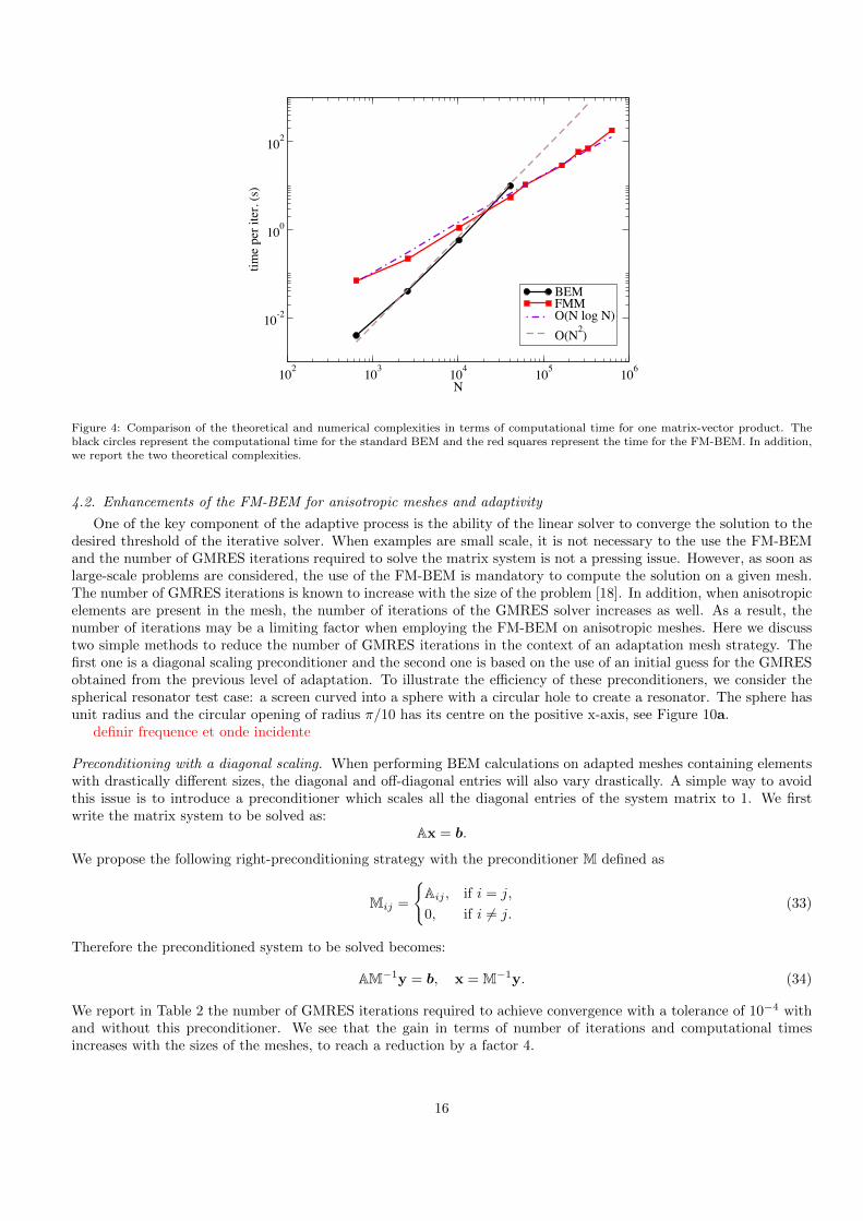
In addition, to check the numerical efficiency of the solver we report in Figure 4 the theoretical and numericalcomplexities in terms of computational time for one matrix-vector product, i.e. the computational time necessary toperform a matrix-vector product with respect to the number of degrees of freedom N . The black circles representthe computational time for the standard BEM and the red squares represent the time for the FM-BEM. As expect,the standard BEM is seen to be of the order of O(N2) operations per iteration and the FM-BEM of the order ofO(N logN) operations per iteration.

15

102 103 104 105 106

N

10-2

100

102

time

per i

ter.

(s)

BEMFMMO(N log N)O(N2)

Figure 4: Comparison of the theoretical and numerical complexities in terms of computational time for one matrix-vector product. Theblack circles represent the computational time for the standard BEM and the red squares represent the time for the FM-BEM. In addition,we report the two theoretical complexities.

4.2. Enhancements of the FM-BEM for anisotropic meshes and adaptivity

One of the key component of the adaptive process is the ability of the linear solver to converge the solution to thedesired threshold of the iterative solver. When examples are small scale, it is not necessary to the use the FM-BEMand the number of GMRES iterations required to solve the matrix system is not a pressing issue. However, as soon aslarge-scale problems are considered, the use of the FM-BEM is mandatory to compute the solution on a given mesh.The number of GMRES iterations is known to increase with the size of the problem [18]. In addition, when anisotropicelements are present in the mesh, the number of iterations of the GMRES solver increases as well. As a result, thenumber of iterations may be a limiting factor when employing the FM-BEM on anisotropic meshes. Here we discusstwo simple methods to reduce the number of GMRES iterations in the context of an adaptation mesh strategy. Thefirst one is a diagonal scaling preconditioner and the second one is based on the use of an initial guess for the GMRESobtained from the previous level of adaptation. To illustrate the efficiency of these preconditioners, we consider thespherical resonator test case: a screen curved into a sphere with a circular hole to create a resonator. The sphere hasunit radius and the circular opening of radius π/10 has its centre on the positive x-axis, see Figure 10a.

definir frequence et onde incidente

Preconditioning with a diagonal scaling. When performing BEM calculations on adapted meshes containing elementswith drastically different sizes, the diagonal and off-diagonal entries will also vary drastically. A simple way to avoidthis issue is to introduce a preconditioner which scales all the diagonal entries of the system matrix to 1. We firstwrite the matrix system to be solved as:

Ax = b.

We propose the following right-preconditioning strategy with the preconditioner M defined as

Mij =

Aij , if i = j,

0, if i 6= j.(33)

Therefore the preconditioned system to be solved becomes:

AM−1y = b, x = M−1y. (34)

We report in Table 2 the number of GMRES iterations required to achieve convergence with a tolerance of 10−4 withand without this preconditioner. We see that the gain in terms of number of iterations and computational timesincreases with the sizes of the meshes, to reach a reduction by a factor 4.

16

# DOFs # iter # iter# DOFs without Prec. with Prec.

152 43 30323 57 37898 77 50

2 051 124 614 031 180 748 163 257 9016 932 412 104

Table 2: Spherical resonator: Number of GMRES iterations required to achieve convergence with a tolerance of 10−4 both without andwith the diagonal scaling preconditioner (33).

Preconditioning strategy based on the use of an appropriate initial guess for GMRES. A further advantage of anadaptive mesh refinement is the possibility to use a computed approximation at a previous level of refinement as aninitial guess for the GMRES solver. This choice is expected to be more efficient than a guess chosen a priori, such asthe zero vector or the incident wave evaluated on the surface. The simple modification consists in interpolating theprevious solution on the new generated mesh (see Step 3 of the refinement strategy, Section 3.6). In our case, this isdone as an additional post-processing step in FEFLO.A. In Table 3, we illustrate the improvement obtained with suchan initial guess. More precisely, we consider the same resonator problem as above and solve the system at each step ofrefinement twice, once with the zero vector as the initial guess and once with the linear interpolation of the previousstep’s numerical solution onto the current mesh as the initial guess. Again the tolerance for the GMRES solver is10−4. The gain is less impressive than the one obtained with the diagonal scaling preconditioner, but an additionalgain of 10% is obtained.

# DOFs # iter # iterwithout Ini. Guess with Ini. Guess

152 30 30323 37 38898 50 45

2 051 61 524 031 74 638 163 90 7716 932 104 90

Table 3: Spherical resonator: number of iterations (with the diagonal scaling preconditioner) with and without the use of an interpolatedinitial guess.

To sum up, the preconditioning by scaling the diagonal entries of the matrix yields to a large reduction of the numberof GMRES iterations. This preconditioning technic shows an increasing gain for meshes having large anisotropic ratios.If the initialization of GMRES by the previous solution helps to save a couple of iterations, this gain increases againwith the size and degree of anisotropy of the mesh.

5. Validation of the adaptive mesh strategy for the FM-BEM

We illustrate in this Section the capabilities of the adaptive mesh strategies for different 3D configurations: scatter-ing of plane waves by open surfaces (planar screen), by closed surface (cavity shape [24]) and finally around a complexgeometry (complex aircraft).

5.1. Planar screen

We consider the scattering of plane waves (with unit amplitude and direction d = (−1, 0, 0)) by a sound-soft unitscreen centered at the origin, i.e., the screen occupies the region

[− 1

2 ,12

]×[− 1

2 ,12

]. Such configurations lead to surface

solutions with the most severe singular behavior, and are a good illustration of the capabilities of an adaptive meshstrategy.

It is well known (see, e.g., [36]) that at the edge of a screen, we have[∂u

∂n

]∼ (kr)−0.5 as kr → 0, (35)

17

where r is the distance from the edge. At the vertices of the screen, this singularity is more severe, and was shown in[8] to take the form [

∂u

∂n

]∼ (kr)−0.704 as kr → 0.

The optimal convergence rate here (for our P1 discretization) is O(N−1). Owing to the singular behavior, the approx-imated solution on a sequence of uniformly refined meshes should yield a sub-optimal convergence rate.

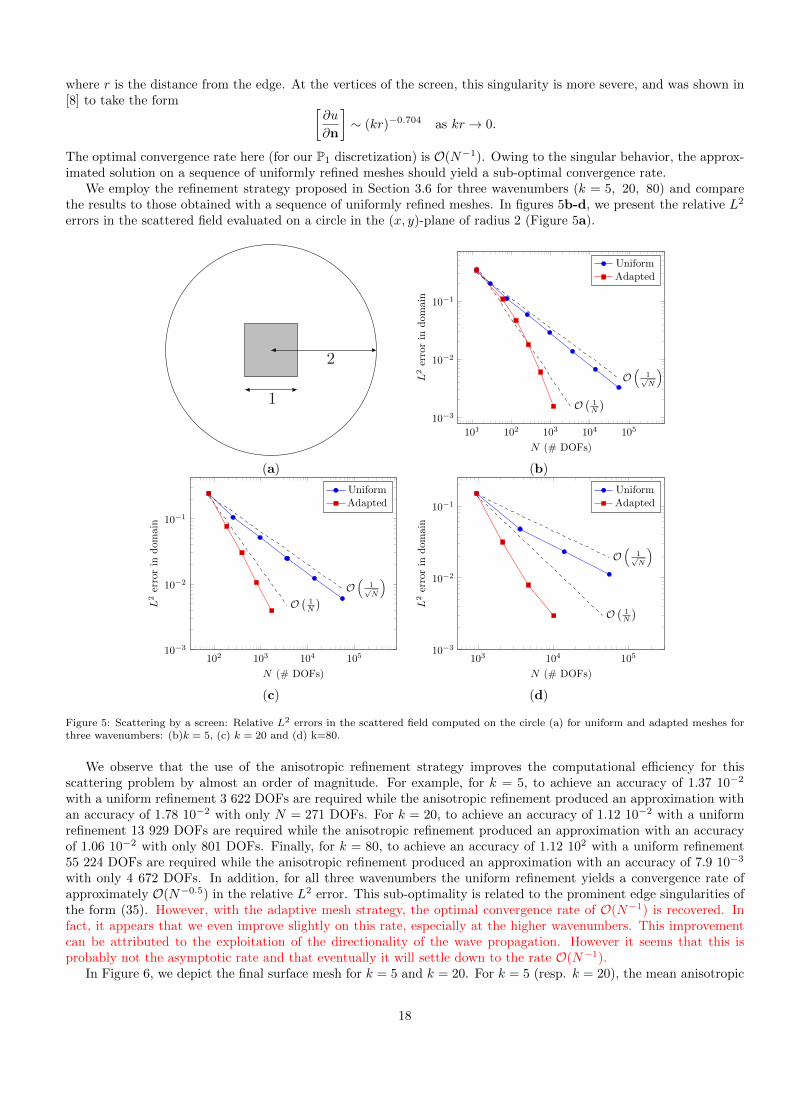
We employ the refinement strategy proposed in Section 3.6 for three wavenumbers (k = 5, 20, 80) and comparethe results to those obtained with a sequence of uniformly refined meshes. In figures 5b-d, we present the relative L2

errors in the scattered field evaluated on a circle in the (x, y)-plane of radius 2 (Figure 5a).

1

2

101 102 103 104 105

10−3

10−2

10−1

O(

1√N

)O(

1N

)

N (# DOFs)

L2

erro

rin

dom

ain

UniformAdapted

(a) (b)

102 103 104 10510−3

10−2

10−1

O(

1√N

)O(

1N

)

N (# DOFs)

L2

erro

rin

dom

ain

UniformAdapted

103 104 10510−3

10−2

10−1

O(

1√N

)

O(

1N

)

N (# DOFs)

L2

erro

rin

dom

ain

UniformAdapted

(c) (d)

Figure 5: Scattering by a screen: Relative L2 errors in the scattered field computed on the circle (a) for uniform and adapted meshes forthree wavenumbers: (b)k = 5, (c) k = 20 and (d) k=80.

We observe that the use of the anisotropic refinement strategy improves the computational efficiency for thisscattering problem by almost an order of magnitude. For example, for k = 5, to achieve an accuracy of 1.37 10−2

with a uniform refinement 3 622 DOFs are required while the anisotropic refinement produced an approximation withan accuracy of 1.78 10−2 with only N = 271 DOFs. For k = 20, to achieve an accuracy of 1.12 10−2 with a uniformrefinement 13 929 DOFs are required while the anisotropic refinement produced an approximation with an accuracyof 1.06 10−2 with only 801 DOFs. Finally, for k = 80, to achieve an accuracy of 1.12 102 with a uniform refinement55 224 DOFs are required while the anisotropic refinement produced an approximation with an accuracy of 7.9 10−3

with only 4 672 DOFs. In addition, for all three wavenumbers the uniform refinement yields a convergence rate ofapproximately O(N−0.5) in the relative L2 error. This sub-optimality is related to the prominent edge singularities ofthe form (35). However, with the adaptive mesh strategy, the optimal convergence rate of O(N−1) is recovered. Infact, it appears that we even improve slightly on this rate, especially at the higher wavenumbers. This improvementcan be attributed to the exploitation of the directionality of the wave propagation. However it seems that this isprobably not the asymptotic rate and that eventually it will settle down to the rate O(N−1).

In Figure 6, we depict the final surface mesh for k = 5 and k = 20. For k = 5 (resp. k = 20), the mean anisotropic

18

ratio is around 30 (resp. 60). If an isotropic error estimate was used, the obtained mesh would contained 55 608DOFs, i.e. 15 times more DOFs than the anisotropic mesh for k = 20 at 5th iteration. This also emphasizes the gainof using anisotropic estimates over isotropic estimates.

Figure 6: Screen case: Final adapted meshes for k = 5 (left) and k = 20 (right).

2nd iteration 3rd iteration 4th iteration 5th iteration

Figure 7: Screen case: Evolution of the anisotropic ratio from 2nd to 5th iteration for k = 20 at side x = 0.5.

Finally, the level of anisotropy on the sides of the screen increases with the complexity, see Figure 7, showing thestrong directionality of the error.

Add complexity, # of iterations and fixed complexity CPU times

5.2. Cube with cavity

We consider the scattering by a cube with cavity [24]. It is a 3D version of the 2D trapping domain [10]. Weuse the refinement strategy for the sound-soft problem and the incident direction is di = (−2,−1,−1) throughout.The singularities in the boundary solution for this problem should be less severe than for the screen. At an edge, the

19

unknown should behave as∂u

∂n∼ r−1/3.

The general rule is that we expect the acoustic pressure u, to behave near an edge as

u ∼ rπ/α as r → 0,

where r is the distance from the edge and α is the exterior angle subtended at the edge. Hence the flow velocity willbehave as

∂u

∂n∼ rπ/α−1 as r → 0.

2102 103 104 105

10−3

10−2

10−1

O(N−

23

)O(N−1

)

N (# DOFs)

L2

erro

rin

dom

ain

UniformAdapted

(a) (b)

103 104 105

10−3

10−2

10−1

O(N−

23

)

O(N−1

)

N (# DOFs)

L2

erro

rin

dom

ain

UniformAdapted

103 104 105

10−3

10−2

10−1

O(N−

23

)O(N−

32

)

N (# DOFs)

L2

erro

rin

dom

ain

UniformAdapted

(c) (d)

Figure 8: Scattering by a sound-soft cube with cavity: Relative L2 errors for uniform and adapted meshes for (b) k = 5, (c) k = 10 andk = 20.

Again, the errors for the adapted and uniform meshes are computed on a circle of radius 2 and are shown inFigure 8b-d for the wavenumbers k = 5, 10, 20. Similarly to the screen problem, the uniform refinement yields asuboptimal convergence rate. However this time the rate is closer to O(N−2/3), i.e., superior to that for the screendue to a less severe singularity.

In Figure 9, we display the mesh at the fourth step of the adaptive process and the real part of the correspondingBEM approximation of the boundary solution. We note, on the top of the cube, the refinement towards the edgesand the exploitation of the directionality. To estimate the gain due to the level of anisotropy, we have generated the

20

equivalent isotropic mesh having the minimal sizes of the anisotropic mesh. The isotropic mesh is composed of 19 409DOFs, i.e. 4 times the number of DOFs in the equivalent anisotropic mesh.

(a) Adapted mesh (b) Real part of the Boundary solution

Figure 9: Cube with cavity: Adapted mesh and real part of the boundary solution at fourth step of the adaptation for the sound-soft cubewith cavity. The incident wave has direction di = (−2,−1,−1) and k = 5.

5.3. Spherical resonator

We consider again the case of a spherical resonator (Figure 10a). Such objects are of interest in the context ofanisotropic mesh refinement because they require the retention of some level of isotropy in the refinement in order tomaintain a good approximation of the surface by planar triangles. The incident wave is a plane wave traveling in thenegative x-direction with a wavenumber of k = 10. In Figure 10b, we represent the modulus of the solution computedin the volume using the boundary integral representation 4.

(a) Uniform mesh with 9 120 vertices (b) Volume solution

Figure 10: Spherical resonator: (a)Uniform mesh of the spherical resonator and (b) corresponding modulus of total field in the (x, y)-plane.

21

Since this example is an isotropic example, we perform an experiment demonstrating the capabilities of our meshrefinement technique with three configurations: with full anisotropy (similarly to what is presented in previous ex-amples), and two additional ones with different levels of isotropy enforced. The first level is called “semi-isotropy”and the second one is a fully isotropic case. For the semi-isotropy approach, the maximum dimension of the adaptedtriangles is limited accordingly to the complexity. Precisely, we enforce

max(h) =C√N,

where h is the maximum dimension of each triangle. This restricts the elongation of the elements but still permitssome elongation controlled by the paramter C. In this work, C is set to 3.5 after some numerical experimentations.

In Figure 11, we give some meshes and corresponding solutions obtained during the adaptation process for thethree strategies.

(a) Mesh and Solution for semi-isotropic adaptation (b) Mesh and Solution for Fully anisotropic adaptation

(c) Mesh and Solution at 3rd level of fully isotropic adaptation (d) Mesh at 6th level of fully isotropic adaptation

Figure 11: Spherical resonator: Adapted meshes with real part of the surface solution for (a) semi-isotropic , (b) fully anisotropic (c) fullyisotropic adaptation strategies, and (d) mesh at 6th level of fully isotropic adaptation. k=5, verifier images et palettes

22

In Figure 12, we report the relative L2 errors for uniform and (anisotropic, isotropic and semi-isotropic) adaptedmeshes with k = 5 verifier que c’est bien le cas car dans les repertoires c’est 11.1. Similarly to the case of the planarscreen, a uniform refinement yields a convergence rate of O(N−

12 ). The anisotropic and semi-isotropic refinement

strategies initially achieve a rate of O(N−32 ) which is super optimal, however this rate begins to slow as higher

accuracies are reached. The reason is that the shape to which the refinement is leading is not the correct one due tothe elongated elements, see Figure 11. By enforcing some isotropy the convergence rate of O(N−

32 ) is maintained up

to a larger mesh. However it still slows once the relative error falls below approximately 10−3. On the other hand, forthe fully isotropic refinement, which restricts the height to width ratio of the triangles, at first the convergence rateis similar to the one obtained by a uniform refinement then for accuracies smaller than 10−2, the convergence rateis O(N−

32 ). Furthermore, it appears that the isotropic refinement maintains this rate asymptotically since it is also

refining towards the spherical shape accurately as well as resolving the edge singularity. Nevertheless, it appears thatif one is interested in achieving accuracies of the order of 10−2 or 10−3, the anisotropic refinement strategy is superior.

102 103 10410−4

10−3

10−2

10−1

O(N−

12

)

O(N−

32

)

N (# DOFs)

L2

erro

rin

dom

ain

UniAniso

Semi-isoIso

Figure 12: Scattering by a spherical resonator: Relative L2 errors for uniform and (anisotropic, isotropic and semi-isotropic) adaptedmeshes with k = 5???.

AJOUTER DES STATS, quels repertoires???This spherical example illustrates the limitations of the current fully anisotropic mesh strategy. In the case of a fully

isotropic solution, the best mesh is obtained with an isotropic mesh strategy in order to preserve the approximationof the geometry. Nevertheless it is possible to use a semi-isotropic strategy to combine the best of the two words: toadapt the mesh by following the directionality of the wave while preserving the curved geometry. Another and morepromising approach consists in defining an adaptive mesh strategy for the P2 interpolation.

5.4. F15 jet

In this test case, we illustrate the robustness of the techniques with respect to the complexity of the input 3Dgeometry. we consider in this case, the geometry of an unarmed F15 jet, see Figure ??. The input plane wave . . .

partie a terminer

6. Conclusion

This paper details the extension of a metric-based anisotropic mesh adaptation strategy within the boundary el-ement method (BEM) for 3D acoustic wave propagation problems. Following the works of [38, 39] for 3D volumesolutions, we have derived the optimal continuous mesh minimizing the P1 interpolation error for 3D surface solu-tions. The method proposed is independent of the discretization technique (e.g., collocation, Galerkin). It completelyremeshes at each refinement step, altering the shape, size and orientations of elements according to the “optimal” met-ric based on a numerically recovered Hessian of the boundary solution. The resulting adaptation is truly anisotropicand we show via a variety of numerical examples that it recovers optimal convergence rates for domains with geometricsingularities: screen, cube with cavity, sphere with cavity or F15 jet.

The first encouraging anisotropic BEM results presented in this work pave the way for further developments. Thefirst important direction is to improve the treatment of curved surfaces. It has been observed numerically that the

23

Figure 13: F15: Left, geometry and right, initial uniform mesh.

level of anisotropy must be controlled to ensure a good approximation of the scatterer’s surface. A more thoroughmethod than the one employed here could be to use two metrics, one based on the recovered Hessian and the otherbased on the surface curvature, and merge them. Another approach is to propose an adaptation strategy for the P2

interpolation. Another necessary improvement concerns the FMM. The version employed in this work is not optimalwith respect to computational times for non uniform meshes. It would be interesting to employ an FMM which istailored to the adapted meshes such as that proposed in [32].

Acknowledgements

This work has been funded by the Agence Nationale de la Recherche (RAFFINE project, ANR-12-MONU-0021).

References

[1] M. Ainsworth and J. T. Oden, A posteriori error estimation in finite element analysis, vol. 37, John Wiley & Sons, 2011.

[2] F. Alauzet and A. Loseille, A decade of progress on anisotropic mesh adaptation for computational fluid dynamics, Computer-Aided Design, 72 (2016), pp. 13–39.

[3] T. Apel, A. Sandig, and J. Whiteman, Graded mesh refinement and error estimates for finite element solutions of elliptic boundaryvalue problems in non-smooth domains, Mathematical methods in the Applied Sciences, 19 (1996), pp. 63–85.

[4] M. Aurada, S. Ferraz-Leite, and D. Praetorius, Estimator reduction and convergence of adaptive bem, Applied NumericalMathematics, 62 (2012), pp. 787–801.

[5] M. Bakry, Fiabilite et optimisation des calculs obtenus par des formulations integrales en propagation d’ondes, PhD thesis, ENSTAParisTech, 2016.

[6] M. Bakry, A goal-oriented a posteriori error estimate for the oscillating single layer integral equation, Applied Mathematics Letters,69 (2017), pp. 133–137.

[7] M. Bakry, S. Pernet, and F. Collino, A new accurate residual-based a posteriori error indicator for the BEM in 2D-acoustics,Computers & Mathematics with Applications, 73 (2017), pp. 2501–2514.

[8] Z. P. Bazant, Three-dimensional harmonic functions near termination or intersection of gradient singularity lines: a generalnumerical method, International Journal of Engineering Science, 12 (1974), pp. 221–243.

[9] M. Bebendorf, Hierarchical matrices, Springer, 2008.

[10] T. Betcke and E. A. Spence, Numerical estimation of coercivity constants for boundary integral operators in acoustic scattering,SIAM Journal on Numerical Analysis, 49 (2011), pp. 1572–1601.

[11] M. Bonnet, Boundary integral equation methods for solids and fluids, John Wiley, 1995.

24

[12] S. Borm, L. Grasedyck, and W. Hackbusch, Introduction to hierarchical matrices with applications, Engineering analysis withboundary elements, 27 (2003), pp. 405–422.

[13] J. Bowman, T. Senior, and P. Uslenghi, Electromagnetic and acoustic scattering by simple shapes, Taylor & Francis Group, 1988.

[14] C. Carstensen, An a posteriori error estimate for a first-kind integral equation, Mathematics of Computation of the AmericanMathematical Society, 66 (1997), pp. 139–155.

[15] C. Carstensen, M. Feischl, M. Page, and D. Praetorius, Axioms of adaptivity, Computers & Mathematics with Applications,67 (2014), pp. 1195–1253.

[16] S. Chaillat and M. Bonnet, Recent advances on the fast multipole accelerated boundary element method for 3D time-harmonicelastodynamics, Wave Motion, 50 (2013), pp. 1090–1104.

[17] S. Chaillat, M. Bonnet, and J. Semblat, A multi-level fast multipole BEM for 3-D elastodynamics in the frequency domain,Computer Methods in Applied Mechanics and Engineering, 197 (2008), pp. 4233–4249.

[18] S. Chaillat, M. Darbas, and F. Le Louer, Fast iterative boundary element methods for high-frequency scattering problems in 3Delastodynamics, Journal of Computational Physics, 341 (2017), pp. 429–446.

[19] S. Chaillat, L. Desiderio, and P. Ciarlet, Theory and implementation of H-matrix based iterative and direct solvers for Helmholtzand elastodynamic oscillatory kernels, Journal of Computational physics, 351 (2017), pp. 165–186.

[20] S. N. Chandler-Wilde, I. G. Graham, S. Langdon, and E. A. Spence, Numerical-asymptotic boundary integral methods inhigh-frequency acoustic scattering, Acta. Numer., (2012), pp. 89–305.

[21] L. Chen, P. Sun, and J. Xu, Optimal anisotropic meshes for minimizing interpolation errors in Lp-norm, Mathematics of Compu-tation, 76 (2007), pp. 179–204.

[22] R. Coifman, V. Rokhlin, and S. Wandzura, The fast multipole method for the wave equation: A pedestrian prescription, IEEEAntennas and Propagation Magazine, 35 (1993), pp. 7–12.

[23] D. Colton and R. Kress, Integral equation methods in scattering theory, SIAM, 2013.

[24] M. Darbas, E. Darrigrand, and Y. Lafranche, Combining analytic preconditioner and fast multipole method for the 3-D Helmholtzequation, Journal of Computational Physics, 236 (2013), pp. 289–316.

[25] E. Darve, The fast multipole method: numerical implementation, Journal of Computational Physics, 160 (2000), pp. 195–240.

[26] B. Faermann, Local a-posteriori error indicators for the Galerkin discretization of boundary integral equations, Numerische Mathe-matik, 79 (1998), pp. 43–76.

[27] M. Feischl, T. Fuhrer, N. Heuer, M. Karkulik, and D. Praetorius, Adaptive Boundary Element Methods: A Posteriori ErrorEstimators, Adaptivity, Convergence, and Implementation, Arch. Computat. Methods Eng., 22 (2015), pp. 309–389.

[28] S. Ferraz-Leite and D. Praetorius, Simple a posteriori error estimators for the h-version of the boundary element method,Computing, 83 (2008), pp. 135–162.

[29] V. Fraysse, L. Giraud, S. Gratton, and J. Langou, Algorithm 842: A set of gmres routines for real and complex arithmetics onhigh performance computers, ACM Transactions on Mathematical Software (TOMS), 31 (2005), pp. 228–238.

[30] T. Gantumur, Adaptive boundary element methods with convergence rates, Numerische Mathematik, 124 (2013), pp. 471–516.

[31] P. George, F. Hecht, and M. Vallet, Creation of internal points in Voronoi’s type method. Control adaptation, Advances inengineering software and workstations, 13 (1991), pp. 303–312.

[32] I. G. Graham, L. Grasedyck, W. Hackbusch, and S. A. Sauter, Optimal panel-clustering in the presence of anisotropic meshrefinement, SIAM Journal on Numerical Analysis, 46 (2008), pp. 517–543.

[33] I. G. Graham, W. Hackbusch, and S. Sauter, Hybrid Galerkin boundary elements on degenerate meshes, Mathematical Aspectsof Boundary Element Methods, 414 (1999), p. 140.

[34] L. Greengard, J. Huang, V. Rokhlin, and S. Wandzura, Accelerating fast multipole methods for the Helmholtz equation at lowfrequencies, IEEE Computational Science and Engineering, 5 (1998), pp. 32–38.

[35] L. Greengard and V. Rokhlin, A fast algorithm for particle simulations, Journal of Computational physics, 73 (1987), pp. 325–348.

[36] P. Juhl, A note on the convergence of the direct collocation boundary element method, Journal of Sound and Vibration, 212 (1998),pp. 703–719.

[37] K. Lipnikov and Y. Vassilevski, Analysis of hessian recovery methods for generating adaptive meshes, in Proceedings of the 15thInternational Meshing Roundtable, Springer, 2006, pp. 163–171.

[38] A. Loseille and F. Alauzet, Continuous mesh framework part I: well-posed continuous interpolation error, SIAM Journal onNumerical Analysis, 49 (2011), pp. 38–60.

[39] , Continuous mesh framework part II: validations and applications, SIAM Journal on Numerical Analysis, 49 (2011), pp. 61–86.

25

[40] M. Maischak, P. Mund, and E. Stephan, Adaptive multilevel BEM for acoustic scattering, Computer methods in applied mechanicsand engineering, 150 (1997), pp. 351–367.

[41] S. Marburg, Discretization requirements: how many elements per wavelength are necessary?, in Computational Acoustics of NoisePropagation in Fluids-Finite and Boundary Element Methods, Springer, 2008, pp. 309–332.

[42] J. Nedelec, Acoustic and electromagnetic equations: integral representations for harmonic problems, vol. 144, Springer Science &Business Media, 2001.

[43] M. Picasso, F. Alauzet, H. Borouchaki, and P.-L. George, A numerical study of some hessian recovery techniques on isotropicand anisotropic meshes, SIAM Journal on Scientific Computing, 33 (2011), pp. 1058–1076.

[44] E. P. Stephan, Boundary integral equations for screen problems in R3, Integral Equations and Operator Theory, 10 (1987), pp. 236–257.

[45] T. Takahashi, A wideband fast multipole accelerated boundary integral equation method for time-harmonic elastodynamics in twodimensions, International Journal for Numerical Methods in Engineering, 91 (2012), pp. 531–551.

[46] M.-G. Vallet, C.-M. Manole, J. Dompierre, S. Dufour, and F. Guibault, Numerical comparison of some hessian recoverytechniques, International Journal for Numerical Methods in Engineering, 72 (2007), pp. 987–1007.

26