metody iloŚciowe w badaniach ekonomicznychqme.sggw.pl/wp-content/uploads/mibe_t13_z2.pdf · metody...

METODY ILOŚCIOWE

W BADANIACH EKONOMICZNYCH

QUANTITATIVE METHODS

IN ECONOMICS

Vol. XIII, No. 2

Warsaw University of Life Sciences – SGGW

Faculty of Applied Informatics and Mathematics

METODY ILOŚCIOWE

W BADANIACH

EKONOMICZNYCH

QUANTITATIVE METHODS

IN ECONOMICS

Volume XIII, No. 2

EDITOR-IN-CHIEF

Bolesław Borkowski

Warsaw 2012

EDITORIAL BOARD

Prof. Zbigniew Binderman – chair, Prof. Bolesław Borkowski, Prof. Leszek Kuchar,

Prof. Wojciech Zieliński, Prof. Stanisław Gędek, Dr. hab. Hanna Dudek, Dr. Agata

Binderman – Secretary

SCIENTIFIC BOARD

Prof. Bolesław Borkowski – chair (Warsaw University of Life Sciences – SGGW),

Prof. Zbigniew Binderman (Warsaw University of Life Sciences – SGGW),

Prof. Paolo Gajo (University of Florence, Italy),

Prof. Evgeny Grebenikov (Computing Centre of Russia Academy of Sciences, Moscow,

Russia),

Prof. Yuriy Kondratenko (Black Sea State University, Ukraine),

Prof. Vassilis Kostoglou (Alexander Technological Educational Institute of Thessaloniki,

Greece),

Prof. Robert Kragler (University of Applied Sciences, Weingarten, Germany),

Prof. Yochanan Shachmurove (The City College of The City University of New York),

Prof. Alexander N. Prokopenya (Brest University, Belarus),

Dr. Monika Krawiec – Secretary (Warsaw University of Life Sciences – SGGW).

PREPARATION OF THE CAMERA – READY COPY

Dr. Jolanta Kotlarska, Dr. Elżbieta Saganowska

TECHNICAL EDITORS

Dr. Jolanta Kotlarska, Dr. Elżbieta Saganowska

LIST OF REVIEWERS

Prof. Iacopo Bernetti (University of Florence, Italy)

Prof. Agata Boratyńska (Warsaw School of Economics)

Prof. Paolo Gajo (University of Florence, Italy)

Prof. Yuiry Kondratenko (Black Sea State University, Ukraine)

Prof. Vassilis Kostoglou (Alexander Technological Educational Institute

of Thessaloniki, Greece),

Prof. Karol Kukuła (University of Agriculture in Krakow)

Prof. Wanda Marcinkowska–Lewandowska (Warsaw School of Economics)

Prof. Yochanan Shachmurove (The City College of the City University of New York)

Prof. Ewa Marta Syczewska (Warsaw School of Economics)

Prof. Dorota Witkowska (Warsaw University of Life Sciences – SGGW)

Prof. Wojciech Zieliński (Warsaw University of Life Sciences – SGGW) Dr. Lucyna Błażejczyk–Majka (Adam Mickiewicz University in Poznan)

Dr. Michaela Chocolata (University of Economics in Bratislava, Slovakia)

ISSN 2082 – 792X

© Copyright by Katedra Ekonometrii i Statystyki SGGW

Warsaw 2012, Volume XIII, No. 2

The original version is the paper version

Published by Warsaw University of Life Sciences Press

CONTENTS

Zbigniew Binderman, Bolesław Borkowski, Wiesław Szczesny – Radar coefficient of concentration .............................................................. 7

Mariola Chrzanowska – Differences in results of ranking depending on the frequency of the data used in multidemensional comparatine analysis. Example of the stock exchanges in Central-Eastern Europe ....... 22

Stanisław Jaworski – Comparison of the beef prices in selected countries of the European Union ................................................................................. 31

Stanisław Jaworski, Konrad Furmańczyk – Unemployment rate for various countries since 2005 to 2012: comparison of its level and pace using functional principal component analysis .................................. 40

Krzysztof Kompa – Comparison of capital markets in Bulgaria, Romania and Slovakia in years 2001-2009 ................................................. 48

Krzysztof Kompa – Index of Central and East European securities quoted at Warsaw Stock Exchange - WIG-CEE ..................................................... 60

Lucyna Kornecki, E. M. Ekanayake – A research note: State based factors affecting inward FDI employment in the U.S. economy ................. 73

Monika Krawiec – Testing the Granger causality for commodity mutual funds in Poland and commodity prices ....................................................... 84

Piotr Łukasiewicz, Krzysztof Karpio, Arkadiusz Orłowski – Changes of distributions of personal incomes in US from 1998 to 2011 ................... 96

Magdalena E. Sokalska – Comparison of intraday volatility forecasting models for polish equities ........................................................................... 107

Dorota Witkowska – Wage disparities in Poland: Econometric analysis ........... 115

Olga Zajkowska – Is there a representative polish unemployed female?- Microeconometric analysis .......................................................................... 125

Wojciech Zieliński – An application of the shortest confidence intervals for fraction in controls provided by Supreme Chamber of Control ............. 134

QUANTITATIVE METHODS IN ECONOMICS Vol. XIII, No 2, 2012, pp. 7 – 21

RADAR COEFFICIENT OF CONCENTRATION

Zbigniew Binderman Department of Econometrics and Statistics,

Warsaw University of Live Sciences - SGGW e-mail: [email protected]

Bolesław Borkowski Department of Econometrics and Statistics,

Warsaw University of Live Sciences – SGGW Warsaw University, Faculty of Management

e-mail: [email protected] Wiesław Szczesny

Department of Informatics, Warsaw University of Live Sciences – SGGW e-mail: [email protected]

Abstract: In the following work we have described a process of using radar charts to measure concentration of a distribution. The process utilises the idea of Gini index based on a Lorenz curve as well as a method presented by the authors in [Binderman, Borkowski, Szczesny 2010]. The presented technique can also be used by analysts to create new coefficients of concentration based on measures of similarity and dissimilarity of objects so that from the set of constructed coefficients one that best fulfils the required criteria of sensitivity can be chosen.

Keywords: Gini index, Schutz’s measure, radar coefficient of concentration, radar method, radar measure of conformability, measure of similarity, synthetic measures, classification, cluster analysis

INTRODUCTION

One of task that are given to analysts is to present concentration (non-uniformity in terms of possession) of a “resource” and the level of its changes in a given time frame in a clear and simple manner. For example it can be the change of concentration of accrued gains for clients of a commercial bank, non-uniformity of salary in a corporation, the level of concentration of land ownership by private

8 Zbigniew Binderman, Bolesław Borkowski, Wiesław Szczesny

household in Poland or, by expanding the definition of non-uniformity, presentation of a demographical structure valuation on a given geographical area. Analysts often do not possess data on a level of a single object. On the other hand, they do have access to data in tabular form. Which means performing analysis based on aggregated data, essentially using data in a form of a set of vectors, which coordinates describe directly or indirectly the structures in question. Bibliography in the field of measurement of similarity or dissimilarity of structures provides a rich set of instruments. The most important Polish publications are [Chomątowski, Sokołowski 1978, Kukuła 1989, 2010, Strahl 1985, 1996, Strahl (red.) 1998, Walesiak 1983, 1984 et al]. However, only few of them could have been inspired by visualization, i.e. graphical representation of structures (see. Binderman, Borkowski, Szczesny 2009, 2010a, 2010b, 2010c; Borkowski Szczesny 2002, 2005; Binderman, Szczesny 2009, 2011; Binderman 2011; Ciok 2004; Ciok, Kowalczyk, Pleszczyńska, Szczesny 1995]). Moreover, not every visualization technique is easily applicable when representing a larger number

of structures. Additionally, it is worth mentioning, that the consumer of the analysis is most often expecting conclusions supported by values of appropriate measures having straightforward interpretation but also intuitive charts. However, present day, basic office tools allow to relatively easily implement simple methods of measuring structures' similarity as well as visualization thereof. Only very complex techniques require support from specialized equipment to perform measurement and visualization.

Authors have been engaged in the research on measuring similarity or dissimilarity of structure, especially in the field of economical-agricultural studies, in both static and dynamic approaches (see [Binderman, Borkowski, Szczesny, Shachmurove 2012, Binderman, Borkowski, Szczesny 2008, 2009, 2010b,c; Borkowski Szczesny 2002]). Bibliography in this fields provides a rich set of instruments.

The word “structure” can have multiple meanings depending on context, i.e. an economical structure, agricultural structure and so on. An in-depth analysis of the term structure in relation to economical studies was performed in [Kukuła 2010, Malina 2004].

Let

1 2

1 21

1 20

1

, ,...,: ( , ,..., ) : , , ,

: ( , ,..., ) : .

nn i

nn

n ii

nx x x x i n

x x x x

+

+=

ℜ = = ≥ = ∈

⎧ ⎫Ω = = ∈ℜ =⎨ ⎬⎩ ⎭

∑

x

x

In the following work the elements of set Ω will be called structural vectors or structures for short.

Radar coefficient of concentration 9

Let X denote any non-empty set, function : X X : ( , )× →ℜ = −∞ +∞d for any two elements x, y from X fulfills the following:

1. (x, y) 0,≥d 2. (x, x) 0,=d 3. (x, y) (y, x)=d d .

Function d(x, y) can be treated as a measure of dissimilarity of elements x and y. In literature it is often called distance. However, it needs to emphasized that this is not a metric. Naturally, every metric is a distance. A diameter of set X will be equal to: .

X

X,: sup ( , )

x yx y

∈ρ = d

. We will say a function : X X [0,1]× →s is a measure of similarity when for any two elements x and y from set X it fulfills:

1. s(x,x)=1, 2. s(x,y)=s(y,x).

Let the diameter of set X - X 0ρ > be finite. Let us notice that using the measure of dissimilarity of elements d we can define the measure of similarity by equation:

X

x,yx,y 1 ( )( ) = −ρd

ds

. In a special case when X 1ρ = the above equation takes form:

x,y 1 x,y( ) ( )= −ds d . With the development of techniques of visualization analysts started to utilize heuristic measures, which are intuitive and seem to be a promising path of advance, in order to compare ordering of objects. Visualization of objects, which have many features, based on polygons (i.e. radar charts from MS EXCEL) is one of such techniques. Authors have dedicated a few works to this problem [see Binderman, Borkowski, Szczesny 2008, 2010a, 2011]. Let us define a synthetic pseudo-radar measure of vector 1 2( , ,..., )nx x x=x ∈ n]1;0[ as [por. Binderman, Borkowski, Szczesny 2008]:

( ) 1 1 1

1

1R , :n

i i ni

x x x xn + +

=

= =∑x.

(1)


This measure is normalized (i.e. it takes values from interval [0, 1]) and allows to define in various ways the function of dissimilarity (distance) of two given objects

1 2( , ,..., ),nx x x=x 1 2( , ,..., )ny y y= ∈Ωy . For example:

1 2( , ) ( ) ( ) , ( , ) ( )d R R d R= − = −x y x y x y x y , (2)

where ( )1 1 2 2: , ,..., n nx y x y x y− = − − −x y .

The above “distances” induce measures of similarity of structures:

1 2 1 2( , ,..., ), ( , ,..., )n nx x x y y y= = ∈Ωx y :

1 21 2, 1 , , 1 ,( ) ( ), ( ) ( )= − = −x y x y x y x yd ds d s d . (2’)

Example 1. Let 1 1 1 10 02 2 2 2, , , , ,⎛ ⎞ ⎛ ⎞= =⎜ ⎟ ⎜ ⎟

⎝ ⎠ ⎝ ⎠x y , then

1 102 2, ,⎛ ⎞− = ⎜ ⎟

⎝ ⎠x y

( ) ( ) 1R R2 3

( )R= = − =x y x y , 1 210

2 3( , ) , ( , )d d= =x y x y , which

implies 1

, 1( ) ,=x yds 2

1, 12 3

( ) = −x yds ,

where measures d1, d2, s1, s2 are defined as in (2), (2’), respectively.

MEASUREMENT OF CONCENTRATION

Economic inequality was for a long time in the center of attention of both, sociologists and economists. However, the meaning of that term is not precisely defined. Naturally, it is easy to differentiate between a state of equality and inequality, but given two non-uniform distributions of a resource it is non-trivial to determine which of the two is “more” unequal. In general it is accepted that a distribution where each household possesses the same income is called an egalitarian distribution, one that is void of any inequality. When studying inequality one measures the degree to which the studied distribution differs from an egalitarian one. To measure the degree of dissimilarity (concentration) one must decide on a particular measure. However, a choice of a measure in practice means a decision on how to specifically define inequality/concentration.

As mentioned in the introduction we will limit ourselves to aggregated data, which means henceforth x, y∈Ω denote two structures, where y denotes a structure of objects divided into quintile groups, meaning having uniform coordinates equal to 1/n, while x denotes a structure of a resource associated with those n groups of objects contained in structure y. This does not decrease the level of generality of our analysis as a population of size n can be defined by two structures with n coordinates.


We will call the following a cumulation of a vector 1 2 nx x x=x ( , ,..., )∈Ω

cum(x):= ( )1 1 1

^ ^ ^ ^1 2

1 1 1, ,..., ,1 , ,...,i i i n

i i ix x x x x x

= = =

⎛ ⎞ = =⎜ ⎟⎝ ⎠∑ ∑ ∑ x .

Practicians who study levels of differentiation of income or other resources possessed by a given group of objects most often present the following postulates about coefficient d(x, y) used for measurement (which deals in a case of aggregated data with dissimilarity between structures of entities and resources possessed by those entities): • coefficient assumes the value of 0 if the resource is uniformly distributed across

all objects (the structures are identical x = y); • values of the coefficient are consistent with principle of transfers, which states

that any transfer of resources between a “poorer” object to a “richer” one increases the non-uniformity in the population (which means that transfers between components of the structure, xi and xi+s increases the values of d(x, y));

• transfer sensitivity axiom : the influence a transfer from a “poor” object to a “poorer” one has on the value of the coefficient, when the value of the transfer is constant, is greater the richer the giving object is (which means that the farther away the giving object is from the receiving one, the greater the change of the value of dissimilarity should be);

• coefficient d(x, y) assumes its maximum when all the resources are possessed by a single object (in case of dissimilarity of two structures when, for example, x = (0, 0, …, 0, 1));

• scale invariance axiom means that the value of the coefficient does not change when the values of resources experience proportionate changes.

Naturally, the fourth postulate can be omitted because it follows from the second postulate.

The most popular coefficient used to measure the level of concentration (dissimilarity) of distribution, which fulfills the above postulates, is the Gini index, defined as doubled area between the Lorenz curve and the diagonal of a unit square (see [Barnett 2005, Hoffmann and Bradley 2007]).

In order to present the construction of a basic coefficient of dissimilarity (concentration) of distribution based on radar charts, let us inscribe a regular n-gon Fn into a unit circle with a radius of 1 and centered at the origin of in the Cartesian coordinate system in the Euclidean plane (z,w)=(0,0). Let us connect the vertices of the n-gon with the origin of the coordinate system. We will denote the resulting line segments of length 1 as O1, O2, …, On, starting with the segment covering the vertical axis w. If the features of object x=(x1,x2,...,xn) assume unit values from the interval <0, 1>, that is 0≤x≤1 ≡ 0 ≤ xi ≤1, i=1,2,...n,, where 0 = (0, …, 0) and 1 = (1, …, 1), then we can present the values of features of this object on a radar chart. To do this, let us


denote by xi a point on Oi, which was constructed by intersecting the segment Oi with a circle of radius xi and centered at the origin of the coordinate system, for i = 1, 2, …, n. By connecting x1 with x2, x2 with x3, …, xn-1 with xn and xn with x1 we will construct a polygon Wn.

In the following figure 1 (radar chart) we find illustrations for vectors representing structures:

y =

1 1 1 14 4 4 4, , , ,⎛ ⎞= ⎜ ⎟

⎝ ⎠1 / 4 ⎟

⎠⎞

⎜⎝⎛=

169,

164,

162,

161x (3)

and their respective vectors representing those structures when they are in cumulative form: cum(1/4)=(1/4,2/4,3/4,1) i cum(x)=(1/16,3/16,7/16,1).

Figure 1. Left: illustration of structures defined as in (3). Right: illustration of structures as defined in (2) in cumulative form.

00,1

0,20,3

0,4

0,5

0,6O1

O2

O3

O4

1/4x

0

0,2

0,4

0,6

0,8

1O1

O2

O3

O4

cum(1/4)

cum(x)

Source: own research

Let us notice that polygon representing cum(x) is contained within a polygon induced by vector cum(1/4). Let vector 1 2

' ' '' ( , ,..., )nx x x=x denote any structure

( '∈Ωx ) which coordinates fulfill the condition 1 2 nx x x≤ ≤ ≤' ' ': ... . It can be proved that a polygon designated by cum(x') is contained within a polygon designated by cum(1/n) for n >= 4.

THEOREM 1.

Let a vector 1 2 nx x x=x ( , ,..., )∈Ω, n∈ , the structure 1 2' ' '' ( , ,..., )nx x x=x

means the vector, created by the permutation of the coordinates of the vector x, that its coordinates satisfy the condition 1 2 nx x x≤ ≤ ≤' ' ': ... . We denote by


( )^ ^ ^ ^1 2, ,..., nx x x=x the cumulation of the vector x ' i.e. x^=cum( x '). If the radar

polygons ^ ^,x 1

n

W W are generated by vectors ^

^ i 1xn

, respectively, then

^ ^⊂x 1

n

W W .

Proof. Let us suppose that the assumption of the theorem are satisfied but ^ ^ ^ ^and⊃ ≠

x x1 1n n

W W W W . This means that there exists k∈1,2, ..., n-1 such

that ^k

kxn

> . The last inequality and the definition of the vector x ' together imply

' ' '

11, 2, ...,

1 1, and x fork

i k ji

j k k nkx xn n n=

= + +> > >∑.

Hence ^ , 1, ...,x forj j k k nkn

= +> . In particular, ^x 1nnn

> = , which contradicts

the assumption. Thus ^ ^⊂x 1

n

W W for all x∈Ω. The last inequality follows from

the turn that ^ , 1, ...,x dlaj j k k nkn

= +> . In particular, that ^x 1nnn

> = . But with

the notion we have that ^x 1n = , this contradicts our assumption, therefore, that

^ ^ ^ ^i⊃ ≠x x1 1

n n

W W W W .

Which is similar to the situation when a polygon designated by the abscissa

and the Lorenz curve is contained within any triangle of a unit square. More precisely, a polygon designated by the abscissa and a cumulated structure of a resource is contained within a polygon designated by the abscissa and a cumulated specialization of structure of a resource, which is identical with the structure of objects – meaning when the resource is uniformly distributed across all objects.

For the considered example of vectors x and y in the following figure 2, we have presented a structure of a resource defined by vector x compared against an egalitarian structure (one with uniform coordinates) in both forms, normal and cumulated (both as column charts – left part of figure 2) as well as in the form of a Lorenz curve (right part of figure 2). It can be easily seen that in this case the Lorenz curve is identical to with the so called curve of cumulated frequency of a resource placed on four intervals of equal length into which the interval [0, 1] was divided. Let us notice that the classic Gini index in this example is equal to the complement to 1 for the ratio of two areas: one underneath the Lorenz curve and


other beneath cum(1/4). We will denote this coefficient as G. Using the remaining two geometrical interpretations (radar polygon and column chart for cumulated structure) in a similar manner, we arrive at two coefficients GR and GS that measure the non-uniformity of the distribution. It can be easily show that in the case of structure (1/16, 2/16, 4/16, 9/16) we have G=0,40625, GR=0,6041(6), GS=0,3250.

Figure 2. Presentation of structures (2) in normal and cumulated form

0

0,1

0,2

0,3

0,4

0,5

0,6

0,7

0,8

0,9

1

0 0,2 0,4 0,6 0,8 1

cum(x)=Lorenc C

cum(1/4)

00,1

0,20,30,4

0,50,6

x1 x2 x3 x4

1/4x

0

0,2

0,4

0,6

0,8

1

x1 x2 x3 x4

cum(1/4) cum(x)


However, it needs to be mentioned that both coefficients G and GS, when there is a low amount of objects (in this case a low amount of coordinates of vector x), meaning when all of the resource in in the possession of a single object, assume values far removed from 0. Specifically, for x = (0, 0, 0, 1) we have symbol G=0,75, GS=0,60 i GR=1,0. After introducing normalizing factors (meaning after dividing by 0,75 and 0,6, respectively), for the previously considered structure (1/16, 2/16, 4/16, 9/19) we receive values G=0,40625/0,75 = 0,541(6) = GS=0,3250/0,60. In general, the area S1 of a radar polygon induced by vector x=(x1,x2,...,xn) ∈[0,1]n is defined as follows [Binderman, Borkowski, Szczesny 2008]:

n n

1 i i 1 i i 1 n 1 1i 1 i 1

1 2 22 n n

1x x sin sin x x , gdzie x : x .2S + + += =

π π== =∑ ∑

Which means is can be shown that area S0 of a radar polygon Fn, induced by vector cum(1/n) = (1/n, 1/n, …, 1/n) is defined by:


1 1 1

0 21 1 1 1

2

1 2 1 1 2 ( 1) 1sin sin2 2

2 4 2sin12

n i i n

j ji j j i

i iS x xn n n n n

nn n

π π

π

− + −

= = = =

⎛ ⎞⎛ ⎞⎛ ⎞ +⎛ ⎞= + = + =⎜ ⎟⎜ ⎟⎜ ⎟ ⎜ ⎟⎜ ⎟ ⎝ ⎠⎝ ⎠⎝ ⎠⎝ ⎠+=

∑ ∑ ∑ ∑

It can be easily proved that if 1 2 nx x x= ∈Ωx ' ' '' ( , ,..., ) has this

1 2' ' ': ... nx x x≤ ≤ ≤ property, that its coordinates fulfill then radar polygon Wn

induced by vector cum(x') is contained in radar polygon Fn, induced by vector cum(1/n). The ratio of areas of those polygons S1/S0 can be assumed to be the measurement of similarity of a given structure (distribution of a resource) to a uniform structure (egalitarian distribution) and a coefficient defined as:

1^ ^ ^ '1

1 121 10

61 1 , gdzie :2 4

n i

i i i ji j

S nR x x x x xS n

−

+= =

⎡ ⎤= − = − + =⎢ ⎥+ ⎣ ⎦∑ ∑G (4)

can be assumed to be a measurement of concentration/non-uniformity of distribution of a resource set by structure x'. It is easy to show, that measure GR(1/n)=0, GR((0,…,0,1))=1.

DEFINITION

A measurement defined by equation (4) will be called a radar measure of concentration (non-uniformity of income).

The radar measure fulfills the 5 previously mentioned postulates set by practicing. Let us notice that Gini index, fulfilling the postulates, has this property that G(1/n)=0 i G((0,…,0,1))=1-1/n. However, if we desire for it to assume a value of one for the structure (0, 0, …, 1), we can multiply it by n/(n – 1). Using the same idea of a geometrical interpretation we can transform (symbol) the equation for the measure when we are using a column chart to:

^

1 ^

1

1

min[ ), ]21 =1- min( , ) ,

1

n

i i ni

i ini

ii

x yS x y

ny

=

=

=

⎡ ⎤⎢ ⎥⎣ ⎦= −

+⎡ ⎤⎢ ⎥⎣ ⎦

∑∑

∑G (5)

^ 'i

1gdzie x , , 1,...,

i

i jj

ix y i nn=

= = =∑.

Naturally, coefficient GS also fulfills the conditions postulated by practicians, but for the structure (0, 0, …, 1) is assumes a value of (n – 1)/(n + 1). However, after normalization (meaning multiplying by a factor of (n + 1)/(n – 1)) it is equal to the value of a normalized Gini index. This is why we will not be considering this coefficient any more.


Another means of creating a measure of concentration is by using measures of dissimilarity of structures in cumulated form and the same idea that was behind the Gini index (where “distance” is the area between a Lorenz curve and the diagonal). Meaning, by using the technique of radar coefficients it can be shown that a coefficient defined as:

1 2

1 2

[( , ,...,1), ( )], 1, 2,

[( , ,...,1), (0,0,...,0,1)]k n n

kk n n

dW kd

= =cum x

(6)

where dk is defined by equation (2). Those coefficients also fulfill the previously mentioned postulates. Overall, an analyst can create many such coefficients.

COEFFICIENTS' SENSITIVITY TO CHANGES

Whenever we are faced with a problem of comparing non-uniformity of distribution of a resource between objects in multiple populations or in one population but in multiple time periods, there is a risk that it can't be done by visualization alone. We need to possess a non-uniformity coefficient which is sensitive to that special type of changes of non-uniformity that interest the researcher/analyst. Because the most popular Gini index may prove to be unresponsive to the aspect of changes that the analyst wants to study. Naturally, the study of sensitivity of various coefficients requires an appropriate mathematical workshop. However, today, with the ubiquitous computer tools, it can be achieved by utilizing simple office tools. Let us show this on an artificial example. Let us assume we are interested in the disappearance of the so called middle class and we want to test whether the coefficient GR is more sensitive to that change than Gini index. In table 1 we can see changes of fictitious structure of, for example, salaries in a big corporation in various time periods or, perhaps, the changes of the structure of income from all possible sources in a given society. For simplification purposes, let us assume our data is aggregated to decile (nie jestem pewien czy to jest dobre tłumaczenie) groups. In Table 2 we present the values of six coefficients of concentration. The first three are the well-known coefficients based on the Lorenz curve: Gini, Schutz and L=(l- 2 )/(2- 2 ), where l the length of the Lorenz curve (see Barnett R. 2005, Hoffmann and Bradley 2007, Kakwani 1980, Lamber 2001, Rosenbluth 1951). The latter three are based on visualization methods that use radar charts. Coefficients Gr1 and Gr2 were created by applying formula (6) to equation (2).

The data was compiled in such a manner that we begin with a structure that possesses a large middle class, composing 50% of the whole population and owning 80% of the resources. Afterwards, we add the rich class. During the studied period there is a large outflow of resources from the middle class to the rich class and a small outflow from the middle class to the poor one. We are interested in such a coefficient that would signalize those changes by increasing its value.


Table 1. Fictitious structures: egalitarian (T0), and during seven periods (T1, …, T7) d1 d2 d3 d4 d5 d6 d7 d8 d9 d10

T0 0,1 0,1 0,1 0,1 0,1 0,1 0,1 0,1 0,1 0,1T1 0,00000 0,01000 0,02000 0,02000 0,05000 0,18000 0,18000 0,18000 0,18000 0,18000T2 0,00889 0,01000 0,02000 0,02000 0,05000 0,16000 0,18000 0,18000 0,18000 0,19111T3 0,00889 0,02000 0,04000 0,05000 0,05000 0,06000 0,18000 0,18000 0,18000 0,23111T4 0,00889 0,02625 0,06000 0,06000 0,06000 0,06000 0,08000 0,18000 0,18000 0,28486T5 0,00889 0,02750 0,07000 0,07000 0,07000 0,07000 0,07000 0,08000 0,18000 0,35361T6 0,00989 0,04262 0,07000 0,07000 0,07000 0,07000 0,07000 0,07000 0,07000 0,45749T7 0,05311 0,05311 0,05311 0,05311 0,05311 0,05311 0,05311 0,05311 0,05311 0,52200 Source: own research

Table 2. Coefficients of concentration during the studied periods

Gini Schutz L GR Gr1 Gr2

T1 0,4220 0,4000 0,2247 0,4698 0,2718 0,4834T2 0,4220 0,3911 0,2126 0,4799 0,2788 0,4820T3 0,4220 0,3711 0,1803 0,5194 0,3067 0,4714T4 0,4220 0,3449 0,1670 0,5572 0,3346 0,4626T5 0,4220 0,3336 0,1736 0,5872 0,3575 0,4549T6 0,4220 0,3575 0,2010 0,6216 0,3849 0,4538T7 0,4220 0,4220 0,2327 0,6277 0,3898 0,4528

Lorenz Curve Radar's diagram


Table 2 shows that the most popular Gini index is not sensitive to those changes in the structure, that are defined in Table 1, while radar coefficients GR and Gr1 clearly show that changes towards increasing the level of concentration are happening. On the other hand, coefficient Gr2 indicates that the level of concentration is decreasing. Schutz and L coefficients are behaving in a similar fashion, but only during periods T1 – T5. We leave the decision which of those coefficients is best at picking up changes in times of increasing globalization. Naturally, such a decision requires defining which features are preferable.

In order to present in a more intuitive manner the idea of sensitivity of those coefficients to changes, we will consider the initial structure of resources s0 defined in Table 3 and we will assume that further changes to it will involve transferring 0.01 of a resource from group d1 to groups d2, d3, …, d10. We will denote structure created by these transfers as s1, …, s9. The values of the six chosen coefficients are present in Table 4, while the values of deltas of them are in Table 5 and Figure 3.


Table 3. Exemplary initial structure of resources for the purposes of the simulation d1 d2 d3 d4 d5 d6 d7 d8 d9 d10

s0 0,019 0,021 0,04 0,06 0,08 0,1 0,12 0,14 0,16 0,26 Source: own research

Table 4. Values of the chosen coefficients of concentration for the structure defined in Table 3 and its nine subsequent modifications involving transfers of resources from group d1 to other decile groups

s0 s1 s2 s3 s4 s5 s6 s7 s8 s9

Gini 0,3842 0,3862 0,3882 0,3902 0,3922 0,3942 0,3962 0,3982 0,4002 0,4022Schutz 0,2800 0,2800 0,2800 0,2800 0,2800 0,2900 0,2900 0,2900 0,2900 0,2900L 0,1350 0,1369 0,1396 0,1419 0,1437 0,1450 0,1459 0,1467 0,1472 0,1486GR 0,4998 0,5029 0,5032 0,5037 0,5045 0,5058 0,5077 0,5104 0,5138 0,5184Gr1 0,2928 0,2949 0,2951 0,2955 0,2961 0,2970 0,2984 0,3003 0,3027 0,3060Gr2 0,4192 0,4200 0,4215 0,4237 0,4262 0,4288 0,4315 0,4340 0,4360 0,4371 Source: own research

Figure 3. Increases of values of coefficients from Table 3. detailed information can be found in Table 5.

0,0000

0,0005

0,0010

0,0015

0,0020

0,0025

0,0030

0,0035

0,0040

0,0045

0,0050

s1 s2 s3 s4 s5 s6 s7 s8 s9

Gini L GR

Gr1 Gr2


It is clear in the figure that the increase of Gini index is constant and equal to 0,002. However, individual increases of other coefficients have differed substantially. Radar coefficient GR reacts more strongly than Gini index to transfers from d1 to d2 or d10, while experiencing lower changes when transfers


happen from d1 to d2 – d6. Which means that is displays a “sharper” reaction to creation of rich and poor groups.

Table 5. Changes (increases) in values of coefficients of concentration from Table 3. s0 s1 s2 s3 s4 s5 s6 s7 s8 s9

Gini x 0,0020 0,0020 0,0020 0,0020 0,0020 0,0020 0,0020 0,0020 0,0020Schutz x 0,0000 0,0000 0,0000 0,0000 0,0100 0,0000 0,0000 0,0000 0,0000L x 0,0019 0,0027 0,0023 0,0018 0,0013 0,0010 0,0007 0,0005 0,0014GR x 0,0031 0,0003 0,0005 0,0009 0,0013 0,0019 0,0026 0,0034 0,0046Gr1 x 0,0022 0,0002 0,0004 0,0006 0,0009 0,0014 0,0019 0,0025 0,0033Gr2 x 0,0008 0,0015 0,0021 0,0025 0,0027 0,0027 0,0025 0,0021 0,0011 Source: own research

SUMMARY

In this work we have presented two approaches to creating coefficients of concentration as well as basic technique for verification of fitness for purpose of the created coefficients, which can be easily performed with standard office applications. Naturally, a more elegant approach is to deduce the properties of constructed coefficients by means of instruments provided by higher level mathematics. However, performing numerous well-planned simulations can not only simplify that process but also replace it altogether. Results that we have got for fictitious data show the strong suits of methods that use radar charts. Authors intend to verify their presented conceptions in their next work by using real data.

REFERENCES

Barnett R. A. et al. (2005) College Mathematics for Business, Economics, Life Sciences, and Social Sciences, 10th ed., Prentice-Hall, Upper Saddle River.

Binderman, Z., Borkowski B., Szczesny W., Shachmurove Y. (2012): Zmiany struktury eksportu produktów rolnych w wybranych krajach UE w okresie 1980-2010, Quantitative Methods in Economics Vol. XIII, nr 1, 36-48.

Binderman, Zb., Borkowski B., Szczesny W. (2011) An Application Of Radar Charts To Geometrical Measures Of Structures’ Of Conformability, Quantitative methods in economics Vol. XII, nr 1, 1-13.

Binderman Z., Borkowski B., Szczesny W. (2010a) Radar measures of structures’ conformability, Quantitative methods in economy XI, nr 1, 1-14.

Binderman Z., Borkowski B., Szczesny W. (2010b) Analiza zmian struktury spożycia w Polsce w porównaniu z krajami unii europejskiej. Metody wizualizacji danych w analizie zmian poziomu i profilu konsumpcji w krajach UE, , RNR PAN, Seria G, Ekonomika Rolnictwa , T. 97, z. 2, s. 77-90.

Binderman Z., Borkowski B., Szczesny W. (2010c) The tendencies in regional differentiation changes of agricultural production structure in Poland, Quantitative methods in regional and sectored analysis, U.S., Szczecin, s. 67-103.


Binderman Z., Borkowski B., Szczesny W. (2009) Tendencies in changes of regional differentiation of farms structure and area Quantitative methods in regional and sectored analysis/sc., U.S., Szczecin, s. 33-50.

Binderman Z., Borkowski B., Szczesny W. (2008) O pewnej metodzie porządkowania obiektów na przykładzie regionalnego zróżnicowania rolnictwa, Metody ilościowe w badaniach ekonomicznych, IX, 39-48, wyd. SGGW.

Binderman Z., Szczesny W. (2009) Arrange methods of tradesmen of software with a help of graphic representations Computer algebra systems in teaching and research, Siedlce Wyd. WSFiZ, 117-131.

Binderman Z., Szczesny W. (2011) Comparative Analysis of Computer Techniques for Visualization Multidimensional Data, Computer algebra systems in teaching and research, Siedlce, wyd. Collegium Mazovia, 243-254.

Borkowski B., Szczesny W. (2005) Metody wizualizacji danych wielowymiarowych jako narzędzie syntezy informacji, SERiA, Roczniki Naukowe, t. VII, 11-16.

Binderman Zb. (2011): Matematyczne aspekty metod radarowych, Metody Ilościowe w Badaniach Ekonomicznych, XII, nr 2, 69-79.

Chomątowski S., Sokołowski A. (1978) Taksonomia struktur, Przegląd Statystyczny, nr 2, s. 14-21

Ciok A. (2004) Metody gradacyjne analizy danych w identyfikacji struktur wydatków gospodarstw domowych. Wiadomości Statystyczne Nr 4, s. 12 - 21

Ciok A., Kowalczyk T., Pleszczyńska E., Szczesny W. (1995) Algorithms of grade correspondence-cluster analysis. The Coll. Papers on Theoretical and Aplied Computer Science, 7, 5-22.

Hoffmann . L. D. and Bradley G. L. (2007) Calculus for Business, Economics, and the Social and Life Sciences, 9th ed., McGraw Hill, New York.

Kakwani N. C. (1980) Income inequality and poverty, methods of estimations and policy applications, Oxford University Press, New York.

Kukuła K. (1989) Statystyczna analiza strukturalna i jej zastosowanie w sferze usług produkcyjnych dla rolnictwa, Zeszyty Naukowe, Seria specjalna Monografie nr 89, AE w Krakowie, Kraków.

Kukuła K. (red.) (2010) Statystyczne studium struktury agrarnej w Polsce, PWN, Warszawa.

Lamber P.,J. (2001) The distribution and redistribution of income, Manchester University Press.

Malina A. (2004) Wielowymiarowa analiza przestrzennego zróżnicowania struktury gospodarski Polski według województw. AE, S. M. nr 162, Kraków.

Rosenbluth G. (1951) Note on Mr. Schutz’s Measure of income inequality, The American Economic Review, Vol. 41, no. 5, 935-937.

Szczesny W. (2002) Grade correspondence analysis applied to contingency tables and questionnaire data, Intelligent Data Analysis, vol. 6 , 17-51.

Strahl D. (1985) Podobieństwo struktur ekonomicznych, PN AE, nr 281, Wrocław. Strahl D. (1996) Równowaga strukturalna obiektu gospodarczego [w:] Przestrzenno-

czasowe modelowanie i prognozowanie zjawisk gospodarczych, red. Strahl D. (red.) (1998) Taksonomia struktur w badaniach regionalnych, Prace Naukowe AE

we Wrocławiu, Wrocław.


Walesiak M. (1983) Propozycja rodziny miar odległości struktur udziałowych, „Wiadomości Statystyczne”, nr 10.

Walesiak M. (1984) Pojęcie, klasyfikacja i wskaźniki podobieństwa struktur gospodarczych, Prace Naukowe AE we Wrocławiu, nr 285, Wrocław.


DIFFERENCES IN RESULTS OF RANKING DEPENDING ON THE FREQUENCY OF THE DATA USED

IN MULTIDEMENSIONAL COMPARATINE ANALYSIS. EXAMPLE OF THE STOCK EXCHANGES

IN CENTRAL-EASTERN EUROPE

Mariola Chrzanowska Department of Econometrics and Statistics

Warsaw University of Life Sciences – SGGW e-mail: [email protected]

Abstract: Advancing globalization provides access to more information. It also affects the frequency of data. Some events are listed on a monthly, daily and even minute basis. Thus, during the time-space study selecting appropriate and relevant information becomes a problem. The paper presents a suggested solution to this problem based on the example of stock exchanges in Central and Eastern Europe.

Keywords: multidimensional statistical analysis, stock market, synthetic development measure

INTRODUCTION

Appropriate selection of information is the basis of every economic research study. It is an essential factor in performing proper analysis and drawing correct conclusions. The problem of selecting relevant information is especially important in research studies where a vast spectrum of information is available and it is made accessible on an annual, monthly, daily or even minute basis. How then should one conduct a multidimensional comparative study for consecutive years if there are no straightforward guidelines regarding this issue? This article includes three suggestions of selecting the frequency of features in case of researching an event (observed continuously) over a number of years. The aim of the study is to answer the following question: How does the way of observing features affect the results in a multidimensional comparative analysis? The selection of information used in

Differences in results … 23

the research study was determined by the high variability that occurs in this particular sector of the financial market. Information regarding stock exchanges in developing countries was used in this study and the period of analysis (years 2003-2008) covered both the time of global prosperity as well as the beginning of the financial crisis.

THE METHOD

The multidimensional comparative analysis is a method that allows for determining the ranking of objects described using a set of features according to a certain characteristic (which cannot be measured directly). This research method is based on constructing a certain synthetic variable. The first such measure was proposed by [Z. Hellwig 1968] to compare the level of regional development of selected European countries. Hellwig’s synthetic measure of development (SMi) groups information from a set of diagnostic features and assigns a single (aggregate) measure to an analyzed objects using values from 0 to 1 under the assumption that in doing so, a lower value SMi determines a higher level of the analyzed occurrence.1

DESCRIPTION OF THE STUDY

The aim of the research study is to conduct a comparative analysis of the financial markets in countries of Central Eastern Europe with different aggregation of features. In the analysis the researcher used information from financial reports published by FESE between the years 2003-2008 as well as information from Internet websites of the analyzed stock exchanges. The following diagnostic variables were used in the study:

− capitalization of the local market in mln EUR (X1); − the number of stock transactions (X2); − the number of listed companies(X3)2; − rate of return in the main stock market indexes (X4).

The study was conducted based on the synthetic development measure by Hellwig. This measure was calculated three times for each year and each time the method of selecting frequencies of the used features in the analysis differed from the others. In the first stage only the data from the end of December3 was used; in the second stage of the research for each year all data from January through December was used. In the third approach, for each month a taxonomy measure was determined and in the final ranking only the appropriate mean measure 1 Propositions of analogous measures were presented by [Cieślak 1974]; [Bartosiewicz 1976]; [Strahl 1978]; [Zeliaś, Malina 1997]. 2 Due to the insufficient variability this feature was omitted in the initial analysis. 3 This approach may be found in the literature [Majewska 2004].

24 Mariola Chrzanowska

(median) was used from the monthly values of the measure4. Finally, a comparative analysis of the effectiveness of the presented methods was implemented.

RESEARCH RESULTS

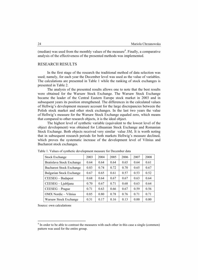
In the first stage of the research the traditional method of data selection was used; namely, for each year the December level was used as the value of variables. The calculations are presented in Table 1 while the ranking of stock exchanges is presented in Table 2.

The analysis of the presented results allows one to note that the best results were obtained for the Warsaw Stock Exchange. The Warsaw Stock Exchange became the leader of the Central Eastern Europe stock market in 2003 and in subsequent years its position strengthened. The differences in the calculated values of Hellwig’s development measure account for the large discrepancies between the Polish stock market and other stock exchanges. In the last two years the value of Hellwig’s measure for the Warsaw Stock Exchange equaled zero, which means that compared to other research objects, it is the ideal object.

The highest level of synthetic variable (equivalent to the lowest level of the object development) was obtained for Lithuanian Stock Exchange and Romanian Stock Exchange. Both objects received very similar value SMi. It is worth noting that in subsequent research periods for both markets Hellwig’s measure declined, which proves the systematic increase of the development level of Vilnius and Bucharest stock exchanges.

Table 1. Values of synthetic development measure for December data

Stock Exchange 2003 2004 2005 2006 2007 2008 Bratislava Stock Exchange 0.64 0.64 0.64 0.65 0.64 0.61 Bucharest Stock Exchange 0.83 0.74 0.72 0.70 0.65 0.67 Bulgarian Stock Exchange 0.67 0.65 0.61 0.57 0.53 0.52 CEESEG – Budapest 0.68 0.64 0.67 0.67 0.63 0.64 CEESEG – Ljubljana 0.70 0.67 0.71 0.68 0.63 0.64 CEESEG – Prague 0.71 0.63 0.66 0.67 0.59 0.56 OMX Nordic – Vilnius 0.85 0.80 0.78 0.76 0.71 0.71 Warsaw Stock Exchange 0.31 0.17 0.16 0.13 0.00 0.00

Source: own calculations

4 In order to be able to contrast the measures with each other in this case a single (common) pattern was used for the entire group.


Table 2. Ranking of stock exchanges based on the value of synthetic development measure

Stock Exchange 2003 2004 2005 2006 2007 2008 Bratislava Stock Exchange 2 3 3 3 6 4 Bucharest Stock Exchange 7 7 7 7 7 7 Bulgarian Stock Exchange 3 5 2 2 2 2 CEESEG – Budapest 4 4 5 4 5 5 CEESEG – Ljubljana 5 6 6 6 4 6 CEESEG – Prague 6 2 4 5 3 3 OMX Nordic – Vilnius 8 8 8 8 8 8 Warsaw Stock Exchange 1 1 1 1 1 1


In the second stage of the research a comparative study was conducted. This time, however, the method of selecting data for the analysis was modified. The synthetic development measure by Hellwig calculated using this method included all available data (namely, monthly values for each variable). The research results are presented in Tables 3 and 4.

Table 3. Values of synthetic development measure for monthly data

Stock Exchange 2003 2004 2005 2006 2007 2008 Bratislava Stock Exchange 0.75 0.77 0.77 0.77 0.79 0.80 Bucharest Stock Exchange 0.89 0.85 0.83 0.81 0.81 0.83 Bulgarian Stock Exchange 0.80 0.77 0.78 0.76 0.74 0.73 CEESEG – Budapest 0.78 0.73 0.76 0.78 0.79 0.80 CEESEG – Ljubljana 0.79 0.74 0.81 0.81 0.80 0.81 CEESEG – Prague 0.80 0.72 0.76 0.77 0.78 0.74 OMX Nordic - Vilnius 0.92 0.88 0.90 0.88 0.87 0.88 Warsaw Stock Exchange 0.57 0.50 0.49 0.47 0.47 0.49


Analyzing the presented results one may note the significant increase of Hellwig’s measure level for the researched market. At the same time, the gap between the weakest markets and the best of the selected objects – the Warsaw market - narrowed. Likewise, as was the case previously, the weakest markets (from the viewpoint of the analyzed information) were the Vilnus Stock Exchange and Bucharest Stock Exchange. In the second ranking, the position of the markets from the middle part of the list. The stock exchanges in Budapest, Ljubljana and Prague slightly changed their position by moving one place up or down on the list.


In addition, it is worth pointing out that the greatest gap between the selected values of Hellwig’s value measures for both rankings was noted between 2007 and 2008 (the final period of boom and beginning of decline in the market) and the global financial crisis.

Table 4. Ranking of stock exchanges based on the value of synthetic development measure

Stock Exchange 2003 2004 2005 2006 2007 2008 Bratislava Stock Exchange 2 5 4 3 5 4 Bucharest Stock Exchange 7 7 7 7 7 7 Bulgarian Stock Exchange 5 6 5 2 2 2 CEESEG – Budapest 3 3 3 5 4 5 CEESEG – Ljubljana 4 4 6 6 6 6 CEESEG – Prague 6 2 2 4 3 3 OMX Nordic - Vilnius 8 8 8 8 8 8 Warsaw Stock Exchange 1 1 1 1 1 1


In the third stage of the research Hellwig’s synthetic measure of development was calculated separately for each month. Next, for all selected values of the synthetic variable the median was determined, which was assigned as SMi value for a given year. The results of this stage are presented in Tables 5 and 6.

Table 5. Values of synthetic development measure for monthly SMi medians

Stock Exchange 2003 2004 2005 2006 2007 2008 Bratislava Stock Exchange 0.56 0.65 0.64 0.63 0.65 0.62 Bucharest Stock Exchange 0.77 0.80 0.73 0.69 0.67 0.66 Bulgarian Stock Exchange 0.88 0.67 0.62 0.58 0.56 0.53 CEESEG – Budapest 0.65 0.67 0.66 0.66 0.65 0.63 CEESEG – Ljubljana 0.68 0.68 0.71 0.68 0.66 0.64 CEESEG – Prague 0.67 0.65 0.65 0.65 0.66 0.58 OMX Nordic - Vilnius 0.80 0.85 0.81 0.76 0.73 0.71 Warsaw Stock Exchange 0.33 0.27 0.19 0.11 0.07 0.00


As in the case of the previous analyses the first place among the researched objects was given to the Warsaw Stock Exchange and the Vilnius and Bucharest stock exchanges remained in the last positions. The markets with average level of development (positioned in the center) had similar positions than previously.


Table 6. Ranking of stock exchanges based on the median of monthly values of synthetic development measure

Stock Exchange 2003 2004 2005 2006 2007 2008 Bratislava Stock Exchange 2 3 3 3 3 4 Bucharest Stock Exchange 6 7 7 7 7 7 Bulgarian Stock Exchange 8 5 2 2 2 2 CEESEG – Budapest 3 4 5 5 4 5 CEESEG – Ljubljana 5 6 6 6 6 6 CEESEG – Prague 4 2 4 4 5 3 OMX Nordic - Vilnius 7 8 8 8 8 8 Warsaw Stock Exchange 1 1 1 1 1 1


Undoubtedly, a great advantage of the third method is the ability to analyze the development of each of the researched stock markets on a month to month basis. The sample graphic presentation of the monthly valued SMi in 2003 clearly indicates the discrepancies between the levels of the synthetic variable (compare Figure 1).

The analysis of the SMi value allows one to note that Bulgarian Stock Exchange during the first eleven months of 2003 was the weakest of the analyzed stock exchanges. However, in the last month its development level significantly increased. Consequently, the stock exchange in Sophia ranked third in December (compare method 1)

The results presented in Figure 1 indicate a significant resemblance of the Ljubljana, Prague and Budapest stock exchanges5. The graphic presentation of the results confirms the major difference in the level of development between the Warsaw Stock Exchange and other exchanges.

The joint comparative analysis (compare Table 7 and Table 8) of all the obtained results indicates a clear disproportion in the calculated values of the synthetic development measure. In 2003 the greatest difference was noted for Bulgarian stock exchange, which in subsequent rankings ranked third, fifth and then eighth. In 2004 Slovakian and Slovenian stock exchanges moved by two places. A major difference in positioning was noted in 2005 for Czech stock exchange while in 2007 the Czech and Slovakian stock exchanges moved by two places depending of the presented method.

5 The similarity between these stock exchanges is not accidental. Beginning in 2009 each of them along with the Vienna Stock Exchange is a member of Central Eastern Europe Stock Exchange Group.


Figure 1. Monthly values for Synthetic Development Measure in 2003

0,200,300,400,500,600,700,800,901,00

1 2 3 4 5 6 7 8 9 10 11 12

Bratislava Stock Exchange Bucharest Stock ExchangeBulgarian Stock Exchange CEESEG - BudapestCEESEG - Ljubljana CEESEG - PragueOMX Nordic - Vilnius Warsaw Stock Exchange

Source: own work

For the remaining stock exchanges no significant changes were noted. The objects moved one place up or down in single cases. It is worth noting that the stock exchanges whose development significantly differed from the others usually held the same position in every ranking (Warsaw, Vilnius and Bucharest Stock Exchanges). Analyzing the positioning of the objects in the rankings one may note that the greatest number of changes was noted in the third ranking (compared to the other rankings).

CONCLUSION

In the conducted study the Warsaw Stock Exchange is the best stock exchange (from the point of view of the assigned criterion). The exchange ranked highest throughout all the consecutive years. The results are confirmed in the literature. The Warsaw Stock Exchange as the only stock exchange in the analysis is included in the average-class stock exchanges and is compared to the Vienna Stock Exchange ([compare Ziarko-Siwek 2008]). The weakest (the least developed stock exchanges from the view point of the assigned criteria) are the Vilnius and Bucharest stock exchanges.

As a result of implementing three distinct methods of calculating the synthetic measure of development. significant differences in the ranking were achieved. Analyzing the obtained results it seems justifiable to include partial data from sub-periods in the longer period (the second and third method of selecting data presented in the article). In case of major changes of an occurrence this may have a significant impact on the conducted analysis.


It is worth remembering that the second method (selection of all possible data) is connected with a certain risk. namely a large number of diagnostic variables.

According to [Zeliaś 2002] the number of diagnostic variables should be reduced since having too many variables may disturb or even block effective classification of objects. Therefore. the third method of data selection is recommended (to calculate the synthetic measure of each sub-period individually and then determine the correct average based on the analyzed occurrence). This will allow for including partial alterations of an occurrence and without increasing the number of diagnostic variables.

REFERENCES

Bartosiewicz S. (1976) Propozycja metody tworzenia zmiennych syntetycznych. Prace AE we Wrocławiu 84. Wrocław.

Cieślak M. (1874) Taksonomiczna procedura prognozowania rozwoju gospodarczego i określenia potrzeb na kadry kwalifikowane. Przegląd Statystyczny 21.1.

Hellwig Z. (1968) Zastosowanie metody taksonomicznej do typologicznego podziału krajów ze względu na poziom rozwoju oraz zasoby i strukturę wykwalifikowanych kadr. Przegląd Statystyczny 15.4.

Majewska A. (2004) Wykorzystanie metod klasyfikacji do określenia pozycji giełd terminowych na świecie. Prace Naukowe Akademii Ekonomicznej we Wrocławiu nr 1022 s.155-163.

Strahl D. (1978) Propozycja konstrukcji miary syntetycznej. Przegląd Statystyczny 25.2. Zeliaś A. (2002) Some Notes on the Selection of Normalization of Diagnostic Variables.

Statistics in Transition. Vol. 5 Nr 5. 784-802. Ziarko-Siwek U. (red.) (2008) Giełdy kapitałowe w Europie. Wydawnictwo Fachowe

CeDeWu. Warszawa.


COMPARISON OF THE BEEF PRICES IN SELECTED COUNTRIES OF THE EUROPEAN UNION

Stanisław Jaworski Department of Econometrics and Statistics


Abstract: Functional data analysis is used to examine beef price differences in selected countries of the European Union from 2006 to 2011. The prices are modeled as functional observations. The analysis is conducted in three steps relating to three kinds of functional data analysis. First the observations are smoothed with roughness penalty. Then functional principal analysis is applied. Finally functional analysis of variance is used to reveal significant difference between two given groups of countries.

Keywords: B-splines basis system, functional principal component analysis, functional analysis of variance, permutation tests

INTRODUCTION

The goal of the paper is to compare beef prices in European countries since 2006 to 2011. The price data are collected monthly and come from the website of Ministry of Agricultural and Rural Development (http://www.minrol.gov.pl). The main characteristic of the prices is that they don’t change rapidly. Two consecutive prices are unlikely to be too different from each other, so it seems reasonable to turn the raw price data into smooth functions and think of the observed data as single entities, rather than as a sequence of individual observations. A linear combinations of basis functions is used as a method for representing smooth functions. The basis function approach is designed to reveal the most important type of variation from the smoothed prices. A key technique in the approach is a functional principal component analysis.

The particular aim of the paper is to find out if there is a significant difference between beef prices considering old and new members of the European

32 Stanisław Jaworski

Union. In that case dependent variable is modeled as a functional observation so the methodology needed is a functional analysis of variance.

It is assumed that the first group, referring to the old members, consists of Belgium, Denmark, Germany, Greece, France, Spain, Ireland, Italy, Luxemburg, Nederland, Austria, Portugal, Finland, Sweden and United Kingdom. The second group of the new members consists of Czech Republic, Estonia, Latvia, Lithuania, Poland, Slovenia and Slovakia.

METHODS

It is assumed that the beef price ijy in time jt related do the i-th country has the form Njtxy ijjiij ,,2,1,)( …=+= ε (1)

where ijε is an unspecified random error and ∑=

=K

ikiki tctx

1)()( φ is a smoothed

price expressed as a linear combination of B - splines basis system kφ (see

Ramsay, Hooker, Graves (2009), p. 35). The coefficients ikc of the expansion are determined by minimizing, for each i , the least squares criterion

[ ] dssxDtxy ijiij ∫∑ +−222 )())(( λ (2)

Details of this approach can be found in Ramsey and Silverman (2005). The parameterλ is fixed. It can be selected arbitrarily or by minimizing Generalized Cross-Validation (GCV) measure (see Ramsay and Silverman (2005), p.97).

The smoothed prices are used in a functional principal component analysis (see Besse and Ramsey (1986), Ramsey and Dalzell (1991) and Besse, Cardot and Ferraty (1997)). In the analysis the weight functions Kξξξ ,,, 21 … are chosen consecutively. Each consecutive weight function mξ maximize

( )2

1)()(1∑ ∫

=

n

iim dssxs

nξ (3)

subject to

∫ = 0)()( dsss mk ξξ and (for mk < ) (4)

The vector ),,,( 21 nmmmm ffff …= where ∫= dssxsf imim )()(ξ , ni ,,2,1 …= ,

is called the m-th principal component. The percentage of variability of the first m components is expressed as

Comparison of the beef prices … 33

%100

1 1

2

1 1

2

∑∑

∑∑

= =

= =K

j

n

iij

m

j

n

iij

f

f (5)

The difference between beef prices for considered groups is investigated by functional analysis of variance. In formal terms, we have a number of countries in each group 2=g , and the model for the m th price function in the g th group, indicated by mgPrice , is

)()()()(Price tttt mggmg εαμ ++= . (6)

The function μ is the grand mean function, and therefore indicates the average mean price profile across all of countries. The terms gα are the specific effects on price of being in group g . It is required that they satisfy the following constraint ∑ =

gg t 0)(α for all t (7)

The residual function mgε is the unexplained variation specific to the m th price within group g .

As in ordinary analysis of variance F-ratio and t-test statistics can be calculated. Let denote them as )(tF and )(tT accordingly. These statistics can be used point-wise but it is desired to account for significant difference at different times. So the following statistics can be considered: )(sup tFF

t= and |)(|sup tTT

t= (8)

A permutation-based significance value can obtained for these statistics.

DATA ANALYSIS AND RESULTS

In this chapter the European mean beef prices are considered. The following countries are taken into account: Belgium (BE), Czech Republic (CZ), Denmark (DK), Germany (DE), Estonia (EST), Greece (GR), Spain (SP), France (FR), Ireland (IE), Italy (IT), Latvia (LV), Lithuania (LT), Luxembourg (LU), Netherlands (NL), Austria (AT), Poland (PL), Portugal (PT), Slovenia (SI), Slovakia (SK), Finland (FI), Sweden (SE), United Kingdom (UK). The beef prices are presented in Figure 1.


Figure 1. Beef prices in selected countries

Source: own preparation

The data were smoothed with B-splines system with roughness penalty parameter 1=λ . The choice of the parameter’s value was based on generalized cross-validation plot (Figure 2).

Figure 2. GCV plot

.Source: own preparation

The generalized cross-validation measure (GCV) is popular in the spline smoothing literature and was developed by Craven and Wahba (1979). The criterion is usually expressed as

( ) ( )⎟⎟⎠⎞

⎜⎜⎝

⎛−⎟⎟

⎠

⎞⎜⎜⎝

⎛−

=λλ

λdfn

SSEdfnnGCV )( (9)


where SSE is a sum of squared errors and ( )λdf is a degrees of freedom for a spline smooth. Figure 2 shows the variation of the generalized cross-validation statistic GCV (that is ∑=

iiGCVGCV )()( λλ , where index i relates to ix ) over

a range of log10(λ) values The generalized cross validation measure is minimized at 1.0=λ and it is

slightly higher for 1=λ . The bigger value was chosen because GCV criterion yields under-smoothing (see C.Gu (2002))

Next the smoothed data were explored by functional principal components analysis. The first two principal components account for 95% of the total variation.

A method found to be helpful in interpreting the components is to examine

plots of the overall mean function ∑=

=n

ii tx

nt

1)(1)(μ

and the functions obtained

by adding and subtracting a suitable component functions: 2,1, =±∧

mC mmξμ ,

where ∑=i

imm fn

C 21 . Figures 3 and 4 show such plots of the price data. In each

case the solid curve is the overall mean price and the other two curves clarify the effect of a given principal component. The effect of the first principal component of variation (covering 92% of the total variation) means that the greatest variability between countries corresponds to variability of its average beef price levels. As can be seen from the plot in Figure 3 this source of variability represents countries where, between 2006 and 2011, prices are at either low or high level. The i-th country for which the score 1if is high have much higher than average beef prices.

Figure 3. The first principal component curves



The second source of variation (Figure 4) is more complicated then the first one. It corresponds to countries where beef prices changed its relative level three times since 2006. This source of variation covers merely 3% of total variation.

Figure 4. The second principal component curves


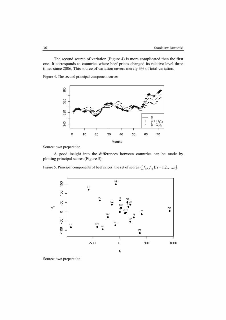
A good insight into the differences between countries can be made by plotting principal scores (Figure 5).

Figure 5. Principal components of beef prices: the set of scores ( ) niff ii ,,2,1:, 21 …= .



Majority of former members of Eastern Bloc are placed to the left side of the plot. It means that the countries have low beef prices since 2006. Opposite side of the plot relates to the countries with high beef prices in the period, for example to Greece, Italy and Portugal.

The conclusions drawn from principal component analysis mean that there can be a significant difference between beef prices with respect to if a country is an old or new member of European Union. Functional analysis of variance model is used in the paper to confirm this supposition. Estimated parameters: 21,, ααμ and prediction are presented in Figure 6.

The estimate of 1α is negative. It suggests that the new members have lower beef prices then the old ones. Although the parameter is changing over time the prediction plot in Figure 6 suggests that the difference between the two groups is relatively constant. The hypothesis that 1α is equal to zero was verified by permutation test. It is presented in Figure 7. The dashed line gives the permutation 0.05 critical value for the T - statistic and the dotted curve the permutation critical value for the point-wise T(t) - statistic

The test confirmed that there was a statistically significant difference between beef prices for the two considered groups.

Figure 6. Parameters and prediction of functional analysis of variance model



Figure 7. Permutation -based significance values for )(tT and T statistics


SUMMARY

Some features of mean beef prices across European countries were uncovered with functional data analysis. The most important type of beef price variations was revealed with help of smoothing techniques and functional component analysis. The difference between two separated groups of countries was investigated in terms of functional analysis of variance and permutation tests.

Some conclusions can be drawn. Apart from the overhead beef price in Europe increased since 2006 the source of the greatest beef price variability didn’t change over the investigated time (see Figure 3). The new members of European Union have still lower beef prices than the old ones. The difference is relatively constant as can be seen from prediction plot in Figure 6. It is interesting to note that such countries as Latvia, Lithuania, Estonia, where the beef prices are at low level (see Figure 5), are not the eurozone member states and the countries with high level of beef prices, for example Greece, Italy and Portugal, are highly indebted now. It means that it would be interesting to involve more explanatory variables for the price data analysis and provide more sophisticated model of functional regression then the presented functional variance model.


REFERENCES

Besse P.C., Cardot H. and Ferraty F. (1997) Simultaneous nonparametric regressions of unbalanced longitudinal data. Computational Statistics and Data Analysis, Vol. 24, 255-270.

Besse P.; Ramsay J.O. (1986) Principal components analysis of sampled functions. Psychometrika, 51, 285-311.

Craven, P. and Wahba, G. (1979) Smoothing noisy data with spline functions: estimating the correct degree of smoothing by the method of generalized cross-validation, Numerische Mathematik, 31, 377-403.

Gu, C. (2002) Smoothing Spline ANOVA Models”, Springer. Ramsay J.O, Dalzell C.J (1991) Some tools for functional data analysis (with discussion).

Journal of the Royal Statistical Society, Series B, 53:539-572. Ramsay J.O, Silverman B. W. (2005) Functional Data Analysis. Second Edition, Springer,

NY. Ramsay J.O, Hooker G., Graves S. (2009) Functional Data Analysis with R and MATLAB.

Springer.


UNEMPLOYMENT RATE FOR VARIOUS COUNTRIES SINCE 2005 TO 2012:

COMPARISON OF ITS LEVEL AND PACE USING FUNCTIONAL PRINCIPAL COMPONENT ANALYSIS

Stanisław Jaworski Department of Econometrics and Statistics


Konrad Furmańczyk Department of Applied Mathematics


Abstract: We apply the functional principal component analysis to compare the unemployment rate in euro area, Japan and USA since 2005 to 2012. For preprocessing analysis we used B-splines system with roughness penalty for smoothing the data. The analysis enables to reveal the most important type of variation in unemployment rate and its pace's in examined countries.

Keywords: B-splines basis system, functional principal component analysis, unemployment rate

INTRODUCTION

The unemployment rate is an important indicator with both social and economic dimensions. The time series analysis of unemployment are used by public institutions and the medias as an economic indicator. The banks may use this data for business cycle analysis. The general public might also be interested in changes in unemployment rate. Rising unemployment rate makes an increased pressure on the governments in order to spend on social benefits and cause a reduction in tax revenue. Rapid increase of unemployment rate may be a symptom of crisis in economy but its fixed decrease may be a signal for grown in the economy (for more information see . E. Burgen et al. (2012)).

Unemployment rate for various countries … 41

In the paper we analyze seasonally adjusted monthly unemployment rate in various countries from 2005 to 2012 for euro area, USA and Japan. The source of the data is the EUROSTAT report (see ec.europa.eu/eurostat). The unemployment rate is considered as a benchmark to ensure comparability of conditions of world economy. Although we should be aware of the definitional and technical pitfalls involved in the preparation of several unemployment series emanating from different sources of various countries.

Thus we expect the interpretability of the data comes not only from inspecting the level of the unemployment rate but also from the pace of the rate. Thus the great emphasis should be placed on getting sensible and stable estimation of pace. For this reason we decided to smooth the series by regular functions, possessing one or more derivatives.

In the chapter Methods we shortly described some mathematical tools and then in next chapter the conclusions were drown. Necessary computations were carried out by fda R package (see www.r-project.org ).

METHODS

We assumed that unemployment rate in the i-th country is of the form

Njtxy ijjiij ,,2,1,)( …=+= ε

where ∑=

=K

ikiki tctx

1)()( φ and kφ is B - splines basis system (see E.W.

Weisstein) and ijε is an unspecified random error. We used the penalized sum o squared errors fitting criterion to estimate

)(txi , that is we minimized

[ ] dssxDtxy ijiij ∫∑ +−222 )())(( λ

with respect to coefficients ikc . Details of this approach can be found in Ramsey an Silverman (2005). The smoothing parameter λ measures the rate of exchange between fit to the data in the first term and variability of the function x in the second term. For small λ the curve x tends to become more and more variable since there is less and less penalty on its roughness. In practice we chose parameterλ minimizing Generalized Cross-Validation (GCV) measure with respect to λ . (see Ramsey and Silverman (2005), p.97). After smoothing the data we carry out functional principal component analysis. This approach was taken by Besse and Ramsey (1986), Ramsey and Dalzell (1991)

42 Stanisław Jaworski, Konrad Furmańczyk

and Besse, Cardot and Ferraty (1997). Functional principal analysis can be defined as the search for a probe that reveals the most important type of variation in data.

In the first step we search function 1ξ which maximize sample variance

( )2

11

1

21 )()(11 ∑ ∫∑

==

=n

ii

n

ii dssxs

nf

nξ

subject to

.1)(21 =∫ dssξ

In the second step we find 2ξ such that ∫ = 0)()( 21 dsss ξξ and 2ξ maximize

( )2

12

1

22 )()(11 ∑ ∫∑

==

=n

ii

n

ii dssxs

nf

nξ

subject to

.1)(22 =∫ dssξ

Next, in m-step we find mξ such ∫ = 0)()( dsss mk ξξ for mk < and

maximize

( )2

11

2 )()(11 ∑ ∫∑==

=n

iim

n

iim dssxs

nf

nξ

subject to .1)(2 =∫ dssmξ

Very often the data are presented as a points in the graph in the first two principal components . , 21 ξξ In this case the criterion of quality of functional principal components has the form

%100

1 1

2

2

1 1

2

∑∑

∑∑

= =

= =K

j

n

iij

j

n

iij

f

f.

This formula compute percentage of variability of the first two principal components.

DATA ANALYSIS AND RESULTS

In this chapter we consider unemployment rate in Belgium, Bulgaria, Czech Republic, Denmark, Germany, Estonia, Ireland, Greece, Spain, France, Italy,


Cyprus, Latvia, Lithuania, Luxembourg, Hungary, Malta, Netherlands, Austria, Poland, Portugal, Romania, Slovenia, Slovakia, Finland, Sweden, United Kingdom, Norway, Croatia, Turkey, United States and Japan.

We used B-splines system and we have taken smoothing parameter 10=λ . The choice of the parameter’s value was based on generalized cross validation plot (Figure 1).

Figure 1. GCV plot.


The generalized cross validation measure is minimized at 1=λ and is slightly higher for 10=λ . We chose 10=λ to obtain more stable unemployment pace estimate then in the case for 1=λ . We found that the residual plots were quite good. Next the smoothed data were explored by functional principal components analysis. The first two principal components account for 92% of the total variation. They are presented in Figure 2 and Figure 3 as perturbations of the

mean unemployment rate, that is ∑=

=n

ii tx

nt

1

)(1)(μ is presented by solid line and

mmC ξμ±∧

, where n is the counts of countries, 2 ,1=m are presented by pluses and minuses. Constant mC is given by

.11

2∑=

=n

iimm f

nC

Observe (Figure 2) that the greatest variation between unemployment rate of various countries can be found since 2009 (from 40 month). Countries with high value of the first component relate to the countries with high unemployment rate.

The second large unemployment rate variation is explained by the second component (Figure 3). It expresses the difference between such countries like Ireland and Poland. The unemployment rate is relatively low in Ireland and high in Poland until 2009 and after the date the difference is opposite (Figure 4).


Figure 2. The first principal component as perturbations of the mean unemployment rate

Source: own preparation.

Figure 3. The second principal component as perturbation of the mean unemployment rate


Figure 4. Unemployment rate of Poland (dashed line) and Ireland (solid line)



A good insight into the differences between countries can be made by plotting principal scores (Figure 5). Norway, Netherlands, Austria and Japan are placed to the left side of the plot. It means that the countries have low unemployment rate. Opposite side of the plot relates to the countries with large unemployment rate. Spain is the special example of them.

Figure 5. Principal components of unemployment rate


Countries close to the top of the plot are able to cope with the unemployment since the crisis in 2008-2009 than the countries close to the bottom of the plot. The pace of unemployment rate in various countries was investigated in the paper by taking the first derivative of the smoothed unemployment rate series. Then functional principal component analysis was provided for the derived functions. The outcomes are visualized in Figures 6,7 and 8. It is seen that Estonia, Lithuania and Latvia were strongly influenced by the crisis and their unemployment rates extremely increased. These states quite good are managing with the problem of unemployment. It is encouraging that the growth in unemployment slowed there and became a decreasing. In contrast, in Greece, Bulgaria and Croatia the unemployment rate was higher and is increasing faster than in the rest of states.


Figure 6. First principal component as perturbations of the mean unemployment pace


Figure 7. Second principal component as perturbations of the mean unemployment pace


Figure 8. Principal components of unemployment pace



SUMMARY

Functional principal component analysis revealed the most important type of variation from the unemployment rates. The analysis gave us possibility to find out which states were the most influenced by the crisis and in which way. The 2008-2009 crisis highly separated states with respect to differences in unemployment rates but influenced them in different way. After the crisis a list of unemployment rates for various countries changed its order. Some states with high unemployment rate now have it at moderate level. Some states have dynamically growing unemployment rate. In the beginning of 2012 the difference in unemployment rates was high but what is promising it is a flattening of the dynamic of the unemployment rates.

REFERENCES

Besse P.C., Cardot H. and Ferraty F. (1997) Simultaneous nonparametric regressions of unbalanced longitudinal data. Computational Statistics and Data Analysis. Vol. 24, 255-270.

Besse P. Ramsay J.O. (1989) Principal components analysis of sampled functions, Psychometrika, 51, 285-311.

Burgen E., Meyer B. and Tasci M. (2012) An Elusive Relation between Unemployment and GDP Growth: Okun’s Law. Cleveland Federal Reserve Economic Trends.

Ramsay J.O. and Dalzell C.J. (1991) Some tools for functional data analysis (with discussion). Journal of the Royal Statistical Society Series B, 53:539-572.

Ramsey J.O. and Silverman B. W. (2005) Functional Data Analysis. Second Edition, Springer, NY.

Weisstein E.W. B-Spline. From MathWorld. A Wolfram Web Resource. http://mathworld.wolfram.com/B-Spline.html


COMPARISON OF CAPITAL MARKETS IN BULGARIA, ROMANIA AND SLOVAKIA IN YEARS 2001-2009

Krzysztof Kompa Department of Econometrics and Statistics


Abstract: The aim of research is evaluation of the development of stock exchanges in Sofia, Bucharest and Bratislava in the years 2000-2009. The analysis is provided for the logarithmic rates of return of main stock indexes quoted in the investigated countries, employing central tendency, dispersion and skewness measures as well as statistical inference. The research is provided for the whole period and for the sub-periods that are distinguished due to the general tendency at capital markets.

Keywords: emerging capital markets, stock index, time series analysis

INTRODUCTION

The Central and Eastern European countries have been undergoing transformation from a centrally planned economy to a market-orientated economic system since the collapse of the communist regimes in the year 1989. Privatization and activation of stock exchanges are ones of main symptoms of transformation. According to the level of capital markets development, countries in transition can be classified into four groups [Shostya et al. 2008]:

1. early reformers i.e. countries that activated stock exchanges in years 1989 – 1992: Slovenia (1989), Serbia (1989), Hungary (1990), Bulgaria (1991) Croatia (1991), Poland (1991), Slovakia (1991), and Czech Republic (1992);

2. laggards i.e. countries that activated stock exchanges in years 1993 – 1996: Kazakhstan (1993), Latvia (1993, Lithuania (1993), Kyrgyzstan (1994), Estonia (1995), FYR of Macedonia (1995), Moldova (1995), Romania (1995), and Russia (1995);

Development of capital markets in Bulgaria, Romania … 49

3. late reformers i.e. countries that activated stock exchanges in years 1998 – 2002: Belarus (1998), Georgia (1999), Azerbaijan (2000), Armenia (2001), and Ukraine (2002);

4. countries with no stock exchange: Albania, Bosnia & Herzegovina, Tajikistan, and Turkmenistan. However Tirana Stock Exchange1 together with Banja Luca and Sarajevo Stock Exchanges2 started quotations in 2002.

Among post-communist countries listed above, 10 of them became member states of European Union. Considering stock exchanges operated in these countries we notice that now we may select 3 groups of capital markets (Table 1).

Table 1. Groups of stock exchanges from transformed economies from EU states CEE Stock Exchange Group NASDAQ OMX Independent stock exchanges Prague Stock Exchange Tallinn Stock Exchange Warsaw Stock Exchange Budapest Stock Exchange Riga Stock Exchange Bratislava Stock Exchange Ljubljana Stock Exchange Vilnius Stock Exchange Bulgarian Stock Exchange Bucharest Stock Exchange

Source: own elaboration

In our research we consider only three stock exchanges located in Bratislava, Sofia and Bucharest since they are independent markets (together with the Warsaw Stock Exchange) among new EU states from that part of Europe. The aim of our investigation is to compare the development of stock exchanges in Sofia, Bucharest and Bratislava in the years 2000-2009. The analysis is provided for the logarithmic rates of return of main stock indexes quoted in the investigated countries, employing central tendency, dispersion and skewness measures as well as statistical inference. The research is provided for the whole period and for the sub-periods that are distinguished due to the general tendency at capital markets.

LITERATURE REVIEW

International market linkages has attracted investors and policy-makers attention. Consequently, international equity market integration is a topic often discussed in literature, especially many researchers have investigated the short-term and long-term interrelationships among worldwide financial markets. However Syriopoulos (2007) notices that despite the growing importance of the emerging Central European (CE) stock markets, the relevant body of research remains surprisingly limited. Furthermore, the empirical findings on this topic appear rather ambiguous and contradictory.

The paper [Gilmore et al. 2008] examines short- and long-term comovements between developed European Union (German and UK) stock

1 See http://www.tse.com.al 2 See http://www.bilberza.com, http://195.222.43.81/sase-final

50 Krzysztof Kompa

markets and three Central European (Poland, Czech Republic, Hungary) markets. While Gilmore and McManus (2002) are looking for links between three major CE markets (Poland, Czech Republic and Hungary), and the USA.

Voronkova (2004) investigates the existence of long-run relations between emerging Central European stock markets (Poland, Czech Rep. and Hungary), and the mature stock markets of Europe (Germany, France, UK) and US. Long-run linkages are detected between CE emerging and mature stock markets, implying limited diversification benefits for international investor portfolios allocated to these markets.

The paper [Syriopoulos, 2007] investigates the short- and long-run behavior of major emerging Central European (Poland, Czech Republic, Hungary and Slovakia) and developed (Germany and USA) stock markets and assesses the impact of the EMU on stock market linkages. The empirical findings have important implications for the effectiveness of domestic policy decision, as the emerging Central European states have recently joined the EU and local stock markets may become less immunized to external shocks.

MacDonald (2001) studies the CE stock market indices as a group against each of three developed markets (US, Germany and UK), and concludes significant long-run comovements for each of the groupings. Poghosyan (2009) assesses the degree of financial integration for Germany with eight transformed economies being “new” European Union member states.

Serwa and Bohl (2003) investigate contagion implications for European capital markets that are associated with seven important shocks between the years 1997 – 2000. The study uses correlation analysis and compares developed European markets (Greece, Germany, UK, France, Ireland, Spain and Portugal) with major Central and Eastern European (CEE) markets (Poland, Czech Rep. Russia and Hungary). Weak evidence of increased cross-market linkages following these crises is found, whereas emerging market returns do not converge to the developed market returns. CEE stock markets are concluded to still offer considerable risk diversification opportunities.

Egert and Kocenda (2005) investigate interrelations between three CE (represented by indexes BUX, PX-50 and WIG20) and Western European (- DAX, CAC, UKX) stock markets from the mid-2003 to the early 2005. They find signs of short-term spillover effects both in terms of stock returns and stock price volatility. The paper [Egert and Kocenda 2007] relates to analysis of comovements between three developed (France, Germany, UK) and three emerging (Czech Republic, Hungary, Poland) capital markets. Employing intraday data from June 2003 to January 2006 they find a strong correlation between German and French markets as well as between these two markets and the UK stock market. By contrast very little systematic positive correlation can be detected between mature and emerging European stock markets, and also within the latter group.

Analyses concerning relations among European emerging markets can be also found in [Shostya et al. 2008, 2009 and 2010], [Birg & Lucey 2006],


[Dubinskas & Stunguiene 2010], [Kompa & Witkowska, 2011], ], and [Witkowska et al. 2011], among others.

DESCRIPTION OF THE CAPITAL MARKETS

European emerging markets have been developing intensively however they still are considered as small and immature markets. It is worth mentioning that in September 2011 turnover of these capital markets (excluding Baltic market because they have been operate in frame of NASDAQ OMX Nordic group but it is very small market) was only 1.2% of total turnover in Federation of European Securities Exchanges (FESE) market. And among these seven stock exchanges 65.8% of turnover was made by the Warsaw Stock Exchange (Table 2).

Table 2. Percentage shares of traders and turnover observed in September 2011 Market Operator Trades Turnover Trades Turnover Stock index Bratislava Stock Exchange 0.04 0.04 0,90 2.66 SAX Bucharest Stock Exchange 3.65 1.40 89,36 89.11 BETC Bulgarian Stock Exchange 0.40 0.13 9,73 8.23 SOFIX Warsaw Stock Exchange 73.97 65.76 ∑ = 100.00 ∑ = 100.00 WIG CEESEG - Budapest 14.25 15.42 CEESEG - Ljubljana 0.38 0.57 CEESEG - Prague 7.31 16.68 Total 100.00 100.00 Source: own elaboration

Figure 1.Comparison of capitalization of analyses Stock Exchanges with Warsaw Stock Exchange In April 2011 [mln euro]

. Source: own elaboration

Comparison of capitalization of analyzed markets and the Warsaw Stock Exchange is presented at Figure 1. It is visible that Romanian Stock Exchange is

52 Krzysztof Kompa

the biggest capital market (among three investigated markets) since it’s share in turnover is over 89% Table 2. See also Figure 1 where it is visible that capitalization of all 3 markets is less than 17% of WSE, and capitalization of Stock Exchanges in Bucharest is 60.9%, Sofia - 23.7% and Bratislava - 15.3%.

Table 3. Characteristics of samples Sub- period Dates Type of the market Number of observations

BETC SAX SOFIX P0 1.01.2000 - 31.12.2009 whole 2609 2435 2260 P1 1.01.2000 - 8.10.2001 bear 461 432 2323 P2 9.10.2001 - 3.07.2003 stagnation 453 420 426 P3 4.07.2003 - 27.10.2005 bull 605 567 573 P4 28.10.2005 - 8.07.2007 bull 441 403 422 P5 9.07.2007 - 17.02.2009 bear 422 395 395 P6 18.02.2009 - 31.12.2009 bull 227 218 212 Source: own elaboration

Figure 2.Comparison of standardized plots of main stock indexes from analyzed capital markets


3 Quotations at Stock Exchange in Sofia starts from 20.10.2000.


In our investigation we consider main stock indexes that are listed in Table 2. Time spam of investigation is from 1.01.2000 to 31.12.2009. During this period we distinguish 6 sub-period that are defined due to the market tendency observed at the Warsaw Stock Exchange (see Table 3 and Figure 2). Note that sub-periods P3 and P4 are both bull markets but they are distinguished to have comparable numbers of observations in all samples. It is also visible that SAX – Bratislava Stock Exchange index has different tendency than three other indexes.

RESULTS OF EMPIRICAL ANALYSIS

In our investigation we consider logarithmic rates of return from the stock indexes daily quotations and analysis is provided applying: 1. daily expected returns from the participation units – y, 2. risk measures as: standard deviation - S, and variability coefficient – V, 3. measures of asymmetry - A and concentration – K, 4. statistical parametric tests for expected returns µj i.e. zero returns: H0: µj = 0 and

equality of two expected returns (obtained in different periods) i.e. H0: µj = µi, 5. statistical nonparametric tests for: normality - Kolmogorov-Lilliefors and

Jarque-Bera tests, and for randomness – runs test. Runs test together with identifications of so called weekday effects let us verify the Efficient Market Hypothesis [Fama 1970].

We also calculated the percentage share of positive and negative returns, as well as minimal (min) and maximal (max) values for each period and stock index that inform about the Stock Exchanges performance. All results are presented in tables where bold letters denote rejection of null hypothesis at the significance level 0.05.

Bucharest Stock Exchange

We start our analysis from the biggest market presenting basic characteristics of Romanian capital market in Table 4.

As one can see returns are significantly differ from zero in all sub-periods P1 – P6 (although not for the whole period P), and they are negative for bear markets. Variability is similar in all sub-periods though it is significantly bigger for the whole period. Time series seem to be symmetric but leptokurtic, also normality tests Jarque-Bera and Kolmogorov-Lilliefors shows that distribution of logarithmic returns is not normal. Runs test shows that in the whole sample P0, and the sub-periods P3 – P5 rates of return are not random that may suggest that the market was not efficient in Fama sense. We also analyze returns from quotations each day of the week i.e. Monday, Tuesday, etc. to check if there are weekday effects. But these returns do not significantly differ from zero and from each other (Table 5). Therefore we claim that weekday effect was not observed in all investigated periods.

54 Krzysztof Kompa

Table 4. Main characteristics of rate of returns: Bucharest Stock Exchange

Characteristics P0 P1 BEAR P2 P3

BULL P4.

BULL P5

BEAR P6

BULL Positive returns [%] 50.98 39.91 53.42 55.37 57.14 44.31 57.27

Negative returns [%] 47.60 58.57 42.60 44.13 41.95 54.74 42.29

Max 0.2307 0.2307 0.0929 0.0995 0.0732 0.1451 0.1312 Min -0.2604 -0.2604 -0.0584 -0.1048 -0.0636 -0.1577 -0.0809 Average - y 0.0003 -0.0024 0.0019 0.0022 0.0025 -0.0059 0.0047 Standard deviations 0.0233 0.0221 0.0139 0.0191 0.0167 0.0351 0.0305

V 77.2364 -9.3437 7.4105 8.7214 6.5881 -5.9873 6.5293 A -0.5541 -0.7353 0.7675 -0.2591 0.0050 -0.4728 0.0603 K 14.7585 66.9363 5.3784 5.2764 2.1964 2.9301 1.1811 Normality test J-B 23682.5 83656.2 570.55 689.67 84.46 159.77 11.75

Normality test K-L 0.47 0.48 0.48 0.47 0.48 0.46 0.47

Runs test -6.87 -1.74 -1.73 -5.25 -2.56 -2.71 -0.45 Source: own elaboration. Note: bold letters denote rejection of H0 at the significance level 0.05

Table 5. Values of test statistics for two expected values Tuesday Wednesday Thursday Friday Monday 1.096711 0.521209 0.591209 0.51908 Tuesday -0.65189 -0.48365 -0.63851Wednesday 0.115853 0.004196Thursday -0.11059

Source: own elaboration Note: bold letters denote rejection of H0 at the significance level 0.05

Bratislava Stock Exchange

However Bratislava Stock Exchange is the smallest one, among three being under consideration, we notice that it does not follow the trend that is observed on bigger markets. It is visible at Figure 2, and in rows describing percentage share of positive and negative returns. It is also confirmed by expected rates of returns since only the one from P3 period is significantly bigger than zero.


Table 6. Main characteristics of rate of returns: Bratislava Stock Exchange


BULL P4.

BULL P5

BEAR P6



Max 0.1188 0.0465 0.0596 0.0399 0.0407 0.0624 0.1188 Min. -0.0958 -0.0571 -0.0882 -0.0503 -0.0423 -0.0513 -0.0958

Average - y 0.0005 0.0011 0.0006 0.0019 -0.0002 -0.0005 -0.0010 Standard deviations 0.0123 0.0133 0.0151 0.0111 0.0090 0.0085 0.0173

V 23.9755 12.3302 24.7386 5.9713 -42.9343 -15.5351 -16.8215

A -0.1593 -0.0893 0.0736 -0.2734 -0.6032 -0.1898 -0.2571 K 10.7720 3.1731 5.1286 3.2236 5.3126 13.6223 18.1422 Normality test J-B 11712.4 174.09 442.84 244.55 479.08 2947.4 2805.1


Runs test -10.20 -2.49 0.84 -2.15 -2.55 -11.53 -9.77


Table 7. Values of test statistics for two expected values Tuesday Wednesday Thursday Friday Monday -0.45278 -1.27945 -1.88907 -1.937729Tuesday -0.89139 -1.56537 -1.62099 Wednesday -0.72336 -0.79417 Thursday -0.08107


Analyzed time series are not normally distributed and not random for all samples but the one for P2 period. Therefore one may suppose that the market is not efficient in Fama sense. In further investigation daily rates of return are put into order due to week days to check if weekday effects are observed in the samples. Due to results of the test H0: µj = 0 we claim that expected value of returns for Mondays, Tuesdays and Wednesdays do not differ significantly from zero while for Thursdays and Fridays they are significantly bigger than zero [Kompa 2011]. It is also visible that returns on Thursdays and Fridays are significantly bigger than on Mondays (Table 7).

56 Krzysztof Kompa

Bulgarian Stock Exchange

Looking at Table 8, we notice that rates of return in Bulgarian market significantly differed from zero in the periods denoted as P2 – P5. However the biggest variability was observed for the period P1 that is probably connected with the smal value of average returns in that period. Also for this Stock Exchange the distributions of returns are not notmal but series are not random only in selected periods, i.e.: P0, P3, P5 and P6.

Table 8. Main characteristics of rate of returns: Bulgarian Stock Exchange


BULL P4.

BULL P5

BEAR P6



Max 0.2107 0.2107 0.0839 0.0511 0.0353 0.0729 0.0631 Min. -0.2090 -0.2090 -0.1659 -0.0452 -0.0347 -0.1136 -0.0437 Average - y 0.0006 0.0003 0.0022 0.0019 0.0015 -0.0044 0.0022 Standard deviations 0.0197 0.0380 0.0211 0.0110 0.0076 0.0217 0.0174

V 30.7779 131.3518 9.4113 5.9343 5.2009 -4.9824 7.9257 A -0.5659 -0.0795 -0.9848 -0.0361 0.5777 -1.0339 0.7782 K 25.1261 13.0452 11.2341 3.1167 3.8239 4.0816 1.8520 Normality test J-B 57993.3 1538.9 2232.5 224.5 269.7 331.8 48.06


Runs test -5.73 -0.20 -0.67 -3.66 -1.81 -3.71 -2.89


Table 9. Values of test statistics for two expected values Tuesday Wednesday Thursday Friday Monday 0.374769 -1.38812 0.139348 -2.607635Tuesday -1.79046 -0.24377 -3.10579 Wednesday 1.563445 -1.03215 Thursday -2.85111



Rates of return significantly bigger than zero are observed only on Fridays, and they significantly differ from the ones obtained on Mondays, Tuesdays and Thursdays. Also returns on Wednesdays are significantly higher than returns on Tuesdays (Table 9).

CONCLUSIONS

Capital markets in European transformed economies are very small and immature with the exception of the Warsaw Stock Exchange, and this is the reason why the majority of Stock Exchanges in Central and Eastern and Southern Europe decided to unite and create bigger institutions as CEE Stock Exchange Group or to joint already existed stock market as NASDAQ OMX. As the result of such decisions now there are only four “independent” stock exchanges in transformed economies being state members of the European Union. Therefore in our analysis we consider Bratislava, Bulgarian and Bucharest Stock Exchanges. All analyzed stock exchanges are characterized by lack of efficiency in Fama sense.

Table 10. Values of test statistics for two expected returns Period Bucharest vs. Bulgarian Bucharest vs. Bratislava Bratislava vs. Bulgarian

P0 -0.49 -0.38 -0.21 P1 -1.00 -2.89 0.31 P2 -0.25 1.32 -1.27 P3 0.33 0.33 0.00 P4 1.14 2.96 -2.92 P5 -0.74 -3.07 3.33 P6 1.06 2.44 -1.91


Due to obtained results we may claim that both capital markets from Balkan region develop similarly while Bratislava Stock Exchange seems to differ from both Southern markets. That is visible in Table 10 which contains test statistics of for expected returns evaluated for pairs of Stock Exchanges. It is also proved that Bulgarian and Bucharest Stock Exchanges follow the market trends that are observed at Warsaw Stock Exchange while Slovak capital market seems not be affected by other markets.

REFERENCES

Birg G., Lucey B. M. (2006) Integration Of Smaller European Equity Markets : A Time-Varying Integration Score Analysis, IIIS Discussion Paper No.136, School of Business Studies and Institute for International Integration, University of Dublin, Trinity College, Dublin.

58 Krzysztof Kompa

Dubinskas, P., Stungurienė, S. (2010) Alterations in the financial markets of the Baltic countries and Russia in the period of economic downturn, Technological and Economic Development of Economy 16(3), pp. 502–515.

Egert B., Kocenda E. (2005) Contagion Across and Integration of Central and Eastern European Stock Markets: Evidence from Intraday Data, Working Paper No. 798, William Davidson Institute Working Papers Series from William Davidson Institute at the University of Michigan.

Egert B., Kocenda E. (2007) Time-Varying Comovements in Developed and Emerging Stock Markets: Evidence from Intraday Data, Working Paper No. 861, William Davidson Institute Working Papers Series from William Davidson Institute at the University of Michigan.

Fama E. F. (1970) Efficient Capital Markets: A Review of Theory and Empirical Work, Journal of Finance, pp. 383 – 417

Gilmore C. G., Lucey B. M., McManus G. M. (2008) The Dynamics of Central European Equity Market Comovements, The Quarterly Review of Economics and Finance, 48, pp. 605-622.

Gilmore C. G., McManus G. M.(2002) Internal Portfolio Diversification: US and Central European Equity Markets, Emerging Markets Review, 3, pp. 69-83

Kompa K. (2011) Development of Capital Markets in the Balkan Region, paper presented at 72-nd International Atlantic Economic Conference in Washington D.C.

Kompa K., Witkowska D. (2011) Capital Markets in the Baltic States in Years 2000–2010. Preliminary Investigation, in: Lacina, L.-Rozmahel, P. - Rusek, A. (eds.) Financial and Economic Crisis: Causes, Consequences and the Future. Bučovice: Martin Stříž Publishing, pp. 244 – 269.

MacDonald R. (2001) Transformation of External Shocks and Capital Market Integration, in M. Schroder (ed.), The New Capital Markets in Central and Eastern Europe, The Centre for European Economic Research, Springer Verlang, pp. 210-245.

Poghosyan T. (2009) Are “New” and “Old” EU Members Becoming More Financially Integrated. A Threshold Cointegration Analysis, International Economics and Economic Policy (Int. Econ. Econ Policy) 6, pp.259 – 281.

Serwa D., Bohl M. T. (2003) Financial Contagion: Empirical Evidence on Emerging European Capital Markets, Working Paper, N0. 5/03, European University Viadrina, Frankfurt.

Shostya A., Eubank Jr. A., Eubank III A. A. (2008) Diversification Potential of Market Indexes of Transition Countries, Working Paper presented at International Atlantic Economic Conference in Montreal.

Shostya A., Eubank Jr. A., Eubank III A. A. (2009) Risks and Returns of Market Indexes in Transition Countries, Working Paper presented at International Atlantic Economic Conference in Rome.

Shostya A., Eubank Jr. A., Eubank III A. A. (2010) Stock Returns in Transition and Developed Economies During the 2007 – 09 Financial Crisis, Working Paper presented at International Atlantic Economic Conference in Prague.

Syriopoulos T. (2007) Dynamic Linkages between Emerging European and Developed Stock Markets: Has the EMU any Impact?, International Review of Financial Analysis, 16, pp. 41-60.


Voronkova S. (2004) Equity Market Integration in Central European Emerging Markets: A Cointegration Analysis with Shifting Regimes, International Review of Financial Analysis 13, pp. 633-647.

Witkowska D., Kompa K., Matuszewska-Janica A. (2011) Analysis of Linkages between Central and Eastern European Capital Markets, Dynamic Econometric Models, Vol. 11 (forthcoming).


INDEX OF CENTRAL AND EAST EUROPEAN SECURITIES QUOTED AT WARSAW STOCK EXCHANGE - WIG-CEE

Krzysztof Kompa Department of Econometrics and Statistics


Abstract: After 20 years of transition in Central and Eastern Europe (CEE) the capital markets are considered to be emerging markets and they are still developing. In the last few years, the Warsaw Stock Exchange achieved the first position in the CEE region by the number of listed companies, the value of shares turnover and by the value of market capitalization. Because of the growing number of listed foreign companies from the CEE countries the Warsaw Stock Exchange decided to launch the first regional index. The aim of this paper is to describe the index construction and to investigate its properties through the application of statistical methods.

Keywords: emerging capital markets, stock index, WSE

INTRODUCTION

A stock market index is an aggregated measure of stock market dynamics. Such an index is computed from the prices of selected financial instruments (often as weighted average) and it is used to measure movements of the capital market [Blanchard, 1997, p.174]. We may distinguish different types of stock indexes such as price and total return stock indexes, volatility indexes, regional indexes, etc. The number of stock indexes that describe a certain stock exchange provides information about the capital market development.

There is a proliferation of stock market indexes. In recent years, the number of indexes developed by various providers has increased significantly. Numerous investment products are based on such indexes, as is the case for index funds (exchange-traded or not), structurized bonds, options and futures. Indexes are also used as benchmark portfolios by investment managers, both for asset allocation and performance measurement purposes [Amenc et al. 2006].

Index of CEE securities quoted at WSE: WIG-CEE 61

Globalization and integration have affected capital markets by allowing foreign companies to be listed at different markets, allow investors to invest abroad and construct their portfolio from different instruments that are issued or quoted in many countries. This creates demand for indexes that describe international or regional markets. Such indexes are constructed and listed by different institutions: stock exchanges, FTSE, HSBC Holding, MSCI and S&P among others.

Stock markets in Central and Eastern Europe (CEE) have been developing for over 20 years now but despite the growing importance of security exchanges in the region, the relevant body of research remains surprisingly limited [Syriopoulos 2007]. Therefore the aim of this research is to describe the construction of the index WIG-CEE, that provide information about the performance of foreign companies from the CEE region that are quoted on the Warsaw Stock Exchange, and to investigate the properties of this new index1. An analysis is provided for the logarithmic rates of return of the main stock indexes quoted in the reference countries, employing central tendency, dispersion and skewness measures as well as statistical inference and financial econometrics.

CENTRAL AND EAST EUROPEAN EXCHANGES

The transformation from a centrally planned economy to a market-oriented economic system in Central and Eastern Europe started in the year 1989. In 2004, eight post-communist countries together with Malta and Cyprus became members of the European Union, and two years later, two other states from the former Soviet bloc Bulgaria and Romania joined the EU. The creation of stock exchanges is one of the indications of transition, and it took place for the majority of these countries until 1995. However, some of the security exchanges were not established until 2002. It is worth mentioning that the development of each market has been implemented in different ways, independently from global trends and domestic economy. After twenty years of capital markets development in Central Europe the situation is as follows: • Baltic stock exchanges has joint already existed NASDAQ OMX; • Vienna together with Budapest, Ljubljana and Prague Stock Exchanges created

one regional alliance CEESEG; • Independent development of Stock Exchanges occurs in Slovakia, Bulgaria and

Romania; • Warsaw and Bulgaria Stock Exchanges became public listed companies.

According to the Federation of European Exchange (FESE) the Warsaw Stock Exchange (WSE) is the capital market in the CEE region with the highest number of listed companies. Between 2007 and 2011, the number of listed

1 The first presentation of the index idea took place in March 2012 [Kompa, Wiśniewski 2012], while the first quotation of the index, as a total return, took place on May, 30, 2012.

62 Krzysztof Kompa

companies increased twofold. In the same period the number of listed companies on the Prague and Vienna Exchanges decreased from 32 to 26 and from 119 to 105, respectively (Table 1). In addition, the market capitalization of the WSE has been the biggest in the CEE region since 2008, while the Vienna Stock Exchange lost its leadership in market capitalization of companies. However it still kept its first position by value of turnover until 2009 when the Warsaw market gained the first place in the region. It is possible to construct a taxonomic synthetic measure by taking into consideration the main factors of the CEE Stock Exchanges: number of company listed, markets’ capitalization and value of turnover. This measure confirms the leading role of WSE in the CEE region (Figure 1).

Table 1. Number of listed companies on main CEE Exchange Market Operator 2011 2010 2009 2008 2007Warsaw Stock Exchange 777 584 486 458 375CEESEG - Vienna 105 110 115 118 119CEESEG – Prague 26 27 25 29 32CEESEG – Budapest 54 52 47 43 41CEESEG - Ljubljana 66 72 76 84 87Bulgaria Stock Exchange 393 390 399 399 369Bratislava Stock Exchange 147 165 172 193 160

Source: Federation of European Exchanges

Figure 1. Taxonomy of CEE Stock Exchanges

Source: own computation from FESE Note: CEE-V denotes Vienna SE, CEE-P denotes

Prague SE, CEE-B denotes Budapest SE and CEE-L denotes Ljubljana SE

WARSAW STOCK EXCHANGE INDEXES

The Warsaw Stock Exchange was founded in 1991 as a joint stock company held solely by the Polish State Treasury. The mission of the WSE was to provide


an organized trading in financial instruments (equities, bonds, structured products, investment certificates and derivatives), to promote such trading and to disseminate market information. In 2010, WSE became a public company and its shares have been trading on the WSE Main List since November 9, 2010.

The Warsaw Stock Exchange conducts trading in financial instruments in four markets. The Main List has been in operation since the first trading day on April 16, 1991. Most of the instruments are traded here: equities, rights-to-shares, pre-emptive rights, as well as other equity-based instruments, bonds, futures contracts, option and others. NewConnect is a market organized and maintained by WSE as an alternative trading system. It was designed for startups and developing companies. The market was launched on August 30, 2007. Catalyst is a debt instruments market launched on September 30, 2009. Catalyst contains two different platforms for retail and wholesale customers. State Treasury, municipal, corporate and mortgage instruments are traded on this market. The Energy Market was launched on December 11, 2010. It is a transaction platform for energy deals and energy-related futures for all type of customers: producers, traders and users.

At the end of 2011 the market capitalization of companies listed on WSE was 450 billion PLN and the value of turnover of equities reached a historical high of 258 billion PLN. The volume of futures contracts turnover also reached a high of 13 million contracts traded.

The first foreign company – BACA bank was listed in October 2003 (dual listed on both the Warsaw and Vienna Stock Exchanges). In 2006 the WSE launched a new aggressive strategy focusing on the acquisition of new companies, domestic and foreign. As a result of this campaign, the number of foreign companies listed on all WSE markets increased from 20 in 2006 to 45 in 2011. Because of a rapidly growing number of companies of Ukraine domicile, a decision was made to launch the first index of foreign companies listed on WSE in 2011 - the WIG-Ukraine index.

Due to the steady development of the Warsaw Stock Exchange the number of stock indexes has been increasing systematically, providing a good description of the WSE markets. At present several groups of the main market indexes can be distinguished: • Total Index WIG, and total indexes for branches; • Price Blue Chip Index WIG20, and indexes for medium and small size

companies mWIG40 and sWIG80; • Index of domestic companies WIG Poland, and index of Ukrainian companies

WIG-Ukraine; • Indexes for investment strategies WIG20short and WIG20lev; • Index of companies that obey corporate governance rules RESPECT and that

pay dividend WIGdiv.

64 Krzysztof Kompa

Therefore, the next step was introduce a new index for the WSE that describes the performance of foreign companies from the CEE region that are listed on the Warsaw Stock Exchange: WIG-CEE.

WIG-CEE INDEX CONSTRUCTION

A stock index is generally a portfolio of stocks, bonds or other kinds of investments. Stock indexes are used to represent either segments and sectors of a stock exchange or the whole stocks traded on the exchange. One of the most common ways to understand a stock index is to look at the composition of the stocks it represents. Generally, the set of rules requires the stocks to satisfy certain criteria, such that [Broby 2011]: • All the investments in the index are subject to selection. • Includes calculations and rules for weighting of the index components. • Provides specific instructions for adjustments to maintain consistency.

According to the main assumption, the index contains companies from Bulgaria, Czech Republic, Estonia, Hungary, Latvia, Lithuania and Ukraine. The selection of companies for the index portfolio is based on two-level parallel analysis: country and company. A certain company and country is included in the index composition if the following criteria are fulfilled: • there are at least two companies from one country; • the companies should represent at least two different industry (branches)

according to the WSE Industry Classification; • the companies listed on the WSE should cover at least 10% of the whole market

capitalization • there must be at least 10% of shares in free float. Other WIG-CEE index criteria are similar to the main WSE indexes i.e.: • the index portfolio is based on the number of shares in free float; • only 50% of companies from each country listed on the WSE are admitted in

the index composition; • the weighting depends on the number of companies in the index portfolio i.e. if

the number of companies in the index composition is above 30 then the contribution of one company is limited to 10% and to 25% otherwise.

Periodic adjustments take place every quarter at the end of February, May, August and November when the new portfolio of the index is evaluated as a background to index changes after the third Friday of March, June, September and December. In the case of a merger, delisting or bankruptcy the company could be removed from the index portfolio and new company is added if there are other companies from the country of origin that fulfill the distinguished roles.


The general formula for the index calculation is as follows:

)0()(0

IAM

MtI

t

t=

where Mt , M0 - market value of index portfolio at date t and the base date, I(t), I(0),– index value at the date t and base date, At – adjustment coefficient.

The WIG-CEE index composition procedure is as follows: The free-float value of CEE securities quoted on the WSE and selected for

the WIG-CEE index - WIGCEEval - is defined as:

∑=

=+++=N

iiivNval pnpnpnpnWIGCEE

12211 ... ,

where N – number of securities in WIG-CEE index portfolio, ni - number of shares of i-th company in free-float, pi - market price of shares i; i = 1, 2, 3, …, N.

The weighting factor iω describing a part of the capitalization of one company relative to the value of the index portfolio is calculated as:

∑=

=N

iiiiii pnpn

1/ω

Let: maxmax, iii ωω = . In any case of relation between weight factor max,iω

and desired contribution Ω of one company in the index portfolio composition: Ω<max,iω or Ω>max,iω , factor max,iω is replaced (due to the index methodology)

by Ω: Ω=→= *max,max, max iiii ωωω and new weight factors *

iω are calculated

as: ii ωϕω ⋅=* , where the scale factor ϕ is defined as )1/()1( max,iωϕ −Ω−= .

Recursion of the full procedure occurs until εω <Ω−max *ii

. Therefore, the

final WIG-CEE index calculation formula is as follows:

∑=

=N

itiiit pnWIGCEE

1,

*ω

where *iω - scaled weights, in - number of shares of i-th company in the index

portfolio, tip , - market price of shares i at the trading day t; i = 1, 2, 3, …, N If adjustment of the WIG-CEE index is necessary, then after composition

of new portfolio for the date of adjustment Ti , the adjustment factor is calculated as:

)()()(

1 ii

iii TWIGCEE

TWIGCEET−

=ψ

66 Krzysztof Kompa

where WIGCEEi-1(Ti), WIGCEEi(Ti) – value at the day Ti of index portfolio composed before and after adjustment respectively, and the new WIG-CEE is listed until next adjustment event as:

],0[;)(

)()( 1 kikii

iii TTt

TtTWIGCEEtTWIGCEE +++ −∈+=+

ψ

where: Ti – day of implementation of adjusted index, t - every trading day between adjustment days i =1,2,3,…

EMPIRICAL ANALYSIS OF WIG-CEE INDEX

In our investigation we consider the main stock indexes for selected CEE countries i.e.: Poland – WIG, CEE Region (quoted at Vienna Stock Exchange) – CETOP20, Czech Republic – PX, Hungary – BUX, Bulgaria – SOFIX. The time span of the investigation is from 1.01.2011 to 31.12.2011. During this period we distinguish four periodical adjustments that are defined due to the WIG-CEE index specification. The lists of companies that are used for the index calculation at the beginning and the end of the year 2011 are presented in the Appendix (Tables A1 and A2) and the final plot of the WIG-CEE time series is given in Figure 2.

Figure 2. Plot of WIG-CEE, WIG & CETOP20 time series for the analyzed period

Source: own calculation


In our investigation, we want to recognize selected statistical properties of the proposed WIG-CEE index and compare it to other indexes from CEE Stock Exchanges. We consider the logarithmic rates of return from the stock indexes daily quotations:

)ln()ln( 1−−= ttt WIGCEEWIGCEEr and we apply daily expected returns from the participation units - yt; risk measures (- standard deviation - S, variability coefficient - V) and measures of asymmetry - A and concentration – K, as well as statistical parametric and nonparametric tests. Selected results are presented in the tables below where bold letters denote the rejection of the null hypothesis at the significance level 0.05.

The results in Table 2 indicate that all the indexes are very strong however, the logarithmic rates of return are strongly correlated with the regional index CETOP and BUX while it is less correlated with WIG, PX and SOFIX (Tab. 3)

Table 2. Indexes correlation table

WIG-CEE WIG CETOP BUX PX SOFIX WIG-CEE 1

n

uxy

xy

21 ρ

ρ

−=

WIG 0.9414285 1 CETOP 0.9518828 0.9827428 1 BUX 0.9524188 0.9733519 0.9751545 1PX 0.9625844 0.9703824 0.9917603 0.9686424 1 SOFIX 0.8482803 0.8675074 0.9053097 0.8412209 0.8919088 1

Source: own computation

Table 3. Logarithmic rates of return correlation table

WIG-CEE WIG CETOP BUX PX SOFIX WIG-CEE 1 H

0: ρ

xy=0

H1: ρ

xy>0

μα=μ

0,05 =2,575

WIG 0.6536972 1 CETOP 0.6263809 0.9074728 1 BUX 0.5473974 0.6975237 0.8236008 1PX 0.5454550 0.6748685 0.7756087 0.5554220 1 SOFIX 0.1605466 0.1589521 0.1532889 0.0829252 0.1991412 1


68 Krzysztof Kompa

The descriptive statistics (Table 4.) confirm similarity of behavior of logarithmic rates of return for analyzed indexes.

Table 4. Descriptive statistics of logarithmic rates of return for analyzed indexes Statistics WIG-CEE WIG CETOP BUX PX SOFIX

n 303 303 303 303 303 303 Min -0.06297358 -0.062436059 -0.079617-0.06984201 -0.061346 -0.04073 Max 0.068081575 0.04104653 0.0520295 0.055149170.0425934 0.036421 Mean -0.0352543 -0.03440151 -0.03691 -0.0333191 -0.03631 -0.0348 Std. Error 0. 03802722 0.03761359 0.039807 0.03936650.0007929 0.000583 Median -0.0346548 8.50915E-05 0 0 0 0 Std. Dev 0.01397291 0.013252893 0.017071 0.016304110.0138021 0.01015 Variance 0.03195242 0.03175639 0.032914 0.0326582 0.031905 0.03103 Kurtosis 4.33721072 4.017978897 2.6049766 2.113911762.4124816 1.991368 Skewness 0.111051945 -0.83275825 -0.588969-0.43754545 -0.487634 -0.02527 Volatility 26.5932389 30.10985129 24.705479 49.121593421.878849 21.22921 Spread 0.131055155 0.103482589 0.1316461 0.124991070.1039391 0.077155 Total -0.15920535 -0.133365867 -0.209367-0.10056971 -0.191145 -0.14488

Confidence level(95,0%) 0.001579636 0.00149824 0.0019299 0.001843180.0015603 0.001148

Source: own computation Note: 0,03 denotes 0,000

The results presented in Table 5 show that over the analyzed period the expected daily returns from all investigated indexes are significantly negative, the time series of daily rates of return are characterized by significant asymmetry and the probability distribution is not normal which is additionally confirmed by the Kolmogorov-Lilliefors and Jarque-Berra normality tests.

Table 5. Test statistics for daily rates of return

WIG-CEE WIG CETOP BUX PX SOFIX Mean value H0: E(r)=0; H1: E(r)<0 (mean value is significantly negative) U-statistics 0.65456093 0.578112958 0.70457631 0.354363407 0.7956038 0.8199501

Skewness Ho: A=0; H1: A<0 or A>0 U-statistics 0.789172346 5.917859269 4.18541339 3.109344616 3.46529091 0.1796122

Kurtosis Ho: K=0; H1: K>0 U-statistics 15.4108366 14.27655244 9.25591843 7.511082773 8.57195147 7.0756627



In Table 6 we compare the expected rates of return and variance of returns for each pair of indexes. It is noted that the expected returns from all indexes are the same since the null hypothesis about equality of two expected values cannot be rejected. However, some of indexes are characterized by a different risk that is denoted by bold letters.

Table 6. Test statistics for daily rates of return

Two means equality H0: E(ri)= E(rj); H1: E(ri) ≠ E(rj) WIG-CEE WIG CETOP BUX PX SOFIX

WIG-CEE x WIG 0.0770807 x

CETOP -0.1306285 -0,2020289 x BUX 0.1568769 0,0896715 0,2647736 x PX -0.0934260 -0,1734727 0,0476846 -0,2435874 x

SOFIX 0.0476681 -0,0396075 0,1865471 -0,1325277 0,1551516 x

Two variance equality H0: σi=σ

j; H1: σi

>σj F

kryt= 1.208766

WIG-CEE x WIG 1.1116068 x

CETOP 1.4926071 1.65919216 x BUX 1.3615122 1.51346617 1.0962863 x PX 0.97570649 1.08460197 1.529771 1.3954116 x

SOFIX 1.8949726 1.70471484 2.82845 2.5800282 1.848937 x


Another characteristic that is tested is the weak form of informational efficiency that is verified using Wald-Wolfowitz tests of 2-runs and 3-runs and McKinley variance ratio test together with the testing for the so called weekday effects employing daily and weekly rates of returns (Table 7 and 8).

70 Krzysztof Kompa

Table 7. Test statistics for weekday effects for daily logarithmic WIG-CEE rates of returns


Table 8. Test statistics for weekday effects - weekly logarithmic WIG-CEE rates of returns


None of the null hypotheses of all applied tests is rejected, except in some cases of variance of returns i.e. risk is different on Tuesdays for daily data and

H0: E(r)=0 H1: E(r)≠0

Mon Tue Wed Thu Fri -1.0214269 0.3133852 -0.1430307 -1.1432172 0.724936

Mea

ns e

qual

ity

Mon x Tue -0.0036744 x Wed -0.6576837 0.3037549 x Thu 0.0486789 1.1077494 0.7259947 x Fri -1.2389857 -0.4023868 -0.6235574 -1.3199403 x

Var

ianc

e eq

ualit

y

Mon x Tue 2.0613918 x Wed 0.8344243 1.7200753 x Thu 0.8919438 1.8386455 1.0689331 x Fri 0.9045226 1.8645755 1.0840081 1.0141028 x

N 61 61 61 60 60 Mean -0.0020183 0.0004313 -0.0002582 -0.0021511 0.0013737 Std. Dev 0.0154329 0.010749 0.0140975 0.0145753 0.0146777 Variance 0.0002382 0.0001155 0.0001987 0.0002124 0.0002154

H0: E(r)=0 H1: E(r)≠0

Mon Tue Wed Thu Fri -0,6524608 -0,7622185 -0,6857958 -0,7294278 -0,7516035

Mea

ns

equa

lity

Mon x Tue 0.1447402 x Wed 0.0964169 -0.043901 x Thu 0.1988478 -0.0069522 0.0363483 x Fri 0.1654522 -0.0876765 -0.0396791 -0.0786827 x

Var

ianc

e eq

ualit

y

Mon x Tue 1.3323742 x Wed 1.3861923 1.0403926 x Thu 1.3933674 1.0457778 1.0051762 x Fri 0.9859896 1.3513066 1.4058893 1.4131664 x

N 61 61 61 60 60 Mean -0,0020183 0.0004313 -0.0002582 -0.0021511 0.0013737 Std. Dev 0,0154329 0.010749 0.0140975 0.0145753 0.0146777 Variance 0,0002382 0.0001155 0.0001987 0.0002124 0.0002154


on Mondays and Fridays for weekly rates of return. Therefore, we are not allowed to reject the hypothesis about market efficiency in the Fama sense.

CONCLUSIONS

In this paper we discuss the construction and methodology of the index describing companies operating in the CEE that are listed on the Warsaw Stock Exchange – WIG-CEE. We also investigate the basic properties of the index and compare the generated WIG-CEE time series to quotations of the WIG, CETOP, BUX, PX and SOFIX indexes. In our opinion the presented index appropriately describe the CEE stocks quoted on the WSE and, since it has been quoted at the WSE since May, 2012, it can be used as a basic instrument for derivatives.

REFERENCES

Amenc, N. Goltz, F. Le Sourd, V. (2006). Assessing the Quality of Stock Market Indices. EDHEC Publication Lille-Nice.

Blanchard O. (1997) Macroeconomics, Prentice Hall, Upper Sadle River. Broby, D. P. (2007) A Guide to Equity Index Construction. Risk Books, London. Broby, D. (2011) Equity Index Construction, The Journal of Index Investing, Fall 2011.

Vol. 2, No. 2: pp. 36-39 Fama E. F. (1970) Efficient Capital Markets: A Review of Theory and Empirical Work,

Journal of Finance, pp. 383 – 417 Kompa, K. Wiśniewski T. (2012) The First Index of Warsaw Stock Exchange for Central

and East European Securities – WIG-CEE, paper presented at 73rd International Atlantic Economic Conference in Istanbul (draft under reviewing procedure).

Syriopoulos, T. (2007) Dynamic Linkages between Emerging European and Developed Stock Markets: Has the EMU any Impact?, International Review of Financial Analysis, 16, pp. 41-60.

72 Krzysztof Kompa

APPENDIX

Table A1. WIG-CEE Index Portfolios: Index portfolio at the beginning of 2011

No Company Country Share in index Value of package [PLN mill]

1 KERNEL Ukraine 25,00% 1 083 500 2 CEZ Czech Republic 25,00% 1 083 500 3 ASTARTA Ukraine 16,44% 712 685 4 PEGAS Czech Republic 12,91% 559 684 5 OLYMPIC Estonia 7,18% 311 156 6 FORTUNA Czech Republic 6,39% 276 822 7 AGROTON Ukraine 4,56% 197 617 8 SILVANO Estonia 1,64% 71 162 9 PHOTON Czech Republic 0,64% 27 556

10 BGSENERGY Czech Republic 0,24% 10 318


Table A2. WIG-CEE Index Portfolios: Index portfolio at the end of 2011

No.

Company Country Package

[PLN mill] Share in

index No Company Country

Package [PLN mill]

Share in index

1 ICPD BG 4,03 0,06% 14 AGROTON UKR 487,58 0,82%

2 SOPHARMA BG 718,08 1,46% 15 ASTARTA UKR 1600 3,78%

3 BGSENERGY CZ 32,55 0,06% 16 COALENERG UKR 1168,94 2,81%

4 CEZ CZ 11104,6 25,00% 17 IMCOMPANY UKR 327,09 0,59%

5 FORTUNA CZ 800,44 1,96% 18 KERNEL UKR 5613,7 23,16%

6 ICMVISION CZ 3,92 0,01% 19 KSGAGRO UKR 344,78 0,72%

7 PEGAS CZ 650,66 4,46% 20 MILKILAND UKR 562,5 0,95%

8 PHOTON CZ 38,18 0,08% 21 OVOSTAR UKR 572,7 0,01%

9 OLYMPIC EST 802,05 1,96% 22 SADOVAYA UKR 417,07 0,64%

10 SILVANO EST 552,61 1,11% 23 WESTAISIC UKR 187,57 1,82%

11 AGROWILL LT 62,77 1,07% 24 MOL HUN 11133,7 25,00%

12 AVIASG LT 214,46 0,87% 25 ESTAR HUN 382,8 1,58%

13 AGROLIGA UKR 23,04 0,02%



A RESEARCH NOTE: STATE BASED FACTORS AFFECTING

INWARD FDI EMPLOYMENT IN THE U.S. ECONOMY

Lucyna Kornecki Embry-Riddle Aeronautical University

Daytona Beach, FL [email protected] E. M. Ekanayake

Bethune-Cookman University Daytona Beach, FL

[email protected]

Abstract: This empirical research investigates state based factors affecting the inward FDI employment among fifty states of the United States, uses annual data for the period of time from 1997 to 2007 and identifies several state-specific determinants of FDI employment. The results indicate that the major factors exerting positive impact on inward US FDI employment are: real wages, infrastructure, unionization level, educational attainment, FDI stock and manufacturing density. In addition, the results show that gross state product growth rate, real per capita taxes and share of scientists and engineers have negative impact on FDI employment. Our findings indicate the importance of selected variables in evaluating the effects of FDI flow on state employment.

Keywords: employment, foreign direct investment (FDI)

INTRODUCTION

Foreign direct investment (FDI) plays an extraordinary and growing role in the global business and represents an integral part of the U.S. economy. The inward FDI constitutes important factor contributing to output growth and employment in the U.S. economy. The United States continues to be the leading destination for foreign direct investment (FDI) and the leading investor in other economies. Kearney’s index ranks World inward FDI and reveals FDI flows and the factors

74 Lucyna Kornecki, E. M. Ekanayake

that drive corporate decisions to invest abroad. The major finding in A.T. Kearney's 2010 FDI report indicates that China and United States are the most attractive FDI locations in the world and have achieved unprecedented levels of investor confidence. The United States remains a strong FDI magnet in the World economy. Recently, China, India, and Brazil made the top spots of Kearney’s FDI Confidence Index (http://www.atkearney.com/main.taf?p=5,3,1,140,1).

Foreign companies and their U.S. subsidiaries generate enormous economic benefits for the American economy and bring billions of investment dollars into the United States, create thousands of in- sourced American jobs, and highlight the importance of the U.S. market for foreign companies. The state development agencies have an established framework of financial incentives to influence the final business location decision. Typical state inducements may include: low-interest loans, reduced income, sales, or property tax liability and grants for training or infrastructure improvement (http://www.locationusa.com/UnitedStates GovernmentAssistance/jul08/state-agencies-business-investment-USA.shtml).

LITERATURE

The empirical literature related to the state based determinant of FDI employment in the U.S. is limited. In evaluating the effects of FDI on the local economies, economists focus primarily on the performance of foreign-owned subsidiaries operating in the U.S. It is already known that the establishment of a new foreign subsidiary or the expansion of an already existing one leads to higher employment and wages (Axarloglou, 2005). Reserchers identified link between job growth in the U.S. economy during a period of increasing foreign direct investment flow. The economic impact on U.S. employment due to FDI is evident, as are linkages among the various benefits due to the inward flow of FDI (Craig, 2008).

Acording to Axarloglou & Pournarakis in the last two decades, various US states offered strong economic incentives in an effort to attract FDI inflows, with the hope that FDI would stimulate local economies (Axarloglou & Pournarakis, 2005). Axarloglou, Casey and Han analyzed the effects of FDI inflows in local economies across US states. The empirical results point out that the US economy benefits from FDI inflows in manufacturing both in terms of employment and real wages. Overall, FDI inflows have a positive and in several cases statistically significant impact on local employment and wages. However, these effects vary across US states. In some states, such as California, Michigan, Ohio and Pennsylvania, FDI inflows appear to expand both employment and wages while in others, like Florida, Georgia and Virginia appear to depress both employment and wages. Finally, in several US states, such as in Connecticut, Delaware, Kentucky, and Louisiana, FDI inflows have mixed effects on local labor markets, with predominantly negative effects on local employment and expanding effects

A research note: State based factors … 75

on local wages. There is evidence that these results are due to the industry composition of FDI inflows across states. FDI inflows in Printing and Publishing, Fabricated Metals, Industrial Machinery and Transportation Equipment have positive employment and wages effects, while FDI inflows in Furniture and Leather have negative effects (Axarloglou, Casey & Han, 2006).

The studies by Borstorff, Collum and Newton relate to FDI in the southern U.S., specifically automobile FDI in Alabama and describe state-specific features of southern states in recruiting foreign investment bringing the employment opportunities (Borstorff, Collum & Newton, 2007).

Ajaga and Nunnen a analysis complements the regression analysis of Mullen and Williams and the Markov chain approach of Bode and Nunnenkamp and presents strong evidence of favorable FDI effects on output and employment at the level of US states (Ajaga & Nunnen, 2008).

Alfaro examined the effect of foreign direct investment on growth in the primary, manufacturing, and services sectors. Foreign direct investments in the primary sector, however, tend to have a negative effect on growth, while investment in manufacturing a positive one. Evidence from the service sector is ambiguous (Alfaro, 2003).

Blomstrom, Fors and Lipsey compared the relation between foreign affiliate production and parent employment in US manufacturing multinationals with that in Swedish firms. US multinationals allocated some of their more labor-intensive operations in developing countries, reducing the labor intensity in their home production. Swedish multinationals produce relatively little in developing countries and most of it in high-income countries, such as the United States and Europe associated with more employment, particularly blue-collar employment, in the parent companies (Blomstrom, Fors and Lipsey, 1997).

Bode and Nunnenkamp investigated the effects of inward FDI on per-capita income and growth of the US states since the mid-1970s. This study analyzed the long-run relationships between inward FDI and economic outcomes in terms of value added and employment at the level of US states (Bode & Nunnenkamp, 2007). The study found that employment-intensive FDI, concentrated in richer states, has been conducive to income growth, while capital-intensive FDI, concentrated in poorer states, has not.

DATA SOURCES AND VARIABLES

In order to test the implications of our models, we collected a panel of aggregate data on foreign direct investment on all U.S. states, excluding the District of Columbia. The entire data set includes 50 states for which foreign direct investment and all other relevant variables are reported over the 1997–2007 period.

In the United States, the Bureau of Economic Analysis (BEA), a section of the U.S. Department of Commerce, is responsible for collecting economic data related to FDI flows. Monitoring this data is very helpful in trying to determine the


impact of FDI on the overall economy, but is especially helpful in evaluating states and industry segments. The data on stock of FDI are from the U.S. Department of Commerce, Bureau of Economic Analysis (BEA).

The real per capita disposable income is measured as the nominal per capita disposable income deflated by the GDP deflator in constant (2000) U.S. dollars. The real per capita taxes is measured by dividing the real state tax revenue by the state population. The nominal tax revenue for states are from various issues of the Annual Survey of State Government Finances published by the U.S. Department of Commerce. The nominal tax revenue was deflated by the GDP deflator to derive the real state tax revenue. The data on state population are from the U.S. Census Bureau. The real per capita expenditure on education is measured by dividing the real state education expenditure by the state population. The nominal education expenditure for states are from various issues of the Annual Survey of State Government Finances published by the U.S. Department of Commerce. The nominal education expenditure was deflated by the GDP deflator to derive the real state education expenditure.

The share of scientists and engineers in the workforce, a proxy for labor quality, is collected from the National Science Foundation, Division of Science Resources Statistics, Science and Engineering Indicators 2010. The data on FDI related employment are collected from the Bureau of Economic Analysis while the data on state employment are collected from the U.S. Department of Labor, Bureau of Labor Statistics. The information on real research and development expenditure is collected from the National Science Foundation, Division of Science Resources Statistics, Science and Engineering Indicators

The data on the average wage and total state employment are collected from the U.S. Department of Labor, Bureau of Labor Statistics. Following Coughlin, Terza, and Arromdee (1991), the manufacturing density variable is measured as the manufacturing employment per square mile of state land excluding federal land. The data on manufacturing employment are collected from the U.S. Department of Labor, Bureau of Labor Statistics. The information on union membership is collected from http://www.unionstats.com/ maintained by Barry Hirsch (Georgia State University) and David Macpherson (Trinity University). The data on state unemployment rate are collected from the U.S. Department of Labor, Bureau of Labor Statistics.

MODEL SPECIFICATION Drawing on the existing empirical literature in this area, we specify the

following model:

εββββββ

βββββ

++++++++++++=

HWYRNDMANDENSAEUNIONRWAGEβPCTAX

PCEXPGDPGRRFDIEDUFDIEMP

1110

98765

43210

(1)


Where: FDIEMP FDI Related Employment EDU Educational Attainment RFDI Real FDI Stock GSPGR Real GSP Growth Rate PCEXP Real Per Capita Exports PCTAX Real Per Capita Taxes RWAGE Real Wage UNION Union Membership (Share of Workers who are Members of Labor

Unions) SAE Share of Scientists and Engineers in the Labor Force MANDEN Manufacturing Density RND Real Research and Development Expenditure HWY Highway Mileage

FDIEMPit represents FDI related employment in state i in year t; EDUit is the real per capita expenditure on education in state i in year t; RFDIit represents real FDI Stock in state i in year t; GSPGRit stands for real gross state product growth rate in state i in year t; PCEXPit is real per capita exports in state i in year t; PCTAXit symbolizes real per capita taxes in state i in year t; RWAGEit is real wage in state i in year t; UNIONit represents share of workers who are members of Labor Unions in state i in year t; SAEit stands for share of scientists and engineers in the labor force in state i in year t; MANDENit represents manufacturing density in state i in year t; RNDit relates to real research and development expenditure in state i in year t; HWYit stands for highway mileage in state i in year t.

Our first variable, the real per capita expenditure on education is expected to have a positive effect on foreign direct investment employment. Therefore, we would expect that β1 > 0. Our second variable, the real FDI stock is expected to have a positive effect on FDI employment. Therefore, we would expect that β2 > 0. Our third variable the real gross state product growth rate is expected to have positive effect on FDI employment. Therefore, we would expect that β3 > 0.

The fourth variable the real per capita exports is expected to be positive. The fifth variable the real per capita state taxes usually deter FDI flows and, therefore, is expected to be negatively related to foreign direct investment employment; thus, we would expect that β5 < 0. The sixth variable, real state per capita wages is a measure of market demand in a state and is expected to be positively related to foreign direct investment employment. Therefore, a priori, we would expect that β6 > 0. The next variable, unionization of the workforce is expected to be related positively to foreign direct investment employment. Thus we would expect that β7 >0.

The eight variable, the share of scientists and engineers in the workforce, a proxy for labor quality is expected to have a positive effect on foreign direct


investment employment. Therefore, we would expect that β8 > 0. The manufacturing density is expected to be related positively to foreign direct investment employment. Therefore, we would expect that β9 > 0. As Coughlin, Terza, and Arromdee (1991) and Head, Ries and Swenson (1995, 1999) point out, manufacturing density could also be used as a proxy for agglomeration economies. States with higher densities of manufacturing activity is expected to attract more foreign direct investment because the foreign investors might be serving existing manufacturers.

Our tenth variable, the real research and development expenditure is expected to have a positive effect on foreign direct investment employment. Therefore, we would expect that β10 > 0. Highway mileage is a indicator of infrastructure is expected to be positively correlated with foreign direct investment employment. Therefore, we would expect that β11 > 0.

EMPIRICAL RESULTS

The results of our empirical analysis are presented in Table 1., in addition to the eleven independent variables included in Equation (1). All the variables presented in Table 1 are expressed in logarithm and the coefficient of each variable can be interpreted as elasticities.

Table 1. Determinants of FDI Related Employment in the United States, 1990-2007 Panel Least Squares Estimates, Dependent variable: FDI Related Employment

Variable Coefficient t-statistic Constant -248.2263*** -13.34 Education 1.6966*** 9.08 Real FDI stock 1.8515*** 9.04 Real GSP Growth Rate -3.2924*** -16.23 Real Per Capita Exports 0.0603*** 5.11 Real Per Capita Taxes -0.0600*** -10.37 Real Wages 15.5267*** 14.13 Unionization 2.5801*** 7.79 Scientists and Engineers -0.1157 -0.68 Manufacturing Density 0.0003 0.03 Real Research and Development Expenditure 0.0000 0.24

Highway Mileage 9.9975*** 7.13 Adjusted R2 0.8662 Number of Periods 18 Number of Cross-Sections 50 Number of Observations 900

Source: own calculations Note: *** indicates the statistical significant at the 1% level.


The results of the study implies that FDI employment in the U.S. is strongly influenced by the state spending on education. The coefficient of this variable is positive and statistically significant at the 1% level of significance. The real stock of FDI. has a positive and statistically significant effect on FDI related employment. The results of the study suggest that FDI employment is strongly correlated with the real FDI stock in the U.S. This could be due to the fact that the states with high level of FDI employment also have larger FDI stock. Real per capita exports have the positive sign and is statistically significant at the 1% level. Most of the time higher FDI stock and employment result in higher state exports.

Real GSP growth rate has the unexpected negative sign and it is statistically significant at the 1% level. It can be explained by the fact, that many foreign investors choose the southern part of the U.S. as a desirable location for their FDI. The southern U.S. states has become more aggressive in recruiting foreign investment by providing incentives to attract investments and communicating the unique advantages they offer to foreign companies.

The real per capita taxes has the expected negative sign and it is statistically significant at 1% level. This finding is also consistent with the findings of previous studies. Real wages have the positive sign and it is statistically significant at 1% level. It is known that foreign companies investing in U.S. not only provide jobs, but relatively high-paying jobs what constitutes important determinant of FDI employment. Unionization variable has an expected positive sign and it is statistically significant at the 1% level of significance.

Surprisingly, the share of scientists and engineers in the workforce has an unexpected negative sign. It can be related to the fact that the labor force is relatively more productive and skilled in urban than in rural areas. Manufacturing density variable has the expected positive sign. This variable is also expected to capture the agglomeration economies and we can guess that the more dense the manufacturing activity is in a given state, the more likely higher foreign direct investment employment will be. However, current results reveal that the Southeast region in the U.S. stem from relatively high manufacturing density. Highway Mileage represents infrastructure level in the state and it is definitely positively correlated with the FDI employment at the 1% level of significance.

CONCLUSIONS

This paper investigates locational determinants of the inward foreign direct investment (FDI) among fifty states of the United States. In order to test the implications of our models, we collected a panel of aggregate data on foreign direct investment on all U.S. states, excluding the District of Columbia. The entire data set includes 50 states for which foreign direct investment and all other relevant variables are reported over the 1997–2007 period. US policymakers obviously expect FDI inflows to help improve income and employment prospects in the economy.


Inward FDI represents an integral part of the U.S. economy. Most of the foreign investment in the United States comes from the European developed economies. These investments are predominately in the manufacturing sector and accounts for very high percentage of foreign direct investment in the United States. U.S. affiliates of foreign companies in the manufacturing industry is the largest contributor of FDI employment in the U.S. economy. In 2009, manufacturing employment accounted for 36.3 percent of total FDI employment in the United States. The next large industry outside the manufacturing for employment by U.S. affiliates of foreign companies was retail trade. The retail trade industry accounted for 10.9% of total FDI employment followed by wholesale 9.7% along with finance and information consecutively accounting for 6.8% and 6.4% of total FDI employment. The leading states in foreign direct investment employment are California, Texas, Ohio, Pennsylvania, Illinois, North Carolina, New York, New Jersey. The southern U.S. states has become more aggressive in recruiting foreign investment by providing incentives to attract investments.

It is known that foreign companies investing in the United States not only provide jobs, but offer relatively high-paying jobs what constitutes important factor influencing to high FDI employment and contributing to employment in the U.S. economy. Findings of our research show that real wages variable has the positive sign and it is statistically significant at 1% level.

The next important factor the state highway mileage representing infrastructure is positively related to the FDI employment at the 1% level of significance. Among other findings, unionization variable, as expected is statistically significant at the 1% level of significance. It is known that the degree of unionization within U.S. affiliates of foreign companies is relatively higher in comparison with domestic companies.

The real stock of FDI has a positive and statistically significant effect on FDI related employment. This could be due to the fact that the states with high level of FDI stocks also have larger related employment. The education has the expected positive sign and it is statistically significant at 1% level. It can be concluded, that for states to attract more investment is to spend more on educations and research and development activities.

The real per capita taxes has the expected negative sign and it is statistically significant at 1% level. This finding is also consistent with the findings of previous studies. Given that the current results suggest that state government taxation negatively affect foreign direct investment, state governments may consider providing more fiscal incentives to foreign investors in order to attract more foreign direct invest to their states.

Real state growth rate has the unexpected negative sign and it is statistically significant at the 1% level It can be explained by the fact, that many foreign investors choose the southern part of the U.S. as a desirable location for their FDI. The southern U.S. states has become more aggressive in recruiting foreign


investment by providing incentives to attract investments and communicating the unique advantages they offer to foreign companies. It could be related to the fact that that employment-intensive FDI, concentrated in richer states, has been conducive to growth, while capital-intensive FDI, concentrated in poorer states, has not. Additionally, according to Alfaro foreign direct investments in the primary sector tend to have a negative effect on growth and employment, while investment in manufacturing tend to have a positive one, while the evidence from the service sector is ambiguous (Alfaro, 2003). Surprisingly, the share of scientists and engineers in the workforce has an unexpected negative sign. It can be related to the fact that the labor force is relatively more productive and skilled in urban than in rural areas.

Our findings indicate the importance of selected variables in evaluating the effects of FDI flow on state employment. Also, they emphasize the need for U.S. to selectively target FDI in specific states and industries and make a host government's aware of importance of promotional effort to attract foreign direct investment and stimulate employment and growth at the state level contributing to overall output growth and employment in the U.S. economy. Encouraging more FDI and expanding the number of countries investing in the United States can lead potentially to higher employment and higher output growth.

REFERENCES

Ajaga Elias and Nunnen Peter (2008) Inward FDI, Value Added and Employment in US States: A Panel Cointegration Approach* Kiel Working Paper No. 1420. May 2008.

Alfaro L. (2003) Foreign Direct Investment and Growth: Does the Sector Matter? *Harvard Business School..

Asheghian, P. (2004) Determinants of economic growth in the United States. The role of foreign direct investment. The International Trade Journal, 18, 1, 63-83.

Axarloglou, K. (2005) What Attracts Foreign Direct Investment Inflows in the United States. The International Trade Journal 19(3): 285-308.

Axarloglou, K., & Pournarakis, M. (2005, July 20). Do All Foreign Direct Investments Benefit the Local Economy. The World Economy: Second Revision . Epanomi, Greece (page 1&2).

Axarloglou, K. (2004) Local Labor Market Conditions and Foreign Direct Investment Flows in the U.S. Atlantic Economic Journal 32(l):62-66.

Axarloglou, K., Casey, W., & Han, H. (2006) Inward foreign direct investments in the us: an imperical analysis of their impact on state economies. Eastern Economic Journal, 37(4), 508-529.

Axarloglou, K. and Pournarakis, M. (2007) Do All Foreign Direct Investment Inflows Benefit the Local Economy? The World Economy 30(3), 424-432.

Bartik, T. J. (1985) Business Location Decisions in the United States: Estimates of the Effects of Unionization, Taxes, and Other Characteristics of States. Journal of Business and Economics Statistics 3:14-22.


Beeson, P. E. and Husted, S. (1989) Patterns and Determinants of Productive Efficiency in State Manufacturing. Journal of Regional Science 29(1): 15-28.

Magnus Blomstrom, Gunnar Fors and Robert E. Lipsey (Nov., 1997) Foreign Direct Investment and Employment: Home Country Experience in the United States and Sweden. The Economic Journal, Vol. 107, No. 445, pp. 1787-1797. Blackwell Publishing for the Royal Economic Society. http://www.jstor.org/stable/2957908. Accessed: 12/10/2011 01:34

Bode Eckhardt and Nunnenkamp Peter (August 2007) Does Foreign Direct Investment Promote Regional Development in Developed Countries? A Markov Chain Approach for US States. Kiel Working Paper No. 1374..

Borstorff, Patricia C; Collum, Taleah H; Newton, (2009) Stan. King of the Hill; Competing for Foreign Direct Investment in ‘Dixie’. Journal of the International Academy for Case Studies15. 8. Report Information from ProQuest. September 26 2011 00:05

P.C.Borstorff, T. H. Collum , S.Newton. (2007) FDI in the Southern U.S: a Case Study of the Alabama and the Automotive Sector Allied Academies International Conference. Proceedings of the International Academy for Case Studies, Volume 14, Number 1 Jacksonville.

Chowdhury, A., & Mavrotas, G. (2006) FDI and growth: What causes what? The World Economy, 29(1), 9.

Craig H. Martin (2008) Foreign direct investment (FDI) and job growth in the United States: An economic impact study. North Central University, 3312223.

Chung, W. and Alcácer, J. 2002. Knowledge Seeking and Location Choice of Foreign Direct Investment in the United States. Management Science 48(12): 1534-1554.

Cletus C. Coughlin & Joseph V. Terza & Vachira Arromdee (1987) State characteristics and the location of foreign direct investment within the United States: Minimum Chi-Square Conditional Logit Estimation. Working papers Series. Working Paper 1987-006B/ Revised July 1989.

Goss E., J.R. Wingender Jr. and M. Torau. (July 2007) The Contribution of Foreign Capital to U.S. Productivity Growth. Quarterly Review of Economics and Finance, 47(3),. 383-396.

Head C. K., Ries J. C, and Swenson, D. L. (1995) Agglomeration Benefits and Location Choice: Evidence from Japanese Manufacturing Investments in the United States. Journal of International Economics 38:223-247.

James K. Jackson (2011) Foreign Direct Investment in the United States: An Economic Analysis. Specialist in International Trade and Finance.

James K. Jackson (2008) Foreign Direct Investment in the United States: An Economic Analysis. CRS Report for Congress Order Code RS21857.Updated August 15, 2008.

Kearney Index: http://www.atkearney.com/main.taf?p=5,3,1,140,1 Kornecki L., Borodulin W. (2010) A study on FDI Contribution to Output Growth in the

U.S. Economy. Journal of US-China Public Administration, ISSN 1548-6591, USA. Payne D., & Yu, F. (June 2011) Foreign Direct Investment in the United States, ESA Issue

Brief #02-11, U.S. Department of Commerce, Economics and Statistics Administration. Payne D. and Yu F. (2008) U.S. Department of Commerce. Economics and Statistics

Administration.Office of the Chief Economist.


Wijeweera A., Dollery B. and Clark D. (2007) Corporate tax rates and foreign direct investment in the United States. Applied Economics 39(1): 109-117.

The U.S. Department of Commerce, Bureau of Economic Analysis (BEA). The U.S. Department of Commerce. Annual Survey of State Government Finances The U.S. Census Bureau. National Science Foundation, Division of Science Resources Statistics, Science and

Engineering Indicators 2010. The U.S. Department of Labor, Bureau of Labor Statistics. The U.S. Census Bureau, Annual Survey of Manufactures: Geographic Area Statistics

series. http://www.unionstats.com www.locationusa.com/foreignDirectInvestmentUnitedStates/aug10/f

QUANTITATIVE METHODS IN ECONOMICS Vol. XIII, No. 2, 2012, pp. 84 – 95

TESTING THE GRANGER CAUSALITY FOR COMMODITY MUTUAL FUNDS IN POLAND

AND COMMODITY PRICES

Monika Krawiec Department of Econometrics and Statistics

Warsaw University of Life Sciences e-mail: [email protected]

Summary: The recent increase in commodity price levels has resulted in the launch of a number of new commodity funds also in Poland. Since these funds do not have long quotation records, the study designed to answer the question whether changes in prices of commodities on world markets Granger-cause changes in quotations of participation units in specialized commodity funds in Poland, must have been limited to a 3-year-period. It includes 8 commodity funds, 11 commodities and 2 stock indices. Their log-returns constitute the base for calculating some descriptive statistics, testing for normality and stationarity. In order to achieve the goal of the research the Granger causality test is adopted. Its results exhibit Granger causality between commodity returns and majority of commodity fund returns, whereas in only few cases there is Granger causality running from stock indices returns to commodity funds returns.

Keywords: commodity prices, commodity mutual funds, Granger causality

INTRODUCTION

Commodities have attracted considerable interest as a financial investment in recent years. Moreover, motivations and strategies of participants have made commodity markets more like financial markets. Commodities used to be viewed as a separate asset class, but this class is of specific character. It encompasses a wide range of products. Due to Eller and Sagerer [2008] commodities can be categorized in two ways: hard and soft. Hard commodities can further be subdivided into energy (fossil and nuclear energy: crude oil, uranium, natural gas, coal; and alternative energy: solar, wind, water, biomass, geothermic, fuel cells) and metals (precious metals: gold, platinum, silver, palladium; base metals:

Testing the Granger causality… 85

aluminum, copper, lead, nickel, zinc and ferrous metals: iron, still). There are three subsegments within soft commodities: food and consumer products (wheat: corn, rice, barley; oilseeds: soybeans, palm oil; semiluxury: coffee, cacao, tea, tobacco, sugar orange juice), industrial agro-raw materials (cotton, wool, timber, rubber), animal agro-raw materials (feeder cattle, live cattle, lean hogs). In the result of such a diversity, prices (returns) of one type of commodity may have little correlation with prices (returns) of another type of commodity, while by definition an asset class consists of similar assets that show a homogeneous risk-return profile (a high internal correlation) and heterogeneous risk-return profile towards other asset classes (a low external correlation) [Fabozzi at al. 2008]. Therefore, it is important to evaluate commodities individually, or on a sector basis when analyzing investments in commodities.

There are several types of commodity investments. The most important are: direct investment in physical good, indirect investment in stocks of natural resource companies or commodity mutual funds, an investment in commodity futures, or an investment in structured products on commodity futures indices [Fabozzi at al. 2008]. Although institutional investors still dominate commodity trading in individual commodities, retail investors also may invest in individual commodities through a broker or through commodity mutual funds. There are some clear advantages of using mutual funds to participate in commodity markets: diversification, professional management and low minimum requirements. On the contrary, fees that should be paid may be considered disadvantages. A couple of different types of commodity mutual funds are available to investors. The first type of these funds, called natural resource funds, invest in both commodity-producing and commodity-related stocks. Then sector-specific mutual funds track their specific underlying commodity. There are also mutual funds that invest in commodity futures. In most cases, these funds passively track and invest in a commodity futures index [Balarie 2007].

In Poland many commodity funds have emerged within last three – four years, so in most cases their track records do not go beyond three years. That is why the research presented in the paper is limited to few selected funds only and to the period of time from 2009 to 2011. The paper is aimed at answering the question whether changes in prices of commodities on world markets Granger-cause changes in quotations of participation units in specialized commodity funds operating in Poland.

EMPIRICAL DATA AND RESEARCH METHODS

Empirical data used for the purpose of the analysis covers a 3-year-period from January 2009 to December 2011. That are daily participation unit quotations of selected commodity mutual funds operating on the Polish market and prices of the most important commodities traded on world exchanges. The time horizon was limited due to data availability. Detailed analysis of available data allowed

86 Monika Krawiec

selecting the following eight funds: Idea Surowce Plus (Idea Raw Materials Plus1), Investor Gold Otwarty (Investor Gold Open), Investor Agrobiznes (Investor Agribusiness), Skarbiec Rynków Surowcowych (Treasury of Raw Materials Markets), BPH Globalny Żywności i Surowców (BPH Global of Food and Raw Materials), Pioneer Surowców i Energii (Pioneer of Raw Materials and Energy), PZU Energia Medycyna Ekologia (PZU Energy Medicine Ecology), Opera Substantia.pl. As far as real commodities are concerned, the analysis covered grain, energy, base and precious metals. Table 1 presents commodities under consideration. Additionally, two indices representing British and U.S. stock markets were included in the research. They are respectively: FTSE 100 and S&P 500.

Table 1. List of commodities included in the research. Commodity Market Quotation unit Corn Chicago USD/100 bushels Soybean Chicago USD/100 bushels Wheat Chicago USD/100 bushels Crude oil London USD/barrel Copper London USD/ton Aluminum London USD/ton Lead London USD/ton Nickel London USD/ton Gold London USD/ounce Silver London USD/ounce Platinum London USD/ounce


In the first step of research rate of return series were calculated by taking the natural log of the ratio of two consecutive prices, i.e. )/ln( 1−= ttt PPr , where

tP is the price at time t and 1−tP is the price in the previous period. These rate of return series became the base to evaluate basic descriptive statistics for considered assets. Then, normality of distributions was tested. In the literature, there are discussed several tests of normality. Here, Shapiro-Wilk and Jarque-Bera tests were adopted. In order to answer the question whether changes in prices of basic commodities forecast changes in quotations of selected commodity mutual funds in Poland, Granger causality test was applied.

Granger causality2 explains whether x causes y, that is how much of current y can be explained by past values of y and then see whether adding lagged values of x can improve the explanation. In this respect, y is said to be Granger-caused by x if x helps in the prediction of y - equivalently, if the coefficients on the lagged x’s 1 The names translated by the author are not official English names of the funds. 2 Some econometricians prefer terms: precedence or predictive causality [Gujarati 2003].


are statistically significant. A bilateral causation is frequently the case: x Granger-causes y and y Granger-causes x [Ortiz at al. 2007].

The Granger test aims at comparing the following unrestricted model:

∑ ∑ ∑= = =

−− +++=m

k

p

i

q

jtjtjitikkt xydy

1 1 1εβαλ (1)

to the model with restrictions:

∑ ∑= =

− ++=m

k

p

ititikkt ydy

1 1εαλ , (2)

where: kλ , iα , jβ - model parameters,

ty - variable value at time t, tε - error term, kd - deterministic variables.

If 0...21 ==== qβββ , x does not Granger-cause y. The test statistic may be of the following form:

TSSE

SSESSEW ⋅−= * , (3)

where: W – Wald statistic, SSE* – error sum of squares for equation (2), SSE – error sum of squares for equation (1), T – number of observations. The above Wald statistic is asymptotically distributed as a χ2 with degrees of freedom equal to q and should be applied to large samples only3.

RESEARCH RESULTS

On the base of 739 quotations of considered funds, commodities and indices, there were calculated logarithmic returns used to evaluate basic characteristics given in table 2. They are: minimal and maximal observed value, expected rate of return (mean), standard deviation, standardized skewness and kurtosis. Values of Pearson correlation coefficients for pairs of selected assets are reported in table 3, where bold type denotes values that did not differ significantly from zero at 0,05 level. There are used the following acronyms: Idea S.P. – Idea Surowce Plus, Inv. G. – Investor Gold, Inv. A. – Investor Agrobiznes, Skarbiec – Skarbiec Rynków Surowcowych, BPH – BPH Globalny Żywności i Surowców,

3 For more detailed information on testing Granger causality see for example Greene [2000], Maddala [2001], Ramanathan [2002] or Gujarati [2003].

88 Monika Krawiec

Pioneer – Pioneer Surowców i Energii, PZU – PZU Energia Medycyna Ekologia, Opera – Opera Substantia.pl.

Table 2. Basic characteristics of logarithmic returns obtained for considered funds, commodities and indices

Asset Measure

Min Max Mean Std. dev Skewness Kurtosis Idea S.P. -0,096730 0,070640 0,000428 0,014817 -10,3025 38,1232 Inv. G. -0,051150 0,049379 0,000686 0,011878 0,20447 11,8165 Inv. A. -0,053621 0,068783 0,000635 0,013058 0,82464 16,8944 Skarbiec -0,038541 0,043882 0,000386 0,010408 -3,07389 5,49695 BPH -0,040019 0,033717 0,000438 0,009768 -4,06107 7,04804 Pioneer -0,049117 0,044161 0,000401 0,010514 -3,82182 7,71023 PZU -0,042707 0,054525 0,000458 0,007975 10,7311 45,9956 Opera -0,051630 0,037463 0,000359 0,010066 -2,30547 16,6512 Corn -0,115546 0,137018 0,000593 0,022537 1,81614 21,1521 Soybean -0,152513 0,098032 0,000268 0,048913 -9,31619 54,0986 Wheat -0,100961 0,105094 0,000076 0,024964 1,95568 9,2183 Crude oil -0,102654 0,097422 0,001097 0,023063 -1,65075 14,1904 Copper -0,067093 0,072772 0,001206 0,020287 -1,0011 3,51007 Aluminum -0,067416 0,076781 0,000356 0,017342 0,748382 7,35606 Lead -0,112239 0,074306 0,000822 0,025613 -2,3836 3,96401 Nickel -0,128184 0,089312 0,000525 0,024616 -5,15834 13,1328 Gold -0,058162 0,068414 0,000809 0,012391 -2,57375 16,8555 Silver -0,186926 0,173643 0,001266 0,028767 -4,66857 34,3526 Platinum -0,062060 0,053382 0,000550 0,014347 -4,52693 9,96508 FTSE 100 -0,055630 0,050323 0,000270 0,013354 -3,0988 11,3616 S&P 500 -

0,0675201 0,060650 0,000416 0,013866 -3,65389 15,5705


Analysis of results, given in table 2, allows to state that in the studied period all considered funds and commodities produced low expected rates of return. In the case of funds, the highest observed rate of return was that generated by Investor Gold (0,07%), and the one of Investor Agrobiznes (0,06%). Values obtained for almost all other funds were fluctuating around 0,04%. In the commodity group, silver and copper produced the highest rates of return equal to 0,13 and 0,12%. Although these results are almost two times higher than the best result obtained for funds, it is worth to notice that the lowest rate of return observed in the group of funds (for Opera Substantia.pl) was actually higher than the worst result among commodities, generated by wheat. Rates of return calculated for stock indices equaled respectively: 0,03% for FTSE 100 and 0,04% for S&P 500. Standard deviations calculated for funds in most cases were close to 1% and were comparable to values of the measure obtained for gold, platinum and stock indices,


whereas soybean exhibited the highest standard deviation. In all cases there was observed heightened kurtosis and for majority of investigated assets we had negative skewness (three funds: Investor Gold, Investor Agrobiznes, PZU Energia Medycyna Ekologia and three commodities: corn, wheat, aluminum had positive skewness).

Table 3. Coefficients of correlation between selected assets Asset Idea S.P. Inv. G. Inv. A. Skarbiec BPH Pioneer PZU Opera Corn 0,2009 0,0014 0,0888 0,2204 0,3023 0,2666 0,0171 0,3031 Soybean 0,2125 -0,0197 0,0672 0,1988 0,3105 0,2585 -0,0360 0,2453 Wheat 0,1375 0,1195 0,0532 0,2619 0,3389 0,0416 0,0516 0,1505 Crude oil 0,1567 0,0636 0,2060 0,4670 0,4158 0,0113 0,0834 0,1177 Copper 0,5548 0,1073 0,2036 0,4708 0,3877 0,2665 0,0305 0,3418 Aluminum -0,5364 0,0200 0,1544 0,3780 0,3283 0,2735 -0,0204 0,3689 Lead 0,5417 0,1052 0,1633 0,4165 0,3435 0,2832 0,0129 0,3355 Nickel 0,5068 0,0564 0,1575 0,4309 0,3665 0,2150 -0,0276 0,3240 Gold 0,1578 0,5549 0,0180 0,3322 0,2750 0,1604 -0,0384 0,2484 Silver 0,3847 0,3473 0,1303 0,4148 0,3558 0,3572 -0,0304 0,4197 Platinum 0,4593 0,2961 0,2015 0,4791 0,3820 0,3452 -0,0111 0,4248 FTSE 100 0,5123 -0,0818 0,2658 0,1304 0,0711 0,5605 -0,0267 0,2719 S&P 500 0,6764 -0,0252 0,2950 0,2559 0,1985 0,4414 -0,0204 0,3714 Source: own calculations

On the base of data reported in table 3 one may notice that the highest positive correlations were observed for the following pairs: Pioneer Surowców I Energii – FTSE 100, Investor Gold – Gold, Idea Surowce Plus – Copper, Idea Surowce Plus – Lead. In most cases funds returns were positively correlated with FTSE 100 and S&P 500 returns. The only exception with statistically significant negative correlation was Investor Gold. Generally, the highest negative correlation (statistically significant) was observed for the pair: Idea Surowce Plus – aluminum.

Although on the base of data, presented in table 2, one could not expect investigated time series to fit normal distribution, Shapiro-Wilk and Jarque-Bera tests were applied to verify formally whether considered logarithmic returns were normally distributed. The results obtained are reported in table 4. In parentheses there are also displayed p-values. One can state that distributions of logarithmic returns of all considered assets did not follow normal distribution. The only exception was copper. In its case Shapiro-Wilk test suggests not to reject at 0,5% the null hypothesis that variable under consideration is normally distributed.

90 Monika Krawiec

Table 4. Results of testing normality of logarithmic returns

Asset Statistic

Asset Statistic

Shapiro-Wilk Jarque-Bera Shapiro-Wilk Jarque-Bera

Idea S.P. 0,923 (0,000)

1536,090 (0,000) Crude oil 0,966

(0,000) 200,101 (0,000)

Inv. G. 0,973 (0,000)

136,734 (0,000) Copper 0,994

(0,006) 12,841 (0,002)

Inv. A. 0,961 (0,000)

280,74 (0,000) Aluminum 0,990

(0,000) 53,284 (0,000)

Skarbiec 0,988 (0,000)

38,730 (0,000) Lead 0,993

(0,000) 20,808 (0,000)

BPH 0,983 (0,000)

64,802 (0,000) Nickel 0,974

(0,000) 195,469 (0,000)

Pioneer 0,985 (0,000)

72,506 (0,000) Gold 0,967

(0,000) 285,370 (0,000)

PZU 0,886 (0,000)

2197,165 (0,000) Silver 0,941

(0,000) 1182,830 (0,000)

Opera 0,958 (0,000)

277,332 (0,000) Platinum 0,977

(0,000) 117,485 (0,000)

Corn 0,963 (0,000)

442,776 (0,000) FTSE 100 0,972

(0,000) 135,896 (0,000)

Soybean 0,924 (0,000)

2968,810 (0,000) S&P 500 0,954

(0,000) 251,080 (0,000)

Wheat 0,980 (0,000)

86,819 (0,000) x x x


In the next step of the research, Granger causality test was applied in order

to answer the question whether changes in prices of commodities on world markets Granger-cause changes in quotations of participation units in specialized commodity funds operating in Poland. As in the Granger procedure variables are assumed to be stationary, augmented Dickey-Fuller (ADF) test was used to verify the stationarity of investigated time series. Its results are presented in table 5. Since they let us conclude that all considered time series were stationary, the following series of hypotheses were formulated and verified:

H0: changes in prices of commodity X do not Granger-cause changes in quotations of fund Y. As the Granger causality test depends critically on the number of lags, the

test was applied using several lags (k=1, 2,…, 5). Results (values of Wald statistic) are reported in tables 6 – 8, where arrows point to the direction of causality and the bold type implies there is presence of Granger causality at 0,05 significance level. In most cases the lag length did not influence test results.


Table 5. ADF test results for logarithmic returns of separate assets and indices

Asset Tau statistic Asset Tau statistic

Idea S.P. -17,3809 (0,000) Crude oil -20,1048

(0,000)

Inv. G. -19,4703 (0,000) Copper -19,5733

(0,000)

Inv. A. -21,2287 (0,000) Aluminum -19,9100

(0,000)

Skarbiec -19,5318 (0,000) Lead -18,5830

(0,000)

BPH -19,0382 (0,000) Nickel -18,6120

(0,000)

Pioneer -19,6300 (0,000) Gold -20,0223

(0,000)

PZU -20,1434 (0,000) Silver -20,7975

(0,000)

Opera -19,2349 (0,000) Platinum -18,6534

(0,000)

Corn -19,8693 (0,000) FTSE 100 -19,4881

(0,000)

Soybean -19,9067 (0,000) S&P 500 -18,8919

(0,000)

Wheat -19,7206 (0,000) x x


On the base of results displayed in tables 6 – 8 one may notice Granger causality flowing from corn, soybean, wheat, crude oil, copper, aluminum, lead, nickel, gold, silver, and platinum returns to the Idea Surowce Plus returns, while there was no causal relationship between FTSE 100 index returns and returns of the fund. Regardless the lag length, there was causality running from gold and FTSE 100 returns to Investor Gold returns. Changes in soybean, crude oil, copper, aluminum and nickel prices Granger-caused changes in Investor Agrobizness quotations. Analogous relationship was also observed for S&P 500 index and Investor Agrobiznes fund.

The study also detected the causal relationship running from corn, soybean, wheat and crude oil returns to Skarbiec Rynków Surowcowych returns. Then, there were also exhibited causal relationships between returns from all assets and Pioneer Surowców i Energii, except FTSE 100. On the contrary, changes in prices of two commodities only: wheat and crude oil Granger-caused changes in quotations of BPH Globalny Surowców i Żywności. Moreover, there was no evidence of causality between any commodity or index and PZU Energia Medycyna Ekologia returns (the fund returns were also uncorrelated with returns from almost all assets except crude oil).

92 Monika Krawiec

Table 6. Granger causality test results for Idea Surowce Plus, Investor Gold and Investor Agrobiznes

Relationship k=1 k=2 k=3 k=4 k=5 Corn→Idea S.P. 22,68 25,80 26,10 26,57 26,77 Soybean→Idea S.P. 37,33 38,86 37,95 39,03 39,39 Wheat→Idea S.P. 46,63 52,17 50,57 53,67 53,95 Crude oil→Idea S.P. 188,45 195,97 193,21 204,26 211,43 Copper→Idea S.P. 65,22 70,70 76,37 79,95 81,23 Aluminum→Idea S.P. 52,19 62,01 63,21 64,16 64,16 Lead→Idea S.P. 47,98 51,67 51,93 53,05 58,74 Nickel→Idea S.P. 59,04 64,80 63,87 68,48 71,56 Gold→Idea S.P. 18,62 19,01 19,67 20,96 24,74 Silver→Idea S.P. 8,19 8,03 10,69 11,31 14,17 Platinum→Idea S.P. 42,35 38,78 44,27 47,55 49,38 FTSE 100→Idea S.P. 2,35 4,87 5,41 6,24 6,72 S&P500→Idea S.P. 0,36 3,51 7,40 11,05 11,34 Corn→Inv. G. 0,49 0,63 1,05 1,15 1,97 Soybean→Inv. G. 0,10 0,70 0,59 0,65 0,81 Wheat→Inv. G. 5,71 5,86 5,62 10,30 10,42 Crude oil→Inv. G. 0,41 3,96 6,44 6,75 6,82 Copper→Inv. G. 2,26 3,05 3,14 3,38 4,64 Aluminum→Inv. G. 4,17 4,33 4,98 7,40 9,49 Lead→Inv. G. 0,50 4,70 1,55 4,04 4,53 Nickel→Inv. G. 6,57 7,15 6,98 7,69 7,50 Gold→Inv. G. 11,21 19,47 19,56 20,01 20,46 Silver→Inv. G. 0,59 0,90 4,05 5,21 7,37 Platinum→Inv. G. 1,58 2,79 4,51 4,86 5,30 FTSE 100→Inv. G. 7,57 13,05 12,92 13,03 13,85 S&P 500→Inv. G. 1,05 1,63 2,13 2,74 4,44 Corn→Inv. A. 4,37 4,91 4,72 4,63 5,33 Soybean→Inv. A. 8,57 8,41 8,49 8,53 9,55 Wheat→Inv. A. 6,57 9,21 5,90 9,20 9,54 Crude oil→Inv. A. 23,27 24,89 28,33 31,45 41,32 Copper→Inv. A. 12,98 13,88 14,56 14,29 8,67 Aluminum→Inv. A. 7,69 7,74 7,92 8,17 9,16 Lead→Inv. A. 5,01 5,07 5,06 5,28 5,66 Nickel→Inv. A. 18,31 17,80 16,37 15,21 14,90 Gold→Inv. A. 0,26 0,72 1,72 1,79 1,84 Silver→Inv. A. 0,18 0,17 0,28 0,26 0,63 Platinum→Iv. A. 4,02 5,49 6,74 7,28 8,41 FTSE 100→Inv. A. 3,57 6,53 6,24 5,88 7,22 S&P 500→Inv. A. 14,38 20,89 19,64 19,21 22,17



Table 7. Granger causality test results for Skarbiec Rynków Surowcowych, Pioneer Surowców i Energii and BPH Globalny Żywności i Surowców

Relationship k=1 k=2 k=3 k=4 k=5 Corn→Skarbiec 7,55 11,80 13,04 13,13 12,20 Soybean→Skarbiec 16,81 22,88 23,05 23,53 24,35 Wheat→Skarbiec 9,37 11,18 16,48 18,48 18,48 Crude oil→Skarbiec 59,06 67,48 69,66 73,05 80,80 Copper→Skarbiec 1,48 3,14 9,75 10,18 9,63 Aluminum→Skarbiec 0,44 2,24 3,49 4,61 4,33 Lead→Skarbiec 0,41 1,78 3,09 3,64 4,66 Nickel→Skarbiec 0,65 1,71 1,65 2,70 2,96 Gold→ Skarbiec 3,36 3,53 4,29 5,49 5,79 Silver→Skarbiec 0,11 1,34 2,09 4,37 4,27 Platinum→Skarbiec 0,07 0,78 1,09 2,91 3,33 FTSE 100→Skarbiec 0,004 2,87 3,51 4,23 7,24 S&P 500→Skarbiec 0,90 1,67 3,23 3,40 3,53 Corn→Pioneer 49,01 52,84 53,34 55,98 56,04 Soybean→Pioneer 81,26 90,81 90,67 92,62 91,05 Wheat→Pioneer 167,14 165,73 162,75 169,11 169,15 Crude oil→Pioneer. 506,24 532,75 522,94 535,61 597,82 Copper→Pioneer 165,73 177,57 192,61 194,10 195,08 Aluminum→Pioneer 106,35 108,94 111,55 111,21 111,92 Lead→Pioneer 113,86 119,76 125,26 127,06 125,99 Nickel→ Pioneer 155,39 154,89 150,44 151,90 155,21 Gold→Pioneer 111,84 114,41 117,77 120,20 129,00 Silver→Pioneer 96,38 101,25 105,18 105,01 109,89 Platinum→Pioneer 164,47 166,02 183,45 185,53 188,58 FTSE 100→Pioneer 2,75 2,85 3,52 4,26 4,73 S&P500→Pioneer 29,90 46,27 45,01 44,53 44,78 Corn→BPH 2,10 7,30 8,95 8,95 9,22 Soybean→BPH 0,68 5,64 5,97 5,95 6,99 Wheat→BPH 9,63 10,95 14,90 16,16 17,27 Crude oil→BPH 27,28 33,38 34,24 34,87 36,34 Copper→BPH 2,18 3,62 3,60 6,99 6,07 Aluminum→BPH 0,78 1,89 2,03 5,75 4,93 Lead→BPH 2,22 4,94 4,92 5,43 5,22 Nickel→BPH 0,27 1,02 1,73 5,96 4,99 Gold→BPH 3,31 2,99 2,97 5,16 5,04 Silver→BPH 0,37 0,76 1,27 3,25 3,65 Platinum→BPH 1,60 2,33 3,20 5,64 4,85 FTSE 100→BPH 0,48 0,70 1,96 4,79 6,11 S&P 500→BPH 1,72 1,80 2,20 2,89 3,51


94 Monika Krawiec

Table 8. Granger causality test results for PZU Energia Medycyna Ekologia and Opera Substantia.pl

Relationship k=1 k=2 k=3 k=4 k=5 Corn→PZU 0,03 1,05 4,69 5,45 5,91 Soybean→PZU 0,01 0,02 0,08 1,73 1,53 Wheat→PZU 0,03 0,59 0,86 0,81 1,64 Crude oil→PZU 1,14 2,05 5,31 5,63 5,88 Copper→PZU 1,79 1,52 1,97 2,47 4,08 Aluminum→PZU 0,98 1,48 2,54 4,39 6,14 Lead→PZU 3,40 4,52 4,99 5,29 5,59 Nickel→PZU 0,33 0,35 0,49 0,97 5,09 Gold→PZU 1,29 1,59 2,88 3,19 5,69 Silver→PZU 1,36 2,08 2,07 2,43 2,54 Platinum→PZU 1,75 1,67 2,48 2,42 3,13 FTSE 100→PZU 0,003 2,62 3,02 6,48 6,64 S&P 500→PZU 0,15 2,46 0,14 4,61 4,69 Corn→Opera 4,93 5,68 6,43 6,49 8,70 Soybean→Opera 12,24 13,69 13,36 15,43 17,65 Wheat→ Opera 50,59 54,07 52,73 55,66 57,69 Crude oil→Opera 161,38 168,95 162,75 165,30 163,56 Copper→Opera 7,94 11,57 20,56 22,75 24,38 Aluminum→Opera 12,84 20,20 23,33 23,67 23,14 Lead→Opera 12,00 14,40 15,28 15,36 17,77 Nickel→Opera 10,65 13,39 16,26 20,30 20,04 Gold→Opera 43,41 44,18 45,41 47,46 49,94 Silver→Opera 10,85 10,61 13,43 13,14 13,06 Platinum→Opera 15,89 17,24 21,78 23,66 23,70 FTSE 100→Opera 0,64 1,63 2,07 2,11 2,22 S&P 500→Opera 0,07 4,10 4,44 5,68 7,40


Finally, the study revealed clear causality flowing from soybean, wheat, crude oil, copper, aluminum, lead, nickel, gold, silver and platinum returns to the Opera Substantia.pl returns.

CONCLUDING REMARKS

In recent years, passive investments in commodities provided high (equity-like) average returns, negative return correlations with traditional asset classes and some protection against inflation. One of the most attractive aspects of commodity investments today is that there is a bunch of alternative means of obtaining commodity returns including direct commodity investment through purchasing real commodities in spot markets or through commodity based futures and options,


direct equity investment and commodity based mutual funds. The paper focuses on the latter.

Although there are numerous commodity specialized funds functioning in Poland, only a few of them have been operating for more than three or four years. Thus the research presented in the paper had to be limited. It was aimed at answering the question whether changes in prices of commodities on world markets Granger-cause changes in quotations of participation units in specialized commodity funds operating in Poland.

The study covered the period from 2009 to 2011 and included eight commodity funds, eleven commodities and two stock indices. On the base of their logarithmic returns, there were calculated basic descriptive statistics and coefficients of correlations. Then tests for normality and stationarity were conducted. Finally, to achieve the purpose of the study, Granger causality test was used. In most cases results revealed Granger causality running from commodity returns to the funds returns, whereas in only few cases there were observed relationships between stock indices (FTSE 100 and S&P 500) returns and commodity funds returns. The results are generally consistent with investment policies of separate funds.

REFERENCES

Balarie E. (2007) Commodities for Every Portfolio, John Wiley & Sons, Hoboken, New Jersey.

Eller R., Sagerer Ch. (2008) An Overview of Commodity Sectors, The Handbook of Commodity Investing, John Wiley & Sons, Hoboken, New Jersey, 681-711.

Fabozzi F.J., Füss R., Kaiser D.G. (2008) A Primer on Commodity Investing, The Handbook of Commodity Investing, John Wiley & Sons, Hoboken, New Jersey, 3-37.

Greene W.H. (2000) Econometric Analysis, Prentice Hall Inc., New Jersey. Gujarati D.N. (2003) Basic Econometrics, McGraw Hill, Boston. Maddala G.S. (2001) Introduction to Econometrics. John Wiley & Sons, Chichester. Ortiz E., Cabello A., de Jesus R. (2007) The role of Mexico’s Stock Exchange in Economic

Growth, The Journal of Economic Assymetries, Vol. 4, No 2, 1-26. Ramanathan R. (2002) Introductory Econometrics with Applications, South-Western

Thomson Learning, Mason, Ohio.


CHANGES OF DISTRIBUTIONS OF PERSONAL INCOMES IN US FROM 1998 TO 2011

Piotr Łukasiewicz, Krzysztof Karpio, Arkadiusz Orłowski Department of Informatics

Warsaw University of Life Sciences – SGGW [email protected], [email protected], [email protected]

Abstract: In this paper the results of studies of personal incomes changes are presented for years 1998 to 2011. The studies were based on the micro-data regarding families and households. Among others it was showed that concentration of individual incomes dropped during the period of 1998 to 2011. The opposite trends of changes of income inequalities for households and individuals were observed.

Keywords: income distribution, personal income, income inequalities

INTRODUCTION

Among developed countries US has the highest spread of incomes, significantly bigger than for neighboring Canada, or UE. Inequalities of incomes greater than for US were observed for some countries in Latin America, Africa, or Russia. One of the consequences of 2007 economic crisis and economic downturn in US was increase of unemployment rate: from 4.6% in 2007 up to 9.0% in 2011. The deterioration in a financial situation of many households and an increase in income inequalities took place. The most important indicator of an incomes concentration in international researches is a Gini Index (G), given by the equation:

,2

||μ

YXEG −= (1)

where E|X − Y| is the average difference between incomes of two ransom units (households, persons) while µ denotes the average income. The index assumes values from the range [0, 1]. It assumes extremely value of 0 in a the case of an

Changes of Distributions of Personal Income … 97

absolutely lack of any concentrations. Intuitively G = 1 corresponds to a fully concentrated incomes. The changes of the Gini Indeks are presented in Fig. 1. The indeks was calculated for households and expresses level of income concentration in 1993 to 2010. As can be seen, the growth in the income inequality over the period 2007-2010 is the part of the long-lasting upward trend, observed since 1967. The periodicity of changes in the several last years has been observed as well. Based on the presented historical data it is not evident that the 2007 crisis caused increase of income inequalities. The reasons of the long-least increase of income inequalities in US could be more complex, related to the economic system itself. Among the most important reasons could be listed: decreasing a redistribution of incomes, flawed system of social transfers, and decreasing the progression of the tax system [CBO 2011, Posłajko 2012].

Figure 1. The growth of the concentration household incomes in US for the period of 1967 to 2010 measured by means of the Gini Index. The inset chart – values of the index for 1993-2010

Gin

i ind

eks

0,36

0,38

0,40

0,42

0,44

0,46

0,48

1964 1972 1980 1988 1996 2004 2012

Source: [DeNavas-Walt et all. 2009, pp. 38-39] and [Noss 2011] Note: the significant increase of the index in 1993 was due to the changes in study methodology.

This paper concerns changes of a distributions of personal incomes in the US and follows-up our earlier studies [Łukasiewicz et all. 2004, Łukasiewicz et all. 2012]. The majority of the studies of incomes changes regards households or families incomes. However, it is worthy to note, that those incomes are the sum of personal incomes of household or family members. So it could be interesting to investigate personal incomes. They are more likely to change as a result of changes on the labor market in comparison with household or family ones.

98 Piotr Łukasiewicz, Krzysztof Karpio, Arkadiusz Orłowski

The personal incomes distribution in the US has a high number of individuals in the range of the lowest incomes. Sample shape of the distribution has been presented in Fig. 2. In [Drăgulescu et all. 2000] authors approximated personal incomes distribution in the US with one-parametric exponential function given by the equation: ),exp()( 1

ax

axf E −= (2)

where x indicates personal income, whereas a parameter is equal to an average income. In [Łukasiewicz et all. 2012] authors investigated fit quality for other income models. They also showed that the distribution of personal incomes in the US is zero-modal.

Figure 2. The personal income distribution in 2005 and exponential fit (2)

Real person’s annual income (in k$)

f r a r aa

E( ) (1/ )exp( / ) 28.30 k$= −=


INCOME DATA

Data analyzed in this paper contain information, among others, about personal incomes in USA in 1998 to 2011. Files with data have been collected within the project Current Population Survey (CPS). Additionally, for comparison, the data from Survey of Income and Program Participation (SIPP) project for 2001, 2004, 2008 were used.


The CPS is a monthly survey of about 50,000 households conducted by the Bureau of the Census on behave of the Bureau of Labor Statistics. The CPS is the primary source of labor force statistics in the US. It is the source of numerous high-profile economic statistics regarding unemployment, incomes, earning, etc. The CPS also collects extensive demographic data that complement and enhance our understanding of labor market conditions in the nation overall, among various population groups and geography.

SIPP is a statistical survey conducted by the United States Census Bureau. The main objective of the SIPP is to provide accurate and comprehensive information about the income of American individuals and households. The SIPP is designed as a continuous series of panels, with a sample size from approximately 14,000 to 37,000 households.

The variable studied was „total persons income”. Incomes are after-tax and they are expressed in k$ (thousand of dollars). Data undergone preliminary selection: zero values (lack of data) have been eliminated, monthly incomes has been recalculated into an annual ones. The final number of items analyzed, depending on year, was about 90,000 − 145,000 for CPS and about 200,000 − 290,000 for SIPP. Personal income is a combination of some components. This is a sum of persons earnings and other incomes. Earnings are wages, salaries as well as profits coming from own business and farm self-employment. The other incomes are coming from social benefits, alimony, allowances, etc.

We would like at this point to draw attention to the fact that the analyzed data were derived from statistical representative household surveys, however, they do not contain sufficient information about extremely high incomes. The full information can be yielded from tax statements which are not openly accessible [see CBO 2011].

Based on the personal incomes the basic statistical indicators (mean, median, percentiles, concentration indices) of incomes distributions were calculated. The results are presented in Tables 1, 2, and 3. Data regarding price index were taken from publications of Bureau of Labor Statistics (http://www.bls.gov). The following symbols were used: xj − nominal income, x − average nominal income, rj − real income, r − average real income, mr − median of real incomes, pi − percentile of i/100 - rank, where i = 5, 10, 90, 95 (real income). Symbols p10 and p90 denote a first and a last decile of income distribution. ki − percentage of a total income for a i-th percentile group. The ki index denotes positional index of incomes concentration. If we denote by n the sample size, then ki can be calculated by one of the equations:

,1∑∑=<

=n

jj

ij

ji rrkpr

where i = 5, 10 (3)


,1∑∑=>

=n

jj

ij

ji rrkpr

where i = 90, 95 (4)

di − percentage of total number of persons in the extreme groups defined by the percentiles of income distribution in 1998 (see Table 1, row 2). Explicitly: di = m / n, where m denotes a number of objects (persons) with real incomes • less than 1.10 k$ for d5, • less than 3.21 k$ for d10, • less than 54.81 k$ for d90, • less than 73.95 k$ for d95. di indices „movement of objects” on opposite ends of an income distribution in relation to the income limits, set for the entire period. G − Gini Index. In this studies it has been calculated using the formula

,12

12 n

nrn

n

iiriG +−⋅= ∑

= (5)

where incomes series r1, r2, . . . , rn is ordered non-decreasing.

Table 1. Characteristics of personal incomes distributions in the US

Year x r mr p5 p10 p90 p95 1998 26.71 26.71 18.20 1.10 3.21 54.81 73.95 1999 28.01 27.41 19.10 1.14 3.33 56.75 75.44 2000 28.59 27.05 18.92 1.14 3.40 56.95 76.32 2001 30.39 27.96 19.14 1.20 3.62 57.13 76.25 2002 31.88 28.88 19.93 0.94 3.04 59.02 79.84 2003 32.11 28.44 19.50 0.89 3.02 58.46 79.48 2004 32.92 28.40 19.83 0.86 3.00 59.26 80.28 2005 33.90 28.30 19.67 0.88 3.09 58.64 79.52 2006 35.56 28.75 19.68 0.97 3.23 59.60 80.91 2007 37.61 29.57 19.84 1.18 3.62 60.53 80.90 2008 38.38 29.05 20.24 1.35 3.79 60.56 80.33 2009 38.77 29.44 20.27 1.17 3.64 60.77 80.87 2010 38.45 28.72 19.42 1.27 3.73 59.75 79.36 2011 38.59 27.94 18.83 1.23 3.62 58.18 79.25



Table 2. The indices of concentrations of personal incomes in the US

Year G k5 k10 k90 k95 k95 / k5 k90 / k10 1998 0.509 0.07% 0.48% 36.7% 24.9% 76.9 345.2 1999 0.497 0.07% 0.47% 36.0% 24.3% 76.1 334.8 2000 0.497 0.07% 0.50% 35.2% 23.1% 71.0 327.0 2001 0.504 0.08% 0.50% 36.4% 24.6% 73.0 313.1 2002 0.512 0.06% 0.40% 37.0% 25.2% 93.1 448.3 2003 0.510 0.05% 0.39% 36.7% 24.9% 94.9 463.1 2004 0.509 0.05% 0.38% 36.6% 24.6% 96.4 478.0 2005 0.506 0.05% 0.40% 36.5% 24.6% 91.6 485.2 2006 0.509 0.05% 0.44% 37.0% 25.1% 84.3 466.5 2007 0.511 0.06% 0.46% 36.9% 25.1% 79.7 385.7 2008 0.502 0.08% 0.50% 36.1% 23.9% 72.4 291.0 2009 0.507 0.07% 0.47% 36.2% 24.3% 76.5 367.4 2010 0.507 0.08% 0.49% 36.8% 24.5% 74.8 323.7 2011 0.504 0.07% 0.54% 36.1% 24.0% 66.3 324.0


Table 3. Percentages of the populations in the income groups defined by the income percentiles in 1998 year (real incomes)

Year d5

r < 1.10 k$ d10

r < 3.21 k$ d90

r > 54.81 k$ d95

r > 73.95 k$ 1998 5.0% 10.0% 10.0% 5.0% 1999 4.9% 9.8% 10.6% 5.3% 2000 4.8% 9.6% 11.0% 5.5% 2001 4.7% 9.2% 11.4% 5.4% 2002 5.5% 10.3% 11.7% 5.9% 2003 5.6% 10.4% 11.4% 5.8% 2004 5.7% 10.5% 11.6% 6.0% 2005 5.5% 10.2% 11.4% 6.0% 2006 5.3% 9.9% 11.9% 6.2% 2007 4.8% 9.4% 12.7% 6.6% 2008 4.4% 9.0% 12.3% 6.5% 2009 4.8% 9.4% 12.5% 6.6% 2010 4.5% 9.2% 11.9% 6.4% 2011 4.8% 9.2% 11.4% 5.7%



RESULTS

The changes of the mean personal income in 1998 to 2011 are presented in the Fig. 3. During the 13 years mean nominal income significantly. However, it seems to stabilize during the last 3 years. The relative increase of the mean reached 45% in 2009. Using annual price index incomes were corrected for the changes of prices and in this way real incomes were incorporated. The median and mean values of real incomes are presented in the Fig. 3. We can observe slow rise of the real incomes in the period of time studied, up to the year 2007 (by about 11%), while, after 2007 the drop of the mean income by about 5% took place. The median was increasing up to the year 2009 (one more time, by about 11%), whereas its drop took place during the last 2 years (by about 7%). The 2007 crisis was marked by the decrease of the mean real income; the decrease of the median occurred two years later. That was resulting from the changes in the ranges of low and high incomes.

Figure 3. The mean nominal incomes (dashed line) and the mean and median real incomes (solid lines)


The values of the extreme deciles of the income distributions (p10 and p90) are presented in the Fig. 4. In the case of the poorest people after the year 2001 we can observe the sudden and big drop of the incomes by about 16% to the level of 3.0k$ in the year 2003 and the 2-3 years of stabilization took place afterwards.


We can also observe the return of the incomes to the previous level which stabilized on the average level of about 3.7k$ in the period 2008-2011. In the case of people belonging to the last decile group we observe the other tendency: the upward trend of incomes during 1998 to 2009 (increase by about 11%) and big drop of incomes in the last 2 years. The similar changes can be observed in the narrower, 5% - groups of people (p5 and p95).

Figure 4. Tenth and ninetieth percentile of real incomes

Ann

ual i

ncom

e (in

k$)

Annualincom

e(in

k$)

2

3

4

5

6

7

1998 2000 2002 2004 2006 2008 201050

52

54

56

58

60

62

p10

p90


Changes of extreme percentiles provide some information about income inequalities. In order to perform deepen analysis Gini Index values, the typical positional indices of concentrations: k5, k10, k90, k95 and quotients k90 / k10, k95 / k5 were calculated. The quotients give us information about mutual relation between extreme income groups. The values of the indices were presented in Fig. 5 and 6.

The changes of the percentage of the total income in the range of the first and the last percentile were opposite in the whole 1998 to 2011 range. Approximately an increase of k10 index corresponds to a decrease of k90 index and vice versa (similarly, in the case of k5 and k95). Fluctuations seen in the Fig. 5 are reflected in the changes in the concentration indices shown in Fig. 6. In 1998 to 2000 the decrease of income inequalities took place, in 2002 – significant increase and in successive years – drop again. Gini index exhibits some fluctuations but its value dropped from the level of 0.512 in 2002 to the level of 0.504 in 2011. The values of the positional concentration indices indicate on the decrease of income inequalities since 2004. We observe the increase of income percentage belonging to the first decile group and downward trend income percentage in tenth decile group (Fig. 5), and consequently big decrease of quotients k90 / k10 and k95 / k5, even below the level for 1998.

Gini index is characterized by a low sensitivity to changes of income distributions. Fluctuations: 0.497 (1999), 0.512 (2002), 0.504 (2011) indicate significant changes of income inequalities. It is worthy to mention that income distribution in US is characterized by the level of concentration close to 0.5. The


values of Gini index were calculated for SIPP data. They were: 0.500, 0.510, 0.508 for 2001, 2004, 2008 respectively, what has been proofed by the increase of income inequalities after 2001.

Figure 5. Percentage of the total income belonging to the first and the last decile group

0,3%

0,4%

0,5%

0,6%

0,7%

0,8%

0,9%

1998 2000 2002 2004 2006 2008 201030%

32%

34%

36%

38%

increase

decrease

Perc

ent o

f tot

al in

com

e

Perc

ent o

f tot

al in

com

e


Figure 6. Indices of income concentration: a) Gini index, b) k90 / k10 quotient, c) k95 / k5 quotient

Gin

i ind

ex

decrease 31%

decrease 33%

0,46

0,47

0,48

0,49

0,50

0,51

0,52

0,53

0,54

1998 2000 2002 2004 2006 2008 2010 2012

140

220

300

380

460

540

kk

9010

/ k

k95

5 /

a)

b)

c)


Changes of the percentage of the total income in the ends of the income distribution may have strict relation with the change of the people percentage in the


defined ranges of incomes. The changes of d10 and d90 and correlations with k10 and k90 are shown in Fig. 7.

The strong relation between d10 and k10 indices exists in the range of low incomes. The increase of relative incomes in the range of the lowest decile, e.g. in 2004 to 2011 (Fig. 5), is strictly related to the decrease of people percentage below the bottom limit of income (Fig. 7). This indicates the increase of mean income for the lowest decile – the decrease of the depth of a poverty. In the case of the highest incomes such relation is not observed. The increase of the d90 indicator in 1998 to 2000 comes together with the decrease of the last decile group participation in the distribution of the total income (similarly, in 2005 to 2007). This phenomena indicates the decrease of the most wealthy people number. The decrease of the d90 indicator in 2000 to 2002 corresponds to the increase of the percentage of the income in the last decile group.

Figure 7. a) Changes of d10 and d90, b) relation between d10 and k10, c) relation between d90 and k90

Perc

ent o

f peo

ple

d10

d10

d90

d90

R2 0.80=

R2 0.06=

k10

k90


DISCUSSION AND SUMMARY

The level of concentration of personal incomes in the US is very high. The Gini index for that income category is about 0.5. Some increase of the income inequalities in 2000 to 2002 existed. The participation of the last decile group in the income distribution increased significantly in 2002, and at the same time participation the first decile group decreased. Gini index reached its highest level of 0.512. At the same time these changes were accompanied by the increase in the average real income. We observe the decrease of the Gini index in 2002 and its downward trend till 2011. We have observed the significant decrease of the


positional indices since 2004. There was the increase of participation of the first decile in people incomes in 2004 to 2011 and simultaneously the participation of the people in the last decile was getting smaller. At the same time we observed the decrease of percentage of people with the lowest incomes, and since 2007 also the significant decrease of percentage in the opposite end if the income distribution. The decrease of the real personal incomes took place in 2007 to 2011 but the decrease was mainly for most wealthy part of the population. The increase of income inequality that occurred in the household (Fig. 1) was accompanied by the decline of personal income inequality.

Obtained results point to some events in the history which incline to set two hypotheses regarding the influences of economic crises on personal incomes. First, the 2001 crisis (attack on WTC and the beginning of the war with a terrorism) results in the decrease of personal incomes of the poorest part of the population in the next year, at the same time does not limiting an increase of the richest. This is the source of the increase of the income inequalities. Second, the 2007 crisis hits mainly the personal incomes of the richest, not causing bigger changes in incomes of the poorest people. This leads to the decline of the income inequalities.

REFERENCES

DeNavas-Walt C., Proctor B.D., Smith J.C. (2009) Income, Poverty, and Health Insurance Coverage in the United States: 2008, U.S. Census Bureau, Current Population Reports, P60-236, Washington.

Drăgulescu A., Yakovenko V.M. (2000) Evidence for the exponential distribution of income in the USA, The European Physical Journal B 20, pp. 585-589.

Łukasiewicz P., Karpio K., Orłowski A. (2012) The Models of Personal Incomes in USA, Acta Phisica Polonica A, Vol. 121, pp. 82-85.

Łukasiewicz P., Orłowski A. (2004) Probabilistic models of income distributions, Phisica A 344, pp. 146-151.

Noss A. (2011) Household Income for States: 2009 and 2010, American Community Survey Briefs, U.S. Census Bureau.

Posłajko K. (2012) Wzrost dochodów 1 proc. społeczeństwa zwiększył nierówności dochodowe w USA, http://www.obserwatorfinansowy.pl [25-06-2012]

CBO (2011) Trends in the Distribution of Household Income Between 1979 and 2007, The Congress of the United States, Congressional Budget Office.

The USA Census Data: http://www.census.gov


COMPARISON OF INTRADAY VOLATILITY FORECASTING MODELS FOR POLISH EQUITIES

Magdalena E. Sokalska Queens College, City University of New York

e-mail: [email protected]

Abstract: Several competing intraday volatility forecasting models for equally spaced data have been proposed in the literature. This study reviews a number of models and compares their forecasting performance using data on the market index of the Warsaw Stock Exchange. We also discuss choice criteria and issues specific to volatility forecast evaluation.

Keywords: forecasting volatility, ARCH, intraday equity returns

INTRODUCTION

Volatile asset price fluctuations during the financial crisis of 2008-2009, the flash crash of May 2010 or substantial asset price swings in response to the unfolding of the euro zone crisis underscore the importance of a successful tool to forecast volatility throughout the day. While literature on predicting daily volatility is truly voluminous, intraday forecasting models are still scarce and their relative performance has not been subject to intense research. The aim of this paper is an evaluation of forecasting performance of several intraday volatility models for equally spaced returns on a selection of assets traded at the Warsaw Stock Exchange. Two next sections of the paper contain a review of the models to be evaluated and estimation results. The next chapter discusses evaluation methods and specific problems encountered when assessing volatility forecasts. Presentation of forecasting results is followed by a conclusion.

INTRADAY VOLATILITY MODELS

Many authors, c.f. [Andersen and Bollerslev 1997], document pronounced periodic patterns in investors’ activity, trading volume and return volatility throughout the day. These periodic (diurnal) fluctuations are one of the main reasons why

108 Magdalena E. Sokalska

applying standard daily volatility models to intraday data seems inappropriate. In the presence of a regular intraday pattern, unadjusted ARCH-type [Engle 1982] volatility models are misspecified.

In response to this observation, Andersen and Bollerslev [Andersen and Bollerslev 1997, 1998] propose a multiplicative component model for 5-minute returns on Deutschemark-dollar exchange rate and the S&P500 index. Let us assume the following notation. Days in the sample are indexed by t (t =1,…, T). Each day is divided into m- minute intervals referred to as bins and indexed by i (i =1,…, N). Andersen and Bollerslev chose the interval length m = 5, whereas our paper selects m =10. The current period is (t,i). Price of an asset at day t and bin i is denoted by Pt,i. The continuously compounded return rt,i is modeled as:

,,

, 1ln t i

t it i

Pr P −

⎛ ⎞= ⎜ ⎟⎝ ⎠

.

Andersen and Bollerslev assume the conditional variance of intraday asset returns to be a multiplicative product of daily and diurnal components. Intraday equity returns are described by the following process: , ,t i t i t ir h s ε= and , ~ (0,1)t i Nε (1)

where: ht is the daily variance component, si is the diurnal (periodic) variance pattern, and εt,i is an error term. Andersen and Bollerslev [1998] add an additional component which takes account of the influence of macro-economic announcements on the foreign exchange volatility. For most of their models, the intra-daily volatility components are deterministic.

Engle and Sokalska [2012] argue that empirical evidence calls for specification of variance that includes a stochastic intraday component qt,i and extend the model to: , , ,t i t i t i t ir h s q ε= and , ~ (0,1)t i Nε (2)

Both models (1) and (2) require an exact characterization of the variance components. In our paper, the daily variance component is estimated using ARCH –type specification for a longer sample, going back a number of years. We adopt a GARCH(p,q) process [Bollerslev 1986]:

2

1 1

~ (0,1) t t t t

p q

t d k t k j t jk j

r h N

h w h r

ζ ζ

β α− −= =

=

= + +∑ ∑ (3)

where tζ is an error term for daily returns rt, whereas wd, αj-s and βk-s are parameters of the daily variance equation.

The diurnal component could be modeled in a number of ways. In this paper it is estimated as a variance of returns in each bin after deflating squared returns by the daily variance component.

Comparison of intraday volatility forecasting … 109

( )2,

,i t

i i t it

rE s E q s

h⎛ ⎞

= =⎜ ⎟⎜ ⎟⎝ ⎠

(4)

Engle and Sokalska model the residual intraday volatility as a GARCH(p,q) process. Empirical analysis indicates that GARCH(1,1) proves to be the most successful choice: (10) 2 (10)

, , 1 1 , 1( / )t i t i t i t iq r h s qω α β− − −= + + (5)

where ω, α(10) and β(10) are parameters of the variance equation for the intraday returns adjusted by the daily and periodic components. It has been shown that this multistep estimator is consistent and asymptotically normal.

As mentioned at the beginning of the paper, since GARCH(1,1) does not take account of intraday periodicity, it is clearly misspecified when applied to intraday equally spaced data. Nevertheless, voluminous forecasting literature documents that misspecified but parsimonious models quite often yield superior forecasts in comparison with correctly specified but more complicated models. Therefore it is worthwhile to examine the relative forecasting performance of the model that repeatedly has been shown to be the most successful predictor for daily data. Consequently the third evaluated option involves GARCH (1,1) for the original (non-standardized) intraday returns:

, , , ,

2, , 1 , 1

~ (0,1) t i t i t i t i

t i g g t i g t i

r g N

g w r g

ε ε

α β− −

=

= + + (6)

where: gt,i is the intraday conditional variance and wg, αg and βg are parameters of the variance equation.

EMPIRICAL RESULTS

Data

Our dataset is obtained from Bloomberg and consists of both daily and 10-minute intraday logarithmic returns on the broad market index WIG at the Warsaw Stock Exchange. Intraday models are estimated for the period 9 December 2011-30 April 2012. Forecasting is performed for the period 2 May 2012-31 May 2012. The time series on the WIG index for daily component estimation starts on 31 December 2003. The overnight return in bin zero has been deleted and the intraday return for the first bin is a logarithmic difference between the last price for that bin and the opening price. Sokalska [2010] and Engle and Sokalska [2012] give an extended explanation for the reasons and consequences of skipping overnight returns for intraday multiplicative volatility models. Intraday returns on WIG cover the span of the continuous trading at the exchange between hours 9:00am and 5.20pm. This translates into 50 10-minute bins throughout the trading day.


Estimation Results

Forecasting evaluation will include three models reviewed in Section INTRADAY VOLATILITY MODELS: the model of Engle and Sokalska [2012] (ES) described by equations (2)-(5), a variant of the model of Andersen and Bollerslev [1997] (AB) described by equations (1),(3) and (4) and GARCH(1,1) for unadjusted intraday returns (G11) described by (6).

Table 1 presents estimation results of the daily model (3). GARCH (2,1) seems to fit data best in-sample. The sum of coefficients (α + β1+ β2) equals (0.996) and is close to but smaller than one. This indicates high persistence (high degree of volatility clustering) in daily stock returns.

Table 1. GARCH Results for Daily Data Coefficient Std. Error t-Statistic ωd 7.92E-07 2.70E-07 2.934559 α 0.035183 0.007838 4.488603 β1 1.580650 0.101146 15.62745 β2 -0.619346 0.093202 -6.645235


Notes: This table presents estimation results for GARCH(2,1) model for daily returns on the WIG index. Sample period: January 2004 -April 2012. Symbols α, β1, β2 and ωd denote parameters from the conditional variance equation (3).

One step ahead variance forecasts obtained from the daily model are used to scale intraday returns. Then a periodic (diurnal) component is estimated as variance of returns in each of 50 bins. Figure 2 presents a summary picture of the periodic component estimates for WIG returns.

Figure 2. Diurnal (Periodic) Variance Component

0

0.2

0.4

0.6

0.8

1

1.2

1.4

9:00

9:30

10:0

0

10:3

0

11:0

0

11:3

0

12:0

0

12:3

0

13:0

0

13:3

0

14:0

0

14:3

0

15:0

0

15:3

0

16:0

0

16:3

0

17:0

0

Time of day



Approximately first two hours of the trading session are marked by high volatility. A subsequent quiet period in the middle of the day is followed by a sharp spike in volatility at 2.30 pm. At this time (8.30 Eastern Standard Time) important macroeconomic announcements are scheduled before the opening of North American equity markets. Volatility stays high at the WSE at 3 pm, when the US markets actually open. With an exception of a short period around 3.30 pm volatility remains elevated until the session closes.

Daily and periodic components will be used for calculating variance forecasts for both ES and AB models. In the ES model (2), the third variance component is estimated as a GARCH(1,1) using returns that are adjusted by the daily and diurnal volatility patterns. Table 2 contains estimation results. Attempts to fit higher order models yield statistically insignificant coefficients of lags bigger than one.

Table 2. GARCH Results for Intraday Returns Standardized by Daily and Periodic Components

Coefficient Std. Error t-Statistic ω 0.169809 0.024999 6.792545 α(10) 0.069851 0.008502 8.215637 β(10) 0.752523 0.031315 24.03063


Notes: This table presents estimation results for GARCH(1,1) model for intraday WIG returns that have been previously adjusted using daily and diurnal variance components. Sample period 9 December 2010- 30 April 2012. Symbols α(10), β(10) and ω denote GARCH parameters from the variance equation (5).

We may note that the persistence measure is equal to 0.82 and is much lower than in the daily model. This is understandable since intraday returns have already been scaled by daily and periodic components.

Finally for forecasting comparison, we estimate a GARCH model for unadjusted intraday data.

Table 3. GARCH Results for Unadjusted Intraday Returns Coefficient Std. Error t-Statistic

ωg 9.24E-08 6.80E-09 13.59734 αg 0.114129 0.008186 13.94179 β 0.792513 0.011945 66.34819


Notes: This table presents estimation results for GARCH(1,1) model for unadjusted WIG returns. Sample period 9 December 2010- 30 April 2012. Symbols αg , βg and ωg denote GARCH parameters from the variance equation (6).


Persistence measure is equal to 0.91 and is bigger than for the ES model. We cannot make a meaningful comparison of this measure with daily data because of the exclusion of overnight return. As in the previous case, higher order GARCH processes were ruled out empirically.

FORECAST EVALUATION

Based on the estimated models presented in the previous section, we forecast volatility of 10-minute logarithmic returns on WIG in the period 2-31 May 2012. Evaluation of volatility forecasts involves an additional difficulty due to fact that the forecasted phenomenon is not directly observable and can be only measured with an error. For our analysis we adopt a popular solution to this problem. We evaluate conditional variance forecasts using the actual squared return over the forecast horizon. Furthermore since we can measure volatility only with an error, this introduces biases in many popular loss functions used for forecast evaluation. Since, under MSE and LIK loss functions optimal forecasts are unbiased (Patton [2011]), this paper uses these two loss functions.

In order to find the preferred model we are looking for a minimum average

loss. The mean squared error loss function is defined as ( )221 , , ,

ft i t i t iL r v= − , where

,f

t iv is the forecast of conditional variance of 10-minute logarithmic returns obtained using each of the reviewed models. Since under this loss function the errors are squared, it is very sensitive to large errors. Therefore we add an evaluation criterion more robust to outliers, the out-of-sample likelihood

(predictive likelihood-based) loss function calculated as 2

,2 , ,

,

ln t ift i t i f

t i

rL v

v= +

[Bjørnstad 1990]. For model AB we construct the forecast of conditional variance by

multiplying the daily variance component (3), using parameters shown in Table 1, by the periodic variance component (4) depicted by Figure 2 ( ,

ABt i t iv h s= )

For model ES, following equation (2), the volatility forecast is obtained by multiplication of daily, periodic and intraday components described by (3), (4) and (5), respectively ( , ,

ESt i t i t iv h s q= ). Equation (6) is used to obtain intraday variance

for G11 model ( 11, ,

Gt i t iv g= ). For all the components that are modeled as GARCH

processes, forecasts are obtained in a sequential procedure on the basis of estimated parameters and the volatility forecast calculated at previous bin, as well as actual returns from the previous bin.


Table 4 contains average loss values for two loss functions L1t and L2t

and 3 models: 1

1l lti

tiL L

τ

τ =

= ∑ where l=1,2; τ denotes the length of the forecasting

period and τ= 1050 bins. Both L1 and L2 criteria favour the ES model and the misspecified but parsimonious GARCH(1,1) appears to be least successful.

Table 4. Average one-period-ahead forecast errors Criterion / Model ES AB GARCH11

L1 MSE* 6.89019 6.96635 7.16529 L2 LIK -12.68812 -12.64860 -12.625177

Source: own calculations * Values for L1 (mean squared error) criterion need to be multiplied by 10-12

It is, however, difficult to evaluate the practical importance of loss function differentials. Table 5 shows results of a significance test for the differences between evaluation criteria. It contains t-values and p-values of the Diebold-Mariano test [Diebold-Mariano 1995]. For example, the negative value of the t-statistic in the column marked as ES-AB indicates that the mean difference between forecast errors of the first model (ES) and the second model (AB) is negative, that is the ES model tends to yield smaller forecast errors than the AB model. The difference is statistically significant at the 10% level. For the L2 criterion, the difference between the same two models is also negative and significant at the 5% level. This table also indicates that ES yields better forecasts than the simple GARCH(1,1) model, and the differences for both loss functions are significant at the 5% level. Finally, although AB forecasts better than GARCH (1,1) on average, the mean differential is not significant at the 10% level.

Table 5. T-values and p-values for forecast accuracy Diebold-Mariano test Criterion / Model ES - AB ES - GARCH AB - GARCH

L1 MSE t-value -1.80 -3.01 -1.48

p-value 0.072 0.003 0.139 L2 LIK t value -2.10 -2.89 -0.59

p-value 0.036 0.004 0.556 Source: own calculations

In sum, the ES model is shown to offer better volatility forecasts than the other two competing models.


CONCLUSION

This paper reviews several volatility models for equally spaced intraday data and investigates their relative forecasting performance using the example of the broad market index at the Warsaw Stock Exchange. It finds that the multiplicative ES model tends to offer better forecasts than the alternatives. There are a number of ways in which this study could be extended. It would be interesting to investigate if the forecasting performance of the analyzed models depends on asset characteristics, for example, liquidity. Additionally, for the multiplicative models, particular components could be specified in a number of different ways. An investigation of preferable specifications will be the subject of future research.

REFERENCES

Andersen T.G., Bollerslev T. (1997) Intraday periodicity and volatility persistence in financial markets, Journal of Empirical Finance, 4, 115-158.

Andersen T.G., Bollerslev T. (1998) DM-dollar volatility: Intraday activity patterns, macroeconomic announcements, and longer-run dependencies, Journal of Finance, 53, 219-265.

Bjørnstad J. F. (1990) Predictive likelihood: A review. Statistical Science, 5, 242– 265. Bollerslev T (1986) Generalized autoregressive conditional heteroscedasticity. Journal

of Econometrics, 31, 307-327. Diebold F., Mariano R. (1995) Comparing forecasting accuracy, Journal of Business and

Economic Statistics 13, 253-63. Engle R. F. (1982) Autoregressive conditional heteroscedasticity with estimates

of the variance of United Kingdom inflation,” Econometrica 50(4), 987-1007. Engle R.F., Sokalska M. (2012), Forecasting intraday volatility in the US equity market.

Multiplicative component GARCH, Journal of Financial Econometrics, 10, 54-83. Patton A. (2011) Volatility forecast comparison using imperfect volatility proxies, Journal

of Econometrics, 160, 246-256. Sokalska M. (2010) Intraday volatility modeling: The example of the Warsaw Stock

Exchange, Quantitative Methods in Economics, 11, 139-144.


WAGE DISPARITIES IN POLAND: ECONOMETRIC ANALYSIS1

Dorota Witkowska Department of Econometrics and Statistics


Abstract: The aim of our research is to identify determinants influencing wages in Poland in the years 2005 and 2009, and to find out if wages obtained by men and women depend on the same factors. Investigation is provided on the basis of data from the Polish Labor Force Survey, employing ordered multinomial logit models and exponential regression.

Keywords: labor market, wage disparity, ordered multinomial logit model, exponential regression

INTRODUCTION

Rogertson, Shimer and Wright (2005) claim that the economic fortunes of most individuals are largely determined by their labor market experiences that is, by paths for their wages, their employers, and their intervening spells of unemployment. Hence, economists are naturally interested in documenting the empirical behavior of wages, employment, and unemployment, and also in building models to help understanding mechanisms that shape these outcomes and using the models to assess the consequences of changes in policies and institutions.

There are many factors influencing wages that are either connected with the individual attributes of employees or describe the general situation at the labor market and characterize the particular place (– institution or enterprise) of employment. The former may be the subject of potential wage disparities. Inequalities at the labor market concern different aspects and social relations such as [Cain 1986, p. 693]: gender, sexual orientation, age, race, disabilities, religion, etc. Labor market discrimination by gender, race, and ethnicity is the word-wide

1 Research conducted under the National Science Centre Grant No. 2011/01/B/HS4/06346.

116 Dorota Witkowska

problem and estimation of these types of discriminations has become routine [Neuman & Oaxaca 2003].

“Equal pay for equal work” is one of the fundamental principles of the European Union. However, the Structure of Earnings Survey (SES) reports that in 2006 in all 27 EU countries the gender wage gap (GPG) was 18.4% on average, while in Poland it was 7.4%. In fact among 27 European Union member states situation at the labor market essentially differs since the smallest GPG is observed in Italy – 4.4%, and the biggest in Estonia – 30.3% [Witkowska & Matuszewska-Janica 2012].

The aim of our research is to identify determinants that affect ernings in Poland in two selected periods (i.e. years 2005 and 2009), and to find out if wages obtained by men and women depend on the same factors. Investigation is provided by two types of econometric models i.e. ordered multinomial logit model and exponential regression, that are estimated employing individual data from the Polish Labor Force Survey (PLFS).

LITERATURE REVIEW

The socialist countries of Eastern Europe and the former Soviet Union were long committed, at least nominally, to gender equality in the labor market [Brainerd 2000]. Government policies such as relatively high minimum wages and generous maternity leave and day care benefits encouraged women to work, and female labor force participation rates were high compared with those of other countries. While women remained over-represented in areas such as health and education, they fared at least as well as their counterparts in most developed and developing countries in terms of female-male wage differentials.

The transformation of economies from centrally planned toward market-oriented that has been taking place in Central and Eastern Europe involved significant changes in labor market institutions. Constraints on layoffs and redundancies were significantly reduced but unemployment – the unknown in communist era phenomenon - appeared. In Poland the unemployment rate rose essentially from zero in 1988 to the first peak2 of 16.4% in 1994, and there has been massive inter-sectoral reallocation of labor [Keane & Prasad 2006]. During last 20 years of transition there has been a large, well documented rise in wage inequality in most of the transition countries [Milanovic 1999, Brainerd 2000, Keane & Prasad 2006, Newell & Reilly 2001, Newell & Socha 2005 and 2007].

Keane and Prasad (2006) examine the evolution of the structure of labor earnings in Poland over the period 1985–1996 using micro data from the Polish Household Budget Surveys. The relatively long span of the data set allows them to trace out changes beginning from the last few years of pre-transition era, following 2 The smallest monthly unemployment rates in Poland are observed in 1998 – 9.5% and in 2008 – 12.4% while the highest value in 2002 – 20.1%, 2003 – 20.7%, 2004 – 20.6%.

Wage disparities in Poland: Econometric analysis … 117

the “big bang” in 1989-1990, and six years of transformation. They find that overall earnings inequality rose markedly during the transition period 1989–1996. They also conduct a detailed examination of the sources of the increase in earnings inequality. Prior to the transition, the wage structure in Poland was highly compacted, with wages of college-educated white-collar workers a little different from those of manual workers. A common view is that the rise of the private sector, in which there is competitive wage setting and, hence, a more unequal wage distribution, is the main source of increasing earnings inequality during transition. But their results contradict this view since the majority of the increase in earnings inequality during the Polish transition (52%) was due to increased variance of wages within both the public and private sectors.

Newell and Socha (2007), applying Labor Force Survey, find that the increase in wage inequality in years 1998-2002 was associated with rapidly rising returns to education for highly-qualified workers in highly-skilled occupations and falling relative wages for those with only primary education. Rising within-skill group wage variance was also concentrated. This is associated with privatization and an increase in the share of young people in some low-paying occupations. There is a clear contrast between the private and public sectors in the impact of local labor market conditions on wages.

Considering the situation of women in the first decade of economic and political transformation in Poland, Grajek (2001) claims that the year of giving away the power by the communists (1989) turned out to be far more important in terms of improving relative position of women than the actual year of launching the reform package (1990) and all the following years of transition. Females had gained substantially due to the structural shift in the very first years of the new economic system and the improvements have slowed down or even reversed in the next years, probably due to the “statistical” discrimination.

Adamchik and Bedi (2003) examine gender differences in a variety of labor market outcomes with an emphasis on the gender wage gap in Poland in years 1993-1997. The empirical analysis shows that during this period there was a marked decline in relative employment outcomes for women while industrial and occupational segregation remained unchanged. The mean gender wage gap of about 22-23 percent remained steady and except for a reduction at the lower tail remained stable throughout the wage distribution.

MODELS, VARIABLES AND DATA

To describe wages in Poland we construct several models that are estimated using individual PLFS data from the fourth quarter 2005 and the first quarter 2009. Since dependent variable is described in the PLFS either as quantitative variable i.e. amount of monthly net salary in PLN (in 2009) or as qualitative feature


i.e. belonging to the certain wage interval (in 2004) therefore we apply two different classes of models3. The former is exponential regression model estimated after linearization (i.e. for the logarithm of wages) by Ordinary Least Squares method (OLS). That type of models is often used in research concerning wages [Grajek 2001, Blau & Kahn 2006, Newell & Reilly 2001, Newell & Socha 2007, and Cukrowska 2011]. The latter is ordered multinomial logit model estimated by Maximum Likelihood method [Boes & Winkelmann 2009, Gruszczyński 2010]. It is worth mentioning that in our models age is represented by two variables i.e. age and the square of age to describe the phenomenon that wages increase to the certain age (or job seniority), and then stabilization of salaries is observed [Chzhen & Mumford 2009, Dudek 2009].

According to different characters of the data representing monthly wages (i.e. wages obtained by respondents in the month prior to the month when survey was conducted) we consider exponential models only for the year 2009, while ordered multinomial logit models are built for the years 2005 and 2009, after classification of respondents (who defined amount of their monthly net salary in PLN) to the previously defined classes. In our research we construct models for all respondents (- general models) and models estimated separately for men and women that simplifies gender wage gap analysis (- partial models). Such approach was proposed by Juhn, Murphy and Pierce (1991), and is often used in gender disparities analysis [Grajek 2001, Blau & Kahn 2006, Newell & Reilly 2001].

Table 1. List of explanatory factors Respondents’ characteristics

No. of variants

Reference variant

Employment characteristics

No. of variants

Reference variant

REL -relationship with the head of the household

2 not household head

OWN - type of enterprise 2 public

MAR - marital status 2 not married SEC - sector of employment 4 other than

defined RES - size class of the place of residence –no. of inhabitants

5 countryside SIZ - size of employee’s firm* 5 50-100

employees

OCC - occupation 10 unskilled workers

* in 2005 there were only 4 classes but reference variant for both years is the same AGE - age quantitative feature

EDU - education 5 preliminary or lower

GEN - gender 2 men Source: own elaboration

3 In fact in survey from 2009 it was possible to report monthly salary either as quantitative or qualitative variable.


Explanatory variables, that are selected arbitrarily for the model construction, are often used in the research concerning wages, for instance [Newell & Socha 2007]. These variables describe respondents’ characteristics and employees’ firm characteristics. Table 1 contains description of explanatory factors together with the number of variants, representing by binary variables appointed for each factor, and the definition of the reference variable that is necessary for interpretation of the parameters. The list of explanatory variables of all models is presented in Tables 2 and 4.

MODEL ESTIMATES

Selected results of the models’ estimation are presented in Tables 2 and 4. The former contains comparison of general multinomial logit models estimated for two analyzed periods. The latter compares parameters of regression models estimated for the year 2009 for the total sample and partial models. In Tables stars denote significance level * α=0.1, ** α=0.05, and *** α=0.01, and symbol × denotes lack of variables. Parameter is statistically significant for 05.0≤α .

As one may notice (Table 2) among selected factors only economic sector SEC does not influence significantly wages in both years, and type of ownership OWN is not significant in 2009. Being head of the household and married generate higher wages in comparison to the reference variant while women earn essentially less than men. Age is significantly positive while square age - negative. Educated employees obtain higher salaries than the ones having only preliminary education (or less), and better education seems to guarantee higher earnings. All type of occupation (except farmers in 2009) earn more than unskilled workers, and representatives of army, authority, higher officers and managers (i.e. variable managerial), as well as professionals seem to gain the highest wages. Also respondents living in cities with at least 100 thousand inhabitants earn better than countryside citizens. In both years of analysis, respondents of the institutions employing less than 50 employees have smaller salaries than the reference group, while respondents from enterprises employing more than 100 employees obtain higher wages in 2009. It is worth mentioning that in 2009 wages obtained in private sector are bigger than in public while in 2005 the parameter is significantly negative.

Analyzing model estimates obtained for partial models we do not notice essential differences between partial and general models, except (Table 3)4: • lack of significance of variables: private ownership of the enterprise, lower

vocational education, and occupation as farmers, fishers, foresters, etc. in the model that is estimated for women in 2005;

4 In both models estimated for women variable describing representatives of army is lacking.


• lack of significance of variable describing respondents from towns with less than 10 thousands inhabitants, and significant positive influence of employment in private enterprise in the model that is estimated for women in 2009.

Comparison of parameter signs from partial logit models estimated for both years is presented in Table 3 where symbols + and - denote statistically significant parameter positive and negative respectively, 0 – insignificant parameter.

Table 2. General models estimates: ordered multinomial logit models

Selected factors

Period I Quarter 2009 IV Quarter 2005 No. of observations 12936 9080

Variables Parameter Error term Parameter Error term

SEC agriculture -0.393 0.483 -0.972 1.116 industry -0.231 0.467 -0.688 1.107 service -0.329 0.465 -0.857 1.105

OWN private 0.054 0.043 -0.127 0.058 **

RES

>100 thousands 0.406 0.043 *** 0.468 0.062 *** 50-100 thousands -0.011 0.065 0.144 0.082 * 10-50 thousands -0.033 0.047 -0.075 0.062 <10 thousands -0.168 0.067 ** 0.092 0.090

REL household head 0.429 0.037 *** 0.705 0.052 *** GEN woman -1.208 0.041 *** -1.074 0.057 ***

AGE age 0.175 0.012 *** 0.175 0.015 *** age2 -0.002 0.000 *** -0.002 0.000 ***

MAR married 0.314 0.041 *** 0.372 0.059 ***

EDU

university 1.608 0.090 *** 2.358 0.140 *** post secondary or vocational 0.901 0.076 *** 1.159 0.122 ***

general secondary 0.861 0.090 *** 1.217 0.144 *** lower vocational 0.441 0.072 *** 0.544 0.116 ***

SIZ

<10 employees -0.572 0.060 *** -0.847 0.078 *** 11-19 employees -0.216 0.061 *** -0.506 0.057 *** 20-49 employees -0.108 0.055 ** -0.349 0.066 *** >100 employees 0.474 0.050 *** × × ×

OCC

army 3.406 0.237 *** 3.035 0.259 *** managerial 3.044 0.108 *** 3.442 0.158 *** professional 2.131 0.088 *** 2.120 0.140 *** technical 1.857 0.081 *** 2.210 0.131 *** clerical 1.122 0.083 *** 1.528 0.137 *** sales & services 0.585 0.079 *** 0.651 0.146 *** farmers, fishers, etc. 0.373 0.271 1.449 0.359 *** industry workers 1.026 0.071 *** 1.335 0.124 *** skilled workers 1.181 0.074 *** 1.544 0.125 ***

Source: own elaboration [Witkowska & Majka 2012]


Taking into consideration regression model of wages estimated for logarithm of this variable observed in 2009 (Table 4) we notice that in general model marital status is not significant together with some variables describing cities with less than 100 thousands inhabitants and size of the institutions with less than 50 employees. Therefore the main difference observed for both general models estimated on the basis of the survey from 2009 is lacing of significance of variable describing that married employees earn more than unmarried ones in the regression model.

Table 3. Factors influencing wages in partial models in years 2005 and 2009

Significant factors

No. of significant

variables Particular variables

Sign of parameter 2009 2005

Women Man Women Man SEC all (3) 0 0 0 0 OWN all (1) + 0 0 -

RES 2 >100000 inhabitants + + + + <10000 inhabitants 0 +

REL all (1) + + + +

AGE quantitative age + + + + age2 - - - -

MAR all (1) + + + +

EDU all (4) lower vocational + + 0+ others + + + +

SIZ all (4)

<10 employees - - - - 11-19 employees - - - - 20-49 employees - 0 - - >100 employees + + × ×

OCC all (9) sales & services 0 0 0 + others + + + +


Parameter estimates obtained for the partial models are very similar to the ones obtained for the general model. The detailed comparison of parameter signs is presented in Table 5. It is visible that all variables, but marital status, influence wages in similar way in all estimated models. In case of wages obtained by married employees they are higher than unmarried ones for men (positive sign) and smaller for women (negative sign), while for the total sample of respondents this variable is insignificant. Although in all ordered multinomial logit models this variable is significantly positive. To complete discussion concerning model estimation we should add that interpretation of the parameters signs is acceptable and similar to the results obtained in other research.


Table 4. General and partial models estimates for 2009: regression models

Model 2009 Total 2009 Women 2009 Men No. of observations 7132 3400 3732

Variable Param. Error Param. Error Param. Error agriculture 4.740 0.070 *** 3.478 0.112 *** 6.080 0.096 *** industry 4.759 0.063 *** 3.584 0.087 *** 6.080 0.090 *** service 4.725 0.062 *** 3.547 0.084 *** 6.044 0.089 *** private 0.051 0.013 *** 0.093 0.019 *** 0.003 0.017 >100 thousands 0.080 0.013 *** 0.084 0.019 *** 0.071 0.017 *** 50-100 thousands 0.024 0.019 0.017 0.026 0.030 0.025 10-50 thousands 0.012 0.013 0.036 0.020 * -0.016 0.017 <10 thousands -0.033 0.020 * -0.011 0.028 -0.060 0.026 ** household head 0.077 0.011 *** 0.068 0.017 *** 0.087 0.015 *** woman -0.242 0.012 *** × × × × × × age 0.101 0.003 *** 0.141 0.004 *** 0.043 0.004 *** age2 -0.001 0.000 *** -0.002 0.000 *** -0.001 0.000 *** married 0.004 0.012 -0.047 0.017 *** 0.112 0.017 *** university 0.457 0.025 *** 0.570 0.039 *** 0.354 0.034 *** post second. or vocational 0.291 0.020 *** 0.366 0.034 *** 0.222 0.024 *** general secondary 0.317 0.025 *** 0.412 0.038 *** 0.231 0.033 *** lower vocational 0.170 0.019 *** 0.235 0.033 *** 0.128 0.022 *** <10 employees -0.079 0.018 *** -0.080 0.026 *** -0.135 0.023 *** 11-19 employees -0.026 0.018 0.021 0.027 -0.105 0.024 *** 20-49 employees 0.020 0.016 0.035 0.024 -0.024 0.021 >100 employees 0.110 0.015 *** 0.119 0.022 *** 0.085 0.019 *** army 0.610 0.033 *** 0.611 0.049 *** 0.567 0.042 *** managerial 0.381 0.025 *** 0.382 0.032 *** 0.346 0.042 *** professional 0.332 0.023 *** 0.341 0.031 *** 0.297 0.033 *** technical 0.199 0.023 *** 0.256 0.031 *** 0.085 0.035 ** clerical 0.136 0.022 *** 0.178 0.029 *** 0.057 0.034 * sales & services 0.184 0.067 *** 0.380 0.174 ** 0.099 0.068 farmers, fishers, etc. 0.185 0.019 *** 0.094 0.035 *** 0.161 0.024 *** industry workers 0.234 0.020 *** 0.196 0.039 *** 0.201 0.025 *** Source: own elaboration [Witkowska & Majka 2012]


Table 5. Factors influencing wages in 2009 Significant

factors No. of significant

variables Particular variables Sign of parameter Total Women Man

SEC all (3) + + + OWN all (1) + + 0 RES 1 >100000 inhabitants + + + REL all (1) + + + GEN all (1) - × × AGE quantitative age + + +

age2 - - - MAR all (1) 0 - + EDU all (4) + + +

SIZ 2 <10 employees - - - >100 employees + + +

OCC all (9) clerical + + 0 sales & services + + 0 others + + +


CONCLUSIONS

In our research nine models are estimated, - six of them are ordered multinomial logit models, and three - exponential models. To sum up results obtained for estimated models we claim as following. • The main difference between situation observed in the years 2005 and 2009 is

that private institutions employees rated their wages lower than public institutions employees in 2005 while in 2009 the parameter standing by the variable private is positive for both general models and statistically significant in regression model. Regardless the year of investigation, women working in private institutions are better paid than women in public institutions although this variable is significant in 2009 only. Type of the place of employment ownership influences men earnings in 2005 when men in public institution gain higher wages.

• Employees from the biggest cities earn significantly more than the ones from the countryside. Respondents living in towns up to 10 thousand inhabitants declare lower wages than employees from villages in 2009. In 2005 the parameter standing by this variable is statistically insignificant.

• Variables describing sector of employment are insignificant in both multinomial logit models but they are significant in exponential model, that is the main difference between these two types of models.

• Gender wage gap is observed years 2005 and 2009.


REFERENCES

Adamchik V.A., Bedi A.S. (2003) Gender Pay Differentials during the Transition in Poland, Economics of Transition, Vol. 11(4), pp. 697 – 726.

Boes S., Winkelmann R. (2009) Analysis of microdata, Springer, Berlin, Heidelberg. Brainerd, E. (2000) Women in Transition: Changes in Gender Wage Differentials in Eastern Europe

and then Former Soviet Union, Industrial and Labor Relations Review, Vol. 54, No. 1 (Oct., 2000), pp. 138-162. Cornell University, School of Industrial & Labor Relations. http://www.jstor.org/stable/2696036.

Blau F.D., Kahn L.M. (2006) The U.S. Gender Pay Gap in the 1990s: Slowing Convergence, Industrial and Labor Relations Review, Vol. 60, No.1, pp. 45 – 66.

Cain G. G. (1986) The Economic Analysis of labor Market Discrimination: A Survey, in: Ashenfeler O., Layard R., (ed.), Handbook of Labour Economics, Vol. I, Elsevier Science Publishers BV, pp. 693 – 785.

Chzhen Y., Mumford K. (2009) Gender Gaps across the Earnings Distribution in Britain: Are Women Bossy Enough?, IZA Discussion Paper No. 4331.

Cukrowska E. (2011) Investigating the motherhood penalty in a post – communist economy: evidence from Poland, CEU eTD Collection, Budapest, Hungary.

Dudek H. (2009) Subjective aspects of economics poverty – ordered response model approach, Research Papers of Wrocław University of Economics, No. 73, pp. 9 – 24.

Grajek M. (2001) Gender Pay Gap in Poland, Discussion Paper FS IV 01 – 13, Wissenschaftszentrum Berlin.

Gruszczyński M. (ed.), (2010) Mikroekonometria. Modele i metody analizy danych indywidualnych, Wolters Kluwer, Warszawa.

Juhn C., Murphy K., Pierce B. (1991) Accounting for the Slowdown in Black – White Wage Convergence w: Kosters M. (ed.), Workers and their wages, Washington D.C., AEI Press.

Keane, M. P., Prasad E. (2006) Changes in the Structure of Earnings During the Polish Transition, Journal of Development Economics Vol. 80, pp. 389 – 427.

Milanovic, B. (1999) Explaining the increase in inequality during transition, Economics of Transition, 7 (2), 299-341.

Newell, A., Reilly B. (2001) The gender wage gap in the transition from communism: some empirical evidence, Economic Systems, 25, pp. 287-304.

Newell A., Socha M.W. (2005) The Distribution of Wages in Poland, 1992-2002, IZA Discussion Paper 1485.

Newell A., Socha M.W. (2007), The Polish Wage Inequality Explosion, IZA Discussion Paper No. 2644.

Neuman S., Oaxaca R. L. (2003) Estimating Labor Market Discrimination with Selectivity-Corrected Wage Equations: Methodological Considerations and An Illustration from Israel, The Pinhas Sapir Center for Development Tel-Aviv University, Discussion Paper No. 2-2003, July 2003.

Rogerson R., Shimer R., and Wright R. (2005) Search-Theoretic Models of the Labor Market: A Survey, Journal of Economic Literature Vol. XLIII (December 2005), pp. 959–988.

Witkowska D., Majka J. (2012) What Determines Wages in Poland?, paper presented at 74-th International Atlantic Economic Conference in Montreal.

Witkowska D., Matuszewska-Janica A. (2012) Gender Pay Gap in the EU: Economic Activity and Job Seniority, paper presented at 74-th International Atlantic Economic Conference in Montreal.


IS THERE A REPRESENTATIVE POLISH UNEMPLOYED FEMALE?- MICROECONOMETRIC ANALYSIS

Olga Zajkowska Department of Applied Mathematics


Abstract: The aim of this paper is to investigate characteristics of unemployed females in Poland. Social Diagnosis 2011 data is used to analyze socio-economic determinants of unemployment and nonparticipation.

Keywords: unemployment, reservation wage, nonparticipation, female labor supply

INTRODUCTION

Unemployment occurred on the Polish labor market with the system transition in 1989. Soon researchers and policy makers observed that it affects more women than men. Women are more exposed on unemployment risk and suffer longer unemployment duration [Malarska 2007]. This is not only Polish-specific phenomenon, similar patterns can be observed in almost all European countries, unemployment gender gap varies across countries, but it's common feature that unemployment problem is largely problem of female unemployment [Azmat et al. 2004]. There is lack of consensus when it comes to macro-determinants causing unemployment, in most cases results are either not robust or inconclusive [Sturn 2011]. This disagreement on the role of particular labor market institutions implies problem of labor market policies design. Therefore it might be reasonable to restate the question and consider, who these policies are addressed for. The aim of this paper is to obtain the individual characteristics that enlarge female chances of unemployment. Important difference between unemployment and nonparticipation (inactivity) is stressed.

By unemployment I understand excess labor supply. In other words, there exist people participating (entering) labor market, who provide labor supply, but

126 Olga Zajkowska

on the demand side there is no one willing to pay for it [Boeri 2007]. Unemployment is very diverse (heterogeneous) phenomenon, types of unemployment can be distinguished due to duration time or reason. This definition does not distinguish introduced by Eurostat in 2011 supplementary measures of labor slack.

Figure 1. Female unemployment, annual average (1000 persons)

19971998

19992000

20012002

20032004

20052006

20072008

20092010

2011

0

200

400

600

800

1,000

1,200

1,400

1,600

1,800

1,009948

1,204

1,4501,587

1,6521,5851,5501,492

1,142

788

612678

803 843

Source: LFS Eurostat

Female unemployment is countercyclical. Long term-unemployment has rather persistent level and has stable value in comparison to absolute level of unemployment.

Table 1. Percentage of active population in Poland aged 15-74 years Indicator\Time 2005 2006 2007 2008 2009 2010 2011 Unemployed part-time workers 2,0 2,1 2,3 2,4 Pearsons seeking work but not immediately available 1,5 1,0 1,0 0,9 0,8 0,8 0,8

Pearsons available to work but not seeking 4,9 6,5 6,1 4,8 4,7 4,5 4,4

Source: Eurostat.

Is there a represesentative polish unemployed female? … 127

Figure 2. Long-term unemployment (12 months or more) as a percentage of the total unemployment. Females aged 15-64.

Source: LFS, Eurostat

DATA IN THE SAMPLE

In the empirical part of this paper I use Social Diagnosis 2011 dataset [Council for Social Monitoring. Social Diagnosis 2000-2011: integrated database www.diagnoza.com [exact date of downloading: 25 Jun 2012]].

The sample used for the study are picked from the dataset so that it consists of females aged 18-64.

Three key variables are generated: • inactive- created on the basis of self-assignment of nonparticipation the labor

market by this definition 40,69% of individuals (5072 observations) is classified as inactive which is approximately equal to the fraction of female nonparticipation in the polish population on given age interval. If the sample is trimmed to the individuals aged 18-60, fraction of inactive individuals is 35,88%

• unemployed- consists of nonworking females who are actively searching for a job and are able to start it within 2 weeks1 By this definition 8% of the sample is classified as unemployed (8,8% in the trimmed sample), while Eurostat reports unemployment for women aged 25-74: 8,8% (or 10,5% for age 15-74)

• active- sums up females working and unemployed

1 Definitions given in this paper is consistent with ILO definition.

19971999

20012003

20052007

20092011

0.0

10.0

20.0

30.0

40.0

50.0

60.0

70.0

50.652.046.848.6

53.960.057.755.859.357.7

51.9

35.233.031.538.2

128 Olga Zajkowska

Table 2. Inactive and unemployed females by age Age inactive unemployed Sample (Total) 18-24 1403 206 2026 25-34 516 325 2362 35-44 383 186 2226 45-54 625 194 2748 55-64 2144 94 3099 Total 5071 1005 12461


The largest amount of inactive females are those in age group 55-64. This happens due to multiple reasons. Main of them is that formal retirement age is 60 years, but large amount of females aged 55-59 also drops out from the labor force due to disabilities and earlier acquired pension rights. Unemployment is a problem mainly to a group aged 25-34 years.

Table 3. Education levels of women on the sample Education level (k4) inactive unemployed underemployed Total Primary and gymnasium 858 151 97 1437

vicational 1792 319 211 3572 high school 1790 349 251 4356 university 583 184 185 3037 Total 5023 1003 744 12402


Analysis of employment supports intuition that the best situation have women with university degree, although the statistis might be misleading, because individuals who continue their education are counted either as out of the labor force or underemployed if they work part-time to have funding.

Table 4. Reasons of underemployment in the sample Reasons Number Unable to find full-time job 199 Unwilling to work full-time 180 Unable due to child-care 91 Unable due to parent-care 16 Has other job 15 Other 238 Total 739



Underemployment is usually seen as a solution for women to continue education or to be able to take care of their children, but the data do not support this belief fully. Large fraction of women (27%) are underemployed because they are unable to find a full time job.

Women in the sample attended schools for 12,55 years on avarage. Inactive females have on avarage 11,55 years of schooling, while unemployed- 12,07. Among females with a college degree (licencjat, magister or higher) only 17,47% are inactive and 5,11% are unemployed. 24,9% women in 2011 could not find a job when finnished their education. 19,5% of inactive women has disability.

Mean self-reported income of females in the sample is 1227.14 PLN and expected by them to be 1756.93 PLN on avarage in 2 years. For unemployed individuals it's 323,05 PLN and 1264.48 PLN respectively. For inactive it's 704.68 PLN and 1105.26 PLN.

Further some characteristics of nonworking women are shown. Females currently unemployed (n=198) who worked in period 2007-2011

and lost their jobs due to: • own decision in order to find better paid job – 19,2% (38 of 198) • their contract expiration – 53,0% (105 of 198) • external reasons – 22,2% (44 of 198)

Females currently inactive (n=114) who worked in period 2007-2011 and

lost their jobs due to: • own decision in order to find better paid job – 28,9% (33 of 114) • their contract expiration – 26,3% (30 of 114) • external reasons – 23,7% (27 of 114)

52,5% women who changed a job also changed their occupation.

Nonworking (main self-reported reasons): • 26,9% (1056 of 3932) are retired • 25,5% (1083 of 3933) upgraded their qualifications (education) • 16,6% (557 of 3914 ) - health problems and disabilities • 15,6% (616 of 3926) took care of the household (housewives) • 15% (591 of 3930) could not find a job • 14,9%(588 of 3935) took care of the children • only 2,9% (111 of 3910) did not want to work

Surveyed nonworking women would start working:

• 17,6% (671 out of 3811 ) - if the job was part-time • 12,9% (493 of 3811) – if the working hours were flexible • 10,8% (413 of 3811) – if teleworking was possible

130 Olga Zajkowska

• 6% (227 of 3811) – if they were able to provide sufficient care to their children or parents

• 5,8% (207 of 3589) if they were still entitled to subsidies or benefits currently received

RESULTS

Initially model explaining labor market entry was estimated. Logit model was used. Dependant variable y is labor market participation. The model provodes characteristics increasing probability of labor market participation of female individuals. Estimates are shown in Table 5.

Table 5. Estimates of logit model with active as dependant variable, n= 12374, pseudo R2 =0.1131

active Coef. Std. Err. z P>|z| dy/dx Std. Err.

age2 -.0001899 .0000218 -8.72 0.000 -.0000453 .00001

nr_children -.180858 .0255118 -7.09 0.000 -.0431428 .00609

years_schooling .1753764 .0076485 22.93 0.000 .0418352 .00181

disability -1.033739 .0653394 -15.82 0.000 -.2527661 .01539

partner .8969785 .0441507 20.32 0.000 .2146343 .01039

city200 .1761734 .0564997 3.12 0.002 .0414411 .01308

_cons -1.76148 .1077186 -16.35 0.000


Hosmer-Lemeshow goodness-of-fit test shows that the model does not fit the data well. Therefore model is not well calibrated. The variables are statistically significant, so they have influence on the researched phenomenon, but don't gove full answer- no theory can be inferred on the basis of this result. There does not exist a representative pattern describing females nonparticipating the labor market. The model can be treated as first approximation of the problem.

In the next step probability of unemploymeny was estimated on a subsample of individuals active on the labor market. The logit model with employment versus unemployment as dependant variable answers the question, which features influence probability of being out of employmeny by women participating the labor market. Estimates are shown in Table 6.


Table 6. Estimates of logit model with unemployed as dependant variable, n = 7366, pseudo R2 = 0.1038

unemployed Coef. Std. Err. z P>|z dx/dy Std. Err.

age -.0578523 .0040652 -14.23 0.000 -.0054805 .00037

years_schooling -.2109763 .0144259 -14.62 0.000 -.0199862 .00129

partner -.4174328 .0783511 -5.33 0.000 -.0417942 .00829

nr_children .2089585 .0515084 4.06 0.000 .019795 .00486

village -.173855 .0767628 -2.26 0.024 -.0163576 .00717

city200 -.8618179 .1309393 -6.58 0.000 -.0665256 .00796

_cons 3.450599 .256477 13.45 0.000


Higher age and more years of schooling reduce probability of being unemployed. Also having a partner, living in a city larger than 200.000 citizens or in a village gives higher chances of having a job. As oposite to binary variables in the model, living in a small city and not having a partner coincides with higher probability of unemployment. Having children also increases chances of unemployment if woman is active on the labor market.

Hosmer-Lemeshow goodness-of-fit test shows that the model fits the data (number of observations = 7366 number of covariate patterns = 2825, Pearson χ2(2818) = 2704.19). Model correctly classifies 86.45% of cases in the sample.

The main model of this paper is estimated on a subsample of nonworking females. It aims to distinguish unemployed and inactive individuals using socio-demographic characteristics. Estimates shown in Table 7 below describe which variables significantly increase probability that nonworking female is looking for employment.

Age has positive influence on probability of looking for employment, adjusted by negative coefficient of age squared value. It implies that young women enter labor market later than at the age of 18, due to schooling or having small children. But given result is against common belief that older women drop out from the labor market because they are not able to find a job. This result is interesting and certainly needs further research. Additionally having children (only 4,9% of individuals has 3 or more children, 10,6% has 2 children) has positively correlates with labor market activity. Also the highest non-labor personal income women have the less incentives they have to search for the job. On the other hand if they expect (or desire) higher income in 2 years, the more eager they are to search. What discourages females from labor market activity when they don't have a position is disability and living in the big city (200.000 citizens and more).

132 Olga Zajkowska

Table 7. Estimates of logit model with unemployed as dependant variable, n = 4315, pseudo R2 = 0.2130

unemployed Coef. Std. Err. z P>|z| dy/dx Std. Err.

age .4549543 .0252421 18.02 0.000 .0385066 .00209

age^2 -.0061244 .000333 -18.39 0.000 -.0005184 .00003

nr_children .1939923 .0619374 3.13 0.002 .0164192 .00514

pers_income -.0006474 .0001009 -6.42 0.000 -.0000548 .00001

pers_income2 .000203 .0000419 4.85 0.000 .0000172 .00000

city200 -.5006302 .1580903 -3.17 0.002 -.0365812 .00995

disability -.9128102 .1637679 -5.57 0.000 -.0617641 .00905

_cons -8.461063 .4447923 -19.02 0.000


Hosmer-Lemeshow goodness-of-fit test shows that the model fits the data (number of observations = 4315 number of covariate patterns = 3061, Pearson χ2(3053) = 2666.52). Model correctly classifies 72.65% of cases in the sample.

Table 8. Correctness of classification provided by logit model with unemployed as dependant variable n = 4315

Classified + if predicted Pr(D) >= .17

True D defined as unemployed != 0

Sensitivity Pr( +| D) 79.25%

Specificity Pr( -|~D) 71.34%

Positive predictive value Pr( D| +) 35.56%

Negative predictive value Pr(~D| -) 94.51%

False + rate for true ~D Pr( +|~D) 28.66%

False - rate for true D Pr( -| D) 20.75%

False + rate for classified + Pr(~D| +) 64.44%

False - rate for classified - Pr( D| -) 5.49%

Correctly classified 72.65%



CONCLUSIONS

To show the difference in socio-demographic characteristics of women unemployed and nonparticipating in the labor market were estimated. Although the age (or age squared) is an important variable in statistically significant in estimated models, no structural break can be observed between individuals who entered (or were supposed to enter) before and after system (and in consequence labor market) transition which took place in 1989. Influence of having children can be interpreted either as inconclusive or causing double effect. In the sample women with children have lower probability of labor market participation and increased chances of unemployment. But in subsample of nonworking females, children increase chances of being unemployed rather than inactive. Inconclusive is the influence of having a partner. Low current income and higher future income keeps women in the labor force. Also additional years of schooling have positive influence of female willingness to participate the labor market.

Although some common features can be highlighted, differences in estimates of models shown in this paper does not support a hypothesis of an existence of one universal, representative unemployed female. That might imply that different policies should be addressed to different groups of women and the topic needs further research.

REFERENCES

Azmat G., Güell M., Manning A. (2004) Gender Gaps in Unemployment Rates in OECD Countries, Centre for Economic Performance Working Paper, London

Boeri T., Del Boca D., Pissarides Ch. (2007) Women at Work. An Economic Persperspective, A report for the Fondazione Rodolfo Debenedetti, Oxford University Press.

Cahuc P., Zylberberg A. (2001) Labor econimics, The MIT Press Cameron A., Trivedi P. (2005) Microeconometrics. Methods and Applications,

Cambridge University Press Jacobsen J., Skillman G. (2004) Labor markets and employment relationships:

a comprehensive approach, Blackwell Publishing Ltd Malarska A. (2007) Diagnozowanie determinantów bezrobocia w Posce nieklasycznymi

metodami statystycznymi. Analiza na podstawie danych BAEL, Łódź. Sturn S. (2011) Labour market regimes and unemployment in OECD countries, IMK

Working Paper.


AN APPLICATION OF THE SHORTEST CONFIDENCE INTERVALS FOR FRACTION IN CONTROLS PROVIDED

BY SUPREME CHAMBER OF CONTROL

Wojciech Zieliński Department of Econometrics and Statistics


Abstract: In statistical quality control objects are alternatively rated. It is of interest to estimate a fraction of negatively rated objects. One of such applications is a quality control provided by Supreme Chamber of Control (NIK) to find out a percentage of abnormalities in the work among others of tax offices. Mathematical details of experimental designs for alternatively rated phenomena are given in Karliński (2003). Zieliński (2010b) investigated statistical properties of those experimental designs. In the paper, the application of the shortest confidence intervals for fraction in experimental designs is shown. Those intervals were proposed by Zieliński (2010a).

Keywords: statistical quality control, alternative rating, experimental design, shortest confidence intervals for fraction

One of the problem of the statistical quality control is the problem of the estimation of the fraction of defective products. Generally speaking, the products are alternatively rating and one is interested in estimation of a fraction of negative-ly rated objects. In this approach, the binomial statistical model is applied, i.e. if ξ is a random variable counting negative rated in a sample of size n , then ξ is bino-mially distributed

(1 ) , 0,1, , ,x n xnP x x n

xθ ξ θ θ −⎛ ⎞= = − = …⎜ ⎟

⎝ ⎠

where (0,1)θ ∈ is a probability of drawing a defective product. The aim of the statistical quality control is to estimate θ .

An application of the shortest confidence intervals … 135

In many norms and books devoted to different applications there are given exacts designs of experiments, i.e. requirements for sample sizes, number of nega-tive rates in the sample, accuracy of estimation and error risks. One of such applications are quality controls provided by Supreme Chamber of Control, the goal of which is finding abnormalities in tax offices. Karliński (2003) gives mathematical details of such controls. There are given methods of providing expe-riments and rules of statistical inference. Statistical properties of given experimen-tal designs were investigated by Zieliński (2010b). It was shown that proposed by Karliński solutions have at least two disadvantages: obtained confidence intervals for fraction may take on negative values and real confidence level may be signifi-cantly smaller than nominal one. Zieliński (2010b) proposed an application of Clopper-Pearson (1934) confidence intervals for estimation the proportion of negatively rating objects.

Clopper and Pearson (1934) give the confidence interval for θ , based on the exact distribution ofξ . Because

( , 1;1 ) oraz ( , 1; ),P x n x x P x x n xθ θξ β θ ξ β θ≤ = − + − ≥ = − +

where ( , ;·)a bβ denotes a CDF of a beta distribution with parameters ( , )a b , hen-ce the confidence interval at the confidence level γ has the form ( )( ), ( )L Ux xθ θ , where

( ) ( )1 11 2( ) , 1; , ( ) 1, ; .L Ux x n x x x n xθ β γ θ β γ− −= − + = + −

Here 1 2, (0,1)γ γ ∈ are such that 2 1γ γ γ− = . For 0x = we take (0) 0Lθ = , and for x n= is taken ( ) 1U nθ = . Here

1( , ;·)a bβ − denotes the quantile of the Beta distribution with parameters ( , )a b . Clopper and Pearson (1934) in their construction used 1 (1 ) / 2γ γ= − , i.e.

they applied the rule of symmetric division of 1 γ− to both sides of the interval. The length of the confidence interval was not considered as a criterion. It is of interest to find the shortest confidence interval. So we want to find 1γ and 2γ such that the confidence interval is the shortest possible.

Consider the length of the confidence interval when xξ = is observed,

1 1

1 1 1( , ) ( 1, ; ) ( , 1; ).d x F x n x F x n xγ γ γ γ− −= + − + − − +

Let x be given. We want to find 10 1γ γ< < − such that the length

1( , )d xγ is minimal.

136 Wojciech Zieliński

In Zieliński (2010a) the existence of the shortest confidence interval is pro-ved and a numerical method of obtaining such intervals is shown. It is interesting, that for 0x = and 1x = as well as for 1x n= − and x n= the shortest confiden-ce interval is one-sided.

Karliński (2003) considered the following problem. For given confidence le-vel γ and for given 0ε > find sample size n such that the length of obtained confidence interval is smaller than ε . Zieliński (2010b) compared Karliński's solu-tion with those which is obtained by application of classical Clopper-Pearson con-fidence interval.

In what follows it is shown the solution for the shortest confidence interval. Let 0.95γ = and 0.1ε = . Assume that the true fraction of negatively rated

objects is 0.05θ = . For given x the sample size n is seek such that the expected length of the shortest confidence interval is smaller than ε . Numerical solutions for 81n = and 82n = are given in Tables 1 and 2, respectively. In the column before last one it is denoted whether the obtained interval covers the estimated value 0.05.

Table 1. Shortest confidence interval for sample size 81 X

1γ left right length

0.05 P mξ = 0 0 0 0.03631 0.03631 0 0.01569

1 0 0 0.05723 0.05723 1 0.06689

2 0.00079 0.00050 0.07594 0.07544 1 0.14082

3 0.00371 0.00378 0.09426 0.09048 1 0.19517

4 0.00635 0.00902 0.11191 0.10288 1 0.20030

5 0.00844 0.01540 0.12892 0.11352 1 0.16235

6 0.01010 0.02254 0.14542 0.12288 1 0.10823

7 0.01146 0.03024 0.16151 0.13127 1 0.06103

8 0.01260 0.03838 0.17726 0.13887 1 0.02971

9 0.01357 0.04688 0.19271 0.14583 1 0.01268

10 0.01442 0.05567 0.20791 0.15225 0 0.00481

11 0.01517 0.06471 0.22289 0.15818 0 0.00163

Source: own computations

An application of the shortest confidence intervals … 137

Table 2. Shortest confidence interval for sample size 82 X

1γ left right length 0.05 P mξ =

0 0 0 0.03587 0.03587 0 0.01491

1 0 0 0.05655 0.05655 1 0.06433

2 0.00079 0.00049 0.07504 0.07455 1 0.13712

3 0.00370 0.00373 0.09314 0.08941 1 0.19245

4 0.00634 0.00891 0.11058 0.10168 1 0.20004

5 0.00842 0.01520 0.12740 0.11219 1 0.16425

6 0.01008 0.02225 0.14371 0.12146 1 0.11094

7 0.01144 0.02986 0.15961 0.12976 1 0.06339

8 0.01258 0.03789 0.17518 0.13729 1 0.03128

9 0.01355 0.04627 0.19045 0.14418 1 0.01354

10 0.01439 0.05495 0.20548 0.15053 0 0.00520

11 0.01514 0.06388 0.22029 0.15642 0 0.00179

Source: own computations

Multiplying columns length and 0.05 P mξ = we obtain the expected length. For 81n = it is 0.100108 and for 82n = : 0.0995025. To obtain expected length exactly equal to prescribed precision 0.1 a randomization is needed. The sample size should be applied in the following way

81, 0.821635,82, 0.178365.

with probabilityn

with probability⎧

= ⎨⎩

Expected length equals now 0.100108·0.821635 0.0995025·0.178365 0.1.+ = Of course, drawing sample size should be done before realization of the

proper experiment. Any random number generator may be applied, for example the one in Excel.

Zieliński (2010b) showed that the application of the classical Clopper-Pearson confidence interval need a sample of size 90 to fulfill above requirements. Hence, application of the shortest confidence interval needs smaller sample sizes.

As it was mentioned, all calculations may be done in Excel. There are fo-llowing useful functions.

138 Wojciech Zieliński

BETADISTRIBUTION(x;alfa;beta;A;B): where alfa and beta are the para-meters of the distribution. The function gives a values of CDF at point x. Numbers A and B defines a support of the distribution: default values are 0 and 1.

BETAINV(probability;alpha;beta;A;B): where alfa and beta are parameters of the distribution. The function gives the probability quantile of the Beta distribu-tion. Numbers A and B defines a support of the distribution: default values are 0 and 1.

The shortest confidence interval in the binomial model may be calculated in the following way.

A B 1 100 sample size 2 10 number of

successes 3 0.95 confidence level 4 0.01 probability

gamma1 5 =IF(OR(A2=0;A2=1);0;BETAINV(A4;A2;A1-A2+1)) left end 6 =IF(OR(A2=A1-1;A2=A1);1;BETAINV(A3+A4;A2+1;A1-A2)) right end 7 =A6-A5 length

To obtain the shortest confidence interval the Addin Solver should be used.

The goal is cell A7 by changing A4.

REFERENCES

Clopper C. J., Pearson E. S. (1934) The Use of Confidence or Fiducial Limits Illustrated in the Case of the Binomial, Biometrika 26, 404-413.

Karliński W.(2003) http://nik.gov.pl/docs/kp/kontrola$\_$panstwowa-2003$\_$05.pdf Zieliński W. (2010a) The shortest Clopper-Pearson confidence interval for binomial

probability, Communications in Statistics - Simulation and Computation 39, 188-193. Zieliński W. (2010b) Statistical properties of a control design of controls provided by

Supreme Chamber of Control, Quantitative Methods in Economics XI, 158-167.

metody iloŚciowe w badaniach ekonomicznychqme.sggw.pl/wp-content/uploads/mibe_t13_z2.pdf · metody...

Documents