methods of morphological design (synthesis)

Chapter 2Methods of Morphological Design (Synthesis)

Abstract This chapter (Partially based on: (i) Levin MS (2009) Towardsmorphological system design. In: Proc. of IEEE 7th Int. Conf. on Industrial Infor-matics INDIN-2009, Cardiff, UK, pp 95–100 (ii) Levin MS (2012) Morphologicalmethods for design of modular systems (a survey). Electronic preprint, p 20, Jan.9, 2012. http://arxiv.org/abs/1201.1712 [cs.SE]) addresses combinatorial morpho-logical approaches to design of a modular system including the following: basicmorphological analysis, multicriteria version of morphological analysis with theusage of closeness of a composite solution to ideal point, multicriteria version ofmorphological analysis with selection of Pareto-efficient composite solutions, hier-archical morphological multicriteria design, etc. A numerical example for a GSMcommunication system illustrates the application of the approaches.

2.1 Introduction

Morphological analysis (MA) was firstly suggested by F. Zwicky in 1943 for design ofaerospace systems. Morphological analysis is a well-known general powerful methodto synthesis of modular systems (i.e., composition) in various domains (e.g., [48, 516,628, 636, 894, 895, 1146]). MA is based on divide and conquer technique. A hier-archical structure of the designed system is a basis for usage of the method. Thefollowing basic partitioning techniques can be used to obtain the required hierar-chical system model: (a) partitioning by system component/parts, (b) partitioningby system functions, (c) partitioning by system properties/attributes, and (d) inte-grated techniques. In this chapter, system hierarchy of system components (parts,subsystems) is considered as a basic one. Many years the usage of morphologicalanalysis in system design was very limited by the reason that the method leads toa very large combinatorial domain of possible solutions. On the other hand, con-temporary computer systems can solve very complex computational problems andhierarchical system models can be used as a basis for partitioning/decompositionsolving frameworks.

Recent trends in the study, usage, and modification/extension of morphologicalanalysis may be considered as the following:

© Springer International Publishing Switzerland 2015M.S. Levin, Modular System Design and Evaluation,Decision Engineering, DOI 10.1007/978-3-319-09876-0_2

11

http://arxiv.org/abs/1201.1712

12 2 Methods of Morphological Design (Synthesis)

Fig. 2.1 Systemconfiguration problem(selection) [642]

X1q1

...X1

3

X12

X11

Xiqi

...Xi

3

Xi2

Xi1

Xmqm

...Xm

3

Xm2

Xm1

P(1) P(i) P(m)

. . . . . .

System parts: { P(1), ...,P(i), ...,P(m) }System configuration example:

S1 =X12 Xi

3 Xm1

(1) hierarchical systems modeling,(2) optimization models,(3) multicriteria decision making, and(4) taking into account uncertainty (i.e., probabilistic and/or fuzzy estimates).

Generally, morphological system design approaches are targeted to design ofsystem configuration as a selection of alternatives for systems parts (e.g., [642]).Figure 2.1 illustrates this problem. Here, a composite (modular) system consists of msystem parts: {P(1), ..., P(i), ..., P(m)}. For each system part (i.e., ∀i,i = 1, m) there are corresponding alternatives (i.e., design alternatives DAs){Xi

1, Xi2, ..., Xi

qi}, where qi is the number of alternatives for part i . Thus, the prob-

lem is:

Select an alternative for each system part while taking into account some localand/or global objectives/preferences and constraints.

Evidently, the objective/prereferences and constraints are based on (correspondto) quality of the selected alternatives and quality of compatibility among theselected alternatives. In [642] (Chap. 5), some other system configuration problemsare described as well (e.g., reconfiguration, selection and allocation).

Our basic list of morphological design approaches consists of the following:

(1) the basic version of morphological analysis (by F. Zwicky) (MA) (e.g., [85, 129,516, 894, 1146]);

(2) the modification of morphological analysis as searching for an admissible (bycompatibility) element combination (one representative from each morphologi-cal class, i.e., a set of alternatives for system part/component) that is the closestto a combination consisting of the best elements (at each morphological class)(e.g., [48, 290, 599]);

(3) modification of morphological analysis via reducing to linear programming (MAand linear programming) [568];

(4) modification of morphological analysis via reducing to multiple choice problem(MCP) [370, 541, 743] or multicriteria multiple choice problem (e.g., [691,983]);

http://dx.doi.org/10.1007/978-3-319-09876-0_5

2.1 Introduction 13

Table 2.1 Description of approaches

Method Scale for DAs Scale for IC Quality ofdecision

Some sources

1. Morphologicalanalysis (MA)

None {0, 1} Admissibility [516, 894, 1146]

2. Closeness to idealpoint

None {0, 1} “Distance” toideal point

[48, 290, 599]

3. MA & linearprogramming

Quantitative {0, 1} Additive function [568]

4. Multiple choiceproblem or itsmulticriteria version

Quantitative None Additive functionor multicriteriadescription

[370, 691, 983]

5. Quadraticassignment problem(QAP)

Quantitative Quantitative Additive function [160, 177, 642]

6. Pareto-based MA None {0, 1} Multicriteriadescription

[310, 361]

7. HMMD Quantitative andordinal, mapping toordinal

Ordinal Point at posetbased on multiset

[626, 628, 636]

8. HMMD & intervalmultiset estimates

Poset based oninterval multiset

Ordinal Point at posetbased on intervalmultiset

[655, 661, 668]

(5) modification of morphological analysis via reducing to quadratic assignmentproblem (QAP) (e.g., [160, 177, 628, 642]);

(6) the multicriteria modification of morphological analysis as follows (Pareto-basedMA): (a) searching for all admissible (by compatibility) elements combinations(one representative from each morphological class), (b) evaluation of the foundcombinations upon a set of criteria, and (c) selection of the Pareto-efficientsolutions (e.g., [310, 361]);

(7) hierarchical morphological multicriteria design (HMMD) approach [626, 628,636]; and

(8) a new version of hierarchical morphological multicriteria design approach basedon the usage of interval multiset estimates for DAs [655, 661, 668] (Chap. 3).

Table 2.1 contains some properties of the approaches above.In addition, it is reasonable to point out that MA-based methods are successfully

used in digital image processing: structural analysis of images, object detection andidentification in images (e.g., [867, 868, 1054, 1055, 1056, 1057]).

http://dx.doi.org/10.1007/978-3-319-09876-0_3


2.2 Morphological Design Approaches

2.2.1 Morphological Analysis

The MA approach consists of the following stages:Stage 1. Building a system structure as a set of system parts/components.Stage 2. Generation of design alternatives (DAs) for each system part (i.e., a

morphological class).Stage 3. Binary assessment of compatibility for each DAs pair (one DA from

one morphological class, other DA from another morphological class). Value ofcompatibility 1 corresponds to compatibility of two corresponding DAs, value 0corresponds to incompatibility.

Stage 4. Generation of all admissible compositions (one DA for each systempart) while taking into account compatibility for each two DAs in each obtainedcomposition.

The method above is an enumerative one. Figure 2.2 illustrates MA (binary com-patibility estimates are depicted in Table 2.2).

Here, the following morphological classes are examined: (a) morphologicalclass 1: {X1

1, X12, X1

3, X14, X1

5}, (b) morphological class i : {Xi1, Xi

2, Xi3, Xi

4, Xi5},

Fig. 2.2 Illustration for MA[643]

X15

X14

X13

X12

X11

Xi5

Xi4

Xi3

Xi2

Xi1

Xm3

Xm2

Xm1

P(1) P(i) P(m). . . . . .

Example: S1 =X12 Xi

3 Xm1

Table 2.2 Binary compatibility [643]

Xi1 Xi

2 Xi3 Xi

4 Xi5 Xm

1 Xm2 Xm

3

X11 0 0 0 0 0 0 0 0

X12 0 0 1 0 0 1 0 0

X13 0 0 0 0 1 0 0 0

X14 0 0 0 0 0 0 0 0

X15 1 0 0 0 0 0 0 0

Xi1 0 0 0

Xi2 0 0 0

Xi3 1 0 1

Xi4 0 0 0

Xi5 1 0 0

2.2 Morphological Design Approaches 15

and (c) morphological class m: {Xm1 , Xm

2 , Xm3 }. Further, a simplified case is con-

sidered for three system parts (and corresponding morphological classes). The resul-tant (admissible) solution (composition or composite design alternative) is: S1 =X1

2 � · · · � Xi3 � · · · � Xm

1 .

2.2.2 Method of Closeness to Ideal Point

First, modification of MA as method of closeness to ideal point was suggested (e.g.,[48, 290]). Illustration for method of closeness to ideal point is shown in Fig. 2.3(binary compatibility estimates are contained in Table 2.3).

Here, for each system part (from the corresponding morphological class) thebest design alternatives (as an ideal) is selected (e.g., by expert judgment). In theillustrative example (Fig. 2.3), the ideal design alternatives are: X1

1, Xi3, and Xm

3 .Thus, the ideal point (i.e., solution) is: So = X1

1 � · · · � Xi3 � · · · � Xm

3 . Unfortunately,this solution So is inadmissible (by compatibility). Admissible solutions are thefollowing: S1 = X1

2 � · · · � Xi3 � · · · � Xm

1 and S2 = X15 � · · · � Xi

3 � · · · � Xm3 .

X15

X14

X13

X12

X11

Xi5

Xi4

Xi3

Xi2

Xi1

Xm3

Xm2

Xm1

P(1) P(i) P(m). . . . . .

Examples: S1 =X12 Xi

3 Xm1

S2 =X15 Xi

3 Xm3

Fig. 2.3 Illustration for MA with ideal point [643]


Xi1 Xi

2 Xi3 Xi

4 Xi5 Xm

1 Xm2 Xm

3

X11 0 0 0 0 0 0 0 0

X12 0 0 1 0 0 1 0 0

X13 0 0 0 0 1 0 0 0

X14 0 0 0 0 0 0 0 0

X15 1 0 1 0 0 0 0 1

Xi1 0 0 0

Xi3 0 0 0

Xi3 1 0 1

Xi4 0 0 0

Xi5 1 0 0


Let ρ(S′, S′′) be a proximity (e.g., by elements) for two composite design alter-natives S′, S′′ ∈ {S}. Then it is reasonable to search for the following solution S∗ ∈{Sa} ⊆ {S} ({Sa} is a set of admissible solutions): S∗ = Arg minS∈{Sa} ρ(S, So).Clearly, in the illustrative example solution S2 = X1

5 � · · · � Xi3 � · · · � Xm

3 is moreclose to ideal solution So (i.e., ρ(S2, So) � ρ(S1, So)). Generally, various versionsof proximity (as real functions, vectors, etc.) can by examined (e.g., [48, 290]).

2.2.3 Pareto-Based Morphological Approach

An integrated method (MA and multicriteria decision making, an enumerativemethod) was suggested as follows (e.g., [310, 361]):

Stage 1. Usage of basic MA to get a set of admissible compositions.Stage 2. Generation of criteria for evaluation of the admissible compositions.Stage 3. Evaluation of admissible compositions upon criteria and selection of

Pareto-efficient solutions.Figure 2.4 illustrates Pareto-based MA. Concurrently, binary compatibility esti-

mates are depicted in Table 2.4. Here, admissible solutions are the following: S1 =X1

2 �· · ·� Xi3�· · ·� Xm

1 , S2 = X15 �· · ·� Xi

3�· · ·� Xm3 , and S3 = X1

5 �· · ·� Xi5�· · ·� Xm

3 .Further, the solutions have to be evaluated upon criteria and Pareto-efficient solu-tion(s) will be selected.

2.2.4 Linear Programming

In [568], morphological analysis is reduced to linear programming. Here, constraintsimposed on the solution are reduced to a set of inequalities of Boolean variables andquality criterion for the solution as an additive function is used. A solving processmay be based on a heuristic or on a enumerative method.

Fig. 2.4 Illustration forPareto-based MA [643]

X15

X14

X13

X12

X11

Xi5

Xi4

Xi3

Xi2

Xi1

Xm3

Xm2

Xm1

P(1) P(i) P(m). . . . . .

Examples: S1 = X12 Xi

3 Xm1

S2 = X15 Xi

3 Xm3

S3 = X15 Xi

5 Xm3



Xi1 Xi

2 Xi3 Xi

4 Xi5 Xm

1 Xm2 Xm

3

X11 0 0 0 0 0 0 0 0

X12 0 0 1 0 0 1 0 0

X13 0 0 0 0 1 0 0 0

X14 0 0 0 0 0 0 0 0

X15 1 0 1 0 1 0 0 1

Xi1 0 0 0

Xi2 0 0 0

Xi3 1 0 1

Xi4 0 0 0

Xi5 1 0 1

2.2.5 Multiple Choice Problem

The basic knapsack problem is (e.g., [370, 541, 743]):

maxm∑

i=1

ci xi s.t.m∑

i=1

ai xi ≤ b, xi ∈ {0, 1}, i = 1, m,

where xi = 1 if item i is selected, ci is a value (utility) for item i , and ai is aweight of item i (or resource required). Often nonnegative coefficients are assumed.The problem is NP-hard [370, 743] and can be solved by enumerative methods(e.g., Branch-and-Bound, dynamic programming), approximation schemes with alimited relative error (FPTAS) (e.g., [541, 743]). In the case of multiple choiceproblem (e.g., [541, 743]), the items are divided into groups and we select ele-ment(s) from each group while taking into account a total resource constraint (orconstraints). Here, each element has two indices: (i, j), where i corresponds tonumber of group and j corresponds to number of item in the group. In the case ofmulticriteria description of items (i.e., vector estimate), each element (i.e., (i, j))has vector profit ci, j = (c1

i, j , . . . , cξi, j , . . . , cr

i, j ) and multicriteria multiple choiceproblem is:

maxm∑

i=1

qi∑

j=1

cξi j xi j , ∀ξ = 1, r

s.t.m∑

i=1

qi∑

j=1

ai j xi j ≤ b,

qi∑

j=1

xi j = 1 ∀i = 1, m, xi j ∈ {0, 1}.

For this problem formulation it is reasonable to search for Pareto-efficient solu-tions. This design approach was used for design and redesign/improvement of applied


systems (software, hardware, communication) [647, 691, 983]. Here, the followingsolving schemes can be used: (i) enumerative algorithms (e.g., Branch-and-Bound,dynamic programming), (ii) heuristic based on preliminary multicriteria ranking ofelements to get their priorities and step-by-step packing the knapsack (i.e., greedyapproach), (iii) multicriteria ranking of elements to get their ordinal priorities andusage of approximation solving scheme (as for knapsack problem) based on discretespace of system excellence (as later in HMMD).

2.2.6 Assignment/Allocation Problems

Assignment/allocation problems are widely used in many domains (e.g., [177, 370,832]). Simple assignment problem involves nonnegative correspondence matrixϒ = ||ci, j || (i = 1, n, j = 1, n) where ci, j is a profit (‘utility’) to assign ele-ment i to position j . The problem is (e.g., [370]):

Find assignment π = (π(1), . . . , π(i), . . . , π(n)) of elements i (i = 1, n) topositions π(i), which corresponds to a total effectiveness:

∑ni=1 ci,π(i) → max.

A more complicated well-known model as quadratic assignment problem (QAP)includes interconnection between elements of different groups (each group corre-sponds to a certain position) (e.g., [177, 832]). Let a nonnegative value d(i, j1, k, j2)be a profit of compatibility between item j1 in group Ji and item j2 in group Jk .Also, this value of compatibility is added to the objective function. QAP may beconsidered as a version of MA. Thus, QAP can be formulated as follows:

maxm∑

i=1

qi∑

j=1

ci, j xi, j +∑

l<k

ql∑

j1=1

qk∑

j2=1

d(l, j1, k, j2) xl, j1 xk, j2 , l = 1, m, k = 1, m;

s.t.m∑

i=1

qi∑

j=1

ai, j xi, j ≤ b,

qi∑

j=1

xi, j ≤ 1 ∀i = 1, m, xi, j ∈ {0, 1}.

QAP is NP-hard. Enumerative methods (e.g., Branch-and-Bound) or heuristics(e.g., greedy algorithms, tabu search, genetic algorithms) are usually used for theproblem. In the case of multicriteria assignment problem the objective function istransformed into a vector function, i.e., ci, j ⇒ ci, j = (c1

i, j , . . . , cξi, j , . . . , cr

i, j ) andthe vector objective function is, for example:

(

m∑

i=1

n∑

j=1

c1i, j xi, j , . . . ,

m∑

i=1

n∑

j=1

cξi, j xi, j , . . . ,

m∑

i=1

n∑

j=1

cri, j xi, j ).


Here, Pareto-efficient solutions are searched for. Analogically, QAP can betransformed into a multcriteria QAP.

2.2.7 Hierarchical Morphological Multicriteria Design (HMMD)

Hierarchical Morphological Multicriteria Design (HMMD) method was suggestedby Mark Sh. Levin (e.g., [621, 626, 628, 636, 642]). The assumptions of HMMDare the following: (a) a tree-like structure of the system; (b) a composite estimate forsystem quality that integrates components (subsystems, parts) qualities and qualitiesof interconnections IC (compatibility) across subsystems; (c) monotonic criteria forthe system and its components; and (d) quality of system components and IC areevaluated on the basis of coordinated ordinal scales. The designations are: (1) designalternatives (DAs) for leaf nodes of the model; (2) priorities of DAs (ι = 1, l; 1corresponds to the best one); (3) ordinal compatibility for each pair of DAs (w = 1, ν;ν corresponds to the best level). The basic phases of HMMD are:

Phase 1. Design of the tree-like system model (a preliminary phase).Phase 2. Generating DAs for leaf nodes of the system model.Phase 3. Hierarchical selection and composing of DAs into composite DAs for thecorresponding higher level of the system hierarchy (morphological clique problem).Phase 4. Analysis and improvement of the resultant composite DAs (decisions).

Further, morphological clique problem is described. System S consists of m parts(components): {P(1), . . . , P(i), . . . , P(m)} (Fig. 2.1). For each system part, a setof DAs is generated. The problem is:

Find composite design alternative S = S(1) � · · ·� S(i) � · · ·� S(m) of DAs (onerepresentative design alternative S(i) for each system component/part P(i), i =1, m) with non-zero compatibility estimates between the selected design alternatives.

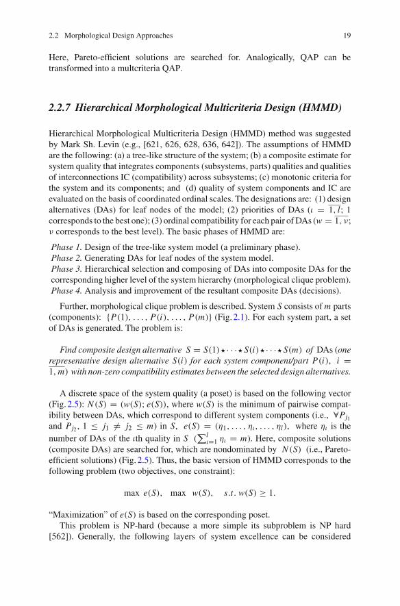
A discrete space of the system quality (a poset) is based on the following vector(Fig. 2.5): N (S) = (w(S); e(S)), where w(S) is the minimum of pairwise compat-ibility between DAs, which correspond to different system components (i.e., ∀Pj1and Pj2 , 1 ≤ j1 �= j2 ≤ m) in S, e(S) = (η1, . . . , ηι, . . . , ηl), where ηι is thenumber of DAs of the ιth quality in S (

∑lι=1 ηι = m). Here, composite solutions

(composite DAs) are searched for, which are nondominated by N (S) (i.e., Pareto-efficient solutions) (Fig. 2.5). Thus, the basic version of HMMD corresponds to thefollowing problem (two objectives, one constraint):

max e(S), max w(S), s.t. w(S) ≥ 1.

“Maximization” of e(S) is based on the corresponding poset.This problem is NP-hard (because a more simple its subproblem is NP hard

[562]). Generally, the following layers of system excellence can be considered


Lattice: w =1

< 3,0,0 >

< 2,1,0 >

< 2,0,1 >

< 1,1,1 >

< 1,0,2 >

< 0,1,2 >

< 0,0,3 >The worstpoint

< 1,2,0 >

< 0,3,0 >

< 0,2,1 >

N(S1)

Lattice: w =2

< 3,0,0 >

< 2,1,0 >

< 2,0,1 >

< 1,1,1 >

< 1,0,2 >

N(S2)

< 0,1,2 >

< 0,0,3 >

< 1,2,0 >

< 0,3,0 >

< 0,2,1 >

Lattice: w =3

The idealpoint< 3,0,0 >

< 2,1,0 >

< 2,0,1 >

< 1,1,1 >

< 1,0,2 >

< 0,1,2 >

< 0,0,3 >

< 1,2,0 >

< 0,3,0 >

< 0,2,1 >

N(S3)

Fig. 2.5 Poset of quality (3 system parts, 3 levels of element quality)

Fig. 2.6 Example ofcomposition

X3(1)

X2(1)

X1(2)

Y2(2)

Y1(3)

Z3(2)

Z2(1)

Z1(1)

X Y Z

S = X Y ZS1 = X2 Y2 Z2

S2 = X1 Y2 Z2

S3 = X1 Y1 Z3

(e.g., [628]): (i) ideal point; (ii) Pareto-efficient points; (iii) a neighborhood ofPareto-efficient DAs (e.g., a composite decision of this set can be transformed into aPareto-efficient point on the basis of an improvement action(s)). Clearly, the com-patibility component of vector N (S) can be considered on the basis of a poset-likescale too (as e(S)). In this case, the discrete space of system excellence will be ananalogical lattice [631, 636].

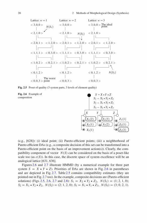
Figures 2.6 and 2.7 illustrate HMMD (by a numerical example for three partsystem S = X � Y � Z ). Priorities of DAs are shown in Fig. 2.6 in parenthesesand are depicted in Fig. 2.7. Table 2.5 contains compatibility estimates (they arepointed out in Fig. 2.7 too). In the example, composite decisions are (Pareto-efficientsolutions) (Figs. 2.5, 2.6, 2.7 and 2.8): S1 = X2 � Y2 � Z2, N (S1) = (1; 2, 1, 0);S2 = X1 � Y2 � Z2, N (S2) = (2; 1, 2, 0); S3 = X1 � Y1 � Z3, N (S3) = (3; 0, 2, 1).

2.3 Design Examples for GSM Network 21

Fig. 2.7 Concentricpresentation

Z3 Z2 Z1 Y2 Y1

X3

X2

X1

2

2

1 3

23

3

3

Table 2.5 Compatibility Y1 Y2 Z1 Z2 Z3

X1 3 2 0 2 3

X2 0 3 0 1 0

X3 0 0 0 0 1

Y1 0 0 3

Y2 0 2 0

Fig. 2.8 Illustration for spaceof quality

N(S1) N(S2)N(S3)

The idealpoint

The worstpoint

w = 1w = 2

w = 3

2.3 Design Examples for GSM Network

In recent two decades, the significance of GSM network has been increased(e.g., [200, 391, 435, 713, 752, 873, 1026]). Thus, there exists a need of the designand maintenance of this kind of communication systems. Here, a numerical examplefor design of GSM network (a modification of an example from [682]) is used toillustrate and to compare several MA-based methods: basic MA, method of closenessto ideal point, Pareto-based MA, multiple choice problem, and HMMD.


GSM network S =A B = (M L) (V U T)

BSS B =V U TSSS A =M L

TRx T :T1,T2,T3,T4,T5

BTS U :U1,U2,U3,U4,U5

BSS V :V1,V2,V3,V4,V5,V6

HLR/AC L:L1,L2,L3,L4

MSC/VLR M:M1,M2,M3,M4,M5

Fig. 2.9 General simplified structure of GSM network

2.3.1 Initial Example

A simplified tree-like model of GSM network is the following (Fig. 2.9):

0. GSM network S = A � B.1. Switching SubSystem SSS (A = M � L).

1.1. Mobile Switching Center/Visitors Location Register MSC/VLR M : M1(Motorola), M2 (Alcatel), M3 (Huawei), M4 (Siemens), and M5 (Ericsson).

1.2. Home Location Register/Authentification Center HLR/AC L : L1 (Motorola),L2 (Ericsson), L3 (Alcatel), and L4 (Huawei).

2. Base Station SubSystem BSS (B = V � U � T ).

2.1. Base Station Controller BSC V : V1 (Motorola), V2 (Ericsson), V3 (Alcatel),V4 (Huawei), V5 (Nokia), and V6 (Siemens).

2.2. Base Transceiver Station BTS U : U1 (Motorola), U2 (Ericsson), U3 (Alca-tel), U4 (Huawei), and U5 (Nokia).

2.3. Transceivers TRx T : T1 (Alcatel), T2 (Ericsson), T3 (Motorola), T4(Huawei), and T5 (Siemens).

Note, an initial set of possible composite decisions contained 3,000 combinations(5 × 4 × 6 × 5 × 5).

The following criteria for system components are considered (weights of criteriaare pointed out in parentheses):

1. M : maximal number of data pathes (1,000 pathes) (Cm1, 0.2); maximal capacityVLR (100,000 subscribers) (Cm2, 0.2); price index (100,000/price (USD)) (Cm3,0.2); power consumption (1/power consumption (kWt)) (Cm4, 0.2); and numberof communication and signaling interfaces (Cm5, 0.2).

2. L: maximal number of subscribers (100,000 subscribers) (Cl1, 0.25); volumeof service provided (Cl2, 0.25); reliability (scale [1, . . . , 10]) (Cl3, 0.25); andintegratability (scale [1, . . . , 10]) (Cl4, 0.25).

3. V : price index (100,000/cost (USD)) (Cv1, 0.25); maximal number of BTS (Cv2,0.25); handover quality (Cv3, 0.25); and throughput (Cv4, 0.25).


Table 2.6 Estimates for M DAs Cm1 Cm2 Cm3 Cm4 Cm5 Priority r

M1 3.7 8.6 6 5.1 4 2

M2 4.0 11 8 7 5 3

M3 4.1 10 9 7 4 3

M4 3.2 7 5 6 3 1

M5 3.5 8.7 6.2 5 4 2

Table 2.7 Estimates for V , L DAs Cv1 Cv2 Cv3 Cv4 Priority r

V1 6 4 3 4 1

V2 7 5 7 7 2

V3 9 7 10 7 3

V4 7 5 8 6 2

V5 6 3 4 4 1

V6 10 6 9 7 3

DAs Cl1 Cl2 Cl3 Cl4 Priority r

L1 9 7 7 8 1

L2 10 4 9 8 1

L3 12 8 10 10 2

L4 9 5 8 8 1

4. U : maximal number of TRx (Cu1, 0.25); capacity (Cu2, 0.25); price index(100,000/cost (USD)) (Cu3, 0.25); and reliability (scale [1, . . . , 10]) (Cu4, 0.25).

5. T : maximum power-carrying capacity (Ct1, 0.3); throughput (Ct2, 0.2); priceindex (100,000/cost(USD)) (Ct3, 0.25); and reliability (scale [1, . . . , 10])(Ct4, 0.25).

Tables 2.6, 2.7 and 2.8, contain estimates of DAs upon criteria above (data from cat-alogues, expert judgment) and their resultant priorities (the priorities are based onmulticriteria ranking by an Electre-like technique [674, 910]). Compatibility esti-mates are contained in Table 2.9 (expert judgment).

2.3.2 Morphological Analysis

In the case of basic MA, binary compatibility estimates are used. To decrease thedimension of the considered numerical example, the following version of MA isexamined. Let us consider more strong requirements to compatibility (Table 2.10):(i) new compatibility estimate equals 1 if the old estimate was equal 3, (ii) newcompatibility estimate equals 1 if the old estimate was equal 0 or 1 or 2. Clearly, herewe can get some negative results, for example: (a) admissible solutions are absent, (b)


Table 2.8 Estimates forU , T

DAs Cu1 Cu2 Cu3 Cu4 Priority r

U1 2 7 5 8 1

U2 4 10 6 10 3

U3 3 9 6 10 2

U4 3 6 3 7 1

U5 3 10 6 9 2

DAs Ct1 Ct2 Ct3 Ct4 Priority r

T1 9 7 10 7 3

T2 6 4 3 4 1

T3 7 5 7 7 2

T4 7 5 8 6 2

T5 6 3 4 4 1

Table 2.9 Compatibility U1 U2 U3 U4 U5 T1 T2 T3 T4 T5

V1 2 2 2 2 3 3 2 2 2 2

V2 3 3 3 2 0 0 3 0 3 2

V3 3 3 3 2 0 0 3 0 3 2

V4 3 2 0 2 3 0 2 0 2 2

V5 3 0 0 2 0 2 2 0 2 2

V6 0 3 2 3 2 3 0 2 2 0

U1 2 0 0 2 3

U2 0 2 0 3 0

U3 0 2 0 3 0

U4 0 3 3 0 0

U5 3 0 2 2 0

L1 L2 L3 L4

M1 3 2 0 3

M2 2 3 2 0

M3 0 2 3 2

M4 2 3 3 3

M5 3 3 0 3

some sufficiently good solutions (e.g., solutions with one/two compatibility estimateat the only admissible/good levels as 1 or 2) will be lost.

As a result, the following admissible DAs can be analyzed:

(1) nine DAs for A: A1 = M1 � L1, A2 = M1 � L4, A3 = M2 � L2, A4 = M3 � L3,A5 = M4 �L2, A6 = M4 �L3, A7 = M5 �L1, A8 = M5 �L2, and A9 = M5 �L4;


Table 2.10 Compatibility U1 U2 U3 U4 U5 T1 T2 T3 T4 T5

V1 0 0 0 0 1 1 0 0 0 0

V2 1 1 1 0 0 0 1 0 1 0

V3 1 1 1 0 0 0 1 0 1 0

V4 1 0 0 0 1 0 0 0 0 0

V5 1 0 0 0 0 0 0 0 0 0

V6 0 1 0 1 0 1 0 0 0 0

U1 0 0 0 0 1

U2 0 0 0 1 0

U3 0 0 0 1 0

U4 0 1 1 0 0

U5 1 0 0 0 0

L1 L2 L3 L4

M1 1 0 0 1

M2 0 1 0 0

M3 0 0 1 0

M4 0 1 1 1

M5 1 1 0 1

(2) five DAs for B: B1 = V1 � U5 � T1, B2 = V2 � U2 � T4, B3 = V2 � U3 � T4,B4 = V3 � U2 � T4, and B5 = V3 � U3 � T4;

and the resultant composite DAs are: S1 = A1 � B1, S2 = A2 � B1, S3 = A3 � B1,S4 = A4�B1, S5 = A5�B1, S6 = A6�B1, S7 = A7�B1, S8 = A8�B1, S9 = A9�B1;S10 = A1 � B2, S11 = A2 � B2, S12 = A3 � B2, S13 = A4 � B2, S14 = A5 � B2,S15 = A6 � B2, S16 = A7 � B2, S17 = A8 � B2, S18 = A9 � B2; S19 = A1 � B3,S20 = A2 � B3, S21 = A3 � B3, S22 = A4 � B3, S23 = A5 � B3, S24 = A6 � B3,S25 = A7 � B3, S26 = A8 � B3, S27 = A9 � B3; S28 = A1 � B4, S29 = A2 � B4,S30 = A3 � B4, S31 = A4 � B4, S32 = A5 � B4, S33 = A6 � B4, S34 = A7 � B4,S35 = A8 � B4, S36 = A9 � B4; S37 = A1 � B5, S38 = A2 � B5, S39 = A3 � B5,S40 = A4 � B5, S41 = A5 � B5, S42 = A6 � B5, S43 = A7 � B5, S44 = A8 � B5, andS45 = A9 � B5.

Finally, the next step has to consist in selection of the best solution.

2.3.3 Method of Closeness to Ideal Point

Here, the initial set of admissible solutions corresponds to the solution set, whichwas obtained in previous case (i.e., basic MA). Evidently, this approach depends onthe kind of the proximity between the ideal point (SI ) and examined solutions.


First of all, let us consider estimate vector for each admissible solution (basicestimates are contained in Tables 2.6, 2.7 and 2.8):

z = (zM

⋃zL

⋃zV

⋃zU

⋃zT )

= (zm1, zm2, zm3, zm4, zm5, zl1, zl2, zl3, zl4, zv1, zv2, zv3, zv4, zu1, zu2, zu3, zu4,

zt1, zt2, zt3, zt4).

On the other hand, it may be reasonable to consider a simplified version of theestimate vector as follows: z = (rM , rL , rV , rU , rT ), where rM , rL , rV , rU , rT arethe priorities of DAs, which are obtained for local DAs (for M , for L , for V , for U ,and for T ; Tables 2.6, 2.7 and 2.8). To simplify the considered example, the secondcase of the estimate vector is used. Thus, the resultant vector estimates (i.e., {z}) forexamined 45 admissible solutions are contained in Table 2.11.

Evidently, it is reasonable to consider the estimate vector for the ideal solution asfollows: z I = (1, 1, 1, 1, 1). Now, let us use a simplified proximity function betweenideal solution I and design alternative as follows (i.e., metric like l2):

ρ(I, D A) =√ ∑

k∈{M,L ,V,U,T }(zk(I ) − zk(D A))2.

Table 2.11 Estimates of admissible solutions

DAs z Proximity to ideal point Membership of Pareto-set

S1 (2, 1, 1, 2, 3) 2.4495 No

S2 (2, 1, 1, 2, 3) 2.4495 No

S3 (3, 1, 1, 2, 3) 3.0 No

S4 (3, 2, 1, 2, 3) 3.1623 No

S5 (1, 1, 1, 2, 3) 2.2361 Yes

S6 (1, 2, 1, 2, 3) 2.4495 No

S7 (2, 1, 1, 2, 3) 2.4495 No

S8 (2, 1, 1, 2, 3) 2.4495 No

S9 (2, 1, 1, 2, 3) 2.4495 No

S10 (2, 1, 2, 3, 2) 2.6458 No

S11 (2, 1, 2, 3, 2) 2.6458 No

S12 (3, 1, 2, 3, 2) 3.1623 No

S13 (3, 2, 2, 3, 2) 3.3166 No

S14 (1, 1, 2, 3, 2) 2.4495 No

S15 (1, 2, 2, 3, 2) 2.6458 No

(continued)


Table 2.11 (continued)

DAs z Proximity to ideal point Membership of Pareto-set

S16 (2, 1, 2, 3, 2) 2.6458 No

S17 (2, 1, 2, 3, 2) 2.6458 No

S18 (2, 1, 2, 3, 2) 2.6458 No

S19 (2, 1, 2, 2, 2) 2.0 No

S20 (2, 1, 2, 2, 2) 2.0 No

S21 (3, 1, 2, 2, 2) 2.6458 No

S22 (3, 2, 2, 2, 2) 2.8284 No

S23 (1, 1, 2, 2, 2) 1.7321 Yes

S24 (1, 2, 2, 2, 2) 2.0 No

S25 (2, 1, 2, 2, 2) 2.0 No

S26 (2, 1, 2, 2, 2) 2.0 No

S27 (2, 1, 2, 2, 2) 2.0 No

S28 (2, 1, 3, 3, 2) 3.1623 No

S29 (2, 1, 3, 3, 2) 3.1623 No

S30 (3, 1, 3, 3, 2) 3.6056 No

S31 (3, 2, 3, 3, 2) 3.7417 No

S32 (1, 1, 3, 3, 2) 3.0 No

S33 (1, 2, 3, 3, 2) 3.1623 No

S34 (2, 1, 3, 3, 2) 3.1623 No

S35 (2, 1, 3, 3, 2) 3.1623 No

S36 (2, 1, 3, 3, 2) 3.1623 No

S37 (2, 1, 3, 2, 2) 2.6458 No

S38 (2, 1, 3, 2, 2) 2.6458 No

S39 (3, 1, 3, 2, 2) 3.1623 No

S40 (3, 2, 3, 2, 2) 3.3166 No

S41 (1, 1, 3, 2, 2) 2.4495 No

S42 (1, 2, 3, 2, 2) 2.6458 No

S43 (2, 1, 3, 2, 2) 2.658 No

S44 (2, 1, 3, 2, 2) 2.6458 No

S45 (2, 1, 3, 2, 2) 2.6458 No

The resultant proximity is presented in Table 2.11. Finally, the best composite DA(by the minimal proximity) is: SI

0 = S23 = A5 � B3 = M3 � L1 � V1 � U2 � T3(ρ = 1.7321). Several composite DAs are very close to the best one, for example:

SI1 = S19 = A1 � B3 = M1 � L1 � V2 � U3 � T4 (ρ = 2.0), SI

2 = S20 = A2 � B3 =M1�L4�V2�U3�T4 (ρ = 2.0), SI

3 = S24 = A6�B3 = M4�L3�V2�U3�T4 (ρ = 2.0),SI

4 = S25 = A7 � B3 = M5 � L1 � V2 � U3 � T4 (ρ = 2.0), SI5 = S26 = A8 � B3 =

M5 � L2 � V3 �U2 � T4 (ρ = 2.0), and SI6 = S27 = A9 � B3 = M5 � L4 � V2 �U3 � T4

(ρ = 2.0).


It may be reasonable to point out several prospective directions for the improve-ment of this method:

(1) consideration of special types of proximity between solutions and the ideal point(e.g., ordinal proximity, vector-like proximity [628], etc.);

(2) usage of special interactive procedures (expert judgment) for the assessment ofthe proximity;

(3) consideration of a set of ideal points (the set can be generated by domainexpert(s)); and

(4) design of special support visualization tools, which will aid domain expert(s)in his/her (their) activity (i.e., generation of the ideal point and assessment ofproximity).

In addition, let us list the basic approaches to generation of the ideal point(s):

1. consideration of design alternative with the estimate vector, in which each com-ponent equals the best value of the design alternatives estimates (by the corre-sponding criterion, i.e., minimum or maximum);

2. consideration of design alternative with the estimate vector, in which each com-ponent equals the best value of the corresponding criterion scale (i.e., minimumor maximum);

3. expert judgment based generation of the best design alternative(s);4. projection of expert judgment based design alternatives into convex shell of the

set of Pareto-efficient points; etc.

2.3.4 Pareto-Based Morphological Analysis

Here, the initial set of admissible solutions corresponds to the previous design case(basic MA). Two approaches can be used for mulricriteria assessment of admissiblesolutions:

1. Basic method: selection of Pareto-efficient solutions over the set of admissiblecomposite solutions on the basis of of usage of the initial set of criteria for assess-ment of each admissible composite DAs;

2. Two-stage method:

(i) assessment of initial components by the corresponding criteria and rankingof the alternative components the get an ordinal priority for each components,

(ii) selection of Pareto-efficient solutions over the set of admissible compositesolutions on the basis of of usage of the vector estimates, which integratepriorities of solution components above. The results of the Pareto-based MAare presented in Table 2.11, i.e., the resultant (Pareto-efficient) DAs are: (i)S P

1 = S5 = A5 � B1 = M4 � L2 �V1 �U5 �T1 and (ii) S P2 = S23 = A5 � B3 =

M4 � L2 � V2 � U3 � T4.


S =M L V U T

M L V U TTRxT1(3)T2(1)T3(2)T4(2)T5(1)

BTSU1(1)U2(3)U3(2)U4(1)U5(2)

BSCV1(1)V2(2)V3(3)V4(2)V5(1)V6(3)

HLR/ACL1(1)L2(1)L3(2)L4(1)

MSC/VLRM1(2)M2(3)M3(3)M4(1)M5(2)

Fig. 2.10 Structure of designed GSM network

It is important to note, the estimate vector for each DA can contain estimates ofcompatibility as well.

2.3.5 Multiple Choice Problem

Multiple choice problem with 5 groups of elements (i.e., for M , L , V , U , T ) is studied(Fig. 2.10, priorities of DAs are shown in parentheses). Here, it is reasonable toexamine multicriteria multiple choice problem. In the example, a simplified problemsolving approach is considered (Table 2.12):

(i) a simple greedy algorithm based on element priorities is used;(ii) for each element (i.e., i, j) ‘profit’ is computed as follows: ci, j = 4 − ri, j ;

(iii) for each element (i.e., i, j) a required resource is computed as follows: ai, j =11−zi, j where zi, j equals: (a) for M : the estimate upon criterion Cm3 (Table 2.6),(b) for L: 1.0, (c) for V : the estimate upon criterion Cv1 (Table 2.7), (d) for U :the estimate upon criterion Cu3 (Table 2.8), and (e) for T : the estimate uponcriterion Cmt3 (Table 2.8).

Thus, the following simplified one-objective problem is considered:

max5∑

i=1

qi∑

j=1

ci j xi j s.t.5∑

i=1

qi∑

j=1

ai j xi j ≤ b,

qi∑

j=1

xi j = 1 ∀i = 1, 5, xi j ∈ {0, 1},

where q1 = 5, q2 = 4, q3 = 6, q4 = 5, q5 = 5. After the usage of the greedyalgorithm, the following composite DAs are obtained (Table 2.12):

(1) resource constraint b = 14: SC1 = M4 � L1 � V6 � U3 � T1,

(2) resource constraint b = 15: SC2 = M4 � L1 � V6 � U1 � T1.


Table 2.12 Example for multiple choice problem

No. DAs Priority Resource ci, j /ai, j Selection Selection

(i, j) r requirement ai, j (constraint: ≤14) (constraint: ≤15)

(1, 1) M1 2 5.0 0.4 No No

(1, 2) M2 3 3.0 0.33 No No

(1, 3) M3 3 2.0 0.5 No No

(1, 4) M4 1 6.0 0.5 Yes Yes

(1, 5) M5 2 4.8 0.38 No No

(2, 1) L1 1 1.0 3.0 Yes Yes

(2, 2) L2 1 1.0 3.0 No No

(2, 3) L3 2 1.0 2.0 No No

(2, 4) L4 1 1.0 3.0 No No

(3, 1) V1 1 5.0 0.6 No No

(3, 2) V2 2 4.0 0.5 No No

(3, 3) V3 3 2.0 0.5 No No

(3, 4) V4 2 4.0 0.5 No No

(3, 5) V5 1 5.0 0.6 No No

(3, 6) V6 3 1.0 1.0 Yes Yes

(4, 1) U1 1 6.0 0.5 No Yes

(4, 2) U2 3 5.0 0.2 No No

(4, 3) U3 2 5.0 0.4 Yes No

(4, 4) U4 3 8.0 0.39 No No

(4, 5) U5 2 5.0 0.4 No No

(5, 1) T1 3 1.0 1.0 Yes Yes

(5, 2) T2 1 8.0 0.39 No No

(5, 3) T3 2 4.0 0.5 No No

(5, 4) T4 2 3.0 0.66 No No

(5, 5) T5 1 7.0 0.42 No No

2.3.6 Hierarchical Morphological Design

A preliminary example for HMMD was presented in [682] (Fig. 2.11, priorities ofDAs are shown in parentheses). For system part A, the following Pareto-efficientcomposite DAs are obtained: (1) A1 = M4 � L2, N (A1) = (3; 2, 0, 0); (2) A2 =M4 � L4, N (A2) = (3; 2, 0, 0). For system part B, the following Pareto-efficientcomposite DAs are obtained: (1) B1 = V5 � U1 � T5, N (B1) = (2; 3, 0, 0); (2)B2 = V5�U4�T2, N (B2) = (2; 3, 0, 0); (3) B3 = V1�U5�T1, N (B3) = (3; 1, 1, 1),and (4) B4 = V2 � U3 � T4, N (B4) = (3; 0, 3, 0). Figure 2.12 illustrates systemquality for B. Now, it is possible to combine the resultant composite DAs as follows(Fig. 2.11):


S =A B = (M L) (V U T)S1 =A1 B1 = (M4 L2) (V5 U1 T5)S2 =A1 B2 = (M4 L2) (V5 U4 T2)S3 =A1 B3 = (M4 L2) (V1 U5 T1)S4 =A2 B1 = (M4 L4) (V5 U1 T5)S5 =A2 B2 = (M4 L4) (V5 U4 T2)S6 =A2 B3 = (M4 L4) (V1 U5 T1)S7 =A1 B4 = (M4 L2) (V2 U3 T4)S8 =A2 B4 = (M4 L4) (V2 U3 T4)

SSS A =M L BSS B =V U TB1 =V5 U1 T5B2 =V5 U4 T2B3 =V1 U5 T1B4 =V2 U3 T4

A1 =M4 L2A2 =M4 L4

M L V U TTRxT1(3)T2(1)T3(2)T4(2)T5(1)

BTSU1(1)U2(3)U3(2)U4(1)U5(2)

BSCV1(1)V2(2)V3(3)V4(2)V5(1)V6(3)

HLR/ACL1(1)L2(1)L3(2)L4(1)

MSC/VLRM1(2)M2(3)M3(3)M4(1)M5(2)

Fig. 2.11 Designed GSM network

(1) SH1 = A1 � B1 = (M4 � L2) � (V5 � U1 � T5);

(2) SH2 = A1 � B2 = (M4 � L2) � (V5 � U4 � T2);

(3) SH3 = A1 � B3 = (M4 � L2) � (V1 � U5 � T1);

(4) SH4 = A2 � B1 = (M4 � L4) � (V5 � U1 � T5);

(5) SH5 = A2 � B2 = (M4 � L4) � (V5 � U4 � T2);

(6) SH6 = A2 � B3 = (M4 � L4) � (V1 � U5 � T1);

(7) SH7 = A1 � B3 = (M4 � L2) � (V2 � U3 � T4); and (8) SH

8 = A2 � B3 =(M4 � L4) � (V2 � U3 � T4).

Finally, it is reasonable to integrate quality vectors for components A and B toobtain the following quality vectors: N (SH

1 ) = (2; 5, 0, 0), N (SH2 ) = (2; 5, 0, 0),

N (SH3 ) = (3; 3, 1, 1), N (SH

4 ) = (2; 5, 0, 0), N (SH5 ) = (3; 3, 1, 1), and N (SH

6 ) =(3; 3, 1, 1). N (SH

7 ) = (3; 2, 3, 0), and N (SH8 ) = (3; 2, 3, 0). Further, the obtained

eight resultant composite decisions can be analyzed to select the best decision (e.g.,additional multicriteria analysis, expert judgment).


N(B1),N(B2)

N(B3) N(B4)

The idealpoint

w =1

w =2

w =3

Fig. 2.12 Space of system quality for B

2.3.7 Comparison of Methods and Discussion

Note, 45 resultant solutions were obtained by basic MA. Table 2.13 integratesresultant composite solutions for four methods: (1) closeness to ideal point method(the best solution and six close solutions), (2) Pareto-based morphological analy-sis (two solutions), (3) multiple choice problem (two solutions), (4) HMMD (eightsolutions).

Now, let us consider a comparison of solution sets above via the following notes:

1. In the case of the first three methods (i.e., MA, closeness to ideal point method, andPareto-based morphological analysis), compatibility estimates in examples areconsidered at levels 0 (incompatible) and 1 (compatible). Generally, this situationcorresponds of a simplified case.

2. In the case of MA, a sufficiently large and rich set of admissible solutions wasobtained: 45. Note, this solution set covers solutions sets for other methods(i.e., closeness to ideal-point method, Pareto-based morphological analysis,HMMD). At the same time, the problem is: to analyze this large solution set.

3. In the case of closeness to ideal point method, only solution SI0 belongs to the set

of Pareto-efficient solutions. Considered solutions {SI1 , SI

2 , SI3 , SI

4 , SI5 , SI

6 }, whichare close to the above-mentioned solution, are not sufficiently good by elements.At the same time, some good solutions are lost, for example: SH

3 , SH5 , SH

6 , SH8 .

4. In the case of Pareto-based morphological analysis, many good solutions are lost,for example: SH

5 , SH6 , SH

8 , etc.5. In the case of multiple choice problem, compatibility estimates are not examined.

As a result, all obtained solutions are inadmissible. It can be reasonable to extendthis kind of optimization models by additional logical constraints, which willformalize the compatibility requirements. But it may lead to complicated models.

6. In the case of HMMD, the set of solutions is sufficiently rich and not very largeat the same time (eight solutions).


Table 2.13 Integration of composite solutions

Method Resultant composite DAs Quality vector (HMMD)

1. Closeness to SI0 = M4 � L2 � V2 � U3 � T4 (3; 2, 3, 0)

ideal point SI1 = M1 � L1 � V2 � U3 � T4 (3; 1, 3, 1)

SI2 = M1 � L4 � V2 � U3 � T4 (3; 1, 4, 0)

SI3 = M4 � L3 � V2 � U3 � T4 (3; 1, 4, 0)

SI4 = M5 � L1 � V2 � U3 � T4 (3; 1, 4, 0)

SI5 = M5 � L2 � V3 � U2 � T4 (3; 1, 2, 2)

SI6 = M5 � L4 � V2 � U3 � T4 (3; 1, 4, 0)

2. Pareto-based S P1 = M4 � L2 � V1 � U5 � T1 (3; 3, 1, 1)

MA S P2 = M4 � L2 � V2 � U3 � T4 (3; 2, 3, 0)

3. Multiple choice SC1 = M4 � L1 � V6 � U3 � T1 (0; 2, 1, 2)

problem SC2 = M4 � L1 � V6 � U1 � T1 (0; 3, 0, 2)

4. HMMD SH1 = M4 � L2 � V5 � U1 � T5 (2; 5, 0, 0)

SH2 = M4 � L2 � V5 � U4 � T2 (2; 5, 0, 0)

SH3 = M4 � L2 � V1 � U5 � T1 (3; 3, 1, 1)

SH4 = M4 � L4 � V5 � U1 � T5 (2; 5, 0, 0)

SH5 = M4 � L4 � V5 � U4 � T2 (3; 3, 1, 0)

SH6 = M4 � L4 � V1 � U5 � T1 (3; 3, 1, 1)

SH7 = M4 � L2 � V2 � U3 � T4 (3; 2, 3, 0)

SH8 = M4 � L4 � V2 � U3 � T4 (3; 2, 3, 0)

Table 2.14 contains an additional qualitative author’s comparison of used meth-ods. Here, computational complexity is depended on enumerative computing andanalysis of all admissible combinatorial solutions (i.e., admissible combinations).In the case of HMMD, the usage of hierarchical system structure decreases com-plexity of the computing process. In the case of Pareto-based MA, an analysis of

Table 2.14 Qualitative comparison of used methods

Method Computationalcomplexity

Taking intoaccountcompatibility

Usefulness forselection of the bestsolutions

Usefulness forexpert(s)

1. MA High Yes, binary Hard Hard

2. Closeness to High Yes, binary Easy Good

Ideal-point(s)

3. Pareto-based MA High Yes, binary Medium, analysis ofpareto-efficientsolutions

Good

4. Multiple choiceProblem

Low/medium None Easy Medium

5. HMMD Low/medium Yes, ordinal Easy Good


Pareto-efficient solutions will required additional enumerative computing. Finally,column “Usefulness for expert(s)” (Table 2.14) corresponds to the following: (i) pos-sibility to include the domain(s) expert(s) or/and decision maker(s) into the solvingprocess (i.e., to include cognitive man-machine procedures into the design frame-work), (ii) understandability of the used design method to domain(s) expert(s) and/ordecision maker(s).

Generally, the selection of the certain kind of morphological methods for adesigned system has to be based on the following: (a) a type of the examined sys-tem class (structure, complexity of component interaction, etc.); (b) structure andcomplexity of the examined representative of the system class; (c) existence of anexperienced design team; (d) possibility to implement some assessment procedures(for assessment of DAs and/or compatibility); (e) possibility to use computationalrecourses (e.g., computing environment, power software, computing personnel), and(f) possibility to use qualified domain(s) experts and/or decision makers.

2.4 Towards Other Approaches

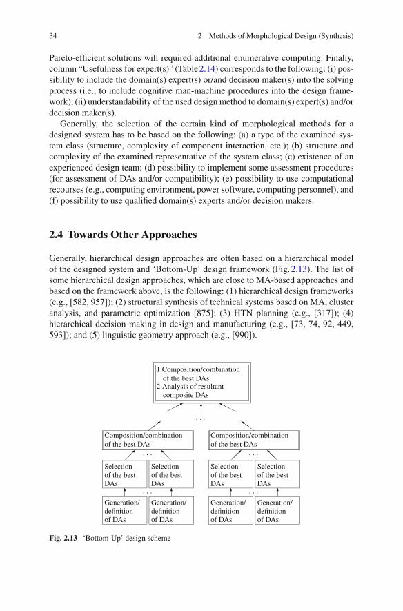
Generally, hierarchical design approaches are often based on a hierarchical modelof the designed system and ‘Bottom-Up’ design framework (Fig. 2.13). The list ofsome hierarchical design approaches, which are close to MA-based approaches andbased on the framework above, is the following: (1) hierarchical design frameworks(e.g., [582, 957]); (2) structural synthesis of technical systems based on MA, clusteranalysis, and parametric optimization [875]; (3) HTN planning (e.g., [317]); (4)hierarchical decision making in design and manufacturing (e.g., [73, 74, 92, 449,593]); and (5) linguistic geometry approach (e.g., [990]).

Generation/definitionof DAs

. . .

. . .

Selectionof the bestDAs



Composition/combinationof the best DAs


. . .

. . .




Composition/combinationof the best DAs

. . .

1.Composition/combinationof the best DAs

2.Analysis of resultantcomposite DAs

Fig. 2.13 ‘Bottom-Up’ design scheme

2.4 Towards Other Approaches 35

Here, it is reasonable to point out some nonlinear programming models, whichare targeted to modular system design as well. First, modular design of series andseries-parallel information processing from the viewpoint of reliable software designwhile taking into account a total budget (i.e., multi-version software design) wasinvestigated in [41, 42, 96]. The authors suggested several generalizations of knap-sack problem with non-linear objective function. Thus, the following kind of theoptimization model for reliable modular software design can be examined (a basiccase) [96]:

maxm∏

i=1

(1 −qi∏

j=1

(1 − pi j xi j ))

s.t.m∑

i=1

qi∑

j=1

di j xi j ≤ b,

qi∑

j=1

xi j ≥ 1 ∀i = 1, m, xi j ∈ {0, 1},

where pi j is a reliability estimate of software module version (i, j) (i.e., version jfor module i), di j is a cost of software module version (i, j). Figure 2.14 illustratesthe design problems above. Evidently, the obtained models are complicated ones andheuristics or enumerative techniques are used for the solving process [41, 42, 96].

In [1104], the problems above are considered regarding the usage of multi-objective genetic algorithms. Second, design problems in chemical engineering sys-tems require often examination of integer and continuous variables at the same timeand, as a result, nonlinear mixed-integer optimization models are formulated andused (e.g., [343, 413]).

Further, it is reasonable to point out constraint-based approaches (e.g., [341, 734,993]) including composite constraint satisfaction problems and AI-based solvingmethods (e.g., [914, 987]).

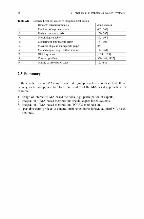
Table 2.15 contains some other research directions, which are close to morpho-logical design (models or/and applications).

......

......

... ......

......

...

(a) (b)

Fig. 2.14 Modular design of series or series-parallel system. a Series scheme. b Series-parallelscheme


Table 2.15 Research directions closed to morphological design

Research directions/models Some sources

1. Problems of representatives [437, 562]

2. Design structure matrix [150, 595]

3. Morphological tables [475, 969]

4. Clustering in multipartite graph [187, 1047]

5. Maximal clique in multipartite graph [254]

6. Method engineering, method service [144, 264]

7. OLAP systems [1024, 1093]

8. Coresets problems [330, 444, 1125]

9. Mining of association rules [10, 984]

2.5 Summary

In the chapter, several MA-based system design approaches were described. It canbe very useful and prospective to extend studies of the MA-based approaches, forexample:

1. design of interactive MA-based methods (e.g., participation of experts),2. integration of MA-based methods and special expert based systems;3. integration of MA-based methods and TOPSIS methods; and4. special research projects as generation of benchmarks for evaluation of MA-based

methods.

http://www.springer.com/978-3-319-09875-3

methods of morphological design (synthesis)

Documents