methods for solving linear least squares...
TRANSCRIPT
stuff
The Least Square Problem (LSQ)Methods for solving Linear LSQComments on the three methods
Regularization techniquesReferences
Methods for solving Linear Least Squares problems
Anibal Sosa
IPM for Linear Programming,September 2009
Anibal SosaMethods for solving Linear Least Squares problems
stuff
The Least Square Problem (LSQ)Methods for solving Linear LSQComments on the three methods
Regularization techniquesReferences
Outline
1 The Least Square Problem (LSQ)Linear Least Square Problems
2 Methods for solving Linear LSQNormal EquationsQR FactorizationSingular Value Decomposition (SVD)
3 Comments on the three methods
4 Regularization techniquesTikhonov regularization and Damped SVDTikhonov regularization order one and two
Anibal SosaMethods for solving Linear Least Squares problems
stuff
The Least Square Problem (LSQ)Methods for solving Linear LSQComments on the three methods
Regularization techniquesReferences
Linear Least Square Problems
The Least Square Problem (LSQ)
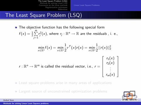
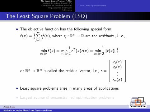
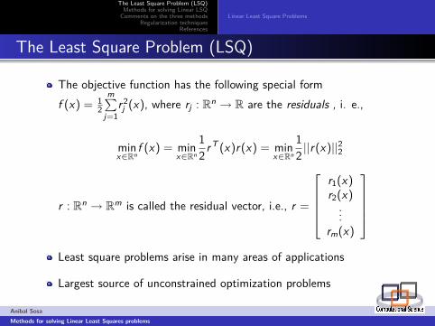
The objective function has the following special formf (x) = 1
2
m∑j=1
r2j (x), where rj : Rn → R are the residuals , i. e.,
minx∈Rn
f (x) = minx∈Rn
12 r
T (x)r(x) = minx∈Rn
12 ||r(x)||22
r : Rn → Rm is called the residual vector, i.e., r =
r1(x)r2(x)...
rm(x)
Least square problems arise in many areas of applications
Largest source of unconstrained optimization problems
Anibal SosaMethods for solving Linear Least Squares problems
stuff
The Least Square Problem (LSQ)Methods for solving Linear LSQComments on the three methods
Regularization techniquesReferences
Linear Least Square Problems
The Least Square Problem (LSQ)
The objective function has the following special formf (x) = 1
2
m∑j=1
r2j (x), where rj : Rn → R are the residuals , i. e.,
minx∈Rn
f (x) = minx∈Rn
12 r
T (x)r(x) = minx∈Rn
12 ||r(x)||22
r : Rn → Rm is called the residual vector, i.e., r =
r1(x)r2(x)...
rm(x)
Least square problems arise in many areas of applications
Largest source of unconstrained optimization problems
Anibal SosaMethods for solving Linear Least Squares problems
stuff
The Least Square Problem (LSQ)Methods for solving Linear LSQComments on the three methods
Regularization techniquesReferences
Linear Least Square Problems
Linear Least Square Problems
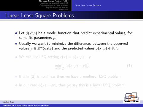
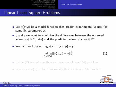
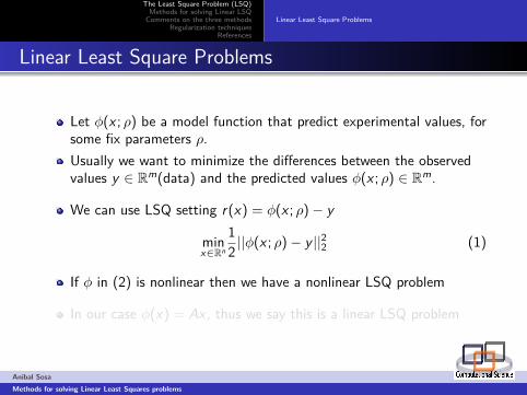
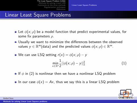
Let φ(x ; ρ) be a model function that predict experimental values, forsome fix parameters ρ.Usually we want to minimize the differences between the observedvalues y ∈ Rm(data) and the predicted values φ(x ; ρ) ∈ Rm.
We can use LSQ setting r(x) = φ(x ; ρ)− y
minx∈Rn
12 ||φ(x ; ρ)− y ||22 (1)
If φ in (2) is nonlinear then we have a nonlinear LSQ problem
In our case φ(x) = Ax , thus we say this is a linear LSQ problem
Anibal SosaMethods for solving Linear Least Squares problems
stuff
The Least Square Problem (LSQ)Methods for solving Linear LSQComments on the three methods
Regularization techniquesReferences
Linear Least Square Problems
Linear Least Square Problems
Let φ(x ; ρ) be a model function that predict experimental values, forsome fix parameters ρ.Usually we want to minimize the differences between the observedvalues y ∈ Rm(data) and the predicted values φ(x ; ρ) ∈ Rm.
We can use LSQ setting r(x) = φ(x ; ρ)− y
minx∈Rn
12 ||φ(x ; ρ)− y ||22 (1)
If φ in (2) is nonlinear then we have a nonlinear LSQ problem
In our case φ(x) = Ax , thus we say this is a linear LSQ problem
Anibal SosaMethods for solving Linear Least Squares problems
stuff
The Least Square Problem (LSQ)Methods for solving Linear LSQComments on the three methods
Regularization techniquesReferences
Linear Least Square Problems
Preliminaries for solving the LSQ problem
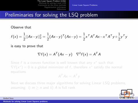
Observe that
f (x) =12 ||Ax−y ||
22 =
12 (Ax−y)T (Ax−y) =
12x
TATAx−xTAT y+12y
T y
is easy to prove that
∇f (x) = AT (Ax − y) ∇2f (x) = ATA
Since f is a convex function is well known that any x∗ such that∇f (x∗) = 0 is a global minimizer of f , therefore x∗ satisfy the normalequations
ATAx = AT y
Next we discuss three major algorithms for solving Linear LSQ problems,assuming: i) m ≥ n and ii) A is full rank
Anibal SosaMethods for solving Linear Least Squares problems
stuff
The Least Square Problem (LSQ)Methods for solving Linear LSQComments on the three methods
Regularization techniquesReferences
Linear Least Square Problems
Preliminaries for solving the LSQ problem
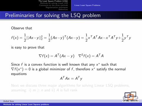
Observe that
f (x) =12 ||Ax−y ||
22 =
12 (Ax−y)T (Ax−y) =
12x
TATAx−xTAT y+12y
T y
is easy to prove that
∇f (x) = AT (Ax − y) ∇2f (x) = ATA
Since f is a convex function is well known that any x∗ such that∇f (x∗) = 0 is a global minimizer of f , therefore x∗ satisfy the normalequations
ATAx = AT y
Next we discuss three major algorithms for solving Linear LSQ problems,assuming: i) m ≥ n and ii) A is full rank
Anibal SosaMethods for solving Linear Least Squares problems
stuff
The Least Square Problem (LSQ)Methods for solving Linear LSQComments on the three methods
Regularization techniquesReferences
Linear Least Square Problems
Preliminaries for solving the LSQ problem
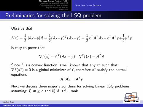
Observe that
f (x) =12 ||Ax−y ||
22 =
12 (Ax−y)T (Ax−y) =
12x
TATAx−xTAT y+12y
T y
is easy to prove that
∇f (x) = AT (Ax − y) ∇2f (x) = ATA
Since f is a convex function is well known that any x∗ such that∇f (x∗) = 0 is a global minimizer of f , therefore x∗ satisfy the normalequations
ATAx = AT y
Next we discuss three major algorithms for solving Linear LSQ problems,assuming: i) m ≥ n and ii) A is full rank
Anibal SosaMethods for solving Linear Least Squares problems

stuff
The Least Square Problem (LSQ)Methods for solving Linear LSQComments on the three methods
Regularization techniquesReferences
Normal EquationsQR FactorizationSingular Value Decomposition (SVD)
Normal Equations
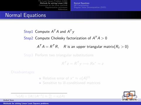
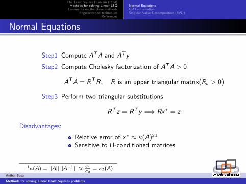
Step1 Compute ATA and AT yStep2 Compute Cholesky factorization of ATA > 0
ATA = RTR, R is an upper triangular matrix(Rii > 0)
Step3 Perform two triangular substitutions
RT z = RT y =⇒ Rx∗ = z
Disadvantages:Relative error of x∗ ≈ κ(A)21
Sensitive to ill-conditioned matrices
1κ(A) = ||A|| ||A−1|| ≈ σ1σn
= κ2(A)Anibal SosaMethods for solving Linear Least Squares problems
stuff
The Least Square Problem (LSQ)Methods for solving Linear LSQComments on the three methods
Regularization techniquesReferences
Normal EquationsQR FactorizationSingular Value Decomposition (SVD)
Normal Equations
Step1 Compute ATA and AT yStep2 Compute Cholesky factorization of ATA > 0
ATA = RTR, R is an upper triangular matrix(Rii > 0)
Step3 Perform two triangular substitutions
RT z = RT y =⇒ Rx∗ = z
Disadvantages:Relative error of x∗ ≈ κ(A)21
Sensitive to ill-conditioned matrices
1κ(A) = ||A|| ||A−1|| ≈ σ1σn
= κ2(A)Anibal SosaMethods for solving Linear Least Squares problems
stuff
The Least Square Problem (LSQ)Methods for solving Linear LSQComments on the three methods
Regularization techniquesReferences
Normal EquationsQR FactorizationSingular Value Decomposition (SVD)
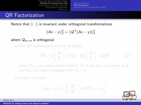
QR FactorizationNotice that || · || is invariant under orthogonal transformations
||Ax − y ||22 = ||QT (Ax − y)||22
where Qm×m is orthogonalThe QR factorization is done as follows
AΠ = Q[
R0
]= [Q1 Q2]
[R0
]= Q1R (2)
where Πn×n is a permutation matrix, Q1 is the first n columns of Qand Rn×n is upper triangular with Rii > 0
Using 2 we have
||Ax − y ||22 =
∣∣∣∣[ QT1
QT2
] (AΠΠT x − y
)∣∣∣∣22
Anibal SosaMethods for solving Linear Least Squares problems
stuff
The Least Square Problem (LSQ)Methods for solving Linear LSQComments on the three methods
Regularization techniquesReferences
Normal EquationsQR FactorizationSingular Value Decomposition (SVD)
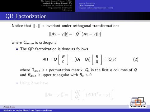
QR FactorizationNotice that || · || is invariant under orthogonal transformations
||Ax − y ||22 = ||QT (Ax − y)||22
where Qm×m is orthogonalThe QR factorization is done as follows
AΠ = Q[
R0
]= [Q1 Q2]
[R0
]= Q1R (2)
where Πn×n is a permutation matrix, Q1 is the first n columns of Qand Rn×n is upper triangular with Rii > 0
Using 2 we have
||Ax − y ||22 =
∣∣∣∣[ QT1
QT2
] (AΠΠT x − y
)∣∣∣∣22
Anibal SosaMethods for solving Linear Least Squares problems
stuff
The Least Square Problem (LSQ)Methods for solving Linear LSQComments on the three methods
Regularization techniquesReferences
Normal EquationsQR FactorizationSingular Value Decomposition (SVD)
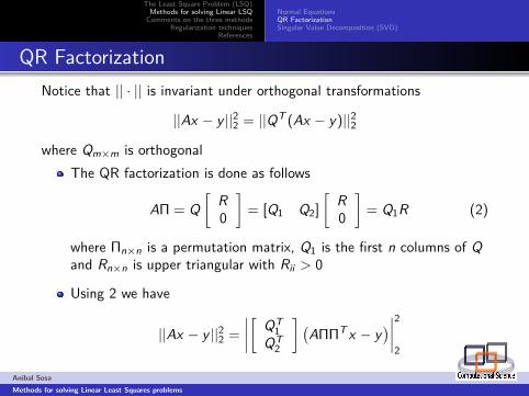
QR FactorizationNotice that || · || is invariant under orthogonal transformations
||Ax − y ||22 = ||QT (Ax − y)||22
where Qm×m is orthogonalThe QR factorization is done as follows
AΠ = Q[
R0
]= [Q1 Q2]
[R0
]= Q1R (2)
where Πn×n is a permutation matrix, Q1 is the first n columns of Qand Rn×n is upper triangular with Rii > 0
Using 2 we have
||Ax − y ||22 =
∣∣∣∣[ QT1
QT2
] (AΠΠT x − y
)∣∣∣∣22
Anibal SosaMethods for solving Linear Least Squares problems
stuff
The Least Square Problem (LSQ)Methods for solving Linear LSQComments on the three methods
Regularization techniquesReferences
Normal EquationsQR FactorizationSingular Value Decomposition (SVD)
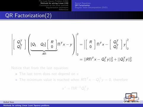
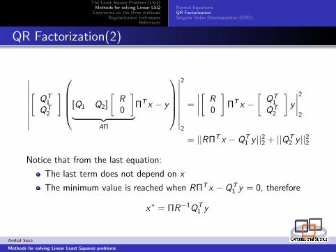
QR Factorization(2)
∣∣∣∣∣∣∣∣∣[
QT1
QT2
][Q1 Q2]
[R0
]︸ ︷︷ ︸
AΠ
ΠT x − y
∣∣∣∣∣∣∣∣∣2
2
=
∣∣∣∣[ R0
]ΠT x −
[QT1
QT2
]y∣∣∣∣22
= ||RΠT x − QT1 y ||22 + ||QT
2 y ||22
Notice that from the last equation:The last term does not depend on xThe minimum value is reached when RΠT x − QT
1 y = 0, therefore
x∗ = ΠR−1QT1 y
Anibal SosaMethods for solving Linear Least Squares problems
stuff
The Least Square Problem (LSQ)Methods for solving Linear LSQComments on the three methods
Regularization techniquesReferences
Normal EquationsQR FactorizationSingular Value Decomposition (SVD)
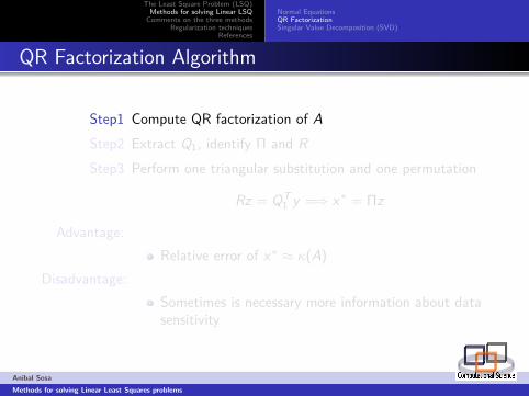
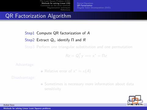
QR Factorization Algorithm
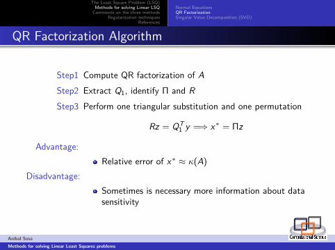
Step1 Compute QR factorization of AStep2 Extract Q1, identify Π and RStep3 Perform one triangular substitution and one permutation
Rz = QT1 y =⇒ x∗ = Πz
Advantage:Relative error of x∗ ≈ κ(A)
Disadvantage:Sometimes is necessary more information about datasensitivity
Anibal SosaMethods for solving Linear Least Squares problems
stuff
The Least Square Problem (LSQ)Methods for solving Linear LSQComments on the three methods
Regularization techniquesReferences
Normal EquationsQR FactorizationSingular Value Decomposition (SVD)
QR Factorization Algorithm
Step1 Compute QR factorization of AStep2 Extract Q1, identify Π and RStep3 Perform one triangular substitution and one permutation
Rz = QT1 y =⇒ x∗ = Πz
Advantage:Relative error of x∗ ≈ κ(A)
Disadvantage:Sometimes is necessary more information about datasensitivity
Anibal SosaMethods for solving Linear Least Squares problems
stuff
The Least Square Problem (LSQ)Methods for solving Linear LSQComments on the three methods
Regularization techniquesReferences
Normal EquationsQR FactorizationSingular Value Decomposition (SVD)
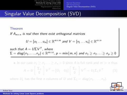
Singular Value Decomposition (SVD)
TheoremIf Am×n is real then there exist orthogonal matrices
U = [u1 . . . um] ∈ Rm×m and V = [v1 . . . vn] ∈ Rn×n
such that A = UΣV T , whereΣ = diag(σ1, . . . , σp) ∈ Rm×n, p = min{m, n} and σ1 ≥ σ2 . . . ≥ σp ≥ 0
In our case σ1 ≥ σ2 . . . ≥ σn > 0 since A is full rank and m� n thus
A = U[
Σ10
]V T = [U1 U2]
[Σ10
]V T = U1Σ1V T (3)
where U1 has the first n columns of U and Σ1 = diag(σ1, . . . , σn).
Anibal SosaMethods for solving Linear Least Squares problems
stuff
The Least Square Problem (LSQ)Methods for solving Linear LSQComments on the three methods
Regularization techniquesReferences
Normal EquationsQR FactorizationSingular Value Decomposition (SVD)
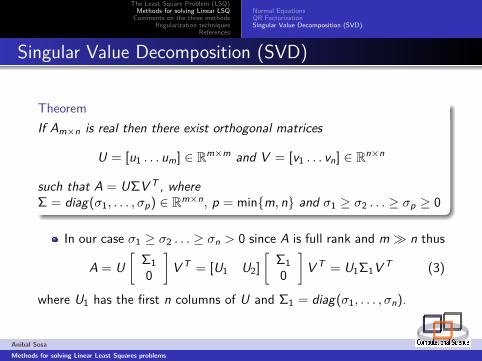
Singular Value Decomposition (SVD)
TheoremIf Am×n is real then there exist orthogonal matrices
U = [u1 . . . um] ∈ Rm×m and V = [v1 . . . vn] ∈ Rn×n
such that A = UΣV T , whereΣ = diag(σ1, . . . , σp) ∈ Rm×n, p = min{m, n} and σ1 ≥ σ2 . . . ≥ σp ≥ 0
In our case σ1 ≥ σ2 . . . ≥ σn > 0 since A is full rank and m� n thus
A = U[
Σ10
]V T = [U1 U2]
[Σ10
]V T = U1Σ1V T (3)
where U1 has the first n columns of U and Σ1 = diag(σ1, . . . , σn).
Anibal SosaMethods for solving Linear Least Squares problems

stuff
The Least Square Problem (LSQ)Methods for solving Linear LSQComments on the three methods
Regularization techniquesReferences
Normal EquationsQR FactorizationSingular Value Decomposition (SVD)
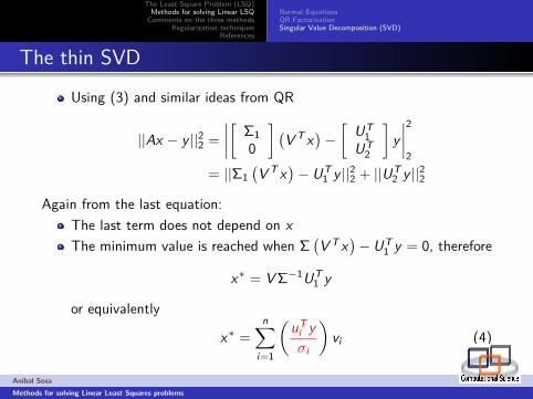
The thin SVD
Using (3) and similar ideas from QR
||Ax − y ||22 =
∣∣∣∣[ Σ10
] (V T x
)−[
UT1
UT2
]y∣∣∣∣22
= ||Σ1(V T x
)− UT
1 y ||22 + ||UT2 y ||22
Again from the last equation:The last term does not depend on xThe minimum value is reached when Σ
(V T x
)−UT
1 y = 0, therefore
x∗ = VΣ−1UT1 y
or equivalently
x∗ =n∑
i=1
(uTi yσi
)vi (4)
Anibal SosaMethods for solving Linear Least Squares problems
stuff
The Least Square Problem (LSQ)Methods for solving Linear LSQComments on the three methods
Regularization techniquesReferences
Normal EquationsQR FactorizationSingular Value Decomposition (SVD)
SVD
Equation (4) gives useful information about x∗ sensitivitySmall changes in A or y can induce large changes in x∗ if σi is smallA is rank defficient when σn
σ1� 1. (σn is the distance from A to the
set of singular matrices)
x∗calculated as in (4) has the smallest 2-norm of all minimizersAdvantage:
Most robust and reliableDisadvantage:
Most expensive
Anibal SosaMethods for solving Linear Least Squares problems
stuff
The Least Square Problem (LSQ)Methods for solving Linear LSQComments on the three methods
Regularization techniquesReferences
Normal Eq. vs QR vs SVD
The Cholesky-based algorithm is practical if m� n ( is easier storeATA), even if A is sparse
The QR algorithm avoid squaring κ(A)
When A is rank-deficient, some σi ≈ 0 thus any vector
x∗ =∑σi 6=0
(uTi yσi
)vi +
∑σi=0
τvi
is also a minimizer of ||Ax − y ||, for τ such that σi ≥ τ,. Thussetting τi = 0 we get the minimum norm solution2
Remark: For very large problems is recommended to use iterativemethods as Conjugate Gradient
2This is a type of filter by doing truncationAnibal SosaMethods for solving Linear Least Squares problems
stuff
The Least Square Problem (LSQ)Methods for solving Linear LSQComments on the three methods
Regularization techniquesReferences
Tikhonov regularization and Damped SVDTikhonov regularization order one and two
Tikhonov regularizationaaRidge regression
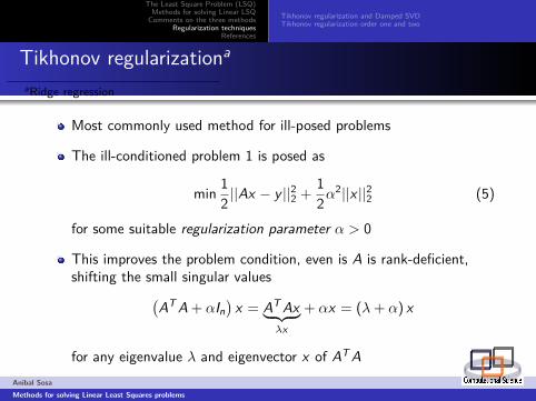
Most commonly used method for ill-posed problems
The ill-conditioned problem 1 is posed as
min 12 ||Ax − y ||22 +
12α
2||x ||22 (5)
for some suitable regularization parameter α > 0
This improves the problem condition, even is A is rank-deficient,shifting the small singular values(
ATA + αIn)x = ATAx︸ ︷︷ ︸
λx
+ αx = (λ+ α) x
for any eigenvalue λ and eigenvector x of ATAAnibal SosaMethods for solving Linear Least Squares problems
stuff
The Least Square Problem (LSQ)Methods for solving Linear LSQComments on the three methods
Regularization techniquesReferences
Tikhonov regularization and Damped SVDTikhonov regularization order one and two
Tikhonov regularizationaaRidge regression
Most commonly used method for ill-posed problems
The ill-conditioned problem 1 is posed as
min 12 ||Ax − y ||22 +
12α
2||x ||22 (5)
for some suitable regularization parameter α > 0
This improves the problem condition, even is A is rank-deficient,shifting the small singular values(
ATA + αIn)x = ATAx︸ ︷︷ ︸
λx
+ αx = (λ+ α) x
for any eigenvalue λ and eigenvector x of ATAAnibal SosaMethods for solving Linear Least Squares problems
stuff
The Least Square Problem (LSQ)Methods for solving Linear LSQComments on the three methods
Regularization techniquesReferences
Tikhonov regularization and Damped SVDTikhonov regularization order one and two
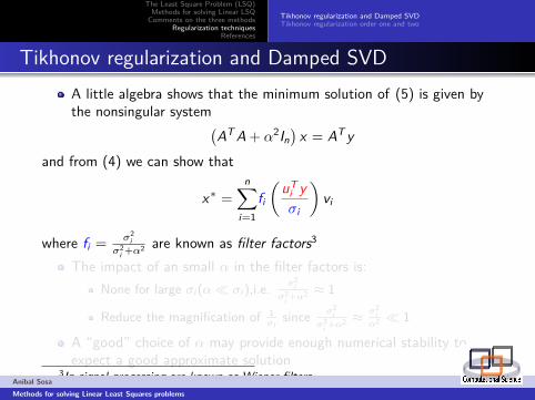
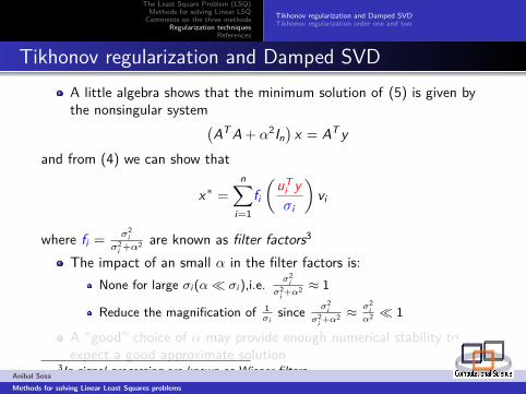
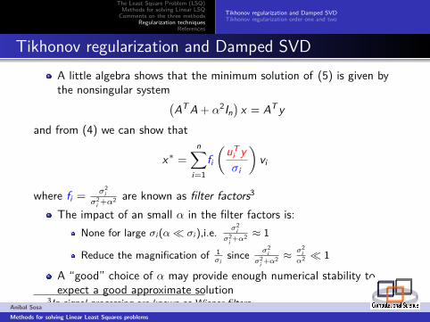
Tikhonov regularization and Damped SVDA little algebra shows that the minimum solution of (5) is given bythe nonsingular system(
ATA + α2In)x = AT y
and from (4) we can show that
x∗ =n∑
i=1fi(uTi yσi
)vi
where fi =σ2iσ2i +α2
are known as filter factors3
The impact of an small α in the filter factors is:None for large σi(α� σi),i.e. σ2i
σ2i +α2≈ 1
Reduce the magnification of 1σi
since σ2iσ2i +α2
≈ σ2iα2� 1
A “good” choice of α may provide enough numerical stability toexpect a good approximate solution
3In signal processing are known as Wiener filtersAnibal SosaMethods for solving Linear Least Squares problems
stuff
The Least Square Problem (LSQ)Methods for solving Linear LSQComments on the three methods
Regularization techniquesReferences
Tikhonov regularization and Damped SVDTikhonov regularization order one and two
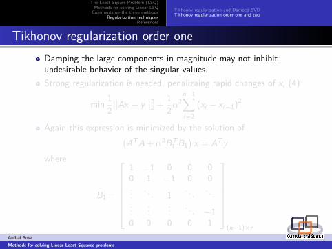
Tikhonov regularization order oneDamping the large components in magnitude may not inhibitundesirable behavior of the singular values.Strong regularization is needed, penalizaing rapid changes of xi (4)
min 12 ||Ax − y ||22 +
12α
2n−1∑i=2
(xi − xi−1)2
Again this expression is minimized by the solution of(ATA + α2BT
1 B1)x = AT y
where
B1 =
1 −1 0 0 00 1 −1 0 0...
. . . 1. . . . . .
......
.... . . −1
0 0 0 0 1
(n−1)×n
Anibal SosaMethods for solving Linear Least Squares problems
stuff
The Least Square Problem (LSQ)Methods for solving Linear LSQComments on the three methods
Regularization techniquesReferences
Tikhonov regularization and Damped SVDTikhonov regularization order one and two
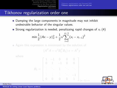
Tikhonov regularization order oneDamping the large components in magnitude may not inhibitundesirable behavior of the singular values.Strong regularization is needed, penalizaing rapid changes of xi (4)
min 12 ||Ax − y ||22 +
12α
2n−1∑i=2
(xi − xi−1)2
Again this expression is minimized by the solution of(ATA + α2BT
1 B1)x = AT y
where
B1 =
1 −1 0 0 00 1 −1 0 0...
. . . 1. . . . . .
......
.... . . −1
0 0 0 0 1
(n−1)×n
Anibal SosaMethods for solving Linear Least Squares problems
stuff
The Least Square Problem (LSQ)Methods for solving Linear LSQComments on the three methods
Regularization techniquesReferences
Tikhonov regularization and Damped SVDTikhonov regularization order one and two
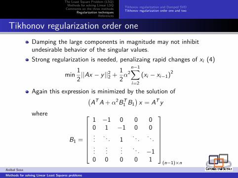
Tikhonov regularization order oneDamping the large components in magnitude may not inhibitundesirable behavior of the singular values.Strong regularization is needed, penalizaing rapid changes of xi (4)
min 12 ||Ax − y ||22 +
12α
2n−1∑i=2
(xi − xi−1)2
Again this expression is minimized by the solution of(ATA + α2BT
1 B1)x = AT y
where
B1 =
1 −1 0 0 00 1 −1 0 0...
. . . 1. . . . . .
......
.... . . −1
0 0 0 0 1
(n−1)×n
Anibal SosaMethods for solving Linear Least Squares problems
stuff
The Least Square Problem (LSQ)Methods for solving Linear LSQComments on the three methods
Regularization techniquesReferences
Tikhonov regularization and Damped SVDTikhonov regularization order one and two
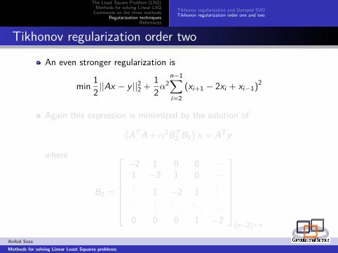
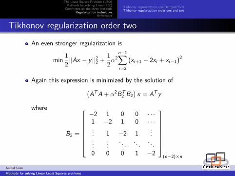
Tikhonov regularization order two
An even stronger regularization is
min 12 ||Ax − y ||22 +
12α
2n−1∑i=2
(xi+1 − 2xi + xi−1)2
Again this expression is minimized by the solution of(ATA + α2BT
2 B2)x = AT y
where
B2 =
−2 1 0 0 · · ·1 −2 1 0 · · ·... 1 −2 1
......
.... . . . . . . . .
0 0 0 1 −2
(n−2)×n
Anibal SosaMethods for solving Linear Least Squares problems
stuff
The Least Square Problem (LSQ)Methods for solving Linear LSQComments on the three methods
Regularization techniquesReferences
Tikhonov regularization and Damped SVDTikhonov regularization order one and two
Tikhonov regularization order two
An even stronger regularization is
min 12 ||Ax − y ||22 +
12α
2n−1∑i=2
(xi+1 − 2xi + xi−1)2
Again this expression is minimized by the solution of(ATA + α2BT
2 B2)x = AT y
where
B2 =
−2 1 0 0 · · ·1 −2 1 0 · · ·... 1 −2 1
......
.... . . . . . . . .
0 0 0 1 −2
(n−2)×n
Anibal SosaMethods for solving Linear Least Squares problems
stuff
The Least Square Problem (LSQ)Methods for solving Linear LSQComments on the three methods
Regularization techniquesReferences
References
Numerical Optimization. J. Nocedal, S. Wright. Second Edition.Springer. 2006
Matrix Computations. G. Golub, Van Loan. Third Edition. JhonsHopkins University Press. 1996
Anibal SosaMethods for solving Linear Least Squares problems