methods for probing new physics at high...
TRANSCRIPT
Methods for Probing New Physics at High Energies
by
Peter B. Denton
Dissertation
Submitted to the Faculty of the
Graduate School of Vanderbilt University
in partial fulfillment of the requirements
for the degree of
DOCTOR OF PHILOSOPHY
in
Physics
August, 2016
Nashville, Tennessee
Approved:
Thomas J. Weiler, Ph.D.
Robert J. Scherrer, Ph.D.
Thomas W. Kephart, Ph.D.
Andreas A. Berlind, Ph.D.
M. Shane Hutson, Ph.D.
Preface
This dissertation covers two broad topics. The title, “Methods for Probing New Physics at HighEnergies,” hopefully encompasses both of them. The first topic is located in part I of this workand is about integral dispersion relations. This is a technique to probe for new physics at energyscales near to the machine energy of a collider. For example, a hadron collider taking data at agiven energy is typically only sensitive to new physics occurring at energy scales about a factor offive to ten beneath the actual machine energy due to parton distribution functions. This techniqueis sensitive to physics happening directly beneath the machine energy in addition to the even moreinteresting case: directly above. Precisely where this technique is sensitive is one of the main topicsof this area of research.
The other topic is located in part II and is about cosmic ray anisotropy at the highest en-ergies. The unanswered questions about cosmic rays at the highest energies are numerous andinterconnected in complicated ways. What may be the first piece of the puzzle to fall into place isdetermining their sources. This work looks to determine if and when the use of spherical harmonicsbecomes sensitive enough to determine these sources.
The completed papers for this work can be found online. For part I on integral dispersionrelations see reference [1] published in Physical Review D. For part II on cosmic ray anisotropy,there are conference proceedings [2] published in the Journal of Physics: Conference Series. Theanalysis of the location of an experiment on anisotropy reconstruction is [3], and the comparisonof different experiments’ abilities to reconstruct anisotropies is [4] published in The AstrophysicalJournal and the Journal of High Energy Astrophysics respectively.
While this dissertation is focused on three papers completed with Tom Weiler at VanderbiltUniversity, other papers were completed at the same time. The first was with Nicusor Arsene,Lauretiu Caramete, and Octavian Micu in Romania on the detectability of quantum black holesin extensive air showers [5]. The next was with Luis Anchordoqui, Haim Goldberg, Thomas Paul,Luiz da Silva, Brian Vlcek, and Tom Weiler on placing limits on Weinberg’s Higgs portal, originallywritten to explain anomalous Neff values, from direct detection and collider experiments [6] whichwas published in Physical Review D. The final was completed at Fermilab with Stephen Parkeand Hisakazu Minakata on a perturbative description of neutrino oscillations in matter [7] whichwas published in the Journal of High Energy Physics, and the code behind this paper is publiclyavailable [8].
ii
Table of Contents
Page
Preface . . . . . . . . . . . . . . . . . . . . . . . . . . . . . . . . . . . . . . . . . . . . . . . . ii
List of Tables . . . . . . . . . . . . . . . . . . . . . . . . . . . . . . . . . . . . . . . . . . . . vi
List of Figures . . . . . . . . . . . . . . . . . . . . . . . . . . . . . . . . . . . . . . . . . . . vii
Part I Integral Dispersion Relations 1
Chapter
1 Introduction and Motivation . . . . . . . . . . . . . . . . . . . . . . . . . . . . . . . . 2
1.1 Introduction . . . . . . . . . . . . . . . . . . . . . . . . . . . . . . . . . . . . . . . . . 21.2 Motivation . . . . . . . . . . . . . . . . . . . . . . . . . . . . . . . . . . . . . . . . . 2
2 Review of Integral Dispersion Relations . . . . . . . . . . . . . . . . . . . . . . . . . 3
2.1 Historical . . . . . . . . . . . . . . . . . . . . . . . . . . . . . . . . . . . . . . . . . . 32.2 Mathematics . . . . . . . . . . . . . . . . . . . . . . . . . . . . . . . . . . . . . . . . 32.3 Scattering Kinematics . . . . . . . . . . . . . . . . . . . . . . . . . . . . . . . . . . . 4
2.3.1 Mandelstam Variables . . . . . . . . . . . . . . . . . . . . . . . . . . . . . . . 42.3.2 Cross Sections . . . . . . . . . . . . . . . . . . . . . . . . . . . . . . . . . . . 5
2.4 Derivation of IDRs . . . . . . . . . . . . . . . . . . . . . . . . . . . . . . . . . . . . . 52.4.1 Froissart Bound . . . . . . . . . . . . . . . . . . . . . . . . . . . . . . . . . . 92.4.2 Pomeranchuk Theorem . . . . . . . . . . . . . . . . . . . . . . . . . . . . . . 9
3 A Simplified Integral Dispersion Relation to Set Expectations . . . . . . . . . . 11
4 Experimental Overview . . . . . . . . . . . . . . . . . . . . . . . . . . . . . . . . . . . 14
4.1 New Physics in the ρ Parameter . . . . . . . . . . . . . . . . . . . . . . . . . . . . . 144.1.1 Approach . . . . . . . . . . . . . . . . . . . . . . . . . . . . . . . . . . . . . . 144.1.2 IDR Independent Calculation of ρ . . . . . . . . . . . . . . . . . . . . . . . . 14
4.2 Forward Scattering Measurements and Fits . . . . . . . . . . . . . . . . . . . . . . . 154.3 The TOTEM Experiment . . . . . . . . . . . . . . . . . . . . . . . . . . . . . . . . . 16
5 Modifying the Cross Section . . . . . . . . . . . . . . . . . . . . . . . . . . . . . . . . 17
5.1 General Modification . . . . . . . . . . . . . . . . . . . . . . . . . . . . . . . . . . . . 175.2 Step Function Modification . . . . . . . . . . . . . . . . . . . . . . . . . . . . . . . . 195.3 A Partonic Model of New Physics . . . . . . . . . . . . . . . . . . . . . . . . . . . . . 19
iii
5.4 A Diffractive Model of New Physics . . . . . . . . . . . . . . . . . . . . . . . . . . . 21
6 Results . . . . . . . . . . . . . . . . . . . . . . . . . . . . . . . . . . . . . . . . . . . . . . 23
6.1 Results From the Step Function Model . . . . . . . . . . . . . . . . . . . . . . . . . . 236.2 Results From the Partonic Model . . . . . . . . . . . . . . . . . . . . . . . . . . . . . 256.3 Results From the Diffractive Model . . . . . . . . . . . . . . . . . . . . . . . . . . . . 26
7 Conclusions . . . . . . . . . . . . . . . . . . . . . . . . . . . . . . . . . . . . . . . . . . . 28
Appendix . . . . . . . . . . . . . . . . . . . . . . . . . . . . . . . . . . . . . . . . . . . . . . 29
A Minimum Transfer Energy in Two Lights to Light + One Heavy Processes . . . . . . 29
Part II Ultra High Energy Cosmic Ray Anisotropy 30
8 Introduction . . . . . . . . . . . . . . . . . . . . . . . . . . . . . . . . . . . . . . . . . . 31
8.1 Introduction . . . . . . . . . . . . . . . . . . . . . . . . . . . . . . . . . . . . . . . . . 318.2 Motivation . . . . . . . . . . . . . . . . . . . . . . . . . . . . . . . . . . . . . . . . . 318.3 Previous Anisotropy Searches . . . . . . . . . . . . . . . . . . . . . . . . . . . . . . . 32
9 Experiments . . . . . . . . . . . . . . . . . . . . . . . . . . . . . . . . . . . . . . . . . . 33
9.1 Current Ground Based Experiments . . . . . . . . . . . . . . . . . . . . . . . . . . . 339.1.1 Pierre Auger Observatory . . . . . . . . . . . . . . . . . . . . . . . . . . . . . 339.1.2 Telescope Array . . . . . . . . . . . . . . . . . . . . . . . . . . . . . . . . . . 339.1.3 Partial Sky Exposure . . . . . . . . . . . . . . . . . . . . . . . . . . . . . . . 34
9.2 Future Space Based Experiments . . . . . . . . . . . . . . . . . . . . . . . . . . . . . 349.3 Event Rates . . . . . . . . . . . . . . . . . . . . . . . . . . . . . . . . . . . . . . . . . 36
10 Tools for Anisotropy Searches . . . . . . . . . . . . . . . . . . . . . . . . . . . . . . . 37
10.1 Spherical harmonics . . . . . . . . . . . . . . . . . . . . . . . . . . . . . . . . . . . . 3710.1.1 Dipole Overview . . . . . . . . . . . . . . . . . . . . . . . . . . . . . . . . . . 3810.1.2 Quadrupole Overview . . . . . . . . . . . . . . . . . . . . . . . . . . . . . . . 38
10.2 Power Spectrum . . . . . . . . . . . . . . . . . . . . . . . . . . . . . . . . . . . . . . 4010.2.1 Nodal Lines . . . . . . . . . . . . . . . . . . . . . . . . . . . . . . . . . . . . . 4010.2.2 Proof of the Rotational Invariance of the Power Spectrum . . . . . . . . . . . 41
10.3 Anisotropy Measure . . . . . . . . . . . . . . . . . . . . . . . . . . . . . . . . . . . . 42
11 Reconstructing Anisotropies . . . . . . . . . . . . . . . . . . . . . . . . . . . . . . . . 44
11.1 Full Sky Coverage . . . . . . . . . . . . . . . . . . . . . . . . . . . . . . . . . . . . . 4411.1.1 Sommers’s Approach for Dipoles . . . . . . . . . . . . . . . . . . . . . . . . . 4411.1.2 Sommers’s Approach for Quadrupoles . . . . . . . . . . . . . . . . . . . . . . 4411.1.3 New Approach for Quadrupoles . . . . . . . . . . . . . . . . . . . . . . . . . . 45
11.2 Partial Sky Coverage . . . . . . . . . . . . . . . . . . . . . . . . . . . . . . . . . . . . 4711.2.1 AP Approach for Dipoles . . . . . . . . . . . . . . . . . . . . . . . . . . . . . 4711.2.2 K-matrix Approach . . . . . . . . . . . . . . . . . . . . . . . . . . . . . . . . 4811.2.3 Comparison of Partial Sky Dipole Approaches . . . . . . . . . . . . . . . . . . 48
12 Reconstructing Quadrupoles at the With Partial Sky Coverage . . . . . . . . . . 50
12.1 Square Brackets . . . . . . . . . . . . . . . . . . . . . . . . . . . . . . . . . . . . . . . 50
iv
12.2 Low Order Multipoles . . . . . . . . . . . . . . . . . . . . . . . . . . . . . . . . . . . 5212.3 Vanishing Quadrupole Component of the Exposure Function . . . . . . . . . . . . . 5212.4 A Simplifying Cutoff . . . . . . . . . . . . . . . . . . . . . . . . . . . . . . . . . . . . 5412.5 Pure Quadrupole . . . . . . . . . . . . . . . . . . . . . . . . . . . . . . . . . . . . . . 5612.6 Numerical Verification for the Pure Quadrupole Case . . . . . . . . . . . . . . . . . . 5612.7 A Quadrupole Purity Test . . . . . . . . . . . . . . . . . . . . . . . . . . . . . . . . . 5712.8 Pure Dipole . . . . . . . . . . . . . . . . . . . . . . . . . . . . . . . . . . . . . . . . . 58
13 Distinguishing Between Dipoles and Quadrupoles . . . . . . . . . . . . . . . . . . 60
14 Results . . . . . . . . . . . . . . . . . . . . . . . . . . . . . . . . . . . . . . . . . . . . . . 62
14.1 Dipole results . . . . . . . . . . . . . . . . . . . . . . . . . . . . . . . . . . . . . . . . 6214.2 Quadrupole results . . . . . . . . . . . . . . . . . . . . . . . . . . . . . . . . . . . . . 62
15 Conclusions . . . . . . . . . . . . . . . . . . . . . . . . . . . . . . . . . . . . . . . . . . . 66
Appendix . . . . . . . . . . . . . . . . . . . . . . . . . . . . . . . . . . . . . . . . . . . . . . 67
B b10-cut . . . . . . . . . . . . . . . . . . . . . . . . . . . . . . . . . . . . . . . . . . . 67C Tables of Low Multipole Square Brackets . . . . . . . . . . . . . . . . . . . . . . . . 68
Bibliography . . . . . . . . . . . . . . . . . . . . . . . . . . . . . . . . . . . . . . . . . . . . 68
v
List of Tables
4.1 Fit parameters to eq. 4.5 from [9] with various analyticity constraints. . . . . . . . . 15
C.1 Values for independent, non-vanishing brackets with ℓ = 0, 1, and 2, when m2 = 0.When m = 0 as well, the brackets are symmetric under interchange of any ℓ values. . 69
C.2 Values for independent, non-vanishing brackets for ℓ = 3 and 4, when m2 = 0. Whenm = 0 as well, the brackets are symmetric under interchange of any ℓ values. . . . . 70
vi
List of Figures
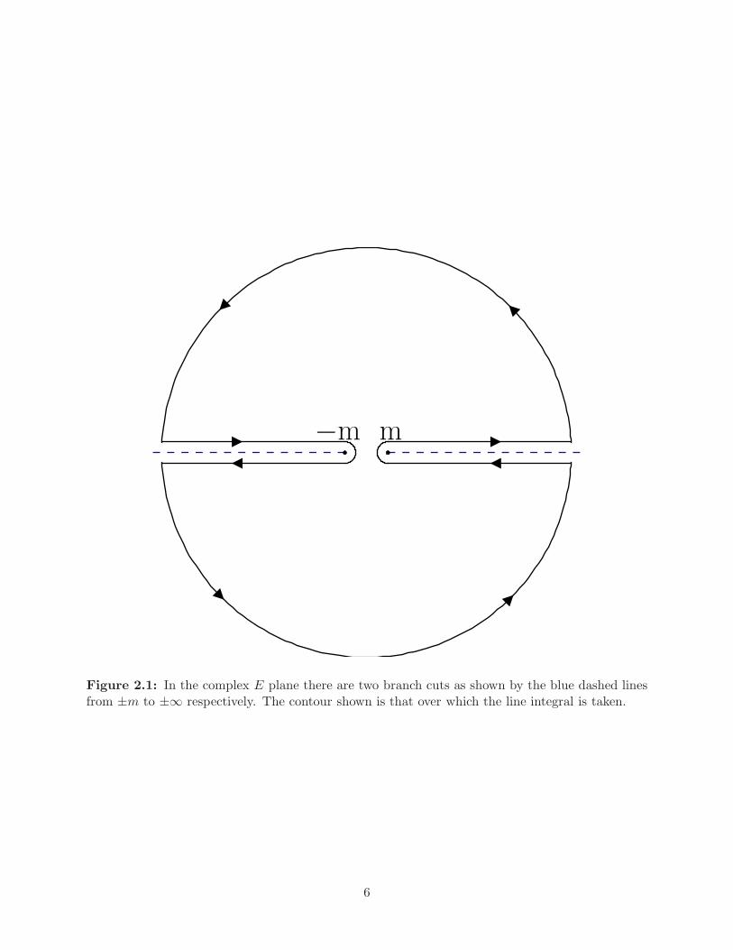
2.1 In the complex E plane there are two branch cuts as shown by the blue dashed linesfrom ±m to ±∞ respectively. The contour shown is that over which the line integralis taken. . . . . . . . . . . . . . . . . . . . . . . . . . . . . . . . . . . . . . . . . . . . 6
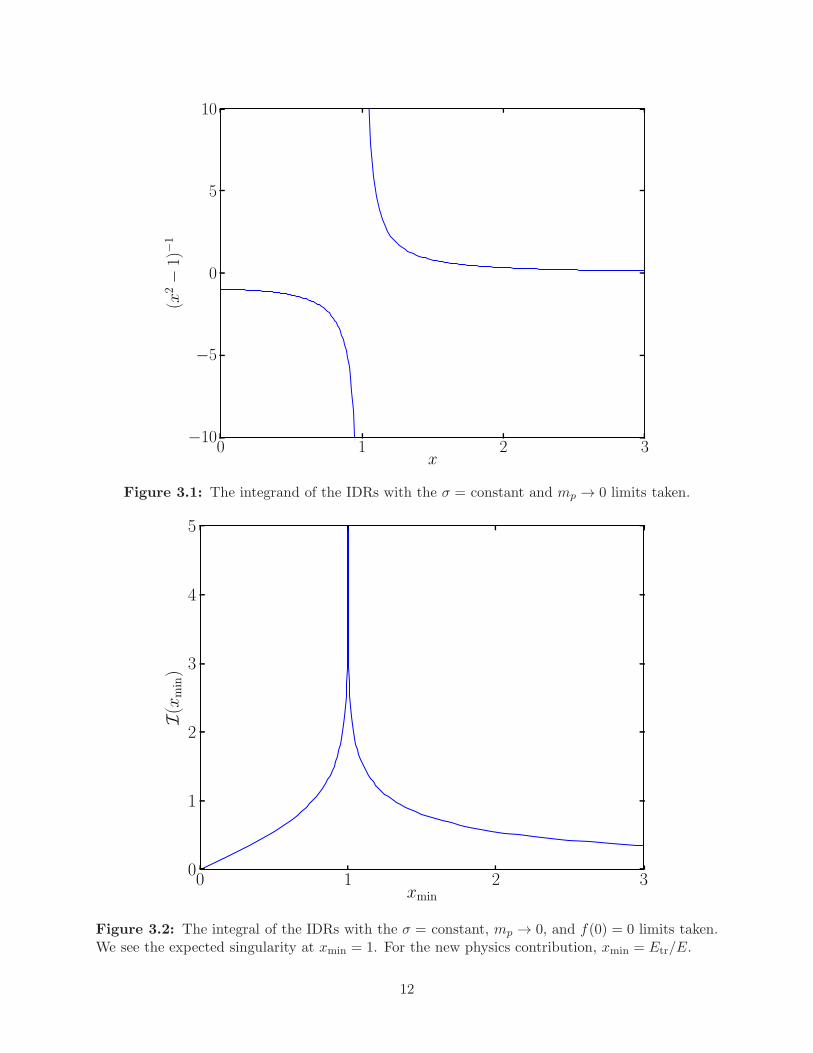
3.1 The integrand of the IDRs with the σ = constant and mp → 0 limits taken. . . . . . 123.2 The integral of the IDRs with the σ = constant, mp → 0, and f(0) = 0 limits taken.
We see the expected singularity at xmin = 1. For the new physics contribution,xmin = Etr/E. . . . . . . . . . . . . . . . . . . . . . . . . . . . . . . . . . . . . . . . . 12
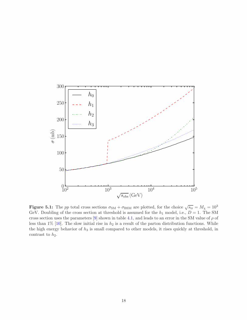
5.1 The pp total cross sections σSM + σBSM are plotted, for the choice√str = Mχ = 103
GeV. Doubling of the cross section at threshold is assumed for the h1 model, i.e.,D = 1. The SM cross section uses the parameters [9] shown in table 4.1, and leadsto an error in the SM value of ρ of less than 1% [10]. The slow initial rise in h2 is aresult of the parton distribution functions. While the high energy behavior of h3 issmall compared to other models, it rises quickly at threshold, in contrast to h2. . . . 18
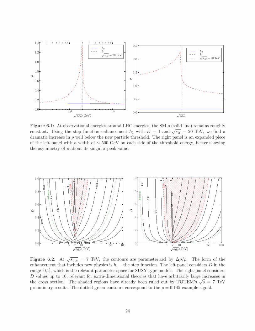
6.1 At observational energies around LHC energies, the SM ρ (solid line) remains roughlyconstant. Using the step function enhancement h1 with D = 1 and
√str = 20 TeV,
we find a dramatic increase in ρ well below the new particle threshold. The rightpanel is an expanded piece of the left panel with a width of ∼ 500 GeV on each sideof the threshold energy, better showing the asymmetry of ρ about its singular peakvalue. . . . . . . . . . . . . . . . . . . . . . . . . . . . . . . . . . . . . . . . . . . . . 24
6.2 At√sobs = 7 TeV, the contours are parameterized by ∆ρ/ρ. The form of the
enhancement that includes new physics is h1 – the step function. The left panelconsiders D in the range [0,1], which is the relevant parameter space for SUSY-typemodels. The right panel considers D values up to 10, relevant for extra-dimensionaltheories that have arbitrarily large increases in the cross section. The shaded regionshave already been ruled out by TOTEM’s
√s = 7 TeV preliminary results. The
dotted green contours correspond to the ρ = 0.145 example signal. . . . . . . . . . . 246.3 The fractional increases in ρ and σ using h2(s) at
√sobs = 7 TeV, versus Mχ. With
the present significance of ρ data, the exclusion region is well above the top of thegraph. The location of the peak is determined by the pdfs. The dotted green linelabeled example presents the value of ∆ρ/ρ corresponding to the ρ = 0.145 examplesignature; from intersecting lines, a new Mχ = 5.1 TeV threshold is predicted. . . . . 25
vii

6.4 The fractional increase in ρ and σ for the h3 model, at√s = 7 TeV. The increase in
ρ compared to its SM value shows a peak of 0.23 at Mχ =√sobs. We also see that
ρ has increased compared to its SM value slightly across a range of energies beyondthe observation energy. With the present significance of ρ data, the exclusion regionis well above the top of the graph. The location of the peak is at threshold sinceh3, like h1, is discontinuous at threshold. The dotted green line presents the valueof ∆ρ/ρ corresponding to the ρ = 0.145 example signature; from intersecting lines,a new Mχ = 9.1 TeV threshold is predicted. . . . . . . . . . . . . . . . . . . . . . . . 27
9.1 Auger’s exposure function normalized to∫
ω(Ω)dΩ = 4π. Note that the exposure isexactly zero for declinations 45 and above. . . . . . . . . . . . . . . . . . . . . . . . 35
9.2 EUSO’s exposure plotted as a function of declination and maximum zenith angle.The vertical axis shows a deviation from uniformity [11]. . . . . . . . . . . . . . . . . 35
10.1 The power spectrum (see eq. 10.8) for nearby galaxies out to z = 0.028 (to d = 120Mpc) based on their positions (left panel), and weighted according to 1/d2 (rightpanel). The 2MRS catalog [12] includes a cut on Milky Way latitudes |b| < 10
which is accounted for in the calculation of the power spectrum, see appendix B. C2
is large because the galaxies roughly form a planar (quadrupolar) structure; C1 inthe right panel is large because we are not in the center of the super cluster, therebyinducing a dipole contribution. (The relative scale between the ordinates of the twofigures carries no information.) . . . . . . . . . . . . . . . . . . . . . . . . . . . . . . 39
10.2 Nodal lines separating excess and deficit regions of sky for various (ℓ,m) pairs. Thetop row shows the (0, 0) monopole, and the partition of the sky into two dipoles,(1, 0) and (1, 1). The middle row shows the quadrupoles (2, 0), (2, 1), and (2, 2). Thebottom row shows the ℓ = 3 partitions, (3, 0), (3, 1), (3, 2), and (3, 3). . . . . . . . . . 40
10.3 Shown are sample sky maps of 500 cosmic rays. The top row corresponds to theαD,true = 1 dipole, while the bottom row corresponds to the αQ,true = 1 quadrupoledistribution. The left and right panels correspond to all sky, space based and partialsky, ground based coverage, respectively. The injected dipole or quadrupole axis isshown as a blue diamond, and the reconstructed direction is shown as a red star.We see that reconstruction of the multipole direction with an event number of 500 isexcellent for an all sky observatory (left panels) and quite good for partial sky Auger(right panels). In practice, αD and αQ are likely much less than unity, and the eventrate for all sky EUSO is expected to be ∼ 9 times that of Auger. Both effects on thecomparison of Auger and EUSO are shown in figs. 14.1 and 14.2. . . . . . . . . . . . 43
11.1 500 directions were simulated with a quadrupolar distribution aligned in a randomdirection, and with Auger’s exposure. Here, αQ is set to unity. The quadrupolestrength was then reconstructed with each of the two techniques. This process wasrepeated 1000 times. Both approaches are correlated - that is when one approachgives a small value of α, the other will as well. . . . . . . . . . . . . . . . . . . . . . . 46
11.2 We simulated 500 cosmic rays with a dipole of amplitude of αD,true = 1 pointing ina random direction, and with the Auger exposure. Then we reconstructed both thedirection and the dipole amplitude 500 times with both reconstruction techniques(AP and K-matrix). In the left panel we show a histogram of the reconstructedvalues of αD,true, and in the right panel the angle (in degrees) between the correctdipole direction and the reconstructed direction. . . . . . . . . . . . . . . . . . . . . 49
viii
12.1 The relative exposure of Auger as a function of declination. Note that the exposureis zero for declinations above 45. The dashed line is the dipole contribution; thecontributions from the higher order multipoles are comparatively small as shown infig. 12.2. . . . . . . . . . . . . . . . . . . . . . . . . . . . . . . . . . . . . . . . . . . . 53
12.2 In the left panel are the coefficients of the experimental exposure, expressed in termsof spherical harmonics at various latitudes, with θm = 60 fixed. In the right panelare the same coefficients in terms of θm, with a0 = −35.2 fixed to the Auger latitude.In the right panel, the solid green ℓ = 2 line lies nearly on top of the c0ℓ = 0 line,which implies not only that c02 is nearly vanishing at the Auger latitude, but alsothat it is independent of θm. . . . . . . . . . . . . . . . . . . . . . . . . . . . . . . . . 53
12.3 Quadrupoles with magnitudes shown on the horizontal axis are injected into anexperiment at the shown latitudes. The error bars for the inferred quadrupolescorrespond to one standard deviation over 500 repetitions with a different symmetryaxis in each repetition. The black line is αQ,rec = αQ,true. The behavior of theinference at a0 = −35.2 away from the line at low values of αQ,true is due to randomfluctuations. The horizontal shift within one value of αQ,true for different latitudesis implemented for clarity only. . . . . . . . . . . . . . . . . . . . . . . . . . . . . . . 57
12.4 Distributions with 500 cosmic rays, Auger’s exposure, maximal quadrupolar aniso-tropy, and varying dipolar anisotropies were simulated. αD was then reconstructedusing the K-matrix approach. Plotted on the vertical axis is the fraction of simula-tions with αD,rec not consistent with zero at a 95% confidence level. . . . . . . . . . 58
13.1 These panels show the results of attempting to reconstruct a dipole (quadrupole)when there is actually a quadrupole (dipole). The top two panels show the effectof attempting to infer a quadrupole moment from a pure dipole state of varyingmagnitudes while the bottom two panels show the effect of attempting to infer thedipole moment from a pure quadrupole state of varying magnitudes. The left twopanels assume Auger’s partial coverage and 250 cosmic rays, while the right panelsassume uniform exposure and the estimated number of events for EUSO (450 mini-mally, and 1000 maximally). The mean values and the one standard deviation errorbars are derived from 500 samplings. Note that the left most data point in each plot(α(D,Q),true = 0) corresponds to the isotropic case, for which the dashed lines are the95% upper limit. Finally, note that the vertical scales vary significantly between thepartial sky low statistics and full sky larger statistics figures. . . . . . . . . . . . . . 61
14.1 Reconstruction of the dipole amplitude and direction across various parameters.Each data point is the mean value (and one standard deviation error bar as appli-cable) determined from 500 independent simulations. The dipole amplitude and di-rection for Auger’s partial coverage were reconstructed with the K-matrix approach.The ordinate on the fourth panel, αtrue
∆αrec, labels the number of standard deviations
above αD = 0. . . . . . . . . . . . . . . . . . . . . . . . . . . . . . . . . . . . . . . . . 6314.2 Reconstruction of the quadrupole amplitude and direction across various parame-
ters. Each data point is the mean value (and one standard deviation error bar asapplicable) determined from 500 independent simulations. The quadrupole ampli-tude and direction for Auger’s partial coverage and the full sky (EUSO) case werereconstructed with Sommers’s approach using the result of chapter 12. The ordinateon the fourth panel, αtrue
∆αrec, labels the number of standard deviations above αQ = 0. . 65
ix
15.1 The red x’s are the analytic calculation of eq. B.13 which line up with the largespikes as expected. On the left is a uniformly generated sky map with a ‘b10-cut’.The data on the right is the unmodified amℓ ’s calculated from the positions of thegalactic data set. . . . . . . . . . . . . . . . . . . . . . . . . . . . . . . . . . . . . . . 68
x

Part I
Integral Dispersion Relations
1
Chapter 1
Introduction and Motivation
1.1 Introduction
This part of the thesis is focused on integral dispersion relations (IDRs). IDRs were widely usedto study the nonperturbative aspects of the strong interaction, but are still a useful tool to relatecore principles such as unitarity and analyticity to physical observables. An article containing thiswork can be found at reference [1]. In the remainder of this chapter we will outline the path ofthis part and motivate using IDRs to probe new physics. In chapter 2 we derive the IDRs fromanalyticity arguments and the optical theorem. A brief history of IDRs is also included. Chapter 3contains a discussion of analytic solutions in simplifying cases as well as some numerical results forcomparison to the nonsimplified, full equations. We also discuss several of the commonly proposedsolutions to this evidence. In chapter 4 we will present the current status of pp, pp total cross sectionmeasurements. We also will discuss the experiments and how they measure the parameter ρ withoutthe use of IDRs. In chapter 5 we turn some of these new physics models into modifications of thetotal pp cross section. In chapter 6 we compile all the results from the various models. Finally, inchapter 7 the conclusions are discussed.
1.2 Motivation
There is a host of evidence that the standard model (SM) of particle physics is not the entirepicture. To this end many experiments have been looking for new physics at various energy scales.
IDRs make use of analyticity to probe energies above (and below) the machine energy at acollider experiment such as the Large Hadron Collider (LHC). Since IDRs relate the scatteringamplitude at one energy to that at every energy up to infinity, they are sensitive to the grossfeatures of the scattering amplitude at all energies, although they are the most sensitive to changesnear the machine energy. Previously strong neutrino interactions at high energy have been discussedin the context of cosmic rays beyond the GZK limit (see part II for more on the GZK limit) [13].This part will focus on hadronic processes only, specifically pp and pp interactions and generalizeddeviations from SM physics. This work describes several possible deviations (chapter 5) from thecanonical cross section (§2.4.1) and how big of an effect they might have.
2

Chapter 2
Review of Integral Dispersion Relations
2.1 Historical
The history of the development of IDRs stretches back nearly 75 years. The initial steps towardstheir derivation started even earlier. In 1926 Kronig [14] and in 1927 Kramers [15] each derivedwhat is known as the Kramers-Kronig relations in the context of measuring the index of refraction.For a given complex valued function χ(ω) = χ1(ω) + iχ2(ω) where χ1,2 ∈ R, they showed,
χ1(ω) =1
πP∫ ∞
−∞
χ2(ω′)
ω′ − ωdω′ ,
χ2(ω) = − 1
πP∫ ∞
−∞
χ1(ω′)
ω′ − ωdω′ ,
(2.1)
where P∫
is the principal value. These relations are known to mathematicians as Hilbert Trans-forms. They contain some of the key mathematical ideas that IDRs exploit. That is, they relatethe real part of χ to an integral over the imaginary part of χ, which is physically related to thetotal cross section by the optical theorem.
The first example of IDRs used with rigor comparable to that used today was in 1954 byM. Gell-Mann, M. L. Goldberg, and W. E. Thirring [16] who helped put IDRs on a sound footing.It was more difficult at the time because the Pomeranchuk theorem lacked the sound experimentalevidence it has since gained at the Tevatron and the LHC (see §2.4.2). The first use of IDRs withpp scattering was in 1964 by P. Soding [17]. Finally, the main reference used in this chapter is from1985 by M. M. Block and R. N. Cahn [18], which covers a broad collection of high energy hadronicscattering topics.
2.2 Mathematics
IDRs are an extension of Cauchy’s integral formula which states that
f(a) =1
2πi
∮
∂A
f(z)
z − adz , (2.2)
where A is a region in C, complex space, and ∂A is its boundary and a ∈ A. We also requirethat f is analytic everywhere in A. Analyticity of a function can be understood simply as beinglocally “sufficiently smooth.” More precisely, a function f(z) is analytic in region A if f is complexdifferentiable everywhere in A. f(z) is complex differentiable on a region if its first derivativecalculated in the usual fashion is continuous and it satisfies the Cauchy-Riemann equations. Wewrite f(z) = u(x, y) + iv(x, y) and z = x + iy with u, v, x, y ∈ R. Then the Cauchy-Riemannequations are,
∂u
∂x=
∂v
∂y,
∂u
∂y= −∂v
∂x.
(2.3)
3
2.3 Scattering Kinematics
The scattering discussion will be presented in two reference frames. The first is the center of mass(momentum) (COM) that is commonly used today. The second is the so called “lab-frame” inwhich one of the particles is considered to be at rest with the necessary boost applied to the otherparticle. Here we will be considering the high energy collisions of particles with equal mass such aspp or pp collisions probed by the Tevatron [19], the Large Hadron Collider (LHC) [20], and extensiveair showers (EAS) measured at experiments like Fly’s Eye (the precursor to the modern TelescopeArray) [21], the Akeno Giant Air Shower Array [22], and the Pierre Auger Observatory [23] throughthe Glauber model [24].
This lab frame approach follows that of Martin M. Block among others and its gained simplicitycan be seen in the symmetry of fig. 2.1 [18]. For an example of what IDRs look like using the centerof mass frame see [25].
Throughout this part we will use the so called “natural units” where ~ = c = 1.
2.3.1 Mandelstam Variables
This discussion of scattering and the derivation of IDRs in section 2.4 generally follow from [18].First, in the COM frame we consider the general 2 → 2 scattering process, where two initial protonsapproaching each other at high energy with 4-momenta p1, p2, elastically scattering (p+p → p+p)to final states with momenta p3, p4. Then the CM energy squared is
s = (p1 + p2)2 = (p3 + p4)
2 = 4(k2 +m2) , (2.4)
where k is the COM momentum, m is the proton mass, and s is the typical Mandelstam variable[26]1.
We can similarly define the transfer energy squared as the next Mandelstam variable t
t = (p1 − p3)2 = (p2 − p4)
2 = −4k2 sin2(
θ
2
)
, (2.5)
where θ is the scattering angle in the COM frame. The final Mandelstam variable is the square ofthe transfer energy plus a switch,
u = (p1 − p4)2 = (p2 − p3)
2 = −4k2 cos2(
θ
2
)
, (2.6)
which gives rise to the useful relation
s+ t+ u = 4m2 . (2.7)
We note that while s ≥ 0, both t, u ≤ 0.In the lab frame,
s = 2(m2 +mE) , (2.8)
where the momentum of the moving particle p and the energy E are related by the usual relationE =
√
p2 +m2. For forward elastic scattering, t = 0, so combining eqs. 2.7 and 2.8 allows us towrite
E =s− u
4m2, (2.9)
which has the nice property that interchanging pp ↔ pp corresponds to the sign change E ↔ −Esince the first interchange is the same as interchanging p2 ↔ −p4. This fact is the justification forworking in the lab frame.
1Interestingly, these commonly used variables were initially introduced in the context of IDRs.
4

2.3.2 Cross Sections
Next we look to relate scattering amplitudes to differential cross sections. Back in the COM framewe have
dσ
dΩCOM= |fCOM|2 , (2.10)
ordσ
dt=
π
k2|fCOM|2 . (2.11)
In the lab frame these formulas look very similar.
dσ
dΩlab= |f |2 , (2.12)
ordσ
dt=
π
p2|f |2 , (2.13)
where for simplicity we define the lab frame scattering amplitude just f .Next we write down the crucial optical theorem in both reference frames.
σtot =4π
kℑfCOM(θ = 0) , (2.14)
and
σtot =4π
pℑf(θL = 0) , (2.15)
where θL is the lab frame scattering angle. Note that θ = 0 ⇒ θL = 0. For several derivations ofthe optical theorem, see [27].
2.4 Derivation of IDRs
We write the scattering amplitude f as the limit of an analytic complex valued function F at t = 0by
fpp,pp(E) = limǫ→0+
F (±E ± iǫ) , (2.16)
using the interchange property of E mentioned after eq. 2.9. That is, the argument of F is acomplex variable.
From the optical theorem, ℑf is related to the cross section which describes physical processes,so ℑF = 0 on, and near, the real axis when there is no physical process at the given energy, and isanalytic there. Everywhere else along the real axis, pp or pp can interact and ℑF flips sign fromabove to below the real axis. This leads to a branch cut2 for |ℜE| > mp as shown by the dashedlines in fig. 2.1.
Since only the imaginary part of F is discontinuous in the imaginary direction and it changessign across the branch cuts while the real part remains the same, we can write
ℑF (E′ + iǫ) = −ℑF (E′ − iǫ) ,
ℜF (E′ + iǫ) = ℜF (E′ − iǫ) ,(2.17)
2There are additional singularities at lower energies where the protons can interact via pion states, but thecontribution to the IDR from these low energy considerations is negligible, as will be shown in chapter 3.
5
m−m
Figure 2.1: In the complex E plane there are two branch cuts as shown by the blue dashed linesfrom ±m to ±∞ respectively. The contour shown is that over which the line integral is taken.
6
F (E′ + iǫ)− F (E′ − iǫ) = 2iℑF (E′ + iǫ) ,
F (E′ + iǫ)− F (E′ − iǫ) = −2iℑF (E′ − iǫ) .(2.18)
We then integrate around a loop where F is analytic. A sketch of this contour is shown infig. 2.1 where the outer curves are taken to the limit |E| → ∞. For the moment we will assumethat the contribution to the integral from the outer curves is zero. From eq. 2.2 we have that
F (E) =1
2πi
[
∫ ∞
mp
dE′F (E′ + iǫ)− F (E′ − iǫ)
E′ − E+
∫ −mp
−∞dE′F (E′ + iǫ)− F (E′ − iǫ)
E′ −E
]
, (2.19)
where the four contributions come from the four straight sections along each side of the two cutsand the small inner curves are negligibly small as ǫ → 0.
Using eq. 2.18, eq. 2.19 becomes
F (E) =1
π
[
∫ ∞
mp
dE′ℑF (E′ + iǫ)
E′ − E+
∫ ∞
mp
dE′ℑF (−E′ − iǫ)
E′ + E
]
. (2.20)
We consider that F may be even or odd in its argument, denoted F+ or F− respectively. Then,
F±(E) =1
π
∫ ∞
mp
dE′ℑF±(E′ + iǫ)
(
1
E′ − E± 1
E′ + E
)
. (2.21)
or
F+(E) =1
π
∫ ∞
mp
dE′ℑF+(E′ + iǫ)
2E′
E′2 − E2,
F−(E) =1
π
∫ ∞
mp
dE′ℑF−(E′ + iǫ)
2E
E′2 − E2.
(2.22)
We write the pp, pp scattering amplitudes in terms of their even and odd (under E ↔ −Einterchange) components,
fpp,pp = f+ ± f− , where f± =1
2(fpp ± fpp) . (2.23)
We define the principal value integral in the traditional sense,
P∫ c
af(x)dx = lim
ǫ→0+
[∫ b−ǫ
af(x)dx+
∫ c
b+ǫf(x)dx
]
, (2.24)
for a < b < c under the conditions that
∫ b
af(x)dx = ±∞ ∀a < b and
∫ c
bf(x)dx = ∓∞ ∀c > b ,
(2.25)
as is the case, for example, for a simple pole, f(x) = g(x)/(x − b) for g(x) continuous. Moregenerally we have that
limǫ→0+
∫ c
a
g(x)
x− b± iǫdx = P
∫ c
a
g(x)
x− bdx∓ iπg(b) , (2.26)
7

the Sokhotski-Plemelj theorem, which makes use of Cauchy’s integral formula, eq. 2.2, for the finalterm. We use the version with the lower signs and substitute x = E′ + iǫ on the LHS to get
limǫ→0+
∫ c
a
g(E′ + iǫ)
E′ − bdE′ = P
∫ c
a
g(x)
x− bdx+ iπg(b) . (2.27)
The LHS is eq. 2.22 after the substitution g → 2E′ℑF+/(E′ + E), 2EℑF−/(E′ + E) and a →
mp, b → E, c → ∞. Then,
F+(E) =1
πP∫ ∞
mp
dE′ℑF+(E′)
2E′
E′2 − E2+ iℑF+(E) ,
F−(E) =1
πP∫ ∞
mp
dE′ℑF−(E′)
2E
E′2 − E2+ iℑF−(E) ,
(2.28)
ℜF+(E) =1
πP∫ ∞
mp
dE′ℑF+(E′)
2E′
E′2 − E2,
ℜF−(E) =1
πP∫ ∞
mp
dE′ℑF−(E′)
2E
E′2 − E2,
(2.29)
which is the simplest version of the IDRs. We pause to note, at this point, the similarity of eqs. 2.1and 2.29.
We now use some forward thinking and admit that we know the shape of ℑF as E′ → ∞. By theoptical theorem (eq. 2.15), ℑf+ ∝ pσtot, and as E′ → ∞, the integrand of the even integral scaleslike σtot which, from the Froissart bound (§2.4.1) and experiments (§4.2), scales like σtot ∝ log2E′.This integral does not converge at infinity, so we must perform a subtraction to gain convergence.In the odd integral we consider a new function G−(E) = F+(E)/E. The odd function from eq. 2.29is,
ℜF+(E) = ℜF+(0) +1
πP∫ ∞
mp
dE′ℑF+(E′)
2E2
E′(E′2 − E2). (2.30)
This new form has several important features. The first is that the integrand is log2 E′/E′2 asE′ → ∞ which goes to zero faster than 1/E′ so the integral converges. The next is that there is anadditional F+(E = 0) term which comes from the pole at E = 0.
On the other hand, ℑf− ∝ p∆σtot, where ∆σtot is the difference between the pp and pp scatteringamplitudes. The Pomeranchuk theorem (§2.4.2) says that ∆σtot → 0 as E′ → ∞ so the resultingintegrand goes to zero faster than 1/E′ and needs no additional subtraction term.
We now take the ǫ → 0 limit and recover the physical amplitude f from the analytic extensionF we have been using. The odd dispersion relation from eq. 2.29 and the singly subtracted IDR,eq. 2.30 are,
ℜf−(E) =1
πP∫ ∞
mp
dE′ℑf−(E′)2E
E′2 − E2,
ℜf+(E) = ℜf+(0) +1
πP∫ ∞
mp
dE′ℑf+(E′)2E2
E′(E′2 − E2).
(2.31)
We can now combine eqs. 2.15, 2.23, 2.31, and the fact that fpp(0) = fpp(0) as described at eq. 2.9
8
to write the useful singly subtracted IDRs:
ℜfpp(E) = ℜfpp(0) +E
4π2P∫ ∞
mp
dE′ p′
E′
[
σpp(E′)
E′ − E− σpp(E
′)E′ + E
]
,
ℜfpp(E) = ℜfpp(0) +E
4π2P∫ ∞
mp
dE′ p′
E′
[
σpp(E′)
E′ − E− σpp(E
′)
E′ + E
]
.
(2.32)
Before continuing, a few features of these integral dispersion relations should be noted. Thefirst is that the scattering amplitude at one energy E (typically referred to as the “machine” energythroughout this part) is dependent on the behavior of the scattering amplitude and thus the crosssection at all energies. It is this fact that we make particular use of in this part. The next is thepole. Both integrals have a pole at E′ = E. So it is at E′ = E where the value of σtot contributesthe most to the integral. Moreover, this pole only occurs for the same process as on the LHS (ppor pp). We also note that the total cross section for the other process is always scaled down sinceE′ + E > E′ − E. Finally there is the addition of a new subtraction term, ℜf(0) which can onlybe determined experimentally.
We also note the existence of doubly subtracted IDRs where the replacement G− = F−/E2 isalso made. These may be necessary in certain cases for convergence, but do not seem to be requiredby experimental data. That is, if the Pomeranchuk theorem isn’t valid (∆σ 6→ 0 as E → ∞) or ifthe total cross section grows like Eα for α ≥ 1 or faster, an additional subtraction (or more) maybe necessary to guarantee convergence.
We define the ratio,
ρpp,pp(E) =ℜfpp,pp(E, t = 0)
ℑfpp,pp(E, t = 0), (2.33)
which allows us to rewrite eq. 2.32 as,
ρpp(E)σpp(E) =4π
pℜfpp(0) +
E
pπP∫ ∞
mp
dE′ p′
E′
[
σpp(E′)
E′ − E− σpp(E
′)E′ + E
]
,
ρpp(E)σpp(E) =4π
pℜfpp(0) +
E
pπP∫ ∞
mp
dE′ p′
E′
[
σpp(E′)
E′ − E− σpp(E
′)E′ + E
]
.
(2.34)
This equation presents the IDRs in the form to be used throughout the remainder of this part.
2.4.1 Froissart Bound
The Froissart bound states that the total hadronic cross section is σ ≤ C log2(E/E0) for somecoefficients C,E0 as E → ∞ [28]. Various proofs of this exist in the literature, and the nature ofthe constants C,E0 have been and still are vigorously debated. Values of C are typically about twoorders of magnitude above those from present experimental reaches [29–31]. This point is importantin that it puts no limits on increasing the cross section so long as it asymptotically (E → ∞) growsno faster than log2E.
2.4.2 Pomeranchuk Theorem
The Pomeranchuk theorem states that at high energies ∆σ ≡ σpp − σpp → 0 [32]. Moreover, thedifference grows no more quickly than log s [33,34]. This fact has been well established by colliderexperiments, where ∆σ ∝∼ s−0.5 [35].
With an understanding of the underlying theory of quantum chromodynamics (QCD), thePomeranchuk theorem can be more simply understood as a statement that at sufficiently high
9

energies baryons are composed of sea quarks and gluons while the valence quarks barely contributeto their composition. As such, p+ p scattering looks identical to p + p scattering for sufficientlyhigh energies.
10
Chapter 3
A Simplified Integral Dispersion Relation to Set Expectations
In this chapter we make three assumptions to reduce the IDRs in eq. 2.34 to a form that canbe integrated analytically to get a feel for the reach and nature of the IDRs. While none of theassumptions are strictly valid, they are useful to reveal the gross features of the dispersion integral.The first assumption is to set mp to zero. Besides replacing the lower limit of integration withzero, this assumption also sets p′/E′ equal to one. The second assumption is to set σpp and σppequal to each other, and to a constant which we call σ0. The final assumption is to set f(0) = 0,a fact that is moderately supported by the data (§4.2). With these assumptions, both dispersionintegrals become
ρσ0 =2σ0π
P∫ ∞
0
dx
x2 − 1, (3.1)
which can then be integrated to
ρ =2
πlog
[ |1− x|1 + x
]∞
0
, (3.2)
where x ≡ E′/E and we note that the integral is singular at x = 1. Blind evaluation of the definiteintegral over the range [0,∞] then gives zero. That this is correct can also be seen in the followingway: by definition of a principal value integral, the definite integral from eq. 3.1 is
limǫ→0
[∫ 1−ǫ
0
dx
x2 − 1+
∫ ∞
1+ǫ
dx
x2 − 1
]
. (3.3)
Replacing x by u ≡ 1x in either integral, maps the integration region into that of the other integral
(for ǫ small), and reveals that the two integrals are equal but with opposite sign. Thus the totalintegral vanishes. In particular, the singularity in the integrand vanishes in the principal value.
In fig. 3.1, we plot the integrand (x2 − 1)−1 of our simplified dispersion integral. As the lowerlimit of integration xmin is moved up from zero, the cancellation above and below the singularityis no longer complete. However, the vanishing of the total integral when integrated from fromzero to infinity allows us replace the integration across the singularity with a simple, manifestlynonsingular integral as follows:
I(xmin) ≡∫ ∞
xmin
dx
x2 − 1=
∫ xmin
0
dx
1− x2. (3.4)
For xmin = 1, the cancellation is maximally incomplete and the integral is infinite. We plot I(xmin)in fig. 3.2. As expected, the integral is everywhere positive, and diverges at xmin = 1. Thedivergence seems unphysical in that it corresponds to either ℑf = 0 ⇒ σtot = 0 by the opticaltheorem which shouldn’t be the case or that ℜf → ∞ ⇒ σtot → ∞ which is also unphysical. Inreality, a step function increase in the integrand is unphysical as the phase space alone requires acontinuous rise in the cross section which then keeps the integral finite.
We may ask how the singularity is approached, from the two cases: above or below. Writingxmin = 1−∆ and 1+∆, we have the two integrals
∫∞1−∆
dxx2−1 and
∫∞1+∆
dxx2−1 . We restrict ourselves
to 0 < ∆ < 1. The first integral crosses the singularity and according to eq. 3.4 is equal to theclearly finite integral
∫ 1−∆0
dx1−x2 . With the replacement x → 1/x, the second integral becomes
∫
11+∆
0dx
1−x2 . Thus, the two integrations differ only in the upper limit of integration. At first order
11
0 1 2 3x
−10
−5
0
5
10
(x2−1)
−1
Figure 3.1: The integrand of the IDRs with the σ = constant and mp → 0 limits taken.
0 1 2 3xmin
0
1
2
3
4
5
I(xmin)
Figure 3.2: The integral of the IDRs with the σ = constant, mp → 0, and f(0) = 0 limits taken.We see the expected singularity at xmin = 1. For the new physics contribution, xmin = Etr/E.
12
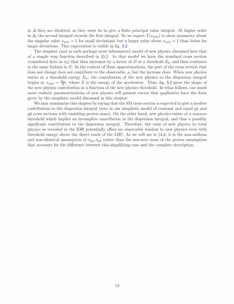
in ∆ they are identical, as they must be to give a finite principal value integral. At higher orderin ∆, the second integral exceeds the first integral. So we expect I(xmin) to show symmetry aboutthe singular value xmin = 1 for small deviations, but a larger value above xmin = 1 than below forlarger deviations. This expectation is visible in fig. 3.2.
The simplest (and as such perhaps most informative) model of new physics discussed here thatof a simple step function described in §5.2. In that model we have the standard cross section(considered here as σ0) that then increases by a factor of D at a threshold Etr and then continuesin the same fashion in E. In the context of these approximations, the part of the cross section thatdoes not change does not contribute to the observable, ρ, but the increase does. When new physicsenters at a threshold energy Etr, the contribution of the new physics to the dispersion integralbegins at xmin = Etr
E , where E is the energy of the accelerator. Thus, fig. 3.2 gives the shape ofthe new physics contribution as a function of the new physics threshold. In what follows, our muchmore realistic parametrizations of new physics will present curves that qualitative have the formgiven by the simplistic model discussed in this chapter.
We may summarize this chapter by saying that the SM cross section is expected to give a modestcontribution to the dispersion integral (zero in our simplistic model of constant and equal pp andpp cross sections with vanishing proton mass). On the other hand, new physics enters at a nonzerothreshold which implies an incomplete cancellation in the dispersion integral, and thus a possiblysignificant contribution to the dispersion integral. Therefore, the ratio of new physics to totalphysics as revealed in the IDR potentially offers an observable window to new physics even withthreshold energy above the direct reach of the LHC. As we will see in §4.2, it is the non-uniformand non-identical assumption of σpp, σpp rather than the non-zero mass of the proton assumptionthat accounts for the difference between this simplifying case and the complete description.
13
Chapter 4
Experimental Overview
4.1 New Physics in the ρ Parameter
4.1.1 Approach
While eq. 2.34 and the other versions of the IDRs relate the total cross section, σtot, at one energyto that at all other energies, this alone does not allow for the discovery of new physics. If the crosssection has a measurable change at the machine’s energy from IDRs due to new physics at higherenergy scales, the presence of new physics can already be inferred via direct production of the newstates without the additional use of IDRs. On the other hand, if the new physics cannot yet beproduced directly, IDRs can infer the presence of new physics near the machine energy without anychange in the cross section. A separate measurement must be made that makes proper use of thepower of IDRs, and that is where the ρ parameter, defined in eq. 2.33, comes in.
The general strategy that we will use to explore new physics is to first use the IDR to calculateρ at a particular energy (an LHC energy) without the inclusion of new physics by assuming that thecross section continues to rise in the expected fashion. Then we calculate ρ at the same energy withthe inclusion of the new physics cross section. Since ρ can be calculated at experiments withoutIDRs in a model-independent fashion, as described in §4.1.2, enhancements of the cross section canbe either identified or ruled out by comparing theoretical and experimental values of ρ(E).
4.1.2 IDR Independent Calculation of ρ
To extract a value for ρ in an IDR independent fashion, one invokes the optical theorem andextrapolates dσ/dt to t = 0, as shown below. The cross section is related to the scattering amplitudeby a simple exponential at low |t|. Recall from eq. 2.11 that the differential cross section in theCOM is
dσ
dt=
π
k2|f |2 . (4.1)
At t = 0 one has
dσ
dt
∣
∣
∣
∣
t=0
=π
k2|ℜf(t = 0) + iℑf(t = 0)|2
=π
k2|(ρ+ i)ℑf(t = 0)|2 .
(4.2)
Making use of the optical theorem, σtot = (4π/k)ℑf(t = 0), one arrives at
16πdσ
dt
∣
∣
∣
∣
t=0
= (ρ2 + 1)σ2tot . (4.3)
From [18], the pp differential cross section in the low t limit is well approximated by
dσ
dt∝ eBt , (4.4)
where B is the “slope parameter,” assumed and measured to be very nearly constant. Thus, ameasurement or estimate of σtot and an extrapolation of dσ/dt to t = 0 via the measured slope
14
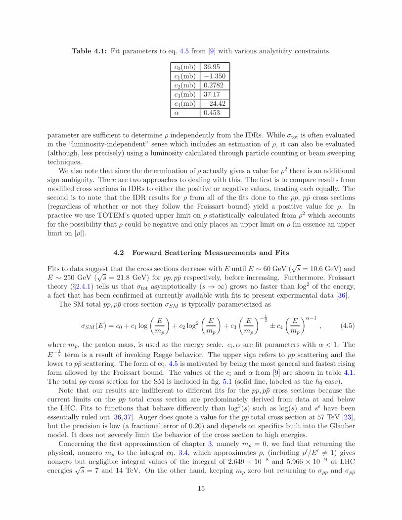
Table 4.1: Fit parameters to eq. 4.5 from [9] with various analyticity constraints.
c0(mb) 36.95
c1(mb) −1.350
c2(mb) 0.2782
c3(mb) 37.17
c4(mb) −24.42
α 0.453
parameter are sufficient to determine ρ independently from the IDRs. While σtot is often evaluatedin the “luminosity-independent” sense which includes an estimation of ρ, it can also be evaluated(although, less precisely) using a luminosity calculated through particle counting or beam sweepingtechniques.
We also note that since the determination of ρ actually gives a value for ρ2 there is an additionalsign ambiguity. There are two approaches to dealing with this. The first is to compare results frommodified cross sections in IDRs to either the positive or negative values, treating each equally. Thesecond is to note that the IDR results for ρ from all of the fits done to the pp, pp cross sections(regardless of whether or not they follow the Froissart bound) yield a positive value for ρ. Inpractice we use TOTEM’s quoted upper limit on ρ statistically calculated from ρ2 which accountsfor the possibility that ρ could be negative and only places an upper limit on ρ (in essence an upperlimit on |ρ|).
4.2 Forward Scattering Measurements and Fits
Fits to data suggest that the cross sections decrease with E until E ∼ 60 GeV (√s = 10.6 GeV) and
E ∼ 250 GeV (√s = 21.8 GeV) for pp, pp respectively, before increasing. Furthermore, Froissart
theory (§2.4.1) tells us that σtot asymptotically (s → ∞) grows no faster than log2 of the energy,a fact that has been confirmed at currently available with fits to present experimental data [36].
The SM total pp, pp cross section σSM is typically parameterized as
σSM (E) = c0 + c1 log
(
E
mp
)
+ c2 log2
(
E
mp
)
+ c3
(
E
mp
)− 12
± c4
(
E
mp
)α−1
, (4.5)
where mp, the proton mass, is used as the energy scale. ci, α are fit parameters with α < 1. The
E− 12 term is a result of invoking Regge behavior. The upper sign refers to pp scattering and the
lower to pp scattering. The form of eq. 4.5 is motivated by being the most general and fastest risingform allowed by the Froissart bound. The values of the ci and α from [9] are shown in table 4.1.The total pp cross section for the SM is included in fig. 5.1 (solid line, labeled as the h0 case).
Note that our results are indifferent to different fits for the pp, pp cross sections because thecurrent limits on the pp total cross section are predominately derived from data at and belowthe LHC. Fits to functions that behave differently than log2(s) such as log(s) and sǫ have beenessentially ruled out [36,37]. Auger does quote a value for the pp total cross section at 57 TeV [23],but the precision is low (a fractional error of 0.20) and depends on specifics built into the Glaubermodel. It does not severely limit the behavior of the cross section to high energies.
Concerning the first approximation of chapter 3, namely mp = 0, we find that returning thephysical, nonzero mp to the integral eq. 3.4, which approximates ρ, (including p′/E′ 6= 1) givesnonzero but negligible integral values of the integral of 2.649 × 10⁻⁸ and 5.966 × 10⁻⁹ at LHCenergies
√s = 7 and 14 TeV. On the other hand, keeping mp zero but returning to σpp and σpp
15
their realistic energy dependences yields nonzero integral values of 0.1345 and 0.1309 at√s = 7
and 14 TeV. And finally, using nonzero mp and realistic pp and pp cross sections returns the values0.1345 and 0.1309 at
√s = 7 and 14 TeV. The final two integration sets (realistic σ’s and zero
or nonzero mp) agree to about seven to eight decimal places respectively (on the order of m2p/s).
The conclusion is that the mp → 0 approximation is generally a valid one, whereas the constantand equal SM cross section approximation in the previous section is not. However, the integralcontributions of the SM to the IDRs (the solid lines in fig. 6.1) are not large, and we are encouragedto pursue further the contributions that might arise due to physics beyond the SM.
For the subtraction constant, we will take f(0) = 0, since the value from the fits above isf(0) = −0.073 ± 0.67 mb GeV. We note that even at the value 1σ away from zero, the term4π f(0)/(p σpp) at LHC energies contributes less than one part in 105 to ρ.
4.3 The TOTEM Experiment
The TOTal Elastic and diffractive cross section Measurement (TOTEM) experiment at the LHCis designed to measure forward cross sections by probing very low |t| regions [38]. TOTEM placesa series of Roman pot detectors very close to the beam and very far from the interaction point.With improved LHC optics, TOTEM should be able to provide an improved measurement of ρindependent of IDRs [39]. A comparison of TOTEM’s ρ, so determined, with the IDR predictionof ρ, then provides the potential evidence for new physics.
Similarly, the Absolute Luminosity For ATLAS (ALFA) [40] experiment, the LHC forward(LHCf [41] experiment, along with a host of others will also make comparable measurements in anattempt to improve the precision of the luminosity calculation, which is necessary to infer σtot, andthen to infer ρ without the use of IDRs [42] (see §4.1). Thus, there are several experiments thataim to measure the total cross section. These offer hope for smaller error bars on IDR independentdeterminations of the crucial parameter ρ(E).
A√s = 7 TeV, the TOTEM article presented a state of the art value for the IDR independent ρ,
of ρ = 0.145 with error bars of ∼ 60% [20]. TOTEM cited a 95% significance level (roughly speaking,a 2σ bound) that ρ < 0.32. Comparing this to the SM prediction of ρ(
√s = 7 TeV) = 0.1345 gives
an upper limit of the fractional increase (ρ − ρSM)/ρSM = 1.38 at the 95% significance level. Forbrevity, in what follows we denote (ρ − ρSM)/ρSM as ∆ρ/ρ. In addition, an early report fromTOTEM gives their error estimate as ∼ 0.04 from their
√s = 8 TeV analysis [43] corresponding to
a fractional error of 30%, thus cutting the error in half.As an illustrative example of what a future determination of ρmight mean for the IDR technique,
we investigate a definite value for ρ; we choose as the definite value the experimentally inferredmean value ρ(
√s = 7 TeV) = 0.145. For this example, the fractional increase in ρ is ∆ρ/ρ = 7.8%.
This value for ρ is chosen for illustration only, as it offers insight into the merit of IDRs shouldexperiments greatly reduce their errors in the inference of ρ.
Compared to the presently published TOTEM error of 63%, the “new physics increase” hasnegligible significance, ∼ 0.1σ. With the ongoing analysis at TOTEM, the new significance isexpected to be ∼ 0.25σ [43]. Clearly, further improvement in the inference of ρ is needed for theprogram constructed in this part. Another reduction in error by about a factor of four (eight) wouldgive a 1(2)σ significance to our illustrative example. One must hope that either the measured erroris reduced significantly in the next LHC run, the new physics contribution to the cross section islarger than our chosen example, or both.
16
Chapter 5
Modifying the Cross Section
5.1 General Modification
We consider a class of modifications to the total pp cross section of the form
σ(s) = σSM(s)[1 + hi(s)] , (5.1)
where σSM is the SM cross section. That is, it is the cross section that has been observed so farconsistent with SM physics. σ is the true cross section. In general, the hi will be zero up to somethreshold str and 0 ≤ lims→∞ hi(s) < ∞. We apply the same enhancement to both σpp and σppsince, by the Pomeranchuk theorem discussed in §2.4.2, each cross section should respond to newphysics in the same way at energies well above the proton mass.
We use this form as it allows for modifications to turn on at an arbitrary energy, preserving themeasured fit, but also retaining the asymptotic limit predicted by the Froissart bound in §2.4.1.This form guarantees that σ will continue to grow at the same rate at σSM.
The first model we will present in §5.2 is a simple step function at str. This model results in anespecially close analogy to the idealized IDRs we discussed in chapter 3. In particular, this modelyields a singularity in the IDR integrand at E = Etr and therefore a singular value for ρ(E = Etr).
More realistically, we expect phase space to present a cross section for new physics that has nojump discontinuity at threshold. For example, two body phase space is β/8π, where β is eitherparticle velocity in the COM frame; at threshold, β is identically zero. Furthermore, includingparton distribution functions to the model also yields a zero cross section at threshold. The newphysics matrix elements may also vanish right at threshold. So we are led to the next two modelsof BSM physics. The second model we present in §5.3 involves hard-scattering parton productionof new particles, while the third model in §5.4 is constructed from diffractive phenomenology. Thesecond and third models provide cross section modifications that vanish at threshold, leading tofinite values for ρ(E = Etr).
Since only the first model, the step function, yields a nonzero change in the cross sectionat threshold, the ρ-value resulting from model h1 should be considered an upper bound to thecontribution of new physics BSM. The bounding of cross sections by the h1 step function model isevident in fig. 5.1, where we show the SM cross section (given by zero enhancement and labeled byh0 = 0) and its enhancements (hi, i = 1, 2, 3) by the three new physics models that are presentedin detail below.
No new conserved quantum number is assumed in our models (valid, e.g., for broken R-paritySUSY models). Thus, energy is the only impediment to production of heavy new single particles,and the heavy single mass value Mχ determines Etr. Without a new quantum number, the newparticle would decay to SM particles, and due to its large mass, decay very quickly. Consequently,other than invariant mass combinatorics, there is no good signature of the new particle’s production.One may have to rely on IDRs and/or an anomalous ∆σ for new particle identification. Thus, weplot ∆ρ/ρ and ∆σ/σ versus Mχ (Mχ =
√str − 2mp ≈ √
str), to see if the IDR technique canidentify new physics via an anomalous ρ measurement, before the new physics would be directlynoticeable in the cross section increase at the next high energy collider.
17
102 103 104 105√sobs (GeV)
0
50
100
150
200
250
300
σ(m
b)
h0
h1
h2
h3
Figure 5.1: The pp total cross sections σSM + σBSM are plotted, for the choice√str = Mχ = 103
GeV. Doubling of the cross section at threshold is assumed for the h1 model, i.e., D = 1. The SMcross section uses the parameters [9] shown in table 4.1, and leads to an error in the SM value of ρ ofless than 1% [10]. The slow initial rise in h2 is a result of the parton distribution functions. Whilethe high energy behavior of h3 is small compared to other models, it rises quickly at threshold, incontrast to h2.
18

5.2 Step Function Modification
A simple example function for BSM physics is
h1(s) = DΘ(s− str) , (5.2)
a step-wise jump in cross section at the threshold COM energy√str. The parameter D is a measure
of the size of the new cross section relative to the SM. For example, in the event that new physicsexactly doubles the cross section at s = str, then D = 1. Modifying σSM in the form of eq. 5.2guarantees that the new total cross section σ continues to grow as fast as σSM ∝ log2 s (but notfaster), and that the new physics contribution remains large over a sizable energy range beyondthe threshold energy.
As mentioned above, an unphysical aspect of the step function enhancement is a non-vanishingcross section at threshold, which leads to the uncanceled singularity in the IDR integrand at E = Etr
and a singular value for ρ(E = Etr) as shown in figs. 3.1 and 3.2. However, the model has redeemablevalue in that the width of the singularity is small since it is valid away from the singularity. Thus,the model offers a meaningful upper bound to new particle production away from the singularity.
5.3 A Partonic Model of New Physics
The most popular model of new physics at the electroweak symmetry breaking scale is R-paritypreserving supersymmetry (SUSY), with masses tuned to the EW scale to stabilize the ratiomh/MPlanck (the “hierarchy problem”). Unfortunately, R-parity conservation requires s, t, andu to have EW-scale values, which severely suppresses the SUSY cross section to ∼ 10−10 timesthe SM cross section. However, as LHC limits on R-parity conserving SUSY are becoming moreconstraining, R-parity violating (RPV) models are getting a closer look by theorists and the LHCexperimentalists alike [44–48]. If R-parity is violated, we can replace one final state particle from aSM process with an effectively identical heavier counterpart for each possible final state. Then theonly difference between the modified cross section and the SM cross section comes in the form ofthe reduced final state phase space and the threshold parton energy. Importantly, the fast growinglog2 s contribution to the SM σtot, which arises from soft and collinear gluon divergences, may bemaintained. Also, other exotic models with extra dimensions [49] and a non-conserved Kaluza-Klein number resulting from additional compactified dimensions [50, 51] might grow a large crosssection as a power law instead of the Froissart log2 s limit. In what follows we present the phasespace modification necessary to describe such a new physics modification on the total cross section.
Let σi(s) = σi(pp → . . . ) be the SM cross section and σBSMi (s) = σi(pp → χ + . . . ) be the
new physics contribution, where i = el, inel, tot, and dots denote additional SM particles inthe final states. Hats will denote parton cross sections instead of pp cross sections. We notethat since σBSM
el = 0, then σBSMinel must equal σBSM
tot . Then the physical total pp cross section isσtot +DσBSM
inel = σtot(1 +Dh2(s)) where h2 = σBSMinel /σtot, in the form of eq. 5.1.
We start with a partonic expression of the conservation of momentum for the new physicscontribution.
σBSMtot (s) =
∑
i,j
∫
(s>M2χ)dx1dx2fi(x1)fj(x2)
ˆσBSMtot(s) , (5.3)
where s ≈ x1x2s is the parton COM energy and the fi are the various parton distribution functions(pdfs). Let the SM final state masses be zero. The summations are over parton types and theintegrals are over the accessible x1, x2 space: s > M2
χ.
19
If we assume that for each SM particle in the final state, there is an analogous new particle χproduced with the same coupling, then there is little t or u-channel propagator suppression (seeappendix A), and so the matrix elements will be similar. The new, heavier final state massessuppress only the available phase space. The two body phase space is
√
λ(s,m23,m
24)
8πs. (5.4)
So we can set parameter D = 1, and write
ˆσBSMtot(s)
√
λ(s,M2χ, 0)
=σinel(s)
√
λ(s, 0, 0), (5.5)
where the triangle function (symmetric in its arguments) is defined as
λ(a, b, c) = a2 + b2 + c2 − 2ab− 2bc− 2ca , (5.6)
and the two body phase space is1
8πs
√
λ(s,m23,m
24) . (5.7)
The inelastic cross section shows up in the SM equivalent case since the related new particle crosssections must be inelastic.
It is easy to see that the relevant ratio can be simplified to
√
λ(s,M2χ, 0)
λ(s, 0, 0)= 1−
M2χ
s. (5.8)
Then, combining eqs. 5.3, 5.5, and 5.8, and integrating out the internal σtot(s) which leaves behinda factor of s/s = x1x2, we obtain
σBSMinel (s) = σinel(s)
∑
i,j
∫
dx1dx2fi(x1)fj(x2)x1x2
(
1−M2
χ
s
)
. (5.9)
Consistency of this model derivation gains support by noting that as either Mχ → 0 or s →∞, we recover the SM cross section (recalling that
∑
i
∫
dxfi(x)x = 1 expresses conservation ofmomentum when the momentum of the parent nucleon is partitioned among partons).
Let us introduce the ratio z ≡ σinel/σtot. As suggested by the black disk limit, z → 12 as s → ∞.
However, data for the LHC√s = 7 TeV run, and cosmic ray data in the vicinity of
√s = 57 TeV
suggest that z is well (and conservatively) approximated as a constant z ≈ 0.7 [37].3 Our interestis the upcoming
√s = 14 TeV LHC run, for which z ≈ 0.7 is the appropriate value.
Finally, we arrive at our model of new physics:
h2(s,Mχ) = z∑
i,j
∫
x1x2>M2χ/s
dx1dx2fi(x1,Mχ)fj(x2,Mχ)x1x2
(
1−M2
χ
s
)
. (5.10)
Of course, the pdfs fi(x,Q) also depend on the transfer energy Q, which we take to be Mχ. Forour numerical work with pdfs, we use the CT10 parton distribution functions [52].
3We note that while z ≈ 0.7 at LHC and Auger energies, the fit from [37] has z → 0.509 ± 0.021 as s → ∞ asexpected from the black disk limit; z converges to 1
2rather slowly on the scale of presently accessible energies.
20
Note that this model has a vanishing cross section right at threshold, (at s = M2χ), due to the
(1−M2χ/s) phase space ffactor, and due to the vanishing parton distributions at threshold. Thus,
ρ is finite for all E values, including the peak at E = Etr. Furthermore, the rise from threshold isvery slow, a notable feature of the h2 model. This slow rise in h2 is evident in fig. 5.1. We findthat the slow rise is due to the suppressed pdfs near threshold; the phase-space reduction factorcontributes a negligible suppression to the rise. We conclude that any deep inelastic model withpartons as initial state particles will experience a similar slow rise from threshold. Finally, we notefrom eq. 5.10 that h2 has a finite asymptotic value. In particular, lims→∞ h2 = z. For our purposeswe have fixed z at 0.7, yet extrapolating z as s → ∞ likely gives z = 1
2 . This discrepancy in theconstant value of z does not affect our results as IDRs are only sensitive to the local effects of themachine energy. In addition, we note that for comparison with Auger cross section measurementsat 57 TeV, for new physics Mχ = 1, 5, 10 TeV we have h2(57 TeV) = 0.32, 0.053, 0.0099 respectively,while the fractional uncertainty in σtot at 57 TeV is ∼ 0.21 [23].
5.4 A Diffractive Model of New Physics
An alternative to the partonic approach presented in §5.3 is to consider general descriptions of ppinelastic cross sections without reference to partonic substructure. Inelastic cross sections can bedescribed by the parameter ξ ≡ M2
X/s. MX is defined by first making a pseudorapidity,4 η, cutat the mean η of the two tracks with the greatest difference in η. MX is then taken as the largerinvariant mass of the two halves. Ref. [53] provides a model form for the inelastic cross section. Itis
dσ
dξ∝ 1 + ξ
ξ1+ǫ, (5.11)
where ǫ = α(0)−1 and α(0) is the Pomeron trajectory intercept at t = 0. Values for ǫ are typicallyin the [0.06, 0.1] range. We take the mean of this range, ǫ = 0.08, in this part. Next, we note that1 ≥ ξ > m2
p/s ≡ ξp, since ξmin = ξp describes elastic scattering. To find the total cross section, weintegrate eq. 5.11 across ξ ∈ [ξp, 1] and get
σ ∝(1− 2ǫ) + (ǫ− 1)ξ−ǫ
p + ǫξ1−ǫp
ǫ (ǫ− 1). (5.12)
As an interesting aside, we note that to O(ǫ1) in eq. 5.12, the leading energy behavior grows likelog2(s/m2
p), thereby providing the expected asymptotic Froissart growth.5 However, higher orderterms in ǫ lead to higher logarithmic orders, indicating that eq. 5.12 is pre-asymptotic, more thansufficient for our use since IDRs are most sensitive to local effects.
We now consider a rapidity cluster containing a new particle of mass Mχ. With the substitutionξp → ξχ ≡ M2
χ/s in eq. 5.12, divided by the SM case, we arrive at the useful ratio
R(Mχ, s) ≡σBSMdiff
σSMdiff
=1− 2ǫ+ (ǫ− 1)ξ−ǫ
χ + ǫξ1−ǫχ
1− 2ǫ+ (ǫ− 1)ξ−ǫp + ǫξ1−ǫ
p. (5.13)
Next we note the relation in eq. 5.11 describes single dissociative processes, which constitute only15% of the inelastic cross section. We make the model assumption that the remaining 85% of theinelastic cross section, including double dissociative and non-diffractive processes, are also governed
4Pseudorapidity, defined by η ≡ − log(
tan θ2
)
, provides a measure of the separation of tracks in a detector.5The log2(s/m2
p) growth is perhaps best revealed by first expanding eq. 5.11 in ǫ, as dσdξ
∝ 1+ξ
ξ(1 − ǫ ln ξ + · · · )
and then integrating.
21
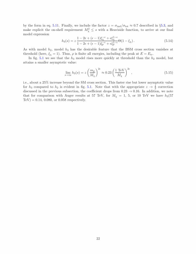
by the form in eq. 5.11. Finally, we include the factor z = σinel/σtot ≈ 0.7 described in §5.3, andmake explicit the on-shell requirement M2
χ ≤ s with a Heaviside function, to arrive at our finalmodel expression
h3(s) = z1− 2ǫ+ (ǫ− 1)ξ−ǫ
χ + ǫξ1−ǫχ
1− 2ǫ+ (ǫ− 1)ξ−ǫp + ǫξ1−ǫ
pΘ(1− ξχ) . (5.14)
As with model h2, model h3 has the desirable feature that the BSM cross section vanishes atthreshold (here, ξχ = 1). Thus, ρ is finite all energies, including the peak at E = Etr.
In fig. 5.1 we see that the h3 model rises more quickly at threshold than the h2 model, butattains a smaller asymptotic value:
lims→∞
h3(s) = z
(
mp
Mχ
)2ǫ
≈ 0.23
(
1 TeV
Mχ
)2ǫ
, (5.15)
i.e., about a 25% increase beyond the SM cross section. This faster rise but lower asymptotic valuefor h3 compared to h2 is evident in fig. 5.1. Note that with the appropriate z → 1
2 correctiondiscussed in the previous subsection, the coefficient drops from 0.23 → 0.16. In addition, we notethat for comparison with Auger results at 57 TeV, for Mχ = 1, 5, or 10 TeV we have h3(57TeV) = 0.14, 0.080, or 0.058 respectively.
22
Chapter 6
Results
For each of the three models discussed in chapter 5, we calculate the effect they have on ρ. Theparameter considered is the fractional increase in ρ, given as ∆ρ/ρ ≡ (ρ− ρSM)/ρSM. This is thenrelated to the TOTEM results at
√s = 7 TeV. We consider the mean value from their experiment
as an example signal: ρ = 0.145 (±0.091, 1σ confidence level) is compared to the SM predictionof ρ = 0.1345, a value which implies a fractional increase of ∆ρ/ρ = 0.0781. The error in thetheoretical calculation of ρ from existing measurements is < 1% [10]. This error is negligibly smallcompared to the effects presented here; we are justified in neglecting this error. We also look at theTOTEM upper limit, given as ρ < 0.32 at the 2σ confidence level, leading to a maximum fractionalincrease of ∆ρ/ρ < 1.38 (2σ).
In what follows we conservatively neglect the increase in the elastic cross section due to newphysics. This increase is model dependent. With the simplest assumptions, unitarity yields
σelσinel
=η
2− η, (6.1)
where 0 < η ≤ 1 is a measure of the absorption [54]. In general η may vary with the partial wavevalue J . We also note that η = 1 corresponds to the black disk limit, but the LHC is pre-asymptotic.
6.1 Results From the Step Function Model
The step function enhancement of ρ is shown in fig. 6.1. As expected, a shape very similar to thatof fig. 3.2 results. For comparison, the SM behavior of ρ is also shown. Here we have taken D = 1and
√str = 20 TeV. We see for a doubling of the cross section at
√str = 20 TeV, a small increase in
ρ is evident already at an energy an order of magnitude below√str = 20 TeV, and that ρ increases
by nearly a factor of four at√sobs = 14 TeV.
Next, we look at what range of√str and D values will give an large increase in ρ. The left
and right panels of fig. 6.2 show contours of ∆ρ/ρ in the ranges D ∈ [0, 1] and D ∈ [0, 10]. TheD ∈ [0, 1] range of the left panel may be relevant to broken R-parity violating SUSY-like models,in which some or all of the SM particles might be doubled. The larger D range is plotted in theright panel, to show the increased reach of IDRs for still larger cross sections, as might be the casewith extra-dimensional models. For the simple case of a step function with a significant increasein cross section, we see that IDRs offer a very powerful window to physics BSM.
Also displayed in fig. 6.2 are the regions of the generous h1 step function model that are ruledout at 95% significance by these TOTEM results. The IDR technique is sensitive to a large rangeof (
√str,D) parameter space of the h1 step function model, even with the currently large TOTEM
errors on the IDR independent ρ. In particular, the IDR technique is sensitive to new energythresholds well beyond the direct energy reach of the LHC. A minimal inference to be drawn fromthe 95% confidence level exclusion in the figure is that the cross section cannot increase particularlyquickly near the LHC energy
√s = 7 TeV.
Going forward, improvements are planned for the TOTEM optics, which will reduce the errorson ρ and thereby increase the sensitivity of the IDR toolkit to BSM physics.
Shown also in fig. 6.2 is the contour corresponding to our ρ = 0.145 example signal. Ourexample value of ρ is taken from the TOTEM experiment’s inferred mean value. If such a signal
23
104 105√sobs (GeV)
0.0
0.2
0.4
0.6
0.8
1.0
1.2
1.4
ρ
h0
h1√sthr = 20TeV
√sobs
0.0
0.5
1.0
1.5
2.0
2.5
ρ
h0
h1√sthr = 20TeV
Figure 6.1: At observational energies around LHC energies, the SM ρ (solid line) remains roughlyconstant. Using the step function enhancement h1 with D = 1 and
√str = 20 TeV, we find a
dramatic increase in ρ well below the new particle threshold. The right panel is an expanded pieceof the left panel with a width of ∼ 500 GeV on each side of the threshold energy, better showingthe asymmetry of ρ about its singular peak value.
1 5 7 10 50 100√sthr (TeV)
0.0
0.2
0.4
0.6
0.8
1.0
D
0.01
0.020.05
0.1
0.2
0.51
25
95%
example
1 5 7 10 50 100√sthr (TeV)
0
2
4
6
8
10
D
0.1
0.2
0.5
1
2
510
20
95%
example
Figure 6.2: At√sobs = 7 TeV, the contours are parameterized by ∆ρ/ρ. The form of the
enhancement that includes new physics is h1 – the step function. The left panel considers D in therange [0,1], which is the relevant parameter space for SUSY-type models. The right panel considersD values up to 10, relevant for extra-dimensional theories that have arbitrarily large increases inthe cross section. The shaded regions have already been ruled out by TOTEM’s
√s = 7 TeV
preliminary results. The dotted green contours correspond to the ρ = 0.145 example signal.
24

102 103 104 105
Mχ (GeV)
0.00
0.05
0.10
0.15
0.20
0.25
0.30
0.35
0.40
∆σ/σ
∆ρ/ρ
example
Figure 6.3: The fractional increases in ρ and σ using h2(s) at√sobs = 7 TeV, versus Mχ. With
the present significance of ρ data, the exclusion region is well above the top of the graph. Thelocation of the peak is determined by the pdfs. The dotted green line labeled example presents thevalue of ∆ρ/ρ corresponding to the ρ = 0.145 example signature; from intersecting lines, a newMχ = 5.1 TeV threshold is predicted.
were statistically and systematically significant, we would expect new physics to show up as anincrease in the pp cross section of height D and threshold
√str somewhere on this contour. (We
don’t consider a signal of new physics at energies much below the machine energy, as direct detectionof new event topologies or increased cross section would likely provide a better signal than a changein ρ as inferred through IDRs.)
We now turn to our more realistic models, h2 and h3, describing the onset of new physics. Theh1 model contains two parameters, D and Etr, and so for this model we showed the predictionfor ∆ρ/ρ as a contour plot. With the h2 and h3 models, there is no analog of D, and the onlyparameter is Etr. Thus, we may show ∆ρ/ρ and ∆σ/σ for these models as simple ordinates versusthe mass Mχ of the new particle, and we do so. With these models, our enthusiasm for the IDRapproach will be somewhat tempered.
6.2 Results From the Partonic Model
Results for the partonic h2 model are displayed in fig. 6.3, for future runs of the LHC at√s = 14
TeV.For a small range of Mχ values, it is seen that ∆ρ/ρ is significantly larger than ∆σ/σ. However,
at present, the errors on the IDR independent ρ measurement (∆ρ/ρ . 1.38 at 2σ) are much larger
25
than the accuracy (∼5%) with which energy-dependent changes in the total cross section can beinferred, so care is warranted here. From fig. 6.3 we can estimate a region of energy in the 2-5 TeVrange for which ∆ρ/ρ & 0.1 and ∆σ/σ . 0.05.
Our inference is that for new particle masses in the ∼2-5 TeV energy range, IDR independentmeasurements of ρ to an accuracy of one part in ten could reveal new physics of the type describedby h2 in section 5.3 at
√sobs = 7 TeV.
One may wonder why the peak in ρ occurs so far below the machine energy of 14 TeV. Thereason is the slow rise of the BSM cross section due to suppression from the pdfs: a peak at energyEtr ∼ √
s weighted by the mean value of the parton momenta product, 〈x1x2〉, gives a peak atroughly an order of magnitude below the machine energy. A second inference is that models withnew physics arising from initial state partons will enhance the value of ρ mainly below the machineenergy. Of course, such models will also enhance the cross section below the machine energy, asseen in fig. 6.3.
There is still a small increase in ρ at the machine energy of√str > 7 TeV due to particle masses
beyond 7 TeV. Beyond the machine energy, it is impossible for direct production to occur, so aninference of nonzero ∆ρ/ρ > 0 due to particle masses beyond
√str > 7 TeV would present a unique,
and striking, discovery. Unfortunately, in the h2 model, such an inference does not seem possible,as ∆ρ/ρ is . 0.01 for new particle masses just beyond 7 TeV. A more optimistic inference is that,if the cross section were to rise much more quickly than that of the h2 model, as happens witha Kaluza-Klein tower of new particles, it may be possible to infer such new physics even if thethreshold energies/new masses exceed the LHC energy.
We see that our example signal, plotted in fig. 6.3, implicates a new mass-scale Mχ = 5.1 TeV.(The example ∆ρ/ρ also crosses the continuous curve at an energy below the machine energy; weassume that any new physics at this lower energy would be detected through more direct means.)
6.3 Results From the Diffractive Model
Finally, the h3 model is plotted in fig. 6.4 at√sobs = 7 TeV. We see a modest contribution to
ρ from the h3 modification, as compared to that of the h2 model. The larger contribution is dueto the faster rise of the h3 model from threshold (str = M2
χ). The non-partonic nature of modelh3 is at the heart of the larger, higher-energy peak. On the other hand, the effect of the smallerincrease as s → ∞ as described by eq. 5.15 can be seen in fig. 6.4 by the fast fall off in ∆ρ/ρ beyond√s = Mχ.We note that while no regions of Mχ parameter space can yet be excluded, our example signal
implicates a new Mχ = 9.1 TeV mass-scale. (We again ignore the lower energy crossing, where anynew physics might be probed in a more direct manner.) This ∼ 9 TeV mass-scale has not beendirectly probed at the LHC, and likely will be only weakly probed even at the 14 TeV run.
26
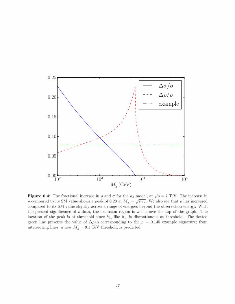
102 103 104 105
Mχ (GeV)
0.00
0.05
0.10
0.15
0.20
0.25
∆σ/σ
∆ρ/ρ
example
Figure 6.4: The fractional increase in ρ and σ for the h3 model, at√s = 7 TeV. The increase in
ρ compared to its SM value shows a peak of 0.23 at Mχ =√sobs. We also see that ρ has increased
compared to its SM value slightly across a range of energies beyond the observation energy. Withthe present significance of ρ data, the exclusion region is well above the top of the graph. Thelocation of the peak is at threshold since h3, like h1, is discontinuous at threshold. The dottedgreen line presents the value of ∆ρ/ρ corresponding to the ρ = 0.145 example signature; fromintersecting lines, a new Mχ = 9.1 TeV threshold is predicted.
27
Chapter 7
Conclusions
In the h1 and h3 models, the peak sensitivity of ∆ρ/ρ occurs when the new mass/new physicsthreshold is right at the machine energy. The sensitivity then falls off rapidly with increasingmass/threshold. However, the phase space for new particle production with mass at the machineenergy is zero. Thus, a cross section measurement will not show an increase for such a mass value.However, the ρ-parameter will show a peak increase. Thus, the IDR technique primarily extendsthe reach of the LHC, to particle masses at the very end point of the machine energy. The LHCdiscovery potential is also extended beyond the machine energy, but with less sensitivity. In theh2 model, the parton fractional momenta move the peak sensitivity to lower energies (by aboutan order of magnitude), thereby lessening the utility of the IDR technique for extending the LHCdiscovery potential to the machine energy and beyond.
It appears that this IDR technique may be sensitive to some reasonable models with largechanges to the pp cross section, which have thresholds exceeding the reach of more direct detection.
The outlook for the near future is dependent on new measurements of ρ from experiments likeTOTEM. The
√s = 8 TeV data from TOTEM is in the process of being analyzed [55], and we
eagerly await data from future LHC runs probing higher energies.
28

Appendix
A Minimum Transfer Energy in Two Lights to Light + One Heavy Processes
We need |t| small in h2 (see §5.3) to avoid amplitude suppression by propagators. Here we calculatethe kinematic range of t in the 2 → 2 process p1 + p2 → k1 + k2, with p21 = p22 = k22 = 0 all labelingSM particles and k21 = M2
χ labeling a new heavy particle. We will see that t = 0 is allowed, leadingto an unsuppressed amplitude for massless particle exchange.
Let θ be the angle between p1 and k1 in the COM frame. Then the transfer energy squared is
t = (p1 − k1)2 (A.1)
= M2χ − 2(p01k
01 − |p1| |k1| cos θ) , (A.2)
where k01 = k12 +M2
χ. So, tmax /min are given by
tmax /min = M2χ − 2p01k
01 ± 2|p1| |k1| , (A.3)
at θ = 0, π respectively. Then we have
p01 =
√s
2, k01 =
s+M2χ
2√s
, and (A.4)
|p1| = p01, |k1| =s−M2
χ
2√s
, and so (A.5)
p01k01 =
s+M2χ
4, |p1| |k1| =
s−M2χ
4. (A.6)
Then, the maximum/minimum values of t are
t = M2χ −
s+M2χ
2±
s−M2χ
2=
(
0
M2χ − s
)
, (A.7)
where t = 0 occurs for the forward scattering θ = 0 case, and the maximum |t| transfer occurs forthe backward scattering θ = π case. The tmin = 0 result confirms that pp → χ+light particles willfavor small |t|.
29

Part II
Ultra High Energy Cosmic Ray Anisotropy
30

Chapter 8
Introduction
8.1 Introduction
This part of the thesis is focused on ultra high energy cosmic ray (UHECR) anisotropy. A confer-ence proceeding outlining this work can be found at reference [2]. Two articles on this can be foundat references [3, 4]. The former of those two references is largely contained in chapter 12 while thelater contains the content in the remaining chapters. In the remainder of this chapter we will out-line the path of this part and motivate the study of UHECR anisotropy as well as discuss previousanisotropy searches. In chapter 9 we discuss the relevant modern UHECR experiments and theparameters used for the comparison between partial sky ground based experiments and space basedfull sky experiments. We present the tools we will be using to search for anisotropies in chapter 10.In chapter 11 we discuss the various approaches for reconstructing dipolar and quadrupolar aniso-tropies for experiments with full sky or partial sky exposure. Chapter 12 explains how anisotropieson certain scales, the quadrupole for the relevant experimental parameters, can be reconstrcutedfor ground based partial sky experiments while using the simpler and more accurate approachesdesigned only for space based full sky experiments. We discuss the difficulties of distinguishingbetween dipoles and quadrupoles with partial sky experiments and how they are resolved by fullsky experiments in chapter 13. Chapter 14 contains the results of the general comparison betweenfull sky and partial sky experiments and chapter 15 contains our conclusions.
8.2 Motivation
Pierre Auger kicked off the field of high energy cosmic ray research when he realized that extensiveair showers (EASs) implied the existence of very high energy cosmic rays in 1938 [56]. At thehighest energies, ∼ 1020 eV, the flux drops to about one event per square kilometer per century.Measuring this flux requires extremely large experiments as have been built and proposed, seechapter 9.
Despite measuring the cosmic ray flux up to and beyond energies of 1020 eV (1011 GeV, 100EeV), determining their properties has been less successful. It is unknown if the UHECRs6 areprotons or heavier nuclei [57, 58] or what their sources are. It is also unknown if the apparentsuppression that lines up with that predicted from the GZK phenomenon is, in fact, due to theGZK phenomenon or if sources naturally end at the same energy. The properties of galactic [59,60]and extragalactic magnetic fields [61] are also poorly understood with the latter being nearlycompletely unconstrained. Finally, the sources and acceleration methods of UHECRs are not yetunderstood and most models struggle to account for both the large maximum energy of UHECRsand the flux at those energies [62–67].
In light of this impressive list of unknowns, determining the sources of UHECRs is a top priorityin disentangling these related questions. Once the identification of UHECR sources is complete, thepath towards understanding the remaining questions will become more clear. To this end, however,little progress has been made. While Auger has noted some weakly significant signals [68], theircurrent status is unclear [69]. TA recently found a 20 “hotspot” [70] at global significance of
6UHECR typically means E & 1019 eV or so, although this varies in the literature.
31
3.4σ with an expanded data set. None of these analyses have yet identified the source of UHECRsdespite a plethora of different search techniques.
In this part, we take a simplifying approach. We attempt to maximize the ability for experimentsto identify any deviation from isotropy using a maximally generalized mathematical framework.We adopt spherical harmonics as a tool to identify anisotropies at varying scales and address thestrengths and weaknesses of them at partial sky ground based experiments and full sky space basedexperiments.
8.3 Previous Anisotropy Searches
No all sky observatory has yet flown. Consequently, the first full sky large anisotropy searchwas based on combined northern and southern hemisphere ground based data. The respectivedata came from the SUGAR [71] and AGASA [72] experiments, taken over a 10 year period. Nosignificant deviation from isotropy was seen by these experiments, even at energies beyond 4×10¹⁹
eV [73]. More recently, the Pierre Auger Collaboration carried out various searches for large scaleanisotropies in the distribution of arrival directions of cosmic rays above 1018 eV (an EeV) [74,75].At the energies exceeding 6 × 10¹⁹ eV = 60 EeV, early hints for a dipole anisotropy existed, butthese hints have grown increasingly weaker in statistical strength [76]. The latest Auger study wasperformed as a function of both declination and right ascension (RA) in several energy ranges above1018 eV. Their results were reported in terms of dipole and quadrupole amplitudes. Assuming thatany cosmic ray anisotropy is dominated by dipole and quadrupole moments in this energy range, thePierre Auger Collaboration derived upper limits on their amplitudes. Such upper limits challengean origin of cosmic rays above 1018 eV from long lived galactic sources densely distributed in thegalactic disk [77]. In the E > 8 EeV bin, they did report a dipolar signal with a p value of 6.4×10⁻⁵
(not including a “look elsewhere” penalty factor) [78]. Their cutoff of ∼ 8 EeV is above the galacticto extragalactic transition energy of ∼ 1 EeV, but still below the GZK cutoff energy of ∼ 55 EeV.Also, Telescope Array (TA), the largest cosmic ray experiment in the northern hemisphere, hasreported a different weak anisotropy signal above their highest energy cut of 57 EeV [70].
32
Chapter 9
Experiments
The Pierre Auger Observatory is an excellent, largest in its class, ground based experiment. How-ever, in the natural progression of science, it is expected that eventually ground based observationwill be superseded by space based observatories. The Extreme Universe Space Observatory (EUSO)is proposed to be the first of its class, space based observatory, building upon ground based successes.In this chapter we outline the relevant parameters of the two main ground based experiments, thePierre Auger Observatory and the Telescope Array, and a proposed space based experiment, theExtreme Universe Space Observatory.
9.1 Current Ground Based Experiments
The largest cosmic ray experiments currently are the Pierre Auger Observatory (Auger) and theTelescope Array (TA). These experiments will be the focus of this section.
9.1.1 Pierre Auger Observatory
The Pierre Auger Observatory (Auger) is situated in Argentina at 35.2S, 69.5W and is a hybriddetector designed to detect the extensive air showers (EASs) that result from the interaction ofUHECRs and air particles using the atmosphere as a calorimeter. The experiment is made up ofa surface detector (SD) and a fluorescence detector (FD). The SD is a collection of 1,600 tankscovering an area of 3,000 km2. As a useful comparison, this is roughly the size of the state ofRhode Island. The tanks of water are about a meter deep and a meter and a half in radiusto detect Cherenkov radiation charged particles with photomultiplier tubes and a reflective innersurface.
At about 1 km from the core of the EAS, muons saturate the signal, while the contribution fromphotons and electrons is negligible [79,80]. The FD is a collection of 24 telescopes positioned acrossfour sites overlooking the SD array. The FD is designed to measure the light yield from nitrogenfluorescence of EASs on dark moonless nights [81]. This provides a more accurate calorimetricmeasurement that is then used to calibrate the SD for the remaining of the data [79].
A major success of this experiment is the measurement of the flux suppression above ∼ 4×10¹⁹
eV due to the so called GZK7 phenomenon [82–84]. The focus of UHECR anisotropy is in lookingat the events with energies large enough that their sources must be relatively nearby due to theGZK phenomenon – this typically means with E & 55 EeV which implies d . 100 Mpc. Abovethese energies anisotropies are expected to appear.
9.1.2 Telescope Array
Telescope Array (TA) in Utah at 39.3N, 112.9W provides a northern hemisphere complement tothe southern hemisphere’s Auger. TA is also a hybrid detector with a similar FD design as Augerwith three sites each composed of multiple telescopes overlooking the SD array [85]. The TA SD
7The GZK process is where high energy protons lose energy when scattering off the cosmic microwave backgroundradiation (CMB), mainly resonantly through a ∆ baryon: p+γCMB → ∆ → N+π. There are also additional channelsfor protons to lose energy by scattering off the CMB, including higher ∆ resonances and alternate decay channelsthat typically include more pions.
33
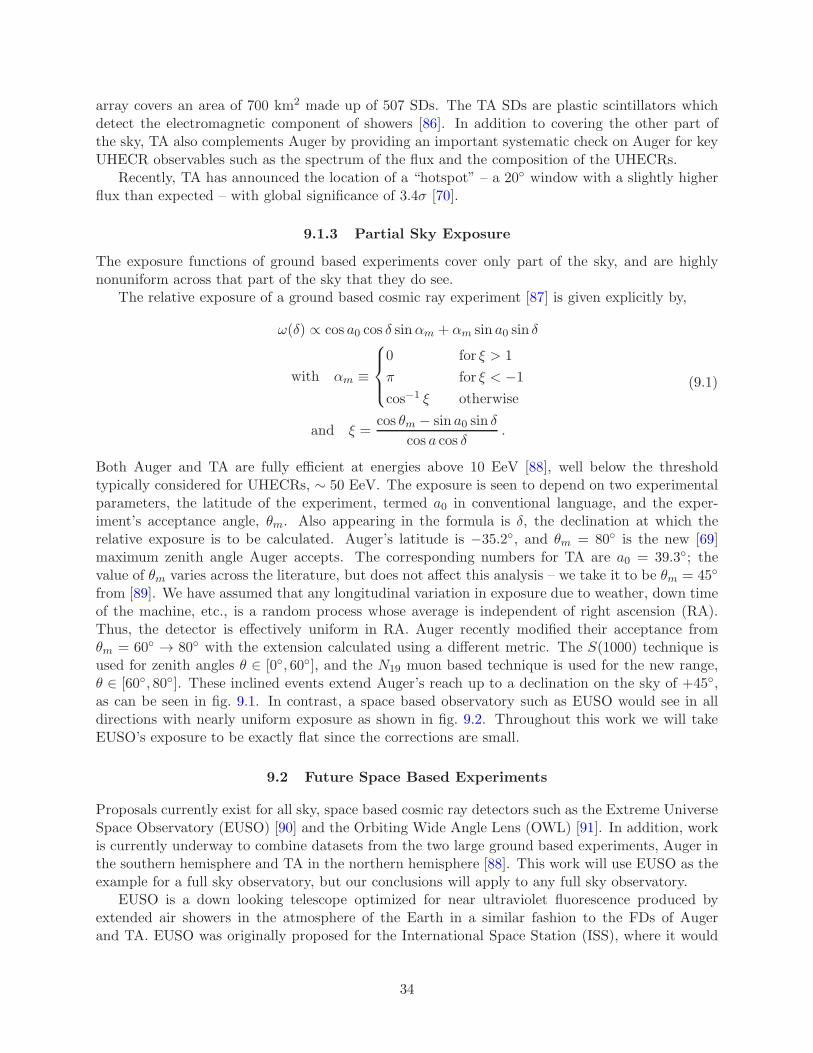
array covers an area of 700 km2 made up of 507 SDs. The TA SDs are plastic scintillators whichdetect the electromagnetic component of showers [86]. In addition to covering the other part ofthe sky, TA also complements Auger by providing an important systematic check on Auger for keyUHECR observables such as the spectrum of the flux and the composition of the UHECRs.
Recently, TA has announced the location of a “hotspot” – a 20 window with a slightly higherflux than expected – with global significance of 3.4σ [70].
9.1.3 Partial Sky Exposure
The exposure functions of ground based experiments cover only part of the sky, and are highlynonuniform across that part of the sky that they do see.
The relative exposure of a ground based cosmic ray experiment [87] is given explicitly by,
ω(δ) ∝ cos a0 cos δ sinαm + αm sin a0 sin δ
with αm ≡
0 for ξ > 1
π for ξ < −1
cos−1 ξ otherwise
and ξ =cos θm − sin a0 sin δ
cos a cos δ.
(9.1)
Both Auger and TA are fully efficient at energies above 10 EeV [88], well below the thresholdtypically considered for UHECRs, ∼ 50 EeV. The exposure is seen to depend on two experimentalparameters, the latitude of the experiment, termed a0 in conventional language, and the exper-iment’s acceptance angle, θm. Also appearing in the formula is δ, the declination at which therelative exposure is to be calculated. Auger’s latitude is −35.2, and θm = 80 is the new [69]maximum zenith angle Auger accepts. The corresponding numbers for TA are a0 = 39.3; thevalue of θm varies across the literature, but does not affect this analysis – we take it to be θm = 45
from [89]. We have assumed that any longitudinal variation in exposure due to weather, down timeof the machine, etc., is a random process whose average is independent of right ascension (RA).Thus, the detector is effectively uniform in RA. Auger recently modified their acceptance fromθm = 60 → 80 with the extension calculated using a different metric. The S(1000) technique isused for zenith angles θ ∈ [0, 60], and the N19 muon based technique is used for the new range,θ ∈ [60, 80]. These inclined events extend Auger’s reach up to a declination on the sky of +45,as can be seen in fig. 9.1. In contrast, a space based observatory such as EUSO would see in alldirections with nearly uniform exposure as shown in fig. 9.2. Throughout this work we will takeEUSO’s exposure to be exactly flat since the corrections are small.
9.2 Future Space Based Experiments
Proposals currently exist for all sky, space based cosmic ray detectors such as the Extreme UniverseSpace Observatory (EUSO) [90] and the Orbiting Wide Angle Lens (OWL) [91]. In addition, workis currently underway to combine datasets from the two large ground based experiments, Auger inthe southern hemisphere and TA in the northern hemisphere [88]. This work will use EUSO as theexample for a full sky observatory, but our conclusions will apply to any full sky observatory.
EUSO is a down looking telescope optimized for near ultraviolet fluorescence produced byextended air showers in the atmosphere of the Earth in a similar fashion to the FDs of Augerand TA. EUSO was originally proposed for the International Space Station (ISS), where it would
34
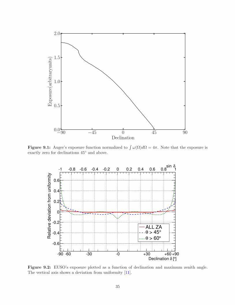
−90 −45 0 45 90Declination
0.0
0.5
1.0
1.5
2.0
Exp
osure(arbitraryunits)
Figure 9.1: Auger’s exposure function normalized to∫
ω(Ω)dΩ = 4π. Note that the exposure isexactly zero for declinations 45 and above.
1 0.8 0.6 0.4 0.2 0 0.2 0.4 0.6 0.8 1
Re
lative
de
via
tio
n f
rom
un
ifo
rmity
0.6
0.4
0.2
0
0.2
0.4
0.6
90 60 30 0 +30 +60 +90]° [δDeclination
δsin1 0.8 0.6 0.4 0.2 0 0.2 0.4 0.6 0.8 1
ALL ZA° > 45θ
° > 60θ
Figure 9.2: EUSO’s exposure plotted as a function of declination and maximum zenith angle.The vertical axis shows a deviation from uniformity [11].
35

collect up to 1000 cosmic ray events at and above 55 EeV (1 EeV = 1018 eV) over a 5 year lifetime,surpassing the reach of any ground based project.
It must be emphasized that because previous data from ground based experiments were sosparse at energies which would be accessible to EUSO, upper limits on anisotropy were necessarilyrestricted to energies below the threshold of EUSO. EUSO expects many more events at ∼ 1020
eV, allowing an enhanced anisotropy reach. In addition, EUSO would observe more events with ahigher rigidity R = E/Z, events less bent by magnetic fields which may be helpful in identifyingpoint sources on the sky.
EUSO brings two new, major advantages to the search for the origins of UHECRs. One advan-tage is the large field of view (FOV), attainable only with a space based observatory. With a 60
opening angle for the telescope, the down pointing (“nadir”) FOV is
π(hISS tan(30))2 ≈ h2ISS ≈ 150, 000 km2 . (9.2)
We will compare the ability to detect large scale anisotropies at a space based, full sky exper-iment with that of a ground based partial sky experiment. For reference, we will use the largestground based cosmic ray observatory, Auger [92]. Thus the proposed EUSO FOV, given in eq. 9.2, is50 times larger for instantaneous measurements (e.g., for observing transient sources). Multiplyingthe proposed EUSO FOV by an expected 18% duty cycle, yields a time averaged nine fold increasein acceptance for the EUSO design compared to Auger, at energies where the EUSO efficiency haspeaked (at and above & 50−100 EeV). Tilting the telescope turns the circular FOV given in eq. 9.2into a larger elliptical FOV. The price paid for “tilt mode” is an increase in the threshold energyof the experiment.
The second advantage of a space based experiment over a ground based one is the coverageof the full sky (4π steradians) with nearly constant exposure and consistent systematic errors onthe energy and angle resolution, again attainable only with a space based observatory. This partcompares full sky studies of possible anisotropies to partial sky studies. The reach benefits fromthe 4π sky coverage, but also from the increased statistics resulting from the greater FOV.
9.3 Event Rates
The 231 event sample published by Auger over 9.25 years of recording cosmic rays at and above∼ 52 EeV [69] allows us to estimate the flux at these energies. The annual rate of such events atAuger is ∼ 231/9.25 = 25. For simplicity, we consider a 250 event sample for Auger, as might becollected over a full decade.
Including the suppressed efficiency of EUSO down to ∼ 55 EeV reduces the factor of 9 relativeto Auger down to a factor ∼6 for energies at and above 55 EeV. We arrive at the 450 event sampleas the EUSO expectation at and above 55 EeV after three years running in nadir mode (or, as isunder discussion, in tilt mode with an increased aperture but a reduced number of photons). A 750event sample is then expected for five years of EUSO running in a combination of nadir and tiltmode. Finally, the event rate at an energy measured by TA is known to significantly exceed thatof Auger. This leads to a five year event rate at EUSO of about 1000 events. Thus, we considerthe motivated data samples of 250, 450, 750, and 1000 events in the simulations that follow.
36
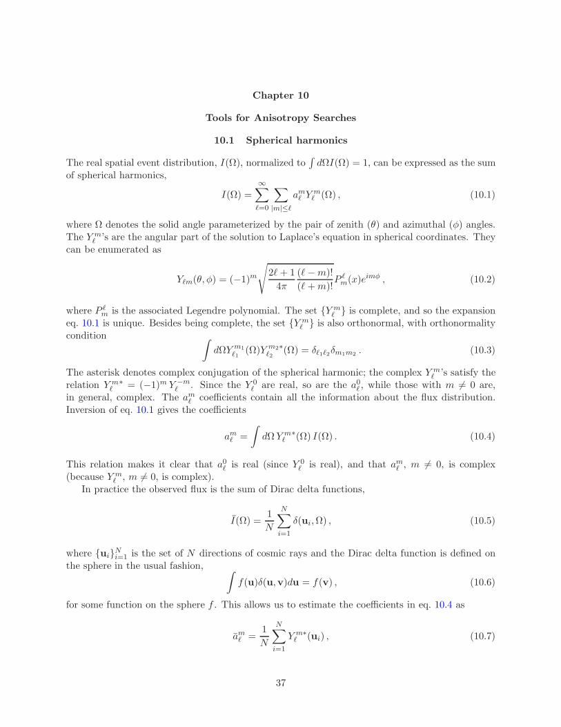
Chapter 10
Tools for Anisotropy Searches
10.1 Spherical harmonics
The real spatial event distribution, I(Ω), normalized to∫
dΩI(Ω) = 1, can be expressed as the sumof spherical harmonics,
I(Ω) =∞∑
ℓ=0
∑
|m|≤ℓ
amℓ Y mℓ (Ω) , (10.1)
where Ω denotes the solid angle parameterized by the pair of zenith (θ) and azimuthal (φ) angles.The Y m
ℓ ’s are the angular part of the solution to Laplace’s equation in spherical coordinates. Theycan be enumerated as
Yℓm(θ, φ) = (−1)m
√
2ℓ+ 1
4π
(ℓ−m)!
(ℓ+m)!P ℓm(x)eimφ , (10.2)
where P ℓm is the associated Legendre polynomial. The set Y m
ℓ is complete, and so the expansioneq. 10.1 is unique. Besides being complete, the set Y m
ℓ is also orthonormal, with orthonormalitycondition
∫
dΩY m1
ℓ1(Ω)Y m2∗
ℓ2(Ω) = δℓ1ℓ2δm1m2
. (10.3)
The asterisk denotes complex conjugation of the spherical harmonic; the complex Y mℓ ’s satisfy the
relation Y mℓ
∗ = (−1)m Y −mℓ . Since the Y 0
ℓ are real, so are the a0ℓ , while those with m 6= 0 are,in general, complex. The amℓ coefficients contain all the information about the flux distribution.Inversion of eq. 10.1 gives the coefficients
amℓ =
∫
dΩY mℓ
∗(Ω) I(Ω) . (10.4)
This relation makes it clear that a0ℓ is real (since Y 0ℓ is real), and that amℓ , m 6= 0, is complex
(because Y mℓ , m 6= 0, is complex).
In practice the observed flux is the sum of Dirac delta functions,
I(Ω) =1
N
N∑
i=1
δ(ui,Ω) , (10.5)
where uiNi=1 is the set of N directions of cosmic rays and the Dirac delta function is defined onthe sphere in the usual fashion,
∫
f(u)δ(u,v)du = f(v) , (10.6)
for some function on the sphere f . This allows us to estimate the coefficients in eq. 10.4 as
amℓ =1
N
N∑
i=1
Y m∗ℓ (ui) , (10.7)
37
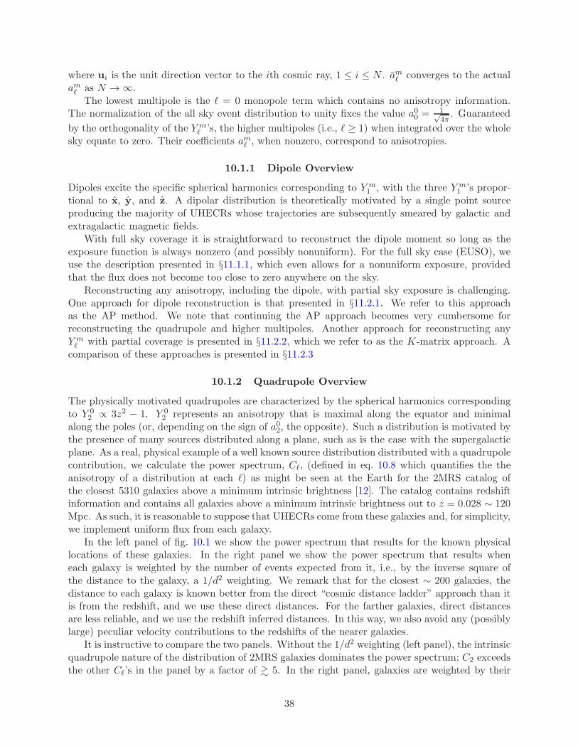
where ui is the unit direction vector to the ith cosmic ray, 1 ≤ i ≤ N . amℓ converges to the actualamℓ as N → ∞.
The lowest multipole is the ℓ = 0 monopole term which contains no anisotropy information.The normalization of the all sky event distribution to unity fixes the value a00 = 1√
4π. Guaranteed
by the orthogonality of the Y mℓ ’s, the higher multipoles (i.e., ℓ ≥ 1) when integrated over the whole
sky equate to zero. Their coefficients amℓ , when nonzero, correspond to anisotropies.
10.1.1 Dipole Overview
Dipoles excite the specific spherical harmonics corresponding to Y m1 , with the three Y m
1 ’s propor-tional to x, y, and z. A dipolar distribution is theoretically motivated by a single point sourceproducing the majority of UHECRs whose trajectories are subsequently smeared by galactic andextragalactic magnetic fields.
With full sky coverage it is straightforward to reconstruct the dipole moment so long as theexposure function is always nonzero (and possibly nonuniform). For the full sky case (EUSO), weuse the description presented in §11.1.1, which even allows for a nonuniform exposure, providedthat the flux does not become too close to zero anywhere on the sky.
Reconstructing any anisotropy, including the dipole, with partial sky exposure is challenging.One approach for dipole reconstruction is that presented in §11.2.1. We refer to this approachas the AP method. We note that continuing the AP approach becomes very cumbersome forreconstructing the quadrupole and higher multipoles. Another approach for reconstructing anyY mℓ with partial coverage is presented in §11.2.2, which we refer to as the K-matrix approach. A
comparison of these approaches is presented in §11.2.3
10.1.2 Quadrupole Overview
The physically motivated quadrupoles are characterized by the spherical harmonics correspondingto Y 0
2 ∝ 3z2 − 1. Y 02 represents an anisotropy that is maximal along the equator and minimal
along the poles (or, depending on the sign of a02, the opposite). Such a distribution is motivated bythe presence of many sources distributed along a plane, such as is the case with the supergalacticplane. As a real, physical example of a well known source distribution distributed with a quadrupolecontribution, we calculate the power spectrum, Cℓ, (defined in eq. 10.8 which quantifies the theanisotropy of a distribution at each ℓ) as might be seen at the Earth for the 2MRS catalog ofthe closest 5310 galaxies above a minimum intrinsic brightness [12]. The catalog contains redshiftinformation and contains all galaxies above a minimum intrinsic brightness out to z = 0.028 ∼ 120Mpc. As such, it is reasonable to suppose that UHECRs come from these galaxies and, for simplicity,we implement uniform flux from each galaxy.
In the left panel of fig. 10.1 we show the power spectrum that results for the known physicallocations of these galaxies. In the right panel we show the power spectrum that results wheneach galaxy is weighted by the number of events expected from it, i.e., by the inverse square ofthe distance to the galaxy, a 1/d2 weighting. We remark that for the closest ∼ 200 galaxies, thedistance to each galaxy is known better from the direct “cosmic distance ladder” approach than itis from the redshift, and we use these direct distances. For the farther galaxies, direct distancesare less reliable, and we use the redshift inferred distances. In this way, we also avoid any (possiblylarge) peculiar velocity contributions to the redshifts of the nearer galaxies.
It is instructive to compare the two panels. Without the 1/d2 weighting (left panel), the intrinsicquadrupole nature of the distribution of 2MRS galaxies dominates the power spectrum; C2 exceedsthe other Cℓ’s in the panel by a factor of & 5. In the right panel, galaxies are weighted by their
38
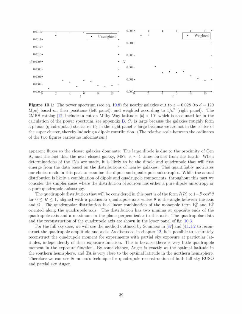
0 2 4 6 8 10ℓ
0.0000
0.0002
0.0004
0.0006
0.0008
0.0010
0.0012
0.0014
0.0016C
ℓ
Unweighted
0 2 4 6 8 10ℓ
0.000
0.001
0.002
0.003
0.004
0.005
Cℓ
Weighted
Figure 10.1: The power spectrum (see eq. 10.8) for nearby galaxies out to z = 0.028 (to d = 120Mpc) based on their positions (left panel), and weighted according to 1/d2 (right panel). The2MRS catalog [12] includes a cut on Milky Way latitudes |b| < 10 which is accounted for in thecalculation of the power spectrum, see appendix B. C2 is large because the galaxies roughly forma planar (quadrupolar) structure; C1 in the right panel is large because we are not in the center ofthe super cluster, thereby inducing a dipole contribution. (The relative scale between the ordinatesof the two figures carries no information.)
apparent fluxes so the closest galaxies dominate. The large dipole is due to the proximity of CenA, and the fact that the next closest galaxy, M87, is ∼ 4 times farther from the Earth. Whendeterminations of the Cℓ’s are made, it is likely to be the dipole and quadrupole that will firstemerge from the data based on the distributions of nearby galaxies. This quantifiably motivatesour choice made in this part to examine the dipole and quadrupole anisotropies. While the actualdistribution is likely a combination of dipole and quadrupole components, throughout this part weconsider the simpler cases where the distribution of sources has either a pure dipole anisotropy ora pure quadrupole anisotropy.
The quadrupole distribution that will be considered in this part is of the form I(Ω) ∝ 1−B cos2 θfor 0 ≤ B ≤ 1, aligned with a particular quadrupole axis where θ is the angle between the axisand Ω. The quadrupolar distribution is a linear combination of the monopole term Y 0
0 and Y 02
oriented along the quadrupole axis. The distribution has two minima at opposite ends of thequadrupole axis and a maximum in the plane perpendicular to this axis. The quadrupolar dataand the reconstruction of the quadrupole axis are shown in the lower panel of fig. 10.3.
For the full sky case, we will use the method outlined by Sommers in [87] and §11.1.2 to recon-struct the quadrupole amplitude and axis. As discussed in chapter 12, it is possible to accuratelyreconstruct the quadrupole moment for experiments with partial sky exposure at particular lat-itudes, independently of their exposure function. This is because there is very little quadrupolemoment in the exposure function. By some chance, Auger is exactly at the optimal latitude inthe southern hemisphere, and TA is very close to the optimal latitude in the northern hemisphere.Therefore we can use Sommers’s technique for quadrupole reconstruction of both full sky EUSOand partial sky Auger.
39

Figure 10.2: Nodal lines separating excess and deficit regions of sky for various (ℓ,m) pairs. Thetop row shows the (0, 0) monopole, and the partition of the sky into two dipoles, (1, 0) and (1, 1).The middle row shows the quadrupoles (2, 0), (2, 1), and (2, 2). The bottom row shows the ℓ = 3partitions, (3, 0), (3, 1), (3, 2), and (3, 3).
10.2 Power Spectrum
The power spectrum is defined as
Cℓ ≡1
2ℓ+ 1
ℓ∑
m=−ℓ
|amℓ |2 , (10.8)
The following subsections discuss various properties of the power spectrum.
10.2.1 Nodal Lines
A Y mℓ with a nonzero m corresponds to 2 |m| longitudinal “slices” (|m| nodal meridians) on the
sky. There are ℓ − |m| + 1 latitudinal “zones” (ℓ − |m| nodal latitudes). In fig. 10.2 we show thepartitioning described by some low multipole moments. Useful visualizations of spherical harmonicscan also be found in [93]. The configurations with (ℓ,−|m|) are related to those with (ℓ,+|m|) bya longitudinal phase advance φ ⇒ φ+ π
2 , or cosφ ⇒ sinφ.A simple approximation for the number of cosmic rays necessary to resolve power at a particular
level is to count the number NZ(ℓ,m) of nodal zones in each Y mℓ . Each Y m
ℓ has
NZ(ℓ,m) =
ℓ+ 1 m = 0
2|m|(ℓ− |m|+ 1) m 6= 0, (10.9)
nodal zones. The average over m of the number nodal zones at a given ℓ is,
〈NZ(ℓ)〉 =ℓ+ 1
3(2ℓ+ 1)(2ℓ2 + 4ℓ+ 3) . (10.10)
For low values of ℓ, this returns the obvious results,
〈NZ(ℓ = 0)〉 = 1 , 〈NZ(ℓ = 1)〉 = 2 . (10.11)
40

For large ℓ,
〈NZ(ℓ)〉 →ℓ2
3. (10.12)
If we make the simple assumption of requiring O(1) event per nodal zone to resolve a particularterm in the power spectrum, then, for large ℓ we require ∼ ℓ2/3 events to resolve Cℓ. Thus, the ruleof thumb is that our EUSO fiducial samples of 450, 750, and 1000 events can resolve the Cℓ’s upto an ℓ value of the mid 30’s, mid 40’s, and mid 50’s, respectively, i.e., (using θ ∼ 90
ℓ ) can resolvestructures on the sky down to 2− 3. A ground based observatory, due to having fewer events andno full sky coverage, would do much worse. We note that the statistical error in angle estimatedhere for EUSO event numbers is well matched to the expected systematic angular resolution error∼ 1 of EUSO.
10.2.2 Proof of the Rotational Invariance of the Power Spectrum
While calculating the coefficients of the spherical harmonics, the amℓ ’s, is useful, the amℓ ’s sufferthe disadvantage that they are frame dependent. The spherical harmonics coefficients, the amℓ ’sgiven in eq. 10.1, are clearly coordinate dependent, as a simple rotation in the φ coordinate willchange the eimφ part of the spherical harmonic for m 6= 0, and a rotation in the θ coordinate willchange the associated Legendre polynomial part Pm
ℓ (θ) for ℓ 6= 0. So only the ℓ = m = 0 monopolecoefficient is coordinate independent.
To combat this problem of rotational noninvariance of the spherical harmonic coefficients, weturn to the power spectrum, defined in eq. 10.8. While it may be intuitive that the Cℓ should berotationally (coordinate) invariant, this attribute is not obvious. The purpose of this subsection isto prove the rotational invariance of the power spectrum.
For a discrete set of sources, the normalized intensity function is given by eq. 10.5. In terms ofspherical harmonics, one finds that the spherical harmonic coefficients are given by eq. 10.7 whereui is the unit direction vector to the ith cosmic ray, 1 ≤ i ≤ N .
To construct the estimation of the associated power spectrum, we square these amℓ ’s followedby a sum over m:
Cℓ ≡1
2ℓ+ 1
∑
|m|≤ℓ
|amℓ |2
=1
N2(2ℓ+ 1)
∑
|m|≤ℓ
∣
∣
∣
∣
∣
N∑
i=1
Y m∗ℓ (ui)
∣
∣
∣
∣
∣
2
.
(10.13)
Since the sums are finite they may be rearranged and expanded to
Cℓ =1
N2(2ℓ+ 1)
N∑
i=1
∑
|m|≤ℓ
|Y mℓ (ui)|2 ++
2
N2(2ℓ+ 1)
∑
i<j
∑
|m|≤ℓ
Y m∗ℓ (ui)Y
mℓ (uj) . (10.14)
The addition formula [94] for spherical harmonics is
Pℓ(x · y) = 4π
2ℓ+ 1
∑
|m|≤ℓ
Y m∗ℓ (x)Y m
ℓ (y) , (10.15)
where Pℓ(cos θ) is the Legendre polynomial. Since Pℓ(1) = 1, setting the unit direction vectors x
and y to be equal in eq. 10.15, one gets
2ℓ+ 1
4π=∑
|m|≤ℓ
|Y mℓ (x)|2 . (10.16)
41
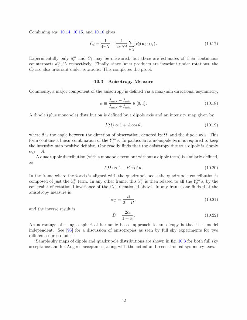
Combining eqs. 10.14, 10.15, and 10.16 gives
Cℓ =1
4πN+
1
2πN2
∑
i<j
Pℓ(ui · uj) . (10.17)
Experimentally only amℓ and Cℓ may be measured, but these are estimates of their continuouscounterparts amℓ , Cℓ respectively. Finally, since inner products are invariant under rotations, theCℓ are also invariant under rotations. This completes the proof.
10.3 Anisotropy Measure
Commonly, a major component of the anisotropy is defined via a max/min directional asymmetry,
α ≡ Imax − Imin
Imax + Imin∈ [0, 1] . (10.18)
A dipole (plus monopole) distribution is defined by a dipole axis and an intensity map given by
I(Ω) ∝ 1 +A cos θ , (10.19)
where θ is the angle between the direction of observation, denoted by Ω, and the dipole axis. Thisform contains a linear combination of the Y m
1 ’s. In particular, a monopole term is required to keepthe intensity map positive definite. One readily finds that the anisotropy due to a dipole is simplyαD = A.
A quadrupole distribution (with a monopole term but without a dipole term) is similarly defined,as
I(Ω) ∝ 1−B cos2 θ . (10.20)
In the frame where the z axis is aligned with the quadrupole axis, the quadrupole contribution iscomposed of just the Y 0
2 term. In any other frame, this Y 02 is then related to all the Y m
2 ’s, by theconstraint of rotational invariance of the Cℓ’s mentioned above. In any frame, one finds that theanisotropy measure is
αQ =B
2−B, (10.21)
and the inverse result is
B =2α
1 + α. (10.22)
An advantage of using a spherical harmonic based approach to anisotropy is that it is modelindependent. See [95] for a discussion of anisotropies as seen by full sky experiments for twodifferent source models.
Sample sky maps of dipole and quadrupole distributions are shown in fig. 10.3 for both full skyacceptance and for Auger’s acceptance, along with the actual and reconstructed symmetry axes.
42

60S
30S
0
30N
60N
60S
30S
0
30N
60N
60S
30S
0
30N
60N
60S
30S
0
30N
60N
Figure 10.3: Shown are sample sky maps of 500 cosmic rays. The top row corresponds to theαD,true = 1 dipole, while the bottom row corresponds to the αQ,true = 1 quadrupole distribution.The left and right panels correspond to all sky, space based and partial sky, ground based coverage,respectively. The injected dipole or quadrupole axis is shown as a blue diamond, and the recon-structed direction is shown as a red star. We see that reconstruction of the multipole directionwith an event number of 500 is excellent for an all sky observatory (left panels) and quite goodfor partial sky Auger (right panels). In practice, αD and αQ are likely much less than unity, andthe event rate for all sky EUSO is expected to be ∼ 9 times that of Auger. Both effects on thecomparison of Auger and EUSO are shown in figs. 14.1 and 14.2.
43
Chapter 11
Reconstructing Anisotropies
Detecting any deviation from isotropy in UHECRs has been a long sought after goal. For example,at high energies above the GZK suppression, the anisotropies are expected to reveal the distributionof cosmic ray sources among nearby galaxies. One common approach for measuring anisotropies isto partition the sky into regions of various sizes with the use of spherical harmonics. The low orderspherical harmonics correspond to simple structures. The lowest nontrivial order, ℓ = 1, called thedipole, may correspond to a single source where the cosmic rays have been smeared out by magneticfields during propagation. The next order, ℓ = 2, called the quadrupole, can correspond to a planardistribution of sources, such as might be the case if the sources are spread across the galacticor supergalactic plane. Unfortunately partial sky experiments cannot, in principle, distinguishbetween dipoles and quadrupoles. For example, Auger would see a dipole with a maximum towardsthe north pole as a band of maxima along the equator and would be indistinguishable from a planarquadrupole with the same axis.
11.1 Full Sky Coverage
Reconstructing the spherical harmonics in general, including the quadrupole anisotropy magnitudearising from a planar distribution of sources, is straightforward with full sky (even nonuniform)coverage. In this section we will explain the standard approaches in the literature for reconstructingthe ℓ = 1, 2 spherical harmonics with full sky coverage. We also present a new approach forreconstructing a quadrupole with either full or partial sky coverage that is more transparent thanthe standard approach.
11.1.1 Sommers’s Approach for Dipoles
P. Sommers presented a straightforward approach to reconstruct dipolar anisotropies with full skycoverage but possibly nonuniform exposure, hereafter referred to as Sommers’s approach [87]. GivenN events at directions u(i) with relative exposures ωi at each event, under the assumption that ωis zero nowhere on the sphere, the dipole anisotropy magnitude and direction is given simply by
αDDa =3
NN∑
i=1
1
ωiu(i)a , (11.1)
where i ∈ x, y, z, D is the unit vector in the dipole direction, and
N =
N∑
i=1
1
ωi, (11.2)
is the appropriate normalization factor given the relative exposure.
11.1.2 Sommers’s Approach for Quadrupoles
P. Sommers also presented an approach to reconstruct quadrupolar anisotropies with full sky cov-erage but possibly nonuniform exposure, hereafter referred to as Sommers’s approach [87]. He
44
presents his quadrupolar matrix,
Sab =
∫
I(Ω)uaubdΩ , (11.3)
with a, b ∈ x, y, z, so ua is a particular component of u. For discrete sources, this can be estimatedin the typical fashion,
Sab =1
NN∑
i=1
1
ω(ui)u(i)a u
(i)b , (11.4)
with N given by eq. 11.2. Then, for λ1 < λ2 < λ3 the eigenvalues of S,
∆ =λ2 + λ3
2− λ1 , ξ =
2− 10∆
2 + 5∆. (11.5)
Finally, the anisotropy from a quadrupolar distribution is given by,
αQ =1− ξ
1 + ξ. (11.6)
11.1.3 New Approach for Quadrupoles
Sommers outlines one method for calculating the anisotropy from a pure quadrupolar distribution[87] as discussed in §11.1.2. His approach assumes full sky (possibly nonuniform) exposure. Basedon the results from chapter 12, that same approach can be applied for Auger and TA by ignoringtheir exposure.
Since the power spectrum is rotationally invariant as shown in §10.2.2, we can consider a newalternate derivation of the quadrupole strength. Begin by choosing a coordinate frame that alignsthe z-axis with the symmetry axis of the quadrupole. Then only a00 and a02 are nonzero.
In terms of Cartesian coordinates,
Y 02 = A(3z2 − 1) , (11.7)
with A = 14
√
5π . The intensity function in Cartesian coordinates aligned with the quadrupole axis
isI = B(1− Cz2) , (11.8)
where the normalization requirement sets 1B = 4π(1 − C
3 ). We then invert eq. 11.7 to write theintensity as a function of Y 0
0 and Y 02 .
I =1√4π
Y 00 − BC
3AY 02 . (11.9)
In the coordinate frame where the quadrupole symmetry axis is aligned with the z axis, only a00and a02 are nonzero and are given by eq. 11.9. Then a02 = −
√5C2 where we used the definition of
the power spectrum from eq. 10.8 and the sign is because a02 in eq. 11.9 is negative definite. Thisform is reminiscient of some aspects of that presented by Sommers in §11.1.2.
Then we have a new prescription to find αQ as defined in eq. 10.18. First calculate the powerspectrum for ℓ = 2 in any coordinate frame for data with either full sky coverage or from experimentsat latitudes 30 . |a0| . 40 (see chapter 12 for further discussion on reconstructing quadrupoleswith partial sky exposure). Then get a02 and then find C as described in eq. 11.9 and this gives αQ
from eq. 12.21.
45
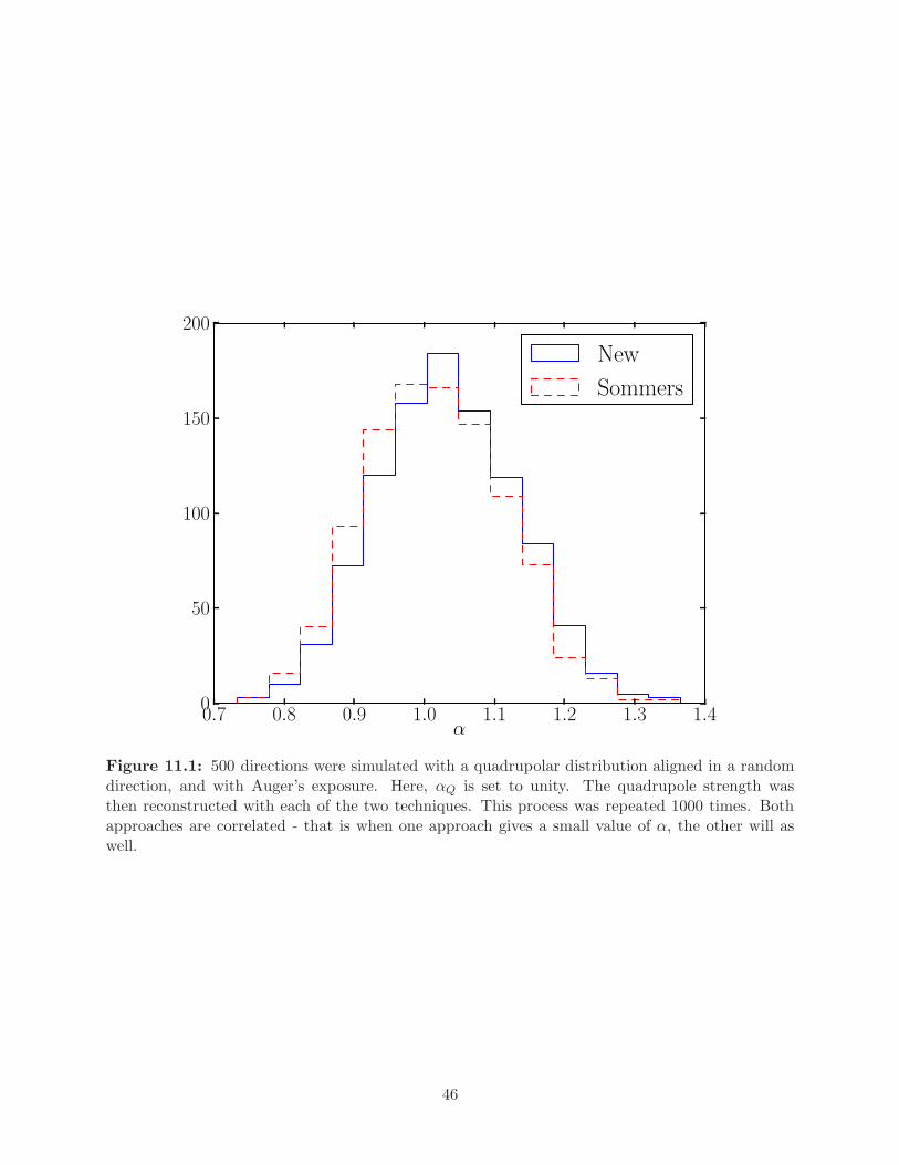
0.7 0.8 0.9 1.0 1.1 1.2 1.3 1.4α
0
50
100
150
200
New
Sommers
Figure 11.1: 500 directions were simulated with a quadrupolar distribution aligned in a randomdirection, and with Auger’s exposure. Here, αQ is set to unity. The quadrupole strength wasthen reconstructed with each of the two techniques. This process was repeated 1000 times. Bothapproaches are correlated - that is when one approach gives a small value of α, the other will aswell.
46
We compare this approach to that described by Sommers in [87]. We note that this newtechnique does not provide directional information, which is available in the eigenvectors of the Qtensor as described by Sommers. A plot of the comparison is shown in fig. 11.1 of the reconstructedquadrupole amplitude. The results are consistent with each other. In particular, the means andstandard deviation for each approach are 1.033 ± 0.099 for this new approach and 1.017 ± 0.098for Sommers’s approach, compared to a correct value of 1. The nonnegligible deviations in thereconstructed values are not due to the small corrections mentioned in eq. 12.19, rather they aredue to the fact that a discrete sampling with finite N number of delta functions of a continuousdistribution tends to lend itself to larger anisotropies. Nonetheless, this approach has value due toits straightforward derivation from the power spectrum.
11.2 Partial Sky Coverage
Reconstructing spherical harmonics with partial sky coverage complicates things dramatically com-pared to the full sky case. While the techniques in the literature for dealing with the dipole onpartial sky coverage are fairly simple, those for a quadrupole are not [75, 96, 97]. In this sectionwe present two approaches for reconstructing dipoles with partial sky coverage and a comparisonof the two. We present no approach for reconstructing the quadrupole with partial sky coveragebecause we will show in chapter 12 that either of the full sky approaches presented can be used forpartial sky due to the particular locations of the two ground based UHECR experiments.
11.2.1 AP Approach for Dipoles
J. Aublin and E. Parizot presented one approach for reconstructing dipoles with partial sky an-isotropy, hereafter referred to as the AP approach [98]. We summarize the AP approach in thissubsection. They made the important observation that the nonuniformity of the exposure functionof ground based experiments is much less important than the regions where it is zero.
They begin by defining a number of useful intermediate variables.
d = cos θmin − cos θmax , (11.10)
s = cos θmin + cos θmax , (11.11)
p = cos θmin × cos θmax , (11.12)
γ =s2 − p
3, (11.13)
where θmin = 90−θm−a0 and θmax = 90. Next, they calculate the zeroth and first order momentsof the flux.
I0 =
∫ θmax
θmin
dθ sin θ
∫ 2π
0dφΦ(u) , (11.14)
I =
∫ θmax
θmin
dθ sin θ
∫ 2π
0dφuΦ(u) . (11.15)
47
From this they invert and find that the dipole magnitude and direction is given by
αDDx =Ix
sIz − 2γI0
γ − p
γ − 1, (11.16)
αDDy =Iy
sIz − 2γI0
γ − p
γ − 1, (11.17)
αDDz =sI0 − 2IzsIz − 2γI0
. (11.18)
This approach provided a significant improvement over the standard at the time, which was a onedimensional Rayleigh analysis which discards all declination information [99].
11.2.2 K-matrix Approach
P. Billoir and O. Deligny present an approach to reconstruct anisotropies of any order hereafterreferred to as the K-matrix approach [97]. They begin by writing down the K-matrix for a givenexposure function (generally defined for ground based experiments in eq. 9.1),
[K]mm′
ℓℓ′ =
∫
dΩY mℓ (Ω)ω(Ω)Y m′
ℓ′ . (11.19)
This matrix describes how the exposure function ω causes the various spherical harmonics tointerfere. From this the uncorrected spherical harmonic coefficients observed at a ground basedexperiment,
bmℓ =
∫
dΩY m∗ℓ (Ω)ω(Ω)I(Ω) , (11.20)
can be exactly related to the true spherical harmonic coefficients,
amℓ =
∫
dΩY m∗ℓ (Ω)I(Ω) , (11.21)
by the relation
bmℓ =∑
ℓ′,m′
[K]mm′
ℓℓ′ am′
ℓ′ . (11.22)
Of course, we are interested in turning uncorrected coefficients into true coefficients which involvesinverting an infinite matrix. To this end, an ℓmax must be introduced to truncate the matrix. Thisapproach is completely generalizable to calculate any ℓ. Once the estimate of the true coefficientsare acquired, the anisotropy measure can be calculated using either Sommers’s approach for full skydiscussed in §11.1.1 for dipoles or the new approach presented in §11.1.3 for quadrupoles, althoughwe will show in chapter 12 that the K-matrix step can be skipped for partial sky experimentswith certain experimental parameters, which both Auger and TA satisfy when they are measuringquadrupoles. A numerical comparison of this approach applied to reconstructing dipoles and theAP approach presented in §11.2.1 is presented in §11.2.3.
11.2.3 Comparison of Partial Sky Dipole Approaches
§11.2.1 and §11.2.2 present the AP and K-matrix approaches, respectively, for reconstructingdipoles measured at a ground based partial sky experiment. We compare these two approaches todetermine which optimally reconstructs a given dipole distribution. Our result is most clearly pre-sented in fig. 11.2. We consider 500 cosmic rays with a dipole distribution of magnitude αD,true = 1
48
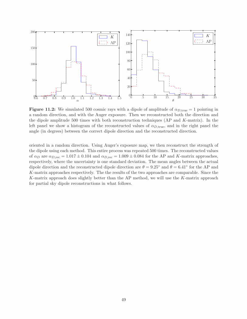
0.6 0.7 0.8 0.9 1.0 1.1 1.2 1.3 1.4 1.5α
0
50
100
150
200
K
AP
0 5 10 15 20 25 30 35θ
0
20
40
60
80
100
120
140 K
AP
Figure 11.2: We simulated 500 cosmic rays with a dipole of amplitude of αD,true = 1 pointing ina random direction, and with the Auger exposure. Then we reconstructed both the direction andthe dipole amplitude 500 times with both reconstruction techniques (AP and K-matrix). In theleft panel we show a histogram of the reconstructed values of αD,true, and in the right panel theangle (in degrees) between the correct dipole direction and the reconstructed direction.
oriented in a random direction. Using Auger’s exposure map, we then reconstruct the strength ofthe dipole using each method. This entire process was repeated 500 times. The reconstructed valuesof αD are αD,rec = 1.017± 0.104 and αD,rec = 1.009± 0.084 for the AP and K-matrix approaches,respectively, where the uncertainty is one standard deviation. The mean angles between the actualdipole direction and the reconstructed dipole direction are θ = 9.25 and θ = 6.41 for the AP andK-matrix approaches respectively. The the results of the two approaches are comparable. Since theK-matrix approach does slightly better than the AP method, we will use the K-matrix approachfor partial sky dipole reconstructions in what follows.
49
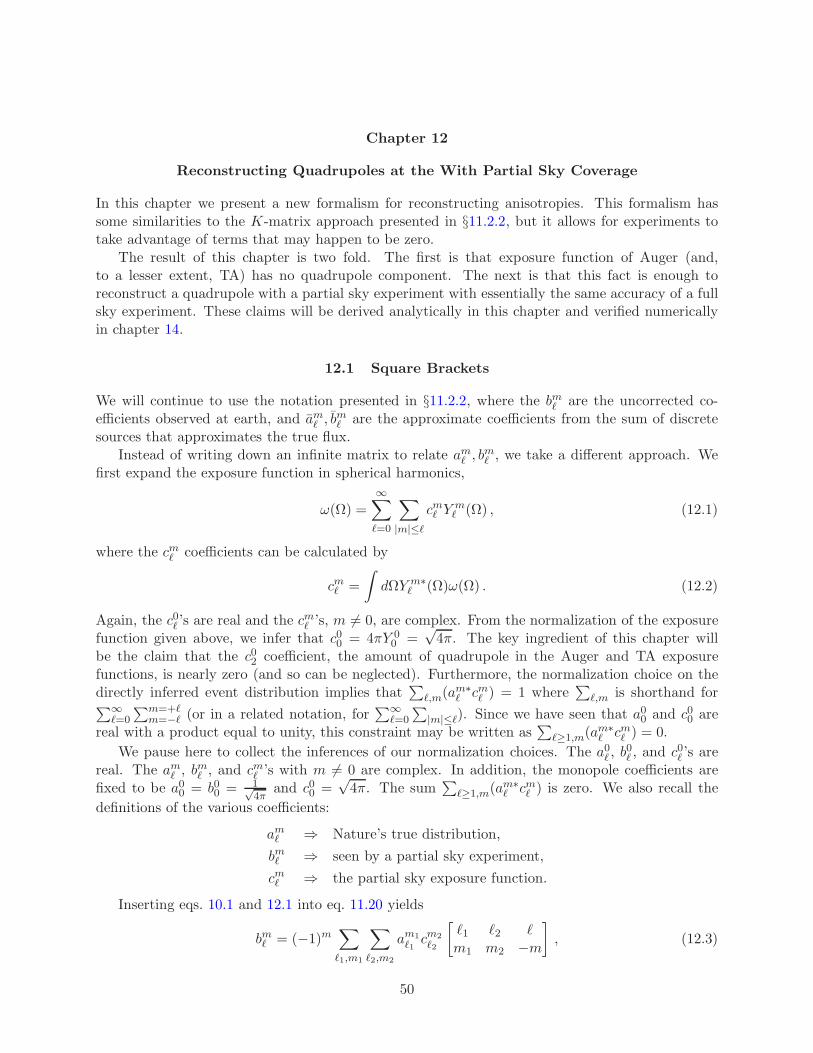
Chapter 12
Reconstructing Quadrupoles at the With Partial Sky Coverage
In this chapter we present a new formalism for reconstructing anisotropies. This formalism hassome similarities to the K-matrix approach presented in §11.2.2, but it allows for experiments totake advantage of terms that may happen to be zero.
The result of this chapter is two fold. The first is that exposure function of Auger (and,to a lesser extent, TA) has no quadrupole component. The next is that this fact is enough toreconstruct a quadrupole with a partial sky experiment with essentially the same accuracy of a fullsky experiment. These claims will be derived analytically in this chapter and verified numericallyin chapter 14.
12.1 Square Brackets
We will continue to use the notation presented in §11.2.2, where the bmℓ are the uncorrected co-efficients observed at earth, and amℓ , bmℓ are the approximate coefficients from the sum of discretesources that approximates the true flux.
Instead of writing down an infinite matrix to relate amℓ , bmℓ , we take a different approach. Wefirst expand the exposure function in spherical harmonics,
ω(Ω) =∞∑
ℓ=0
∑
|m|≤ℓ
cmℓ Y mℓ (Ω) , (12.1)
where the cmℓ coefficients can be calculated by
cmℓ =
∫
dΩY m∗ℓ (Ω)ω(Ω) . (12.2)
Again, the c0ℓ ’s are real and the cmℓ ’s, m 6= 0, are complex. From the normalization of the exposurefunction given above, we infer that c00 = 4πY 0
0 =√4π. The key ingredient of this chapter will
be the claim that the c02 coefficient, the amount of quadrupole in the Auger and TA exposurefunctions, is nearly zero (and so can be neglected). Furthermore, the normalization choice on thedirectly inferred event distribution implies that
∑
ℓ,m(am∗ℓ cmℓ ) = 1 where
∑
ℓ,m is shorthand for∑∞
ℓ=0
∑m=+ℓm=−ℓ (or in a related notation, for
∑∞ℓ=0
∑
|m|≤ℓ). Since we have seen that a00 and c00 arereal with a product equal to unity, this constraint may be written as
∑
ℓ≥1,m(am∗ℓ cmℓ ) = 0.
We pause here to collect the inferences of our normalization choices. The a0ℓ , b0ℓ , and c0ℓ ’s are
real. The amℓ , bmℓ , and cmℓ ’s with m 6= 0 are complex. In addition, the monopole coefficients arefixed to be a00 = b00 = 1√
4πand c00 =
√4π. The sum
∑
ℓ≥1,m(am∗ℓ cmℓ ) is zero. We also recall the
definitions of the various coefficients:
amℓ ⇒ Nature’s true distribution,
bmℓ ⇒ seen by a partial sky experiment,
cmℓ ⇒ the partial sky exposure function.
Inserting eqs. 10.1 and 12.1 into eq. 11.20 yields
bmℓ = (−1)m∑
ℓ1,m1
∑
ℓ2,m2
am1
ℓ1cm2
ℓ2
[
ℓ1 ℓ2 ℓm1 m2 −m
]
, (12.3)
50
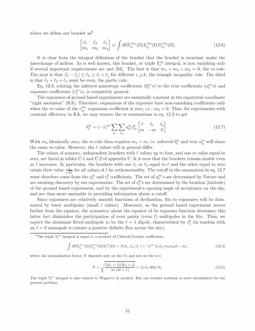
where we define our bracket as8
[
ℓ1 ℓ2 ℓ3m1 m2 m3
]
≡∫
dΩY m1
ℓ1(Ω)Y m2
ℓ2(Ω)Y m3
ℓ3(Ω) . (12.6)
It is clear from the integral definition of the bracket that the bracket is invariant under theinterchange of indices. As is well known, this bracket, or triple Y m
ℓ integral, is non vanishing onlyif several important requirements are met [94]. The first is that m1 + m2 + m3 = 0, the m-rule.The next is that |ℓi − ℓj | ≤ ℓk ≤ ℓi + ℓj for different i, j, k, the triangle inequality rule. The thirdis that ℓ1 + ℓ2 + ℓ3 must be even, the parity rule.
Eq. 12.3, relating the inferred anisotropy coefficients (bmℓ ’s) to the true coefficients (amℓ ’s) andexposure coefficients (cmℓ ’s), is completely general.
The exposures of ground based experiments are essentially constant in the equatorial coordinate“right ascension” (RA). Therefore, expansions of the exposure have non-vanishing coefficients onlywhen the m-value of the cm2
ℓ2expansion coefficient is zero, i.e., m2 = 0. Thus, for experiments with
constant efficiency in RA, we may remove the m summations in eq. 12.3 to get
bmℓ = (−1)m∑
ℓ1
∑
ℓ2
amℓ1c0ℓ2
[
ℓ ℓ1 ℓ2m −m 0
]
. (12.7)
With m2 identically zero, the m-rule then requires m1 = m, i.e. inferred bmℓ and true amℓ1 will sharethe same m-value. However, the ℓ values will in general differ.
The values of nonzero, independent brackets with ℓ values up to four, and one m value equal tozero, are listed in tables C.1 and C.2 of appendix C. It is seen that the brackets remain sizable evenas ℓ increases. In particular, the brackets with one ℓ1 or ℓ2 equal to ℓ and the other equal to zeroretain their value 1√
4πfor all values of ℓ by orthonormality. The cutoff in the summation in eq. 12.7
must therefore come from the amℓ and c0ℓ coefficients. The set of amℓ ’s are determined by Nature andare awaiting discovery by our experiments. The set of c0ℓ ’s are determined by the location (latitude)of the ground based experiment, and by the experiment’s opening angle of acceptance on the sky,and are thus more amenable to providing information about a cutoff.
Since exposures are relatively smooth functions of declination, fits to exposures will be dom-inated by lower multipoles (small ℓ values). Moreover, as the ground based experiment movesfarther from the equator, the symmetry about the equator of its exposure function decreases; thislatter fact diminishes the participation of even parity (even ℓ) multipoles in the fits. Thus, weexpect the dominant fitted multipole to be the ℓ = 1 dipole, characterized by c01 (in tandem withan ℓ = 0 monopole to ensure a positive definite flux across the sky).
8The triple Y mℓ integral is equal to a product of Clebsch-Gordan coefficients,
∫
dΩY m1
ℓ1(Ω)Y m2
ℓ2(Ω)Y m
ℓ (Ω) = N(ℓ1, ℓ2, ℓ)× (−1)m 〈ℓ1ℓ2;m1m2|ℓ;−m〉 , (12.4)
where the normalization factor N depends only on the ℓ’s and not on the m’s
N =
√
(2ℓ1 + 1)(2ℓ2 + 1)
4π (2ℓ+ 1)× 〈ℓ1ℓ2; 00|ℓ; 0〉 . (12.5)
The triple Y mℓ integral is also related to Wigner’s 3j symbol. But our bracket notation is more streamlined for the
present problem.
51
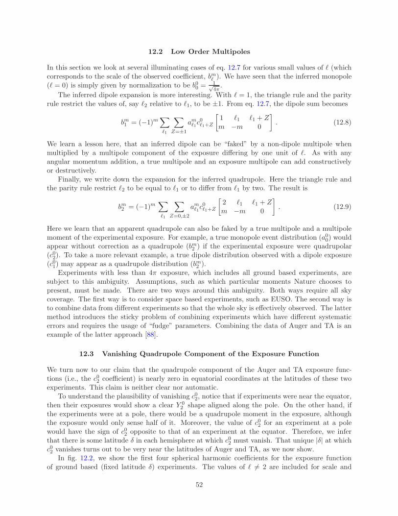
12.2 Low Order Multipoles
In this section we look at several illuminating cases of eq. 12.7 for various small values of ℓ (whichcorresponds to the scale of the observed coefficient, bmℓ ). We have seen that the inferred monopole(ℓ = 0) is simply given by normalization to be b00 =
1√4π.
The inferred dipole expansion is more interesting. With ℓ = 1, the triangle rule and the parityrule restrict the values of, say ℓ2 relative to ℓ1, to be ±1. From eq. 12.7, the dipole sum becomes
bm1 = (−1)m∑
ℓ1
∑
Z=±1
amℓ1c0ℓ1+Z
[
1 ℓ1 ℓ1 + Zm −m 0
]
. (12.8)
We learn a lesson here, that an inferred dipole can be “faked” by a non-dipole multipole whenmultiplied by a multipole component of the exposure differing by one unit of ℓ. As with anyangular momentum addition, a true multipole and an exposure multipole can add constructivelyor destructively.
Finally, we write down the expansion for the inferred quadrupole. Here the triangle rule andthe parity rule restrict ℓ2 to be equal to ℓ1 or to differ from ℓ1 by two. The result is
bm2 = (−1)m∑
ℓ1
∑
Z=0,±2
amℓ1c0ℓ1+Z
[
2 ℓ1 ℓ1 + Zm −m 0
]
. (12.9)
Here we learn that an apparent quadrupole can also be faked by a true multipole and a multipolemoment of the experimental exposure. For example, a true monopole event distribution (a00) wouldappear without correction as a quadrupole (bm2 ) if the experimental exposure were quadrupolar(c02). To take a more relevant example, a true dipole distribution observed with a dipole exposure(c01) may appear as a quadrupole distribution (bm2 ).
Experiments with less than 4π exposure, which includes all ground based experiments, aresubject to this ambiguity. Assumptions, such as which particular moments Nature chooses topresent, must be made. There are two ways around this ambiguity. Both ways require all skycoverage. The first way is to consider space based experiments, such as EUSO. The second way isto combine data from different experiments so that the whole sky is effectively observed. The lattermethod introduces the sticky problem of combining experiments which have different systematicerrors and requires the usage of “fudge” parameters. Combining the data of Auger and TA is anexample of the latter approach [88].
12.3 Vanishing Quadrupole Component of the Exposure Function
We turn now to our claim that the quadrupole component of the Auger and TA exposure func-tions (i.e., the c02 coefficient) is nearly zero in equatorial coordinates at the latitudes of these twoexperiments. This claim is neither clear nor automatic.
To understand the plausibility of vanishing c02, notice that if experiments were near the equator,then their exposures would show a clear Y 0
2 shape aligned along the pole. On the other hand, ifthe experiments were at a pole, there would be a quadrupole moment in the exposure, althoughthe exposure would only sense half of it. Moreover, the value of c02 for an experiment at a polewould have the sign of c02 opposite to that of an experiment at the equator. Therefore, we inferthat there is some latitude δ in each hemisphere at which c02 must vanish. That unique |δ| at whichc02 vanishes turns out to be very near the latitudes of Auger and TA, as we now show.
In fig. 12.2, we show the first four spherical harmonic coefficients for the exposure functionof ground based (fixed latitude δ) experiments. The values of ℓ 6= 2 are included for scale and
52
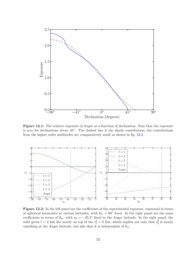
−90 −45 0 45 90
Declination (degrees)
0.0
0.5
1.0
1.5
2.0
2.5
Exp
osure
Figure 12.1: The relative exposure of Auger as a function of declination. Note that the exposureis zero for declinations above 45. The dashed line is the dipole contribution; the contributionsfrom the higher order multipoles are comparatively small as shown in fig. 12.2.
−90 −80 −70 −60 −50 −40 −30 −20 −10 0a0
−5
−4
−3
−2
−1
0
1
2
3
c0 ℓ
ℓ = 1
ℓ = 2
ℓ = 3
ℓ = 4
Auger
20 30 40 50 60 70 80 90θm
−4
−3
−2
−1
0
1
2
3
4
c0 ℓ
ℓ = 1
ℓ = 2
ℓ = 3
ℓ = 4
Auger
Figure 12.2: In the left panel are the coefficients of the experimental exposure, expressed in termsof spherical harmonics at various latitudes, with θm = 60 fixed. In the right panel are the samecoefficients in terms of θm, with a0 = −35.2 fixed to the Auger latitude. In the right panel, thesolid green ℓ = 2 line lies nearly on top of the c0ℓ = 0 line, which implies not only that c02 is nearlyvanishing at the Auger latitude, but also that it is independent of θm.
53

comparison. The left panel plots the first four c0ℓ coefficients versus the experimental latitude a0, indegrees. It is seen that the ±latitude for which c02 vanishes agrees very accurately with the latitudesof Auger and TA. In fact, Auger’s latitude is −35.21 (termed a0 in conventional notation), whilethe unique latitude at which c02 vanishes is −35.26. The difference between these two latitudes is∼ 7 km – much smaller than the scale of Auger. That is, the latitude at which c02 vanishes runsright through Auger.
It is also seen that the higher ℓ coefficients are small. The values of the fitted coefficients c00,c01, c
02, c
03, and c04 at the Auger latitude, and with the Auger opening angle of 80, are
√4π, −2.42,
−0.003, 0.019, and 0.218, respectively.The dependence on the acceptance angle θm is shown in the right panel of fig. 12.2. Note that
the c02 curve is zero to within the line thickness of the plot for all θm. It is seen that variations inthis angle does not affect this vanishing of c02 at the Auger latitude.
At Auger’s latitude, we see that the largest exposure coefficient in magnitude is c01, and that itis negative. This agrees with the expectation from fig. 12.1, which appears to be largely dipolar inNature. (We also note that at the equator c01 vanished, while c02 is large as expected. We brieflycomment on this case in §12.8.)
A conceptual complication is that the exposure function is necessarily evaluated in equatorialcoordinates, while anisotropies of interest are best considered in galactic coordinates. Any rotationin coordinates mixes the set of (2ℓ + 1) Y m
ℓ ’s with fixed ℓ. However, it is possible to reconstructanisotropy information in the coordinate frame of one’s choosing by using the rotationally invariant(see §10.2.2) power spectrum defined in eq. 10.8.
12.4 A Simplifying Cutoff
Armed with the result that the Auger exposure is dominantly dipole (c01) in shape, with a for-tuitously small quadrupole (c02 ≪ c01), and small higher multipoles, we expand the dipole andquadrupole sums up to order ℓ2 = 2. This is high enough order to reveal the gift that comes withthe justified neglect of c02 for Auger and TA.
Applying a cutoff at ℓ2 = 2 in the expansion of the exposure function, eqs. 12.8, and 12.9 are
bm1 = δm0c014π
+ am1 + (−1)m
am1 c02
[
1 1 2m −m 0
]
+am2 c01
[
1 2 1m −m 0
]
+ am3 c02
[
1 3 2m −m 0
]
, (12.10)
and
bm2 = δm0c024π
+ am2 + (−1)m
am1 c01
[
2 1 1m −m 0
]
+ am2 c02
[
2 2 2m −m 0
]
+ am3 c01
[
2 3 1m −m 0
]
+am4 c02
[
2 4 2m −m 0
]
. (12.11)
With |c02(δ, θm)| set to its minimum value of zero, a very good approximation for the latitudesof Auger and TA, we get
bm1 = δm0c014π
+ am1 + (−1)mam2 c01
[
1 2 1m −m 0
]
, (12.12)
54
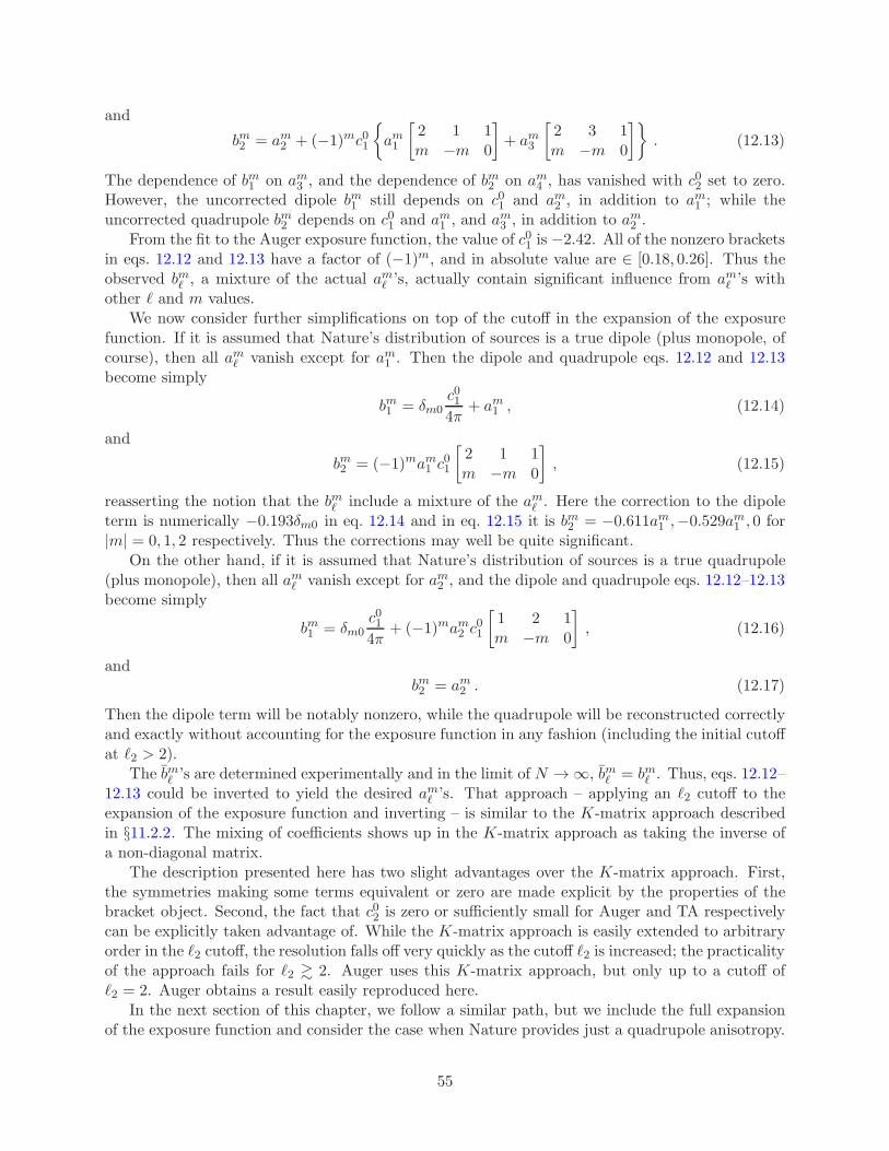
and
bm2 = am2 + (−1)mc01
am1
[
2 1 1m −m 0
]
+ am3
[
2 3 1m −m 0
]
. (12.13)
The dependence of bm1 on am3 , and the dependence of bm2 on am4 , has vanished with c02 set to zero.However, the uncorrected dipole bm1 still depends on c01 and am2 , in addition to am1 ; while theuncorrected quadrupole bm2 depends on c01 and am1 , and am3 , in addition to am2 .
From the fit to the Auger exposure function, the value of c01 is −2.42. All of the nonzero bracketsin eqs. 12.12 and 12.13 have a factor of (−1)m, and in absolute value are ∈ [0.18, 0.26]. Thus theobserved bmℓ , a mixture of the actual amℓ ’s, actually contain significant influence from amℓ ’s withother ℓ and m values.
We now consider further simplifications on top of the cutoff in the expansion of the exposurefunction. If it is assumed that Nature’s distribution of sources is a true dipole (plus monopole, ofcourse), then all amℓ vanish except for am1 . Then the dipole and quadrupole eqs. 12.12 and 12.13become simply
bm1 = δm0c014π
+ am1 , (12.14)
and
bm2 = (−1)mam1 c01
[
2 1 1m −m 0
]
, (12.15)
reasserting the notion that the bmℓ include a mixture of the amℓ . Here the correction to the dipoleterm is numerically −0.193δm0 in eq. 12.14 and in eq. 12.15 it is bm2 = −0.611am1 ,−0.529am1 , 0 for|m| = 0, 1, 2 respectively. Thus the corrections may well be quite significant.
On the other hand, if it is assumed that Nature’s distribution of sources is a true quadrupole(plus monopole), then all amℓ vanish except for am2 , and the dipole and quadrupole eqs. 12.12–12.13become simply
bm1 = δm0c014π
+ (−1)mam2 c01
[
1 2 1m −m 0
]
, (12.16)
andbm2 = am2 . (12.17)
Then the dipole term will be notably nonzero, while the quadrupole will be reconstructed correctlyand exactly without accounting for the exposure function in any fashion (including the initial cutoffat ℓ2 > 2).
The bmℓ ’s are determined experimentally and in the limit of N → ∞, bmℓ = bmℓ . Thus, eqs. 12.12–12.13 could be inverted to yield the desired amℓ ’s. That approach – applying an ℓ2 cutoff to theexpansion of the exposure function and inverting – is similar to the K-matrix approach describedin §11.2.2. The mixing of coefficients shows up in the K-matrix approach as taking the inverse ofa non-diagonal matrix.
The description presented here has two slight advantages over the K-matrix approach. First,the symmetries making some terms equivalent or zero are made explicit by the properties of thebracket object. Second, the fact that c02 is zero or sufficiently small for Auger and TA respectivelycan be explicitly taken advantage of. While the K-matrix approach is easily extended to arbitraryorder in the ℓ2 cutoff, the resolution falls off very quickly as the cutoff ℓ2 is increased; the practicalityof the approach fails for ℓ2 & 2. Auger uses this K-matrix approach, but only up to a cutoff ofℓ2 = 2. Auger obtains a result easily reproduced here.
In the next section of this chapter, we follow a similar path, but we include the full expansionof the exposure function and consider the case when Nature provides just a quadrupole anisotropy.
55
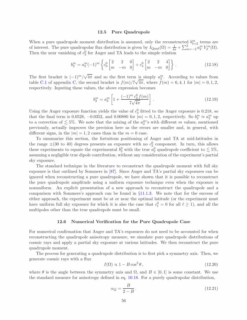
12.5 Pure Quadrupole
When a pure quadrupole moment distribution is assumed, only the reconstructed bmℓ=2 terms areof interest. The pure quadrupolar flux distribution is given by IQuad(Ω) =
14π +
∑2m=−2 a
m2 Y m
2 (Ω).Then the near vanishing of c02 for Auger and TA leads to the simple relation
bm2 = am2 (−1)m
c00
[
2 2 0m −m 0
]
+ c04
[
2 2 4m −m 0
]
. (12.18)
The first bracket is (−1)m/√4π and so the first term is simply am2 . According to values from
table C.1 of appendix C, the second bracket is f(m)/7√4π, where f(m) = 6, 4, 1 for |m| = 0, 1, 2,
respectively. Inputing these values, the above expression becomes
bm2 = am2
[
1 +(−1)m c04 f(m)
7√4π
]
. (12.19)
Using the Auger exposure function yields the value of c04 fitted to the Auger exposure is 0.218, sothat the final term is 0.0528, −0.0352, and 0.00880 for |m| = 0, 1, 2, respectively. So bm2 ≈ am2 upto a correction of . 5%. We note that the mixing of the am2 ’s with different m values, mentionedpreviously, actually improves the precision here as the errors are smaller and, in general, withdifferent signs, in the |m| = 1, 2 cases than in the m = 0 case.
To summarize this section, the fortuitous positioning of Auger and TA at mid-latitudes inthe range ±(30 to 40) degrees presents an exposure with no c02 component. In turn, this allowsthese experiments to equate the experimental b02 with the true a02 quadrupole coefficient to . 5%,assuming a negligible true dipole contribution, without any consideration of the experiment’s partialsky exposure.
The standard technique in the literature to reconstruct the quadrupole moment with full skyexposure is that outlined by Sommers in [87]. Since Auger and TA’s partial sky exposures can beignored when reconstructing a pure quadrupole, we have shown that it is possible to reconstructthe pure quadrupole amplitude using a uniform exposure technique even when the exposure isnonuniform. An explicit presentation of a new approach to reconstruct the quadrupole and acomparison with Sommers’s approach can be found in §11.1.3. We note that for the success ofeither approach, the experiment must be at or near the optimal latitude (or the experiment musthave uniform full sky exposure for which it is also the case that c0ℓ = 0 for all ℓ ≥ 1), and all themultipoles other than the true quadrupole must be small.
12.6 Numerical Verification for the Pure Quadrupole Case
For numerical confirmation that Auger and TA’s exposures do not need to be accounted for whenreconstructing the quadrupole anisotropy measure, we simulate pure quadrupole distributions ofcosmic rays and apply a partial sky exposure at various latitudes. We then reconstruct the purequadrupole moment.
The process for generating a quadrupole distribution is to first pick a symmetry axis. Then, wegenerate cosmic rays with a flux
I(Ω) ∝ 1−B cos2 θ , (12.20)
where θ is the angle between the symmetry axis and Ω, and B ∈ [0, 1] is some constant. We usethe standard measure for anisotropy defined in eq. 10.18. For a purely quadrupolar distribution,
αQ =B
2−B. (12.21)
56
0.0 0.1 0.2 0.3 0.4 0.5 0.6 0.7 0.8 0.9 1.0αQ,true
0.0
0.2
0.4
0.6
0.8
1.0
1.2
1.4
αQ,rec
−60.0
−45.0
−35.2
0.0
39.3
Figure 12.3: Quadrupoles with magnitudes shown on the horizontal axis are injected into anexperiment at the shown latitudes. The error bars for the inferred quadrupoles correspond to onestandard deviation over 500 repetitions with a different symmetry axis in each repetition. Theblack line is αQ,rec = αQ,true. The behavior of the inference at a0 = −35.2 away from the line atlow values of αQ,true is due to random fluctuations. The horizontal shift within one value of αQ,true
for different latitudes is implemented for clarity only.
The reconstructed pure quadrupole magnitude is shown in fig. 12.3 for several true quadrupolemagnitudes and several latitudes. In each simulation, a symmetry axis was randomly chosen. Then500 cosmic rays were distributed according to the quadrupolar distribution and the experiment’sexposure at the given latitude. This process was repeated 500 times and the mean and standarddeviation is shown. We see that a0 = −35.2 (Auger) reconstructs the quadrupole well. In addition,a0 = 39.3 (TA) reconstructs the quadrupole well (but slightly less so than |a0| = 35.2). In betweenthe two optimal latitudes, a0 = ±35.2, we see that the ability to simply reconstruct the quadrupolemoment vanishes by the large discrepancy in the a0 = 0 reconstruction attempts. In addition,locating the experiments closer to the poles also nullifies this effect as seen in the a0 = −60 case.Finally, at a0 = −45 we see how this effect begins to fall off as we move outside the 30 . |a0| . 40
region.
12.7 A Quadrupole Purity Test
In order to determine if a measured quadrupole is pure or if it is tainted by the other sphericalharmonics, we propose a simple statistical test. We only consider contamination from the ℓ = 1dipole contribution. For a given reconstructed αQ we want to know that the dipole amplitude αD,
57
0.0 0.1 0.2 0.3 0.4 0.5αD,true
0.0
0.1
0.2
0.3
0.4
0.5
Figure 12.4: Distributions with 500 cosmic rays, Auger’s exposure, maximal quadrupolar an-isotropy, and varying dipolar anisotropies were simulated. αD was then reconstructed using theK-matrix approach. Plotted on the vertical axis is the fraction of simulations with αD,rec notconsistent with zero at a 95% confidence level.
our test statistic, is small.We simulated 500 cosmic rays with Auger’s exposure and maximal quadrupole anisotropy,
αQ = 1. We then added in increasing amounts of dipole contribution, αD and reconstructed αD
using the K-matrix approach defined in §11.2.2. After repeating this process 10,000 times wecounted how often αD,rec was greater than the 95% limit for the αD = 0 pure quadrupole case. Theresults are shown in fig. 12.4.
For example, for a dipole contribution corresponding to αD = 0.5 compared with αQ = 1, thereis a 49% chance that αD = 0 could be rejected at the 95% confidence level. As the contaminatingdipole gets weaker, so does this probability.
We see that, as we expected, it is not particularly easy to determine if a quadrupole is pure ornot with partial sky coverage. As shown in eqs. 12.12–12.13, a quadrupolar signal may mimic adipolar signal and vice versa.
12.8 Pure Dipole
For completeness, we address the pure dipole analogy to the pure quadrupole discussion of §12.5.When a pure dipole distribution is assumed, we have IDipole =
14π +
∑1m=−1 a
m1 Y m
1 (Ω). Then the
58
near vanishing of c02 reduces eq. 12.10 to simply
bm1 = δm0c014π
+ am1 , (12.22)
the same result as in the ℓ2 cutoff case shown in eq. 12.14. In the pure quadrupole case, we foundthat bm2 was equal to am2 times a multiplicative factor that was within a few percent of unity. Herewe find the equality between am1 and bm1 is exact for m 6= 0, but is broken by an additive factor form = 0. The additive factor is neither large nor small, but rather it is −0.193. This additive factorwill also show up with the same relative strength in the power spectrum coefficient C1.
Referring back to fig. 12.2, one sees that an experiment near the equator would have vanishingc0ℓ ’s except for the quadrupole c02 ∼ −1.08. It is amusing to ask what pure dipole reconstructionmight be possible with such an experimental location. Eq. 12.22 is replaced with the followingequation:
bm1 = am1
1 + (−1)mc02
[
1 1 2m −m 0
]
= am1 [1 + 0.14(1 − 3δm0)] .
(12.23)
Unfortunately, the multiplicative correction from the now nonzero c02 coefficient is large.
59
Chapter 13
Distinguishing Between Dipoles and Quadrupoles
One topic of concern is determining at what significance an injected dipole (quadrupole) distribu-tion can be distinguished from a quadrupole (dipole), and from isotropy. Generally, the level ofsignificance will depend on the number of observed cosmic ray events, the strength of the anisotropy,etc. Fig. 13.1 shows what happens when Auger or EUSO attempt to reconstruct a pure dipole ora pure quadrupole when the signal is actually the opposite. The mean values and one standarddeviation error bars are derived from 500 repetitions of the given number of cosmic ray events,where the dipole or quadrupole axis direction is randomly distributed on the sphere. The dashedlines in each plot are the 95% upper limit for an isotropic distribution (i.e., αtrue = 0). We seethat as the actual anisotropy strength increases, quite a significant region of the parameter spacewould show an anisotropy in the absent multipole at the 95% confidence level when reconstructedby Auger. We also see that the relative size of the error bars reflects the statistical advantage ofspace based observatories, while the central values of the data points, falsely rising with αtrue forAuger but constant for EUSO, reveals the systematic difference of partial sky coverage versus fullsky coverage.
This entire discussion is easily understood in the context of the “interference” of sphericalharmonics which have been effectively truncated on the part of the sky where the exposure vanishes.The various truncated harmonics interfere heavily, a fact that is built into the K-matrix method(and into any method that attempts to reconstruct spherical harmonics based on only partial skyexposure). Even though the true exposure of EUSO won’t be exactly uniform, the fact that it seesthe entire sky with nearly comparable coverage means that the individual spherical harmonics arenoninterfering, and so can be treated independently.
60
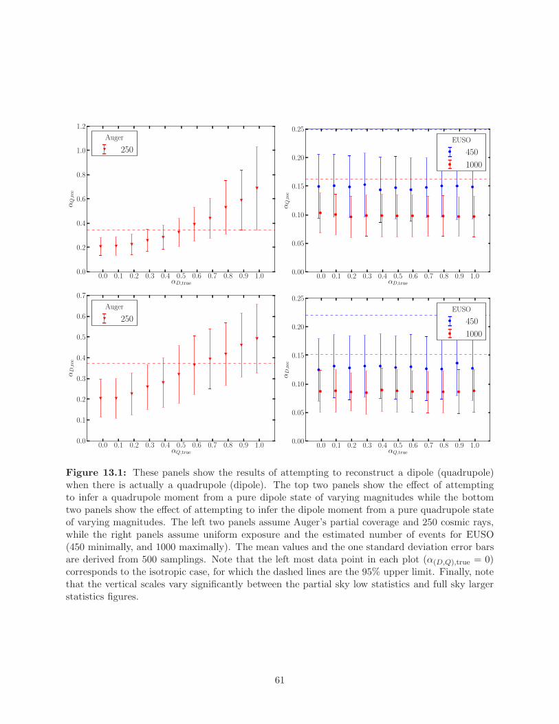
0.0 0.1 0.2 0.3 0.4 0.5 0.6 0.7 0.8 0.9 1.0αD,true
0.0
0.2
0.4
0.6
0.8
1.0
1.2
αQ,rec
Auger
250
0.0 0.1 0.2 0.3 0.4 0.5 0.6 0.7 0.8 0.9 1.0αD,true
0.00
0.05
0.10
0.15
0.20
0.25
αQ,rec
EUSO
450
1000
0.0 0.1 0.2 0.3 0.4 0.5 0.6 0.7 0.8 0.9 1.0αQ,true
0.0
0.1
0.2
0.3
0.4
0.5
0.6
0.7
αD,rec
Auger
250
0.0 0.1 0.2 0.3 0.4 0.5 0.6 0.7 0.8 0.9 1.0αQ,true
0.00
0.05
0.10
0.15
0.20
0.25
αD,rec
EUSO
450
1000
Figure 13.1: These panels show the results of attempting to reconstruct a dipole (quadrupole)when there is actually a quadrupole (dipole). The top two panels show the effect of attemptingto infer a quadrupole moment from a pure dipole state of varying magnitudes while the bottomtwo panels show the effect of attempting to infer the dipole moment from a pure quadrupole stateof varying magnitudes. The left two panels assume Auger’s partial coverage and 250 cosmic rays,while the right panels assume uniform exposure and the estimated number of events for EUSO(450 minimally, and 1000 maximally). The mean values and the one standard deviation error barsare derived from 500 samplings. Note that the left most data point in each plot (α(D,Q),true = 0)corresponds to the isotropic case, for which the dashed lines are the 95% upper limit. Finally, notethat the vertical scales vary significantly between the partial sky low statistics and full sky largerstatistics figures.
61

Chapter 14
Results
In this chapter we tally our results of the comparison of space based full sky and ground basedpartial sky experiments’ abilities to reconstruct anisotropies. The standard procedure involvessimulating a number of cosmic rays with a given dipolar or quadrupolar anisotropy shape andamplitude (αtrue) aligned in a random direction. We then reconstruct the amplitude (αrec) anddirection (here we assume knowledge of the kind of anisotropy – dipole or quadrupole – unlike inchapter 13) and compare to the true values. This process is repeated 500 times and the shownuncertainties are one standard deviation over the 500 repetitions.
14.1 Dipole results
In fig. 14.1 we compare the capabilities of design EUSO and Auger to reconstruct a dipole aniso-tropy. In this comparison, both advantages of EUSO, namely the increased FOV and the 4π skycoverage, are evident.
The first panel shows how changing only the exposure function between Auger and EUSO affectsthe value of the reconstructed dipole amplitude. For the same number of cosmic ray events, theEUSO reconstruction is a bit closer to the expected value and has a smaller variation than does theAuger reconstruction. In the next panel we show the angular separation between the actual dipoledirection and the reconstructed direction for Auger after a maximal amount of Auger data of ∼ 250cosmic ray events, compared to EUSO’s minimal and maximal data sizes: 450 and 1000 cosmic rayevents, respectively. Even for a pure dipole, Auger will only reach 10 accuracy in dipole directionfor a maximum strength dipole, αD = 1, while EUSO does much better. In the third panel wecompare both experiments at the same number of cosmic rays across a range of dipole strengths.Even if we assume that Auger will see significantly more cosmic rays than it is expected to, it stillhas a larger error in its ability to reconstruct a dipole of any amplitude than EUSO. The low dipolemagnitudes will always lead to a small erroneously reconstructed dipole due to random walkingaway from zero. Finally, in the fourth panel we show the discovery power of each experiment todistinguish a dipole amplitude from isotropy. We see that Auger with 250 events would claim adiscovery at five standard deviations above isotropy only if the dipole strength is 0.62 or greater– a situation that is unlikely given Auger’s anisotropy results to date [88]. EUSO could claim thesame significance if the dipole amplitude is 0.37, 0.30, 0.27, or greater, for 450, 750, or 1000 events,respectively. The EUSO significance should be enough to probe at high significance the weak signalcurrently reported by Auger.
14.2 Quadrupole results
In fig. 14.2 we again compare Auger and design EUSO in the context of quadrupole anisotropies.The same panels are plotted here as in fig. 14.1 except with an initial quadrupole rather than dipoleanisotropy, and a quadrupole reconstructed. We note that while the increased number of eventsthat EUSO will detect will certainly lead to a better resolution of the quadrupole amplitude (asshown in the first and fourth panels) and direction (as shown in the second panel), we see thatthe full sky coverage does not provide any benefit in this case (as deduced from the first and third
62

250 450 750 1000NCR
0.30
0.35
0.40
0.45
0.50
0.55
0.60
αD,rec
αD,true = 0.4
Auger
EUSO
0.1 0.2 0.3 0.4 0.5 0.6 0.7 0.8 0.9 1.0αD,true
0
10
20
30
40
50
60
70
∆θD(deg)
Auger, N = 250
EUSO, N = 450
EUSO, N = 1000
0.0 0.1 0.2 0.3 0.4 0.5 0.6 0.7 0.8 0.9 1.0αD,true
0.0
0.1
0.2
0.3
0.4
0.5
0.6
0.7
0.8
0.9
1.0
αD,rec
NCR = 450
Auger
EUSO
0.1 0.2 0.3 0.4 0.5 0.6 0.7 0.8 0.9 1.0αD,true
0
5
10
15
20
25
αD,true/∆
αD,rec
Auger, N = 250
EUSO, N = 450
EUSO, N = 750
EUSO, N = 1000
Figure 14.1: Reconstruction of the dipole amplitude and direction across various parameters.Each data point is the mean value (and one standard deviation error bar as applicable) determinedfrom 500 independent simulations. The dipole amplitude and direction for Auger’s partial coveragewere reconstructed with the K-matrix approach. The ordinate on the fourth panel, αtrue
∆αrec, labels
the number of standard deviations above αD = 0.
63
panels). This result numerically confirms the claims made in chapter 12 that Auger with c02 = 0does well with assumed quadrupole.
Even though EUSO gains no benefit from its full sky exposure for the determination of aquadrupole anisotropy, EUSO’s increased statistics will still lead to a detection sooner than Auger.Auger with 250 events would only be expected to claim a quadrupole discovery at five standarddeviations above isotropy if the quadrupole strength is 0.67 or greater. EUSO could claim the samesignificance if the quadrupole amplitude is 0.47, 0.36, 0.29, or greater, for 450, 750, or 1000 events,respectively.
64
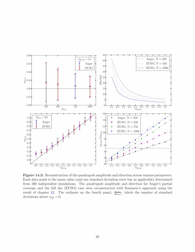
250 450 750 1000NCR
0.30
0.35
0.40
0.45
0.50
0.55
0.60
αQ,rec
αQ,true = 0.4
Auger
EUSO
0.1 0.2 0.3 0.4 0.5 0.6 0.7 0.8 0.9 1.0αQ,true
0
5
10
15
20
25
30
35
40
45
∆θQ(deg)
Auger, N = 250
EUSO, N = 450
EUSO, N = 1000
0.0 0.1 0.2 0.3 0.4 0.5 0.6 0.7 0.8 0.9 1.0αQ,true
0.0
0.1
0.2
0.3
0.4
0.5
0.6
0.7
0.8
0.9
1.0
αQ,rec
NCR = 450
Auger
EUSO
0.1 0.2 0.3 0.4 0.5 0.6 0.7 0.8 0.9 1.0αQ,true
0
2
4
6
8
10
12
14
16
αQ,true/∆
αQ,rec
Auger, N = 250
EUSO, N = 450
EUSO, N = 750
EUSO, N = 1000
Figure 14.2: Reconstruction of the quadrupole amplitude and direction across various parameters.Each data point is the mean value (and one standard deviation error bar as applicable) determinedfrom 500 independent simulations. The quadrupole amplitude and direction for Auger’s partialcoverage and the full sky (EUSO) case were reconstructed with Sommers’s approach using theresult of chapter 12. The ordinate on the fourth panel, αtrue
∆αrec, labels the number of standard
deviations above αQ = 0.
65
Chapter 15
Conclusions
The interesting result from chapter 12, bm2 ≈ am2 as given in eq. 12.19, occurs only in the case wherethe experimental latitude is near ±35. At these special latitudes, the reconstruction of a purequadrupole source distribution is not disadvantaged by partial sky coverage. By a lucky chance,Auger is located at precisely the correct latitude to benefit from the vanishing of c02. TA’s latitudeis sufficiently close to 35 to also benefit.
If Auger and TA reconstruct both a dipole and a quadrupole simultaneously, then the simpli-fication fails, since both experiments have significant dipole moments in their exposure functions.The confusion is apparent in the mixing within eqs. 12.12 and 12.13. With any source distributionthat contains more than a single nontrivial multipole, the partial sky coverage inherent in theseground based experiments exacts a significant price as shown in figs. 14.1 and 14.2.
Considering that an experiment 5 away from the optimal latitude reconstructs the quadrupolewell while 10 does not, we claim that experiments at latitudes 30 . |a0| . 40 can reconstruct apure quadrupole moment while ignoring their experiment’s particular exposure.
Many well motivated models predict, in the simplest limit, a dipolar or quadrupolar anisotropyin the UHECR flux. The importance of the two lowest nontrivial orders (ℓ = 1, 2) can be seen fromthe 2MRS distribution of the 5310 nearest galaxies that was demonstrated in fig. 10.1. Due to thelack of any conclusive anisotropy from the partial sky ground based experiments, we explored thepossible benefits that a full sky space based experiment, such as proposed EUSO, has over a groundbased experiment for detecting dipolar or quadrupolar anisotropies. In particular, we see that inaddition to the increased statistics that proposed EUSO brings over any ground based experiment,proposed EUSO significantly outperforms Auger when reconstructing a dipole. Moreover, for infer-ences of both the dipole and the quadrupole, partial sky experiments fail to differentiate betweenthe two due to the mixing of the spherical harmonics when truncated by the exposure function.This situation is not present with all sky observation, where the exposure function is nearly uniformand nonzero everywhere.
66
Appendix
B b10-cut
The source catalog from the 2MRS [12] has a ‘b10-cut’ applied to it. That is, only galaxies with|b| > 10 are included due to the obscuring effects of our own Milky Way galaxy. In order tocalculate the spherical harmonics correctly on a partial sky-map, this effect can be analyticallyconsidered due to the simple nature of the “exposure map” unlike that of Auger which has a highlynon-linear shape and misses much of the sky.
A uniform intensity distribution is given by
Iu(Ω) =1
4π. (B.1)
We then define another distribution over part of the sky by
Iu,<10(Ω) =1
4π
1 | cos θ| < cos(80)
0 else. (B.2)
where θ is the polar angle measured from the galactic north pole. Then the remaining sky lookslike
Iu,>10(Ω) = Iu(Ω)− Iu,<10(Ω) , (B.3)
Iu,>10(Ω) =1
4π
0 | cos θ| < cos(80)
1 else. (B.4)
Next we express the distribution of local galaxies by splitting the sky as expected,
Ig(Ω) = Ig,>10(Ω) + Ig,<10(Ω) . (B.5)
Since there is not complete information about Ig,<10, we replace it with a uniform distribution,
Ig(Ω) = Ig,>10(Ω) + Iu,<10(Ω) . (B.6)
We take the usual definition of amℓ from eq. 10.1,
I(Ω) =∞∑
ℓ=0
ℓ∑
m=−ℓ
amℓ Y mℓ (Ω) . (B.7)
By orthogonality of the Y mℓ ,
amℓ =
∫
Y mℓ (u)I(u)dΩ . (B.8)
By linearity, the coefficients are then,
(amℓ )g = (amℓ )g,>10 + (amℓ )u,<10 , (B.9)
where (amℓ )g,>10 is the quantity that will be measured and (amℓ )u,<10 is a correction to be appliedto give the desired quantity (amℓ )g. From eq. B.2 we note that Iu,<10(Ω) isn’t a function of φ anduse
∫
dφeimφ = 2πδm0 . (B.10)
67
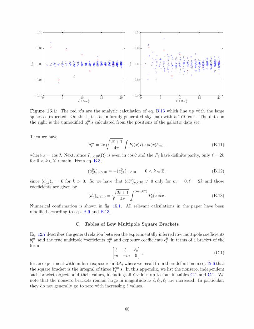
0 5 10 15 20
ℓ + 0.2m
ℓ
−0.10
−0.05
0.00
0.05
0.10aℓm
0 5 10 15 20
ℓ + 0.2m
ℓ
−0.10
−0.05
0.00
0.05
0.10
aℓm
Figure 15.1: The red x’s are the analytic calculation of eq. B.13 which line up with the largespikes as expected. On the left is a uniformly generated sky map with a ‘b10-cut’. The data onthe right is the unmodified amℓ ’s calculated from the positions of the galactic data set.
Then we have
amℓ = 2π
√
2ℓ+ 1
4π
∫
Pℓ(x)I(x)d(x)δm0 , (B.11)
where x = cos θ. Next, since Iu,<10(Ω) is even in cos θ and the Pℓ have definite parity, only ℓ = 2kfor 0 < k ∈ Z remain. From eq. B.3,
(a02k)u,>10 = −(a02k)u,<10 0 < k ∈ Z , (B.12)
since (a02k)u = 0 for k > 0. So we have that (amℓ )u,<10 6= 0 only for m = 0, ℓ = 2k and thosecoefficients are given by
(a0ℓ )u,<10 =
√
2ℓ+ 1
4π
∫ cos(80)
0Pℓ(x)dx . (B.13)
Numerical confirmation is shown in fig. 15.1. All relevant calculations in the paper have beenmodified according to eqs. B.9 and B.13.
C Tables of Low Multipole Square Brackets
Eq. 12.7 describes the general relation between the experimentally inferred raw multipole coefficientsbmℓ , and the true multipole coefficients amℓ and exposure coefficients c0ℓ , in terms of a bracket of theform
[
ℓ ℓ1 ℓ2m −m 0
]
, (C.1)
for an experiment with uniform exposure in RA, where we recall from their definition in eq. 12.6 thatthe square bracket is the integral of three Y m
ℓ ’s. In this appendix, we list the nonzero, independentsuch bracket objects and their values, including all ℓ values up to four in tables C.1 and C.2. Wenote that the nonzero brackets remain large in magnitude as ℓ, ℓ1, ℓ2 are increased. In particular,they do not generally go to zero with increasing ℓ values.
68
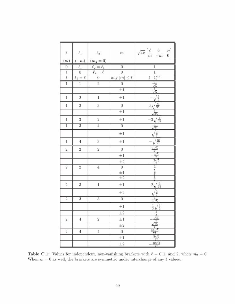
ℓ ℓ1 ℓ2 m√4π
[
ℓ ℓ1 ℓ2m −m 0
]
(m) (−m) (m2 = 0)
0 ℓ1 ℓ2 = ℓ1 0 1
ℓ 0 ℓ2 = ℓ 0 1
ℓ ℓ1 = ℓ 0 any |m| ≤ ℓ (−1)m
1 1 2 0 2√5
±1 1√5
1 2 1 ±1 −√
35
1 2 3 0 3√
335
±1 3√35
1 3 2 ±1 −3√
235
1 3 4 0 4√21
±1√
27
1 4 3 ±1 −√
1021
2 2 2 0 2√5
7
±1 −√57
±2 −2√5
7
2 2 4 0 67
±1 47
±2 17
2 3 1 ±1 −2√
635
±2√
37
2 3 3 0 43√5
±1 −13
√
25
±2 −23
2 4 2 ±1 −√307
±2√157
2 4 4 0 20√5
77
±1 −5√6
77
±2 −30√3
77
Table C.1: Values for independent, non-vanishing brackets with ℓ = 0, 1, and 2, when m2 = 0.When m = 0 as well, the brackets are symmetric under interchange of any ℓ values.
69
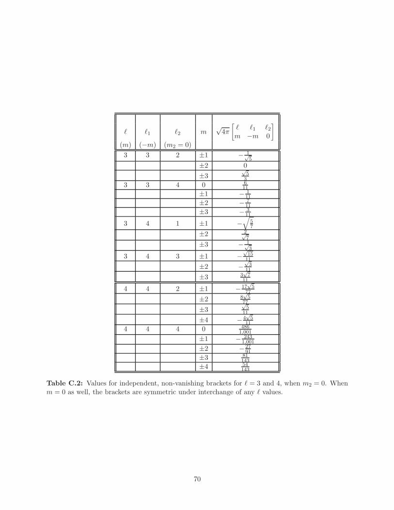
ℓ ℓ1 ℓ2 m√4π
[
ℓ ℓ1 ℓ2m −m 0
]
(m) (−m) (m2 = 0)
3 3 2 ±1 − 1√5
±2 0
±3√53
3 3 4 0 611
±1 − 111
±2 − 711
±3 − 311
3 4 1 ±1 −√
57
±2 2√7
±3 − 1√3
3 4 3 ±1 −√1511
±2 −√3
11
±3 3√7
11
4 4 2 ±1 −17√5
77
±2 8√5
77
±3√5
11
±4 −4√5
11
4 4 4 0 4861,001
±1 − 2431,001
±2 −2791
±3 81143
±4 54143
Table C.2: Values for independent, non-vanishing brackets for ℓ = 3 and 4, when m2 = 0. Whenm = 0 as well, the brackets are symmetric under interchange of any ℓ values.
70
Bibliography
[1] P. B. Denton and T. J. Weiler, “Using integral dispersion relations to extend the LHC reachfor new physics,” Phys. Rev. D 89 (Feb, 2014) 035013, arXiv:1311.1248 [hep-ph].
[2] JEM-EUSO Collaboration, P. B. Denton, L. A. Anchordoqui, A. A. Berlind, M. Richardson,and T. J. Weiler, “Sensitivity of orbiting JEM-EUSO to large-scale cosmic-ray anisotropies,”J. Phys. Conf. Ser. 531 (2014) 012004, arXiv:1401.5757 [astro-ph.IM].
[3] P. B. Denton and T. J. Weiler, “The Fortuitous Latitude of the Pierre Auger Observatoryand Telescope Array for Reconstructing the Quadrupole Moment,”Astrophys. J. 802 no. 1, (2015) 25, arXiv:1409.0883 [astro-ph.HE].
[4] P. B. Denton and T. J. Weiler, “Sensitivity of full-sky experiments to large scale cosmic rayanisotropies,” JHEAp 8 (2015) 1–9, arXiv:1505.03922 [astro-ph.HE].
[5] N. Arsene, L. I. Caramete, P. B. Denton, and O. Micu, “Quantum Black Holes Effects on theShape of Extensive Air Showers,” arXiv:1310.2205 [hep-ph].
[6] L. A. Anchordoqui, P. B. Denton, H. Goldberg, T. C. Paul, L. H. M. Da Silva, B. J. Vlcek,and T. J. Weiler, “Weinberg’s Higgs portal confronting recent LUX and LHC results togetherwith upper limits on B+ and K+ decay into invisibles,”Phys. Rev. D89 no. 8, (2014) 083513, arXiv:1312.2547 [hep-ph].
[7] P. B. Denton, H. Minakata, and S. J. Parke, “Compact Perturbative Expressions ForNeutrino Oscillations in Matter,” arXiv:1604.08167 [hep-ph].
[8] P. B. Denton, “Nu-Pert v0.2.2,” June, 2016. http://dx.doi.org/10.5281/zenodo.54629.https://github.com/PeterDenton/Nu-Pert.
[9] M. Block and F. Halzen, “Duality as a robust constraint on the LHC cross section,”Phys.Rev. D73 (2006) 054022, arXiv:hep-ph/0510238 [hep-ph].
[10] M. M. Block and F. Halzen, “Forward hadronic scattering at 8 TeV: predictions for theLHC,” Phys.Rev. D86 (2012) 014006, arXiv:1205.5514 [hep-ph].
[11] JEM-EUSO Collaboration, J. H. Adams et al., “An evaluation of the exposure in nadirobservation of the JEM-EUSO mission,” Astropart. Phys. 44 (2013) 76–90,arXiv:1305.2478 [astro-ph.HE].
[12] J. P. Huchra, L. M. Macri, K. L. Masters, T. H. Jarrett, P. Berlind, et al., “The 2MASSRedshift Survey - Description and Data Release,” Astrophys.J.Suppl. 199 (2012) 26,arXiv:1108.0669 [astro-ph.CO].
[13] H. Goldberg and T. J. Weiler, “Lower energy consequences of an anomalous high-energyneutrino cross section,” Phys. Rev. D 59 (Apr, 1999) 113005. http://link.aps.org/doi/10.1103/PhysRevD.59.113005.
[14] R. D. L. Kronig, “On the theory of dispersion of x-rays,”J. Opt. Soc. Am. 12 no. 6, (Jun, 1926) 547 – 556. Kronig includes the following footnote atthe beginning of his paper: “As Professor Kramers kindly informs me, he too has obtainedmost of the results derived in 3. (To be published shortly.)”.
71
[15] H. A. Kramers, “La diffusion de la lumiere par les atomes,” in Atti del CongressoInternazionale dei Fisici, Como-Pavia-Roma, vol. 2, pp. 545 – 557. 1927.
[16] M. Gell-Mann, M. L. Goldberger, and W. E. Thirring, “Use of causality conditions inquantum theory,” Phys. Rev. 95 (Sep, 1954) 1612 – 1627.
[17] P. Soding, “Real part of the proton-proton and proton-antiproton forward scatteringamplitude at high energies,” Physics Letters 8 no. 4, (1964) 285 – 287.
[18] M. Block and R. Cahn, “High-Energy pp and pp Forward Elastic Scattering and TotalCross-Sections,” Rev.Mod.Phys. 57 (1985) 563.
[19] CDF Collaboration, F. Abe et al., “Measurement of the pp total cross-section at√s = 546
GeV and 1800-GeV,” Phys. Rev. D50 (1994) 5550–5561.
[20] TOTEM Collaboration, G. Antchev et al., “Luminosity-independent measurements of total,elastic and inelastic cross-sections at
√s = 7 TeV,” Europhys. Lett. 101 (2013) 21004.
[21] R. M. Baltrusaitis, G. L. Cassiday, J. W. Elbert, P. R. Gerhardy, S. Ko, E. C. Loh,Y. Mizumoto, P. Sokolsky, and D. Steck, “Total Proton Proton Cross-Section at s**(1/2) =30-TeV,” Phys. Rev. Lett. 52 (1984) 1380–1383.
[22] M. Honda, M. Nagano, S. Tonwar, K. Kasahara, T. Hara, N. Hayashida, Y. Matsubara,M. Teshima, and S. Yoshida, “Inelastic cross-section for p-air collisions from air showerexperiment and total cross-section for p p collisions at SSC energy,”Phys. Rev. Lett. 70 (1993) 525–528.
[23] Pierre Auger Collaboration, P. Abreu et al., “Measurement of the proton-air cross-sectionat
√s = 57 TeV with the Pierre Auger Observatory,” Phys. Rev. Lett. 109 (2012) 062002,
arXiv:1208.1520 [hep-ex].
[24] R. J. Glauber, “Cross sections in deuterium at high energies,”Phys. Rev. 100 (Oct, 1955) 242–248.
[25] A. Alkin, J. Cudell, and E. Martynov, “Dispersion relations for meson-proton andproton-proton forward elastic scattering,” Few Body Syst. 53 (2012) 87 – 98,arXiv:1109.1306 [hep-ph].
[26] S. Mandelstam, “Determination of the pion - nucleon scattering amplitude from dispersionrelations and unitarity. General theory,” Phys.Rev. 112 (1958) 1344 – 1360.
[27] M. E. Peskin and D. V. Schroeder, An Introduction To Quantum Field Theory, pp. 230–236.Addison-Wesley Publishing Company, 1995. Two approaches are discussed. One based on anS-matrix approach and the other based on a Feynman diagram approach.
[28] M. Froissart, “Asymptotic behavior and subtractions in the mandelstam representation,”Phys. Rev. 123 (Aug, 1961) 1053–1057.
[29] Y. Azimov, “How Robust is the Froissart Bound?,” Phys.Rev. D84 (2011) 056012,arXiv:1104.5314 [hep-ph].
[30] A. Martin and S. Roy, “Froissart Bound on Total Cross-section without UnknownConstants,” Phys.Rev. D89 (2014) 045015, arXiv:1306.5210 [hep-ph].
72
[31] Y. I. Azimov, “Comment on “Froissart bound on total cross section without unknownconstants” by A. Martin and S.M. Roy [arXiv:1306.5210],” arXiv:1405.2448 [hep-ph].
[32] I. Y. Pomeranchuk, “Equality of total cross sections of interactions of nucleons andantinucleons at high energies,” JETP 34 (1958) 725.
[33] R. J. Eden, “Use of unitarity in proving pomeranchuk’s theorem on cross sections at highenergies,” Phys. Rev. Lett. 16 (Jan, 1966) 39–41.
[34] T. Kinoshita in Perspectives in Modern Physics, R. E. Marshak, ed., p. 211. John Wiley andSons, 1st ed., 1966.
[35] Particle Data Group Collaboration, J. Beringer et al., “Review of particle physics,”Phys. Rev. D 86 (Jul, 2012) 010001.
[36] M. Block and F. Halzen, “Evidence for the saturation of the Froissart bound,”Phys.Rev. D70 (2004) 091901, arXiv:hep-ph/0405174 [hep-ph].
[37] M. M. Block and F. Halzen, “New experimental evidence that the proton developsasymptotically into a black disk,” Phys.Rev. D86 (2012) 051504,arXiv:1208.4086 [hep-ph].
[38] totem-experiment.web.cern.ch/totem-experiment.
[39] G. Antchev, P. Aspell, I. Atanassov, V. Avati, J. Baechler, et al., “First measurement of thetotal proton-proton cross section at the LHC energy of
√s =7 TeV,”
Europhys.Lett. 96 (2011) 21002, arXiv:1110.1395 [hep-ex].
[40] “Luminosity determination using the atlas detector,” Tech. Rep. ATLAS-CONF-2010-060,CERN, Geneva, Jul, 2010.
[41] home.web.cern.ch/about/experiments/lhcf.
[42] ATLAS Collaboration Collaboration, G. Aad et al., “Luminosity Determination in ppCollisions at sqrt(s)=7 TeV Using the ATLAS Detector at the LHC,”Eur.Phys.J. C71 (2011) 1630, arXiv:1101.2185 [hep-ex].
[43] J. Kaspar, “Totem results on elastic scattering and total cross-section,” in EDS Blois 2013.2013. http://indico.cern.ch/event/267509/contributions/1605297/attachments/478067/661405/jan_kaspar_eds_2013.pdf.
[44] H.-T. Wei, R.-Y. Zhang, L. Guo, L. Han, W.-G. Ma, et al., “Probe R-parity violating stopresonance at the LHeC,” JHEP 1107 (2011) 003, arXiv:1107.4461 [hep-ph].
[45] F. Bazzocchi, S. Morisi, E. Peinado, J. W. F. Valle, and A. Vicente, “Bilinear R-parityviolation with flavor symmetry,” JHEP 01 (2013) 033, arXiv:1202.1529 [hep-ph].
[46] B. Bhattacherjee, J. L. Evans, M. Ibe, S. Matsumoto, and T. T. Yanagida, “Naturalsupersymmetrys last hope: R-parity violation via UDD operators,”Phys. Rev. D87 no. 11, (2013) 115002, arXiv:1301.2336 [hep-ph].
[47] CMS Collaboration, S. Chatrchyan et al., “Search for top squarks in R-parity-violatingsupersymmetry using three or more leptons and b-tagged jets,”Phys. Rev. Lett. 111 no. 22, (2013) 221801, arXiv:1306.6643 [hep-ex].
73

[48] CMS Collaboration, A. Cakir, “Search for R-Parity Violating Supersymmetry at the CMSExperiment,” PoS EPS-HEP2013 (2013) 264, arXiv:1310.3598 [hep-ph].
[49] D. Chialva, R. Iengo, and J. G. Russo, “Cross sections for production of closed superstringsat high energy colliders in brane world models,” Phys.Rev. D71 (2005) 106009,arXiv:hep-ph/0503125 [hep-ph].
[50] T. Kaluza, “On the Problem of Unity in Physics,” Sitzungsber. Preuss. Akad. Wiss. Berlin(Math. Phys.) 1921 (1921) 966–972.
[51] O. Klein, “Quantum Theory and Five-Dimensional Theory of Relativity. (In German andEnglish),” Z. Phys. 37 (1926) 895–906. [Surveys High Energ. Phys.5,241(1986)].
[52] J. Gao, M. Guzzi, J. Huston, H.-L. Lai, Z. Li, P. Nadolsky, J. Pumplin, D. Stump, and C. P.Yuan, “CT10 next-to-next-to-leading order global analysis of QCD,”Phys. Rev. D89 no. 3, (2014) 033009, arXiv:1302.6246 [hep-ph].
[53] ATLAS Collaboration Collaboration, G. Aad et al., “Measurement of the InelasticProton-Proton Cross-Section at
√s = 7 TeV with the ATLAS Detector,”
Nature Commun. 2 (2011) 463, arXiv:1104.0326 [hep-ex].
[54] A. Martin and T. Spearman, Elementary Particle Theory. North-Holland, 1970.
[55] TOTEM Collaboration, J. Kapar, “TOTEM Results on Elastic Scattering and TotalCross-Section,” in Proceedings, 15th conference on Elastic and Diffractive scattering (EDSBlois 2013). 2013. arXiv:1310.3178 [physics.ins-det].
[56] P. Auger, P. Ehrenfest, R. Maze, J. Daudin, and A. F. Robley, “Extensive cosmic rayshowers,” Rev. Mod. Phys. 11 (1939) 288–291.
[57] Pierre Auger Collaboration, A. Aab et al., “Depth of maximum of air-shower profiles atthe Pierre Auger Observatory. I. Measurements at energies above 1017.8eV,”Phys. Rev. D90 no. 12, (2014) 122005, arXiv:1409.4809 [astro-ph.HE].
[58] R. U. Abbasi et al., “Study of Ultra-High Energy Cosmic Ray composition using TelescopeArrays Middle Drum detector and surface array in hybrid mode,”Astropart. Phys. 64 (2015) 49–62, arXiv:1408.1726 [astro-ph.HE].
[59] M. S. Pshirkov, P. G. Tinyakov, P. P. Kronberg, and K. J. Newton-McGee, “Deriving globalstructure of the Galactic Magnetic Field from Faraday Rotation Measures of extragalacticsources,” Astrophys. J. 738 (2011) 192, arXiv:1103.0814 [astro-ph.GA].
[60] R. Jansson and G. R. Farrar, “A New Model of the Galactic Magnetic Field,”Astrophys. J. 757 (2012) 14, arXiv:1204.3662 [astro-ph.GA].
[61] T. Kahniashvili, A. G. Tevzadze, S. K. Sethi, K. Pandey, and B. Ratra, “Primordialmagnetic field limits from cosmological data,” Phys. Rev. D82 (2010) 083005,arXiv:1009.2094 [astro-ph.CO].
[62] J. E. Gunn and J. P. Ostriker, “Acceleration of high-energy cosmic rays by pulsars,”Phys. Rev. Lett. 22 (1969) 728–731.
74
[63] J. Pruet, S. Guiles, and G. M. Fuller, “Light element synthesis in high entropy relativisticflows associated with gamma-ray bursts,” Astrophys. J. 580 (2002) 368–373,arXiv:astro-ph/0205056 [astro-ph].
[64] M. Lemoine, “Nucleosynthesis in gamma-ray bursts outflows,”Astron. Astrophys. 390 (2002) L31, arXiv:astro-ph/0205093 [astro-ph].
[65] B. Groves, T. Heckman, and G. Kauffmann, “Emission-line Diagnostics of Low MetallicityAGN,” Mon. Not. Roy. Astron. Soc. 371 (2006) 1559–1569,arXiv:astro-ph/0607311 [astro-ph].
[66] S. Mathur and D. Fields, “Metallicity measurements in AGNs,”AIP Conf. Proc. 1135 (2009) 209–214, arXiv:0901.1323 [astro-ph.GA].
[67] K. Fang, K. Kotera, and A. V. Olinto, “Newly-born pulsars as sources of ultrahigh energycosmic rays,” Astrophys. J. 750 (2012) 118, arXiv:1201.5197 [astro-ph.HE].
[68] Pierre Auger Collaboration, J. Abraham et al., “Correlation of the highest-energy cosmicrays with the positions of nearby active galactic nuclei,” Astropart. Phys. 29 (2008) 188–204,arXiv:0712.2843 [astro-ph]. [Erratum: Astropart. Phys.30,45(2008)].
[69] Pierre Auger Collaboration, A. Aab et al., “Searches for Anisotropies in the ArrivalDirections of the Highest Energy Cosmic Rays Detected by the Pierre Auger Observatory,”Astrophys. J. 804 no. 1, (2015) 15, arXiv:1411.6111 [astro-ph.HE].
[70] Telescope Array Collaboration, R. U. Abbasi et al., “Indications of Intermediate-ScaleAnisotropy of Cosmic Rays with Energy Greater Than 57 EeV in the Northern SkyMeasured with the Surface Detector of the Telescope Array Experiment,”Astrophys. J. 790 (2014) L21, arXiv:1404.5890 [astro-ph.HE].
[71] M. M. Winn, J. Ulrichs, L. S. Peak, C. B. A. McCusker, and L. Horton, “The cosmic-rayenergy spectrum above 10 17 ev,” Journal of Physics G: Nuclear Physics 12 no. 7, (1986)653. http://stacks.iop.org/0305-4616/12/i=7/a=015.
[72] AGASA Collaboration, H. Ohoka, S. Yoshida, M. Takeda, et al., “Further development ofdata acquisition system of AGASA,” Nucl.Instrum.Meth. A385 (1997) 268–276.
[73] L. A. Anchordoqui, C. Hojvat, T. P. McCauley, T. C. Paul, S. Reucroft, et al., “Full - skysearch for ultrahigh-energy cosmic ray anisotropies,” Phys.Rev. D68 (2003) 083004,arXiv:astro-ph/0305158 [astro-ph].
[74] Pierre Auger Collaboration Collaboration, P. Abreu et al., “Search for First HarmonicModulation in the Right Ascension Distribution of Cosmic Rays Detected at the PierreAuger Observatory,” Astropart.Phys. 34 (2011) 627–639, arXiv:1103.2721 [astro-ph.HE].
[75] Pierre Auger Collaboration Collaboration, P. Abreu et al., “Large scale distribution ofarrival directions of cosmic rays detected above 1018 eV at the Pierre Auger Observatory,”Astrophys.J.Suppl. 203 (2012) 34, arXiv:1210.3736 [astro-ph.HE].
[76] L. A. Anchordoqui, H. Goldberg, and T. J. Weiler, “Update on tests of the Cen Aneutron-emission model of highest energy cosmic rays,” Phys.Rev. D84 (2011) 067301,arXiv:1103.0536 [astro-ph.HE].
75
[77] Pierre Auger Collaboration Collaboration, P. Abreu et al., “Constraints on the origin ofcosmic rays above 1018 eV from large scale anisotropy searches in data of the Pierre AugerObservatory,” Astrophys.J. 762 (2012) L13, arXiv:1212.3083 [astro-ph.HE].
[78] Pierre Auger Collaboration, A. Aab et al., “Large Scale Distribution of Ultra High EnergyCosmic Rays Detected at the Pierre Auger Observatory With Zenith Angles up to 80,”Astrophys.J. 802 no. 2, (2015) 111, arXiv:1411.6953 [astro-ph.HE].
[79] L. Anchordoqui, T. C. Paul, S. Reucroft, and J. Swain, “Ultrahigh-energy cosmic rays: TheState of the art before the Auger Observatory,” Int. J. Mod. Phys. A18 (2003) 2229–2366,arXiv:hep-ph/0206072 [hep-ph].
[80] Pierre Auger Collaboration, I. Allekotte et al., “The Surface Detector System of the PierreAuger Observatory,” Nucl. Instrum. Meth. A586 (2008) 409–420,arXiv:0712.2832 [astro-ph].
[81] Pierre Auger Collaboration, J. Abraham et al., “The Fluorescence Detector of the PierreAuger Observatory,” Nucl. Instrum. Meth. A620 (2010) 227–251,arXiv:0907.4282 [astro-ph.IM].
[82] K. Greisen, “End to the cosmic ray spectrum?,” Phys. Rev. Lett. 16 (1966) 748–750.
[83] G. T. Zatsepin and V. A. Kuzmin, “Upper limit of the spectrum of cosmic rays,” JETP Lett.4 (1966) 78–80. [Pisma Zh. Eksp. Teor. Fiz.4,114(1966)].
[84] Pierre Auger Collaboration, J. Abraham et al., “Observation of the suppression of the fluxof cosmic rays above 4× 10¹⁹eV,” Phys. Rev. Lett. 101 (2008) 061101,arXiv:0806.4302 [astro-ph].
[85] H. Tokuno et al., “New air fluorescence detectors employed in the Telescope Arrayexperiment,” Nucl. Instrum. Meth. A676 (2012) 54–65, arXiv:1201.0002 [astro-ph.IM].
[86] Telescope Array Collaboration, T. Abu-Zayyad et al., “The surface detector array of theTelescope Array experiment,” Nucl. Instrum. Meth. A689 (2013) 87–97,arXiv:1201.4964 [astro-ph.IM].
[87] P. Sommers, “Cosmic ray anisotropy analysis with a full-sky observatory,”Astropart.Phys. 14 (2001) 271–286, arXiv:astro-ph/0004016 [astro-ph].
[88] Pierre Auger Collaboration Collaboration, O. Deligny, “Large-Scale Distribution ofArrival Directions of Cosmic Rays Detected at the Pierre Auger Observatory Above 10 PeV,”J.Phys.Conf.Ser. 531 (2014) 012002, arXiv:1403.6314 [astro-ph.HE].
[89] G. B. Thomson, “Results from the Telescope Array Experiment,” PoS ICHEP2010 (2010)448, arXiv:1010.5528 [astro-ph.HE].
[90] JEM-EUSO Collaboration, J. H. Adams, Jr. et al., “The JEM-EUSO Mission:Contributions to the ICRC 2013,” 2013. arXiv:1307.7071 [astro-ph.IM].
[91] OWL Collaboration, J. F. Krizmanic, J. W. Mitchell, and R. E. Streitmatter, “Optimizationof the Orbiting Wide-angle Light Collectors (OWL) Mission for Charged-Particle andNeutrino Astronomy,” in Proceedings, 33rd International Cosmic Ray Conference(ICRC2013): Rio de Janeiro, Brazil, July 2-9, 2013, p. 1085. 2013.arXiv:1307.3907 [astro-ph.IM].
76
[92] Pierre Auger Collaboration, A. Aab et al., “The Pierre Auger Observatory: Contributionsto the 33rd International Cosmic Ray Conference (ICRC 2013),” in Proceedings, 33rdInternational Cosmic Ray Conference (ICRC2013). 2013.arXiv:1307.5059 [astro-ph.HE]. http://lss.fnal.gov/archive/2013/conf/fermilab-conf-13-285-ad-ae-cd-td.pdf.
[93] See the figures at http://en.wikipedia.org/wiki/Spherical_harmonics for usefulvisualizations.
[94] See e.g. Arfken, G.B. and Weber, H.J., Mathematical Methods for Physicists. AcademicPress, 6th ed., 2005.
[95] O. E. Kalashev, B. Khrenov, P. Klimov, S. Sharakin, and S. V. Troitsky, “Global anisotropyof arrival directions of ultrahigh-energy cosmic rays: capabilities of space-based detectors,”JCAP 0803 (2008) 003, arXiv:0710.1382 [astro-ph].
[96] S. Mollerach and E. Roulet, “A New method to search for a cosmic ray dipole anisotropy,”JCAP 0508 (2005) 004, arXiv:astro-ph/0504630 [astro-ph].
[97] P. Billoir and O. Deligny, “Estimates of multipolar coefficients to search for cosmic rayanisotropies with non-uniform or partial sky coverage,” JCAP 0802 (2008) 009,arXiv:0710.2290 [astro-ph].
[98] J. Aublin and E. Parizot, “Generalized 3D-reconstruction method of a dipole anisotropy incosmic-ray distributions,” Astron. Astrophys. 441 (2005) 407,arXiv:astro-ph/0504575 [astro-ph].
[99] J. Linsley, “Fluctuation effects on directional data,” Phys. Rev. Lett. 34 (1975) 1530–1533.
77