methods for applied macroeconomics research - ch1

7/30/2019 methods for applied macroeconomics research - ch1

http://slidepdf.com/reader/full/methods-for-applied-macroeconomics-research-ch1 1/28

Chapter 1: Preliminaries

This chapter reviews background concepts and a few results used at some stage or anotherin the rest of the book. The material we present is dispersed in a variety of advancedprobability, stochastic process and time series textbooks. Here we only summarize conceptsand results which are useful from the point of view we take in this book, i.e. how to confrontdynamic stochastic general equilibrium (DSGE) models to the data.

The chapter is divided in six sections. The first defines what a stochastic process is.The second examines the asymptotic behavior of stochastic processes by introducing fourconcepts of convergence; characterizes the relationships among various definitions and high-lights diff erences. Section 3 introduces time series concepts which are of use in the nextchapters. Since the majority of econometric estimators are continuous functions of stochas-tic processes, we also present a few results concerning the properties of such functions.Section 4 deals with laws of large numbers. Such laws are useful to insure that functions of stochastic processes converge to appropriate limits. We examine three situations often en-countered in practice: a case where observations are dependent and identically distributed;one where they are dependent and heterogeneously distributed and one where they are mar-

tingale diff erences. AS we will see, relaxation of the homogeneity condition comes togetherwith stronger restrictions on the moment structure of the process. Section 5 describes threecentral limit theorems corresponding to the three situations analyzed in section 4. Centrallimit theorems are useful to derive the distribution of functions of stochastic processes andare the basis for (classical) tests of hypotheses and for some model evaluation criteria.

Section 6 presents elements of spectral analysis. Spectral analysis is useful for breakingdown economic time series into components (trends, cycles, etc.), for building measuresof persistence of shocks, for analyzing formulas for the asymptotic covariance matrix of certain estimators and for defining measures of distance between models and the data. Itmay be challenging at first. However, once it is realized that most of the functions typicallyperformed by modern electronics use spectral methods (frequency modulation in a stereo;

frequency band reception in a cellular phone, etc.), the reader should feel more comfortablewith it. Spectral analysis off ers an alternative way to look at time series translating seriallydependent time observations in contemporaneously independent frequency observations.This change of coordinates allows us to analyze the primitive cycles which compose timeseries, discuss their length, their amplitude and their persistence.

Whenever not explicitly stated, everything presented in this chapter applies to both

1



2

scalar and vector stochastic processes. The notation {yt(κ )}∞t=−∞ indicates the sequence{. . . , y0(κ ),y1(κ ), . . . , yt(κ ), . . .} where for each j, the random variable y j(κ ) is a function of the state

of nature κ ∈ K, i.e. y j : K → R, where R is the real line and K the space of states of nature. To simplify the notation at times we simply write {yt(κ )} or yt. A normal randomvariable with zero mean and variance Σy is denoted by yt ∼ N(0,Σy) and a random variableuniformly distributed over the interval [a1, a2] is denoted by yt ∼ U[a1, a2]. Finally, iidindicates identically and independently distributed random variables.

1.1 Stochastic Processes

D efinition 1.1 (Stochastic Process 1): A stochastic process {yt(κ )}∞t=1 is a sequence of random vectors together with mutually consistent joint probability distributions for fi nite

subsequences {yt(κ

)}

ti

t=t1, e.g. , {yt1 . . . yti} ∼N

(0,Σy) for all i and for

fi xed

κ

.

D efinition 1.2 (Stochastic Process 2): A stochastic process {yt(κ )}∞t=1 is a probability measure de fi ned on sets of sequences of real vectors (the “paths” of the process).

Definition 1.1 is incomplete in the sense that it does not specify what a consistent joint prob-

ability distribution is. For example, unless all variables are independent,P (yt1 ,...,yti0 )

P (yt1 ,...,yti0|yt1 ,...,yti)

6= P (yt1 . . . yti) for i0 > i. Since in macro-time series frameworks the case of independentlydistributed yt is rare, such a definition is impractical. The second definition implies, amongother things, that the set of paths X = {y : yt(κ ) ≤ %} for arbitrary % ∈ R, t fixed,has well-defined probabilities. In other words, choosing diff erent % ∈ R for a given t,

and performing countable unions, finite intersections and complementing the above set of paths, we generate a set of events with proper probabilities. Note also that the yt path isunrestricted for all τ ≤ t: the realization needs to be below % only at t. In what follows,we will use definition 1.2 and the notation yt(κ ) indicates that the random variable yt is afunction of both time t and the event κ ∈ K. Observable time series will be realizations of a stochastic process {yt(κ )}∞t=1 given κ .

Example 1.1 Three examples of simple stochastic processes are the following:1) yt = e1 cos(t × e2) where e1, e2 are random variables, e1 > 0 and e2 ∼ U[0, 2π). Here ytis periodic: e1 controls the amplitude and e2 the periodicity of yt.2) yt is such that P [yt = ±1] = 0.5 for all t. Such a process has no memory and fl ips

between -1 and 1 at each t.3) yt = PT t=1 et, et iid ∼ (0, 1). Then yt is a random walk with no drift.

Example 1.2 It is easy to generate complex stochastic processes from primitive ones. For example, if e1t ∼ N(0,1) and e2t ∼ U(0, 1] and they are independent of each other, yt =e2t exp{ e1t

1+e1t} is a stochastic process. What are the mean and the variance of yt?



Methods for Applied Macro Research 1: Preliminaries 3

1.2 Concepts of Convergence

1.2.1 Almost sure (a.s.) convergence

The concept of a.s. convergence is an extension of the concept of convergence employed forsequences of real numbers. In real analysis we have the following definition:

Definition 1.3 Let {y1, . . . , y j} be a sequence of real numbers. It converges to y if lim j→∞ y j = y.

Example 1.3 To illustrate de fi nition 1.3, let y j = 1 − 1 j . Then limn→∞ y j = 1. On the

other hand, if y j = (−1) j, lim j→∞ y j is undetermined. Finally, if y j = y j, lim j→∞ y j exists if y ≤ 1.

When we deal with stochastic processes, the object of interest are functions of the stateof nature. However, once κ is drawn, the sequence {y

1(κ ), . . . , y

t(κ )} looks like a sequence

of non-random numbers. Hence, given κ , we can use a concept of convergence similar tothe one used for real numbers.

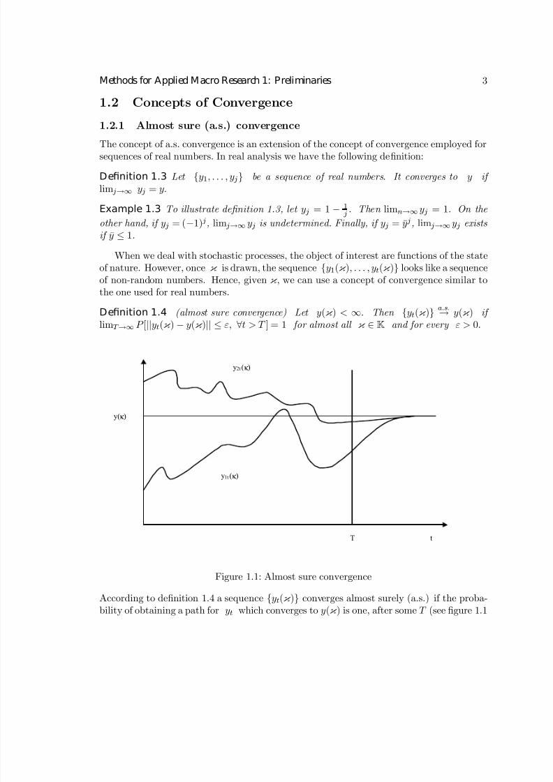
Definition 1.4 (almost sure convergence) Let y(κ ) < ∞. Then {yt(κ )}a.s.→ y(κ ) if

limT →∞ P [||yt(κ ) − y(κ )|| ≤ ε, ∀t > T ] = 1 for almost all κ ∈ K and for every ε > 0.

T t

y(κ )

y1t (κ )

y2t(κ )

Figure 1.1: Almost sure convergence

According to definition 1.4 a sequence {yt(κ )} converges almost surely (a.s.) if the proba-bility of obtaining a path for yt which converges to y(κ ) is one, after some T (see figure 1.1



4

for two such paths). The probability here is taken over κ ’s. Note that the definition impliesthat failure to converge is possible, but it happens on a null set (over which yt(κ ) → ±∞),which has zero Lebesgue measure. When K is infinite dimensional, a.s. convergence is

called convergence almost everywhere; sometimes a.s. convergence is termed convergencewith probability 1 (w.p.1) or strong consistency criteria.

Since in most applications we will be interested in continuous functions of stochasticprocesses, we describe the limiting behavior of functions of a.s. convergent sequences.

P ropositi on 1.1 Let {yt(κ )} be such that {yt(κ )}a.s.→ y(κ ). Let h be a n × 1 vector of

functions, continuous at y(κ ). Then h(yt(κ ))a.s.→ h(y(κ )). 2

Proposition 1.1 is a simple extension of the standard result that continuous functions of convergent sequences are convergent. In fact, for fixed κ , if {yt(κ )} → y(κ ) then h(yt(κ )) →h(y(κ )). Since the set [κ : yt(κ ) → y(κ )] ⊂ [κ : h(yt(κ )) → h(y(κ ))] and since 1 =

limT →∞P [||yt(κ

) − y(κ

)|| ≤ ², ∀t > T ] ≤ limT →∞P [||h(yt(κ

)) − h(yt(κ

))|| < ², ∀t > T ] ≤1, h(yt(κ ))

a.s.→ h(y(κ )).

Example 1.4 Let {yt(κ )} = 1 − 1t for a given κ and let h(yt(κ )) = 1

T

Pt yt(κ ). Then

h(yt(κ )) is continuous at limt→∞ yt(κ ) = 1 and h(yt(κ ))a.s.→ 1.

Exercise 1.1 Suppose {yt(κ )} = 1/t with probability 1− 1/t and {yt(κ )} = t with proba-bility t. Does {yt(κ )} converge almost surely to 1?

In some applications we will be interested in examining cases where a.s. convergence doesnot hold. This can be the case when the observations have a probability density functionthat changes over time or when matrices appearing in the expression for estimators do not

converge to fixed limits. In these cases even though h(y1t(κ )) does not converge toh(y(κ )), it may be the case that the distance between h(y1t(κ )) and h(y2t(κ )) becomesarbitrarily small as t → ∞ where {y2t(κ )} is another sequence of random variables. Toexamine this type of convergence we need the following definition.

D efinition 1.5 (Uniform Continuity): h is uniformly continuous on R1 ⊂ Rm if for ∀² > 0 there exists a ∆(²) > 0 such that if {y1t(κ )}, {y2t(κ )} ∈ R1 and |y1t,i(κ ) −y2t,i(κ )| < ∆(²), i = 1, . . . , m , then |h j(y1t(κ )) − h j(y2t(κ ))| < ², j = 1, . . . , n .

The concept of uniform continuity is graphically illustrated in figure 1.2 for m = n = 1.

Exercise 1.2 Show that uniform continuity implies continuity but not vice versa. Show that if R1 is compact, continuity implies uniform continuity.

Example 1.5 Functions which are continuous but not uniformly continuous are easy toconstruct. Let R1 = (0, 1) and let h(yt(κ )) = 1

yt. Clearly h is continuous over R1. However,

it is not uniformly continuous. To show this it is enough to show that for all ² > 0, ∆ > 0




y2

y1

∆ (ε )

ℜ 1

h( y2 )

h( y1 )

ε

Figure 1.2: Uniform Continuity

we can fi nd sequences y1t(κ ) and y2t(κ ) ∈ R1 for which |y1t−y2t| < ² and |h(y1t)−h(y2t)| >∆(²). For example, set y2t = 0.5y1t. Then conditions reduce to |y1t2 | < ² and | 1

y1t| > ∆(²)

which are satis fi ed for 0 < |y1t| < min{ 1∆(²) , 2², 1}.

What is missing in the example 1.5 and instead is present in the next proposition is thecondition that h is a defined on a compact set.

P ropositi on 1.2 Let h be continuous on a compact set R2 ∈ Rm. Suppose {y1t(κ )} and {y2t(κ )} are such that {y1t(κ )} − {y2t(κ )}

a.s.→ 0 and there exists an ² > 0 such that for all t > T , y2t is interior to R2, uniformly in t; that is, the set [|y1t − y2t| < ²] ⊂ R2, tlarge. Then h(y1t(κ ))

−h(y2t(κ ))

a.s.

→0. 2

The logic of proposition 1.2 is simple. Since R2 is compact, h j , j = 1, . . . , n is uniformlycontinuous on R2. Choose κ such that {y1t(κ )} − {y2t(κ )} → 0, t → ∞. Since y2t(κ ) isin the interior of R2, for all R2 sufficiently large, uniformly in t, and since {y1t(κ )} −{y2t(κ )} → 0, y1t is in the interior of R, for t large. By uniform continuity, for any² > 0, there exists a ∆(²) > 0 such that if |y1t,i(κ ) − y2t,i| < ∆(²) i = 1, . . . m , then|h j(y1t(κ )) − h j(y2t(κ ))| < ². Since |y1t,i(κ ) − y2t,i| < ∆(²), for all t sufficiently large and

almost every κ , |h j(y1t(κ )) − h j(y2t(κ ))|a.s.→ 0 for every j = 1, . . . n .

One application of proposition 1.2 is the following: suppose {y1t(κ )} is some actual timeseries and {y2t(κ )} is its simulated counterpart obtained from a model, fixing the parametersand given κ , and h be some continuous statistics, e.g. the mean or the variance. Then the

proposition tells us that if simulated and actual paths are close enough as t → ∞, then thecorresponding statistics generated from these paths will also be close as t → ∞.

1.2.2 Convergence in Probability

Convergence in probability is weaker than convergence almost sure, as it is shown next.



6

D efinition 1.6 (Convergence in Probability) If there exists a y(κ ) < ∞ such that, for

every ² > 0, P [κ : ||yt(κ ) − y(κ )|| > ²] → 0, for t → ∞, then {yt(κ )}P → y.

Definition 1.6 can be restated using the concept of boundness in probability.

D efinition 1.7 yt is bounded in probability denoted by O p(1)), if for any arbitrary ∆1 > 0there exists a ∆2 such that P [κ : ||yt(κ ) − y(κ )|| > ∆2] < ∆1. If ∆2 → 0 as t → ∞,{yt(κ )} converges in probability to y(κ ).

Exercise 1.3 Use the de fi nitions to show that almost sure convergence implies convergence in probability.

P → is weaker thana.s.→ because in the former we only need the joint distribution of (yt, y)

not the joint distribution of (yt, y

τ , y)

∀τ > T.

P

→implies that it is less likely that one

element of the {yt(κ )} sequence is more than an ² away from y as t → ∞. a.s.→ impliesthat after T, the path of {yt(κ )} is not far from y as T → ∞. Hence, it is easy to build

examples whereP → does not imply

a.s.→ .

Example 1.6 Let yt and yτ be independent ∀t, τ , let yt be either 0 or 1 and let

P [yt = 0] =

1/2 t = 1, 22/3 t = 3, 43/4 t = 5 · · · 84/5 t = 9 · · ·16

Then P [yt = 0] = 1 − 1 j for t = 2( j−1)+1, . . . , 2 j so that yt

P → 0. This is because the probability that yt is in one of these classes is 1/j and, as t → ∞, the number of classes goes to in fi nity. However, yt does not converge almost surely to zero since the probability that a convergent path is drawn is zero; i.e., if at t we draw yt = 1, there is a non-negligible

probability that yt+1 = 1 is drawn. Hence, ytP → 0 is too slow to insure that yt

a.s.→ 0.

Although convergence in probability does not imply almost sure convergence, the fol-lowing result is useful:

R esult 1.1 If yt(κ )P

→yt, there exist a subsequence ytj (κ ) such that ytj(κ )

a.s.

→y(t)

(see, e.g., Lukacs, 1975, p. 48).

Since convergence in probability allows a more erratic behavior in the converging sequencethan almost sure convergence, one can obtain almost sure convergence by disregarding theerratic elements of the sequence. The concept of convergence in probability is useful toshow “weak” consistency of certain estimators.




Example 1.7 (i) Let yt be a sequence of iid random variables with E (yt) < ∞. Then 1T

PT t=1 yt

a.s.→ E (yt) (Kolmogorov strong law of large numbers).

(ii) Let yt be a sequence of uncorrelated random variables, E (yt) < ∞, var(yt) = σ2y <

∞, cov(yt, yt−τ ) = 0 for all τ 6= 0. Then 1T

PT t=1 yt

P → E (yt) (Chebyshev weak law of large numbers).

As example 1.7 indicates strong consistency requires iid random variables, while for weakconsistency we just need a set of uncorrelated random variables with identical means andvariances. Note also that, weak consistency requires restrictions on the second moments of the sequence restrictions which are not needed in the first case.

The analogs of propositions 1.1 and 1.2 for convergence in probability can be easilyobtained.

P ropositi on 1.3 Let {yt(κ )} be such that yt(κ ) P → y(κ ). Then h(yt(κ )) P → h(y(κ )), for any h which is continuous at y(κ ) (for a proof, see White, 1984, p. 23). 2

P ropositi on 1.4 Let h be continuous on a compact R1 ⊂ Rm. Let {y1t(κ )} and {y2t(κ )}

be such that y1t(κ ) − y2t(κ )P → 0 for t → ∞. Then h(y1t(κ )) − h(y2t(κ ))

P −→ 0 (for a proof, see White, 1984, p. 25). 2

In some time-series applications the stochastic process yt may converge to a limit whichis not in the space of the random variables which make up the sequence; e.g., the sequencedefined by yt =

P j e j where each e j is stationary has a limit which is not in the space of

stationary variables. In other cases, the limit point y(κ ) may be unknown. In that case theconcept of Cauchy convergence is useful.

Definition 1.8 {yt(κ )} is Cauchy if for τ > t > T (κ , ²), ||yt(κ ) − yτ (κ )|| ≤ ² where T (κ , ²) ∈ R, for all ² > 0.

Example 1.8 yt = 1t is a Cauchy sequence but yt = (−1)t is not.

Using the concept of Cauchy sequences we can redefine almost sure convergence and con-vergence in probability as follows:

Definition 1.9 (Convergence a.s and in Probability): {yt(κ )} converges a.s. if and only if for every ² > 0, limT →∞P [||yt(κ ) −yτ (κ )|| > ², for some τ > t ≥ T ] → 0 and converges in probability if and only if for every ² > 0, limt,τ →∞P [||yt(κ ) − yτ (κ )|| > ²] → 0.



8

1.2.3 Convergence in Lq -norm.

D efinition 1.10 (Convergence in the norm): {yt(κ )} converges in the Lq -norm, (or,

in the q th-mean, denoted by yt(κ )q.m.

→ y(κ )) if there exists a y(κ ) < ∞ such that limt→∞E [|yt(κ ) − y(κ )|q ] = 0, for some q > 0.

While almost sure convergence and convergence in probability look at the path of yt Lq -convergence is concerned with the q-th moment of yt. Lq -convergence is typically analyzedwhen q = 2, in which case we have convergence in mean square; when q = 1, (absoluteconvergence); and when q = ∞ (convergence in the minmax norm).

If the qth-moment of the distribution does not exist, convergence in Lq does not apply(i.e., if yt is a Cauchy random variable, so that moments do not exist, Lq convergence ismeaningless). Convergence in probability applies even when moments do not exist. Intu-itively, the diff erence between the two types of convergence lies in the fact that the latter

allows the distance between yt and y to get large faster than the probability gets smaller,while this is not possible with Lq convergence.

Exercise 1.4 Let yt converge to 0 in Lq . Show that yt converges to 0 in probability.(Hint: Use Chebyshev’s inequality.)

As exercise 1.4 indicates, convergence in Lq is stronger than convergence in probability.In general, the latter does not necessarily imply the former.

Example 1.9 Let K = {κ 1, κ 2} and let P (κ 1) = P (κ 2) = 0.5. Let yt(κ 1) = (−1)t,yt(κ 2) = (−1)t+1 and let y(κ 1) = y(κ 2) = 0. Clearly yt does not converge in probability to

y. Hence yt does not converge to y = 0 in Lq

-norm. To con fi rm this note, for example, that limt→∞E [|yt(κ ) − y(κ )|2] = 1.

The following result provides the conditions needed to insure that convergence in prob-ability imply Lq -convergence.

R esult 1.2 If ytP → y and supt{lim∆→∞E (|yt|

q I [|yt|≥∆])} = 0 (i.e. |yt|q is uniformly

integrable) where I is the indicator function, then ytq.m.→ y (Davidson, 1994, p.287).

In general, there is no relationship between Lq and almost sure convergence. Thefollowing is an example that shows that the two concepts are distinct.

Example 1.10 Let yt(κ ) = t if κ ∈ [0,1/t) and yt(κ ) = 0 otherwise. Then the set {κ : limt→∞ yt(κ ) 6= 0} includes only the element {0} so yt

a.s.→ 0. However E |yt|q =0 ∗ (1 − 1/t) + tq /t = tq −1. Since yt is not uniformly integrable it fails to converge in the q -mean for any q > 1 ( for q = 1, E |yt| = 1, ∀t). Hence, the limiting expectation of yt di ff ers from its almost sure limit.




E xercise 1.5 Let

yt =

1 with probability 1− 1/t2

t with probability 1/t2

Show that the fi rst and second moments of yt are fi nite. Show that yt p→ 1 but that yt

does not converge in quadratic mean to 1.

The next result is useful to show convergence in Lq 0-norm when we know that conver-gence obtains in the Lq -norm with q > q 0. To show such a result we need to state Jensen’sinequality: Let h be a convex function on R1 ⊂ Rm and y be a random variable such thatP [y ∈ R1] = 1. Then h[E (y)] ≤ E (h(y)). If h is concave on R1, h(E (y)) ≥ E (h(y)).

E xample 1.11 Let h(y) = y−2, then Eh(y) = E (y−2) ≤ 1/E (y2) = h(E (y)).

P ropositi on 1.5 Let q 0 < q. If yt(κ )q.m.→ y(κ ), then yt(κ )

q 0.m.→ y(κ ) 2 .

To illustrate proposition 1.5 set h(xt) = xbt , b < 1, xt ≥ 0 (so that h is concave)

xt = |yt(κ )−y(κ )|q and b = q 0

q . From Jensen’s inequality E (|yt(κ )−y(κ )|q 0) = E ({|yt(κ )−

y(κ )|q }q 0/q ) ≤ {E (|yt(κ )−y(κ )|q )}q

0/q . Since E (|yt(κ )−y(κ )|q ) → 0, E (|yt(κ )−y(κ )|q 0) →

0.

E xample 1.12 Continuing with example 1.9, we have seen that yt converges to one in mean square. Does it converge in absolute mean? It is easy to verify that limt→∞E [|yt(κ )−y(κ )|] = 1, so that yt converges in L1 to the same limit.

1.2.4 Convergence in Distribution

This concept of convergence is useful to show the asymptotic (normal) properties of severaltypes of estimators.

Definition 1.11 (Convergence in Distribution): Let {yt(κ )} be a m×1 vector with joint distribution Dt. If Dt(z) → D(z) as t → ∞, for every point of continuity z, where D

is the distribution function of a random variable y(κ ), then yt(κ )D→ y(κ ).

Convergence in distribution is weak and does not imply, in general, anything about theconvergence of a sequence of random variables. In fact, while the previous three convergenceconcepts {y1, . . . , yt} and the limit y needs to be defined on the same probability space,convergence in distribution is meaningful even when this is not the case.

Next, we characterize the relationship between convergence in distribution and conver-gence in probability .



10

P ropositi on 1.6 Suppose yt(κ )P → y(κ ), y(κ ) constant. Then yt(κ )

D→ Dy, where Dy

is the distribution of a random variable z which takes the value y(κ ) with probability 1.

Conversely, if yt(κ

)

D

→ Dy, then yt

P

→ y (for a proof: see Rao, 1973, p. 120).2

Note that this result could be derived as a corollary of proposition 1.3, had we assumedthat Dy is a continuous function of y.

The next two results will be handy when demonstrating the asymptotic properties of aclass of estimators in dynamic models. Note that y1t(κ ) is O p(t j) if there exists an O(1)

nonstochastic sequence y2t such that ( 1tj

y1t(κ ) − y2t)p→ 0 and that y2t is O(1) if for

some 0 < ∆ < ∞, there exists a T such that |y2t| < ∆ for all t ≥ T .

R esult 1.3 If ytD→ y, then yt is bounded in probability. (see White, 1984, p.26).

R esult 1.4 (i) If y1t p→ %, y2t D→ y then y1ty2t D→ %y, y1t + y2t D→ % + y where % is a constant (Davidson, 1994, p.355).

(ii) If y1t and y2t are sequences of random vectors, y1t − y2t p→ 0 and y2t

D→ y imply

that y1tD→ y. (Rao, 1973, p.123)

Part (ii) of result 1.4 is useful when the asymptotic distribution of y1t cannot bedetermined directly. The proposition insures that if we can find a y2t with known asymptoticdistribution, which converges in probability to y1t, then the distributions of y1t and y2twill coincide. We will use this result when discussing two-steps estimators in chapter 5 .

The limiting behavior of continuous functions of sequences which converge in distribution

is easy to characterize. In fact we have the following:

R esult 1.5 Let ytD→ y. If h is continuous, then h(yt)

D→ h(y). (Davidson, 1994, p. 355)

1.3 Time Series Concepts

Since this book focuses on time series problems and applications we next describe a numberof useful concepts which will be extensively used in later chapters.

D efinition 1.12 (Lag operator): The lag operator is de fi ned by `yt = yt−1 and `−1yt =

yt+1. When applied to a sequence of m × m matrices A j, j =1

, 2, . . ., the lag operator produces A(`) = A0 + A1` + A2`2 + . . ..

D efinition 1.13 (Autocovariance function): The autocovariance function of {yt(κ )}∞t=−∞is ACF t(τ ) ≡ E (yt(κ ) − E (yt(κ )))(yt−τ (κ ) − E (yt−τ (κ ))) and its autocorrelation function

ACRF t(τ ) ≡ corr(yt, yt−τ ) = ACF t(τ )√ var(yt(κ ))var(yt−τ (κ ))




In general, both the autocovariance and the autocorrelation functions depend on timeand on the gap between the elements.

Definition 1.14 (Stationarity 1): {yt(κ )}∞t=−∞ is stationary if and only if for any set of paths X = {yt(κ ) : yt(κ ) ≤ %, % ∈ R, κ ∈ K}, P (X) = P (`τ X), ∀τ where `τ yt = yt−τ .

A process is stationary if shifting a path over time does not change the probabilitydistribution of that path. In this case the joint distribution of {yt1, . . . , ytj} is the sameas the joint distribution of {yt1+τ

, . . . , ytj+τ }, ∀τ . A weaker stationarity concept is the

following:

Definition 1.15 (Stationarity 2): {yt(κ )}∞t=−∞ is covariance (weakly) stationary if E (yt)is constant, E |yt|

2 < ∞ and ACF t(τ ) is independent of t.

Definition 1.15 is weaker than 1.14 in several senses: first, it involves the distributionof yt at each t and not the joint distribution of a (sub)sequence of y0

ts. Second, it onlyconcerns the first two moments of yt. Clearly, a stationary process is weakly stationary.The converse is not true, except when yt is a normal random variable. In fact, when yt isnormal for each t, the first two moments characterize the entire distribution and the jointdistribution of a {yt}∞t=1 path is normal.

E xample 1.13 Let yt = e1 cos(ωt) + e2 sin(ωt) where e1, e2 are two uncorrelated random variables with mean zero, unit variance and ω ∈ [0, 2π]. Clearly, the mean of yt is constant and E |yt|

2 < ∞. Also cov (yt, yt+τ ) = cos(ωt)cos(ω(t+τ ))+sin(ωt) sin(ω(t +τ )) = cos(ωτ ).Hence yt is covariance stationary.

E xercise 1.6 Suppose yt = et if t is odd and yt = et + 1 if t is even, where et ∼ iid (0, 1).Show that yt is not covariance stationary. Show that yt = y + yt−1 + et, et ∼ iid (0,σ2

e)and y a constant is not stationary but that ∆yt = yt − yt−1 is stationary.

When {yt} is stationary, its autocovariance function has three properties: (i) ACF (0) ≥0, (ii) |ACF (τ )| ≤ ACF (0), (iii) ACF (−τ ) = ACF (τ ) for all τ . Furthermore, if y1t andy2t are two stationary uncorrelated sequences, y1t + y2t is stationary and the autocovariancefunction of y1t + y2t is ACF y1(τ ) + ACF y2(τ ).

E xercise 1.7 Suppose y1t = y + at + et where et ∼ iid (0,σ2e) and y, a are constants.

De fi ne y2t = 12J +1PJ j=−J y1t+ j. Compute the mean and the autocovariance function of y2t.

Is the process stationary? Is it covariance stationary?

Definition 1.16 (Autocovariance generating function): The autocovariance generating function of a stationary {yt(κ )}∞t=−∞ process is CGF (z) =

P∞τ =−∞ ACF (τ )zτ , provided

that the sum converges for all z in some annulus %−1 < |z| < %, % > 1.



12

Example 1.14 Consider the stochastic process yt = et − Det−1 = (1 − D`)et |D| <1 et ∼ iid (0,σ2

e). Here cov(yt, yt− j) = cov(yt, yt+ j) = 0, ∀ j ≥ 2; cov(yt, yt) = (1 + D2)σ2e ;

cov(yt, yt−1) =

−D`σ2

e ; cov(yt, yt+1) =

−D`−1σ2

e . Then the CGF of yt is

CGF y(z) = −Dσ2ez−1 + (1 + D2)σ2

ez0 − Dσ2ez1

= σ2e(−Dz−1 + (1 + D2) − Dz) = σ2

e(1− Dz)(1− Dz−1) (1.1)

The result of example 1.14 can be generalized to more complex processes. In fact, if yt =D(`)et, CF Gy(z) = D(z)ΣeD(z−1)0, and this holds for both univariate and multivariate yt.One interesting special case occurs when z = e−iω = cos(ω) − i sin(ω), ω ∈ (0, 2π), in

which case S (ω) =GCF y(z)

2π = 12π

P∞τ =−∞ACF (τ )e−iωτ is the spectral density of yt.

Exercise 1.8 (i) Let yt = (1+0.5`+0.8`2)et, et ∼ iid (0,σ2e). Is yt covariance stationary? If so, show the autocovariance and the autocovariance generating functions.(ii) Let (1− 0.25`)yt = et where et ∼ iid (0,σ2

e). Is yt covariance stationary? If so, show the autocovariance and the autocovariance generating functions.

Exercise 1.9 Let {y1t(κ )} be a stationary process and let h be a n ×1 vector of continuous functions. Show that y2t = h(y1t) is also stationary.

Stationarity is a weaker requirement than iid, as the next example shows, but it isstronger that the identically (not necessarily independently) distributed assumption.

Example 1.15Let yt ∼ iid (0,

1

) ∀t. Since yt−τ ∼ iid (0,1

) any fi

nite subsequence yt1+τ , . . . , ytj+τ

will have the same distribution for any τ and therefore yt is stationary. It is easy to build examples where a stationary series is not iid. Take, for instance, yt =et − Det−1. If |D| < 1, yt is stationary but it is not iid.

E xercise 1.10 Give an example of a process yt which is identically (but not necessarily independently) distributed which is nonstationary.

D efinition 1.17 (Ergodicity 1): A stationary {yt(κ )} process is ergodic if and only if for any set of paths X = {yt(κ ) : yt(κ ) ≤ %, % ∈ R}, with P (`τ X) = P (X), ∀τ , P (X) = 0or P (X) = 1.

Example 1.16 Consider a path on a unit circle (see fi gure 1.3). Let X = (y0, . . . , yt). Let P (X) be the Lebesgue measure on the circle (i.e., the length of the interval [ y0, yt ]). Let `τ X = {yo−τ , . . . , yt−τ } displace X by half a circle. Since P (`τ X) = P (X), yt is stationary.However, P (`τ X) 6= 1 or 0 so yt is not ergodic.

A weaker definition of ergodicity is the following:




yt -τ

y0

yt

y1

y0 -τ

y1 -τ

Figure 1.3: Non-ergodicity

Definition 1.18 (Ergodicity 2): A (weakly) stationary stochastic process {yt} is ergodic if and only if 1

T

PT t=1 yt

a.s.→ E [yt(κ )] where the expectation is taken with respect to κ .

An important corollary of definition 1.18 is the following:

R esult 1.6 For any stationary {y1t} and any continuous function h such that E [|h(y1t)|] <∞; 1T

Ph(y1t)

a.s.→ y2t, where y2t is a random variable de fi ned by E (y2t) = E [h(y1t)].

Definition 1.17 is stronger than definition 1.18 because it refers to the probability of paths(the latter concerns only their first moment). Note also that the definition of ergodicityapplies only to stationary processes. Intuitively, if a process is stationary its path convergesto some limit. If it is stationary and ergodic all paths (indexed by κ ) will converge to thesame limit. Hence, one path is sufficient to infer the moments of its distribution.

Example 1.17 Let yt = e1 +e2t t = 0, 1, 2, . . . where e2t ∼ iid (0, 1) and e1 has mean 1and variance 1. Clearly yt is stationary and E (yt) = 1. Note that 1T

Pt yt = e1+ 1

T

Pt e2t

and limT →∞

1

T Ptyt = e1 + limT

→∞1

T Pte2t = e1 because 1

T Pte2t

a.s.

→0. Since, the

time average of yt (equal to e1) is di ff erent from the population average of yt (equal to1), yt is not ergodic.

What is wrong with example 1.17? Intuitively, yt is not ergodic because there is ”toomuch” memory in the observations (e1 appears in yt for every t). Hence, roughly speaking,ergodicity holds when the process ”forgets” its past reasonably fast.



14

Example 1.18 Consider the process yt = et − 2et−1 where et ∼ iid (0,σ2e). It is easy to

verify that E (yt) = 0 and that var (yt) = 5σ2e < ∞ and cov (yt, yt−τ ) does not depend on t.Therefore the process is covariance stationary. To verify that it is ergodic consider the

sample mean 1T Pt yt, which is easily shown to converge to 0 as T → ∞. Note that the

sample variance of yt is 1T

Pt y2

t = 1T

Pt(et − 2et−1)2 = 5

T

Pt e2t → var (yt) as T → ∞.

E xercise 1.11 Consider the process yt = 0.6yt−1 + 0.2yt−2 + et, where et ∼ iid (0,1). Is yt stationary? Is it ergodic? Find the e ff ect of a unitary change in et at time t on yt+3.Repeat the exercise for yt = 0.4yt−1 + 0.8yt−2 + et.

E xercise 1.12 Consider the following bivariate process:

y1t = 0.3y1t−1 + 0.8y2t−1 + e1t

y2t = 0.3y1t−1 + 0.4y2t−1 + e2t

where E (e1te1τ ) = 1 for τ = t and 0 otherwise, E (e2te2τ ) = 2 for τ = t and 0 otherwise,and E (e1te2τ ) = 0 for all τ , t. Is the system covariance stationary? Is it ergodic? Calculate ∂ y1t+τ

∂ e2t for τ = 2, 3. What is the limit of this derivative as τ → ∞?

E xercise 1.13 Suppose that at t time 0, {yt}∞t=1 is given by

yt =

1 with probability 1/2

0 with probability 1/2

Show that yt is stationary but not ergodic. Show that a single path (i.e. a path composed of

only 1’s and 0’s ) is ergodic.

E xercise 1.14 Let yt be de fi ned by

yt =

(−1)t with probability 1/2

(−1)t+1 with probability 1/2

Calculate the correlation between yt and yt+τ and show that it is constant as τ → ∞.Show that the process is stationary and ergodic. Show that single paths are not ergodic.

E xercise 1.15 Let yt = cos(π/2 · t) + et where et ∼ iid (0,σ2e). Show that yt is neither

stationary nor ergodic. Show that {yt, yt+4, yt+8 . . . t = 1, 2, . . .} is stationary and ergodic.

Exercise 1.15 shows an important result: if a process is non-ergodic, it may be possibleto find a subsequence which is ergodic .

E xercise 1.16 Show that if {y1t(κ )} is ergodic, then the process de fi ned by y2t = h(y1t)is ergodic where h is continuous h.




A concept related to ergodicity is the one of mixing. For this purpose, let B j−∞ be theBorel algebra generated by values of yt from the infinite past up to t = j and B∞ j+i be the

Borel algebra generated by values of yt from t = j + i to infinity. Intuitively, B j

−∞contains

information about the past up to t = j and B∞ j+i information from t = j + i on.

Definition 1.19 (Dependence of events) Let B1 and B2 be two Borel algebra and B1 ∈ B1and B2 ∈ B2 two events. Then φ-mixing and α-mixing are de fi ned as follows:

φ(B1,B2) ≡ sup{B1∈B1,B2∈B2:P (B1)>0}

|P (B2|B1) − P (B2)|

α(B1,B2) ≡ sup{B1∈B1,B2∈A2}

|P (B2 ∩ B1) − P (B2)P (B1)|.

φ-mixing and α-mixing measure how much the probability of the joint occurrence of two

events diff ers from the product of the probabilities of each event occurring. We say thatevents in B2 and B1 are independent if both φ and α are zero. The function φ provides ameasure of relative dependence while α measures absolute dependence.

For a stochastic process α-mixing and φ-mixing are defined as follows:

Definition 1.20 (Mixing): For a sequence {yt(κ )}, the mixing coe ffi cients φ and α are de fi ned as: φ(i) = sup j φ(B j−∞,B∞ j+i) and α(i) = sup j α(B j−∞,B∞ j+i)

φ(i) and α(i), called respectively uniform and strong mixing, measure how much depen-dence there is between elements of {yt} separated by m periods. If φ(i) = α(i) = 0, yt andyt+i are independent. If φ(i) = α(i) = 0 as i → ∞, they are asymptotically independent.

Note that because φ(i) ≥ α(i), φ-mixing implies α-mixing.

E xample 1.19 Let yt be such that cov(ytyt−τ ) = 0 for some τ . Then φ(i) = α(i) =0, ∀i ≥ τ . Let yt = Ayt−1 + et where A ≤ 1, et ∼ iid (0, σ2e). Then α(i) = 0 as i → ∞.

E xercise 1.17 Show that if yt = Ayt−1 + et, A ≤ 1, et ∼ iid (0,σ2e), φ(i) does not go tozero as i → ∞.

Mixing is a stronger memory requirement than ergodicity as the following result shows:

R esult 1.7 Let yt be stationary. If α(i) → 0 as i → ∞, yt is ergodic (Rosenblatt (1978)).

E xercise 1.18 Use result 1.7 and the fact that φ(i) ≥ α(i) to show that if φ(i) → 0 as i → ∞ a φ-mixing process is ergodic.

A concept which is somewhat related to those of ergodicity and mixing and is usefulwhen yt is an heteroschedastic processes is the following:



16

D efinition 1.21 (Asymptotic Uncorrelatedness): yt(κ ) has asymptotic uncorrelated el-ements if there exists a constant 0 ≤ %τ ≤ 1, τ ≥ 0 such that

P∞τ =0 %τ < ∞ and

cov(yt, yt−τ )

≤%τ p (var(yt)var(yt

−τ )

∀τ > 0 where var(yt) <

∞, for all t.

Note two important features of definition 1.21. First, only τ > 0 matters. Second,when var(yt) is constant and the covariance of yt with yt−τ depends only on τ , asymptoticuncorrelatedness is the same as covariance stationarity.

E xercise 1.19 Show that to have P

τ %τ < ∞ it is necessary that %τ → 0 as τ → ∞ and it is su ffi cient that ρτ < τ −1−b for some b > 0, all τ large.

E xercise 1.20 Suppose that yt is such that the correlation between yt and yt−τ goes to zeroas τ → ∞. Is this su ffi cient to ensure that yt is ergodic?

E xercise 1.21 Let yt = Ayt−1+et, |A| ≤ 1, et ∼ iid (0,σ2e). Show that yt is asymptotically

uncorrelated.

The next two concepts will be extensively used in the next chapters.

D efinition 1.22 (Martingale): {yt} is a martingale with respect to the information set F tif yt ∈ F t ∀t > 0 and E t[yt+τ ] ≡ E [yt+τ |F t] = yt, for all t, τ .

D efinition 1.23 (Martingale di ff erence): {yt} is a martingale di ff erence with respect tothe information set F t if yt ∈ F t, ∀t > 0 and E t[yt+τ ] ≡ E [yt+τ |F t] = 0 for all t, τ .

Example 1.20 Let yt

be iid with E (yt) = 0, at F

t= {. . . , y

t−1, y

t} and let F

t−1 ⊆F t.

Then yt is a martingale di ff erence sequence.

Martingale diff erence is a much weaker requirement than stationarity and ergodicitysince it only involves restrictions on the first conditional moment. It is therefore easy tobuild examples of processes which are martingale diff erence but are not stationary.

Example 1.21 Suppose that yt is iid with mean zero and variance σ2t . Then yt is a mar-

tingale di ff erence but it is not stationary.

E xercise 1.22 Let y1t be a stochastic process and let y2t = E [y1t|F t] be its conditional expectation. Show that y2t is a martingale process.

We conclude this section suggesting an alternative way to look at stationarity. Let yt(κ )be a stochastic process with E |yt| < ∞.

D efinition 1.24 {yt} is an adapted process if yt is F t-measurable ∀t (i.e the set X = [yt ≤%] ∈ F t), and if F t−1 ⊆ F t.




Intuitively, measurability implies that yt is observable at each t and that some news maybe revealed at each t.

Definition 1.25 A mapping T : R→ R is measurable if T−1(X) ⊂ X and measure preserv-ing if P (T−1X) = P (X), for all set of paths X.

Definition 1.25 insures that sets that are not events can not be transformed into eventsvia the mapping T.

E xample 1.22 Let T be a mapping shifting forward the yt sequence by one time period,i.e. Tyt(κ ) ≡ yt(Tκ ) = yt+1(κ ) ∀t. Then T is measurable since both Tyt(κ ) and T−1yt(κ )describe events which can be generated from F t. The mapping will be measure preserving if the probability of drawing a sequence {y1, . . . ytj} is independent of time.

E xercise 1.23 Let yt(κ

) be a measurable function. Show that 1

T PT

t=1 yt is measurable.

The measure preserving condition implies that for any elements yt1 and yt2 of the ytsequence, P [yt1 ≤ %] = P [yt2 ≤ %] for any % ∈ R, which is another way of stating therequirement that the sequence yt is strictly stationary (see definition 1.14).

E xercise 1.24 Let y be a random variable and T be a measure preserving transforma-tion. Construct a stochastic process using y1(κ ) = y(κ ), y2(κ ) = y(Tκ ), . . . y j(κ ) =y(T j−1κ ) ∀κ ∈ K. Show that yt is stationary.

Using the identity yt = yt−E (yt|F t−1)+E (yt|F t−1)−E (yt|F t−2)+E (yt|F t−2) . . . we canwrite yt = P

τ −1 j=0 Revt

− j(t) + E (yt|F t

−τ ) for τ = 1, 2, . . . where Revt

− j(t)

≡E [yt|F t

− j]

−E [yt|F t− j−1] is the revision in forecasting yt, made with new information accrued fromt − j − 1 to t − j. Revt− j(t) plays an important role in deriving the properties of functionsof stationary processes.

E xercise 1.25 Show that Revt− j(t) is a martingale di ff erence sequence.

1.4 Law of Large Numbers

Laws of large numbers provide conditions to insure that quantities like 1T

Pt x0

txt or 1T

Pt z0

txt,which appear in the formulas for linear estimators like OLS or IV, stochastically converge towell defined limits. Since diff erent conditions apply to diff erent kinds of economic data, we

will study situations which are typically encountered in macro-time series contexts. Giventhe results of section 2, we will describe only strong law of large numbers since weak law of large numbers hold as a consequence.

Laws of large numbers typically come in the following form: given restrictions on thedependence and the heterogeneity of the observations and/or some moments restrictions,1T

Pyt − E (yt)

a.s.→ 0. We will consider three situations: (i) dependent and identically



18

distributed observations, (ii) dependent and heterogeneously distributed observations, (iii)martingale diff erence observations. To better understand the applicability of each of thesetups note, first, that in all cases observations are serially correlated. In the first case we

restrict the distribution of the observations to be the same for every t; in the second casewe allow some carefully selected form of heterogeneity (for example, structural breaks inthe mean or in the variance or conditional heteroschedasticity); in the third case we do notrestrict the distribution of the process, but impose conditions on its moments.

1.4.1 Dependent and Identically Distributed Observations

To state a law of large numbers (LLN) for stationary sequences we need conditions onthe memory of the sequence. Typically, one assumes ergodicity since this implies averageasymptotic independence of the elements of the {yt} sequence.

A LLN for stationary and ergodic processes is as follows: Let {yt(κ )} be stationary and

ergodic with E |yt| < ∞ ∀t. Then

1

T Pt yt

a.s.

→ E (yt). (See Stout,1

974, p.1

81

).2

To apply this result to econometric estimators recall that for any F t-measurable functionh producing y2t = h(y1t), y2t is stationary and ergodic if y1t is stationary and ergodic.

E xercise 1.26 (Strong consistency of OLS and IV estimators): Let yt = xtα0 + et, let x = [x1 · · · xT ]0, z = [z1, · · · zT ]0, e = [e1, · · · , eT ]0 and assume:(i) x0e

T a.s.→ 0

(i’) z0eT

a.s.→ 0

(ii) x0xT

a.s.→ Σxx, Σxx finite, |Σxx| 6= 0

(ii’) z0xT

a.s.→ Σzx, Σzx fi nite, |Σzx| 6= 0

(ii”) z0xT −Σzx,T

a.s.→ 0, where Σzx,T is O(1) random matrix which depends on T and has uniformly continuous column rank.Show that αOLS = (x0x)−1(x0y) and αIV = (z0x)−1(z0y) exist almost surely for T large and that αOLS

a.s.→ α0 under (i)-(ii) and that αIV a.s.→ α0 under (i’)-(ii’). Show that

under (i)-(ii”) αIV exists almost surely for T large, and αIV a.s.→ α0.. (Hint: If An is

a sequence of k1 × k matrices, then An has uniformly full column rank if there exist a sequence of k × k submatrices ∆n which is uniformly nonsingular.)

1.4.2 Dependent and Heterogeneously Distributed Observations

To derive a LLN for dependent and heterogeneously distributed processes to hold we dropergodicity and we substitute it with a mixing requirement. In addition, we need to definethe size of the mixing conditions:

D efinition 1.26 Let 1 ≤ a ≤ ∞. Then φ(i) = O((i)−b) for b > a/(2a − 1) implies that φ(i) is of size a/(2a − 1). If a > 1 and α(i) = O((i)−b) for b > a/(a − 1), α(i) is of size a/(a − 1).

Definition 1.26 allows precise statements on the memory of the process. Roughly speak-ing, the memory depends on the moments of the process as measured by a. Note that




as a → ∞, the dependence increases while as a → 1, the sequence exhibits less and lessdependence.

The LLN for dependent and heterogeneously distributed processes is the following. Let

{yt(κ )} be a sequence with φ(i) of size a/(2a − 1) or α(i) of size a/(a − 1), a > 1 and

E (yt) < ∞, ∀t. If for some 0 < b ≤ a,P∞

t=1(E |yt−E (yt)|a+b

ta+b )1

a < ∞, then 1T

Pt yt−E (yt)

a.s.→0. (For a proof see McLeish, 1975, theorem 2.10). 2 .

The elements of yt are allowed to have distributions that vary over time (e.g. E (yt)

depends on t) but the condition (E |yt−(E (yt)|a+b

ta+b )1

a < ∞ implies restrictions on the momentsof the process. Note that for a = 1 and b = 1 we have a version of Kolmogorov law of largenumbers.The moment condition can be weakened somewhat if we are willing to impose a bound onthe (a + b)-th moment.

Corollory 1.1 Let {yt(κ )} be a sequence with φ(i) of size a/(2a

−1) or α(i) of size a/(a

−1), a > 1 such that E |yt|a+b is bounded for all t. Then 1T Pt yt − E (yt) a.s.→ 0.

The next result mirrors the one obtained in the case of stationary ergodic processes.

R esult 1.8 Let h be F t-measurable and y2τ = h(y1t, . . . y1t+τ ), τ fi nite. If y1t is mixing such that φ(i) (α(i)) is O((i)−b) for some b, y2t is mixing such that φ( j) (α( j)) is O((i)−b).

From this last result it immediately follows that if {zt, xt, et} is a vector of mixingsequences also {x0

txt}, {x0tet}, {z0

txt}, {z0tet}, are mixing sequence of the same size.

Mixing conditions are hard to verify in practice. A useful result when observations areheterogeneous is the following:

R esult 1.9 Let {yt(κ )} be a such that P∞t=1 E |yt| < ∞. Then P∞t=1 yt converges almost surely and E (

P∞t=1 yt) =

P∞t=1 E (yt) < ∞ (see White, 1984, p.48).

A LLN for processes which are asymptotically uncorrelated is the following. Let {yt(κ )}be a process with asymptotically uncorrelated elements, mean E (yt), variance σ2

t < ∆ < ∞.Then 1

T

Pt yt − E (yt)

a.s.→ 0.Compared with corollary 1.1, we have relaxed the dependence restriction from mixing

to asymptotic uncorrelation at the cost of altering the restriction on moments of ordera + b (a ≥ 1, b ≤ a) to second moments. Note that since functions of asymptotically uncor-related sequences are not asymptotically uncorrelated, to prove consistency of econometricestimators when the regressors xt have asymptotic uncorrelated increments we need to makeassumptions on quantities like {x0

txt}, {x0tet}, etc. directly.

1.4.3 Martingale Diff erence Process

The LLN for martingale diff erence processes is the following: Let {yt(κ )} be a martingale

diff erence process. If for some a ≥ 1,P∞

t=1E |yt|2a

t1+a < ∞, then 1T

Pt yt

a.s.→ 0.



20

The martingale LLN therefore requires restrictions on the behavior of moments whichare slightly stronger than those assumed in the case of independent yt. The analogous of corollary 1.1 for martingale diff erences is the following.

Corollory 1.2 Let {yt(κ )} be a martingale di ff erence such that E |yt|2a < ∆ < ∞, some

a ≥ 1 and all t. Then 1T P

t yta.s.→ 0.

E xercise 1.27 Suppose {y1t(κ )} is a martingale di ff erence. Show that y2t = y1tzt is a martingale di ff erence for any zt ∈ F t.

E xercise 1.28 Let yt = xtα0+et, and assume (i) et is a martingale di ff erence; (ii) E (x0txt)

is positive and fi nite. Show that αOLS exists and αOLS a.s.→ α0.

1.5 Central Limit Theorems

There are also several central limit theorems (CLT) available in the literature. Clearly, theirapplicability depends on the type of data a researcher has available. In this section we listCLTs for the three cases we have described in the previous section. Loeve (1977) or White(1984) provide theorems for other relevant cases.

1.5.1 Dependent and Identically Distributed Observations

A central limit theorem for dependent and identically distributed observations can be ob-tained if the condition E (yt|F t−τ ) → 0 for τ → ∞ (referred as linear regularity in chapter4) and some restrictions on the variance of the process are imposed. Alternatively, we could

use E [yt|F t−τ ]q.m.

−→0 as τ

→ ∞and restrictions on the variance of the process. Clearly, the

second condition is stronger than the first one.

P ropositi on 1.7 Let {yt(κ )} be an adapted process and suppose E [yt|F t−τ ]q.m.−→ 0 as τ →

∞. Then E (yt) = 0.

It is easy to show that proposition 1.7 holds. In fact, E [yt|F t−τ ]q.m.−→ 0 as τ → ∞ implies

E [E (yt|F t−τ )] −→ 0 as τ → ∞. Hence, for every ε > 0, there exists a T (ε) such that 0 ≤E [E (yt|F t−τ )] < ², ∀τ > T (²). By Jensen’s inequality, |E [E (yt|F t−τ )]| ≤ E (|E (yt|F t−τ )|)implies 0 ≤ |E [E (yt|F t−τ )]| < ², for all τ > T (²). By the law of iterated expectationsE (yt) = E [E (yt|F t−τ )] and 0 ≤ E (yt) < ². Since ² is arbitrary, E (yt) = 0.

E xercise 1.29 Let var(yt) = σ2y <

∞. Show that cov(Revt

− j(t),Revt

− j0(t)) = 0, j < j0

where Revt− j(t) was de fi ned right before exercise 1.25. Note that this implies that var(xt) =var(

P∞ j=0 Revt− j(t)) =

P∞ j=0 var(Revt− j(t)).

E xercise 1.30 Let σ2T = T × E ((T −1

PT t=1 xt)2). Show that σ2

T = σ2 + 2σ2PT −1

τ =1 ρτ (1−τ /T ) where ρτ = E (ytyt−τ )/σ2. Give conditions on yt that make ρτ independent of t. Show that σ2

T grows without bound as T → ∞.




Exercises 1.29-1.30 show that when yt is a dependent and identically distributed processthe variance of yt is the sum of the variances of the forecast revisions made at each t andthat without further restrictions there is no guarantee that σ2

T will converge to a finite

limit. A sufficient condition that insures convergence is that P∞ j=0(varRevt− j(t))1/2 < ∞.

The CLT is then as follows: Let {yt(κ )} be an adapted sequence such that (i) {yt(κ )}

is stationary and ergodic ; (ii) E (y2t ) = σ2y < ∞; (iii) E (yt|F t−τ )

q.m.−→ 0 as τ → ∞; (iv)P∞ j=0(varRevt− j(t))1/2 < ∞. Then, as T → ∞, σ2

T −→ σ2 < ∞ and√

T ( 1T

Pt yt)

σT

D→N(0, 1) (for a proof see Gordin, 1969). 2

E xercise 1.31 Assume that (i) E [xtjietj|F t−1] = 0 ∀t i = 1, . . . ; j = 1, . . .; (ii) E [xtjietj]2

< ∞; (iii) ΣT ≡ var(T −1/2x0e) → var(x0e) ≡ Σ as T → ∞ is nonsingular and positive de fi nite; (iv)

P j(varRevt− j(t))−1/2 < ∞; (v) (xt, et) are stationary ergodic sequences; (vi)

E |xtji|2 < ∞; (vii) Σxx ≡ E (x0txt) is positive de fi nite. Show that (Σ−1xxΣΣ

−10xx )−1/2

√ T (αOLS −

α0) D∼ N(0, I ) where αOLS is the OLS estimator of α in the model yt = xtα0 + et and T the number of observations.

1.5.2 Dependent Heterogeneously Distributed Observations

The CLT in this case is the following: Let {yt(κ )} be a sequence of mixing randomscalars such that either φ(i) or α(i) is of size a/a − 1, a > 1 with E (yt) = 0; andE |yt|2a < ∆ < ∞, ∀t. Define yb,T = 1√

T

Pb+T t=b+1 yt and assume there exists a σ2 < ∞,

σ2 6= 0 such that E (y2b,T ) −→ σ2 for T → ∞, uniformly in b. Then

√ T

( 1T

Pt yt)

σT

D→ N(0, 1)

where σ2T ≡ E (y20,T ).(see White and Domowitz (1984)). 2

As in the previous CLT, we need the condition that the variance of yt is consistentlyestimated. Note also that we have substituted the stationarity-ergodicity assumption withthe one of mixing and that we need uniform convergence of E (y2b,T ) in b. This is equivalentto imposing that yt is asymptotically covariance stationary (see White, 1984, p.128).

1.5.3 Martingale Diff erence Observations

The CLT in this case is as follows: Let {yt(κ )} be a martingale diff erence process withσ2t ≡ E (y2t ) < ∞, σ2

t 6= 0, F t−1 ⊂ F t, yt ∈ F t ; let Dt be the distribution function of ytand let σ2

T = 1T

PT t=1 σ

2t . If for every ² > 0, limT →∞ σ2

T 1T

PT t=1

R y2>²T σ2

T y2dDt(y) = 0

and ( 1T PT t=1 y2t )/σ2T − 1 P → 0 then √ T ( 1T Pt

yt)

σT D→ N(0, 1) (See McLeish, 1974). 2The last condition is somewhat mysterious: it requires that the average contribution

of the extreme tails of the distribution to the variance of yt is zero in the limit. If thiscondition holds then yt satisfies a “uniform asymptotic negligibility” condition. In otherwords, none of the elements of {yt(κ )} can have a variance which dominates the varianceof 1T

Pt yt.



22

Example 1.23 Suppose σ2t = ρt. Then T σ2T =

PT t=1 σ

2t → PT

t=1 ρt = ρ

PT −1t=0 ρt ρ

1−ρ as

T → ∞. In this case max1≤t≤T σ2tT σ2

T

= ρ/ ρ1−ρ = 1 − ρ 6= 0, independent of T . Hence the

asymptotic negligibility condition is violated. On the other hand, if σ2t = σ2, σ2T = σ2. Then max1≤t≤T

σ2tT σ2

T

= 1T

σ2

σ2−→0 as T → ∞ and the asymptotic negligibility condition is satis fi ed.

The martingale diff erence assumption allows us to weaken several of the conditionsneeded to prove a central limit theorem relative to the case of stationary processes and willbe the one used in several parts of this book.

A useful result, which we will repeatedly use in later chapters concerns the asymptoticdistribution of converging stochastic processes.

R esult 1.10 (Brockwell and Davis) Suppose the m × 1 vector {yt(κ )} is asymptotically normally distributed with mean y and variance a2tΣy where Σy is a symmetric, non-negative

de fi nite matrix and at → 0 as t → ∞. Let h(y) = (h1(y), . . . , hn(y))0

be such that each h j(y) is continuously di ff erentiable in the neighborhood of y and let Σh = ∂ h(y)

∂ y0 Σy∂ h(y)∂ y0

0

have nonzero diagonal elements where ∂ h(y)∂ y0 is a n ×m matrix. Then h(yt)

D→ N(h(y), atΣh).

1.6 Elements of Spectral Analysis

D efinition 1.27 (Spectral density): The spectral density of stationary yt(κ ) process at frequency ω ∈ [0, 2π] is S y(ω) = 1

2π

P∞τ =−∞ ACF y(τ )exp{−iωτ }.

As mentioned, the spectral density is a reparametrization of the covariance generatingfunction and it is obtained setting z = e−iωj = cos(ω j)−isin(ω j) where i = √ −1. Definition1.27 also shows that the spectral density is the Fourier transform of the autocovariance of yt . Hence, the spectrum repackages the autocovariances of {yt} using sine and cosinefunctions as weights. Although the information present in the ACF and in the spectraldensity functions is the same, the latter is at times more useful since, for ω j appropriatelychosen, its elements are uncorrelated.

Example 1.24 Two elements of the spectral density typically of interest are S (ω j = 0)and

P j S (ω j). It is easily veri fi ed that S (ω j = 0) = 1

2π

Pτ ACF (τ ) = 1

2π (ACF (0) +2

P∞τ =1 ACF (τ )), that is, the spectral density at frequency zero is the (unweighted) sum of all

the elements of the autocovariance function. It is also easy to verify that P j S (ω j) = var(yt)

that is, the variance of the process is the area below the spectral density.

To understand how the spectral density transforms the autocovariance function select,for example, ω = π

2 . Note that cos(π2 ) = 1, cos(3π2 ) = −1, cos(π) = cos(2π) = 0 and thatsin(π2 ) = sin(3π2 ) = 0, sin(0) = 1 and sin(π) = −1 and that these values repeat themselvessince the sine and cosine functions are periodic.




E xercise 1.32 Calculate S (ω = π). Which autocovariances enter at frequency π?

It is typical to evaluate the spectral density at Fourier frequencies i.e. at ω j = 2π jT , j =

1, . . . , T − 1 since for any two ω1 6= ω2 such frequencies, S (ω1) is uncorrelated with S (ω2).For a Fourier frequency ω j , the period of oscillation is 2π

ωj= T

j .

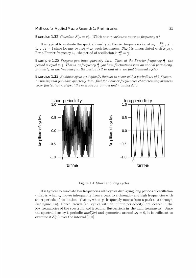
E xample 1.25 Suppose you have quarterly data. Then at the Fourier frequency π2 , the period is equal to 4. That is, at frequency π2 you have fl uctuations with an annual periodicity.Similarly, at the frequency π, the period is 2 so that at π we fi nd biannual cycles.

E xercise 1.33 Business cycle are typically thought to occur with a periodicity of 2-8 years.Assuming that you have quarterly data, fi nd the Fourier frequencies characterizing business cycle fl uctuations. Repeat the exercise for annual and monthly data.

short periodicity

time

A

m p l i t u r e o f c y c l e s

0-1.0

-0.5

0.0

0.5

1.0long periodicity

time

A

m p l i t u r e o f c y c l e s

0-1.0

-0.5

0.0

0.5

1.0

Figure 1.4: Short and long cycles

It is typical to associate low frequencies with cycles displaying long periods of oscillation

- that is, when yt moves infrequently from a peak to a through - and high frequencies withshort periods of oscillation - that is, when yt frequently moves from a peak to a through(see figure 1.4). Hence, trends (i.e. cycles with an infinite periodicity) are located in thelow frequencies of the spectrum and irregular fluctuations in the high frequencies. Sincethe spectral density is periodic mod(2π) and symmetric around ω j = 0, it is sufficient toexamine it S (ω) over the interval [0, π].



24

E xercise 1.34 Show that S (ω j) = S (−ω j).

Example 1.26 Suppose {yt(κ )} is iid (0,σ2y). Then ACF y(τ ) = σ2y for τ = 0 and zero

otherwise and S y(ω j) = σ2

2π ∀ω j. That is, the spectral density of an iid process is constant for all ω ∈ [0,π].

Frequency

S p e c t r a l

p o w e r

-3 -2 -1 0 1 2 3

9.5

9.6

9.7

9.8

9.9

10.0

Figure 1.5: Spectral density

E xercise 1.35 Consider a stationary AR(1) process {yt(κ )} with autoregressive coe ffi cient equal to A. Calculate the autocovariance function of the process. Show that the spectral density is increasing monotonically as ω j → 0.

E xercise 1.36 Consider a stationary MA(1) stochastic process {yt(κ )} with MA coe ffi cient equal to D. Calculate the autocovariance function and the spectral density of yt. Show its shape when D > 0 and when D < 0.

Economic time series have a typical bell shaped spectral density (seefi

gure1

.5) witha large portion of the variance concentrated in the lower part of the spectrum. Given theresult of exercise 1.35 it is therefore reasonable to assume that most of economic time seriescan be represented with relatively simple AR processes.

The definitions we have given are valid for univariate processes, but can be easily ex-tended to vector of stochastic processes.




Definition 1.28 (Spectral density matrix): The spectral density matrix of an m ×1 vector of stationary processes {yt(κ )}∞t=−∞ is S y(ω j) = 1

2π

Pτ ACF y(τ )e−iωjτ where

S (ω j) =

S y1y1(ω j) S y1y2(ω j) . . . S y1ym(ω j)

S y2y1(ω j) S y2y2(ω j) . . . S y2ym(ω j). . . . . . . . . . . .

S ymy1(ω j) S ymy2(ω j) . . . S ymym(ω j)

The elements on the diagonal of the spectral density matrix are real while the elementsoff -the diagonal are typically complex. A measure of the strength of the relationship betweentwo series at frequency ω j is given by the coherence.

Definition 1.29 Consider a bivariate stationary process {(y1t(κ ), y2t(κ ))}. The coherence

between {(y1t(κ ), y2t(κ ))} at freqeuncy ω j is Co(ω j) =|S y1,y2(ωj)|√

S y1,y1(ωj)S y2,y2(ωj).

The coherence is the frequency domain version of the correlation coefficient and measuresthe strength of the association between y1t and y2t at ω j . Notice that Co(ω j) is a real valuedfunction where |y| indicates the real part (or the modulus) of complex number y.

E xample 1.27 Suppose yt = D(`)et where et ∼ iid (0,σ2e). Then it is immediate to show that the coherence between et and yt is one at all frequencies. Suppose, on the other hand,that Co(ω j) monotonically declines to zero as ω j moves from 0 to π. Then yt and et have similar low frequency components and di ff erent high frequency ones.

E xercise 1.37 Suppose that et ∼ iid (0,σ2e) and let yt = et+Det−1. Calculate Coyt,et(ω j).

Interesting transformations of the spectrum of yt can be obtained with the use of filters.

Definition 1.30 A fi lter is a linear transformation of a stochastic process, i.e. if yt =B (`)et, et ∼ iid (0,σ2

e), then B (`) is a fi lter.

A moving average (MA) process is therefore a filter since it linearly transforms a whitenoise into another process. In general, stochastic processes can be thought of as filteredversions of some white noise process (the news). To study the spectral properties of filteredprocesses let CGF e(z) be the covariance generating function of et. Then the covariancegenerating function of yt is CGF y(z) = B (z)B (z−1)CGF e(z) = |B (z)|2CGF e(z) where |B (z)|is the modulus of B (z).

E xample 1.28 Suppose that et ∼ iid (0,σ2e) so that its spectrum is S e(ω j) = σ2

2π , ∀ω j.Consider now the process yt = D(`)et where D(`) = D0 + D1` + D2`2 + . . .. It is typical to interpret D(`) as the response function of yt to a unitary change in et. Then S y(ω j) =|D(e−iωj)|2S e(ω j) where |D(e−iωj )|2 = D(e−iωj )D(eiωj) and D(e−iωj) =

Pτ Dτ e

−iωjτ mea-sures the e ff ect of a unitary change in et at frequency ω j.



26

Example 1.29 Suppose that yt = a0 + a1t + D(`)et where et ∼ iid (0,σ2e). Since yt

has a (linear) trend is not stationary in levels and S (ω j) does not exists. Di ff erencing the process we have yt

−yt−1 = a1 + D(`)(et

−et−1) so that yt

−yt−1 is stationary if et

−et−1

is a stationary and all the roots of D(`) are greater than one in absolute value. If these conditions are met the spectrum of yt − yt−1 is well de fi ned and equals |D(e−iω j)|2S ∆e(ω j).

The quantity B (e−iωj ) is called transfer function of the filter. Various functions of this quantity are of interest in time series analysis. For example, |B (e−iωj)|2, the squaremodulus of the transfer function, measures the change in variance of et induced by thefilter. Furthermore, since B (e−iωj) is, in general, complex two alternative representationsof the transfer function of the filter exist. The first decomposes it into its real and complexpart, i.e. B (e−iωj ) = B †(ω j) + iB ‡(ω j) where both B † and B ‡ are real. Then the phase

shift is P h(ω j) = tan−1[−B‡(ωj)B†(ωj)

], measures how much the lead-lag relationships in et are

altered by the filter. The second can be obtained using the polar representation B (e−iωj ) =

Ga(ω j)e−iPh(ωj) where Ga(ω j) is the gain. Here Ga(ω j) = |B (e−iωj)| measures the changein the amplitude of cycles induced by the filter.

Low Pass

Frequency0.0 1.5 3.0

0.00

0.25

0.50

0.75

1.00

1.25High Pass


0.00

0.25

0.50

0.75

1.00

1.25Band Pass


0.00

0.25

0.50

0.75

1.00

1.25

Figure 1.6: Filters

Filtering is an operation frequently performed in every day life (e.g. tuning a radio on

a station filters out all other signals (waves)). Several types of filters are used in modernmacroeconomics. Figure 1.6 presents three general types of filters: a low pass, a high pass,and a band pass. A low pass filter leaves the low frequencies of the spectrum unchangedbut wipes out high frequencies. A high pass filter does exactly the opposite. A band passfilter is a combination of a low pass and a high pass filters: it wipes out very high and verylow frequencies and leaves unchanged frequencies in middle range.




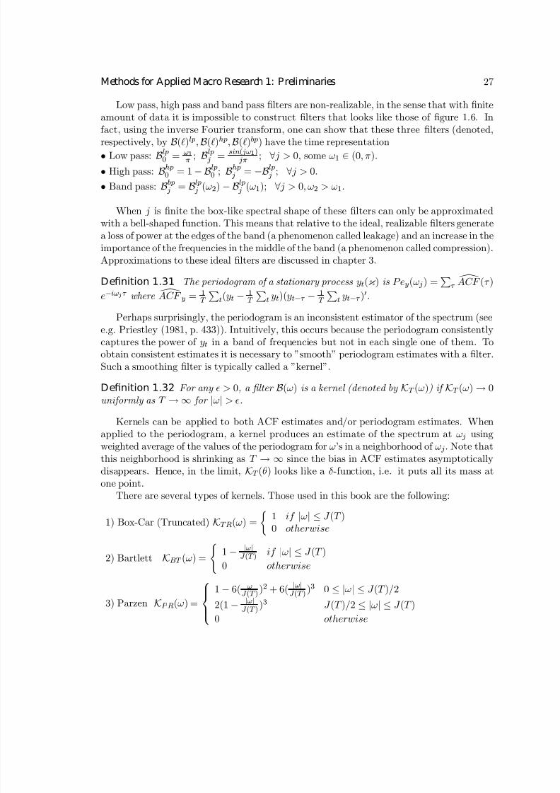
Low pass, high pass and band pass filters are non-realizable, in the sense that with finiteamount of data it is impossible to construct filters that looks like those of figure 1.6. Infact, using the inverse Fourier transform, one can show that these three filters (denoted,

respectively, by B (`)lp, B (`)hp, B (`)bp) have the time representation• Low pass: B lp0 = ω1

π; B lp j = sin( jω1)

jπ ; ∀ j > 0, some ω1 ∈ (0,π).

• High pass: B hp0 = 1− B lp0 ; B hp j = −B lp j ; ∀ j > 0.

• Band pass: B bp j = B lp j (ω2) − B lp j (ω1); ∀ j > 0,ω2 > ω1.

When j is finite the box-like spectral shape of these filters can only be approximatedwith a bell-shaped function. This means that relative to the ideal, realizable filters generatea loss of power at the edges of the band (a phenomenon called leakage) and an increase in theimportance of the frequencies in the middle of the band (a phenomenon called compression).Approximations to these ideal filters are discussed in chapter 3.

Definition 1.31 The periodogram of a stationary process yt(κ ) is P ey(ω j) =Pτ [ ACF (τ )

e−iωjτ where [ ACF y = 1T

Pt(yt − 1

T

Pt yt)(yt−τ − 1

T

Pt yt−τ )0.

Perhaps surprisingly, the periodogram is an inconsistent estimator of the spectrum (seee.g. Priestley (1981, p. 433)). Intuitively, this occurs because the periodogram consistentlycaptures the power of yt in a band of frequencies but not in each single one of them. Toobtain consistent estimates it is necessary to ”smooth” periodogram estimates with a filter.Such a smoothing filter is typically called a ”kernel”.

Definition 1.32 For any ² > 0, a fi lter B (ω) is a kernel (denoted by KT (ω)) if KT (ω) → 0uniformly as T → ∞ for |ω| > ².

Kernels can be applied to both ACF estimates and/or periodogram estimates. Whenapplied to the periodogram, a kernel produces an estimate of the spectrum at ω j usingweighted average of the values of the periodogram for ω’s in a neighborhood of ω j. Note thatthis neighborhood is shrinking as T → ∞ since the bias in ACF estimates asymptoticallydisappears. Hence, in the limit, KT (θ) looks like a δ -function, i.e. it puts all its mass atone point.

There are several types of kernels. Those used in this book are the following:

1) Box-Car (Truncated) KTR(ω) =

½1 if |ω| ≤ J (T )0 otherwise

2) Bartlett KBT (ω) = ( 1−|ω|

J (T ) if |ω| ≤ J (T )0 otherwise

3) Parzen KPR(ω) =

1− 6( ωJ (T ))2 + 6( |ω|

J (T ))3 0 ≤ |ω| ≤ J (T )/2

2(1− |ω|J (T )

)3 J (T )/2 ≤ |ω| ≤ J (T )

0 otherwise



28

4) Quadratic spectral KQS (ω) = 2512π2ω2

(sin(6πω/5)6πω/5 − cos(6πω/5))

Bartlett

Lags

S p e c t r a l p o w e r

-25 0 25-0.25

0.00

0.25

0.50

0.75

1.00

1.25

Quadratic Spectral

Lags

S p e c t r a l p o w e r

-25 0 25-0.25

0.00

0.25

0.50

0.75

1.00

1.25

Figure 1.7: Kernels

Here J (T ) is a truncation point, which typically is a function of the sample size T . Notethat the quadratic spectral kernel has no truncation point. However, for this kernel it isuseful to define the first time that KQS crosses zero (call it J ∗(T )) and this point will play

the same role as J (T ) in the other three kernels.The Barlett kernel and the quadratic spectral kernel are the most popular ones. TheBartlett kernel has the shape of a tent with width 2J (T ). To insure consistency of the

spectral estimates, it is typically to choose J (T ) so that J (T )T → 0 as T → ∞. In figure

1.7 we have selected J(T)=20. The quadratic spectral kernel has the form of a wave withinfinite loops, but after the first crossing, side loops are small.

E xercise 1.38 Show that the coherence estimator Co(ω) =| bS y1,y2(ω)|q bS y1,y1 bS y2,y2 is consistent,

where

bS yi,yi0 = 1

2π

PT −1τ =−T +1

[ ACF y1,yi0 (τ )KT (ω)e−iωτ , KT (ω) is a kernel and i, i0 = 1, 2.

While for most part of this book we consider stationary processes, we will also deal withprocesses which are only locally stationary (e.g. processes with time varying coefficients).For these processes, the spectral density is not defined. However, it is possible to define a”local” spectral density and practically all the properties we have described here apply alsoto this alternative construction. For details, see Priestley (1980, chapter 11).

methods for applied macroeconomics research - ch1

Documents