methods for analysis and control of dynamical systems ...o.sename/docs/auto_e7... · methods for...
TRANSCRIPT

Methods for analysis and control of dynamical systems
Lecture 3: tools for performance analysis
GIPSAlab Control Systems department Grenoble INP-CNRS
ENSE3-BP 4638402 Saint Martin d'Hères Cedex, FRANCE
Olivier SENAME

© Olivier Sename 2009
Outline
Introduction Time-domain performance criteria Frequency-domain performance criteria Sensitivity function analysis Towards robustness analysis

© Olivier Sename 2009
Goodwin et al, 01 : “Success in control engineering depends on taking a holistic viewpoint. Some of the issues are :
plant, i.e. the process to be controlled
objectives
sensors
actuators
communications
computing
algorithms
architectures and interfacing
accounting for disturbances and uncertainties …”
Network ControlledSystems
THE CONTROL SYSTEM DESIGN

© Olivier Sename 2009
Skogestad and Postlewaite, 96: “The process of designing a control system makes many demands of the engineering team. The steps to be followed are:
Plant study and modelling
Determination of sensors and actuators (measured and controlled outputs, control inputs)
Performance specifications
Control design
Simulation tests
Implementation ….”
THE CONTROL SYSTEM DESIGN

© Olivier Sename 2009
THE CONTROL SYSTEM DESIGN
Steps :
Controlmodel
Industrial and academic
performances specifications
Controlsynthesis
Identitification and/or Modelling: 1. Formulate a nonlinear state-space model based on physical knowledge.2. Determine the steady-state operating point about which to linearize.3. Introduce deviation variables and linearize the model.
needs good system knowledgeneeds criteria choice
Us of various methods:Internal model control, Pole
placementPredictive control, LQ control
Hinf control …..

© Olivier Sename 2009
THE CONTROL SYSTEM DESIGN
objective of a control system : make the system output behave in a desired way by manipulating the plant input.
The regulator problem is to reject (or reduce) theeffect of some disturbance or measurement noise on the output y.
The servo problem is to keep the output close to a given reference input r

© Olivier Sename 2009
THE CONTROL SYSTEM DESIGN
Actuators System
Sensors
Controller
Controlsignal
Disturbances
Measurementnoise
Reference
In practice the feedback control loop is of the form :

© Olivier Sename 2009
FEEDBACK STRUCTURE
« Classical » one degree-of-freedom structure
Two degree-of-freedom structure
RST structure
SOME CONTROL STRUCTURES
In the following: only SISO (Single Input Single Output) systemsare considered, for sake of simplicity.Most of results can be extended to MIMO systems (Multi Input Multi Output)

© Olivier Sename 2009
FEEDBACK STRUCTURE
Classical one degree-of-freedom structure
K(s) G(s)r(t) y(t)
n(t)
di(t) dy(t)
+
-+
+ +
+
++
PLANT = G(s)CONTROLLER = K(s) FEEDBACK
reference
Inputdisturbance
Outputdisturbance
Output
Measurementnoise
uP(t)
Control Input
u(t)
Plant Input

© Olivier Sename 2009
FEEDBACK STRUCTURE
Two degree-of-freedom structure
K(s)
G(s)r(t) y(t)
n(t)
di(t) dy(t)
+
-+
+ +
+
++
Kp(s)
FEEDBACKFEEDFORWARD
Improves tracking performance

© Olivier Sename 2009
PERFORMANCE ANALYSIS
Objectives of any control system :
shape the response of the system to a given reference and get (or keep) a stable system in closed-loop, with desired performances, while minimising the effects of disturbances and measurement noises, and avoiding actuators saturation, this despite of modelling uncertainties, parameter changes or change of operating point.

© Olivier Sename 2009
PERFORMANCE ANALYSIS
Nominal stability (NS): The system is stable with the nominal model (no model uncertainty)
Nominal Performance (NP): The system satisfies the performance specifications with the nominal model (no model uncertainty)
Robust stability (RS): The system is stable for all perturbed plants about the nominal model, up to the worst-case model uncertainty(including the real plant)
Robust performance (RP): The system satisfies the performance specifications for all perturbed plants about the nominal model, up to the worst-case model uncertainty (including the real plant).
Objectives of any control system

© Olivier Sename 2009
Outline
Introduction Time-domain performance criteria Frequency-domain performance criteria Sensitivity function analysis Towards robustness analysis

© Olivier Sename 2009
PERFORMANCE ANALYSIS
Time domain performances
Classical performance indices
Steady-state offset: the difference between the final value and the desired final value,this offset is usually required to be small.
Rise time : the time, usually required to be small, that it takes for the output to first reach 90 % of its final value
Settling time : the time after which the output remains within 5 % of its final value, which is also usually required to be small.
Overshoot: the peak value divided by the final value : should typically be 1.2 (20 %) or less
Decay ratio: the ratio between the second and first peaks, which should typically be 0.3 or less

© Olivier Sename 2009
PERFORMANCE ANALYSIS
Time domain performances
Risetime
Settlingtime
Peakvalue

© Olivier Sename 2009
PERFORMANCE ANALYSIS
Decay ratio Steady state errors
Stepinput
Rampinput
© Olivier Sename 2009
PERFORMANCE ANALYSIS
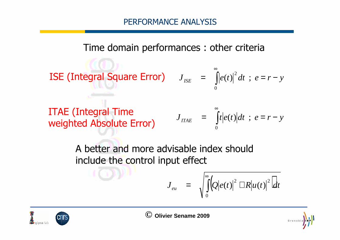
Time domain performances : other criteria
ISE (Integral Square Error) yredtteJ ISE −== ∫∞
; )(0
2
A better and more advisable index shouldinclude the control input effect
( )∫∞
+=0
22)()( dttuRteQJeu
ITAE (Integral Time weighted Absolute Error)
yredttetJ ITAE −== ∫∞
; )(0

© Olivier Sename 2009
Outline
Introduction Time-domain performance criteria Frequency-domain performance criteria Sensitivity function analysis Towards robustness analysis

© Olivier Sename 2009
PERFORMANCE ANALYSIS
Frequency performance criteria
K(s) G(s)r(t) y(t)
n(t)
di(t) dy(t)
+
-+
+ +
+
++
PLANT = G(s)CONTROLLER = K(s)
reference
Inputdisturbance
Outputdisturbance
Output
Measurementnoise

© Olivier Sename 2009
PERFORMANCE ANALYSIS
Frequency domain performances:
Stability
The closed-loop sytem isinternally stable iff all the transfer functions previouslydefined are stable« roots of the Characteristicpolynomial »

© Olivier Sename 2009
PERFORMANCE ANALYSIS
This requires closed-loop stability
1. The poles of the closed-loop system are evaluated. The system is stable if and
only if all the closed-loop poles are in the open left-half plane (LHP) (that is, poles
on the imaginary axis are considered “unstable”). The poles are also equal to the
eigenvalues of the state-space matrix A, and this is usually how the poles are
computed numerically.
2. The frequency response (including negative frequencies) of L(jw) is plotted in the
complex plane and the number of encirclements it makes of the critical point (-1)
is counted. By Nyquist’s stability criterion closed-loop stability is inferred by
equating the number of encirclements to the number of open-loop unstable poles
(RHP-poles).
o180)(;1)( 180180 −=∠< ωω jLjL

© Olivier Sename 2009
PERFORMANCE ANALYSIS
Sensitivity functions
)()()(1
1)(
)()()(1
1)(
iy
iy
KGdKnKdKrsGsK
su
GdGKndGKrsKsG
sy
−−−+
=
+−++
=
The output & the control input satisfy the following equations :
Firstly, SISO case
Outputdisturbance
K(s) G(s)r(t) y(t)
n(t)
di(t)dy(t)
+
-+
+ +
+
++
reference
Inputdisturbance
Output
Measurementnoise
u(t)e(t)

© Olivier Sename 2009
PERFORMANCE ANALYSIS
Frequency domain performances: Sensitivity functions
)()()(1
1)(
)()()(1
1)(
KnKdKGdKrsGsK
su
GKndGdGKrsKsG
sy
yi
yi
−−−+
=
−+++
=
)()(1
1)(
sKsGsS
+=Sensitivity
)()(1
)()()(
sKsG
sKsGsT
+=Complementary
Sensitivity
Let us define the well known sensitivity functions:
Loop transfer function )()()( sGsKsL =

© Olivier Sename 2009
PERFORMANCE ANALYSIS
Frequency domain performances: criteria
GAIN, PHASE, DELAY and MODULE MARGINS
The gain margin indicates the additional gain that would take the closedloop to the critical stability condition
The phase margin quantifies the pure phase delay that should be addedto achieve the same critical stability condition
The delay margin quantifies the maximal delay that should be addedin the loop to achieve the same critical stability condition
The module margin quantifies the minimal distance between the curveand the critical point (-1,0j): this is a robustness margin
© Olivier Sename 2009
PERFORMANCE ANALYSIS
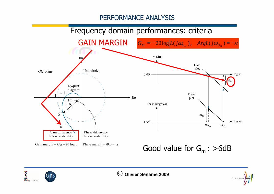
Frequency domain performances: criteria
GAIN MARGIN
Good value for Gm : >6dB
πωω −=−= )(,)(log20MM GGM jArgLjLG

© Olivier Sename 2009
PERFORMANCE ANALYSIS
Frequency domain performances: criteria
PHASE MARGIN
Good value for Φm : > 30/40°
1)(),(, 00 ==+=Φ ΦΦ MMjLjArgLM ωωϕϕπ

© Olivier Sename 2009
PERFORMANCE ANALYSIS
Frequency domain performances: criteria
DELAY MARGIN :acceptable pure time-delay before instability
M
M
Φ
Φ=∆ω
τ
© Olivier Sename 2009
PERFORMANCE ANALYSIS
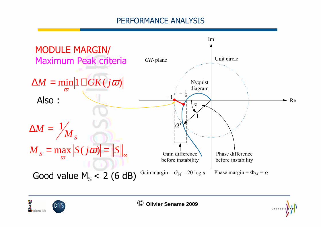
MODULE MARGIN/Maximum Peak criteria
)(1min ωω
jGKM +=∆
∞==
=∆
SjSM
MM
S
S
)(max
1
ωω
Also :
Good value MS < 2 (6 dB)

© Olivier Sename 2009
PERFORMANCE ANALYSIS
Advantage: good module margin implies good gain and phase margins
SS
S
MPM
M
MGM
1 and
1≥
−≥
For MS=2, then GM>2 and PM>30°
Last one : )(max ωω
jTM T =
Good value MT < 1.5 (3.5 dB)

© Olivier Sename 2009
PERFORMANCE ANALYSIS
The MODULE MARGIN is a robustness margin.
Indeed, the sensitivity function allows to qualify the robustness of the control system, as
)()(1
)()(
sGsK
sGsKTBF +
=
SMM 1=∆
Closed-loop transfer function
Influence of plant modelling errors on the CL transfer function G
G
sGsKT
T
BF
BF ∆+
=∆)()(1
1
Sensitivity function

© Olivier Sename 2009
PERFORMANCE ANALYSIS
Bandwidth
The concept of bandwidth is very important in understanding the benefits and
trade-offs involved when applying feedback control. Above we considered peaks
of closed-loop transfer functions, which are related to the quality of the response.
However, for performance we must also consider the speed of the response, and
this leads to considering the bandwidth frequency of the system.
In general, a large bandwidth corresponds to a faster rise time, since high
frequency signals are more easily passed on to the outputs. A high bandwidth also
indicates a system which is sensitive to noise and to parameter variations.
Conversely, if the bandwidth is small, the time response will generally be slow,
and the system will usually be more robust.

© Olivier Sename 2009
PERFORMANCE ANALYSIS
Bandwith :
Loosely speaking, bandwidth may be defined as the frequency range [w1,
w2] over which control is effective. In most cases we require tight control
at steady-state so w1=0, and we then simply call w2 the bandwidth.
The word “effective” may be interpreted in different ways : globally it
means benefit in terms of performance.
Definition1: The (closed-loop) bandwidth, wS, is the frequency where
|S(jw)| crosses –3dB (1/√2) from below.
Remark: |S|<0.707, frequency zone, where e/r = -S is reasonably small

© Olivier Sename 2009
PERFORMANCE ANALYSIS
Another interpretation: when it changes the output response.
As y=Tr, T must be sufficiently large
Definition2: The bandwidth (in term of T), wT, is the frequency where
|T(jw)| crosses –3dB (1/√2) from above.
Remark: In most cases, the two definitions in terms of S and T yield
similar values for the bandwidth. In other cases, the situation is
generally as follows. Up to the frequency wS, |S| is less than 0.7, and
control is effective in terms of improving performance. In the frequency
range [wS, wT] control still affects the response, but does not improve
performance. Finally, at frequencies higher than wT, we have S ≅ 1 and
control has no significant effect on the response.

© Olivier Sename 2009
PERFORMANCE ANALYSIS
The gain crossover frequency :
Definition3: The bandwidth (crossover frequency), wC, is the frequency
where |L(jw)| crosses 1 (0dB), for the first time, from above.
Remark:It is easy to compute and usually gives
wS < wC < wT
Note that the rise time can often be evaluated as :
Trt ω
3.2=

© Olivier Sename 2009
Outline
Introduction Time-domain performance criteria Frequency-domain performance criteria Sensitivity function analysis Towards robustness analysis

© Olivier Sename 2009
PERFORMANCE ANALYSIS
Input and Output Performance analysis using the Sensitivity functions
The output & the control input performances can bestudied through 4 « sensitivity » functions only.
Outputdisturbance
K(s) G(s)r(t) y(t)
n(t)
di(t)dy(t)
+
-+
+ +
+
++
reference
Inputdisturbance
Output
Measurementnoise
u(t)e(t)

© Olivier Sename 2009
PERFORMANCE ANALYSIS
KS(s)
-T(s)
-KS(s)
-KS(s)
Σu(t)
r(t)
di(t)
dy(t)
n(t)
Input performance
)()()(1
1)(
)()()(1
1)(
iy
iy
KGdKnKdKrsGsK
su
GdGKndGKrsKsG
sy
−−−+
=
+−++
=
Output performance
T(s)
SG(s)
S(s)
-T(s)
Σy(t)
r(t)
di(t)
dy(t)
n(t)

© Olivier Sename 2009
PERFORMANCE ANALYSIS
)()()(1
1)( KnKdKGdKr
sGsKsu yi −−−
+=
The effect of the input disturbance di(t) on the plant input u(t)+ di(t) (actuator) can be made « small » by making the sensitivity function S(s) small
The transfer function KS(s) should be upper boundedso that u(t) does not reach the physical constraints, even for a large reference r(t)
The effect of the measurement noise n(t) on the plantinput u(t) can be made « small » by making the sensitivity function KS(s) small (in High Frequencies)
KS(s)
-T(s)
-KS(s)
-KS(s)
Σu(t)
r(t)
di(t)
dy(t)
n(t)
Input performance

© Olivier Sename 2009
PERFORMANCE ANALYSIS
)()()(1
1)( GKndGdGKr
sKsGsy yi −++
+=
The plant output y(t) can track the reference r(t) by making the complementary sensitivity function T(s) equal to 1. (servo pb)
The effect of the output disturbance dy(t) (resp. input disturbance di(t) ) on the plant output y(t) can be made « small » by making the sensitivity function S(s) (resp. SG(s) ) « small »
The effect of the measurement noise n(t) on the plant output y(t) can be made « small » by making the complementary sensitivity function T(s) « small »
Some trade-offs are to be looked for
BUT S(s) + T(s) = 1
Output performance
T(s)
SG(s)
S(s)
-T(s)
Σy(t)
r(t)
di(t)
dy(t)
n(t)

© Olivier Sename 2009
PERFORMANCE ANALYSIS
These trade-offs can be reached if one aims :• to reject the disturbance effects in low frequency• to minimize the noise effects in high frequency
We will require:• S and SG to be small in low frequencies to reduce the load (output and input) disturbance effects on the controlled output
• T and KS to be small in high frequencies to reduce the effects of measurement noises on the controlled output and on the control input (actuator efforts)
KS(s)
-T(s)
-KS(s)
-KS(s)
Σu(t
r(t)
di(t)
dy(t)
n(t)
T(s)
SG(s)
S(s)
-T(s)
Σy(t)
r(t)
di(t)
dy(t)
n(t)

© Olivier Sename 2009
PERFORMANCE ANALYSIS
Position control of a DC motor, using internal speed feedback
A 1/kv 1/(τp+1) 1/(np) U0/(2Π)
1/kv1/kvRCp/(RCp+1)
Ve +
-
+
-
VsxΩ

© Olivier Sename 2009
PERFORMANCE ANALYSIS
Frequency (rad/sec)
Sin
gula
r V
alue
s (d
B)
S
10-2 10-1 100 101 102-80
-60
-40
-20
0
20
Frequency (rad/sec)
Sin
gula
r V
alue
s (d
B)
T
10-2 10-1 100 101 102-20
-15
-10
-5
0
5
Frequency (rad/sec)
Sin
gula
r V
alue
s (d
B)
KS
10-2 10-1 100 101 102-80
-60
-40
-20
0
Frequency (rad/sec)
Sin
gula
r V
alue
s (d
B)
SG
10-2 10-1 100 101 102-15
-10
-5
0
5
10
Good disturbance rejection
Good noise rejection
Bad: control input sensitive to noise
Bad: Input disturbance (di)are not rejected
WB=15.3 rad/s WBT=27.1 rad/s

© Olivier Sename 2009
PERFORMANCE ANALYSIS
0 1 2 3 4 5 6 7 8 9 100
0.5
1
1.5
2
2.5
reference step
Output disturbance dy
Input disturbance di

© Olivier Sename 2009
PERFORMANCE ANALYSIS
WS=15.3 rad/s
WT=27.1 rad/s
Bandwith :
Wc=21 rad/s
And it holds :
wS < wC < wTPhase margin= 72.4 degGain margin = infModule margin < 1.5 db, MT=0.5db
Frequency (rad/sec)
Pha
se (
deg)
; M
agni
tude
(dB
)
Bode Diagrams
-100
-50
0
50
100From: U(1)
100 101 102-180
-160
-140
-120
-100
-80
To: Y
(1)
ωc=27 rad/s
Open-Loop Phase (deg)
Ope
n-Lo
op G
ain
(dB
)
Nichols Charts
-180 -170 -160 -150 -140 -130 -120 -110 -100 -90-150
-100
-50
0
50
100From: U(1)
To: Y
(1)
>>[Gm,Pm,W180,Wc]=margin(sys)>> MT=hinfnorm(T)MS=hinfnorm(S);

© Olivier Sename 2009
PERFORMANCE ANALYSIS
WS=15.3 rad/s
WT=27.1 rad/s
Bandwith :
Wc=21 rad/s
It holds :
mstT
r 853.2 == ω
1 1.05 1.1 1.15 1.2 1.25 1.3 1.35 1.4 1.45 1.50
0.2
0.4
0.6
0.8
1
1.2
1.4
rise time
and :
wS < wC < wT

© Olivier Sename 2009
% Determination of the sensitivity fucntionsG %% plant model LTI modelK %% controller LTI modelL=series(G,K) % Loop transfer function L=GKS=inv(1+L); % S= 1/(1+L)poleS=pole(S)T= feedback(L,1)poleT=pole(T)%%%%%%%%%%%%%%%%%%%%%%%%%%%%%%%%%%%%%%%%%%%%%%%%%%%%%%%%%SG=S*G;;poleSG=pole(SG)KS=K*S;poleKS=pole(KS)%%%%w=logspace(-2,2,500);subplot(2,2,1), sigma(S,w), title('Sensitivity funct ion')subplot(2,2,2), sigma(T,w), title('Complementary se nsitivity function')subplot(2,2,3), sigma(SG,w), title('Sensitivity*Pla nt')subplot(2,2,4), sigma(KS,w), title('Controller*Sens itivity')
EXAMPLE using MATLAB

© Olivier Sename 2009
EXAMPLE
10-2
10-1
100
101
102
-80
-70
-60
-50
-40
-30
-20
-10
0
10Sensitivity function
Frequency (rad/sec)
Sin
gula
r V
alue
s (d
B)
10-2
10-1
100
101
102
-60
-50
-40
-30
-20
-10
0
Complementary sensitivity function
Frequency (rad/sec)
Sin
gula
r V
alue
s (d
B)
10-2
10-1
100
101
102
-45
-40
-35
-30
-25
-20
-15
-10
-5Sensitivity*Plant
Frequency (rad/sec)
Sin
gula
r V
alue
s (d
B)
10-2
10-1
100
101
102
-40
-35
-30
-25
-20
-15
-10
-5
0
5
10
15Controller*Sensitivity
Frequency (rad/sec)
Sin
gula
r V
alue
s (d
B)
SensitivityfunctionS
ComplementarySensitivityfunctionT
SensitivityfunctionSG
SensitivityfunctionKS
We
Wu

© Olivier Sename 2009
Outline
Introduction Time-domain performance criteria Frequency-domain performance criteria Sensitivity function analysis Towards robustness analysis

© Olivier Sename 2009
UNCERTAINTY AND ROBUSTNESS
A control system is robust if it is insensitive to differences between the actual system and the model of the system which was used to design the controller
Introduction: Skegestad & Postlewaite
A method: these differences are referred as model uncertainty.
The approach
determine the uncertainty set: mathematical representation
check Robust Stability
check Robust Performance
How to take into account the difference between the actual system and the model ?
A solution: using a model set BUT : very large problem and not exact yet

© Olivier Sename 2009
UNCERTAINTY AND ROBUSTNESS

© Olivier Sename 2009
UNCERTAINTY AND ROBUSTNESS
Robust Stability analysis: SISO case
∆I(s)
G(s)
+
+
u∆y∆
u zLet us consider the case :
The loop transfer function is then: ;)( IIIIpp LwLwIGKKGL ∆+=∆+==
Therefore RS ⇔ System stable ∀ Lp. ⇔ Lp should not encircle the point -1
ω
ω
ω
∀<⇔
∀<+
⇔
∀+<⇔
1
,11
,1
Tw
L
Lw
LLwRS
I
I
I
Im
Re-1
LwI
L+1
)( ωjL