1

Methodological Fundamentalism: or why Batterman’s Different Notions of ‘Fundamentalism’ may

not make a Difference

William M Kallfelz1

June 19, 2006

Abstract

I argue that the distinctions Robert Batterman (2004) presents between

‘epistemically fundamental’ versus ‘ontologically fundamental’ theoretical

approaches can be subsumed by methodologically fundamental procedures. I

characterize precisely what is meant by a methodologically fundamental

procedure, which involves, among other things, the use of multilinear graded

algebras in a theory’s formalism. For example, one such class of algebras I

discuss are the Clifford (or Geometric) algebras. Aside from their being touted by

many as a “unified mathematical language for physics,” (Hestenes (1984, 1986)

Lasenby, et. al. (2000)) Finkelstein (2001, 2004) and others have demonstrated

that the techniques of multilinear algebraic ‘expansion and contraction’ exhibit a

robust regularizablilty. That is to say, such regularization has been demonstrated

to remove singularities, which would otherwise appear in standard field-theoretic,

mathematical characterizations of a physical theory. I claim that the existence of

such methodologically fundamental procedures calls into question one of

Batterman’s central points, that “our explanatory physical practice demands that

we appeal essentially to (infinite) idealizations” (2003, 7) exhibited, for example,

by singularities in the case of modeling critical phenomena, like fluid droplet

formation. By way of counterexample, in the field of computational fluid

dynamics (CFD), I discuss the work of Mann & Rockwood (2003) and Gerik

Scheuermann, (2002). In the concluding section, I sketch a methodologically

fundamental procedure potentially applicable to more general classes of critical

phenomena appearing in fluid dynamics.

1 Committee of Philosophy and the Sciences, University of Maryland, College Park

Email.: wkallfel@umd.edu. Home page: http://www.glue.umd.edu/~wkallfel

2

I. Introduction

Robert Batterman (2005) distinguishes between “ontologically fundamental” and

“epistemically fundamental” theories. The aim of former is to “get the metaphysical

nature of the systems right,” (19) often at the expense of being explanatorily inadequate.

Fundamentally explanatory issues involving the universal dynamical behavior of critical

phenomena,2 for instance, cannot be dealt with by the ontologically fundamental theory.

Epistemologically fundamental theories, on the other hand, seek to achieve such an

explanatory aim accounting for such universal behavior, at the expense of suppressing (if

not outright misrepresenting) a physical system’s fundamentally ontological features.

In the case of critical phenomena such as drop formation,3 even in accounts of

more fine-grained resolutions of the scaling similarity solution for the Navier-Stokes

equations (which approximate a fluid as a continuum), “we must appeal to the non-

Humean similarity solution (resulting from the singularity) of the idealized continuum

Navier-Stokes theory.” (20) In a more general sense, though “nature abhors a

singularity…without them one cannot characterize, describe, and explain the emergence

of new universal phenomena at different scales.” (19)

In other words, we need the ontologically “false” but epistemically fundamental

theory to account for the ontologically true but epistemically lacking fundamental theory.

“[A] complete understanding (or at least an attempt) of the drop breakup problem

2Such critical phenomena exhibiting universal dynamical properties include, but are not limited to,

examples including fluids undergoing phase transitions under certain conditions favorable for modeling

their behavior using Renormalization Group methods, shock-wave propagation (phonons), caustic surfaces

occurring under study in the field of catastrophe optics, quantum chaotic phenomena, etc. 3 applied to the nanoscale jets analyzed by Landman & Mosely.

3

requires essential use of a ‘nonfundamental’ [i.e. epistemically fundamental] theory…the

continuum Navier-Stokes theory of fluid dynamics.” (18)

Batterman advocates this necessary coexistence of two kinds of fundamental

theories, which in my opinion, can be viewed as a refinement of his more general themes

presented in (2002). There, he argues that in the case of emergent phenomena,

explanation and reduction part company: the superseded theory T can still play an

essential role. That is to say, the superseding theory T/, though ‘deeply containing T ’ (in

some non-reductive sense) cannot adequately account for emergent and critical

phenomena alone, and thus enlists T in some essential manner. According to Batterman,

this produces a rift between reduction and explanation, insofar as one is forced to

accommodate an admixture of differing ontologies characterized by the respectively

superseding and superseded theories. In his later work, Batterman (2005) seems to imply

that epistemologically fundamental theories serve in a similarly necessary capacity in

terms of what he explains the superseded theories do, in the case of emergent phenomena

(2002).

I have critiqued (Kallfelz (2005b)) Batterman’s claims (2002, 2004) in a two-fold

manner: Batterman confuses a theory’s (mathematical) topology with its (metaphysical)

ontology. This confusion, in turn, causes him to reify unnecessarily certain notions of

singularities, in the explanatory role they play in the superseded theory. I argue here that

there exist methods of regularization in multilinear algebraic characterizations of

microphysical phenomena employed by theoretical physicists (Finkelstein (2002-2005),

Green (2000)) which seem to provide a truer ontological account for what goes on at the

4

microlevel, and bypass singularities that would otherwise occur in more conventional

mathematical techniques (not based on multilinear algebras).

I characterize such a notion of ‘fundamental’ arising in algebraic expansion and

contraction techniques as an example of a methodological fundamentalism: for it offers a

means of intertheoretic reduction which overcomes the singular cases Batterman seems to

reify (2002, 2004). In the case of fluid dynamics, mulitilinear algebras like Clifford

algebras have been recently applied by Gerik Scheuermann (2000), Mann & Rockwood

(2003), in their work on computational fluid dynamics (CFD). The authors show that

CFD methods involving the Clifford algebraic techniques are often applicable in the same

contexts as the Navier-Stokes treatment –minus the singularities. Such results imply that

methodological fundamentalism can, in the cases Batterman investigates, provisionally

sort out and reconcile epistemically and ontologically fundamental theories. Hence, pace

Batterman, they need not act in cross purposes.

II. Epistemological Versus Ontological Fundamentalism (Batterman, 2005)

Robert Batterman explains the motivation for presenting a distinction between

ontological versus epistemically fundamental theories:

I have tried to show that a complete understanding (or at least an attempt…) of

the drop breakup problem requires essential use of a ‘nonfundamental’

theory…the continuum Navier Stokes theory of fluid dynamics…[But] how can a

false (because idealized) theory such as continuum fluid dynamics be essential for

understanding the behaviors of systems that fail completely to exhibit the

principal feature of that idealized theory? Such systems [after all] are discrete in

nature and not continuous…I think the term ‘fundamental theory’ is

ambiguous…[An ontologically fundamental theory]…gets the metaphysical

nature of the system right. On the other hand…ontologically fundamental

theories are often explanatorily inadequate. Certain explanatory questions…about

the emergence and reproducibility of patterns of behavior cannot be answered by

5

the ontologically fundamental theory. I think that this shows…there is an

epistemological notion of ‘fundamental theory’ that fails to coincide with the

ontological notion. (2005, 18-19, italics added)

On the other hand, epistemically fundamental theories aim at a more comprehensive

explanatory account, often, however, at the price of introducing essential singularities.

For example, in the case of ‘universal classes’ of behavior of fluid-dynamical phenomena

exhibiting patterns like droplet formation:

Explanation of [such] universal patterns of behavior require means for eliminating

details that ontologically distinguish the different systems exhibiting the same

behavior. Such means are often provided by a blow-up or singularity in the

epistemically more fundamental theory that is related to the ontologically

fundamental theory by some limit. (ibid., italics added)

Obviously, any theory relying on a continuous topology4 harbors the possibility of

exhibiting singular behavior, depending on its domain of application.5 In the case of

droplet-formation, for example, the (renormalized) solutions to the (continuous) Navier-

Stokes Equations (NSE) exhibit singular behavior. Such singularities play an essential

explanatory role insofar as such solutions in the singular limit exhibit ‘self-similar,’ or

universal behavior, to the extent that only one parameter essentially governs the behavior

of the solutions to the NSEs in such a singular limit. Specifically, only the fluid’s

thickness parameter (neck radius h) governs the shape of the fluid near break-up,6 in the

asymptotic solution to the NSE (2004, 15):

4 I am borrowing from Batterman’s (2002) usage, in which he distinguishes the ontology, i.e. the primitive

entities stipulated by a physical theory, from its topology, or structure of its mathematical formalism. 5 This is of course due to the rich structure of continuous sets themselves admitting such effects. Consider,

for example, the paradigmatic example: f ∈(-∞, ∞)(-∞, ∞)

given by the rule: f(x) = 1/x . This obviously

produces an essential singularity at x = 0. 6 For fluids of low viscosities see Batterman (2004), n 12, p.16.

6

h(z/ ,t

/)

( ) ( ) ( )

( )β

α

ζ

ζ

tf

z

Htftzh

′

′=

′=′′,

z/= z- z0

t/= t- t0

(z0 , t0)

z

where: f(t/) is a continuous (dimensionless) function expressing the time-dependence of

the solution (t/= t- t0 is the measured time after droplet breakup t0).

α ,β are phenomenological constants to be determined.

H is a Haenkel function.7

One could understand the epistemically and ontologically fundamental theories as

playing analogous roles to Batterman’s (2002, 2003, 2004) previously characterized

superseded and superseding theories (T and T

/, respectively). Like in the case of the

superseded theory T, the epistemically fundamental theory offers crucial explanatory

insight, at the expense of mischaracterizing the underlying ontology of the phenomena

under study. Whereas, on the other hand, analogous to the case of the superseding theory

T /, the ontologically fundamental theory gives a more representative metaphysical

characterization, at the expense of losing its explanatory efficacy.8

7 I.e. belonging to a class of orthonormal special functions often appearing in solutions to PDEs describing

dynamics of boundary-value problems. 8 For instance, in the case of the breaking water droplet, the ontologically fundamental theory would be the

molecular-discrete one. But aside from practical limitations posed by the sheer intractability of the

computational complexity of such a quantitative account, the discrete-molecular theory, precisely because

it lacks the singular-asymptotic aspect, cannot depict the (relatively) universal character presented in the

asymptotic limit of the (renormalized) solutions to the NSE.

7

However, I argue that there are theoretical characterizations whose formalisms

can regularize or remove singularities from some of the fluid-dynamical behavior in a

sufficiently abstract and general manner, as to call into question the presumably essential

distinctions between epistemological and ontological fundamentalism. I call such formal

approaches “methodologically fundamental,” because of the general strategy such

approaches introduce, in terms of offering a regularizing procedure.9 Adopting such

methodologically fundamental procedures, whenever it is possible to do so,10

suggests

that Batterman’s distinctions may not be different theoretical kinds, but function at best as

different aspects of a unified methodological strategy. This calls into question the

explanatory pluralism Batterman appears to be advocating.

Similar to Gordon Belot’s (2003) criticism, I am also arguing that extending the

breadth and scope of theories in mathematical physics applied to the domains of critical

phenomena Batterman calls our attention to, goes a long way to qualify and diminish the

distinctions he makes. Belot argues that a richer and more mathematically rigorous

rendition of the superseding theory T / eliminates the necessity of one having to resort

simultaneously to the superseded theory T to characterize some critical phenomenon (or

class of phenomena) Φ. Like Belot, I also claim that multilinear algebraic techniques

abound which can regularize the singularities appearing in formalisms of T (or T / ).

Conversely, when representing such critical phenomena Φ, singularities can occur in T

9 In other words, this strategy should not be conceived of as a merely souped-up version of an ontologically

fundamental theory. The latter, according to Batterman, are stuck at the level of giving very detailed

accounts involving the particular features of the phenomena at the expense of accounting for generally

significant universal dynamical features shared, across the board, of many fundamentally distinct material

kinds (like in the case of different kinds of fluids exhibiting universally self-similar behavior, during critical

phase transitions.) 10

The generality of the methods do not imply that they are a panacea, ridding any theory’s formalism of

singularities.

8

(or T / ) when the latter are characterized by the more typically standard field-theoretic or

phase space methods alone.

However, the mathematical content of the techniques I investigate differs

significantly from those discussed by Belot (2003), who characterizes T / using the more

general and abstract theory of differentiable manifolds. He demonstrates that in

principle, all of the necessary features of critical phenomena Φ can be so depicted by the

mathematical formalism of superseding theory T / alone (2003, 23). Because the

manifold structure is continuous, this can (and does) admit the possibility of depicting

such critical phenomena Φ through complex and asymptotic singular behavior. In other

words, Belot is not fundamentally questioning the underlying theoretical topologies

typically associated with T and T /.11

Instead, he is questioning the need to bring the two

different ontologies of the superseded and superseding theories together, to adequately

account for Φ. Belot is questioning the presumed ontological pluralism that Batterman

advanced in his notion of an ‘asymptotic explanation’.12

11

I.e., differential equations on phase space, characterizable through the theory of differential manifolds. 12

Batterman (2003) responds:

I suspect that one intuition behind Belot’s …objection is…I [appear to be] saying that for genuine

explanation we need [to] appeal essentially to an idealization [i.e., the ontology of the superseded

theory T.] …In speaking of this idealization as essential for explanation, they take me to be

reifying [T’s ontology]…It is this last claim only that I reject. I believe that in many instances our

explanatory physical practice demands that we appeal essentially to (infinite) idealizations. But I

don’t believe that this involves the reification of the idealized structures.” (7)

It is, of course, precisely the latter claim “that we appeal essentially to (infinite) idealizations” that I take

issue with here, according to what the regularization procedures indicate. Batterman, however, cryptically

and subsequently remarks that: “In arguing that an account that appeals to the mathematical idealization is

superior to a theory that does not invoke the idealizations, I am not reifying the mathematics…I am

claiming that the ‘fundamental’ theory that fails to take seriously the idealized [asymptotic] ‘boundary’ is

less explanatorily adequate.” (8) In short, it seems that in his overarching emphasis of his interest in what

he considers to be novel accounts of scientific explanation (namely, of the asymptotic variety) he often

blurs the distinctions, and shifts emphasis between a theory’s ontology and its topology. It is precisely this

sort of equivocation, I maintain, that causes him to inadvertently reify mathematical notions like ‘infinite

idealizations.’ To put it another way, since it is safe to assume that the actual critical phenomena

9

I, on the other hand, pace Belot (2003) and Batterman (2002-2005) present an

alternative to the mathematical formalisms that both authors appeal to, which rely so

centrally on continuous topological structures.13

I show how discretely graded, and

ultimately finite-dimensional multi-linear geometric (Clifford) algebras can provide

accounts for some of the same critical phenomena Φ in a regularizable (singularity-free)

fashion.

Prior to describing the specific details of how to implement the strategy in the

case of critical phenomena exhibited in fluid dynamics, however, I make the following

disclaimer: I am definitely not arguing that the discrete, graded, multilinear Clifford-

algebraic methods share such a degree of universal applicability that they should supplant

the continuous, phase-space, infinite-dimensional differentiable manifold structure

constituting the general formalism of the theory of differential equations, whether

ordinary or partial. Certainly the empirical content of a specific problem domain

determines which is the ‘best’ mathematical structure to implement in any theory of

mathematical physics. By and large, such criteria are often determined essentially by

practical limitations of computational complexity.

We run into no danger, so long as we can carefully distinguish the

epistemological, ontological, and methodological issues vis-à-vis our choice of

mathematical formalism(s). If the choice is primarily motivated by practical issues of

computational facility, we can hopefully resist the temptation to reify our mathematical

maneuvering which would confuse the ‘approximate’ with the ‘fundamental’-- let alone

Batterman discusses are ultimately metaphysically finite, precisely how can one ‘appeal essentially to

(infinite) idealizations’ without inadvertently ‘reifying the mathematics?’ 13

Of course, in the case of Batterman, continuous structures comprise as well the ontology of the

epistemically fundamental theory: Navier-Stokes treats fluids as continua. In the case of Belot, the theory

of partial differential equations he presents relies fundamentally on continuous, differentiable manifolds.

10

confusing ontological, epistemological, and methodological senses of the latter notion.14

Even Batterman admits that “nature abhors singularities.” (2005, 20) So, I argue, should

we. The entire paradigm behind regularization procedures is driven by the notion that a

singularity, far from being an “infinite idealization we must appeal to” (Batterman 2003,

7), is a signal that the underlying formalism of theory is the pathological cause, resulting

in theory’s failure to provide information, in certain critical cases.

Far from conceding to some class of “asymptotic-explanations,” lending a picture

of the world of critical phenomena as somehow carved at the joints of asymptotic

singularities, we must instead search for regularizable procedures. This is precisely why

such an approach is methodologically fundamental: regularization implies some (weak)

form of intertheoretic reduction, as I shall argue below.

III. Clifford Algebraic Regularization Procedure: A Brief Overview

In this section, I summarize aspects of methods incorporating algebraic structures

frequently used in mathematical physics, leading up to and including the regularization

procedures latent in applications of Clifford Algebras. Because this material involves

some technical notions of varying degrees of specialty, I have provided for the interested

reader an Appendix at the end of this essay supplying all the necessary definitions and

brief explanations thereon.

14

I am, of course, not saying that there does not exist any connection whatsoever between a theory’s

computational efficacy and its ability to represent certain fundamentally ontological features of the

phenomena of interest. What that connection ultimately is (whether empirical, or some complex and

indirect logical blend thereof) I remain an agnostic.

11

I review here a few basic techniques involving (abstract algebraic) expansion and

contraction.15

Consider the situation in which the superceding theory T / is capable of

being characterized, in principle, by an algebra.16

Algebraic expansion denotes the

process of extending out from algebraically characterized T ′ to some *T ′ (denoted:

*TT ′→′ λ ) where λ is some fundamental parameter characterizing the algebraic

expansion (Finkelstein (2002) 4-8). The inverse procedure: TT ′=′→ *lim 0λ is

contraction.

The question becomes: how to regularize? In other words, which *T ′ should one

choose to guarantee a regular (i.e., non-singular) limit for any λ in the greatest possible

generality? Answer: expanding into an algebraic structure whose relativity group, i.e.,

the group of all its dynamical symmetries,17

is simple implies the Lie algebra depicting its

infinitesimal transformations is stable.18

This in turn entails greater reciprocity,19

i.e.,

“reciprocal couplings in the theory…reactions for every action.” (Finkelstein, 2002,10).

This is an instance of a methodologically fundamental procedure, which I summarize by

the following general necessary conditions:

15

For a concrete summary of Wigner’s (1952) analysis of algebraic expansion from the Galilean to the

Lorentz groups, for example, see Kallfelz (2005b), 16-17. 16

That is to say, a vector space with an associative product. For further details, see A.2 of the Appendix 17

In other words, the group of all actions in leaving their form of dynamical laws invariant (in the active

view) or the group of all ‘coordinate transformations’ preserving the tensor character of the dynamical laws

(in the ‘passive view.’) Also, see Defn. A.2.2 (Appendix A.2) for a description of simple groups. 18

For a brief description of stable Lie algebras, see the discussion following Defn A.2.4, section A.2,

Appedix. 19

For example, in the case of the Lorenz group, which is simple, it is maximally reciprocal in terms of its

fundamental parameters x, and t. That is to say, the form of Lorenz transformations (simplified in one

dimensional motion along the x-axes of the inertial frame F and F’ ) become x’ = x’(x,t) = γ(x – Vt) and t’ =

t’(x,t) = γ(t – Vx/c2) (where γ = (1-V

2/c

2)

-1/2 ). Hence both space x and time t couple when transforming

between inertial frames F, F’, as their respective transformations involve each other. On the other hand,

the Galilean group is not simple, as it contains an invariant subgroup of boosts. The Galilean

transformations are not maximally reciprocal, as x’ = x’(x,t) = x - Vt but t’ = t. x is a cyclic coordinate with

repect to transformation t’. Thus, when transforming between frames, x couples with respect to t but not

vice versa.

12

• Ansatz IIIa: If a procedure P for formulating a theory T in mathematical

physics is methodologically fundamental, then there exists some algebraically

characterized expansion *T ′ of T’s algebraic characterization (denoted by T /)

and some expansion parameter λ such that: *TT ′→′ λ . Then, trivially, *T ′ is

regularizable with respect to T / since TT ′=′→ *lim 0λ is well-defined (via the

inverse procedure of algebraic contraction).

• Ansatz IIIb: If *T ′ is an expansion of T /, then *T ′ ’s relativity group is simple,

which results in a stable Lie algebra d *T ′ , and whose set of observables in *T ′

is maximally reciprocal.

Segal (1951) described any algebraic formalization of a theory obeying what I

depict above according to Ansatz IIIb as “fundamental.” I insert here the adjective

“methodological,” since such a procedure comprises a method of regularization (viewed

from the standpoint of the ‘inverse’ procedure of contraction) and so a formal means of

reducing a superseding theory T/ into its superseded theory T, when characterized by

algebras.

III.a) An Example of a Methodologically Fundamental Procedure: Deriving a

Continuous Space-Time Field Theory as an Asymptotic Approximation of a Finite

Dimensional Clifford Algebraic Characterization of Spatiotemporal Quantum

Topology (Finkelstein (1996, 2001, 2002-2004)20

.

Motivated by the work of Inonou & Wigner (1952) and Segal (1951) on group

regularization, Finkelstein (1996, 2001, 2004a-c) presents a unification of field theories

(quantum and classical) and space-time theory based fundamentally on finite dimensional

Clifford algebraic structures. The regularization procedure fundamentally involves

group-theoretic simplification. The choice of the Clifford algebra21

is motivated by two

fundamental reasons:

20

This is somewhat of a more technical discussion and optional for the reader looking for a basic

application of Clifford algebraic techniques in fluid mechanics alone. 21

The associated multiplicative groups embedded in Clifford algebras obey the simplicity criterion (Ansatz

IIIb). Hence Clifford algebras (or geometric algebras) remain an attractive candidate for algebraicizing any

theory in mathematical physics (assuming the Clifford product and sum can be appropriately operationally

interpreted in the theory T). For definitions and further discussion thereon, see Defn A.2.5, Appendix A.2.

13

1. The typically abstract (adjoint-based) algebraic characterizations of quantum

dynamics (whether C*, Heisenberg, etc.) just represent how actions can be

combined (in series, parallel, or reversed) but omit space-time fine structure.22

On the other hand, a Clifford algebra can express a quantum space-time. (2001,

5)

2. Clifford statistics23

for chronons adequately expresses the distinguishability of

events as well as the existence of half-integer spin. (2001, 7)

The first reason entails that the prime variable is not the space-time field, as

Einstein stipulated, but rather the dynamical law. That is to say, “the dynamical law [is]

the only dependent variable, on which all others depend.” (2001, 6) The “atomic”

quantum dynamical unit (represented by a generator αγ of a Clifford algebra) is the

chronon χ, with a closest classical analogue being the tangent or cotangent vector,

(forming an 8-dimensional manifold) and not the space-time point (forming a 4-

dimensional manifold).

Applying Clifford statistics to dynamics is achieved via the (category) functors24

ENDO, SQ which map the mode space25

Χ of the chronon χ, to its operator algebra (the

algebra of endomorphisms26

A on X) and to its spinor space S (the statistical composite of

all chronons transpiring in some experimental region.) (2001, 10). The action of ENDO,

SQ producing the Clifford algebra CLIFF, representing the global dynamics of the chronon

ensemble is depicted in the following commutative diagram:

22

The space-time structure must are supplied by classical structures, prior to the definition of the dynamical

algebra. (2001, 5) 23

I.e., the simplest statistics supporting a 2-valued representation of SN, the symmetry group on N objects. 24

See Defn. A.1.2, Appendix A.1 25

The mode space is a kinematic notion, describing the set of all possible modes for a chronon χ, the way a

state space describe the set of all possible states for a state ϕ in ordinary quantum mechanics. 26

I.e, the set of surjective (onto) algebraic structure-preserving maps (those preserving the action of the

algebraic ‘product’ or ‘sum’ between two algebras A, A’). In other words, Φ is an endomorphism on X, i.e.

Φ: X → X iff: ∀ x,y∈ X: Φ(x+y) = Φ(x)+ Φ(y), where + is vector addition. Furthermore Φ(X) =X: i.e. for

any z ∈ X: ∃ x ∈ X such that Φ(x) = y. For a more general discussion on the abstract algebraic notions, see

A.2, Appendix.

14

ENDO

X A = ENDO(X) SQ SQ

S ENDO

CLIFF Fig. III.a.1

Analogous to H.S. Green’s (2000) embedding of the space-time geometry into a

paraferminionic algebra of qubits, Finkelstein shows that a Clifford statistical ensemble

of chronons can factor as a Maxwell-Boltzmann ensemble of Clifford subalgebras. This

in turn becomes a Bose-Einstein aggregate in the N → ∞ limit (where N is the number of

factors). This Bose-Einstein aggregate condenses into an 8-dimensional manifold M

which is isomorphic to the tangent bundle of space-time. Moreover, M is a Clifford

manifold, i.e. a manifold provided with a Clifford ring:

( ) ( ) ( ) ( )MCMCMCMC N⊕⊕⊕= K10 (where: C0(M), C1(M),…,CN(M) represent the

scalars, vectors,…, N-vectors on the manifold). For any tangent vectors γµ(x), γν

(x) on

(Lie algebra dM) then:

γµ(x) ° γ

ν(x) = g

µν(x) (III.1)

where: ° is the scalar product. (2004a, 43) Hence the space-time manifold is a singular

limit of the Clifford algebra representing the global dynamics of the chronons in an

experimental region.

Observable consequences of the theory are discussed in the model of the oscillator

(2004c). Since the dynamical oscillator undergirds much of the framework of

contemporary quantum theory, especially quantum field theory, the (generalized) model

oscillator constructed via group simplification and regularization is isomorphic to a

15

dipole rotator in the orthogonal group O(6N) (where: N = l(l + 1) >> 1). In other words, a

finite quantum mechanical oscillator results, bypassing the ultraviolet and infrared

divergences that occur in the case of the standard (infinite dimensional) oscillator applied

to quantum field theory. In place of these divergences, are “soft” and “hard” cases,

respectively representing maximum potential energy unable to excite one quantum of

momentum, and maximum kinetic energy being unable to excite one quantum of

position. “These [cases]…resemble [and] extend the original ones by which Planck

obtained a finite thermal distribution of cavity radiation. Even the 0-point energy of a

similarly regularized field theory will be finite, and can therefore be physical.” (2004c,

12)

In addition, such potentially observable extreme cases modify high and low

energy physics, as “the simplest regularization leads to interactions between the

previously uncoupled excitation quanta of the oscillator…strongly attractive for soft or

hard quanta.” (2004c, 19) Since the oscillator model quantizes and unifies time, energy,

space, and momentum, on the scale of the Planck power (1051

W) time and energy can be

interconverted.27

III.b) Some General Remarks: What Makes Multilinear Algebraic Expansion

Methdologically Fundamental

Before turning to the example involving applying Clifford algebraic

characterization of critical phenomena in fluid mechanics, I shall give a final and brief

27

In such extreme cases, equipartition and Heisenberg Uncertainty is violated. The uncertainty

relation for the soft and hard oscillators read, respectively:

( ) ( )2

04

022

3

22

2

2

1

hh<<∆∆⇒≈≥∆∆ ≈ qpLLL L

( ) ( )2

04

02

3

22

2

2

1 1

hh<<∆∆⇒≈≥∆∆ ≈ qpLLL L

16

recapitulation concerning the reasons why one should consider such methods described

here as being methodologically fundamental. For starters, the previous two Ansaetze I

proposed (in §III.a) act as necessary conditions for what may constitute a

methodologically fundamental procedure. Phrasing them in their contrapositive form

(III.a*, III.b* below) also tell us what formalization schemes for theories in mathematical

physics cannot be considered methodologically fundamental:

• Ansatz (IIIa*): If *T ′ is singular with respect to T / , in the sense that the

behavior of *T ′ in the λ → 0 limit does not converge to the theory T / at the λ =

0 limit (for any such contraction parameter λ), this entails that the procedure P

for formulating a theory T in mathematical physics cannot be methodologically

fundamental, and is therefore methodologically approximate.

• Ansatz (IIIb*): If the relativity group of *T ′ is not simple, its Lie algebra is

subsequently unstable. Therefore *T ′ cannot act as an effective algebraic

expansion of T/ in the sense of guaranteeing the inverse contraction procedure is

non-singular.

.

Certainly IIIa* is just a re-statement (in algebraic terms) of Batterman’s more

general discussion (2002) of critical phenomena, evincing in his case-studies a singularity

or inability for the superseding theory to reduce to the superseded theory. However this

need not entail that we must preserve a notion of ‘asymptotic explanations,’ as Batterman

would invite us to do, which would somehow inextricably involve the superseded and the

superseding theories. Instead, as III.a* glibly states, this simply tells us that

mathematical scheme of the respective theory (or theories) is not methodologically

fundamental, so we have a signal to search for methodologically fundamental procedures

in the particular problem-domain, if they exist.28

28

In a practical sense, of course, the existence of procedures entail staying within the strict bounds

determined by what is computationally feasible.

17

III.b* gives us further insight into criteria filtering out methodologically

fundamental procedures. In fact, Finkelstein (2001) shows that all physical theories

exhibiting, at root, an underlying fiber-bundle topology,29

cannot have any relativity

groups that are simple. This excludes a vast class of mathematical formalisms: all-field

theoretic formalisms, whether classical or quantum.

However, as informally discussed in the preceding section (II), if any class of

mathematical formalisms is methodologically approximate, this would not in itself entail

that the computational efficacy or empirical adequacy of any theory T constituted by such

a class is somehow diminished. If a formalism is found to be methodologically

approximate, this should simply act as a caveat against reifying the theory’s ontology,

until such a theory can be characterized by a methodologically fundamental procedure.

A methodologically fundamental strategy does more than simply remove

undesirable singularities. As discussed above in previous subsection, the finite number of

degrees of freedom (represented by the maximum grade N of the particular Clifford

algebra) positively informs certain ontologically fundamental notions regarding our

metaphysical intuitions concerning the ultimately discrete characteristics of the entities

fundamentally constituting the phenomenon of interest.30

On the other hand, the

29

I.e., for Hausdorf (separable) spaces X, B, F, and map p: X →B, defined as a bundle projection (with fiber

F) if there exists a homeomorphism (topologically continuous map) defined on every neighborhood U for

any point b∈B such that: φ : p(φ<b,f>) = b for any f ∈F. On p-1

(U) = x∈X | p(x) ∈ U, then p acts as a

projection map on U×F →F. A fiber bundle consists is described by B×F , (subject to other topological

constraints (Brendon (2000), 106-107)) where B acts as the set of base points b| b∈B ⊆ X and F the

associated fibres p-1

(b) = x∈X | p(x) = b at each b. 30

Relative, of course, to the level of scale we wish to begin, in terms of characterizing the theories’

ontological primitives. For instance, should one wish to begin at the level of quarks, the question of

whether or not their fundamental properties are discrete or continuous becomes a murky issue. Though

quantum mechanics is often understood as a fundamentally ‘discrete’ theory, the continuum nevertheless

appears in a subtle manner, when considering entangled modes, which are based on particular

superpositions of ‘non-factorizable’ products.

18

regularization techniques have, pace Batterman, epistemically fundamental consequences

that are positive.

In closing, one can ask how likely is it that methodologically fundamental

multilinear algebraic strategies can be applied to any complex phenomena under study,

such as critical behavior? The serious questions deal with practical limitations of

computational complexity: asymptotic methods can yield simple and elegantly powerful

results, which would undoubtedly otherwise prove far more laborious to establish by

discrete multilinear structures, no matter how methodologically fundamental the latter

turn out to be. Nevertheless, the ever-burgeoning field of computational physics gives us

an extra degree of freedom to handle, to a certain extent, the risk of combinatorial

explosion that such multilinear algebraic techniques may present, when applied to a given

domain of complex phenomena.31

I examine one case below, regarding utilizing Clifford

algebraic techniques in computational fluid dynamics (CFD), in modeling critical

phenomena.

IV. Clifford Algebraic Applications in CFD: An Alternative to Navier-Stokes in the

Analysis of Critical Phenomena.

Gerik Scheuermann (2000), as well as Mann & Rockwood (2003) employ

Clifford algebras to develop topological vector field visualizations of critical phenomena

in fluid mechanics. Visualizations and CFD simulations form a respectable and

epistemically robust way of characterizing critical phenomena, down to the nanoscale.

(Lehner (2000)) “The goal is not theory-based insight as it is [typically] elaborated in the

philosophical literature about scientific explanation. Rather, the goal is [for instance] to

31

To be precise, so long as the algorithms implementing such multilinear algebraic procedures are

‘polytime,’ i.e. grow in polynomial complexity, over time.

19

find stable design-rules that might even be sufficient to build a stable nano-device.”

(2000, 99, italics added) Simulations offer potential for intervention, challenging the

“received criteria for what may count as adequate quantitative understanding.” (ibid.)

Thus, Lehner’s above remarks appear as a rather strong endorsement for an

epistemically fundamental procedure: The heuristics of CFD-based phenomenogical

approaches lend a quasi-empirical character to this kind of research. CFD techniques can

produce robust characterizations of critical phenomena where the traditional, ‘[Navier-

Stokes] theory-based insights’ often cannot. Moreover, aside from their explanatory

power, CFD visualizations can present more accurate depictions of what occurs at the

microlevel, insofar as the numerical and modeling algorithms can support a more detailed

depiction of dynamical processes occurring on the microlevel. Hence there appears to be

no inherent tension here: Clifford-algebraic CFD procedures are epistemically as well

ontologically fundamental.32

Of course, I claim that what guarantees this reconciliation is

precisely the underlying methodologically fundamental feature of applying Clifford

algebras in these instances.

Scheuermann, Mann & Rockwood are primarily motivated by the practical aim of

achieving accurately representative (i.e. ontologically fundamental) CFD models of fluid

singularities giving equally reliable (i.e. epistemically fundamental) predictions and

visualizations covering all sorts of states of affairs. .

32

Which is not to say, of course, that the applications of Clifford algebras in CFD contain no inherent

tensions. The trade-off, or tension, however, is of a practical nature: that between computational

complexity and accurate representation of microlevel details. Lest this appears as though playing into the

hands of Batterman’s epistemically versus ontologically ‘fundamental’ distinctions, it is important to keep

in mind that the trade-off is one of a practical and contingent issue involving computational resources.

Indeed, in the ideal limit of unconstrained computational power and resources, the trade-off disappears: one

can model the underlying microlevel phenomena to an arbitrary degree of accuracy. On the other hand,

Batterman seems to be arguing that some philosophically important explanatory distinction exists between

ontological and epistemic fundamentalism.

20

For example, Scheuermann (2000) points out that standard topological methods in

CFD, using bilinear and piecewise linear interpolation approximating solutions to the

Navier-Stokes equation, fail to detect critical points or regions of higher order (i.e. order

greater than 1). To spell this out, the following definitions are needed:

Defn IV.1 (Vector Field). A 2D or 3D vector field is a continuous function

V: M → Rn

where M is a manifold33

M ⊆ Rn, where n = 2 or 3 (for the 2Dand 3D

cases, respectively) and Rn= R×.(n times).. ×R = (x1,…, xn| xk ∈ R,1 ≤ k ≤ n, i.e. n-

dimeanional Euclidean space (where n = 2 or 3.)34

Defn IV.2 (Critical points/region). A critical point35

xc ∈ M⊆ Rn or region U ⊆ M

⊆ Rn for the vector field V is one in which ||V(xc)|| = 0 or ||V(x)|| = 0 ∀x∈ U,

respectively.36

A higher-order critical point (or family of points) may signal, for instance, the

presence of a saddle point (or suddle curve) in the case of the vector field being a

gradient field of a scalar potential Φ(x) in R2(or 3)

, i.e. V(x) = ∇∇∇∇Φ(x). “Higher-order

critical points cannot exist in piecewise linear or bilinear interpolations. This thesis

presents an algorithm based on a new theoretical relation between analytical field

description in Clifford Algebra and topology.” (Scheuermann (2000), 1)

The essence of Scheuermann’s approach, of which he works out in detail examples in

R2

and its associated Clifford Algebra CL(R2) of maximal grade N = dimR

2 = 2 consisting

33

A manifold (2D or 3D) is a Hausdorff (i.e. simply connected) space in which each neighborhood of each

one of its points is homeomorphic (topologically continuous) with a region in the plane R2 or space R

3 ,

respectively. For more information concerning topological spaces, see Table A.1.1, Appendix A.1. 34

I retain the characterization above to indicate that higher-dimensional generalizations are applicable. In

fact, one of the chief advantages of the Clifford algebraic formulations include their automatic applicability

and generalization to higher-dimensional spaces. This is in contrast to the notions prevalent in vector

algebra, in which some notions, like the case of the cross-product, are only definable for spaces of

maximum dimension 3. See A.2 for further details. 35

For simplicity, as long as no ambiguity appears, in point x in an n –dimensional manifold is depicted in

the same manner as that of a scalar quantity x. However, it’s important to keep in mind that x in the former

case refers to an n –dimensional position vector. 36

Note: || || is simply the Euclidean norm. In the case of a 2D vector field, for example, ||V(x,y)|| =

||u(x,y)i + v(x,y)j|| = [u2(x,y) + v

2(x,y)]

1/2, where u and v are x and y are the x,y components of V , described

as continuous functions, and i, j are orthonormal vectors parallel to the x and y axis, respectively.

21

of 22 = 4 fundamental generators,

37 involves constructing in CL(R

2) a coordinate-

independent differential operator ∂: R2→ CL(R2). Here: ( ) ( )

∑= ∂

∂=∂

2

1kk

k

g

xVgxV , where gk

the grade-1 generators, or two (non-zero, non-collinear) vectors which hence span R2,

and k

g

V

∂

∂ are the directional derivatives of V with respect to g

k. For example, if g

1, g

2 are

orthonormal vectors ( )21ˆ,ˆ ee , then: ∂V = (∇•V)1 + (∇∧V)i , where 1, and i are the

respective identity and unit pseudoscalars of CL(R2).

38 For example, in the matrix

algebra M2(R), i.e. the algebra of real-valued 2x2 matrices:

1

≡

10

01 i =

−≡

01

10ˆˆ

21ee

Armed with this analytical notion of a coordinate-free differential operator, as well as

adopting conformal mappings from R2

into the space of Complex numbers (which latter

form a grade-1 Clifford algebra) Scheuermann develops a topological algorithm

obtaining estimates for higher-order critical points as well as determining more efficient

routines:

We can simplify the structure of the vector field and simplify the analysis by the

scientist and engineer…some topological features may be missed by a piecewise

linear interpolation [i.e., in the standard approach]. This problem is successfully

attacked by using locally higher-order polynomial approximations [of the vector field,

using conformal maps]…[which] are based on the possible local topological structure

of the vector field and the results of analyzing plane vector fields by Clifford algebra

and analysis. (ibid (2000), 7)

Mann and Rockwood (2003) show how adopting Clifford algebras greatly simplifies

the procedure for calculating the index (or order) of critical points or curves in a 2D or

37

For details concerning these features of Clifford algebras, see Defn A.2.5 and the brief ensuing

discussions in A.2 38

compare this expression with the Clifford product in Defn A.2.5, A.2

22

3D vector field. Normally (without Clifford algebra) the index is presented in terms of an

unwieldy integral formula involving the necessity of evaluating normal curvature around

a closed contour, as well the differential of an even messier term, known as the Gauss

map, which acts as the measure of integration. In short, even obtaining a rough

numerical estimate for the index using standard vector calculus and differential geometry

is a computationally costly procedure.

On the other hand, the index formula takes on a far more elegant form when

characterized in a Clifford algebra:

( ) ( ) nxBc

V

dVV

I

Cxind

c

∧= ∫ (IV.1)

where: n = dimRn

(where n = 2 or 3)

xc is a critical point, or point in a critical region

C is a normalization constant

I is the unit pseudoscalar of CL(Rn)

∧ is exterior (Grassmann) product39

The authors present various relatively straightforward algorithms for calculating the

index of critical points using (IV.1) above. “[W]e found the use of Clifford algebra to be

a straightforward blueprint in coding the algorithm…the…computations of Geometric

[Clifford] algebra automatically handle some of the geometric details…simplifying the

programming job.” (ibid., 6)

The most significant geometric details here of course involve critical surfaces

arising in droplet-formation, which produce singularities in the standard Navier-Stokes

continuum-based theory. Though Mann and Rockwood (2003) do not handle the

problem of modeling droplet-formation using Clifford-algebraic CFD per se, they do

present an algorithm for the computation of surface singularities:

39

For definitions and brief discussions of these terms, see DefnA.2.5, A.2

23

To compute a surface singularity, we essentially use the same idea as for

computing curve singularities…though the test for whether a surface singularity

passes through the edge [of an idealized test cube used as the basis of ‘octree’

iterative algorithm, i.e. the 3D equivalent of a dichotomization procedure using

squares that tile a plane] is simpler than in the case of curve singularities. No

outer products are needed—if the projected vectors along an edge [of the cube]

change orientation/sign, then there is a [surface] singularity in the projected vector

field. (ibid., 4)

Shortcomings, however, include the procedure’s inability to determine the index for

curve and surface singularities. “Our approach here should be considered a first

attempt….in finding curve and surface singularities…[our] heuristics are simple, and

more work remains to improve them.” (7)

Nevertheless, what is of interest here is the means by which a Clifford algebraic

CFD algorithm can determine the existence of curve and surface singularities, and track

their location in R3

given a vector field V: M → R3. The authors demonstrate their

results using various constructed examples. Based on the fact that every element in a

Clifford algebra is invertible,40

the authors ran cases such as determining the line

singularities for vector fields such as:

( ) ( ) 3

1 ˆ,, ezuuwzyxV += − (IV.2)

where: ( )( ) 1

22

21

ˆ,

ˆˆ,

eyxyxw

eyexyxu

+=

+=

and ( )321ˆ,ˆ,ˆ eee are the unit orthonormal vectors spanning R

3

An example like this would prove impossible to construct using standard vector calculus

on manifolds, since the ‘inverse’ or quotient operation is undefined in the case of

ordinary vectors. Hence the rich geometric and algebraic structure of Clifford algebras

admits constructions and cases for fields that would prove inadmissible using standard

40

See A.2, in the discussion following Defn A.2.5, for further details.

24

approaches. The algorithm works also for sampled vector fields. “Regardless of the

interpolation method, our method would find the singularities within the interpolated

sampled field.” (ibid., 5)

The Clifford algebraic CFD algorithms developed by the authors yield some of

the following results:

1. A means for determining higher-order singularities, otherwise off-limits in

standard CFD topology.

2. A means for locating surface and curve singularities for computed as well as

sampled vector fields. Moreover, in the former case, the invertability of

Clifford elements produces constructions of vector fields subject to analyses

that would otherwise prove inadmissible in standard vector field based

formalisms.

3. A far more elegant and computationally efficient means for calculating the

indices of singularities.

Clifford algebraic CFD procedures that would refine Mann and Rockwood’s

algorithms described in 2., by determining for instance the indices of surface

singularities, as well as being computationally more efficient, are precisely the cases I

argue which will serve as effective responses against Batterman’s claims. For there

would exist formalisms rivaling, in their expressive power, the standard Navier-Stokes

approach. But such CFD research would relies exclusively on finite-dimensional Clifford

algebraic techniques, and would not appeal to the asymptotic singularities in the standard

Navier-Stokes formulation in any meaningful way. Certainly the “first attempt” by Mann

and Rockwood in characterizing surface singularities is an impressive one, in what

appears to be the onset of a very promising and compelling research program.

I have furthermore argued in this section that such Clifford algebraic CFD

algorithms are both epistemically and ontologically fundamental. It remains to show how

25

these CFD algorithms are, in principle, methodologically fundamental. I sketch this in

the conclusion.

V. Conclusion

To show how Clifford algebraic CFD algorithms in principle conform to a

methodologically fundamental procedure, as defined in described in III in this essay,

recall the (Category theoretic) commutative diagram (Fig. III.a.1):

ENDO

X A = ENDO(X)

SQ SQ

S ENDO

CL

Now, let X be the mode space of the eigenvectors of one particular fluid molecule. Then,

the SQ functor acts on X to produce S: the statistical composite of the fluid’s molecules.

The ENDO functor acts on X to produce A: the algebra of endomorphism (operators) on

the mode space of which represent intervention/transformations of the observables of the

molecule’s observables.

Acting on X either first with SQ and then with ENDO, or vice versa, will produce

CL: the Clifford algebra representing the global dynamics of the fluid’s molecules for

some experimental region. Though the grade N of this algebra is obviously vast, N is still

finite. Hence a Clifford algebraic characterization of fluid dynamics is, in principle,

methodologically fundamental, for the same formal reasons as exhibited in the case of

26

deriving the space-time manifold limit of fundamental quantum processes, characterized

by Clifford algebras and Clifford statistics. (Finkelstein (2001, 2004a-c)).

Robert Batterman is quite correct. Nature abhors singularities. So should we.

The above procedure denoted as ‘methodological fundamentalism’ shows us how

singularities, at least in principle, may be avoided. We need not accept some divergence

between explanation and reduction (Batterman 2002), or between epistemological and

ontological fundamentalism (Batterman 2004).

Appendix: A Brief Synopsis of the Relevant Algebraic Structures

A.1: Category Algebra and Category Theory

As authors like Hestenes (1984, 1986), Snygg (1997), Lasenby, et. al. (2000)

promote Clifford Algebra as a unified mathematical language for physics, so Adamek

(1990), Mikhalev & Pilz (2000) and many others similarly claim that Category Theory

likewise forms a unifying basis for all branches of mathematics. There are also

mathematical physicists like Robert Geroch (1985) who seem to bridge these two

presumably unifying languages, by building up a mathematical toolchest comprising

most of the salient algebraic and topological structures for the workaday mathematical

physicist, from a Category-theoretic basis.

A category is defined as follows:

• Defn. A1.1: A category C = ⟨Ω, MOR(Ω),° ⟩ is the ordered triple where:

a.) Ω is the class of C’s objects.

b.) MOR(Ω) is the set of morphisms defined on Ω. Graphically, this can be

depicted (where ϕ ∈ MOR(Ω), A∈Ω, B ∈Ω): BA →ϕ

c.) The elements of MOR(Ω) are connected by the product ° which obeys the law

of composition: For A∈Ω, B ∈Ω, C ∈Ω: if ϕ is the morphism from A to B, and if

ψ is a morphism from B to C, then ψ °ϕ is a morphism from A to C, denoted

graphically: CACBBA →=→→ ϕψψϕ oo . Furthermore:

c.1) ° is associative: For any morphisms φ , ϕ , ψ with product defined in

as in c.) above, then: ( ) ( ) ϕφψϕφψϕφψ oooooo ≡= .

27

c.2) Every morphism is equipped with a left and a right identity. That is,

if ψ is any morphism from A to B, (where A and B are any two objects)

then there exists the (right) identity morphism on A (denoted ιA ) such

that: ψ ° ιA = ψ. Furthermore, for any object C, if ϕ is any morphism

from C to A, then there exists the (left) identity morphism on A (ιA ) such

that: ιA° ϕ = ϕ . Graphically, the left (or right) identity morphisms can be

depicted as loops.

A simpler way to define a category is in terms of a special kind of a semigroup

(i.e. a set S closed under an associative product). Since identities are defined for every

object, one can in principle identify each object with its associated (left/right) identity.

That is to say, for any morphism ϕ from A to B, with associated left/right identities ιB , ιA,

identify: ιB = λ, ιA = ρ . Hence condition c2) above can be re-stated as c2/ ): “For every ϕ

there exist (λ, ρ ) such that: λ° ϕ = ϕ, and ϕ ° ρ = ϕ.” With this apparent identification,

DefnI.1 is coextensive with that of a “semigroup with enough identities.

Category theory provides a unique insight into the general nature, or universal

features of the construction process that practically all mathematical systems share, in

one way or another. Set theory can be embedded into category theory, but not vice versa.

Such basic universal features involved in the construction of mathematical systems,

which category theory generalizes and systematizes, include, at base, the following:

Feature Underlying Notion

Objects The collection of primitive, or stipulated, entities of the mathematical

system.

Product

How to ‘concatenate and combine,’ in a natural manner, to form new

objects or entities in the mathematical system respecting the properties of

what are characterized by the system’s stipulated objects.

Morphsim How to ‘morph’ from one object to another.

Isomorphism

(structural

equivalence)

How all such objects, relative to the system, are understood to be

equivalent.

Table A.1.1

For an informal demonstration of how such general aspects are abstracted from three

different mathematical systems (sets, groups, and topological spaces41

), for instance, see

Table A.1.2 below.

41

Such systems, of course, are not conceptually disjunct: topological spaces and groups are of course

defined in terms of sets. The additional element of structure comprising the concept of group includes the

notion of a binary operation (which itself can be defined set-theoretically in terms of a mapping) sharing

the algebraic property of associativity. The structural element distinguishing a topological space is also

28

I.a) Set (by Principle of Extension) SΦ = x | Φ(x) for some property Φ

I.b) Cartesian

Product For any two sets X, Y : X× Y = (x,y)| x ∈ X, y ∈ Y

I.c) Mapping For any two sets X, Y, where f ⊆ X× Y, f is a mapping from X to Y (denoted f : X

→ Y ) iff for x1∈ X , y1∈ Y ,y∈ Y, if (x1, y1)∈ f (denoted: y1 = f(x 1)) (x1, y2)∈ f

then: y1 = y2.

I.d) Bijection (set

equivalence) For any two sets X, Y, where f : X → Y is a mapping, then f is a bijection iff: a) f

is onto (surjective), i.e. f(X) = Y (i.e., for any y∈Y there exists a x∈X such that:

f(x) = y, b) f is 1-1 (injective) iff for x1∈ X , y1∈ Y ,y∈ Y, if (x1, y1)∈ f (denoted:

y1 = f(x 1)) (x1, y2)∈ f then: y1 = y2.

II.a) Group I.e., a group ⟨G, °⟩ is a set G with a binary operation ° on G such that: a.) ° is

closed with respect to G, i.e.: ∀(x, y) ∈G : (x ° y ) ≡ z ∈ G (i.e., ° is a mapping

into G or ° : G × G → G, or °(G × G) ⊆ G)). b.) ° is associative with respect to

G,: ∀(x, y, z) ∈G: (x ° y ) ° z = x ° (y ° z) ≡ x ° y ° z, c.) There (uniquely) exists a

(left/right) identity element e ∈ G : ∀ (x∈ G) ∃! (e ∈ G) : x°e = x = e°x. d.) For

every x there exists an inverse element of x, i.e.: ∀ (x∈ G) ∃ (x/ ∈ G): x° x

/ = e =

x/ °x.

II.b) Direct product For any two groups G, H, their direct product (denoted G ⊗ H) is a group, with

underlying set is G × H and whose binary operation * is defined as, for any (g1,

h1)∈ G × H, (g2, h2)∈ G × H :

(g1, h1)* (g2, h2) = ((g1° h1), (g2 •h2)), where °, • are the respective binary

operations for G,and H.

II.c) Group

homomorphism Any structure-preserving mapping ϕ from two groups G and H. I.e. ϕ : G → H

is a homomorphism iff for any g1∈ G, g2∈G : ϕ(g1° g2) = ϕ(g1)•ϕ(g2) where °, •

are the respective binary operations for G,and H.

II.d) Group

Isomorphism (group

equivalence)

Any structure-preserving bijection ψ from two groups G and H. I.e. ψ : G → H

is an isomorphism iff for any g1∈ G, g2∈G : ψ (g1° g2) = ψ (g1)• ψ (g2) (where °,

• are the respective binary operations for G,and H ) and ψ is a bijection (see I.d

above) between group-elements G and H. Two groups are isomorphic

(algebraically equivalent, denoted: G ≅ H ) iff there exists an isomorphism

connecting them ψ : G → H.)

III.a) Topological

Space Any set X endowed with a collection τX of its subsets (i.e. τX ⊆℘(X),

where℘(X) is X’s power-set, such that: 1) ∅∈τX , X∈τX 2) For any U, U/∈τX ,

then: U ∩U/∈τX

. 3) For any index (discrete or continuous) γ belonging to

index-set Γ: if Uγ ∈τX, then: XU τ

γγ ∈

Γ⊆∆∈U . X is then denoted as a topological

space, and τX is its topology. Elements U belonging to τX are denoted as open

described, set-theoretically by use of notions of ‘open’ sets. Moreover, groups and topological spaces can

conceptually overlap as well, in the notion of a topological group. So in an obvious sense, set theory

remains a general classification language for mathematical systems as well. However, the expressive

power of set theory pales in comparison to that of category theory . To put it another way, if category

theory and set theory are conceived of as deductive systems (Lewis), it could be argued that category

theory exhibits a better combination of “strength and simplicity” than does naïve set theory. Admittedly,

however, this is not a point which can be easily resolved, as far as the simplicity issue goes, since the very

concept of a category is usually cashed out in terms three fundamental notions (objects, morphisms,

associative composition), whereas, at least in the case of ‘naïve’ set theory (NST), we have fundamentally

the two notions: a) of membership ∈ defined by extension, and b) the hierarchy of types (i.e., for any set X,

X ⊆ X, but X ∉ X . Or to put more generally, Z ∈ W is a meaningful expression, though it may be false,

provided, for any set, X: Z ∈℘(k)(X) and W∈℘(k +1)

(X), where k is any non-negative integer, and ℘(k)(X)

defines the kth-level power-set operation, i.e.: ℘(m)(X) =℘(℘(…k times…(X)…) .)

29

sets. Hence 1), 2), 3) say that the empty set and all of X are always open, and

finite intersections of open sets are open, while arbitrary unions of open sets are

always open. Moreover: 1) Any collection of subsets ℑ of X is a basis for X’s

topology iff for any U∈τX , then for any index (discrete or continuous) γ

belonging to index-set Γ: if Bγ ∈ℑ, then: XUB τ

γγ ∈=

Γ⊆∆∈U (i.e., arbitrary

unions of basis elements are open sets.) 2) Any collection of subsets Σ of X is a

subbasis if for any S1,…, SN⊆ Σ, then ∈==IN

k

k BS1

ℑ (I.e. finite intersections of

sub-basis elements are basis elements for X’s topology.)

III.b) Topological

product For any two topological spaces X, Y, their topological product (denotedτX ⊗ τY )

is defined by taking, as a sub-basis, the collection: (U,V)| U∈τX , V∈τY . I.e.,

τX ×τY is a subbasis for τX ⊗ τY. This is immediately apparent since, for U1 and

U2 open in X, and V1 and V2 open in Y : since:

( ) ( )22112121 VUVUVVUU ∩×∩=×∩× this indeed forms a basis.

III.c) Continuous

mapping

Any mapping from two topological spaces X and Y, preserving openness. I.e. f :

X → Y is continuous iff for any U∈τX: f(U) = V ∈τY

III.d)

Homeomorphism

(topological space

equivalence)

Any continous bijection h from two topological spaces X and Y. I.e. h : X → Y is

a homeomorphsim iff : a) h is continuous (see III.c), b) h is a bijection (See I.d).

Two spaces X and Y are topologically equivalent (i.e., homeomorphic, denoted:

X ≅ Y) iff there exists a homeomorphism connecting them, i.e. h : X → Y

Table A.1.2

Now the classes of mathematical objects exhibited in Table A.1.2 comprising sets,

groups, and topological spaces, all exhibit certain common features:

• The concept of product (I.b, II.b, III.b) (or concatenating, in ‘natural

manner’ property-preserving structures.) For instance, the Cartesian (I.b)

product preserves the ‘set-ness’ property for chains of objects formed from

the class of sets, the direct product (II.b) preserves the ‘group-ness’

property under concatenation, etc.

• The concept of ‘morphing’ (I.c, II.c, III.c) from one class of objects to

another, in a property-preserving manner. For instance, the continuous

map (III.c) respects what makes spaces X and Y ‘topological,’ when

morphing from one to another. The homomorphism respects the group

properties shared by G and H, when ‘morphing’ from one to another, etc.

• The concept of ‘equivalence in form’ (isomorphism) (I.d, II.d, III.d)

defined via conditions placed on ‘how’ one should ‘morph,’ which

fundmantally should be in an invertible manner. One universally

necessary condition for this to hold, is that such a manner is modeled as a

bijection. The other necessary conditions of course involve the particular

property structure-respecting conditions placed on such morphisms.

Similar to naïve set theory (NST) Category theory also preserves its form and

structure on any level or category ‘type.’ That is to say, any two (or more) categories C,

30

D can be part of the set of structured objects of a meta-category ΧΧΧΧ whose morphisms

(functors) respect the categorical structure of its arguments C, D. That is to say:

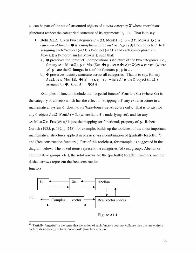
• Defn A1.2. Given two categories C = ⟨Ω, MOR(Ω),° ⟩, D = ⟨Ω’, MOR(Ω’),• ⟩, a

categorical functor ΦΦΦΦ is a morphism in the meta-category ΧΧΧΧ from objects C to D

assigning each C-object (in Ω) a D-object (in Ω’) and each C-morphism (in

MOR(Ω)) a D-morphism (in MOR(Ω’)) such that:

a.) ΦΦΦΦ preserves the ‘product’ (compositional) structure of the two categories, i.e.,

for any ϕ ∈ MOR(Ω), ψ ∈ MOR(Ω): ΦΦΦΦ(ϕ ° ψ) = ΦΦΦΦ(ϕ ) • ΦΦΦΦ(ψ) ≡ ϕ’ •ψ’ (where

ϕ’ ,ψ’ are the ΦΦΦΦ-images in D of the functors ϕ , ψ in C.

b.) ΦΦΦΦ preserves identity structure across all categories. That is to say, for any

A∈Ω, ιA ∈ MOR(Ω), ΦΦΦΦ(ιA) = ι ΦΦΦΦ(A) = ι A’ where A’ is the D-object (in Ω’)

assigned by ΦΦΦΦ. (I.e., A’ = ΦΦΦΦ(A))

Examples of functors include the ‘forgetful functor’ FOR: C→SET (where SET is

the category of all sets) which has the effect of ‘stripping off’ any extra structure in a

mathematical system C down to its ‘bare-bones’ set-structure only. That is to say, for

any C-object A∈Ω, FOR(A) = SA (where SA is A’s underlying set), and for any

ψ∈MOR(Ω): FOR(ψ) = f is just the mapping (or functional) property of ψ. Robert

Geroch (1985, p. 132, p. 248), for example, builds up the toolchest of the most important

mathematical structures applied in physics, via a combination of (partially forgetful42

)

and (free construction functors.) Part of this toolchest, for example, is suggested in the

diagram below. The boxed items represent the categories (of sets, groups, Abelian or

commutative groups, etc.), the solid arrows are the (partially) forgetful functors, and the

dashed arrows represent the free construction

functors.

etc..

Figure A1.1

42

‘Partially forgetful’ in the sense that the action of such functors does not collapse the structure entirely

back to its set-base, just to the ‘nearmost’ (simpler) structure.

SET GRP Abelian

(commutative)

Real vector spaces Complex vector

spaces

31

A.2 Clifford Algebras and Other Algebraic Structures

I proceed here by simply defining the necessary algebraic structures in an

increasing hierarchy of complexity:

Defn A2.1: (Group) A group ⟨G, °⟩ is a set G with a binary operation ° on G such

that:

a.) ° is closed with respect to G, i.e.: ∀(x, y) ∈G : (x ° y ) ≡ z ∈ G (i.e., ° is a

mapping into G or ° : G × G → G, or °(G × G) ⊆ G)).

b.) ° is associative with respect to G,: ∀(x, y, z) ∈G: (x ° y ) ° z = x ° (y ° z) ≡ x ° y °

z,

c.) There (uniquely) exists a (left/right) identity element e ∈ G : ∀ (x∈ G) ∃! (e

∈ G) : x°e = x = e°x.

d.) For every x there exists an inverse element of x, i.e.: ∀ (x∈ G) ∃ (x/ ∈ G): x° x

/

= e = x/ °x.

In terms of categories, Defn A2.1 is coextensive with that of a monoid endowed with

property A.2.1.d.). A monoid is a category in which all of its left and right identities

coincide to one unique element. For example, the integers Z form a monoid under

integer multiplication (since, ∀n∈ Z ∃! 1∈ Z such that n.1 = n = 1

.n), but not a group,

since their multiplicative inverse can violate closure. Whereas, the non-zero rational

numbers Q* =n/m | n ≠ 0, m ≠ 0 form an Abelian (i.e. commutative) group under

multiplication.

Defn A2.2: (Subgroups, Normal Subgroups, Simple Groups)

i.) Let ⟨G, °⟩ be a group. Then, for any H ⊆ G, H is a subgroup of G

(denoted: H ∠ G) if for any x, y ∈ H, then x°y /∈ H. In other words, H is

closed under °, e∈ H, and if x ∈ H then x /∈ H. If H ∠ G, and H⊂ G, then

H is a proper subgroup, denoted: H ∠ G. Moreover, if denoted: ∅⊂ H,

then H is non-trivial.

ii.) H is a normal (or invariant) subgroup of G (denoted: GH < ) if its left and

right cosets agree, for any g∈ G. That is to say, GH < iff ∀ g∈ G:

gH = gh| h∈ H= Hg = kg| k∈ H.

iii.) G is simple if G contains no proper, non-trivial, normal subgroups.

Defn A2.3: (Vector Space) A vector space is to a structure ⟨V, F, * , ⋅ ⟩ endowed with

a (commutative) operation (i.e. ∀(x,y)∈ V : x*y = y*x, denoted, by convention, by the

“+” symbol, though not necessarily to be understood as addition on the real numbers)

such that:

i) ⟨V, *⟩ is a commutative (or Abelian) group.

32

ii) Given a field43

of scalars F the scalar multiplication mapping into V ⋅ : F × V

→ V obeys distributivity (in the following two senses):

iii) ∀(α,β) ∈F ∀ ϕ ∈ V : (α +β)⋅ϕ = (α⋅ϕ) + (α⋅ϕ)

iv) ∀(ϕ , φ) ∈ V ∀γ ∈F : γ ⋅ (ϕ + φ) = (γ ⋅ϕ) + (γ ⋅ φ).

Defn A2.4: (Algebra) An algebra Α, then, is defined as a vector space ⟨V, F, * , ⋅,• ⟩ endowed with an associative binary mapping • into Α (i.e., • : Α× Α→ Α, such that

∀(ψ, ϕ, φ) ∈G: (ψ • ϕ) • φ =ψ •( ϕ • φ) ≡ ψ • ϕ •φ denoted, by convention, by the

“×” symbol, though not necessarily to be understood as ordinary multiplication on the

real numbers) This can be re-stated by saying that ⟨Α, •⟩ forms a semigroup (i.e. a

set Α closed under the binary associative product •), while ⟨Α, *⟩ forms an Abelian

group.

Examples of algebras include the class of Lie algebras, i.e. an algebra dA whose

‘product’ • is defined by an (associative) Lie product (denoted [ , ] )obeying the Jacobi

Identity: ∀(ς,ξ,ζ)∈ dA : [[ς,ξ],ζ] + [[ξ,ζ],ς] + [[ζ,ς],ξ] = 0. The structure of classes of

infinitesimal generators in many applications often form a Lie algebra. Lie algebras, in

addition, are often characterized by the behavior of their structure constants C. For any

elements of a Lie algebra ςµ ,ξν characterized by their covariant (or contravariant –if

placed above) indices (µ ,ν), then a structure constant is the indicial function C(λ)σ

µν

such that, for any ζρ ∈dA : [ ] ( ) σσ

µνσ

νµ ζλξς ∑=

=N

C1

, , where N is the dimension of dA, and

λ is the Lie Algebra’s contraction parameter. A Lie algebra is stable whenever:

limλ→∞∨λ→0 C(λ)σ

µν is well-defined for any structure constant C(λ)σ

µν and contraction

parameter λ.

Defn A2.5: (Clifford Algebra) . A Clifford Algebra is a graded algebra endowed

with the (non-commutative) Clifford product. That is to say:

i.) For any two elements A, B in a Clifford algebra CL, their Clifford product is

defined by: AB = A•B + A∧B, where A•B is their (commutative and

associative) inner product, and A∧B is their anti-commutative, i.e. A∧B = -

B∧A, and associative exterior (or Grassmann) product. This naturally makes

the Clifford product associative: A(BC) = (AB)C ≡ ABC. Less obviously,

however, for reasons that will be discussed below, is how the existence of an

43

I.e. a an algebraic structure ⟨ F, + , × ⟩ endowed with two binary operations such that ⟨F, +⟩ and ⟨F, ×⟩ form commutative groups and + , × are connected by left (and right, because of commutativity)

distributivity, i.e., ∀(α,β,γ) ∈F : α ×(β + γ) = (α ×β) + (α ×γ).

33

inverse A-1

for every (nonzero) Clifford element A arises from the Clifford

product, i.e.: A-1

A = I = AA-1

, where I is the unit pseudoscalar of CL.

ii.) CL is equipped with an adjoint ↑ and grade operator < >r (where < >r is

defined as isolating the rth grade of a Clifford element A) such that, for any

Clifford elements A, B: <AB >↑

r = (-1)C(r,2)

<B↑A

↑ >r (where: C(r ,2) =

r!/(2!(r – 2)!) =

r(r – 1)/2. )

Hence a general Clifford element (or multivector) A of Clifford algebra CL of

maximal grade N = dimV (i.e the dimension of the underlying vector space structure of

the Clifford algebra) is expressed by the linear combination:

A = α(0)A0 + α(1)

A1 + α(2)A2+ … + α(N)

AN (A.3.1)

where: α(k) | 1 ≤ k ≤ N are the elements of the scalar field (expansion coefficients)

while Ak | 1 ≤ k ≤ N are the pure Clifford elements, i.e. <Ak>l = Ak whenever k = l,

and <Ak>l = 0 otherwise, while for a general multivector (A.3.1), <A>l = α(l)Al , for

1 ≤ l ≤ N

Hence, the pure Clifford elements live in their associated closed Clifford subspaces CL(k)

of grade k, i.e. CL = CL(0) ⊕ CL(1) ⊕…⊕CL(N) .

Consider the following example: Let V = R3, i.e. the underlying vector space for

CL is a 3 dimensional Euclidean space R3

= =rr

(x,y,z) | x∈ R, y∈ R, z∈ R. Then the

maximum grade for Clifford Algebra over R3 , i.e. CL(R

3) is N = dimR

3 = 3. Hence:

CL(R3) = CL(0) ⊕ CL(1) ⊕ CL(2) ⊕CL(3) where: CL(0) (the Clifford subspace of grade 0)

is (algebraically) isomorphic to the real numbers R.44

CL(1) (the Clifford subspace of

grade 1) is algebraically isomorphic to the Complex numbers C. CL(2) (the Clifford

subspace of grade 2) is algebraically isomorphic the Quaternions H. CL(3) (the Clifford

subspace of grade 3) is algebraically isomorphic to the Octonions O.

To understand why the Clifford algebra over R3

would invariably involve closed

subspaces with elements related to the unit imaginary i =√-1 (and some of its derivative

notions thereon, in the case of the Quaternions and Octonions) entails a closer study of

the nature of the Clifford product. Defn. A.2.4 i) deliberately leaves the Grassman

product under-specified. I now fill in the details here. First, it is important to note that ∧

is a grade-raising operation: for any pure Clifford element Ak (where k < N = dimV) and

44

Since the real numbers are a field, they’re obviously describable as an algebra, in which their underlying

‘vector space’ structure is identical to their field of scalars. In other words, scalar multiplication is the

same as the ‘vector’ product •.

34

B1 , then <AkB1> = k + 1. It is for this reason that pure Clifford elements of grade k are

often called multivectors. Conversely, the inner product • is a grade-lowering operation:

for any pure Clifford element Ak (where k < N = dimV) and B1 , then <Ak•B1> = k – 1.

(Hence the inner product is often referred to as a contraction).

The reason for the grade-raising, anti-commutative nature of the Grassman

product is historically attributed to Grassman’s geometric notions of (directed) line

segments, (rays) areas, volumes, hypervolumes, etc. For example, in the case of two

vectors BArr

, , their associated directed area segments ABBAvrrr

∧∧ , are illustrated below:

Br

Br

BArr

∧ ABrr

∧

Ar

Ar

Fig. A.2.1

The notion of directed area, volume, hypervolume segments indeed survives, to a certain

limited sense, in the vector-algebraic notion of ‘cross-product.’ For example, the

magnitude of the cross-product BArr

× is precisely the area of the parallelogram spanned

by BArr

, as depicted in Fig. A.2.1. The difference, however, lies in the fixity of grade in

the case of BArr

× , in the sense that the anti-commutativity is geometrically attributed to

the directionality of the vector BArr

× (of positive sign in the case of right-handed

coordinate system) perpendicular to the plane spanned by BArr

, . This limits the notion of

the vector cross-product, as it can only be defined for spaces of maximum dimensionality

3.45

On the other hand, the Grassmann product of multivectors interpreted as directed

areas, volumes, and hypervolumes is unrestricted by the dimensionality of the vector

space.

The connection with the algebraic behavior of i =√-1 lies in the inherently anti-

commutative aspect (i.e. the Grassmann component) of the Clifford product, as discussed

above. To see this, consider the even simpler case of V = R2

(as discussed, for example,

45

“[T]he vector algebra of Gibbs…was effectively the end of the search for a unifying mathematical

language and the beginning of a proliferation of novel algebraic systems, created as and when they were

needed; for example, spinor algebra, matrix and tensor algebra, differential forms, etc.” (Lansenby, et. al.

(2000), 21)

35

in Lasenby, et. al. (2000), 26-29). Then; N = dimR2 = 2. Moreover, R

2 = ( )21

ˆ,ˆ ee ,

where ⟨…⟩ denotes the span and ( )21ˆ,ˆ ee are the ordered pair of orthonormal vectors

(parallel, for example, to the x and y axes.) Hence: ,1ˆˆ2

2

2

1 == ee and

0ˆˆˆˆ1221 =•=• eeee . So: 121221211221

ˆˆˆˆˆˆˆˆˆˆˆˆ eeeeeeeeeeee −=∧−=∧=∧+•= . Hence:

( ) ( )( ) ( ) ( ) ( )( ) ( )( ) 1ˆˆˆˆˆˆˆˆˆˆˆˆˆˆˆˆˆˆˆˆ 2

2

2

12211221121212121

2

21 −=−=−=−=== eeeeeeeeeeeeeeeeeeee (using the

anti-commutativity and associativity of the Clifford product.) Hence, the multivector

21ˆˆ ee is algebraically isomorphic to i =√-1. Moreover, ( ) 2121

ˆˆˆˆ eeee −= and ( ) 1221ˆˆˆˆ eeee = , by

the same simple algebraic maneuvering. Geometrically, then, the multivector 21ˆˆ ee when

multiplying on the left has the effect of a clockwise π/2 –rotation. Represented then in the

matrix algebra M2(R) (the algebra of real-valued 2x2 matrices):

−≡

01

10ˆˆ

21ee , where:

≡

≡

1

0ˆ,

0

1ˆ

21 ee

Moreover, for CL(R2) the multivector 21

ˆˆ ee is the unit pseudoscalar, i.e. the

element of maximal grade. In general, for any Clifford Algebra CL(V), where dimV = N,

and V = ⟨(γ1, γ2, …, γN)⟩, where the basis elements aren’t necessarily orthonormal, the

unit pseudoscalar I of CL(V) is: I = γ1γ2… γN. In general, for grade k (where 1 ≤ k ≤ N)

the closed subspaces CL(k) of grade k in CL(V) = CL(0) ⊕ CL(1) ⊕…⊕CL(N) have

dimensionality C(N,k) = N!

/[k!(N – k)!], i.e are spanned by C(N,k) = N!

/[k!(N – k)!] multivectors of

degree k. Hence the total number of Clifford basis elements generated by the Clifford

product acting on the basis elements of the underlying vector space is: ( )∑=

=N

k

NkNC

0

,2 .

The unit pseudoscalar is therefore the (one) multivector (only one there are C(N,N) =1 of

them, modulo sign or order of mutliplication) spanning the closed Clifford subspace of

maximal grade N.

For example, in the case of CL(R3) = CL(0) ⊕ CL(1) ⊕ CL(2) ⊕CL(3) , where:

R3

= ( )321ˆ,ˆ,ˆ eee :

( ) ( ) ( ) ( ) ( ) ( ) 1233231312232110 ,,,,,,,1 eICLeeeCLeeeCLRCL ====≅=

36

(where the abbreviation ei…k = ki ee ˆ...ˆ is adopted). As demonstrated in the case of CL(R2)

the multivector, the unit psuedoscalar I should not be interpreted as a multiplicative

identity, i.e. it is certainly not the case that for any A∈ CL(V), AI = A = IA. Rather, the

unit pseudoscalar is adopted to define an element of dual grade A* : for any pure Clifford

element Ak, (where 0≤ k <N) : the grade of AI (or A*) is N- k, and vice versa. Thus an

inverse element A-1

can in principle be constructed, for every nonzero A∈ CL(V). So the

linear equation AX = B has the formal solution X = A-1

B in CL(V). “Much of the power

of geometric (Clifford) algebra lies in this property of invertibility.” (Lasenby, et. al.

(2000), 25)

VI. References:

Adamek, et. al. (1990) Abstract and Concrete Categories: The Joy of Cats, New York:

Wiley & Sons.

Batterman, Robert (2002). The Devil in the Details: Asymptotic Reasoning in

Explanation, Reduction and Emergence. New York, NY: Oxford University Press.

Batterman, Robert (2003). “Response to Belot’s ‘Whose Devil? Which Details?’”

Philosophy of Science. Forthcoming. Philosophy of Science Archives: Physics

http://philsci-archive.pitt.edu/archive/00001623/

Batterman, Robert (2003). “Intertheory Relations in Physics” Stanford Encyclopaedia of

Philosophy http://plato.stanford.edu/entries/physics-interrelate/

Batterman, Robert (2004) . “Critical Phenomena and Breaking Drops” Philosophy of

Science Archives: Physics http://philsci-archive.pitt.edu/archive/00001622/

Batterman, Robert (2005) . “’Fundamental Physics’ Molecular Dynamics versus

Hydrodynamics” Philosophy of Science Archives: Physics

http://philsci-archive.pitt.edu/archive/00000582/

Baylis, ed.(1995) Clifford (Geometric) Algebras. Birkhauser .

Belot, Gordon (2003). “Whose Devil? Which Details?” Philosophy of Science.

Forthcoming. http://philsci-archive.pitt.edu/archive/00001515/

Bishop, Robert (2004). “Patching Physics and Chemistry Together” PSA 2004

http://philsci-archive.pitt.edu/archive/00001880/

Bredon, Glen (2000) Topology and Geometry, Springer-Verlag.

37

Elze, Hans-Thomas “Fluid Dynamics of Relativistic Quantum Dust,” Journal of Physics

G 28 (2002) 22235-2239

Finkelstein, David (1996). Quantum Relativity: A Synthesis of the Ideas of Einstein and

Heisenberg. Berlin: Springer-Verlag.

Finkelstein et al., (2001) Clifford Algebra as Quantum Language, J. Math. Phys 42, 1489.

http://www.physics.gatech.edu/people/faculty/finkelstein/CliffLang2001.pdf

Finkelstein, David (2002) Post Quantum Relativity (manuscript), School of Physics,

Georgia Institute of Technology, Atlanta, Georgia.

Finkelstein, David (2004a) Finite Quantum Relativity,

URL=http://www.physics.gatech.edu/people/faculty/finkelstein/FQR02.pdf

Finkelstein et al.,(2004b) Quantum Binary Gravity

URL=http://www.physics.gatech.edu/people/faculty/finkelstein/QBGravity031215.pdf

Finkelstein and Shiri-Garakani (2004c) Finite Quantum Harmonic Oscillator

URL=http://www.physics.gatech.edu/people/faculty/finkelstein/FHO0410082.pdf

Friedman, Kenneth (1982) “Is Intertheoretic Reduction Possible?” British Journal for the

Philosophy of Science, vol. 22, no. 1 (17-40).

Geroch, Robert (1985) Mathematical Physics (Chicago Lecture Series in Physics).

Chicago: University of Chicago Press.

Green, H. S. (2000) Information Theory and Quantum Physics: Physical Foundations for

Understanding the Conscious Process, Berlin: Springer-Verlag.

Hestenes and Sobczyk (1984) Clifford Algebras to Geometric Calculus: A Unified

Language for Mathematics and Physics, (Fundamental Theories of Physics), Dordrecht:

D. Reidel.

Hestenes, David (1986). “Clifford Algebra and the Interpretation of Quantum

Mechanics,” in Chisholm, J. S. R. & Commons, A. K. (eds). Clifford Algebras and their

Applications in Mathematical Physics. Dordrecht/Boston: D. Reidel, 321-346

Inonu and Wigner (1952) “On the Contraction of Groups and their Representations.”

Proceedings of the National Academy of the Sciences 39, 510-524.

Kallfelz, William (2005a) “The Renormalization Group’s Application to Turbulence: A

Doubly-Pythagorean Analogy” (unpublished manuscript) Department of Philosophy,

University of Maryland, College Park.

38

Kallfelz, William (2005b) “Contracting Batterman’s ‘No-Man’s Land:’ Reduction

Rejoins Explanation” Philosophy of Science Archives: Physics

http://philsci-archive.pitt.edu/archive/00002402/

Lasenby, J., Lasenby, A., Doran, C. (2000) “A Unified Mathematical Language for

Physics and Engineering in the 21st Century,” Phil. Trans. R. Soc. Lond. A, 358, 21-39.

Lenhard, Johannes (2004) “Nanoscience and the Janus-Faced Character of Simulations,”

in Baird, et. al., eds. Discovering the Nanoscale. Amsterdam: IOS Press, 93-100.

Mann, Stephen & Rockwood, Alyn (2003) “Computing Singularities of 3D Vector

Fields with Geometric Algebra,” Proceedings of the Conference on Visualization ’02.

Washington DC: IEEE Computer Society, 283-290

http://www.cs.brown.edu/research/vis/docs/pdf/Mann-2002-CSO.pdf

Mikhalev &. Pilz. (2002) The Concise Handbook of Algebra. Kluwer Academic

Publishers, Dordrecht.

Scheuermann, Gerik (2000) “Topological Field Visualization with Clifford Algebra”

http://www.informatik.uni-leipzig.de/TopologicalVectorField.pdf

Segal, I. E. (1951) A Class of Operator Algebras which are Determined by Groups. Duke

Mathematical Journal 18, 221.

Snygg, John (1997). Clifford Algebra: A Computational Tool for Physicists. Oxford:

Oxford University Press.

Wilczek, Frank (1999) “Projective Statistics and Spinors in Hilbert Space” hep-

th/9806228