method 6200: field portable x-ray fluorescence spectrometry for

6200 - 1 Revision 0February 2007

METHOD 6200

FIELD PORTABLE X-RAY FLUORESCENCE SPECTROMETRY FOR THEDETERMINATION OF ELEMENTAL CONCENTRATIONS IN SOIL AND SEDIMENT

SW-846 is not intended to be an analytical training manual. Therefore, methodprocedures are written based on the assumption that they will be performed by analysts who areformally trained in at least the basic principles of chemical analysis and in the use of the subjecttechnology.

In addition, SW-846 methods, with the exception of required method use for the analysisof method-defined parameters, are intended to be guidance methods which contain generalinformation on how to perform an analytical procedure or technique which a laboratory can useas a basic starting point for generating its own detailed Standard Operating Procedure (SOP),either for its own general use or for a specific project application. The performance dataincluded in this method are for guidance purposes only, and are not intended to be and mustnot be used as absolute QC acceptance criteria for purposes of laboratory accreditation.

1.0 SCOPE AND APPLICATION

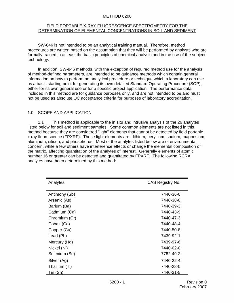
1.1 This method is applicable to the in situ and intrusive analysis of the 26 analyteslisted below for soil and sediment samples. Some common elements are not listed in thismethod because they are considered "light" elements that cannot be detected by field portablex-ray fluorescence (FPXRF). These light elements are: lithium, beryllium, sodium, magnesium,aluminum, silicon, and phosphorus. Most of the analytes listed below are of environmentalconcern, while a few others have interference effects or change the elemental composition ofthe matrix, affecting quantitation of the analytes of interest. Generally elements of atomicnumber 16 or greater can be detected and quantitated by FPXRF. The following RCRAanalytes have been determined by this method:

Analytes CAS Registry No.

Antimony (Sb) 7440-36-0Arsenic (As) 7440-38-0Barium (Ba) 7440-39-3Cadmium (Cd) 7440-43-9Chromium (Cr) 7440-47-3Cobalt (Co) 7440-48-4Copper (Cu) 7440-50-8Lead (Pb) 7439-92-1Mercury (Hg) 7439-97-6Nickel (Ni) 7440-02-0Selenium (Se) 7782-49-2Silver (Ag) 7440-22-4Thallium (Tl) 7440-28-0Tin (Sn) 7440-31-5



Vanadium (V) 7440-62-2Zinc (Zn) 7440-66-6

In addition, the following non-RCRA analytes have been determined by this method:


Calcium (Ca) 7440-70-2Iron (Fe) 7439-89-6Manganese (Mn) 7439-96-5Molybdenum (Mo) 7439-93-7Potassium (K) 7440-09-7Rubidium (Rb) 7440-17-7Strontium (Sr) 7440-24-6Thorium (Th) 7440-29-1Titanium (Ti) 7440-32-6Zirconium (Zr) 7440-67-7

1.2 This method is a screening method to be used with confirmatory analysis usingother techniques (e.g., flame atomic absorption spectrometry (FLAA), graphite furnance atomicabsorption spectrometry (GFAA), inductively coupled plasma-atomic emission spectrometry,(ICP-AES), or inductively coupled plasma-mass spectrometry, (ICP-MS)). This method’s mainstrength is that it is a rapid field screening procedure. The method's lower limits of detection aretypically above the toxicity characteristic regulatory level for most RCRA analytes. However,when the obtainable values for precision, accuracy, and laboratory-established sensitivity of thismethod meet project-specific data quality objectives (DQOs), FPXRF is a fast, powerful, costeffective technology for site characterization.

1.3 The method sensitivity or lower limit of detection depends on several factors,including the analyte of interest, the type of detector used, the type of excitation source, thestrength of the excitation source, count times used to irradiate the sample, physical matrixeffects, chemical matrix effects, and interelement spectral interferences. Example lower limitsof detection for analytes of interest in environmental applications are shown in Table 1. Theselimits apply to a clean spiked matrix of quartz sand (silicon dioxide) free of interelement spectralinterferences using long (100 -600 second) count times. These sensitivity values are given forguidance only and may not always be achievable, since they will vary depending on the samplematrix, which instrument is used, and operating conditions. A discussion of performance-basedsensitivity is presented in Sec. 9.6.

1.4 Analysts should consult the disclaimer statement at the front of the manual and theinformation in Chapter Two for guidance on the intended flexibility in the choice of methods,apparatus, materials, reagents, and supplies, and on the responsibilities of the analyst fordemonstrating that the techniques employed are appropriate for the analytes of interest, in thematrix of interest, and at the levels of concern.


In addition, analysts and data users are advised that, except where explicitly specified in aregulation, the use of SW-846 methods is not mandatory in response to Federal testingrequirements. The information contained in this method is provided by EPA as guidance to beused by the analyst and the regulated community in making judgments necessary to generateresults that meet the data quality objectives for the intended application.

1.5 Use of this method is restricted to use by, or under supervision of, personnelappropriately experienced and trained in the use and operation of an XRF instrument. Eachanalyst must demonstrate the ability to generate acceptable results with this method.

2.0 SUMMARY OF METHOD

2.1 The FPXRF technologies described in this method use either sealed radioisotopesources or x-ray tubes to irradiate samples with x-rays. When a sample is irradiated with x-rays,the source x-rays may undergo either scattering or absorption by sample atoms. This latterprocess is known as the photoelectric effect. When an atom absorbs the source x-rays, theincident radiation dislodges electrons from the innermost shells of the atom, creating vacancies. The electron vacancies are filled by electrons cascading in from outer electron shells. Electronsin outer shells have higher energy states than inner shell electrons, and the outer shell electronsgive off energy as they cascade down into the inner shell vacancies. This rearrangement ofelectrons results in emission of x-rays characteristic of the given atom. The emission of x-rays,in this manner, is termed x-ray fluorescence.

Three electron shells are generally involved in emission of x-rays during FPXRF analysisof environmental samples. The three electron shells include the K, L, and M shells. A typicalemission pattern, also called an emission spectrum, for a given metal has multiple intensitypeaks generated from the emission of K, L, or M shell electrons. The most commonlymeasured x-ray emissions are from the K and L shells; only metals with an atomic numbergreater than 57 have measurable M shell emissions.

Each characteristic x-ray line is defined with the letter K, L, or M, which signifies whichshell had the original vacancy and by a subscript alpha (α), beta (β), or gamma (γ) etc., whichindicates the higher shell from which electrons fell to fill the vacancy and produce the x-ray. Forexample, a Kα line is produced by a vacancy in the K shell filled by an L shell electron, whereasa Kβ line is produced by a vacancy in the K shell filled by an M shell electron. The Kα transitionis on average 6 to 7 times more probable than the Kβ transition; therefore, the Kα line isapproximately 7 times more intense than the Kβ line for a given element, making the Kα line thechoice for quantitation purposes.

The K lines for a given element are the most energetic lines and are the preferred lines foranalysis. For a given atom, the x-rays emitted from L transitions are always less energetic thanthose emitted from K transitions. Unlike the K lines, the main L emission lines (Lα and Lβ) for anelement are of nearly equal intensity. The choice of one or the other depends on whatinterfering element lines might be present. The L emission lines are useful for analysesinvolving elements of atomic number (Z) 58 (cerium) through 92 (uranium).

An x-ray source can excite characteristic x-rays from an element only if the source energyis greater than the absorption edge energy for the particular line group of the element, that is,the K absorption edge, L absorption edge, or M absorption edge energy. The absorption edgeenergy is somewhat greater than the corresponding line energy. Actually, the K absorptionedge energy is approximately the sum of the K, L, and M line energies of the particular element,and the L absorption edge energy is approximately the sum of the L and M line energies. FPXRF is more sensitive to an element with an absorption edge energy close to but less than


the excitation energy of the source. For example, when using a cadmium-109 source, whichhas an excitation energy of 22.1 kiloelectron volts (keV), FPXRF would exhibit better sensitivityfor zirconium which has a K line energy of 15.77 keV than to chromium, which has a K lineenergy of 5.41 keV.

2.2 Under this method, inorganic analytes of interest are identified and quantitatedusing a field portable energy-dispersive x-ray fluorescence spectrometer. Radiation from one ormore radioisotope sources or an electrically excited x-ray tube is used to generate characteristicx-ray emissions from elements in a sample. Up to three sources may be used to irradiate asample. Each source emits a specific set of primary x-rays that excite a corresponding range ofelements in a sample. When more than one source can excite the element of interest, thesource is selected according to its excitation efficiency for the element of interest.

For measurement, the sample is positioned in front of the probe window. This can bedone in two manners using FPXRF instruments, specifically, in situ or intrusive. If operated inthe in situ mode, the probe window is placed in direct contact with the soil surface to beanalyzed. When an FPXRF instrument is operated in the intrusive mode, a soil or sedimentsample must be collected, prepared, and placed in a sample cup. The sample cup is thenplaced on top of the window inside a protective cover for analysis.

Sample analysis is then initiated by exposing the sample to primary radiation from thesource. Fluorescent and backscattered x-rays from the sample enter through the detectorwindow and are converted into electric pulses in the detector. The detector in FPXRFinstruments is usually either a solid-state detector or a gas-filled proportional counter. Withinthe detector, energies of the characteristic x-rays are converted into a train of electric pulses,the amplitudes of which are linearly proportional to the energy of the x-rays. An electronicmultichannel analyzer (MCA) measures the pulse amplitudes, which is the basis of qualitative x-ray analysis. The number of counts at a given energy per unit of time is representative of theelement concentration in a sample and is the basis for quantitative analysis. Most FPXRFinstruments are menu-driven from software built into the units or from personal computers (PC).

The measurement time of each source is user-selectable. Shorter source measurementtimes (30 seconds) are generally used for initial screening and hot spot delineation, and longermeasurement times (up to 300 seconds) are typically used to meet higher precision andaccuracy requirements.

FPXRF instruments can be calibrated using the following methods: internally usingfundamental parameters determined by the manufacturer, empirically based on site-specificcalibration standards (SSCS), or based on Compton peak ratios. The Compton peak isproduced by backscattering of the source radiation. Some FPXRF instruments can becalibrated using multiple methods.

3.0 DEFINITIONS

3.1 FPXRF -- Field portable x-ray fluorescence.

3.2 MCA -- Multichannel analyzer for measuring pulse amplitude.

3.3 SSCS -- Site-specific calibration standards.

3.4 FP -- Fundamental parameter.

3.5 ROI -- Region of interest.


3.6 SRM -- Standard reference material; a standard containing certified amounts ofmetals in soil or sediment.

3.7 eV -- Electron volt; a unit of energy equivalent to the amount of energy gained byan electron passing through a potential difference of one volt.

3.8 Refer to Chapter One, Chapter Three, and the manufacturer's instructions for otherdefinitions that may be relevant to this procedure.

4.0 INTERFERENCES

4.1 The total method error for FPXRF analysis is defined as the square root of the sumof squares of both instrument precision and user- or application-related error. Generally,instrument precision is the least significant source of error in FPXRF analysis. User- orapplication-related error is generally more significant and varies with each site and methodused. Some sources of interference can be minimized or controlled by the instrument operator,but others cannot. Common sources of user- or application-related error are discussed below.

4.2 Physical matrix effects result from variations in the physical character of thesample. These variations may include such parameters as particle size, uniformity,homogeneity, and surface condition. For example, if any analyte exists in the form of very fineparticles in a coarser-grained matrix, the analyte’s concentration measured by the FPXRF willvary depending on how fine particles are distributed within the coarser-grained matrix. If thefine particles "settle" to the bottom of the sample cup (i.e., against the cup window), the analyteconcentration measurement will be higher than if the fine particles are not mixed in well and stayon top of the coarser-grained particles in the sample cup. One way to reduce such error is togrind and sieve all soil samples to a uniform particle size thus reducing sample-to-sampleparticle size variability. Homogeneity is always a concern when dealing with soil samples. Every effort should be made to thoroughly mix and homogenize soil samples before analysis. Field studies have shown heterogeneity of the sample generally has the largest impact oncomparability with confirmatory samples.

4.3 Moisture content may affect the accuracy of analysis of soil and sediment sampleanalyses. When the moisture content is between 5 and 20 percent, the overall error frommoisture may be minimal. However, moisture content may be a major source of error whenanalyzing samples of surface soil or sediment that are saturated with water. This error can beminimized by drying the samples in a convection or toaster oven. Microwave drying is notrecommended because field studies have shown that microwave drying can increase variabilitybetween FPXRF data and confirmatory analysis and because metal fragments in the samplecan cause arcing to occur in a microwave.

4.4 Inconsistent positioning of samples in front of the probe window is a potentialsource of error because the x-ray signal decreases as the distance from the radioactive sourceincreases. This error is minimized by maintaining the same distance between the window andeach sample. For the best results, the window of the probe should be in direct contact with thesample, which means that the sample should be flat and smooth to provide a good contactsurface.


4.5 Chemical matrix effects result from differences in the concentrations of interferingelements. These effects occur as either spectral interferences (peak overlaps) or as x-rayabsorption and enhancement phenomena. Both effects are common in soils contaminated withheavy metals. As examples of absorption and enhancement effects; iron (Fe) tends to absorbcopper (Cu) x-rays, reducing the intensity of the Cu measured by the detector, while chromium(Cr) will be enhanced at the expense of Fe because the absorption edge of Cr is slightly lowerin energy than the fluorescent peak of iron. The effects can be corrected mathematicallythrough the use of fundamental parameter (FP) coefficients. The effects also can becompensated for using SSCS, which contain all the elements present on site that can interferewith one another.

4.6 When present in a sample, certain x-ray lines from different elements can be veryclose in energy and, therefore, can cause interference by producing a severely overlappedspectrum. The degree to which a detector can resolve the two different peaks depends on theenergy resolution of the detector. If the energy difference between the two peaks in electronvolts is less than the resolution of the detector in electron volts, then the detector will not be ableto fully resolve the peaks.

The most common spectrum overlaps involve the Kβ line of element Z-1 with the Kα line ofelement Z. This is called the Kα/Kβ interference. Because the Kα:Kβ intensity ratio for a givenelement usually is about 7:1, the interfering element, Z-1, must be present at largeconcentrations to cause a problem. Two examples of this type of spectral interference involvethe presence of large concentrations of vanadium (V) when attempting to measure Cr or thepresence of large concentrations of Fe when attempting to measure cobalt (Co). The V Kα andKβ energies are 4.95 and 5.43 keV, respectively, and the Cr Kα energy is 5.41 keV. The Fe Kαand Kβ energies are 6.40 and 7.06 keV, respectively, and the Co Kα energy is 6.92 keV. Thedifference between the V Kβ and Cr Kα energies is 20 eV, and the difference between the Fe Kβand the Co Kα energies is 140 eV. The resolution of the highest-resolution detectors in FPXRFinstruments is 170 eV. Therefore, large amounts of V and Fe will interfere with quantitation ofCr or Co, respectively. The presence of Fe is a frequent problem because it is often found insoils at tens of thousands of parts per million (ppm).

4.7 Other interferences can arise from K/L, K/M, and L/M line overlaps, although theseoverlaps are less common. Examples of such overlap involve arsenic (As) Kα/lead (Pb) Lα andsulfur (S) Kα/Pb Mα. In the As/Pb case, Pb can be measured from the Pb Lβ line, and As can bemeasured from either the As Kα or the As Kß line; in this way the interference can be corrected. If the As Kβ line is used, sensitivity will be decreased by a factor of two to five times because it isa less intense line than the As Kα line. If the As Kα line is used in the presence of Pb,mathematical corrections within the instrument software can be used to subtract out the Pbinterference. However, because of the limits of mathematical corrections, As concentrationscannot be efficiently calculated for samples with Pb:As ratios of 10:1 or more. This high ratio ofPb to As may result in reporting of a "nondetect" or a "less than" value (e.g., <300 ppm) for As,regardless of the actual concentration present.

No instrument can fully compensate for this interference. It is important for an operator tounderstand this limitation of FPXRF instruments and consult with the manufacturer of theFPXRF instrument to evaluate options to minimize this limitation. The operator’s decision willbe based on action levels for metals in soil established for the site, matrix effects, capabilities ofthe instrument, data quality objectives, and the ratio of lead to arsenic known to be present atthe site. If a site is encountered that contains lead at concentrations greater than ten times theconcentration of arsenic it is advisable that all critical soil samples be sent off site forconfirmatory analysis using other techniques (e.g., flame atomic absorption spectrometry(FLAA), graphite furnance atomic absorption spectrometry (GFAA), inductively coupled plasma-


atomic emission spectrometry, (ICP-AES), or inductively coupled plasma-mass spectrometry,(ICP-MS)).

4.8 If SSCS are used to calibrate an FPXRF instrument, the samples collected must berepresentative of the site under investigation. Representative soil sampling ensures that asample or group of samples accurately reflects the concentrations of the contaminants ofconcern at a given time and location. Analytical results for representative samples reflectvariations in the presence and concentration ranges of contaminants throughout a site. Variables affecting sample representativeness include differences in soil type, contaminantconcentration variability, sample collection and preparation variability, and analytical variability,all of which should be minimized as much as possible.

4.9 Soil physical and chemical effects may be corrected using SSCS that have beenanalyzed by inductively coupled plasma (ICP) or atomic absorption (AA) methods. However, amajor source of error can be introduced if these samples are not representative of the site or ifthe analytical error is large. Another concern is the type of digestion procedure used to preparethe soil samples for the reference analysis. Analytical results for the confirmatory method willvary depending on whether a partial digestion procedure, such as Method 3050, or a totaldigestion procedure, such as Method 3052, is used. It is known that depending on the nature ofthe soil or sediment, Method 3050 will achieve differing extraction efficiencies for differentanalytes of interest. The confirmatory method should meet the project-specific data qualityobjectives (DQOs).

XRF measures the total concentration of an element; therefore, to achieve the greatestcomparability of this method with the reference method (reduced bias), a total digestionprocedure should be used for sample preparation. However, in the study used to generate theperformance data for this method (see Table 8), the confirmatory method used was Method3050, and the FPXRF data compared very well with regression correlation coefficients (r oftenexceeding 0.95, except for barium and chromium). The critical factor is that the digestionprocedure and analytical reference method used should meet the DQOs of the project andmatch the method used for confirmation analysis.

4.10 Ambient temperature changes can affect the gain of the amplifiers producinginstrument drift. Gain or drift is primarily a function of the electronics (amplifier or preamplifier)and not the detector as most instrument detectors are cooled to a constant temperature. MostFPXRF instruments have a built-in automatic gain control. If the automatic gain control isallowed to make periodic adjustments, the instrument will compensate for the influence oftemperature changes on its energy scale. If the FPXRF instrument has an automatic gaincontrol function, the operator will not have to adjust the instrument’s gain unless an errormessage appears. If an error message appears, the operator should follow the manufacturer’sprocedures for troubleshooting the problem. Often, this involves performing a new energycalibration. The performance of an energy calibration check to assess drift is a quality controlmeasure discussed in Sec. 9.2.

If the operator is instructed by the manufacturer to manually conduct a gain checkbecause of increasing or decreasing ambient temperature, it is standard to perform a gaincheck after every 10 to 20 sample measurements or once an hour whichever is more frequent. It is also suggested that a gain check be performed if the temperature fluctuates more than 10EF. The operator should follow the manufacturer’s recommendations for gain check frequency.


5.0 SAFETY

5.1 This method does not address all safety issues associated with its use. The useris responsible for maintaining a safe work environment and a current awareness file of OSHAregulations regarding the safe handling of the chemicals listed in this method. A reference fileof material safety data sheets (MSDSs) should be available to all personnel involved in theseanalyses.

NOTE: No MSDS applies directly to the radiation-producing instrument because that iscovered under the Nuclear Regulatory Commission (NRC) or applicable stateregulations.

5.2 Proper training for the safe operation of the instrument and radiation training

should be completed by the analyst prior to analysis. Radiation safety for each specificinstrument can be found in the operator’s manual. Protective shielding should never beremoved by the analyst or any personnel other than the manufacturer. The analyst should beaware of the local state and national regulations that pertain to the use of radiation-producingequipment and radioactive materials with which compliance is required. There should be aperson appointed within the organization that is solely responsible for properly instructing allpersonnel, maintaining inspection records, and monitoring x-ray equipment at regular intervals.

Licenses for radioactive materials are of two types, specifically: (1) a general licensewhich is usually initiated by the manufacturer for receiving, acquiring, owning, possessing,using, and transferring radioactive material incorporated in a device or equipment, and (2) aspecific license which is issued to named persons for the operation of radioactive instrumentsas required by local, state, or federal agencies. A copy of the radioactive material license (forspecific licenses only) and leak tests should be present with the instrument at all times andavailable to local and national authorities upon request.

X-ray tubes do not require radioactive material licenses or leak tests, but do requireapprovals and licenses which vary from state to state. In addition, fail-safe x-ray warning lightsshould be illuminated whenever an x-ray tube is energized. Provisions listed above concerningradiation safety regulations, shielding, training, and responsible personnel apply to x-ray tubesjust as to radioactive sources. In addition, a log of the times and operating conditions should bekept whenever an x-ray tube is energized. An additional hazard present with x-ray tubes is thedanger of electric shock from the high voltage supply, however, if the tube is properly positionedwithin the instrument, this is only a negligible risk. Any instrument (x-ray tube or radioisotopebased) is capable of delivering an electric shock from the basic circuitry when the system isinappropriately opened.

5.3 Radiation monitoring equipment should be used with the handling and operation ofthe instrument. The operator and the surrounding environment should be monitored continuallyfor analyst exposure to radiation. Thermal luminescent detectors (TLD) in the form of badgesand rings are used to monitor operator radiation exposure. The TLDs or badges should be wornin the area of maximum exposure. The maximum permissible whole-body dose fromoccupational exposure is 5 Roentgen Equivalent Man (REM) per year. Possible exposurepathways for radiation to enter the body are ingestion, inhaling, and absorption. The bestprecaution to prevent radiation exposure is distance and shielding.

6.0 EQUIPMENT AND SUPPLIES

The mention of trade names or commercial products in this manual is for illustrativepurposes only, and does not constitute an EPA endorsement or exclusive recommendation for


use. The products and instrument settings cited in SW-846 methods represent those productsand settings used during method development or subsequently evaluated by the Agency. Glassware, reagents, supplies, equipment, and settings other than those listed in this manualmay be employed provided that method performance appropriate for the intended applicationhas been demonstrated and documented.

6.1 FPXRF spectrometer -- An FPXRF spectrometer consists of four majorcomponents: (1) a source that provides x-rays; (2) a sample presentation device; (3) a detectorthat converts x-ray-generated photons emitted from the sample into measurable electronicsignals; and (4) a data processing unit that contains an emission or fluorescence energyanalyzer, such as an MCA, that processes the signals into an x-ray energy spectrum from whichelemental concentrations in the sample may be calculated, and a data display and storagesystem. These components and additional, optional items, are discussed below.

6.1.1 Excitation sources -- FPXRF instruments use either a sealed radioisotopesource or an x-ray tube to provide the excitation source. Many FPXRF instruments usesealed radioisotope sources to produce x-rays in order to irradiate samples. The FPXRFinstrument may contain between one and three radioisotope sources. Commonradioisotope sources used for analysis for metals in soils are iron Fe-55 (55Fe), cadmiumCd-109 (109Cd), americium Am-241 (241Am), and curium Cm-244 (244Cm). These sourcesmay be contained in a probe along with a window and the detector; the probe may beconnected to a data reduction and handling system by means of a flexible cable. Alternatively, the sources, window, and detector may be included in the same unit as thedata reduction and handling system.

The relative strength of the radioisotope sources is measured in units of millicuries(mCi). All other components of the FPXRF system being equal, the stronger the source,the greater the sensitivity and precision of a given instrument. Radioisotope sourcesundergo constant decay. In fact, it is this decay process that emits the primary x-raysused to excite samples for FPXRF analysis. The decay of radioisotopes is measured in"half-lives." The half-life of a radioisotope is defined as the length of time required toreduce the radioisotopes strength or activity by half. Developers of FPXRF technologiesrecommend source replacement at regular intervals based on the source's half-life. Thisis due to the ever increasing time required for the analysis rather than a decrease ininstrument performance. The characteristic x-rays emitted from each of the differentsources have energies capable of exciting a certain range of analytes in a sample. Table2 summarizes the characteristics of four common radioisotope sources.

X-ray tubes have higher radiation output, no intrinsic lifetime limit, produceconstant output over their lifetime, and do not have the disposal problems of radioactivesources but are just now appearing in FPXRF instruments. An electrically-excited x-raytube operates by bombarding an anode with electrons accelerated by a high voltage. Theelectrons gain an energy in electron volts equal to the accelerating voltage and can exciteatomic transitions in the anode, which then produces characteristic x-rays. Thesecharacteristic x-rays are emitted through a window which contains the vacuum necessaryfor the electron acceleration. An important difference between x-ray tubes and radioactivesources is that the electrons which bombard the anode also produce a continuum ofx-rays across a broad range of energies in addition to the characteristic x-rays. Thiscontinuum is weak compared to the characteristic x-rays but can provide substantialexcitation since it covers a broad energy range. It has the undesired property of producingbackground in the spectrum near the analyte x-ray lines when it is scattered by thesample. For this reason a filter is often used between the x-ray tube and the sample tosuppress the continuum radiation while passing the characteristic x-rays from the anode. This filter is sometimes incorporated into the window of the x-ray tube. The choice of


accelerating voltage is governed both by the anode material, since the electrons musthave sufficient energy to excite the anode, which requires a voltage greater than theabsorption edge of the anode material and by the instrument’s ability to cool the x-raytube. The anode is most efficiently excited by voltages 2 to 2.5 times the edge energy(most x-rays per unit power to the tube), although voltages as low as 1.5 times theabsorption edge energy will work. The characteristic x-rays emitted by the anode arecapable of exciting a range of elements in the sample just as with a radioactive source. Table 3 gives the recommended operating voltages and the sample elements excited forsome common anodes.

6.1.2 Sample presentation device -- FPXRF instruments can be operated in twomodes: in situ and intrusive. If operated in the in situ mode, the probe window is placedin direct contact with the soil surface to be analyzed. When an FPXRF instrument isoperated in the intrusive mode, a soil or sediment sample must be collected, prepared,and placed in a sample cup. For FPXRF instruments operated in the intrusive mode, theprobe may be rotated so that the window faces either upward or downward. A protectivesample cover is placed over the window, and the sample cup is placed on top of thewindow inside the protective sample cover for analysis.

6.1.3 Detectors -- The detectors in the FPXRF instruments can be either solid-state detectors or gas-filled, proportional counter detectors. Common solid-state detectorsinclude mercuric iodide (HgI2), silicon pin diode and lithium-drifted silicon Si(Li). The HgI2detector is operated at a moderately subambient temperature controlled by a low powerthermoelectric cooler. The silicon pin diode detector also is cooled via the thermoelectricPeltier effect. The Si(Li) detector must be cooled to at least -90 EC either with liquidnitrogen or by thermoelectric cooling via the Peltier effect. Instruments with a Si(Li)detector have an internal liquid nitrogen dewar with a capacity of 0.5 to 1.0 L. Proportionalcounter detectors are rugged and lightweight, which are important features of a fieldportable detector. However, the resolution of a proportional counter detector is not asgood as that of a solid-state detector. The energy resolution of a detector forcharacteristic x-rays is usually expressed in terms of full width at half-maximum (FWHM)height of the manganese Kα peak at 5.89 keV. The typical resolutions of the abovementioned detectors are as follows: HgI2-270 eV; silicon pin diode-250 eV; Si(Li)–170 eV;and gas-filled, proportional counter-750 eV.

During operation of a solid-state detector, an x-ray photon strikes a biased, solid-state crystal and loses energy in the crystal by producing electron-hole pairs. The electriccharge produced is collected and provides a current pulse that is directly proportional tothe energy of the x-ray photon absorbed by the crystal of the detector. A gas-filled,proportional counter detector is an ionization chamber filled with a mixture of noble andother gases. An x-ray photon entering the chamber ionizes the gas atoms. The electriccharge produced is collected and provides an electric signal that is directly proportional tothe energy of the x-ray photon absorbed by the gas in the detector.

6.1.4 Data processing units -- The key component in the data processing unit ofan FPXRF instrument is the MCA. The MCA receives pulses from the detector and sortsthem by their amplitudes (energy level). The MCA counts pulses per second to determinethe height of the peak in a spectrum, which is indicative of the target analyte'sconcentration. The spectrum of element peaks are built on the MCA. The MCAs inFPXRF instruments have from 256 to 2,048 channels. The concentrations of targetanalytes are usually shown in ppm on a liquid crystal display (LCD) in the instrument. FPXRF instruments can store both spectra and from 3,000 to 5,000 sets of numericalanalytical results. Most FPXRF instruments are menu-driven from software built into the


units or from PCs. Once the data–storage memory of an FPXRF unit is full or at any othertime, data can be downloaded by means of an RS-232 port and cable to a PC.

6.2 Spare battery and battery charger.

6.3 Polyethylene sample cups -- 31 to 40 mm in diameter with collar, or equivalent(appropriate for FPXRF instrument).

6.4 X-ray window film -- MylarTM, KaptonTM, SpectroleneTM, polypropylene, orequivalent; 2.5 to 6.0 µm thick.

6.5 Mortar and pestle -- Glass, agate, or aluminum oxide; for grinding soil andsediment samples.

6.6 Containers -- Glass or plastic to store samples.

6.7 Sieves -- 60-mesh (0.25 mm), stainless-steel, Nylon, or equivalent for preparingsoil and sediment samples.

6.8 Trowels -- For smoothing soil surfaces and collecting soil samples.

6.9 Plastic bags -- Used for collection and homogenization of soil samples.

6.10 Drying oven -- Standard convection or toaster oven, for soil and sediment samplesthat require drying.

7.0 REAGENTS AND STANDARDS

7.1 Reagent grade chemicals must be used in all tests. Unless otherwise indicated, itis intended that all reagents conform to the specifications of the Committee on AnalyticalReagents of the American Chemical Society, where such specifications are available. Othergrades may be used, provided it is first ascertained that the reagent is of sufficiently high purityto permit its use without lessening the accuracy of the determination.

7.2 Pure element standards -- Each pure, single-element standard is intended toproduce strong characteristic x-ray peaks of the element of interest only. Other elementspresent must not contribute to the fluorescence spectrum. A set of pure element standards forcommonly sought analytes is supplied by the instrument manufacturer, if designated for theinstrument; not all instruments require the pure element standards. The standards are used toset the region of interest (ROI) for each element. They also can be used as energy calibrationand resolution check samples.

7.3 Site-specific calibration standards -- Instruments that employ fundamentalparameters (FP) or similar mathematical models in minimizing matrix effects may not requireSSCS. If the FP calibration model is to be optimized or if empirical calibration is necessary,then SSCSs must be collected, prepared, and analyzed.

7.3.1 The SSCS must be representative of the matrix to be analyzed byFPXRF. These samples must be well homogenized. A minimum of 10 samples spanningthe concentration ranges of the analytes of interest and of the interfering elements mustbe obtained from the site. A sample size of 4 to 8 ounces is recommended, and standardglass sampling jars should be used.


7.3.2 Each sample should be oven-dried for 2 to 4 hr at a temperature of lessthan 150 EC. If mercury is to be analyzed, a separate sample portion should be dried atambient temperature as heating may volatilize the mercury. When the sample is dry, alllarge, organic debris and nonrepresentative material, such as twigs, leaves, roots, insects,asphalt, and rock should be removed. The sample should be homogenized (see Sec.7.3.3) and then a representative portion ground with a mortar and pestle or othermechanical means, prior to passing through a 60-mesh sieve. Only the coarse rockfraction should remain on the screen.

7.3.3 The sample should be homogenized by using a riffle splitter or by placing150 to 200 g of the dried, sieved sample on a piece of kraft or butcher paper about 1.5 by1.5 feet in size. Each corner of the paper should be lifted alternately, rolling the soil overon itself and toward the opposite corner. The soil should be rolled on itself 20 times. Approximately 5 g of the sample should then be removed and placed in a sample cup forFPXRF analysis. The rest of the prepared sample should be sent off site for ICP or AAanalysis. The method use for confirmatory analysis should meet the data qualityobjectives of the project.

7.4 Blank samples -- The blank samples should be from a "clean" quartz or silicondioxide matrix that is free of any analytes at concentrations above the established lower limit ofdetection. These samples are used to monitor for cross-contamination and laboratory-inducedcontaminants or interferences.

7.5 Standard reference materials -- Standard reference materials (SRMs) arestandards containing certified amounts of metals in soil or sediment. These standards are usedfor accuracy and performance checks of FPXRF analyses. SRMs can be obtained from theNational Institute of Standards and Technology (NIST), the U.S. Geological Survey (USGS), theCanadian National Research Council, and the national bureau of standards in foreign nations. Pertinent NIST SRMs for FPXRF analysis include 2704, Buffalo River Sediment; 2709, SanJoaquin Soil; and 2710 and 2711, Montana Soil. These SRMs contain soil or sediment fromactual sites that has been analyzed using independent inorganic analytical methods by manydifferent laboratories. When these SRMs are unavailable, alternate standards may be used(e.g., NIST 2702).

8.0 SAMPLE COLLECTION, PRESERVATION, AND STORAGE

Sample handling and preservation procedures used in FPXRF analyses should follow theguidelines in Chapter Three, "Inorganic Analytes."

9.0 QUALITY CONTROL

9.1 Follow the manufacturer’s instructions for the quality control procedures specific touse of the testing product. Refer to Chapter One for additional guidance on quality assurance(QA) and quality control (QC) protocols. Any effort involving the collection of analytical datashould include development of a structured and systematic planning document, such as aQuality Assurance Project Plan (QAPP) or a Sampling and Analysis Plan (SAP), whichtranslates project objectives and specifications into directions for those that will implement theproject and assess the results.

9.2 Energy calibration check -- To determine whether an FPXRF instrument isoperating within resolution and stability tolerances, an energy calibration check should be run. The energy calibration check determines whether the characteristic x-ray lines are shifting,


which would indicate drift within the instrument. As discussed in Sec. 4.10, this check alsoserves as a gain check in the event that ambient temperatures are fluctuating greatly (more than10 EF).

9.2.1 The energy calibration check should be run at a frequency consistent withmanufacturer’s recommendations. Generally, this would be at the beginning of eachworking day, after the batteries are changed or the instrument is shut off, at the end ofeach working day, and at any other time when the instrument operator believes that drift isoccurring during analysis. A pure element such as iron, manganese, copper, or lead isoften used for the energy calibration check. A manufacturer-recommended count time persource should be used for the check.

9.2.2 The instrument manufacturer’s manual specifies the channel orkiloelectron volt level at which a pure element peak should appear and the expectedintensity of the peak. The intensity and channel number of the pure element as measuredusing the source should be checked and compared to the manufacturer'srecommendation. If the energy calibration check does not meet the manufacturer'scriteria, then the pure element sample should be repositioned and reanalyzed. If thecriteria are still not met, then an energy calibration should be performed as described inthe manufacturer's manual. With some FPXRF instruments, once a spectrum is acquiredfrom the energy calibration check, the peak can be optimized and realigned to themanufacturer's specifications using their software.

9.3 Blank samples -- Two types of blank samples should be analyzed for FPXRFanalysis, specifically, instrument blanks and method blanks.

9.3.1 An instrument blank is used to verify that no contamination exists in thespectrometer or on the probe window. The instrument blank can be silicon dioxide, apolytetraflurorethylene (PTFE) block, a quartz block, "clean" sand, or lithium carbonate. This instrument blank should be analyzed on each working day before and after analysesare conducted and once per every twenty samples. An instrument blank should also beanalyzed whenever contamination is suspected by the analyst. The frequency of analysiswill vary with the data quality objectives of the project. A manufacturer-recommendedcount time per source should be used for the blank analysis. No element concentrationsabove the established lower limit of detection should be found in the instrument blank. Ifconcentrations exceed these limits, then the probe window and the check sample shouldbe checked for contamination. If contamination is not a problem, then the instrument mustbe "zeroed" by following the manufacturer's instructions.

9.3.2 A method blank is used to monitor for laboratory-induced contaminants orinterferences. The method blank can be "clean" silica sand or lithium carbonate thatundergoes the same preparation procedure as the samples. A method blank must beanalyzed at least daily. The frequency of analysis will depend on the data qualityobjectives of the project. If the method blank does not contain the target analyte at a levelthat interferes with the project-specific data quality objectives then the method blank wouldbe considered acceptable. In the absence of project-specific data quality objectives, if theblank is less than the lowest level of detection or less than 10% of the lowest sampleconcentration for the analyte, whichever is greater, then the method blank would beconsidered acceptable. If the method blank cannot be considered acceptable, the causeof the problem must be identified, and all samples analyzed with the method blank mustbe reanalyzed.


9.4 Calibration verification checks -- A calibration verification check sample is used tocheck the accuracy of the instrument and to assess the stability and consistency of the analysisfor the analytes of interest. A check sample should be analyzed at the beginning of eachworking day, during active sample analyses, and at the end of each working day. Thefrequency of calibration checks during active analysis will depend on the data quality objectivesof the project. The check sample should be a well characterized soil sample from the site that isrepresentative of site samples in terms of particle size and degree of homogeneity and thatcontains contaminants at concentrations near the action levels. If a site-specific sample is notavailable, then an NIST or other SRM that contains the analytes of interest can be used to verifythe accuracy of the instrument. The measured value for each target analyte should be within±20 percent (%D) of the true value for the calibration verification check to be acceptable. If ameasured value falls outside this range, then the check sample should be reanalyzed. If thevalue continues to fall outside the acceptance range, the instrument should be recalibrated, andthe batch of samples analyzed before the unacceptable calibration verification check must bereanalyzed.

9.5 Precision measurements -- The precision of the method is monitored by analyzinga sample with low, moderate, or high concentrations of target analytes. The frequency ofprecision measurements will depend on the data quality objectives for the data. A minimum ofone precision sample should be run per day. Each precision sample should be analyzed 7times in replicate. It is recommended that precision measurements be obtained for sampleswith varying concentration ranges to assess the effect of concentration on method precision. Determining method precision for analytes at concentrations near the site action levels can beextremely important if the FPXRF results are to be used in an enforcement action; therefore,selection of at least one sample with target analyte concentrations at or near the site actionlevels or levels of concern is recommended. A precision sample is analyzed by the instrumentfor the same field analysis time as used for other project samples. The relative standarddeviation (RSD) of the sample mean is used to assess method precision. For FPXRF data tobe considered adequately precise, the RSD should not be greater than 20 percent with theexception of chromium. RSD values for chromium should not be greater than 30 percent. Ifboth in situ and intrusive analytical techniques are used during the course of one day, it isrecommended that separate precision calculations be performed for each analysis type.

The equation for calculating RSD is as follows:

RSD = (SD/Mean Concentration) x 100

where:

RSD = Relative standard deviation for the precision measurement for theanalyte

SD = Standard deviation of the concentration for the analyteMean concentration = Mean concentration for the analyte

The precision or reproducibility of a measurement will improve with increasing count time,however, increasing the count time by a factor of 4 will provide only 2 times better precision, sothere is a point of diminishing return. Increasing the count time also improves the sensitivity,but decreases sample throughput.

9.6 The lower limits of detection should be established from actual measuredperformance based on spike recoveries in the matrix of concern or from acceptable methodperformance on a certified reference material of the appropriate matrix and within theappropriate calibration range for the application. This is considered the best estimate of the truemethod sensitivity as opposed to a statistical determination based on the standard deviation of


replicate analyses of a low-concentration sample. While the statistical approach demonstratesthe potential data variability for a given sample matrix at one point in time, it does not representwhat can be detected or most importantly the lowest concentration that can be calibrated. Forthis reason the sensitivity should be established as the lowest point of detection based onacceptable target analyte recovery in the desired sample matrix.

9.7 Confirmatory samples -- The comparability of the FPXRF analysis is determined bysubmitting FPXRF-analyzed samples for analysis at a laboratory. The method of confirmatoryanalysis must meet the project and XRF measurement data quality objectives. Theconfirmatory samples must be splits of the well homogenized sample material. In some casesthe prepared sample cups can be submitted. A minimum of 1 sample for each 20 FPXRF-analyzed samples should be submitted for confirmatory analysis. This frequency will depend onproject-specific data quality objectives. The confirmatory analyses can also be used to verifythe quality of the FPXRF data. The confirmatory samples should be selected from the lower,middle, and upper range of concentrations measured by the FPXRF. They should also includesamples with analyte concentrations at or near the site action levels. The results of theconfirmatory analysis and FPXRF analyses should be evaluated with a least squares linearregression analysis. If the measured concentrations span more than one order of magnitude,the data should be log-transformed to standardize variance which is proportional to themagnitude of measurement. The correlation coefficient (r) for the results should be 0.7 orgreater for the FPXRF data to be considered screening level data. If the r is 0.9 or greater andinferential statistics indicate the FPXRF data and the confirmatory data are statisticallyequivalent at a 99 percent confidence level, the data could potentially meet definitive level datacriteria.

10.0 CALIBRATION AND STANDARDIZATION

10.1 Instrument calibration -- Instrument calibration procedures vary among FPXRFinstruments. Users of this method should follow the calibration procedures outlined in theoperator's manual for each specific FPXRF instrument. Generally, however, three types ofcalibration procedures exist for FPXRF instruments, namely: FP calibration, empiricalcalibration, and the Compton peak ratio or normalization method. These three types ofcalibration are discussed below.

10.2 Fundamental parameters calibration -- FP calibration procedures are extremelyvariable. An FP calibration provides the analyst with a "standardless" calibration. Theadvantages of FP calibrations over empirical calibrations include the following:

• No previously collected site-specific samples are necessary, althoughsite-specific samples with confirmed and validated analytical results for allelements present could be used.

• Cost is reduced because fewer confirmatory laboratory results orcalibration standards are necessary.

However, the analyst should be aware of the limitations imposed on FP calibration byparticle size and matrix effects. These limitations can be minimized by adhering to thepreparation procedure described in Sec. 7.3. The two FP calibration processes discussedbelow are based on an effective energy FP routine and a back scatter with FP (BFP) routine. Each FPXRF FP calibration process is based on a different iterative algorithmic method. Thecalibration procedure for each routine is explained in detail in the manufacturer's user manualfor each FPXRF instrument; in addition, training courses are offered for each instrument.


10.2.1 Effective energy FP calibration -- The effective energy FP calibration isperformed by the manufacturer before an instrument is sent to the analyst. AlthoughSSCS can be used, the calibration relies on pure element standards or SRMs such asthose obtained from NIST for the FP calibration. The effective energy routine relies on thespectrometer response to pure elements and FP iterative algorithms to compensate forvarious matrix effects.

Alpha coefficients are calculated using a variation of the Sherman equation, whichcalculates theoretical intensities from the measurement of pure element samples. Thesecoefficients indicate the quantitative effect of each matrix element on an analyte'smeasured x-ray intensity. Next, the Lachance Traill algorithm is solved as a set ofsimultaneous equations based on the theoretical intensities. The alpha coefficients arethen downloaded into the specific instrument.

The working effective energy FP calibration curve must be verified before sampleanalysis begins on each working day, after every 20 samples are analyzed, and at the endof sampling. This verification is performed by analyzing either an NIST SRM or an SSCSthat is representative of the site-specific samples. This SRM or SSCS serves as acalibration check. A manufacturer-recommended count time per source should be usedfor the calibration check. The analyst must then adjust the y-intercept and slope of thecalibration curve to best fit the known concentrations of target analytes in the SRM orSSCS.

A percent difference (%D) is then calculated for each target analyte. The %Dshould be within ±20 percent of the certified value for each analyte. If the %D falls outsidethis acceptance range, then the calibration curve should be adjusted by varying the slopeof the line or the y-intercept value for the analyte. The SRM or SSCS is reanalyzed untilthe %D falls within ±20 percent. The group of 20 samples analyzed before an out-of-control calibration check should be reanalyzed.

The equation to calibrate %D is as follows:

%D = ((Cs - Ck) / Ck) x 100

where:

%D = Percent differenceCk = Certified concentration of standard sampleCs = Measured concentration of standard sample

10.2.2 BFP calibration -- BFP calibration relies on the ability of the liquidnitrogen-cooled, Si(Li) solid-state detector to separate the coherent (Compton) andincoherent (Rayleigh) backscatter peaks of primary radiation. These peak intensities areknown to be a function of sample composition, and the ratio of the Compton to Rayleighpeak is a function of the mass absorption of the sample. The calibration procedure isexplained in detail in the instrument manufacturer's manual. Following is a generaldescription of the BFP calibration procedure.

The concentrations of all detected and quantified elements are entered into thecomputer software system. Certified element results for an NIST SRM or confirmed andvalidated results for an SSCS can be used. In addition, the concentrations of oxygen andsilicon must be entered; these two concentrations are not found in standard metalsanalyses. The manufacturer provides silicon and oxygen concentrations for typical soiltypes. Pure element standards are then analyzed using a manufacturer-recommended


count time per source. The results are used to calculate correction factors in order toadjust for spectrum overlap of elements.

The working BFP calibration curve must be verified before sample analysis beginson each working day, after every 20 samples are analyzed, and at the end of the analysis. This verification is performed by analyzing either an NIST SRM or an SSCS that isrepresentative of the site-specific samples. This SRM or SSCS serves as a calibrationcheck. The standard sample is analyzed using a manufacturer-recommended count timeper source to check the calibration curve. The analyst must then adjust the y-interceptand slope of the calibration curve to best fit the known concentrations of target analytes inthe SRM or SSCS.

A %D is then calculated for each target analyte. The %D should fall within ±20percent of the certified value for each analyte. If the %D falls outside this acceptancerange, then the calibration curve should be adjusted by varying the slope of the line the y-intercept value for the analyte. The standard sample is reanalyzed until the %D falls within±20 percent. The group of 20 samples analyzed before an out-of-control calibration checkshould be reanalyzed.

10.3 Empirical calibration -- An empirical calibration can be performed with SSCS, site-typical standards, or standards prepared from metal oxides. A discussion of SSCS is includedin Sec. 7.3; if no previously characterized samples exist for a specific site, site-typical standardscan be used. Site-typical standards may be selected from commercially available characterizedsoils or from SSCS prepared for another site. The site-typical standards should closelyapproximate the site's soil matrix with respect to particle size distribution, mineralogy, andcontaminant analytes. If neither SSCS nor site-typical standards are available, it is possible tomake gravimetric standards by adding metal oxides to a "clean" sand or silicon dioxide matrixthat simulates soil. Metal oxides can be purchased from various chemical vendors. If standardsare made on site, a balance capable of weighing items to at least two decimal places isnecessary. Concentrated ICP or AA standard solutions can also be used to make standards. These solutions are available in concentrations of 10,000 parts per million, thus only smallvolumes have to be added to the soil.

An empirical calibration using SSCS involves analysis of SSCS by the FPXRF instrumentand by a conventional analytical method such as ICP or AA. A total acid digestion procedureshould be used by the laboratory for sample preparation. Generally, a minimum of 10 and amaximum of 30 well characterized SSCS, site-typical standards, or prepared metal oxidestandards are necessary to perform an adequate empirical calibration. The exact number ofstandards depends on the number of analytes of interest and interfering elements. Theoretically, an empirical calibration with SSCS should provide the most accurate data for asite because the calibration compensates for site-specific matrix effects.

The first step in an empirical calibration is to analyze the pure element standards for theelements of interest. This enables the instrument to set channel limits for each element forspectral deconvolution. Next the SSCS, site-typical standards, or prepared metal oxidestandards are analyzed using a count time of 200 seconds per source or a count timerecommended by the manufacturer. This will produce a spectrum and net intensity of eachanalyte in each standard. The analyte concentrations for each standard are then entered intothe instrument software; these concentrations are those obtained from the laboratory, thecertified results, or the gravimetrically determined concentrations of the prepared standards. This gives the instrument analyte values to regress against corresponding intensities during themodeling stage. The regression equation correlates the concentrations of an analyte with itsnet intensity.


The calibration equation is developed using a least squares fit regression analysis. Afterthe regression terms to be used in the equation are defined, a mathematical equation can bedeveloped to calculate the analyte concentration in an unknown sample. In some FPXRFinstruments, the software of the instrument calculates the regression equation. The softwareuses calculated intercept and slope values to form a multiterm equation. In conjunction with thesoftware in the instrument, the operator can adjust the multiterm equation to minimizeinterelement interferences and optimize the intensity calibration curve.

It is possible to define up to six linear or nonlinear terms in the regression equation. Terms can be added and deleted to optimize the equation. The goal is to produce an equationwith the smallest regression error and the highest correlation coefficient. These values areautomatically computed by the software as the regression terms are added, deleted, ormodified. It is also possible to delete data points from the regression line if these points aresignificant outliers or if they are heavily weighing the data. Once the regression equation hasbeen selected for an analyte, the equation can be entered into the software for quantitation ofanalytes in subsequent samples. For an empirical calibration to be acceptable, the regressionequation for a specific analyte should have a correlation coefficient of 0.98 or greater or meetthe DQOs of the project.

In an empirical calibration, one must apply the DQOs of the project and ascertain critical oraction levels for the analytes of interest. It is within these concentration ranges or around theseaction levels that the FPXRF instrument should be calibrated most accurately. It may not bepossible to develop a good regression equation over several orders of analyte concentration.

10.4 Compton normalization method -- The Compton normalization method is based onanalysis of a single, certified standard and normalization for the Compton peak. The Comptonpeak is produced from incoherent backscattering of x-ray radiation from the excitation sourceand is present in the spectrum of every sample. The Compton peak intensity changes withdiffering matrices. Generally, matrices dominated by lighter elements produce a largerCompton peak, and those dominated by heavier elements produce a smaller Compton peak. Normalizing to the Compton peak can reduce problems with varying matrix effects amongsamples. Compton normalization is similar to the use of internal standards in organics analysis. The Compton normalization method may not be effective when analyte concentrations exceed afew percent.

The certified standard used for this type of calibration could be an NIST SRM such as2710 or 2711. The SRM must be a matrix similar to the samples and must contain the analytesof interests at concentrations near those expected in the samples. First, a response factor hasto be determined for each analyte. This factor is calculated by dividing the net peak intensity bythe analyte concentration. The net peak intensity is gross intensity corrected for baselinereading. Concentrations of analytes in samples are then determined by multiplying the baselinecorrected analyte signal intensity by the normalization factor and by the response factor. Thenormalization factor is the quotient of the baseline corrected Compton Kα peak intensity of theSRM divided by that of the samples. Depending on the FPXRF instrument used, thesecalculations may be done manually or by the instrument software.

11.0 PROCEDURE

11.1 Operation of the various FPXRF instruments will vary according to themanufacturers' protocols. Before operating any FPXRF instrument, one should consult themanufacturer's manual. Most manufacturers recommend that their instruments be allowed towarm up for 15 to 30 minutes before analysis of samples. This will help alleviate drift or energycalibration problems later during analysis.


11.2 Each FPXRF instrument should be operated according to the manufacturer'srecommendations. There are two modes in which FPXRF instruments can be operated: in situand intrusive. The in situ mode involves analysis of an undisturbed soil sediment or sample. Intrusive analysis involves collection and preparation of a soil or sediment sample beforeanalysis. Some FPXRF instruments can operate in both modes of analysis, while others aredesigned to operate in only one mode. The two modes of analysis are discussed below.

11.3 For in situ analysis, remove any large or nonrepresentative debris from the soilsurface before analysis. This debris includes rocks, pebbles, leaves, vegetation, roots, andconcrete. Also, the soil surface must be as smooth as possible so that the probe window willhave good contact with the surface. This may require some leveling of the surface with astainless-steel trowel. During the study conducted to provide example performance data for thismethod, this modest amount of sample preparation was found to take less than 5 min persample location. The last requirement is that the soil or sediment not be saturated with water. Manufacturers state that their FPXRF instruments will perform adequately for soils with moisturecontents of 5 to 20 percent but will not perform well for saturated soils, especially if pondedwater exists on the surface. Another recommended technique for in situ analysis is to tamp thesoil to increase soil density and compactness for better repeatability and representativeness. This condition is especially important for heavy element analysis, such as barium. Source counttimes for in situ analysis usually range from 30 to 120 seconds, but source count times will varyamong instruments and depending on the desired method sensitivity. Due to theheterogeneous nature of the soil sample, in situ analysis can provide only “screening” type data.

11.4 For intrusive analysis of surface or sediment, it is recommended that a sample becollected from a 4- by 4-inch square that is 1 inch deep. This will produce a soil sample ofapproximately 375 g or 250 cm3, which is enough soil to fill an 8-ounce jar. However, the exactdimensions and sample depth should take into consideration the heterogeneous deposition ofcontaminants and will ultimately depend on the desired project-specific data quality objectives. The sample should be homogenized, dried, and ground before analysis. The sample can behomogenized before or after drying. The homogenization technique to be used after drying isdiscussed in Sec. 4.2. If the sample is homogenized before drying, it should be thoroughlymixed in a beaker or similar container, or if the sample is moist and has a high clay content, itcan be kneaded in a plastic bag. One way to monitor homogenization when the sample iskneaded in a plastic bag is to add sodium fluorescein dye to the sample. After the moist samplehas been homogenized, it is examined under an ultraviolet light to assess the distribution ofsodium fluorescein throughout the sample. If the fluorescent dye is evenly distributed in thesample, homogenization is considered complete; if the dye is not evenly distributed, mixingshould continue until the sample has been thoroughly homogenized. During the studyconducted to provide data for this method, the time necessary for homogenization procedureusing the fluorescein dye ranged from 3 to 5 min per sample. As demonstrated in Secs. 13.5and 13.7, homogenization has the greatest impact on the reduction of sampling variability. Itproduces little or no contamination. Often, the direct analysis through the plastic bag is possiblewithout the more labor intensive steps of drying, grinding, and sieving given in Secs. 11.5 and11.6. Of course, to achieve the best data quality possible all four steps should be followed.

11.5 Once the soil or sediment sample has been homogenized, it should be dried. Thiscan be accomplished with a toaster oven or convection oven. A small aliquot of the sample (20to 50 g) is placed in a suitable container for drying. The sample should be dried for 2 to 4 hr inthe convection or toaster oven at a temperature not greater than 150 EC. Samples may also beair dried under ambient temperature conditions using a 10- to 20-g portion. Regardless of whatdrying mechanism is used, the drying process is considered complete when a constant sampleweight can be obtained. Care should be taken to avoid sample cross-contamination and thesemeasures can be evaluated by including an appropriate method blank sample along with anysample preparation process.


CAUTION: Microwave drying is not a recommended procedure. Field studies have shown thatmicrowave drying can increase variability between the FPXRF data andconfirmatory analysis. High levels of metals in a sample can cause arcing in themicrowave oven, and sometimes slag forms in the sample. Microwave oven dryingcan also melt plastic containers used to hold the sample.

11.6 The homogenized dried sample material should be ground with a mortar and pestleand passed through a 60-mesh sieve to achieve a uniform particle size. Sample grindingshould continue until at least 90 percent of the original sample passes through the sieve. Thegrinding step normally takes an average of 10 min per sample. An aliquot of the sieved sampleshould then be placed in a 31.0-mm polyethylene sample cup (or equivalent) for analysis. Thesample cup should be one-half to three-quarters full at a minimum. The sample cup should becovered with a 2.5 µm Mylar (or equivalent) film for analysis. The rest of the soil sample shouldbe placed in a jar, labeled, and archived for possible confirmation analysis. All equipmentincluding the mortar, pestle, and sieves must be thoroughly cleaned so that any cross-contamination is below the established lower limit of detection of the procedure or DQOs of theanalysis. If all recommended sample preparation steps are followed, there is a high probabilitythe desired laboratory data quality may be obtained.

12.0 DATA ANALYSIS AND CALCULATIONS

Most FPXRF instruments have software capable of storing all analytical results andspectra. The results are displayed in ppm and can be downloaded to a personal computer,which can be used to provide a hard copy printout. Individual measurements that are smallerthan three times their associated SD should not be used for quantitation. See themanufacturer’s instructions regarding data analysis and calculations.

13.0 METHOD PERFORMANCE

13.1 Performance data and related information are provided in SW-846 methods only asexamples and guidance. The data do not represent required performance criteria for users ofthe methods. Instead, performance criteria should be developed on a project-specific basis,and the laboratory should establish in-house QC performance criteria for the application of thismethod. These performance data are not intended to be and must not be used as absolute QCacceptance criteria for purposes of laboratory accreditation.

13.2 The sections to follow discuss three performance evaluation factors; namely,precision, accuracy, and comparability. The example data presented in Tables 4 through 8were generated from results obtained from six FPXRF instruments (see Sec. 13.3). The soilsamples analyzed by the six FPXRF instruments were collected from two sites in the UnitedStates. The soil samples contained several of the target analytes at concentrations rangingfrom "nondetect" to tens of thousands of mg/kg. These data are provided for guidancepurposes only.

13.3 The six FPXRF instruments included the TN 9000 and TN Lead Analyzermanufactured by TN Spectrace; the X-MET 920 with a SiLi detector and X-MET 920 with a gas-filled proportional detector manufactured by Metorex, Inc.; the XL Spectrum Analyzermanufactured by Niton; and the MAP Spectrum Analyzer manufactured by Scitec. The TN 9000and TN Lead Analyzer both have a HgI2 detector. The TN 9000 utilized an Fe-55, Cd-109, andAm-241 source. The TN Lead Analyzer had only a Cd-109 source. The X-Met 920 with the SiLidetector had a Cd-109 and Am-241 source. The X-MET 920 with the gas-filled proportionaldetector had only a Cd-109 source. The XL Spectrum Analyzer utilized a silicon pin-diode


detector and a Cd-109 source. The MAP Spectrum Analyzer utilized a solid-state silicondetector and a Cd-109 source.

13.4 All example data presented in Tables 4 through 8 were generated using thefollowing calibrations and source count times. The TN 9000 and TN Lead Analyzer werecalibrated using fundamental parameters using NIST SRM 2710 as a calibration check sample. The TN 9000 was operated using 100, 60, and 60 second count times for the Cd-109, Fe-55,and Am-241 sources, respectively. The TN Lead analyzer was operated using a 60 secondcount time for the Cd-109 source. The X-MET 920 with the Si(Li) detector was calibrated usingfundamental parameters and one well characterized site-specific soil standard as a calibrationcheck. It used 140 and 100 second count times for the Cd-109 and Am-241 sources,respectively. The X-MET 920 with the gas-filled proportional detector was calibrated empiricallyusing between 10 and 20 well characterized site-specific soil standards. It used 120 secondtimes for the Cd-109 source. The XL Spectrum Analyzer utilized NIST SRM 2710 for calibrationand the Compton peak normalization procedure for quantitation based on 60 second counttimes for the Cd-109 source. The MAP Spectrum Analyzer was internally calibrated by themanufacturer. The calibration was checked using a well-characterized site-specific soilstandard. It used 240 second times for the Cd-109 source.

13.5 Precision measurements -- The example precision data are presented in Table 4. These data are provided for guidance purposes only. Each of the six FPXRF instrumentsperformed 10 replicate measurements on 12 soil samples that had analyte concentrationsranging from "nondetects" to thousands of mg/kg. Each of the 12 soil samples underwent 4different preparation techniques from in situ (no preparation) to dried and ground in a samplecup. Therefore, there were 48 precision data points for five of the instruments and 24 precisionpoints for the MAP Spectrum Analyzer. The replicate measurements were taken using thesource count times discussed at the beginning of this section.

For each detectable analyte in each precision sample a mean concentration, standarddeviation, and RSD was calculated for each analyte. The data presented in Table 4 is anaverage RSD for the precision samples that had analyte concentrations at 5 to 10 times thelower limit of detection for that analyte for each instrument. Some analytes such as mercury,selenium, silver, and thorium were not detected in any of the precision samples so theseanalytes are not listed in Table 4. Some analytes such as cadmium, nickel, and tin were onlydetected at concentrations near the lower limit of detection so that an RSD value calculated at 5to 10 times this limit was not possible.

One FPXRF instrument collected replicate measurements on an additional nine soilsamples to provide a better assessment of the effect of sample preparation on precision. Table5 shows these results. These data are provided for guidance purposes only. The additionalnine soil samples were comprised of three from each texture and had analyte concentrationsranging from near the lower limit of detection for the FPXRF analyzer to thousands of mg/kg. The FPXRF analyzer only collected replicate measurements from three of the preparationmethods; no measurements were collected from the in situ homogenized samples. The FPXRFanalyzer conducted five replicate measurements of the in situ field samples by takingmeasurements at five different points within the 4-inch by 4-inch sample square. Ten replicatemeasurements were collected for both the intrusive undried and unground and intrusive driedand ground samples contained in cups. The cups were shaken between each replicatemeasurement.

Table 5 shows that the precision dramatically improved from the in situ to the intrusivemeasurements. In general there was a slight improvement in precision when the sample wasdried and ground. Two factors caused the precision for the in situ measurements to be poorer. The major factor is soil heterogeneity. By moving the probe within the 4-inch by 4-inch square,


measurements of different soil samples were actually taking place within the square. Table 5illustrates the dominant effect of soil heterogeneity. It overwhelmed instrument precision whenthe FPXRF analyzer was used in this mode. The second factor that caused the RSD values tobe higher for the in situ measurements is the fact that only five instead of ten replicates weretaken. A lesser number of measurements caused the standard deviation to be larger which inturn elevated the RSD values.

13.6 Accuracy measurements -- Five of the FPXRF instruments (not including the MAPSpectrum Analyzer) analyzed 18 SRMs using the source count times and calibration methodsgiven at the beginning of this section. The 18 SRMs included 9 soil SRMs, 4 stream or riversediment SRMs, 2 sludge SRMs, and 3 ash SRMs. Each of the SRMs contained knownconcentrations of certain target analytes. A percent recovery was calculated for each analyte ineach SRM for each FPXRF instrument. Table 6 presents a summary of this data. With theexception of cadmium, chromium, and nickel, the values presented in Table 6 were generatedfrom the 13 soil and sediment SRMs only. The 2 sludge and 3 ash SRMs were included forcadmium, chromium, and nickel because of the low or nondetectable concentrations of thesethree analytes in the soil and sediment SRMs.

Only 12 analytes are presented in Table 6. These are the analytes that are ofenvironmental concern and provided a significant number of detections in the SRMs for anaccuracy assessment. No data is presented for the X-MET 920 with the gas-filled proportionaldetector. This FPXRF instrument was calibrated empirically using site-specific soil samples. The percent recovery values from this instrument were very sporadic and the data did not lenditself to presentation in Table 6.

Table 7 provides a more detailed summary of accuracy data for one particular FPXRFinstrument (TN 9000) for the 9 soil SRMs and 4 sediment SRMs. These data are provided forguidance purposes only. Table 7 shows the certified value, measured value, and percentrecovery for five analytes. These analytes were chosen because they are of environmentalconcern and were most prevalently certified for in the SRM and detected by the FPXRFinstrument. The first nine SRMs are soil and the last 4 SRMs are sediment. Percent recoveriesfor the four NIST SRMs were often between 90 and 110 percent for all analytes.

13.7 Comparability -- Comparability refers to the confidence with which one data set canbe compared to another. In this case, FPXRF data generated from a large study of six FPXRFinstruments was compared to SW-846 Methods 3050 and 6010 which are the standard soilextraction for metals and analysis by inductively coupled plasma. An evaluation ofcomparability was conducted by using linear regression analysis. Three factors weredetermined using the linear regression. These factors were the y-intercept, the slope of the line,and the coefficient of determination (r2).

As part of the comparability assessment, the effects of soil type and preparation methodswere studied. Three soil types (textures) and four preparation methods were examined duringthe study. The preparation methods evaluated the cumulative effect of particle size, moisture,and homogenization on comparability. Due to the large volume of data produced during thisstudy, linear regression data for six analytes from only one FPXRF instrument is presented inTable 8. Similar trends in the data were seen for all instruments. These data are provided forguidance purposes only.

Table 8 shows the regression parameters for the whole data set, broken out by soil type,and by preparation method. These data are provided for guidance purposes only. The soiltypes are as follows: soil 1--sand; soil 2--loam; and soil 3--silty clay. The preparation methodsare as follows: preparation 1--in situ in the field; preparation 2--intrusive, sample collected andhomogenized; preparation 3--intrusive, with sample in a sample cup but sample still wet and not


ground; and preparation 4–intrusive, with sample dried, ground, passed through a 40-meshsieve, and placed in sample cup.

For arsenic, copper, lead, and zinc, the comparability to the confirmatory laboratory wasexcellent with r2 values ranging from 0.80 to 0.99 for all six FPXRF instruments. The slopes ofthe regression lines for arsenic, copper, lead, and zinc, were generally between 0.90 and 1.00indicating the data would need to be corrected very little or not at all to match the confirmatorylaboratory data. The r2 values and slopes of the regression lines for barium and chromium werenot as good as for the other for analytes, indicating the data would have to be corrected tomatch the confirmatory laboratory.

Table 8 demonstrates that there was little effect of soil type on the regression parametersfor any of the six analytes. The only exceptions were for barium in soil 1 and copper in soil 3. In both of these cases, however, it is actually a concentration effect and not a soil effect causingthe poorer comparability. All barium and copper concentrations in soil 1 and 3, respectively,were less than 350 mg/kg.

Table 8 shows there was a preparation effect on the regression parameters for all sixanalytes. With the exception of chromium, the regression parameters were primarily improvedgoing from preparation 1 to preparation 2. In this step, the sample was removed from the soilsurface, all large debris was removed, and the sample was thoroughly homogenized. Theadditional two preparation methods did little to improve the regression parameters. This dataindicates that homogenization is the most critical factor when comparing the results. It isessential that the sample sent to the confirmatory laboratory match the FPXRF sample asclosely as possible.

Sec. 11.0 of this method discusses the time necessary for each of the sample preparationtechniques. Based on the data quality objectives for the project, an analyst must decide if it isworth the extra time necessary to dry and grind the sample for small improvements incomparability. Homogenization requires 3 to 5 min. Drying the sample requires one to twohours. Grinding and sieving requires another 10 to 15 min per sample. Lastly, when grindingand sieving is conducted, time has to be allotted to decontaminate the mortars, pestles, andsieves. Drying and grinding the samples and decontamination procedures will often dictate thatan extra person be on site so that the analyst can keep up with the sample collection crew. Thecost of requiring an extra person on site to prepare samples must be balanced with the gain indata quality and sample throughput.

13.8 The following documents may provide additional guidance and insight on thismethod and technique:

13.8.1 A. D. Hewitt, "Screening for Metals by X-ray FluorescenceSpectrometry/Response Factor/Compton Kα Peak Normalization Analysis," AmericanEnvironmental Laboratory, pp 24-32, 1994.

13.8.2 S. Piorek and J. R. Pasmore, "Standardless, In Situ Analysis of MetallicContaminants in the Natural Environment With a PC-Based, High Resolution Portable X-Ray Analyzer," Third International Symposium on Field Screening Methods for HazardousWaste and Toxic Chemicals, Las Vegas, Nevada, February 24-26, 1993, Vol 2, pp 1135-1151, 1993.

13.8.3 S. Shefsky, "Sample Handling Strategies for Accurate Lead-in-soilMeasurements in the Field and Laboratory," International Symposium of Field ScreeningMethods for Hazardous Waste and Toxic Chemicals, Las Vegas, NV, January 29-31,1997.


14.0 POLLUTION PREVENTION

14.1 Pollution prevention encompasses any technique that reduces or eliminates thequantity and/or toxicity of waste at the point of generation. Numerous opportunities for pollutionprevention exist in laboratory operation. The EPA has established a preferred hierarchy ofenvironmental management techniques that places pollution prevention as the managementoption of first choice. Whenever feasible, laboratory personnel should use pollution preventiontechniques to address their waste generation. When wastes cannot be feasibly reduced at thesource, the Agency recommends recycling as the next best option.

14.2 For information about pollution prevention that may be applicable to laboratoriesand research institutions consult Less is Better: Laboratory Chemical Management for WasteReduction available from the American Chemical Society's Department of GovernmentRelations and Science Policy, 1155 16th St., N.W. Washington, D.C. 20036, http://www.acs.org.

15.0 WASTE MANAGEMENT

The Environmental Protection Agency requires that laboratory waste managementpractices be conducted consistent with all applicable rules and regulations. The Agency urgeslaboratories to protect the air, water, and land by minimizing and controlling all releases fromhoods and bench operations, complying with the letter and spirit of any sewer discharge permitsand regulations, and by complying with all solid and hazardous waste regulations, particularlythe hazardous waste identification rules and land disposal restrictions. For further informationon waste management, consult The Waste Management Manual for Laboratory Personnelavailable from the American Chemical Society at the address listed in Sec. 14.2.

16.0 REFERENCES

1. Metorex, X-MET 920 User's Manual.

2. Spectrace Instruments, "Energy Dispersive X-ray Fluorescence Spectrometry: AnIntroduction," 1994.

3. TN Spectrace, Spectrace 9000 Field Portable/Benchtop XRF Training and ApplicationsManual.

4. Unpublished SITE data, received from PRC Environment Management, Inc.

17.0 TABLES, DIAGRAMS, FLOWCHARTS, AND VALIDATION DATA

The following pages contain the tables referenced by this method. A flow diagram of theprocedure follows the tables.


TABLE 1

EXAMPLE INTERFERENCE FREE LOWER LIMITS OF DETECTION

Analyte ChemicalAbstract

Series Number

Lower Limit of Detectionin Quartz Sand

(milligrams per kilogram) Antimony (Sb) 7440-36-0 40Arsenic (As) 7440-38-0 40Barium (Ba) 7440-39-3 20Cadmium (Cd) 7440-43-9 100Calcium (Ca) 7440-70-2 70Chromium (Cr) 7440-47-3 150Cobalt (Co) 7440-48-4 60Copper (Cu) 7440-50-8 50Iron (Fe) 7439-89-6 60Lead (Pb) 7439-92-1 20Manganese (Mn) 7439-96-5 70Mercury (Hg) 7439-97-6 30Molybdenum (Mo) 7439-93-7 10Nickel (Ni) 7440-02-0 50Potassium (K) 7440-09-7 200Rubidium (Rb) 7440-17-7 10Selenium (Se) 7782-49-2 40Silver (Ag) 7440-22-4 70Strontium (Sr) 7440-24-6 10Thallium (Tl) 7440-28-0 20Thorium (Th) 7440-29-1 10Tin (Sn) 7440-31-5 60Titanium (Ti) 7440-32-6 50Vanadium (V) 7440-62-2 50Zinc (Zn) 7440-66-6 50Zirconium (Zr) 7440-67-7 10

Source: Refs. 1, 2, and 3 These data are provided for guidance purposes only.


TABLE 2

SUMMARY OF RADIOISOTOPE SOURCE CHARACTERISTICS

Source Activity(mCi)

Half-Life(Years)

Excitation Energy(keV)

Elemental Analysis Range

Fe-55 20-50 2.7 5.9 Sulfur to ChromiumMolybdenum to Barium

K LinesL Lines

Cd-109 5-30 1.3 22.1 and 87.9 Calcium to RhodiumTantalum to LeadBarium to Uranium

K LinesK LinesL Lines

Am-241 5-30 432 26.4 and 59.6 Copper to ThuliumTungsten to Uranium

K LinesL Lines

Cm-244 60-100 17.8 14.2 Titanium to SeleniumLanthanum to Lead

K LinesL Lines

Source: Refs. 1, 2, and 3

TABLE 3

SUMMARY OF X-RAY TUBE SOURCE CHARACTERISTICS

AnodeMaterial

RecommendedVoltage Range

(kV)

K-alphaEmission

(keV)

Elemental Analysis Range

Cu 18-22 8.04 Potassium to CobaltSilver to Gadolinium

K LinesL Lines

Mo 40-50 17.4 Cobalt to YttriumEuropium to Radon

K LinesL Lines

Ag 50-65 22.1 Zinc to TechniciumYtterbium to Neptunium

K LinesL Lines

Source: Ref. 4

Notes: The sample elements excited are chosen by taking as the lower limit the same ratio ofexcitation line energy to element absorption edge as in Table 2 (approximately 0.45) and therequirement that the excitation line energy be above the element absorption edge as the upperlimit (L2 edges used for L lines). K-beta excitation lines were ignored.


TABLE 4

EXAMPLE PRECISION VALUES

AnalyteAverage Relative Standard Deviation for Each Instrument

at 5 to 10 Times the Lower Limit of DetectionTN

9000TN LeadAnalyzer

X-MET 920(SiLi

Detector)

X-MET 920(Gas-FilledDetector)

XLSpectrumAnalyzer

MAPSpectrumAnalyzer

Antimony 6.54 NR NR NR NR NRArsenic 5.33 4.11 3.23 1.91 12.47 6.68Barium 4.02 NR 3.31 5.91 NR NRCadmium 29.84a NR 24.80a NR NR NRCalcium 2.16 NR NR NR NR NRChromium 22.25 25.78 22.72 3.91 30.25 NRCobalt 33.90 NR NR NR NR NRCopper 7.03 9.11 8.49 9.12 12.77 14.86Iron 1.78 1.67 1.55 NR 2.30 NRLead 6.45 5.93 5.05 7.56 6.97 12.16Manganese 27.04 24.75 NR NR NR NRMolybdenum 6.95 NR NR NR 12.60 NRNickel 30.85a NR 24.92a 20.92a NA NRPotassium 3.90 NR NR NR NR NRRubidium 13.06 NR NR NR 32.69a NRStrontium 4.28 NR NR NR 8.86 NRTin 24.32a NR NR NR NR NRTitanium 4.87 NR NR NR NR NRZinc 7.27 7.48 4.26 2.28 10.95 0.83Zirconium 3.58 NR NR NR 6.49 NR

These data are provided for guidance purposes only.Source: Ref. 4a These values are biased high because the concentration of these analytes in the soil

samples was near the lower limit of detection for that particular FPXRF instrument.NR Not reported.NA Not applicable; analyte was reported but was below the established lower limit detection.


TABLE 5

EXAMPLES OF PRECISION AS AFFECTED BY SAMPLE PREPARATION

AnalyteAverage Relative Standard Deviation for Each Preparation Method

In Situ-FieldIntrusive-

Undried and UngroundIntrusive-

Dried and Ground

Antimony 30.1 15.0 14.4

Arsenic 22.5 5.36 3.76

Barium 17.3 3.38 2.90

Cadmiuma 41.2 30.8 28.3

Calcium 17.5 1.68 1.24

Chromium 17.6 28.5 21.9

Cobalt 28.4 31.1 28.4

Copper 26.4 10.2 7.90

Iron 10.3 1.67 1.57

Lead 25.1 8.55 6.03

Manganese 40.5 12.3 13.0

Mercury ND ND ND

Molybdenum 21.6 20.1 19.2

Nickela 29.8 20.4 18.2

Potassium 18.6 3.04 2.57

Rubidium 29.8 16.2 18.9

Selenium ND 20.2 19.5

Silvera 31.9 31.0 29.2

Strontium 15.2 3.38 3.98

Thallium 39.0 16.0 19.5

Thorium NR NR NR

Tin ND 14.1 15.3

Titanium 13.3 4.15 3.74

Vanadium NR NR NR

Zinc 26.6 13.3 11.1

Zirconium 20.2 5.63 5.18These data are provided for guidance purposes only.Source: Ref. 4a These values may be biased high because the concentration of these analytes in the soil

samples was near the lower limit of detection.ND Not detected.NR Not reported.


TABLE 6

EXAMPLE ACCURACY VALUES

Analyte

Instrument

TN 9000 TN Lead Analyzer X-MET 920 (SiLi Detector) XL Spectrum Analyzer

n Range of

% Rec.

Mean% Rec.

SD n Rangeof

% Rec.

Mean%

Rec.

SD n Rangeof

% Rec.

Mean%

Rec

SD n Rangeof

% Rec.

Mean%

Rec.

SD

Sb 2 100-149 124.3 NA -- -- -- -- -- -- -- -- -- -- -- --

As 5 68-115 92.8 17.3 5 44-105 83.4 23.2 4 9.7-91 47.7 39.7 5 38-535 189.8 206

Ba 9 98-198 135.3 36.9 -- -- -- -- 9 18-848 168.2 262 -- -- -- --

Cd 2 99-129 114.3 NA -- -- -- -- 6 81-202 110.5 45.7 -- -- -- --

Cr 2 99-178 138.4 NA -- -- -- -- 7 22-273 143.1 93.8 3 98-625 279.2 300

Cu 8 61-140 95.0 28.8 6 38-107 79.1 27.0 11 10-210 111.8 72.1 8 95-480 203.0 147

Fe 6 78-155 103.7 26.1 6 89-159 102.3 28.6 6 48-94 80.4 16.2 6 26-187 108.6 52.9

Pb 11 66-138 98.9 19.2 11 68-131 97.4 18.4 12 23-94 72.7 20.9 13 80-234 107.3 39.9

Mn 4 81-104 93.1 9.70 3 92-152 113.1 33.8 -- -- -- -- -- -- -- --

Ni 3 99-122 109.8 12.0 -- -- -- -- -- -- -- -- 3 57-123 87.5 33.5

Sr 8 110-178 132.6 23.8 -- -- -- -- -- -- -- -- 7 86-209 125.1 39.5

Zn 11 41-130 94.3 24.0 10 81-133 100.0 19.7 12 46-181 106.6 34.7 11 31-199 94.6 42.5Source: Ref. 4. These data are provided for guidance purposes only.n: Number of samples that contained a certified value for the analyte and produced a detectable concentration from the FPXRF instrument.SD: Standard deviation; NA: Not applicable; only two data points, therefore, a SD was not calculated.%Rec.: Percent recovery.-- No data.


TABLE 7

EXAMPLE ACCURACY FOR TN 9000a

StandardReferenceMaterial

Arsenic Barium Copper Lead Zinc

Cert.Conc.

Meas.Conc.

%Rec. Cert.Conc.

Meas.Conc.

%Rec. Cert.Conc.

Meas.Conc.

%Rec. Cert.Conc.

Meas.Conc.

%Rec. Cert.Conc.

Meas.Conc.

%Rec.

RTC CRM-021 24.8 ND NA 586 1135 193.5 4792 2908 60.7 144742 149947 103.6 546 224 40.9

RTC CRM-020 397 429 92.5 22.3 ND NA 753 583 77.4 5195 3444 66.3 3022 3916 129.6

BCR CRM 143R -- -- -- -- -- -- 131 105 80.5 180 206 114.8 1055 1043 99.0

BCR CRM 141 -- -- -- -- -- -- 32.6 ND NA 29.4 ND NA 81.3 ND NA

USGS GXR-2 25.0 ND NA 2240 2946 131.5 76.0 106 140.2 690 742 107.6 530 596 112.4

USGS GXR-6 330 294 88.9 1300 2581 198.5 66.0 ND NA 101 80.9 80.1 118 ND NA

NIST 2711 105 104 99.3 726 801 110.3 114 ND NA 1162 1172 100.9 350 333 94.9

NIST 2710 626 722 115.4 707 782 110.6 2950 2834 96.1 5532 5420 98.0 6952 6476 93.2

NIST 2709 17.7 ND NA 968 950 98.1 34.6 ND NA 18.9 ND NA 106 98.5 93.0

NIST 2704 23.4 ND NA 414 443 107.0 98.6 105 106.2 161 167 103.5 438 427 97.4

CNRC PACS-1 211 143 67.7 -- 772 NA 452 302 66.9 404 332 82.3 824 611 74.2

SARM-51 -- -- -- 335 466 139.1 268 373 139.2 5200 7199 138.4 2200 2676 121.6

SARM-52 -- -- -- 410 527 128.5 219 193 88.1 1200 1107 92.2 264 215 81.4

Source: Ref. 4. These data are provided for guidance purposes only.a All concentrations in milligrams per kilogram.%Rec.: Percent recovery; ND: Not detected; NA: Not applicable.-- No data.


TABLE 8

EXAMPLE REGRESSION PARAMETERS FOR COMPARABILITY1

Arsenic Barium Copper

n r2 Int. Slope n r2 Int. Slope n r2 Int. Slope

All Data 824 0.94 1.62 0.94 1255 0.71 60.3 0.54 984 0.93 2.19 0.93

Soil 1 368 0.96 1.41 0.95 393 0.05 42.6 0.11 385 0.94 1.26 0.99

Soil 2 453 0.94 1.51 0.96 462 0.56 30.2 0.66 463 0.92 2.09 0.95

Soil 3 — — — — 400 0.85 44.7 0.59 136 0.46 16.60 0.57

Prep 1 207 0.87 2.69 0.85 312 0.64 53.7 0.55 256 0.87 3.89 0.87

Prep 2 208 0.97 1.38 0.95 315 0.67 64.6 0.52 246 0.96 2.04 0.93

Prep 3 204 0.96 1.20 0.99 315 0.78 64.6 0.53 236 0.97 1.45 0.99

Prep 4 205 0.96 1.45 0.98 313 0.81 58.9 0.55 246 0.96 1.99 0.96

Lead Zinc Chromiumn r2 Int. Slope n r2 Int. Slope n r2 Int. Slope

All Data 1205 0.92 1.66 0.95 1103 0.89 1.86 0.95 280 0.70 64.6 0.42

Soil 1 357 0.94 1.41 0.96 329 0.93 1.78 0.93 — — — —

Soil 2 451 0.93 1.62 0.97 423 0.85 2.57 0.90 — — — —

Soil 3 397 0.90 2.40 0.90 351 0.90 1.70 0.98 186 0.66 38.9 0.50

Prep 1 305 0.80 2.88 0.86 286 0.79 3.16 0.87 105 0.80 66.1 0.43

Prep 2 298 0.97 1.41 0.96 272 0.95 1.86 0.93 77 0.51 81.3 0.36

Prep 3 302 0.98 1.26 0.99 274 0.93 1.32 1.00 49 0.73 53.7 0.45

Prep 4 300 0.96 1.38 1.00 271 0.94 1.41 1.01 49 0.75 31.6 0.56

Source: Ref. 4. These data are provided for guidance purposes only.1 Log-transformed datan: Number of data points; r2: Coefficient of determination; Int.: Y-intercept— No applicable data


METHOD 6200

FIELD PORTABLE X-RAY FLUORESCENCE SPECTROMETRY FOR THEDETERMINATION OF ELEMENTAL CONCENTRATIONS IN SOIL AND SEDIMENT

method 6200: field portable x-ray fluorescence spectrometry for

Documents