metalloid aluminum clusters with fluorine · metalloid aluminum clusters with fluorine 5. ... 16....

Calhoun: The NPS Institutional Archive

Theses and Dissertations Thesis and Dissertation Collection

2016-12

Metalloid aluminum clusters with fluorine

Lentsoane, Nape D.

Monterey, California: Naval Postgraduate School

http://hdl.handle.net/10945/51571

NAVAL POSTGRADUATE

SCHOOL MONTEREY, CALIFORNIA

THESIS

Approved for public release. Distribution is unlimited.

METALLOID ALUMINUM CLUSTERS WITH FLUORINE

by

Nape D. Lentsoane

December 2016

Thesis Advisor: Joseph Hooper Second Reader: James Luscombe

THIS PAGE INTENTIONALLY LEFT BLANK

i

REPORT DOCUMENTATION PAGE Form Approved OMB No. 0704-0188

Public reporting burden for this collection of information is estimated to average 1 hour per response, including the time for reviewing instruction, searching existing data sources, gathering and maintaining the data needed, and completing and reviewing the collection of information. Send comments regarding this burden estimate or any other aspect of this collection of information, including suggestions for reducing this burden, to Washington headquarters Services, Directorate for Information Operations and Reports, 1215 Jefferson Davis Highway, Suite 1204, Arlington, VA 22202-4302, and to the Office of Management and Budget, Paperwork Reduction Project (0704-0188) Washington DC 20503. 1. AGENCY USE ONLY(Leave blank)

2. REPORT DATEDecember 2016

3. REPORT TYPE AND DATES COVEREDMaster’s thesis

4. TITLE AND SUBTITLEMETALLOID ALUMINUM CLUSTERS WITH FLUORINE

5. FUNDING NUMBERS

6. AUTHOR(S) Nape D. Lentsoane7. PERFORMING ORGANIZATION NAME(S) AND ADDRESS(ES)

Naval Postgraduate School Monterey, CA 93943-5000

8. PERFORMINGORGANIZATION REPORT NUMBER

9. SPONSORING /MONITORING AGENCY NAME(S) ANDADDRESS(ES)

N/A

10. SPONSORING /MONITORING AGENCY REPORT NUMBER

11. SUPPLEMENTARY NOTES The views expressed in this thesis are those of the author and do notreflect the official policy or position of the Department of Defense or the U.S. Government. IRB number ____N/A____.

12a. DISTRIBUTION / AVAILABILITY STATEMENT Approved for public release. Distribution is unlimited.

12b. DISTRIBUTION CODE

13. ABSTRACT (maximum 200 words)

Metals have a very high energy density compared to explosives, but typically release this energy slowly via diffusion-limited combustion. There is recent interest in using molecular-scale metalloid clusters as a way to achieve very rapid rates of metal combustion. These clusters contain a mixture of low-valence metals as well as organic ligands. Here we investigate a prototypical aluminum metalloid cluster to determine system stability if the organic ligand contains significant amounts of fluorine. The fluorine can, in principle, oxidize the metallic elements, resulting in a system much like organic explosives where the fuel and oxidizer components are mere angstroms apart. We performed density functional theory calculations within the SIESTA code to examine the cluster binding energy and electronic structure. Partial fluorine substitution in a prototypical aluminum-cyclopentadienyl cluster results in increased binding and stability, likely due to weak non-covalent interactions between ligands. Ab initio molecular dynamics simulations confirm that the cluster is structurally stable when subjected to simulated annealing at elevated temperatures.

14. SUBJECT TERMSdensity functional theory, molecular dynamics, binding energy, siesta code, density of states, projected density of states

15. NUMBER OFPAGES

69 16. PRICE CODE

17. SECURITYCLASSIFICATION OF REPORT

Unclassified

18. SECURITYCLASSIFICATION OF THIS PAGE

Unclassified

19. SECURITYCLASSIFICATION OF ABSTRACT

Unclassified

20. LIMITATIONOF ABSTRACT

UU NSN 7540-01-280-5500 Standard Form 298 (Rev. 2-89)

Prescribed by ANSI Std. 239-18

ii


iii

Approved for public release. Distribution is unlimited.

METALLOID ALUMINUM CLUSTERS WITH FLUORINE

Nape D. Lentsoane Civilian, Armaments Corporation of South Africa (Armscor)

M.Tech., Tshwane University of Technology, 2008

Submitted in partial fulfillment of the requirements for the degree of

MASTER OF SCIENCE IN APPLIED PHYSICS

from the

NAVAL POSTGRADUATE SCHOOL December 2016

Approved by: Joseph Hooper Thesis Advisor

James Luscombe Second Reader

Kevin Smith Chair, Department of Physics

iv


v

ABSTRACT

Metals have a very high energy density compared to explosives, but

typically release this energy slowly via diffusion-limited combustion. There is

recent interest in using molecular-scale metalloid clusters as a way to achieve

very rapid rates of metal combustion. These clusters contain a mixture of low-

valence metals as well as organic ligands. Here we investigate a prototypical

aluminum metalloid cluster to determine system stability if the organic

ligand contains significant amounts of fluorine. The fluorine can, in principle,

oxidize the metallic elements, resulting in a system much like organic

explosives where the fuel and oxidizer components are mere angstroms apart.

We performed density functional theory calculations within the SIESTA code

to examine the cluster binding energy and electronic structure. Partial

fluorine substitution in a prototypical aluminum-cyclopentadienyl cluster

results in increased binding and stability, likely due to weak non-covalent

interactions between ligands. Ab initio molecular dynamics simulations

confirm that the cluster is structurally stable when subjected to simulated

annealing at elevated temperatures.

vi


vii

TABLE OF CONTENTS

I. INTRODUCTION AND LITERATURE REVIEW ........................................ 1

II. PROBLEM DEFINITION ............................................................................ 5

III. THEORY .................................................................................................... 7 A. DENSITY FUNCTIONAL THEORY ................................................. 7 B. MOLECULAR DYNAMICS ........................................................... 10

IV. SIMULATION SETUP .............................................................................. 13

V. RESULTS AND ANALYSIS ..................................................................... 21

VI. CONCLUDING REMARKS ...................................................................... 43

LIST OF REFERENCES ..................................................................................... 45

APPENDIX A. THE FDF FILE ........................................................................... 47

APPENDIX B. SLURM CODE SNIPPET ........................................................... 49

INITIAL DISTRIBUTION LIST ............................................................................ 51

viii


ix

LIST OF FIGURES

Figure 1. The simulation process .................................................................. 13

Figure 2. Single point energy profile vs. mesh cut-off. Optimal mesh cut-off found at 360 Ry. ....................................................................... 15

Figure 3. Monomer AlC10H12F3 .................................................................... 16

Figure 4. Monomer AlC10F15 ........................................................................ 16

Figure 5. Monomer AlC10H15 ........................................................................ 17

Figure 6. Tetramer Al4C40F60 ....................................................................... 17

Figure 7. Tetramer Al4C40H48F12 .................................................................. 18

Figure 8. Tetramer Al4C40H60 ....................................................................... 18

Figure 9. Atomic forces, good optimization ................................................... 22

Figure 10. Energy per relaxation step for AlC10H12F3 .................................... 22

Figure 11. Energy per relaxation step for AlC10F15......................................... 23

Figure 12. Energy per relaxation step for AlC10H15 ........................................ 23

Figure 13. Energy per relaxation step for Al4C40F60 ....................................... 24

Figure 14. Energy per relaxation step for Al4C40H48F12 ................................. 24

Figure 15. Energy per relaxation step for Al4C40H60 ...................................... 25

Figure 16. PDOS for AlC10H12F3 .................................................................... 27

Figure 17. Total DOS for AlC10H12F3 ............................................................. 27

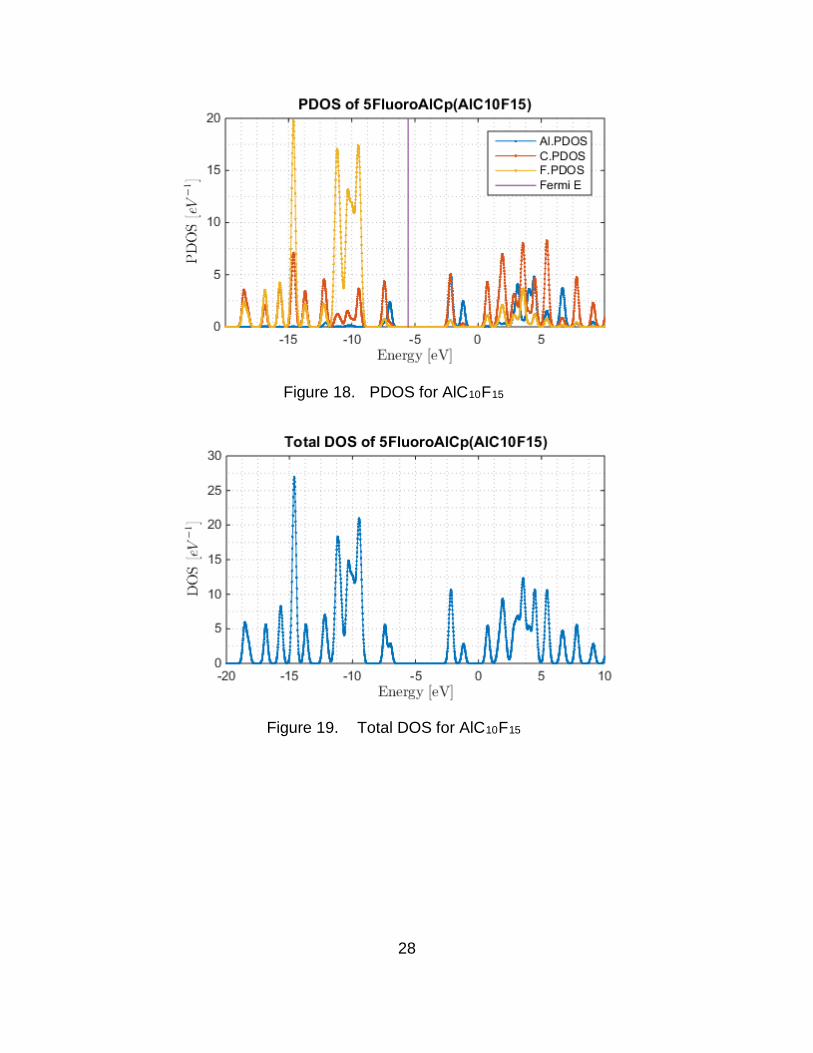
Figure 18. PDOS for AlC10F15 ........................................................................ 28

Figure 19. Total DOS for AlC10F15 .................................................................. 28

Figure 20. POS for Al4C40H60 ......................................................................... 29

Figure 21. Total DOS for Al4C40H60 ............................................................... 29

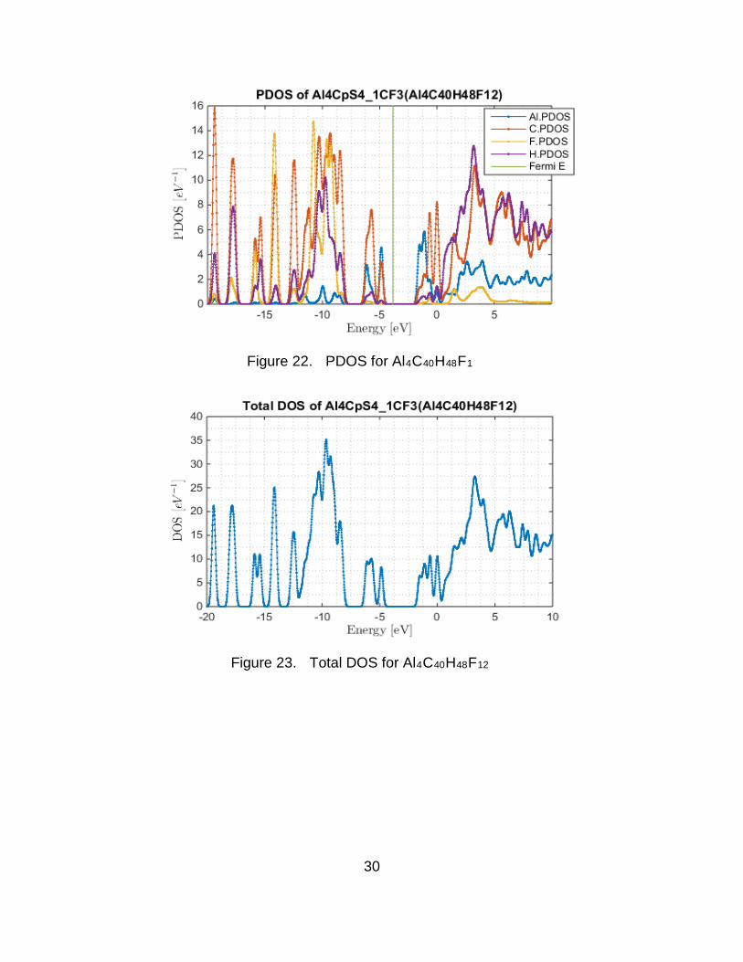
Figure 22. PDOS for Al4C40H48F1 .................................................................. 30

x

Figure 23. Total DOS for Al4C40H48F12 .......................................................... 30

Figure 24. PDOS for Al4C40H60 ...................................................................... 31

Figure 25. Total DOS for Al4C40H60 ............................................................... 31

Figure 26. PDOS for AlC10H15 ........................................................................ 32

Figure 27. Total DOS for AlC10H15 ................................................................. 32

Figure 28. Total energy drifting with MD=Verlet, and length of time step at 1 fs ................................................................................................. 33

Figure 29. Total energy conserved with MD=Verlet, and length of time step at 0.5 fs .................................................................................. 34

Figure 30. Temperature over time with Verlet and and length of time step at 1fs .............................................................................................. 34

Figure 31. Temperature over time with Verlet and length of time step at 0.5 fs .............................................................................................. 35

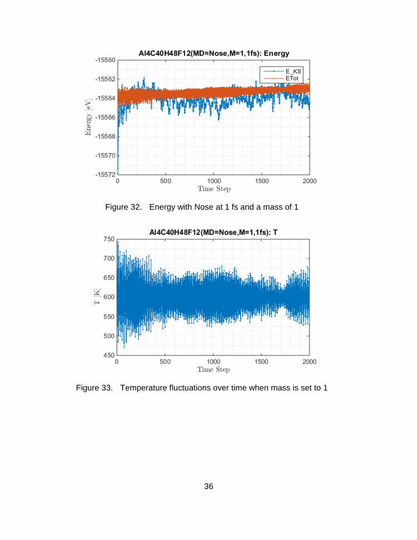
Figure 32. Energy with Nose at 1 fs and a mass of 1 ..................................... 36

Figure 33. Temperature fluctuations over time when mass is set to 1 ............ 36

Figure 34. Total energy drifting with MD=Nose, and length of time step at 1 fs and a mass of 50 .................................................................... 37

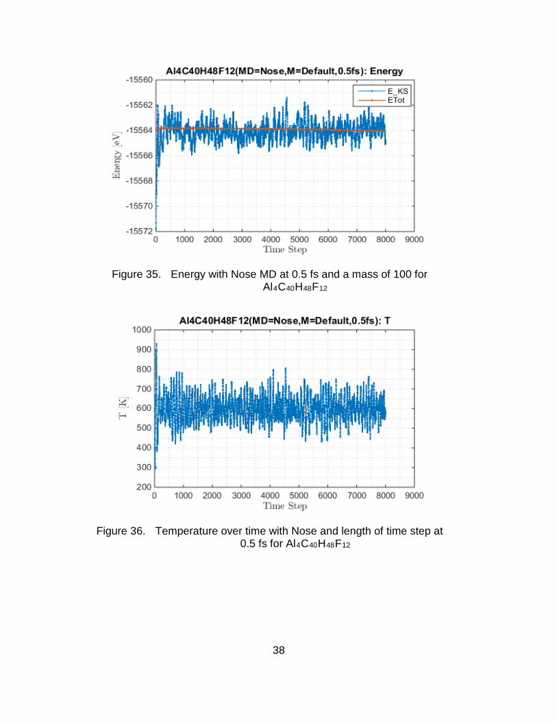
Figure 35. Energy with Nose MD at 0.5 fs and a mass of 100 for Al4C40H48F12 ................................................................................. 38

Figure 36. Temperature over time with Nose and length of time step at 0.5 fs for Al4C40H48F12 .................................................................. 38

Figure 37. Energy with Nose MD at 0.5 fs and a mass of 100 for Al4C40H60 ...................................................................................... 39

Figure 38. Temperature over time with Nose and and length of time step at 0.5 fs for Al4C40H60 ................................................................... 39

Figure 39. Snapshot of trajectory at start ........................................................ 40

Figure 40. Snapshot of trajectory after 400 time steps ................................... 41

Figure 41. Snapshot of trajectory after 5000 time steps ................................. 41

Figure 42. Snapshot of trajectory after 10566 time steps ............................... 42

xi

LIST OF TABLES

Table 1. Bond lengths in Angstroms (Å) ...................................................... 25

Table 2. Calculated binding energy, HOMO/LUMO gap and Fermi energy ........................................................................................... 33

xii


xiii

LIST OF ACRONYMS AND ABBREVIATIONS

CG Conjugate Gradient Cp Cyclopentadienyl DFT Density Functional Theory DOS Density of States fs femto-second GGA Generalized Gradient Approximation H-K Hohenberg-Kohn theorem HPC High Performance Computing K-S Kohn-Shame framework LDA Local Density Approximation MD Molecular Dynamics NVE Constant number, Volume, and Energy NVT Constant number, Volume, and Temperature Ry Rydberg

xiv


xv

ACKNOWLEDGMENTS

I would like to express my gratitude to my advisor and second reader for

their continued support. I would like to acknowledge my family for their support

and patience.

I dedicate this work to Abbaasah and my two kids, Samira and Nusaybah.

xvi


1

I. INTRODUCTION AND LITERATURE REVIEW

Metals are highly energetic materials that are commonly used to enhance

explosive formulations. Despite their high energy content, metals tend to burn

slowly through a diffusion-limited process. Recently there has been interest in

creating low-valence metal clusters which retain some of the high energy density

of bulk metals but may allow for significantly faster combustion kinetics. The core

of this research work is to study hypothetic fluorinated aluminium clusters to

determine their electronic structure and stability. The fluorine is integrated directly

into the ligands around the cluster, placing low-valence metal fuel within a few

chemical bonds of a strong oxidizer. Density functional theory as implemented in

the SIESTA code is used to study these systems, and ab initio molecular

dynamics is used as an initial check on their stability.

A number of previous works have examined aluminium-based clusters.

Mandado et al. [1] studied the properties of bonding in all-metal clusters

containing Al4 units. The Al4 was evaluated when attached to an alkaline or

transitional metals, namely Na, Li, Be, Cu and Zn. Mandado et al. [1] employed

Density Functional Theory (DFT) methods combined with the quantum theory of

atoms in molecules (QTAIM) to study the local aromaticity of Al4 fragments.

Various aluminium type clusters were evaluated by Williams and

Hooper [2]. Williams and Hooper focused their study on the structure,

thermodynamics and energies of Aluminium-Cyclopentadienyl clusters [2]. The

study used the B3LYP functional performed with the Gaussian 09 program and

compared to the G2 method. The clusters were of types Al4Cp4, Al4Cp4*, Al8Cp4,

Al8Cp4*, Al50Cp12, and Al50Cp12*. The Cp derivatives were nitro-Cp (C5H4NO2),

trifluoromethyl-Cp* (C5Me4CF3), and pentatrifluoromethyl-Cp* (C5[CF3]5) which

served as oxidizers for the aluminium complexes [2]. Williams and Hooper found

that AlCp3 and AlCp3* systems exhibited significant steric interaction between the

ligands [2]. In conclusion, Williams and Hooper suggested that thermal

decomposition in these clusters will proceed via the loss of surface metal ligand

2

units, exposing the interior aluminium core. The energy density of the large

clusters, as gauged by their volumetric heat of combustion, was calculated to be

nearly 60% that of pure aluminium [2].

In this work, we examine clusters that contain a combination of metal-

metal Al bonds as well as metal/organic bonds. These are often given the term

“metalloid” and were investigated extensively by Schnockel and collaborators [3].

We focus on a small, prototypical cluster containing four aluminium atoms, each

attached to a cyclopentadienyl (Cp) type ligand. Our particular focus is on

integration of fluorine into these ligands. Fluorine is attractive because it can

serve as a powerful oxidizer for the low-valent aluminium core in these clusters,

and its close proximity in the cluster may avoid lengthy mass diffusion processes

for fuel and oxidizer to mix. We evaluate the stability, binding energy, and

electronic structure of Cp-type ligands with either one or five methyl groups

replaced with trifluoromethyl (-CF3) groups.

For our study the focus has been restricted to analyzing the fluorinated

and non-fluorinated monomers (AlCp*) AlC10H12F3, AlC10F15, and AlC10H15 and

the fluorinated and non-fluorinated clusters (Al4Cp4*) Al4C40F60, Al4C40H48F12,

Al4C40H60. The binding energy of the tetramers is then compared to that of the

basic single aluminium with ligand molecules. For all systems geometric

optimization is performed. Our Molecular dynamics is focused on the partially-

fluorinated (Al4C40H48F12) and the fully-hydrogenated (Al4C40H60) clusters. The

fully-hydrogenated cluster has already been well characterized experimentally by

Huber and Schnöckel [3].

Wantanabe et al. [4] used DFT to study the stabilization of an Al13 cluster

with Poly(vinylpyrrolidone) (PVP). Wantanabe et al. [4] found that stabilization

was mainly due to bonding interactions between molecular orbitals of PVP and

the 1s or 1d orbitals of Al13. A study involving the binding of Aluminium to

Fluorine was undertaken by Karpukhina et al. [5]. The systems were of alkali-

fluoride types. The targeted application was heat-resistant glass ceramic. It was

found that for aluminosilicate glasses the Al-F bonding increases with

3

temperature. The reactivity of the H atom with Al13 cluster was also analyzed by

Mañanes et al. [6]. Although density functional concepts were used, Mañanes et

al. also employed Fukui analysis.

All calculations in this work are performed with the SIESTA code. SIESTA

scales very efficiently with the number of atoms and with parallel processing

power, making it a suitable choice for eventual simulations of metalloid clusters

with thousands of atoms [7]. The code uses the standard Kohn-Sham self-

consistent density functional method in the local density (LDA-LSD) and

generalized gradient (GGA) approximations, as well as in a non-local functional

that includes van der Waals interactions (VDW-DF) [8]. SIESTA uses norm-

conserving pseudopotentials that are available online from the SIESTA website.

In this work we used default pseudopotential from the SIESTA repository

at http://departments.icmab.es/leem/siesta/Databases.

The chapter outline of this report is as follows. In Chapter I current

available literature is reviewed and scope of this report given. In Chapter II the

purpose of our study is concisely defined. Chapter III presents density functional

theory, and the theory behind molecular dynamics. The Monte-Carlo runs

computed with SIESTA for molecular dynamics are performed with the Nose

method (NVT dynamics with Nose thermostat). In Chapter IV is the simulation

setup. Results and analysis follow in Chapter V and concluding remarks in

Chapter VI.

http://departments.icmab.es/leem/siesta/Databases

4


5

II. PROBLEM DEFINITION

The purpose of this thesis is to understand the aluminium based

monomers and Al4 clusters, including their stability geometry, and electronic

structure. The binding energy will be analyzed as well as the interaction between

the molecular orbitals and thus which orbitals are responsible for the binding.

Structural relaxation will be performed and final energy of the system computed.

The secondary goal is to simulate the molecular dynamics of the system

and evaluate how the system evolves with time. This is also a simple way to

roughly examine the influence of temperature on the systems. In Molecular

Dynamics simulations, one computes the evolution of the positions and velocities

with time, solving Newton’s equations. The SIESTA code contains the algorithms

to perform this. The Nose (NVT dynamics with Nose thermostat) method is used

to perform molecular dynamics.

The research question explored in this paper is: Are metalloid aluminum

clusters using fluorinated Cp ligands just as stable as those with traditional Cp?

6


7

III. THEORY

A. DENSITY FUNCTIONAL THEORY

Density functional theory has been in use for many years. The DFT is

used to study the electronic structure of many-body systems [9]. The many-body

systems investigated include atoms, molecules, and condensed phases [9]. In

principle the idea is to find the ground state of these systems. The DFT roots can

be traced as far back as the mid-1960s in the Hohenberg–Kohn theorems (H-K).

Functional simply refers to the function of a function. The challenge in this

quantum mechanical modeling method is then to find the correct ground state of

electron density that achieves energy minimization. The SIESTA code used in

this study employs the framework of Kohn-Sham DFT.

Fundamentally in DFT we solve the many-body Schrödinger equation:

, ,i I i IH r R E r R ,

where H is the Hamiltonian operator, ir and IR are a bunch of electrons and

nuclei respectively, and E is the total energy. The Hamiltonian operator is an

energy operator defined as

coulombH T V

Here, T is the kinetic energy operator, and coulombV is the coulomb potential

operator also defined as

i jcoulomb

i j

q qV

r r

The coulombV operator describes the interaction between charged particles.

The above equation involves a bunch of electrons and a bunch of nuclei which

makes solving it more complex. To remedy the complexity, the Born

8

Oppenheimer approximation is used. The Born Oppenheimer approximation

states that the mass of the nuclei is much greater than that of the electrons i.e.

nuclei em m [10]. Also the nuclei are slow whilst the electrons are fast. This implies

that we can decouple the dynamics of the nuclei and the electrons.

,i I N i e Ir R r R

This reduces the number of variables in the original equation to focus on a finite

number of electrons.

1 2 1 2, ,..., , ,...,N NH Er r r r r r

The Hamiltonian will now consist of terms dealing with electrons only,

22

1

( ) ( , )2

e e eN N N

i ext i i ji i i je

hH V r U r rm

The second term in the above equation is the potential term that

encompasses the electron-nuclei interaction. The last term is the electron-

electron interaction (i.e., repulsions). Even though the equations have been

reduced to electron terms the challenge is still to reduce the dimensionality. To

state the problem of dimensionality, for example, Al has 13 electrons and each

electron is defined by three spatial coordinates. Therefore the solving the

Schrödinger equation becomes a 39 dimensional problem ( 3 13 39 ) for a

single Al atom. Thus when forming a cluster the dimensions increase in multiples

e.g., 50 Al atoms in a cluster implies 1950 dimensional problem and a 100 atom

Au cluster is a 23700 dimensional problem.

The DFT deals with the dimensionality problem by defining the electron

density

*

1 2 1 2( ) ( , ,... ) ( , ,... )N Nn r r r r r r r

9

or, more compactly,

*( ) 2 ( ) ( )i i

i

n r r r

and therefore the dimensionality goes as 3 3N . This changes the problem to a

many one electron problem. Recall that from the H-K theorem we are trying to

find the ground state energy E . The ground state energy is said to be a unique

functional [10].

[ ( )]E E n= r

To find the ground state the energy functional is minimized by searching

for a zero gradient along the energy surface. The energy functional consists of

two parts. The part that is known involves the kinetic energy and all the potentials

aforementioned. The unknown part, exchange-correlation functional, has to be

approximated. Available in SIESTA are the Local Density Approximation (LDA)

and the Generalized Gradient Approximation (GGA). For our work we use the

GGA. In obtaining the true ground state SIESTA employs the Kohn-Sham self-

consistency scheme. The self-consistency scheme’s first step is to arbitrarily

guess the input electron density ( )n r . Thereafter solve the Kohn-Sham equations

to find a set of electron wave functions i . Re-use these wave functions to

calculate the electron density. The calculated electron density is then matched

with the input electron density. If the calculated and the input are the same then

the ground state has been found otherwise repeat the process. In SIESTA the

tolerance of this sameness can be specified.

Molecular geometry optimization. In investigating our chosen systems we

perform geometry optimization of the molecules as a first step. Geometry

optimization is a process of searching for the coordinates that minimize the total

energy of the system. The search can be stated mathematically as

10

0, ,

, , arg mini i i

i i i tx y z

x y z H

where , ,i i ix y z are the spatial positions of the atoms. Once again we look for zero

gradient of the energy

ii

EEx

Our SIESTA setup uses the conjugate gradient (CG). The CG is used to

solve the unconstrained optimization problem. The ways to verify if SIESTA has

performed the structural geometry relaxation correctly are discussed in Chapter

V (Results and Analysis). SIESTA will also churn out the atomic forces at every

relaxation step as it attempts to find the ground state.

The pseudopotential files, required at runtime, characterize the electron

density with a smoothed density. This is referred to as the frozen core

approximation [10].

B. MOLECULAR DYNAMICS

Generally, in molecular dynamics we are attempting to solve Newton’s 2nd

law for our molecular system(s). Molecular dynamics (MD) treats electrons

quantum mechanically and nuclei classically [11]. In MD we are able to

investigate the time evolution of the system. MD also allows us to evaluate the

influence of temperature on the molecular system. Thus, we gain information

about the thermal stability of our clusters.

The basic equation to be solved in MD is

2

2

( )( ) ( )dE d x tF t ma t mdtd x

11

⇒ 0 0

' '' ''0 0 0

1( ) ( ) ( )( ) ( )t t

t t

x t x t v t t t dt F t dtm

The MD simulation computes the system evolution of positions and

velocities with time [11]. The simulation obtains positions and velocities at a later

time t t . The SIESTA simulation setup allows the user to choose t referred

to as the time step. In our simulations we set time step to 1 fs (femto-second). A

smaller t∆ improves the accuracy of sampling high frequency motion. The

equations of motion are solved at each time step. MD continually takes the time

averages and statistical averages until the system reaches equilibrium. The

system is at equilibrium if the averages of the dynamical and structural quantities

remain unchanged with time.

There are various algorithms available for MD in SIESTA. For our setup

we used both the NVE (Verlet) and NVT (Nose). The Verlet employs a

microcanonical ensemble, whereby the total energy is kept constant. Therefore,

the Verlet is used to verify for correct parameterization by checking for energy

conservation violations. In the Nose (canonical ensemble) case the enforced

temperature is kept constant while changing the kinetic energy of the atoms.

12


13

IV. SIMULATION SETUP

The simulation process is simplified as having four basic attributes: the

input, simulation block, post-processing, and output. The simulation block is

where all the SIESTA algorithms are located i.e. geometry optimization and MD.

This process is depicted in Figure 1.

Figure 1. The simulation process

The simulation is performed with resources from Hamming HPC. In order

for the SIESTA jobs to run parallel on Hamming we require the Intel compiler,

OpenMPI and a compiled version of SIESTA. These packages are version

sensitive and therefore care must be ensured when working with them. A simple

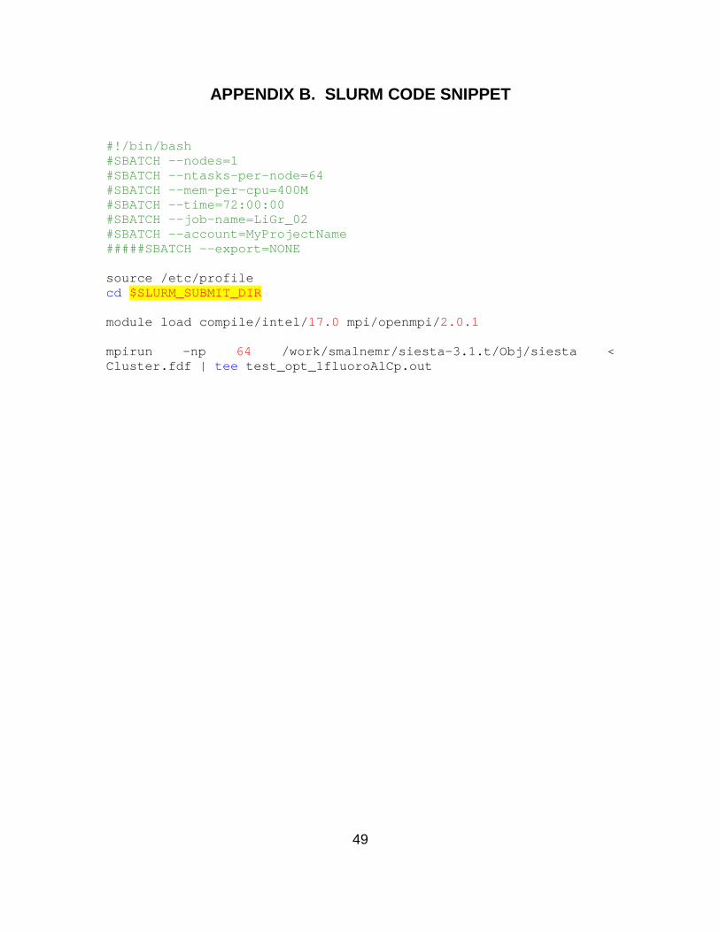
script based on SLURM was written to schedule the jobs on Hamming. The

SLURM script tells Hamming where to find the Intel compiler, OpenMPI and

SIETA executables. Also, the SLURM script specifies required memory, number

of nodes and wall time. The code snippet in Appendix B illustrates the SLURM

script.

In the snippet in Appendix B, one node with 64 tasks per node is

requested from Hamming. The memory required is 1 Gigabyte. The wall time is

set at 72 hours, which is reasonable because although the optimization takes

approximately 4 to 5 hours, the MD runs normally take 3 days or more. The Intel

compiler version 17.0 and OpenMPI version 2.0.1 were found to work well with

the SIESTA version 3.2-pl-5. Other versions are available but gave compatibility

errors. The output is redirected to the ‘*.out’ file.

For SIESTA to run correctly the input must be in the correct format. The

main input file that tells SIESTA what to do is in the Flexible Data Format (FDF)

14

with the extension ‘*.fdf’. As an example, the FDF file for the AlC10H12F3 system

is attached in Appendix A. A thorough description of the FDF file can be found in

the SIESTA manual [7]. Here we describe some of the important parameters of

our setup.

The total number of atoms in a molecule is specified. The number of atom

species contained in the molecule is also given as an input. For example, the

AlC10H12F3 has four number of atoms species. SIESTA will match the values of

these parameters with the number of positions it finds in the supplied spatial

coordinates. The coordinates are specified in angstroms.

The exchange-correlation functional is set to Generalized Gradient

Approximation (GGA, PBE version) for all systems. The basis size is set to

Double Zeta with Polarization (DZP). When performing structural relaxation, the

Conjugate Gradient (CG) minimization algorithm is used. The other important

parameter goes about how best to mesh the electron density. The mesh size,

also called the mesh cut-off energy, is chosen to be 360 Ry (Rydberg). To find

the optimal cut-off energy we compute the single point energy calculation. The

calculation is performed with different mesh sizes. The mesh size is tweaked until

the computed energy changes only by small amounts. We then plot the final

energy vs mesh to evaluate the energy profiles of the systems. Figure 2 shows

the energy profile for finding the optimal mesh cut-off. The final energy continues

to descend until it no longer has significant changes. As can be seen in the figure

the final energy difference between 350 Ry and 360 Ry is approximately 0.1

meV. Beyond this point the energy does not change significantly and therefore

360 Ry was chosen as the optimal mesh cut-off energy.

15

Figure 2. Single point energy profile vs. mesh cut-off. Optimal mesh cut-off found at 360 Ry.

Once the mesh cut-off energy has been found we are ready to perform

geometry optimization. The number of CG steps maximally allowed is 500. The

tolerance in the computed forces is set to 0.04 eV/Ang. The simulation box size

remains default. The rest of the FDF file specifies which output to write out.

The MD scheme we are mostly interested in is the NVT Nose canonical

ensemble. The NVE (Verlet) is also used but rather mainly for ensuring that

energy is properly conserved with the chosen parameters. Also, the Verlet

algorithm helps in finding the best parameter specification for the Nose. The

optimal length of a time step was found to be 0.5 fs (femto-second). The MD runs

are all performed with a temperature of 600K enforced.

The systems under investigation. The systems we investigated are 3

monomers (AlC10H12F3, AlC10F15, and AlC10H15) and 3 tetramers (Al4C40F60,

16

Al4C40H48F12, and Al4C40H60). These systems are shown in Figure 3 through

Figure 8.

Figure 3. Monomer AlC10H12F3

Figure 4. Monomer AlC10F15

17

Figure 5. Monomer AlC10H15

Figure 6. Tetramer Al4C40F60

18

Figure 7. Tetramer Al4C40H48F12

Figure 8. Tetramer Al4C40H60

19

The tetramers are made up of four of each monomers respectively. This

allows evaluation of the binding energy to see if the nanoclusters will form and be

stable. Experimental data is available for the methylated compounds to compare

with results. There is no experimental data available for the fluorine variants.

20


21

V. RESULTS AND ANALYSIS

We next discuss key simulation results. To re-iterate, only the tetrameric

methylated cluster (Al4C40H60) has experimental data to compare with. On these

systems we observe mainly the Al-Al and Al-C bond lengths and the binding

energy. The binding energy is defined as

4tetra tetra monE E E

where monE is the final energy of the monomeric molecule and tetraE is the final

energy of the equivalent tetramer.

First we verify the optimization results. To verify SIESTA has performed

optimization correctly we observe the final atomic forces and the profile of the

energy per relaxation step. The atomic forces must be close enough to zero as

shown in Figure 9. Furthermore, the energy profile must show descent towards

energy minimum at every step. For all systems under study, good energy

optimization was obtained as depicted in Figure 10 through Figure 15. Once the

energy minimum has been reached, succeeding relaxation steps show no

significant energy difference.

22

Figure 9. Atomic forces, good optimization

Figure 10. Energy per relaxation step for AlC10H12F3

23

Figure 11. Energy per relaxation step for AlC10F15

Figure 12. Energy per relaxation step for AlC10H15

24

Figure 13. Energy per relaxation step for Al4C40F60

Figure 14. Energy per relaxation step for Al4C40H48F12

25

Figure 15. Energy per relaxation step for Al4C40H60

As depicted in the Figure 10 to Figure 15, the energy minimization

problem was resolved adequately. Therefore SIESTA was able to find the

optimal spatial atomic coordinates for each molecule. From the graphs one can

immediately note that the non-fluorine molecules tend to approach the final

structure with fewer fluctuations.

The bond lengths were also measured using the Avogadro visualization

program. These measurements are presented in Table 1. The experimental data

arises from the article by Huber and Schnöckel [3] in which X-ray crystallography

was utilized.

Table 1. Bond lengths in Angstroms (Å)

Al-Al Al-Cpcentre

Average(Sim) Experimental Average(Sim) Experimental

Al4C40H60 2.8142 2.767 2.0778 2.011

Al4C40F60 2.9078 - 2.2542 -

Al4C40H48F12 2.7988 - 2.0963 -

26

The bond lengths obtained from the DFT simulation are not far off from the

experimental measurements. Simulation Al-Al bond length is approximately

0.05Å larger. This offers confidence in the SIESTA method for the other

molecules. Also this can be expected as the experiment used solid form of the

cluster. For Al4C40H48F12 the Al-Al bond is weaker which implies less stability.

The projected density of states (PDOS) and the total density of states

were also obtained. The PDOS shows a lot of interaction between Al and C for all

molecules. This makes sense since they are bonded. The PDOS and the DOS

are shown in Figure 16 through Figure 27. The Fermi energy is indicated in the

graphs by a vertical line. Additional Al states in the valence of Al4C40H48F12

(Figure 23) indicate extra Al bonding. The HOMO/LUMO gap of the monomers

approaches that of insulators. The HOMO/LUMO gaps of the tetramers is

reduced due to metallic bonding. The partially fluorinated Al4C40H48F12 cluster is

highly bonded with binding energy of -289 kJ/mol compared to that of the fully-

fluorinated (Al4C40F60) and none-fluorinated (Al4C40H60) clusters with binding

energies -178 kJ/mol and 219 kJ/mol, respectively. Binding energy is increased

for the partially fluorinated group although the Al-Al bond is not closer in the

structure. This could be due to the interaction between the ligands (additional

binding). From the experimental data the binding energy of the fully-

hydrogenated cluster was measured to be -155 kJ/mol (Table 2).

27

Figure 16. PDOS for AlC10H12F3

Figure 17. Total DOS for AlC10H12F3

28

Figure 18. PDOS for AlC10F15

Figure 19. Total DOS for AlC10F15

29

Figure 20. POS for Al4C40H60

Figure 21. Total DOS for Al4C40H60

30

Figure 22. PDOS for Al4C40H48F1

Figure 23. Total DOS for Al4C40H48F12

31

Figure 24. PDOS for Al4C40H60

Figure 25. Total DOS for Al4C40H60

32

Figure 26. PDOS for AlC10H15

Figure 27. Total DOS for AlC10H15

33

Table 2. Calculated binding energy, HOMO/LUMO gap and Fermi energy

tetraE [kJ/mol]

HOMO/LUMO Gap Fermi Energy

Simulation Experimental [eV] [eV] AlC10H12F3 - - 3.166 -4.033 AlC10F15 - - 3.662 -5.545 AlC10H15 - - 3.121 -3.01 Al4C40F60 -178 - 2.356 -5.921 Al4C40H48F12 -289 - 2.146 -3.834 Al4C40H60 -219 -155 2.071 -2.632

Next we show molecular dynamics results. The molecular dynamics part

of this study focused on the partially fluorinated and the no-fluorine clusters. The

Verlet method was used in finding the best length of a time step. A 0.5 fs time

step showed better total energy conservation as opposed to 1.0 fs. The total

energy of the system is better conserved when MD Verlet runs with a 0.5 fs

length of time step (Figure 28 and Figure 29) although the deviation is not a lot.

The temperature is also stable (Figure 30 and Figure 31).

Figure 28. Total energy drifting with MD=Verlet, and length of time step at 1 fs

34

Figure 29. Total energy conserved with MD=Verlet, and length of time step at 0.5 fs

Figure 30. Temperature over time with Verlet and and length of time step at 1fs

35

Figure 31. Temperature over time with Verlet and length of time step at 0.5 fs

For the Nose (main interest), several mass settings and length of time

step were attempted. The enforced temperature for the Nose is 600K. For a

default mass at 1 fs time step the energy exhibits similar characteristics as that of

Verlet at 1 fs. For the setting of Nose with masses 1 and 50 either with 1 fs or 0.5

fs time step, the energy and the temperature over time exhibit dramatic

fluctuations and a non-conserved energy (Figure 32 through Figure 34).

36

Figure 32. Energy with Nose at 1 fs and a mass of 1

Figure 33. Temperature fluctuations over time when mass is set to 1

37

Figure 34. Total energy drifting with MD=Nose, and length of time step at 1 fs and a mass of 50

Good results are obtained when mass is set to default (M=100) and the

length of time step is 0.5 fs. Although slight fluctuations in temperature are

observed the energy is well conserved. The fluctuations in temperature have a

standard deviation of approximately 64K. Furthermore, it was observed that

these fluctuations arise from the manner in which SIESTA enforces the

temperature (i.e., algorithmic). Figure 35 and Figure 36 show the results with

default mass at 0.5 fs of the Al4C40H48F12 cluster. Consequently, Figure 37 and

Figure 38 show the results for the Al4C40H60 cluster. For this setup the MD

simulation was allowed to run for a longer number of time steps.

38

Figure 35. Energy with Nose MD at 0.5 fs and a mass of 100 for Al4C40H48F12

Figure 36. Temperature over time with Nose and length of time step at 0.5 fs for Al4C40H48F12

39

Figure 37. Energy with Nose MD at 0.5 fs and a mass of 100 for Al4C40H60

Figure 38. Temperature over time with Nose and and length of time step at 0.5 fs for Al4C40H60

40

Using VMD software, the trajectory was visualized and verified that it does

not break apart over time. Sample snapshots of the partially-fluorinated cluster at

different time steps are shown in Figure 39 to Figure 42. As can be seen from the

snapshots, the atoms’ positions change only slightly, however the overall

molecule remains intact.

Figure 39. Snapshot of trajectory at start

41

Figure 40. Snapshot of trajectory after 400 time steps


42


43

VI. CONCLUDING REMARKS

This thesis examined three metalloid aluminum clusters along with their

corresponding monomers. The SIESTA DFT code was used to simulate the

properties of these molecules. Calculations were validated by comparison to the

experimentally-known Al4C40H60. For this methylated cluster the Al-Al and Al-

Cpcentre (Al to the center of the Cp-ligand) bond lengths were within 0.05

Angstoms to the available experimental data. The bond lengths in the fully-

fluorinated and partially-fluorinated clusters were found to be longer, however still

fairly close to that of the methylated cluster. The partially fluorinated cluster

(Al4C40H48F12) was found to have the highest binding energy (-289 kJ/mol). The

Al4C40F60 and the Al4C40H60 are also considered strongly binded, -178 kJ/mol

and -219 kJ/mol, respectively. This particular simulation method overpredicted

the Al4C40H60 binding compared to experimental data; this energy is known to be

very sensitive to the functional used. We expect that relative changes in the

binding energy are still accurate, and that the replacement of a single methyl

group in each Cp* results in a stronger binding energy. The Al-Al distance does

not differ significantly from Al4C40H60, suggesting that the increased binding is

due to weak non-covalent interactions within the ligands. By visual inspection of

the MD results the structures were stable even when subjected to simulated

temperatures of 600 K.

The next step in investigating these Al4 clusters will be to predict their

crystal structure by integrating the SIESTA results into a program such as

USPEX. This will enable further interrogation of the suitability of these Al4Cp4

compounds in explosives.

44


45

LIST OF REFERENCES

[1] M. Mandado, A. Krishtal, C. Van Alsenoy, P. Bultinck, and J. M. Hermida-Ramón, “Bonding study in all-metal clusters containing Al4 units,” J. Phys. Chem. A, Vol. 111, No. 46, pp. 11885–11893, 2007.

[2] K. S. Williams and J. P. Hooper, “Structure, thermodynamics, and energy content of Aluminum-Cyclopentadienyl clusters”, J. Phys. Chem. A, Vol. 115, No. 48, pp. 14100–14109, Dec. 2011.

[3] M. Huber and H. Schnöckel, “Al4(C5Me4H)4: structure, reactivity and bonding”, Inorganica Chemica Acta, Vol. 361, pp. 457–461, April 2007.

[4] T Watanabe, K Koyasu, and T Tsukuda, “Density functional theory study on stabilization of the Al13 Superatom by Poly(vinylpyrrolidone),” J. Phys. Chem. C, Vol. 119, No. 20, pp. 10904−10909, May 2015.

[5] N. G. Karpukhina, U. Werner-Zwanziger, J. W. Zwanziger, and A. A. Kiprianov, “Preferential binding of Fluorine to Aluminium in high Peralkaline Aluminosilicate glasses,” J. Phys. Chem. B, Vol. 111, No. 35, pp. 10413–10420, Sept. 2007.

[6] A. Mañanes, F. Duque, F. Me´ndez, M. J. Lo´pez and J. A. Alonso, “Analysis of the bonding and reactivity of H and the Al13 cluster using density functional concepts,” J. Chem. Phys., Vol. 119, No. 10, Sept. 2003.

[7] E. Artacho, E. Anglada, O. Dieguez, J. D. Gale, A. Garcia, J. Junquera, R. M. Martin, P. Ordejon, J. M. Pruneda, D. Sanchez-Portal and J. M. Soler, “The SIESTA method; developments and applicability,” J. Phys. Condens. Matter, Vol. 20, No. 6, pp. 064208, 2008.

[8] The SIESTA Manual, Siesta 4.1-b1, The Siesta Group, http://www.uam.es/siesta, 2016.

[9] Density functional theory [Online], Accessed: 04 Nov. 2016, Available: https://en.wikipedia.org/wiki/Density_functional_theory

[10] A. Marthinsen. (2016, Jan 28). Fundamentals and applications of density functional theory [Online]. Available: www.virtualsimlab.com/s/VSL-talk.pdf

[11] E. Artacho. (2014, Sept.) Molecular dynamics: Theory [Online]. Available: http://departments.icmab.es/leem/siesta/tlv14/

http://www.uam.es/siesta

https://en.wikipedia.org/wiki/Density_functional_theory

http://www.virtualsimlab.com/s/VSL-talk.pdf

http://departments.icmab.es/leem/siesta/tlv14/

46


47

APPENDIX A. THE FDF FILE

SystemName falc SystemLabel 1FAlCpMethFull NumberOfAtoms 26 NumberOfSpecies 4 %block ChemicalSpeciesLabel 1 6 C 2 1 H 3 9 F 4 13 Al %endblock ChemicalSpeciesLabel AtomicCoordinatesFormat Ang %block AtomicCoordinatesAndAtomicSpecies 1.34100 -2.3730 -0.1430 1 -1.8400 -2.0050 -0.2230 1 -2.4800 1.12600 -0.0090 1 0.30400 2.70900 -0.2740 1 2.67700 0.54700 -0.0600 1 0.60800 -1.0460 -0.1130 1 1.18900 0.25600 -0.1150 1 0.13100 1.20900 -0.1360 1 -1.1040 0.49700 -0.1040 1 -0.8080 -0.8960 -0.1370 1 -2.7590 -1.7220 -1.1650 2 -1.2940 -3.1840 -0.5570 2 -2.4820 -2.1820 0.95300 2 -2.8560 1.69800 -1.1630 3 -2.5010 2.07200 0.96000 3 -3.4220 0.22800 0.33000 3 1.08700 2.99600 -1.3310 2 -0.8620 3.34000 -0.4810 2 0.86500 3.25200 0.82800 2 2.94600 1.86100 -0.0470 2 3.31900 0.01100 -1.1110 2 3.22100 0.03800 1.07200 2 2.66000 -2.2390 0.06800 2 1.18800 -2.9860 -1.3290 2 0.87700 -3.1990 0.82400 2 0.00100 -0.0020 2.09500 4 %endblock AtomicCoordinatesAndAtomicSpecies #################BasisSetParameter##################################### xc.functional GGA # Exchange-correlation functional xc.authors PBE # Exchange-correlation version

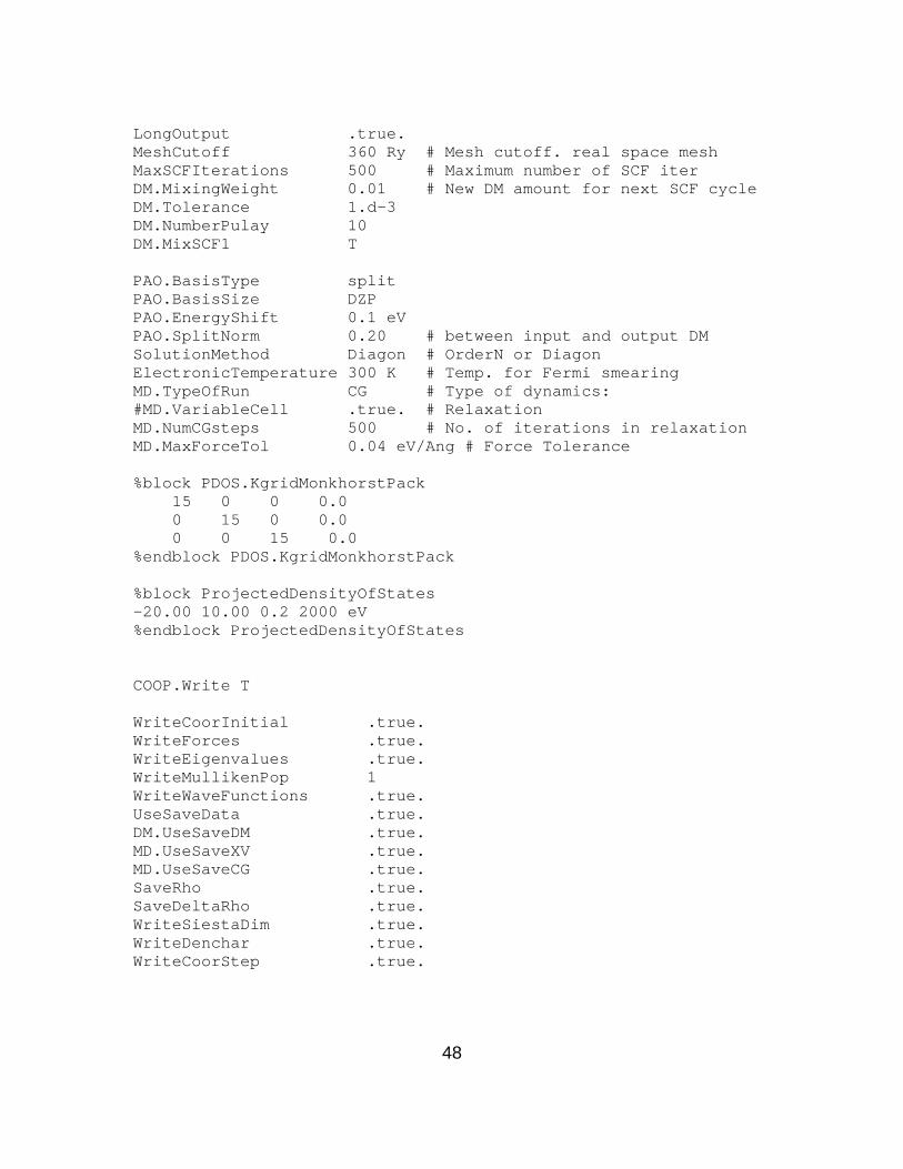
48

LongOutput .true. MeshCutoff 360 Ry # Mesh cutoff. real space mesh MaxSCFIterations 500 # Maximum number of SCF iter DM.MixingWeight 0.01 # New DM amount for next SCF cycle DM.Tolerance 1.d-3 DM.NumberPulay 10 DM.MixSCF1 T PAO.BasisType split PAO.BasisSize DZP PAO.EnergyShift 0.1 eV PAO.SplitNorm 0.20 # between input and output DM SolutionMethod Diagon # OrderN or Diagon ElectronicTemperature 300 K # Temp. for Fermi smearing MD.TypeOfRun CG # Type of dynamics: #MD.VariableCell .true. # Relaxation MD.NumCGsteps 500 # No. of iterations in relaxation MD.MaxForceTol 0.04 eV/Ang # Force Tolerance %block PDOS.KgridMonkhorstPack 15 0 0 0.0 0 15 0 0.0 0 0 15 0.0 %endblock PDOS.KgridMonkhorstPack %block ProjectedDensityOfStates -20.00 10.00 0.2 2000 eV %endblock ProjectedDensityOfStates COOP.Write T WriteCoorInitial .true. WriteForces .true. WriteEigenvalues .true. WriteMullikenPop 1 WriteWaveFunctions .true. UseSaveData .true. DM.UseSaveDM .true. MD.UseSaveXV .true. MD.UseSaveCG .true. SaveRho .true. SaveDeltaRho .true. WriteSiestaDim .true. WriteDenchar .true. WriteCoorStep .true.

49

APPENDIX B. SLURM CODE SNIPPET

#!/bin/bash #SBATCH --nodes=1 #SBATCH --ntasks-per-node=64 #SBATCH --mem-per-cpu=400M #SBATCH --time=72:00:00 #SBATCH --job-name=LiGr_02 #SBATCH --account=MyProjectName #####SBATCH --export=NONE source /etc/profile cd $SLURM_SUBMIT_DIR module load compile/intel/17.0 mpi/openmpi/2.0.1 mpirun -np 64 /work/smalnemr/siesta-3.1.t/Obj/siesta < Cluster.fdf | tee test_opt_1fluoroAlCp.out

50


51

INITIAL DISTRIBUTION LIST

1. Defense Technical Information Center Ft. Belvoir, Virginia 2. Dudley Knox Library Naval Postgraduate School Monterey, California

metalloid aluminum clusters with fluorine · metalloid aluminum clusters with fluorine 5. ... 16....

Documents