meta-dataset: a dataset of datasets for ...published as a conference paper at iclr 2020 meta-dataset...
TRANSCRIPT

Published as a conference paper at ICLR 2020
META-DATASET: A DATASET OF DATASETS FORLEARNING TO LEARN FROM FEW EXAMPLES
Eleni Triantafillou∗†, Tyler Zhu†, Vincent Dumoulin†, Pascal Lamblin†, Utku Evci†,Kelvin Xu‡†, Ross Goroshin†, Carles Gelada†, Kevin Swersky†,Pierre-Antoine Manzagol† & Hugo Larochelle†∗University of Toronto and Vector Institute, †Google AI, ‡University of California, BerkeleyCorrespondence to: [email protected]
ABSTRACT
Few-shot classification refers to learning a classifier for new classes given only afew examples. While a plethora of models have emerged to tackle it, we find theprocedure and datasets that are used to assess their progress lacking. To addressthis limitation, we propose META-DATASET: a new benchmark for training andevaluating models that is large-scale, consists of diverse datasets, and presentsmore realistic tasks. We experiment with popular baselines and meta-learnerson META-DATASET, along with a competitive method that we propose. Weanalyze performance as a function of various characteristics of test tasks andexamine the models’ ability to leverage diverse training sources for improving theirgeneralization. We also propose a new set of baselines for quantifying the benefit ofmeta-learning in META-DATASET. Our extensive experimentation has uncoveredimportant research challenges and we hope to inspire work in these directions.
1 INTRODUCTION
Few-shot learning refers to learning new concepts from few examples, an ability that humans naturallypossess, but machines still lack. Improving on this aspect would lead to more efficient algorithmsthat can flexibly expand their knowledge without requiring large labeled datasets. We focus onfew-shot classification: classifying unseen examples into one of N new ‘test’ classes, given only afew reference examples of each. Recent progress in this direction has been made by considering ameta-problem: though we are not interested in learning about any training class in particular, we canexploit the training classes for the purpose of learning to learn new classes from few examples, thusacquiring a learning procedure that can be directly applied to new few-shot learning problems too.
This intuition has inspired numerous models of increasing complexity (see Related Work for someexamples). However, we believe that the commonly-used setup for measuring success in this directionis lacking. Specifically, two datasets have emerged as de facto benchmarks for few-shot learning:Omniglot (Lake et al., 2015), and mini-ImageNet (Vinyals et al., 2016), and we believe that bothof them are approaching their limit in terms of allowing one to discriminate between the merits ofdifferent approaches. Omniglot is a dataset of 1623 handwritten characters from 50 different alphabetsand contains 20 examples per class (character). Most recent methods obtain very high accuracyon Omniglot, rendering the comparisons between them mostly uninformative. mini-ImageNet isformed out of 100 ImageNet (Russakovsky et al., 2015) classes (64/16/20 for train/validation/test)and contains 600 examples per class. Albeit harder than Omniglot, it has the same property thatmost recent methods trained on it present similar accuracy when controlling for model capacity. Weadvocate that a more challenging and realistic benchmark is required for further progress in this area.
More specifically, current benchmarks: 1) Consider homogeneous learning tasks. In contrast, real-lifelearning experiences are heterogeneous: they vary in terms of the number of classes and examplesper class, and are unbalanced. 2) Measure only within-dataset generalization. However, we areeventually after models that can generalize to entirely new distributions (e.g., datasets). 3) Ignore therelationships between classes when forming episodes. Specifically, the coarse-grained classificationof dogs and chairs may present different difficulties than the fine-grained classification of dog breeds,and current benchmarks do not establish a distinction between the two.
1
arX
iv:1
903.
0309
6v4
[cs
.LG
] 8
Apr
202
0
Published as a conference paper at ICLR 2020
META-DATASET aims to improve upon previous benchmarks in the above directions: it is significantlylarger-scale and is comprised of multiple datasets of diverse data distributions; its task creation isinformed by class structure for ImageNet and Omniglot; it introduces realistic class imbalance; and itvaries the number of classes in each task and the size of the training set, thus testing the robustness ofmodels across the spectrum from very-low-shot learning onwards.
The main contributions of this work are: 1) A more realistic, large-scale and diverse environment fortraining and testing few-shot learners. 2) Experimental evaluation of popular models, and a new set ofbaselines combining inference algorithms of meta-learners with non-episodic training. 3) Analyses ofwhether different models benefit from more data, heterogeneous training sources, pre-trained weights,and meta-training. 4) A novel meta-learner that performs strongly on META-DATASET.
2 FEW-SHOT CLASSIFICATION: TASK FORMULATION AND APPROACHES
Task Formulation The end-goal of few-shot classification is to produce a model which, given anew learning episode with N classes and a few labeled examples (kc per class, c ∈ 1, . . . , N ), isable to generalize to unseen examples for that episode. In other words, the model learns from atraining (support) set S = {(x1, y1), (x2, y2), . . . , (xK , yK)} (with K =
∑c kc) and is evaluated on
a held-out test (query) setQ = {(x∗1, y∗1), (x∗2, y∗2), . . . , (x∗T , y∗T )}. Each example (x, y) is formed ofan input vector x ∈ RD and a class label y ∈ {1, . . . , N}. Episodes with balanced training sets (i.e.,kc = k, ∀c) are usually described as ‘N -way, k-shot’ episodes. Evaluation episodes are constructedby sampling their N classes from a larger set Ctest of classes and sampling the desired number ofexamples per class.
A disjoint set Ctrain of classes is available to train the model; note that this notion of training isdistinct from the training that occurs within a few-shot learning episode. Few-shot learning does notprescribe a specific procedure for exploiting Ctrain, but a common approach matches the conditionsin which the model is trained and evaluated (Vinyals et al., 2016). In other words, training often (butnot always) proceeds in an episodic fashion. Some authors use training and testing to refer to whathappens within any given episode, and meta-training and meta-testing to refer to using Ctrain to turnthe model into a learner capable of fast adaptation and Ctest for evaluating its success to learn usingfew shots, respectively. This nomenclature highlights the meta-learning perspective alluded to earlier,but to avoid confusion we will adopt another common nomenclature and refer to the training and testsets of an episode as the support and query sets and to the process of learning from Ctrain simply astraining. We use the term ‘meta-learner’ to describe a model that is trained episodically, i.e., learns tolearn across multiple tasks that are sampled from the training set Ctrain.
Non-episodic Approaches to Few-shot Classification A natural non-episodic approach simplytrains a classifier over all of the training classes Ctrain at once, which can be parameterized by aneural network with a linear layer on top with one output unit per class. After training, this neuralnetwork is used as an embedding function g that maps images into a meaningful representation space.The hope of using this model for few-shot learning is that this representation space is useful even forexamples of classes that were not included in training. It would then remain to define an algorithmfor performing few-shot classification on top of these representations of the images of a task. Weconsider two choices for this algorithm, yielding the ‘k-NN’ and ‘Finetune’ variants of this baseline.
Given a test episode, the ‘k-NN’ baseline classifies each query example as the class that its ‘closest’support example belongs to. Closeness is measured by either Euclidean or cosine distance in thelearned embedding space; a choice that we treat as a hyperparameter. On the other hand, the ‘Finetune’baseline uses the support set of the given test episode to train a new ‘output layer’ on top of theembeddings g, and optionally finetune those embedding too (another hyperparameter), for the purposeof classifying between the N new classes of the associated task.
A variant of the ‘Finetune’ baseline has recently become popular: Baseline++ (Chen et al., 2019),originally inspired by Gidaris & Komodakis (2018); Qi et al. (2018). It uses a ‘cosine classifier’ asthe final layer (`2-normalizing embeddings and weights before taking the dot product), both duringthe non-episodic training phase, and for evaluation on test episodes. We incorporate this idea in ourcodebase by adding a hyperparameter that optionally enables using a cosine classifier for the ‘k-NN’(training only) and ‘Finetune’ (both phases) baselines.
2

Published as a conference paper at ICLR 2020
Meta-Learners for Few-shot Classification In the episodic setting, models are trained end-to-endfor the purpose of learning to build classifiers from a few examples. We choose to experimentwith Matching Networks (Vinyals et al., 2016), Relation Networks (Sung et al., 2018), PrototypicalNetworks (Snell et al., 2017) and Model Agnostic Meta-Learning (MAML, Finn et al., 2017) sincethey cover a diverse set of approaches to few-shot learning. We also introduce a novel meta-learnerwhich is inspired by the last two models.
In each training episode, episodic models compute for each query example x∗ ∈ Q, the distributionfor its label p(y∗|x∗,S) conditioned on the support set S and allow to train this differentiably-parameterized conditional distribution end-to-end via gradient descent. The different models aredistinguished by the manner in which this conditioning on the support set is realized. In all cases, theperformance on the query set drives the update of the meta-learner’s weights, which include (andsometimes consist only of) the embedding weights. We briefly describe each method below.
Prototypical Networks Prototypical Networks construct a prototype for each class and then classifyeach query example as the class whose prototype is ‘nearest’ to it under Euclidean distance. Moreconcretely, the probability that a query example x∗ belongs to class k is defined as:
p(y∗ = k|x∗,S) = exp(−||g(x∗)− ck||22)∑k′∈{1,...,N} exp(−||g(x∗)− ck′ ||22)
where ck is the ‘prototype’ for class k: the average of the embeddings of class k’s support examples.
Matching Networks Matching Networks (in their simplest form) label each query example as a(cosine) distance-weighted linear combination of the support labels:
p(y∗ = k|x∗,S) =|S|∑i=1
α(x∗,xi)1yi=k,
where 1A is the indicator function and α(x∗,xi) is the cosine similarity between g(x∗) and g(xi),softmax-normalized over all support examples xi, where 1 ≤ i ≤ |S|.
Relation Networks Relation Networks are comprised of an embedding function g as usual, anda ‘relation module’ parameterized by some additional neural network layers. They first embedeach support and query using g and create a prototype pc for each class c by averaging its supportembeddings. Each prototype pc is concatenated with each embedded query and fed through therelation module which outputs a number in [0, 1] representing the predicted probability that that querybelongs to class c. The query loss is then defined as the mean square error of that prediction comparedto the (binary) ground truth. Both g and the relation module are trained to minimize this loss.
MAML MAML uses a linear layer parametrized by W and b on top of the embedding functiong(·; θ) and classifies a query example as
p(y∗|x∗,S) = softmax(b′ +W′g(x∗; θ′)),
where the output layer parameters W′ and b′ and the embedding function parameters θ′ are obtainedby performing a small number of within-episode training steps on the support set S, starting frominitial parameter values (b,W, θ). The model is trained by backpropagating the query set lossthrough the within-episode gradient descent procedure and into (b,W, θ). This normally requirescomputing second-order gradients, which can be expensive to obtain (both in terms of time andmemory). For this reason, an approximation is often used whereby gradients of the within-episodedescent steps are ignored. This variant is referred to as first-order MAML (fo-MAML) and was usedin our experiments. We did attempt to use the full-order version, but found it to be impracticallyexpensive (e.g., it caused frequent out-of-memory problems).
Moreover, since in our setting the number of ways varies between episodes, b,W are set to zero andare not trained (i.e., b′,W′ are the result of within-episode gradient descent initialized at 0), leavingonly θ to be trained. In other words, MAML focuses on learning the within-episode initialization θ ofthe embedding network so that it can be rapidly adapted for a new task.
3

Published as a conference paper at ICLR 2020
Introducing Proto-MAML We introduce a novel meta-learner that combines the complementarystrengths of Prototypical Networks and MAML: the former’s simple inductive bias that is evidentlyeffective for very-few-shot learning, and the latter’s flexible adaptation mechanism.
As explained by Snell et al. (2017), Prototypical Networks can be re-interpreted as a linear classifierapplied to a learned representation g(x). The use of a squared Euclidean distance means that outputlogits are expressed as
−||g(x∗)− ck||2 = −g(x∗)T g(x∗) + 2cTk g(x∗)− cTk ck = 2cTk g(x
∗)− ||ck||2 + constant
where constant is a class-independent scalar which can be ignored, as it leaves output probabilitiesunchanged. The k-th unit of the equivalent linear layer therefore has weights Wk,· = 2ck and biasesbk = −||ck||2, which are both differentiable with respect to θ as they are a function of g(·; θ).We refer to (fo-)Proto-MAML as the (fo-)MAML model where the task-specific linear layer of eachepisode is initialized from the Prototypical Network-equivalent weights and bias defined above andsubsequently optimized as usual on the given support set. When computing the update for θ, weallow gradients to flow through the Prototypical Network-equivalent linear layer initialization. Weshow that this simple modification significantly helps the optimization of this model and outperformsvanilla fo-MAML by a large margin on META-DATASET.
3 META-DATASET: A NEW FEW-SHOT CLASSIFICATION BENCHMARK
META-DATASET aims to offer an environment for measuring progress in realistic few-shot classifica-tion tasks. Our approach is twofold: 1) changing the data and 2) changing the formulation of the task(i.e., how episodes are generated). The following sections describe these modifications in detail. Thecode is open source and publicly available1.
3.1 META-DATASET’S DATA
META-DATASET’s data is much larger in size than any previous benchmark, and is comprised ofmultiple existing datasets. This invites research into how diverse sources of data can be exploitedby a meta-learner, and allows us to evaluate a more challenging generalization problem, to newdatasets altogether. Specifically, META-DATASET leverages data from the following 10 datasets:ILSVRC-2012 (ImageNet, Russakovsky et al., 2015), Omniglot (Lake et al., 2015), Aircraft (Majiet al., 2013), CUB-200-2011 (Birds, Wah et al., 2011), Describable Textures (Cimpoi et al., 2014),Quick Draw (Jongejan et al., 2016), Fungi (Schroeder & Cui, 2018), VGG Flower (Nilsback &Zisserman, 2008), Traffic Signs (Houben et al., 2013) and MSCOCO (Lin et al., 2014). Thesedatasets were chosen because they are free and easy to obtain, span a variety of visual concepts(natural and human-made) and vary in how fine-grained the class definition is. More informationabout each of these datasets is provided in the Appendix.
To ensure that episodes correspond to realistic classification problems, each episode generated inMETA-DATASET uses classes from a single dataset. Moreover, two of these datasets, Traffic Signsand MSCOCO, are fully reserved for evaluation, meaning that no classes from them participate inthe training set. The remaining ones contribute some classes to each of the training, validation andtest splits of classes, roughly with 70% / 15% / 15% proportions. Two of these datasets, ImageNetand Omniglot, possess a class hierarchy that we exploit in META-DATASET. For each dataset, thecomposition of splits is available online2.
ImageNet ImageNet is comprised of 82,115 ‘synsets’, i.e., concepts of the WordNet ontology, andit provides ‘is-a’ relationships for its synsets, thus defining a DAG over them. META-DATASET usesthe 1K synsets that were chosen for the ILSVRC 2012 classification challenge and defines a new classsplit for it and a novel procedure for sampling classes from it for episode creation, both informed byits class hierarchy.
Specifically, we construct a sub-graph of the overall DAG whose leaves are the 1K classes of ILSVRC-2012. We then ‘cut’ this sub-graph into three pieces, for the training, validation, and test splits,
1github.com/google-research/meta-dataset2github.com/google-research/meta-dataset/tree/master/meta_dataset/dataset_conversion/splits
4

Published as a conference paper at ICLR 2020
such that there is no overlap between the leaves of any of these pieces. For this, we selected thesynsets ‘carnivore’ and ‘device’ as the roots of the validation and test sub-graphs, respectively. Theleaves that are reachable from ‘carnivore’ and ‘device’ form the sets of the validation and test classes,respectively. All of the remaining leaves constitute the training classes. This method of splittingensures that the training classes are semantically different from the test classes. We end up with 712training, 158 validation and 130 test classes, roughly adhering to the standard 70 / 15 / 15 (%) splits.
Omniglot This dataset is one of the established benchmarks for few-shot classification as men-tioned earlier. However, contrary to the common setup that flattens and ignores its two-level hierarchyof alphabets and characters, we allow it to influence the episode class selection in META-DATASET,yielding finer-grained tasks. We also use the original splits proposed in Lake et al. (2015): (all char-acters of) the ‘background’ and ‘evaluation’ alphabets are used for training and testing, respectively.However, we reserve the 5 smallest alphabets from the ‘background’ set for validation.
3.2 EPISODE SAMPLING
In this section we outline META-DATASET’s algorithm for sampling episodes, featuring hierarchically-aware procedures for sampling classes of ImageNet and Omniglot, and an algorithm that yieldsrealistically imbalanced episodes of variable shots and ways. The steps for sampling an episode fora given split are: Step 0) uniformly sample a dataset D, Step 1) sample a set of classes C from theclasses of D assigned to the requested split, and Step 2) sample support and query examples from C.
Step 1: Sampling the episode’s class set This procedure differs depending on which dataset ischosen. For datasets without a known class organization, we sample the ‘way’ uniformly from therange [5,MAX-CLASSES], where MAX-CLASSES is either 50 or as many as there are available.Then we sample ‘way’ many classes uniformly at random from the requested class split of the givendataset. ImageNet and Omniglot use class-structure-aware procedures outlined below.
ImageNet class sampling We adopt a hierarchy-aware sampling procedure: First, we sample aninternal (non-leaf) node uniformly from the DAG of the given split. The chosen set of classes is thenthe set of leaves spanned by that node (or a random subset of it, if more than 50). We prevent nodesthat are too close to the root to be selected as the internal node, as explained in more detail in theAppendix. This procedure enables the creation of tasks of varying degrees of fine-grainedness: thelarger the height of the internal node, the more coarse-grained the resulting episode.
Omniglot class sampling We sample classes from Omniglot by first sampling an alphabet uni-formly at random from the chosen split of alphabets (train, validation or test). Then, the ‘way’ of theepisode is sampled uniformly at random using the same restrictions as for the rest of the datasets, buttaking care not to sample a larger number than the number of characters that belong to the chosenalphabet. Finally, the prescribed number of characters of that alphabet are randomly sampled. Thisensures that each episode presents a within-alphabet fine-grained classification.
Step 2: Sampling the episode’s examples Having already selected a set of classes, the choiceof the examples from them that will populate an episode can be broken down into three steps. Weprovide a high-level description here and elaborate in the Appendix with the accompanying formulas.
Step 2a: Compute the query set size The query set is class-balanced, reflecting the fact that wecare equally to perform well on all classes of an episode. The number of query images per class isset to a number such that all chosen classes have enough images to contribute that number and stillremain with roughly half on their images to possibly add to the support set (in a later step). Thisnumber is capped to 10 images per class.
Step 2b: Compute the support set size We allow each chosen class to contribute to the support setat most 100 of its remaining examples (i.e., excluding the ones added to the query set). We multiplythis remaining number by a scalar sampled uniformly from the interval (0, 1] to enable the potentialgeneration of ‘few-shot’ episodes even when multiple images are available, as we are also interestedin studying that end of the spectrum. We do enforce, however, that each chosen class has a budget forat least one image in the support set, and we cap the total support set size to 500 examples.
5

Published as a conference paper at ICLR 2020
Step 2c: Compute the shot of each class We now discuss how to distribute the total support setsize chosen above across the participating classes. The un-normalized proportion of the support setthat will be occupied by a given chosen class is a noisy version of the total number of images ofthat class in the dataset. This design choice is made in the hopes of obtaining realistic class ratios,under the hypothesis that the dataset class statistics are a reasonable approximation of the real-worldstatistics of appearances of the corresponding classes. We ensure that each class has at least oneimage in the support set and distribute the rest according to the above rule.
After these steps, we complete the episode creation process by choosing the prescribed number ofexamples of each chosen class uniformly at random to populate the support and query sets.
4 RELATED WORK
In this work we evaluate four meta-learners on META-DATASET that we believe capture a gooddiversity of well-established models. Evaluating other few-shot classifiers on META-DATASET isbeyond the scope of this paper, but we discuss some additional related models below.
Similarly to MAML, some train a meta-learner for quick adaptation to new tasks (Ravi & Larochelle,2017; Munkhdalai & Yu, 2017; Rusu et al., 2019; Yoon et al., 2018). Others relate to PrototypicalNetworks by learning a representation on which differentiable training can be performed on some formof classifier (Bertinetto et al., 2019; Gidaris & Komodakis, 2018; Oreshkin et al., 2018). Others relateto Matching Networks in that they perform comparisons between pairs of support and query examples,using either a graph neural network (Satorras & Estrach, 2018) or an attention mechanism (Mishraet al., 2018). Finally, some make use of memory-augmented recurrent networks (Santoro et al.,2016), some learn to perform data augmentation (Hariharan & Girshick, 2017; Wang et al., 2018) ina low-shot learning setting, and some learn to predict the parameters of a large-shot classifier fromthe parameters learned in a few-shot setting (Wang & Hebert, 2016; Wang et al., 2017). Of relevanceto Proto-MAML is MAML++ (Antoniou et al., 2019), which consists of a collection of adjustmentsto MAML, such as multiple meta-trained inner loop learning rates and derivative-order annealing.Proto-MAML instead modifies the output weight initialization scheme and could be combined withthose adjustments.
Finally, META-DATASET relates to other recent image classification benchmarks. The CVPR2017 Visual Domain Decathlon Challenge trains a model on 10 different datasets, many of whichare included in our benchmark, and measures its ability to generalize to held-out examples forthose same datasets but does not measure generalization to new classes (or datasets). Hariharan& Girshick (2017) propose a benchmark where a model is given abundant data from certain baseImageNet classes and is tested on few-shot learning novel ImageNet classes in a way that doesn’tcompromise its knowledge of the base classes. Wang et al. (2018) build upon that benchmarkand propose a new evaluation protocol for it. Chen et al. (2019) investigate fine-grained few-shotclassification using the CUB dataset (Wah et al., 2011, also featured in our benchmark) and cross-domain transfer between mini-ImageNet and CUB. Larger-scale few-shot classification benchmarkswere also proposed using CIFAR-100 (Krizhevsky et al., 2009; Bertinetto et al., 2019; Oreshkin et al.,2018), tiered-ImageNet (Ren et al., 2018), and ImageNet-21k (Dhillon et al., 2019). Compared tothese, META-DATASET contains the largest set of diverse datasets in the context of few-shot learningand is additionally accompanied by an algorithm for creating learning scenarios from that data thatwe advocate are more realistic than the previous ones.
5 EXPERIMENTS
Training procedure META-DATASET does not prescribe a procedure for learning from the trainingdata. In these experiments, keeping with the spirit of matching training and testing conditions, wetrained the meta-learners via training episodes sampled using the same algorithm as we used forMETA-DATASET’s evaluation episodes, described above. The choice of the dataset from which tosample the next episode was random uniform. The non-episodic baselines are trained to solve thelarge classification problem that results from ‘concatenating’ the training classes of all datasets.
Validation Another design choice was to perform validation on (the validation split of) ImageNetonly, ignoring the validation sets of the other datasets. The rationale behind this choice is that the
6
Published as a conference paper at ICLR 2020
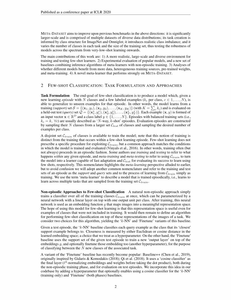
Table 1: Few-shot classification results on META-DATASET using models trained on ILSVRC-2012only (top) and trained on all datasets (bottom).
Test Source k-NN Finetune MatchingNet ProtoNet fo-MAML RelationNet fo-Proto-MAMLILSVRC 41.03 45.78 45.00 50.50 45.51 34.69 49.53Omniglot 37.07 60.85 52.27 59.98 55.55 45.35 63.37Aircraft 46.81 68.69 48.97 53.10 56.24 40.73 55.95Birds 50.13 57.31 62.21 68.79 63.61 49.51 68.66
Textures 66.36 69.05 64.15 66.56 68.04 52.97 66.49Quick Draw 32.06 42.60 42.87 48.96 43.96 43.30 51.52
Fungi 36.16 38.20 33.97 39.71 32.10 30.55 39.96VGG Flower 83.10 85.51 80.13 85.27 81.74 68.76 87.15Traffic Signs 44.59 66.79 47.80 47.12 50.93 33.67 48.83MSCOCO 30.38 34.86 34.99 41.00 35.30 29.15 43.74Avg. rank 5.7 2.9 4.65 2.65 3.7 6.55 1.85
Test Source k-NN Finetune MatchingNet ProtoNet fo-MAML RelationNet fo-Proto-MAMLILSVRC 38.55 43.08 36.08 44.50 37.83 30.89 46.52Omniglot 74.60 71.11 78.25 79.56 83.92 86.57 82.69Aircraft 64.98 72.03 69.17 71.14 76.41 69.71 75.23Birds 66.35 59.82 56.40 67.01 62.43 54.14 69.88
Textures 63.58 69.14 61.80 65.18 64.16 56.56 68.25Quick Draw 44.88 47.05 60.81 64.88 59.73 61.75 66.84
Fungi 37.12 38.16 33.70 40.26 33.54 32.56 41.99VGG Flower 83.47 85.28 81.90 86.85 79.94 76.08 88.72Traffic Signs 40.11 66.74 55.57 46.48 42.91 37.48 52.42MSCOCO 29.55 35.17 28.79 39.87 29.37 27.41 41.74Avg. rank 5.05 3.6 4.95 2.85 4.25 5.8 1.5
performance on ImageNet has been known to be a good proxy for the performance on differentdatasets. We used this validation performance to select our hyperparameters, including backbonearchitectures, image resolutions and model-specific ones. We describe these further in the Appendix.
Pre-training We gave each meta-learner the opportunity to initialize its embedding function fromthe embedding weights to which the k-NN Baseline model trained on ImageNet converged to. Wetreated the choice of starting from scratch or starting from this initialization as a hyperparameter.For a fair comparison with the baselines, we allowed the non-episodic models to start from thisinitialization too. This is especially important for the baselines in the case of training on all datasetssince it offers the opportunity to start from ImageNet-pretrained weights.
Main results Table 1 displays the accuracy of each model on the test set of each dataset, after theywere trained on ImageNet-only or all datasets. Traffic Signs and MSCOCO are not used for trainingin either case, as they are reserved for evaluation. We propose to use the average (over the datasets)rank of each method as our metric for comparison, where smaller is better. A method receives rank 1if it has the highest accuracy, rank 2 if it has the second highest, and so on. If two models share thebest accuracy, they both get rank 1.5, and so on. We find that fo-Proto-MAML is the top-performeraccording to this metric, Prototypical Networks also perform strongly, and the Finetune Baselinenotably presents a worthy opponent3. We include more detailed versions of these tables displayingconfidence intervals and per-dataset ranks in the Appendix.
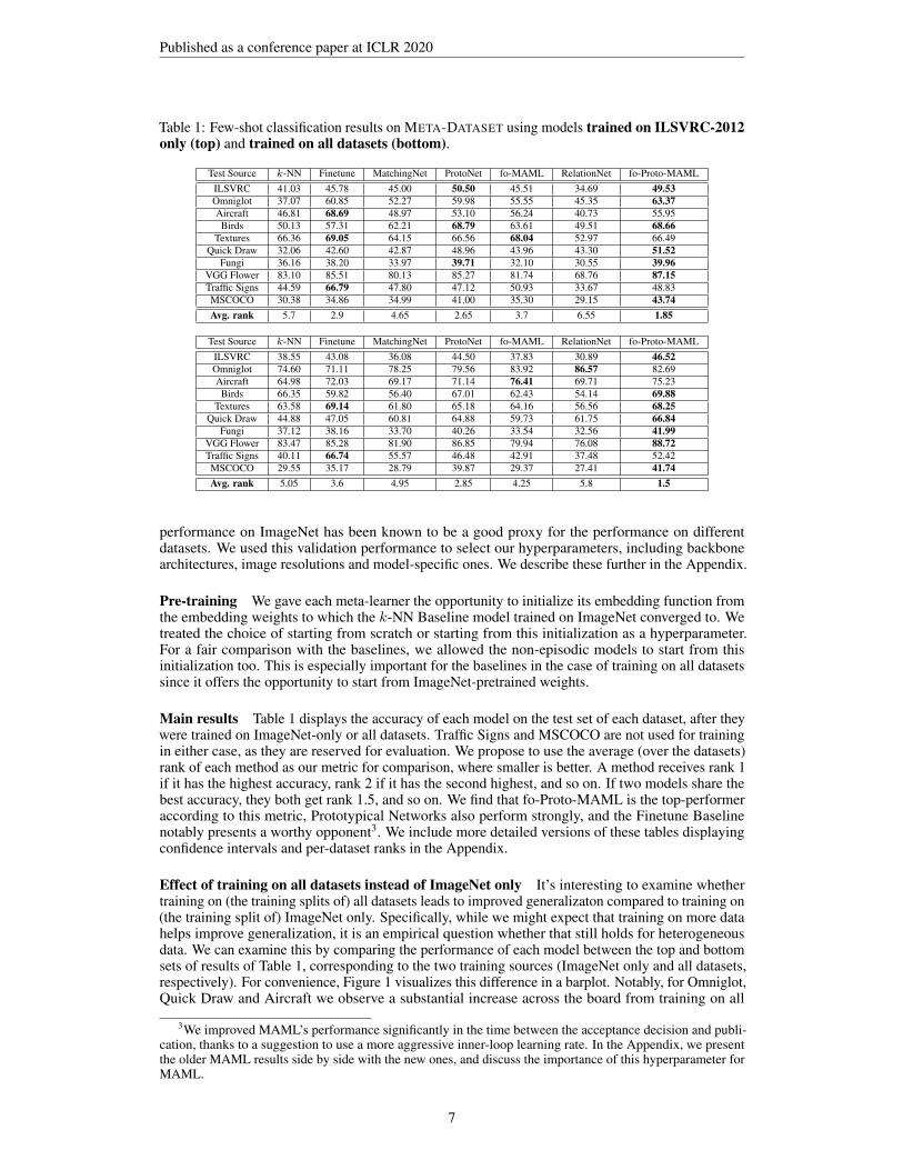
Effect of training on all datasets instead of ImageNet only It’s interesting to examine whethertraining on (the training splits of) all datasets leads to improved generalizaton compared to training on(the training split of) ImageNet only. Specifically, while we might expect that training on more datahelps improve generalization, it is an empirical question whether that still holds for heterogeneousdata. We can examine this by comparing the performance of each model between the top and bottomsets of results of Table 1, corresponding to the two training sources (ImageNet only and all datasets,respectively). For convenience, Figure 1 visualizes this difference in a barplot. Notably, for Omniglot,Quick Draw and Aircraft we observe a substantial increase across the board from training on all
3We improved MAML’s performance significantly in the time between the acceptance decision and publi-cation, thanks to a suggestion to use a more aggressive inner-loop learning rate. In the Appendix, we presentthe older MAML results side by side with the new ones, and discuss the importance of this hyperparameter forMAML.
7
Published as a conference paper at ICLR 2020
2010
01020304050 ILSVRC Omniglot Aircraft CU Birds Textures
Modelk-NN baseline
Finetune baseline
MatchingNet
ProtoNet
fo-MAML
RelationNet
fo-Proto-MAML
2010
01020304050 Quick Draw Fungi VGG Flower Traffic Sign MSCOCO
Figure 1: The performance difference on test datasets, when training on all datasets instead ofILSVRC only. A positive value indicates an improvement from all-dataset training.
sources. This is reasonable for datasets whose images are significantly different from ImageNet’s:we indeed expect to gain a large benefit from training on some images from (the training classes of)these datasets. Interestingly though, on the remainder of the test sources, we don’t observe a gainfrom all-dataset training. This result invites research into methods for exploiting heterogeneous datafor generalization to unseen classes of diverse sources. Our experiments show that learning ‘naively’across the training datasets (e.g., by picking the next dataset to use uniformly at random) does notautomatically lead to that desired benefit in most cases.
10 20 30 40 50Way
0.0
0.2
0.4
0.6
0.8
1.0
Acc
ura
cy
k-NN baseline
Finetune baseline
MatchingNet
ProtoNet
fo-MAML
RelationNet
fo-Proto-MAML
(a) Ways analysis
0 20 40 60 80 100Shot
0.0
0.2
0.4
0.6
0.8
Cla
ss P
reci
sion
k-NN baseline
Finetune baseline
MatchingNet
ProtoNet
fo-MAML
RelationNet
fo-Proto-MAML
(b) Shots analysis
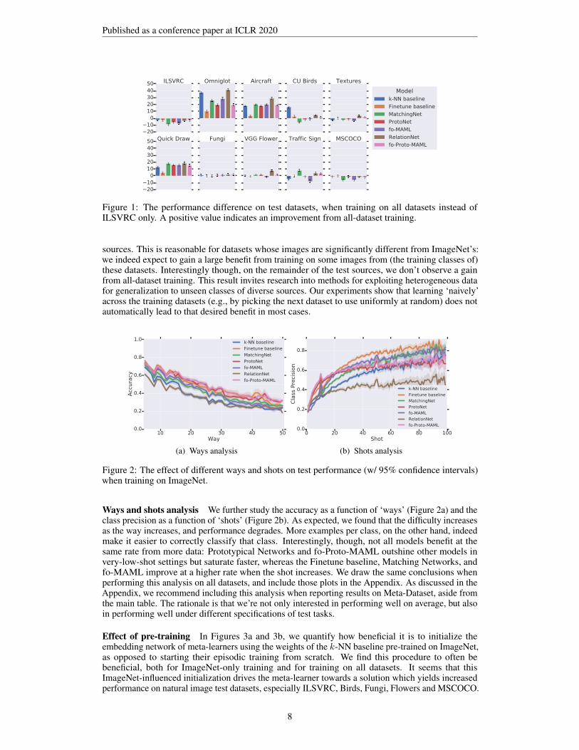
Figure 2: The effect of different ways and shots on test performance (w/ 95% confidence intervals)when training on ImageNet.
Ways and shots analysis We further study the accuracy as a function of ‘ways’ (Figure 2a) and theclass precision as a function of ‘shots’ (Figure 2b). As expected, we found that the difficulty increasesas the way increases, and performance degrades. More examples per class, on the other hand, indeedmake it easier to correctly classify that class. Interestingly, though, not all models benefit at thesame rate from more data: Prototypical Networks and fo-Proto-MAML outshine other models invery-low-shot settings but saturate faster, whereas the Finetune baseline, Matching Networks, andfo-MAML improve at a higher rate when the shot increases. We draw the same conclusions whenperforming this analysis on all datasets, and include those plots in the Appendix. As discussed in theAppendix, we recommend including this analysis when reporting results on Meta-Dataset, aside fromthe main table. The rationale is that we’re not only interested in performing well on average, but alsoin performing well under different specifications of test tasks.
Effect of pre-training In Figures 3a and 3b, we quantify how beneficial it is to initialize theembedding network of meta-learners using the weights of the k-NN baseline pre-trained on ImageNet,as opposed to starting their episodic training from scratch. We find this procedure to often bebeneficial, both for ImageNet-only training and for training on all datasets. It seems that thisImageNet-influenced initialization drives the meta-learner towards a solution which yields increasedperformance on natural image test datasets, especially ILSVRC, Birds, Fungi, Flowers and MSCOCO.
8

Published as a conference paper at ICLR 2020
0102030405060708090 ILSVRC Omniglot Aircraft CU Birds Textures
ModelMatchingNet
ProtoNet
fo-MAML
RelationNet
fo-Proto-MAML
0102030405060708090 Quick Draw Fungi VGG Flower Traffic Sign MSCOCO
InitializationPre-trained
From scratch
(a) Effect of pre-training (ImageNet)
0
20
40
60
80
100 ILSVRC Omniglot Aircraft CU Birds Textures
0
20
40
60
80
100 Quick Draw Fungi VGG Flower Traffic Sign MSCOCO
(b) Effect of pre-training (All datasets)
0102030405060708090 ILSVRC Omniglot Aircraft CU Birds Textures
ModelMatchingNet
ProtoNet
fo-Proto-MAML
0102030405060708090 Quick Draw Fungi VGG Flower Traffic Sign MSCOCO
Meta-training
Inference-only
(c) Effect of meta-learning (ImageNet)
0102030405060708090 ILSVRC Omniglot Aircraft CU Birds Textures
0102030405060708090 Quick Draw Fungi VGG Flower Traffic Sign MSCOCO
(d) Effect of meta-learning (All datasets)
Figure 3: The effects of pre-training and meta-training (w/ 95% confidence intervals). (ImageNet) or(All datasets) is the training source.
Perhaps unsusprisingly, though, it underperforms on significantly different datasets such as Omniglotand Quick Draw. These findings show that, aside from the choice of the training data source(s) (e.g.,ImageNet only or all datasets, as discussed above), the choice of the initialization scheme can alsoinfluence to an important degree the final solution and consequently the aptness of applying theresulting meta-learner to different data sources at test time. Finally, an interesting observation isthat MAML seems to benefit the most from the pre-trained initialization, which may speak to thedifficulty of optimization associated with that model.
Effect of meta-training We propose to disentangle the inference algorithm of each meta-learnerfrom the fact that it is meta-learned, to assess the benefit of meta-learning on META-DATASET.To this end, we propose a new set of baselines: ‘Prototypical Networks Inference’, ‘MatchingNetworks Inference’, and ‘fo-Proto-MAML Inference’, that are trained non-episodically but evaluatedepisodically (for validation and testing) using the inference algorithm of the respective meta-learner.This is possible for these meta-learners as they don’t have any additional parameters aside from theembedding function that explicitly need to be learned episodically (as opposed to the relation moduleof Relation Networks, for example). We compare each Inference-only method to its correspondingmeta-learner in Figures 3c and 3d. We find that these baselines are strong: when training on ImageNetonly, we can usually observe a small benefit from meta-learning the embedding weights but thisbenefit often disappears when training on all datasets, in which case meta-learning sometimes actuallyhurts. We find this result very interesting and we believe it emphasizes the need for research on howto meta-learn across multiple diverse sources, an important challenge that META-DATASET putsforth.
Fine-grainedness analysis We use ILVRC-2012 to investigate the hypothesis that finer-grainedtasks are harder than coarse-grained ones. Our findings suggest that while the test sub-graph is notrich enough to exhibit any trend, the performance on the train sub-graph does seem to agree with thishypothesis. We include the experimental setup and results for this analysis in the Appendix.
6 CONCLUSION
We have introduced a new large-scale, diverse, and realistic environment for few-shot classification.We believe that our exploration of various models on META-DATASET has uncovered interesting
9

Published as a conference paper at ICLR 2020
directions for future work pertaining to meta-learning across heterogeneous data: it remains unclearwhat is the best strategy for creating training episodes, the most appropriate validation creation andthe most appropriate initialization. Current models don’t always improve when trained on multiplesources and meta-learning is not always beneficial across datasets. Current models are also not robustto the amount of data in test episodes, each excelling in a different part of the spectrum. We believethat addressing these shortcomings consitutes an important research goal moving forward.
AUTHOR CONTRIBUTIONS
Eleni, Hugo, and Kevin came up with the benchmark idea and requirements. Eleni developed the coreof the project, and worked on the experiment design and management with Tyler and Kevin, as well asexperiment analysis. Carles, Ross, Kelvin, Pascal, Vincent, and Tyler helped extend the benchmark byadding datasets. Eleni, Vincent, and Utku contributed the Prototypical Networks, Matching Networks,and Relation Networks implementations, respectively. Tyler implemented baselines, MAML (withKevin) and Proto-MAML models, and updated the backbones to support them. Writing was mostlyled by Eleni, with contributions by Hugo, Vincent, and Kevin and help from Tyler and Pascal forvisualizations. Pascal and Pierre-Antoine worked on code organization, efficiency, and open-sourcing,Pascal and Vincent optimized the efficiency of the data input pipeline. Pierre-Antoine supervised thecode development process and reviewed most of the changes, Hugo and Kevin supervised the overalldirection of the research.
ACKNOWLEDGMENTS
We would like to thank Chelsea Finn for fruitful discussions and advice on tuning fo-MAML andensuring the correctness of implementation, as well as Zack Nado and Dan Moldovan for the initialdataset code that was adapted, and Cristina Vasconcelos for spotting an issue in the ranking ofmodels. Finally, we’d like to thank John Bronskill for suggesting that we experiment with a largerinner-loop learning rate for MAML which indeed significantly improved our fo-MAML results onMETA-DATASET.
10

Published as a conference paper at ICLR 2020
REFERENCES
Antreas Antoniou, Harrison Edwards, and Amos Storkey. How to train your MAML. In Proceedingsof the International Conference on Learning Representations, 2019.
Luca Bertinetto, Joao F. Henriques, Philip Torr, and Andrea Vedaldi. Meta-learning with differentiableclosed-form solvers. In Proceedings of the International Conference on Learning Representations,2019.
Wei-Yu Chen, Yen-Cheng Liu, Zsolt Kira, Yu-Chiang Frank Wang, and Jia-Bin Huang. A closerlook at few-shot classification. In Proceedings of the International Conference on LearningRepresentations, 2019.
M. Cimpoi, S. Maji, I. Kokkinos, S. Mohamed, and A. Vedaldi. Describing textures in the wild. InIEEE Conference on Computer Vision and Pattern Recognition, 2014.
Guneet S. Dhillon, Pratik Chaudhari, Avinash Ravichandran, and Stefano Soatto. A baseline forfew-shot image classification. arXiv, abs/1909.02729, 2019.
Chelsea Finn, Pieter Abbeel, and Sergey Levine. Model-agnostic meta-learning for fast adaptation ofdeep networks. In Proceedings of the International Conference of Machine Learning, 2017.
Spyros Gidaris and Nikos Komodakis. Dynamic few-shot visual learning without forgetting. In IEEEConference on Computer Vision and Pattern Recognition, 2018.
Bharath Hariharan and Ross Girshick. Low-shot visual recognition by shrinking and hallucinatingfeatures. In Proceedings of the IEEE International Conference on Computer Vision, pp. 3018–3027,2017.
Sebastian Houben, Johannes Stallkamp, Jan Salmen, Marc Schlipsing, and Christian Igel. Detection oftraffic signs in real-world images: The German Traffic Sign Detection Benchmark. In InternationalJoint Conference on Neural Networks, 2013.
Jonas Jongejan, Henry Rowley, Takashi Kawashima, Jongmin Kim, and Nick Fox-Gieg. The Quick,Draw! – A.I. experiment. quickdraw.withgoogle.com, 2016.
Alex Krizhevsky et al. Learning multiple layers of features from tiny images. Technical report,University of Toronto, 2009.
Brenden M Lake, Ruslan Salakhutdinov, and Joshua B Tenenbaum. Human-level concept learningthrough probabilistic program induction. Science, 350(6266):1332–1338, 2015.
Tsung-Yi Lin, Michael Maire, Serge Belongie, James Hays, Pietro Perona, Deva Ramanan, PiotrDollár, and C Lawrence Zitnick. Microsoft COCO: Common objects in context. In EuropeanConference on Computer Vision, pp. 740–755, 2014.
Subhransu Maji, Esa Rahtu, Juho Kannala, Matthew Blaschko, and Andrea Vedaldi. Fine-grainedvisual classification of aircraft. arXiv, abs/1306.5151, 2013.
Nikhil Mishra, Mostafa Rohaninejad, Xi Chen, and Pieter Abbeel. A simple neural attentive meta-learner. In Proceedings of the International Conference on Learning Representations, 2018.
Tsendsuren Munkhdalai and Hong Yu. Meta networks. In Proceedings of the International Conferenceon Machine Learning, pp. 2554–2563, 2017.
M-E. Nilsback and A. Zisserman. Automated flower classification over a large number of classes. InProceedings of the Indian Conference on Computer Vision, Graphics and Image Processing, 2008.
Boris N. Oreshkin, Pau Rodriguez, and Alexandre Lacoste. TADAM: Task dependent adaptivemetric for improved few-shot learning. In Advances in Neural Information Processing Systems, pp.719–729, 2018.
Hang Qi, Matthew Brown, and David G Lowe. Low-shot learning with imprinted weights. InProceedings of the IEEE Conference on Computer Vision and Pattern Recognition, pp. 5822–5830,2018.
11

Published as a conference paper at ICLR 2020
Sachin Ravi and Hugo Larochelle. Optimization as a model for few-shot learning. In Proceedings ofthe International Conference on Learning Representations, 2017.
Mengye Ren, Eleni Triantafillou, Sachin Ravi, Jake Snell, Kevin Swersky, Joshua B Tenenbaum,Hugo Larochelle, and Richard S Zemel. Meta-learning for semi-supervised few-shot classification.In Proceedings of the International Conference on Learning Representations, 2018.
Olga Russakovsky, Jia Deng, Hao Su, Jonathan Krause, Sanjeev Satheesh, Sean Ma, Zhiheng Huang,Andrej Karpathy, Aditya Khosla, Michael Bernstein, Alexander C Berg, and Li Fei-Fei. Imagenetlarge scale visual recognition challenge. International Journal of Computer Vision, 115(3):211–252,2015.
Andrei A. Rusu, Dushyant Rao, Jakub Sygnowski, Oriol Vinyals, Razvan Pascanu, Simon Osindero,and Raia Hadsell. Meta-learning with latent embedding optimization. In Proceedings of theInternational Conference on Learning Representations, 2019.
Tim Salimans and Durk P Kingma. Weight normalization: A simple reparameterization to acceleratetraining of deep neural networks. In Advances in Neural Information Processing Systems, pp.901–909, 2016.
Adam Santoro, Sergey Bartunov, Matthew Botvinick, Daan Wierstra, and Timothy Lillicrap. Meta-learning with memory-augmented neural networks. In Proceedings of the International Conferenceon Machine Learning, pp. 1842–1850, 2016.
Victor Garcia Satorras and Joan Bruna Estrach. Few-shot learning with graph neural networks. InProceedings of the International Conference on Learning Representations, 2018.
Brigit Schroeder and Yin Cui. FGVCx fungi classification challenge 2018. github.com/visipedia/fgvcx_fungi_comp, 2018.
Jake Snell, Kevin Swersky, and Richard Zemel. Prototypical networks for few-shot learning. InAdvances in Neural Information Processing Systems, pp. 4077–4087, 2017.
Flood Sung, Yongxin Yang, Li Zhang, Tao Xiang, Philip HS Torr, and Timothy M Hospedales.Learning to compare: Relation network for few-shot learning. In Proceedings of the IEEEConference on Computer Vision and Pattern Recognition, pp. 1199–1208, 2018.
Oriol Vinyals, Charles Blundell, Tim Lillicrap, and Daan Wierstra. Matching networks for one shotlearning. In Advances in Neural Information Processing Systems, pp. 3630–3638, 2016.
C. Wah, S. Branson, P. Welinder, P. Perona, and S. Belongie. The Caltech-UCSD Birds-200-2011Dataset. Technical Report CNS-TR-2011-001, California Institute of Technology, 2011.
Yu-Xiong Wang and Martial Hebert. Learning to learn: Model regression networks for easy smallsample learning. In European Conference on Computer Vision, pp. 616–634. Springer, 2016.
Yu-Xiong Wang, Deva Ramanan, and Martial Hebert. Learning to model the tail. In Advances inNeural Information Processing Systems, pp. 7029–7039, 2017.
Yu-Xiong Wang, Ross Girshick, Martial Hebert, and Bharath Hariharan. Low-shot learning fromimaginary data. In Proceedings of the IEEE Conference on Computer Vision and Pattern Recogni-tion, pp. 7278–7286, 2018.
Jaesik Yoon, Taesup Kim, Ousmane Dia, Sungwoong Kim, Yoshua Bengio, and Sungjin Ahn.Bayesian model-agnostic meta-learning. In Advances in Neural Information Processing Systems,2018.
12

Published as a conference paper at ICLR 2020
APPENDIX
.1 RECOMMENDATION FOR REPORTING RESULTS ON META-DATASET
We recommend that future work on META-DATASET reports two sets of results:
1. The main tables storing the average (over 600 test episodes) accuracy of each method oneach dataset, after it has been trained on ImageNet only and on All datasets, where theevaluation metric is the average rank. This corresponds to Table 1 in our case (or the morecomplete version in Table 2 in the Appendix).
2. The plots that measure robustness in variations of shots and ways. In our case these areFigures 2b and 2a in the main text for ImageNet-only training, and Figures 5b and 5a in theAppendix for the case of training on all datasets.
We propose to use both of these aspects to evaluate performance on META-DATASET: it is not onlydesirable to perform well on average, but also to perform well under different specifications of testtasks, as it is not realistic in general to assume that we will know in advance what setup (numberof ways and shots) will be encountered at test time. Our final source code will include scripts forgenerating these plots and for automatically computing ranks given a table to help standardize theprocedure for reporting results.
.2 DETAILS OF META-DATASET’S SAMPLING ALGORITHM
We now provide a complete description of certain steps that were explained on a higher level in themain paper.
STEP 1: SAMPLING THE EPISODE’S CLASS SET
ImageNet class sampling The procedure we use for sampling classes for an ImageNet episodeis the following. First, we sample a node uniformly at random from the set of ‘eligible’ nodes ofthe DAG structure corresponding to the specified split (train, validation or test). An internal node is‘eligible’ for this selection if it spans at least 5 leaves, but no more than 392 leaves. The number 392was chosen because it is the smallest number so that, collectively, all eligible internal nodes span allleaves in the DAG. Once an eligible node is selected, some of the leaves that it spans will constitutethe classes of the episode. Specifically, if the number of those leaves is no greater than 50, we use allof them. Otherwise, we randomly choose 50 of them.
This procedure enables the creation of tasks of varying degrees of fine-grainedness. For instance, ifthe sampled internal node has a small height, the leaf classes that it spans will represent semantically-related concepts, thus posing a fine-grained classification task. As the height of the sampled nodeincreases, we ‘zoom out’ to consider a broader scope from which we sample classes and the resultingepisodes are more coarse-grained.
STEP 2: SAMPLING THE EPISODE’S EXAMPLES
a) Computing the query set size The query set is class-balanced, reflecting the fact that we careequally to perform well on all classes of an episode. The number of query images per class iscomputed as:
q = min
{10,
(minc∈Cb0.5 ∗ |Im(c)|c
)}where C is the set of selected classes and Im(c) denotes the set of images belonging to class c. Themin over classes ensures that each class has at least q images to add to the query set, thus allowing itto be class-balanced. The 0.5 multiplier ensures that enough images of each class will be available toadd to the support set, and the minimum with 10 prevents the query set from being too large.
b) Computing the support set size We compute the total support set size as:
|S| = min
{500,
∑c∈Cdβmin{100, |Im(c)| − q}e
}
13

Published as a conference paper at ICLR 2020
where β is a scalar sampled uniformly from interval (0, 1]. Intuitively, each class on averagecontributes either all its remaining examples (after placing q of them in the query set) if there are lessthan 100 or 100 otherwise, to avoid having too large support sets. The multiplication with β enablesthe potential generation of smaller support sets even when multiple images are available, since we arealso interested in examining the very-low-shot end of the spectrum. The ‘ceiling’ operation ensuresthat each selected class will have at least one image in the support set. Finally, we cap the totalsupport set size to 500.
c) Computing the shot of each class We are now ready to compute the ‘shot’ of each class.Specifically, the proportion of the support set that will be devoted to class c is computed as:
Rc =exp(αc)|Im(c)|∑
c′∈Cexp(α′c)|Im(c′)|
where αc is sampled uniformly from the interval [log(0.5), log(2)). Intuitively, the un-normalizedproportion of the support set that will be occupied by class c is a noisy version of the total number ofimages of that class in the dataset Im(c). This design choice is made in the hopes of obtaining realisticclass ratios, under the hypothesis that the dataset class statistics are a reasonable approximation of thereal-world statistics of appearances of the corresponding classes. The shot of a class c is then set to:
kc = min {bRc ∗ (|S| − |C|)c+ 1, |Im(c)| − q}
which ensures that at least one example is selected for each class, with additional examples selectedproportionally to Rc, if enough are available.
.3 DATASETS
META-DATASET is formed of data originating from 10 different image datasets. A complete list ofthe datasets we use is the following.
(a) ImageNet (b) Omniglot (c) Aircraft (d) Birds (e) DTD
(f) Quick Draw (g) Fungi (h) VGG Flower (i) Traffic Signs (j) MSCOCO
Figure 4: Training examples taken from the various datasets forming META-DATASET.
ILSVRC-2012 (ImageNet, Russakovsky et al., 2015) A dataset of natural images from 1000categories (Figure 4a). We removed some images that were duplicates of images in another dataset inMETA-DATASET (43 images that were also part of Birds) or other standard datasets of interest (92from Caltech-101 and 286 from Caltech-256). The complete list of duplicates is part of the sourcecode release.
Omniglot (Lake et al., 2015) A dataset of images of 1623 handwritten characters from 50 differentalphabets, with 20 examples per class (Figure 4b). While recently Vinyals et al. (2016) proposed a
14

Published as a conference paper at ICLR 2020
new split for this dataset, we instead make use of the original intended split Lake et al. (2015) whichis more challenging since the split is on the level of alphabets (30 training alphabets and 20 evaluationalphabets), not characters from those alphabets, therefore posing a more challenging generalizationproblem. Out of the 30 training alphabets, we hold out the 5 smallest ones (i.e., with the least numberof character classes) to form our validation set, and use the remaining 25 for training.
Aircraft (Maji et al., 2013) A dataset of images of aircrafts spanning 102 model variants, with100 images per class (Figure 4c). The images are cropped according to the providing bounding boxes,in order not to include other aircrafts, or the copyright text at the bottom of images.
CUB-200-2011 (Birds, Wah et al., 2011) A dataset for fine-grained classification of 200 differentbird species (Figure 4d). We did not use the provided bounding boxes to crop the images, instead thefull images are used, which provides a harder challenge.
Describable Textures (DTD, Cimpoi et al., 2014) A texture database, consisting of 5640 images,organized according to a list of 47 terms (categories) inspired from human perception (Figure 4e).
Quick Draw (Jongejan et al., 2016) A dataset of 50 million black-and-white drawings across 345categories, contributed by players of the game Quick, Draw! (Figure 4f).
Fungi (Schroeder & Cui, 2018) A large dataset of approximately 100K images of nearly 1,500wild mushrooms species (Figure 4g).
VGG Flower (Nilsback & Zisserman, 2008) A dataset of natural images of 102 flower categories.The flowers chosen to be ones commonly occurring in the United Kingdom. Each class consists ofbetween 40 and 258 images (Figure 4h).
Traffic Signs (Houben et al., 2013) A dataset of 50,000 images of German road signs in 43 classes(Figure 4i).
MSCOCO Lin et al. (2014) A dataset of images collected from Flickr with 1.5 million objectinstances belonging to 80 classes labelled and localized using bounding boxes. We choose thetrain2017 split and create images crops from original images using each object instance’s groundtruthbounding box (Figure 4j).
.4 HYPERPARAMETERS
We used three architectures: a commonly-used four-layer convolutional network, an 18-layer residualnetwork and a wide residual network. While some of the baseline models performed best with thelatter, we noticed that the meta-learners preferred the resnet-18 backbone and rarely the four-layer-convnet. For Relation Networks only, we also allow the option to use another architecture, aside fromthe aforementioned three, inspired by the four-layer-convnet used in the Relation Networks paper(Sung et al., 2018). The main difference is that they used the usual max-pooling operation only in thefirst two layers, omitting it in the last two, yielding activations of larger spatial dimensions. In ourcase, we found that these increased spatial dimensions did not fit in memory, so as a compromise weused max-pooling on the first 3 out of the 4 layer of the convnet.
For fo-MAML and fo-Proto-MAML, we tuned the inner-loop learning rate, the number of inner loopsteps, and the number of additional such steps to be performed in evaluation (i.e., validation or test)episodes.
For the baselines, we tuned whether the cosine classifier of Baseline++ will be used, as opposedto a standard forward pass through a linear classification layer. Also, since Chen et al. (2019)added weight normalization (Salimans & Kingma, 2016) to their implementation of the cosineclassifier layer, we also implemented this and created a hyperparameter choice for whether or not itis enabled. This hyperparameter is independent from the one that decides if the cosine classifier isused. Both are applicable to the k-NN Basline (for its all-way training classification task) and to theFinetune Baseline (both for its all-way training classification and for its within-episode classification
15

Published as a conference paper at ICLR 2020
at validation and test times). For the Finetune Baseline, we tuned a binary hyperparameter deciding ifgradient descent or ADAM is used for the within-task optimization. We also tuned the decision ofwhether all embedding layers are finetuned or, alternatively, the embedding is held fixed and only thefinal classifier on top of it is optimized. Finally, we tuned the number of finetuning steps that will becarried out.
We also tried two different image resolutions: the commonly-used 84x84 and 126x126. Finally, wetuned the learning rate schedule and weight decay and we used ADAM to train all of our models. Allother details, dataset splits and the complete set of best hyperparameters discovered for each modelare included in the source code.
.5 COMPLETE MAIN RESULTS AND RANK COMPUTATION
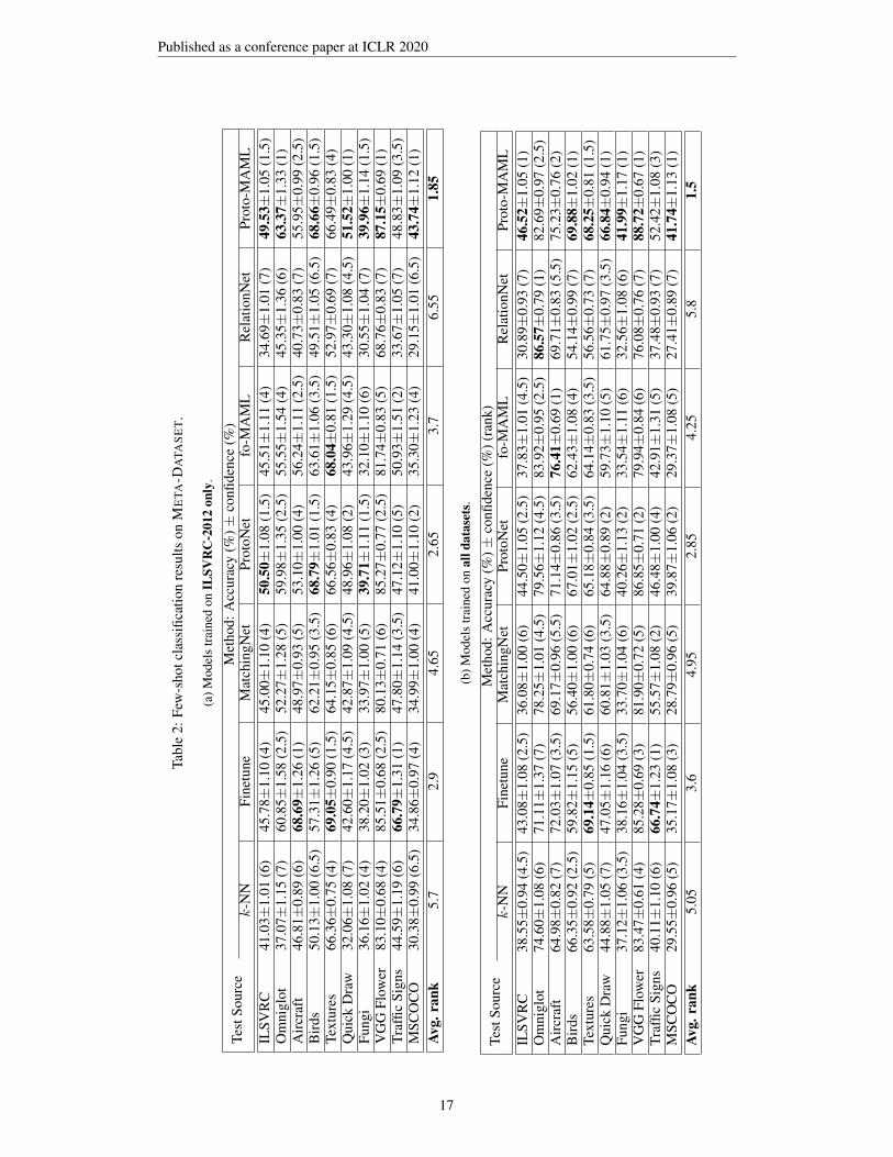
Rank computation We rank models by decreasing order of accuracy and handle ties by assigningtied models the average of their ranks. A tie between two models occurs when a 95% confidenceinterval statistical test on the difference between their mean accuracies is inconclusive in rejecting thenull hypothesis that this difference is 0. Our recommendation is that this test is ran to determine ifties occur. As mentioned earlier, our source code will include this computation.
Complete main tables For completeness, Table 2 presents a more detailed version of Table 1 thatalso displays confidence intervals and per-dataset ranks computed using the above procedure.
.6 ANALYSIS OF PERFORMANCE ACROSS SHOTS AND WAYS
For completeness, in Figure 5 we show the results of the analysis of the robustness to different waysand shots for the variants of the models that were trained on all datasets. We observe the same trendsas discussed in our Experiments section for the variants of the models that were trained on ImageNet.
10 20 30 40 50Way
0.0
0.2
0.4
0.6
0.8
1.0
Acc
ura
cy
k-NN baseline
Finetune baseline
MatchingNet
ProtoNet
fo-MAML
RelationNet
fo-Proto-MAML
(a) Ways Analysis
0 20 40 60 80 100Shot
0.0
0.2
0.4
0.6
0.8
Cla
ss P
reci
sion
k-NN baseline
Finetune baseline
MatchingNet
ProtoNet
fo-MAML
RelationNet
fo-Proto-MAML
(b) Shots Analysis
Figure 5: Analysis of performance as a function of the episode’s way, shots for models whosetraining source is (the training data of) all datasets. The bands display 95% confidence intervals.
.7 EFFECT OF TRAINING ON ALL DATASETS OVER TRAINING ON ILSVRC-2012 ONLY
For more clearly observing whether training on all datasets leads to improved generalization overtraining on ImageNet only, Figure 6 shows side-to-side the performance of each model trained onILSVRC only vs. all datasets. The difference between the performance of the all-dataset trainedmodels versus the ImageNet-only trained ones is also visualized in Figure 1 in the main paper.
As discussed in the main paper, we notice that we do not always observe a clear generalizationadvantage in training from a wider collection of image datasets. While some of the datasets that wereadded to the meta-training phase did see an improvement across all models, in particular for Omniglotand Quick Draw, this was not true across the board. In fact, in certain cases the performance isslightly worse. We believe that more successfully leveraging diverse sources of data is an interestingopen research problem.
16
Published as a conference paper at ICLR 2020
Tabl
e2:
Few
-sho
tcla
ssifi
catio
nre
sults
onM
ETA
-DA
TAS
ET
.
(a)M
odel
str
aine
don
ILSV
RC
-201
2on
ly.
Test
Sour
ceM
etho
d:A
ccur
acy
(%)±
confi
denc
e(%
)k
-NN
Fine
tune
Mat
chin
gNet
Prot
oNet
fo-M
AM
LR
elat
ionN
etPr
oto-
MA
ML
ILSV
RC
41.0
3±1.
01(6
)45
.78±
1.10
(4)
45.0
0±1.
10(4
)50
.50±
1.08
(1.5
)45
.51±
1.11
(4)
34.6
9±1.
01(7
)49
.53±
1.05
(1.5
)O
mni
glot
37.0
7±1.
15(7
)60
.85±
1.58
(2.5
)52
.27±
1.28
(5)
59.9
8±1.
35(2
.5)
55.5
5±1.
54(4
)45
.35±
1.36
(6)
63.3
7±1.
33(1
)A
ircr
aft
46.8
1±0.
89(6
)68
.69±
1.26
(1)
48.9
7±0.
93(5
)53
.10±
1.00
(4)
56.2
4±1.
11(2
.5)
40.7
3±0.
83(7
)55
.95±
0.99
(2.5
)B
irds
50.1
3±1.
00(6
.5)
57.3
1±1.
26(5
)62
.21±
0.95
(3.5
)68
.79±
1.01
(1.5
)63
.61±
1.06
(3.5
)49
.51±
1.05
(6.5
)68
.66±
0.96
(1.5
)Te
xtur
es66
.36±
0.75
(4)
69.0
5±0.
90(1
.5)
64.1
5±0.
85(6
)66
.56±
0.83
(4)
68.0
4±0.
81(1
.5)
52.9
7±0.
69(7
)66
.49±
0.83
(4)
Qui
ckD
raw
32.0
6±1.
08(7
)42
.60±
1.17
(4.5
)42
.87±
1.09
(4.5
)48
.96±
1.08
(2)
43.9
6±1.
29(4
.5)
43.3
0±1.
08(4
.5)
51.5
2±1.
00(1
)Fu
ngi
36.1
6±1.
02(4
)38
.20±
1.02
(3)
33.9
7±1.
00(5
)39
.71±
1.11
(1.5
)32
.10±
1.10
(6)
30.5
5±1.
04(7
)39
.96±
1.14
(1.5
)V
GG
Flow
er83
.10±
0.68
(4)
85.5
1±0.
68(2
.5)
80.1
3±0.
71(6
)85
.27±
0.77
(2.5
)81
.74±
0.83
(5)
68.7
6±0.
83(7
)87
.15±
0.69
(1)
Traf
ficSi
gns
44.5
9±1.
19(6
)66
.79±
1.31
(1)
47.8
0±1.
14(3
.5)
47.1
2±1.
10(5
)50
.93±
1.51
(2)
33.6
7±1.
05(7
)48
.83±
1.09
(3.5
)M
SCO
CO
30.3
8±0.
99(6
.5)
34.8
6±0.
97(4
)34
.99±
1.00
(4)
41.0
0±1.
10(2
)35
.30±
1.23
(4)
29.1
5±1.
01(6
.5)
43.7
4±1.
12(1
)Av
g.ra
nk5.
72.
94.
652.
653.
76.
551.
85
(b)M
odel
str
aine
don
alld
atas
ets.
Test
Sour
ceM
etho
d:A
ccur
acy
(%)±
confi
denc
e(%
)(ra
nk)
k-N
NFi
netu
neM
atch
ingN
etPr
otoN
etfo
-MA
ML
Rel
atio
nNet
Prot
o-M
AM
LIL
SVR
C38
.55±
0.94
(4.5
)43
.08±
1.08
(2.5
)36
.08±
1.00
(6)
44.5
0±1.
05(2
.5)
37.8
3±1.
01(4
.5)
30.8
9±0.
93(7
)46
.52±
1.05
(1)
Om
nigl
ot74
.60±
1.08
(6)
71.1
1±1.
37(7
)78
.25±
1.01
(4.5
)79
.56±
1.12
(4.5
)83
.92±
0.95
(2.5
)86
.57±
0.79
(1)
82.6
9±0.
97(2
.5)
Air
craf
t64
.98±
0.82
(7)
72.0
3±1.
07(3
.5)
69.1
7±0.
96(5
.5)
71.1
4±0.
86(3
.5)
76.4
1±0.
69(1
)69
.71±
0.83
(5.5
)75
.23±
0.76
(2)
Bir
ds66
.35±
0.92
(2.5
)59
.82±
1.15
(5)
56.4
0±1.
00(6
)67
.01±
1.02
(2.5
)62
.43±
1.08
(4)
54.1
4±0.
99(7
)69
.88±
1.02
(1)
Text
ures
63.5
8±0.
79(5
)69
.14±
0.85
(1.5
)61
.80±
0.74
(6)
65.1
8±0.
84(3
.5)
64.1
4±0.
83(3
.5)
56.5
6±0.
73(7
)68
.25±
0.81
(1.5
)Q
uick
Dra
w44
.88±
1.05
(7)
47.0
5±1.
16(6
)60
.81±
1.03
(3.5
)64
.88±
0.89
(2)
59.7
3±1.
10(5
)61
.75±
0.97
(3.5
)66
.84±
0.94
(1)
Fung
i37
.12±
1.06
(3.5
)38
.16±
1.04
(3.5
)33
.70±
1.04
(6)
40.2
6±1.
13(2
)33
.54±
1.11
(6)
32.5
6±1.
08(6
)41
.99±
1.17
(1)
VG
GFl
ower
83.4
7±0.
61(4
)85
.28±
0.69
(3)
81.9
0±0.
72(5
)86
.85±
0.71
(2)
79.9
4±0.
84(6
)76
.08±
0.76
(7)
88.7
2±0.
67(1
)Tr
affic
Sign
s40
.11±
1.10
(6)
66.7
4±1.
23(1
)55
.57±
1.08
(2)
46.4
8±1.
00(4
)42
.91±
1.31
(5)
37.4
8±0.
93(7
)52
.42±
1.08
(3)
MSC
OC
O29
.55±
0.96
(5)
35.1
7±1.
08(3
)28
.79±
0.96
(5)
39.8
7±1.
06(2
)29
.37±
1.08
(5)
27.4
1±0.
89(7
)41
.74±
1.13
(1)
Avg.
rank
5.05
3.6
4.95
2.85
4.25
5.8
1.5
17

Published as a conference paper at ICLR 2020
Figure 6: Accuracy on the test datasets, when training on ILSVRC only or All datasets (same resultsas shown in the main tables). The bars display 95% confidence intervals.
0102030405060708090 ILSVRC Omniglot Aircraft CU Birds Textures
Modelk-NN baseline
Finetune baseline
MatchingNet
ProtoNet
fo-MAML
RelationNet
fo-Proto-MAML
0102030405060708090 Quick Draw Fungi VGG Flower Traffic Sign MSCOCO
Train SourceILSVRC-2012
All datasets
.8 EFFECT OF PRE-TRAINING VERSUS TRAINING FROM SCRATCH
For each meta-learner, we selected the best model (based on validation on ImageNet’s validationsplit) out of the ones that used the pre-trained initialization, and the best out of the ones that trainedfrom scratch. We then ran the evaluation of each on (the test split of) all datasets in order to quantifyhow beneficial this pre-trained initialization is. We performed this experiment twice: for the modelsthat are trained on ImageNet only and for the models that are trained on (the training splits of) alldatasets.
The results of this investigation were reported in the main paper in Figure 3a and Figure 3b, forImageNet-only training and all dataset training, respectively. We show the same results in Figure 7,printed larger to facilitate viewing of error bars. For easier comparison, we also plot the difference inperformance of the models that were pre-trained over the ones that weren’t, in Figures 8a and 8b.These figures make it easier to spot that while using the pre-trained solution usually helps for datasetsthat are visually not too different from ImageNet, it may hurt for datasets that are significantly differentfrom it, such as Omniglot, Quickdraw (and surprisingly Aircraft). Note that these three datasetsare the same three that we found benefit from training on All datasets instead of ImageNet-only. Itappears that using the pre-trained solution biases the final solution to specialize on ImageNet-likedatasets.
.9 EFFECT OF META-LEARNING VERSUS INFERENCE-ONLY
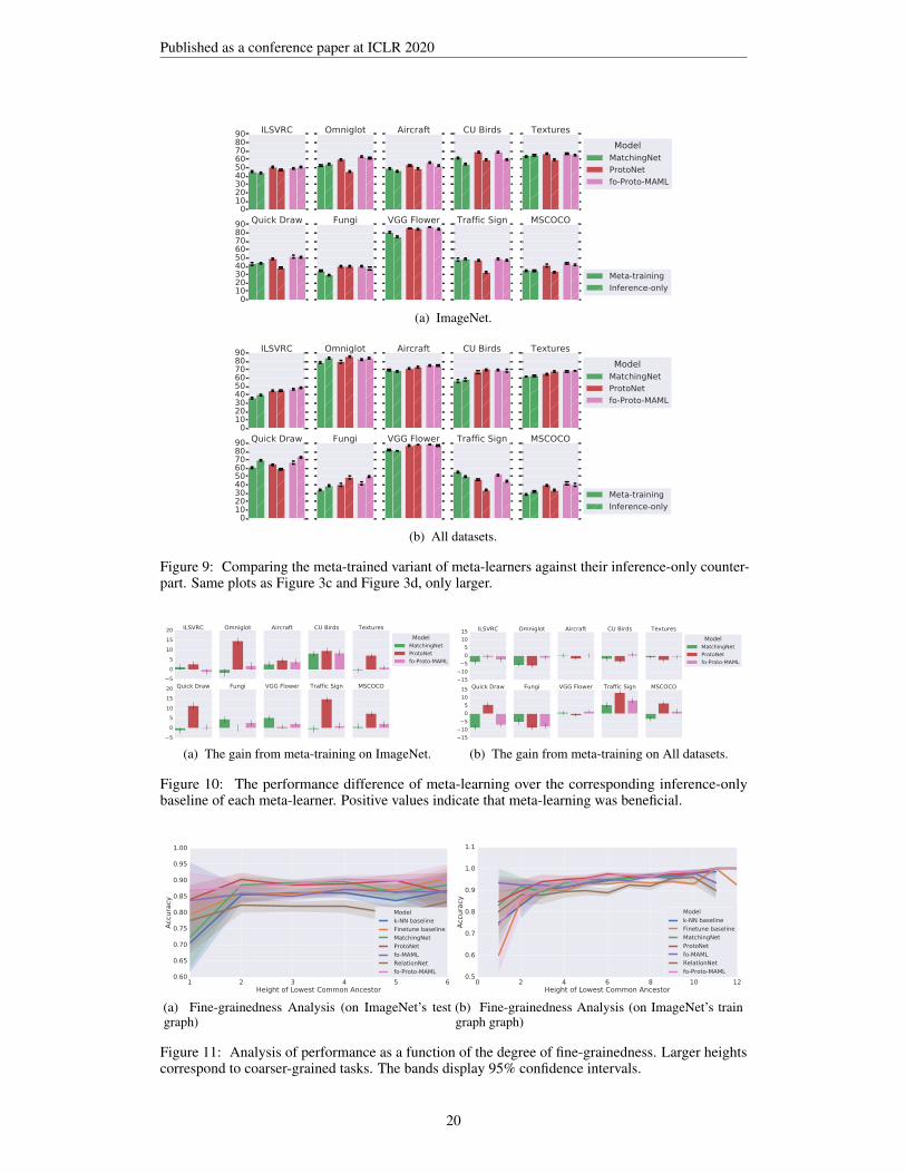
Figure 9 shows the same plots as in Figures 3c and 3d but printed larger to facilitate viewing oferror bars. Furthermore, as we have done for visualizing the observed gain of pre-training, we alsopresent in Figures 10a and 10b the gain observed from meta-learning as opposed to training thecorresponding inference-only baseline, as explained in the Experiments section of the main paper.This visulization makes it clear that while meta-training usually helps on ImageNet (or doesn’t hurttoo much), it sometimes hurts when it is performed on all datasets, emphasizing the need for furtherresearch into best practices of meta-learning across heterogeneous sources.
.10 FINEGRAINEDNESS ANALYSIS
We investigate the hypothesis that finer-grained tasks are more challenging than coarse-grained onesby creating binary ImageNet episodes with the two classes chosen uniformly at random from theDAG’s set of leaves. We then define the degree of coarse-grainedness of a task as the height ofthe lowest common ancestor of the two chosen leaves, where the height is defined as the length ofthe longest path from the lowest common ancestor to one of the selected leaves. Larger heightsthen correspond to coarser-grained tasks. We present these results in Figure 11. We do not detect asignificant trend when performing this analysis on the test DAG. The results on the training DAG,
18

Published as a conference paper at ICLR 2020
0102030405060708090 ILSVRC Omniglot Aircraft CU Birds Textures
ModelMatchingNet
ProtoNet
fo-MAML
RelationNet
fo-Proto-MAML
0102030405060708090 Quick Draw Fungi VGG Flower Traffic Sign MSCOCO
InitializationPre-trained
From scratch
(a) ImageNet.
0
20
40
60
80
100 ILSVRC Omniglot Aircraft CU Birds Textures
ModelMatchingNet
ProtoNet
fo-MAML
RelationNet
fo-Proto-MAML
0
20
40
60
80
100 Quick Draw Fungi VGG Flower Traffic Sign MSCOCO
InitializationPre-trained
From scratch
(b) All datasets.
Figure 7: Comparing pre-training to starting from scratch. Same plots as Figure 3a and Figure 3b,only larger.
1510
505
1015202530 ILSVRC Omniglot Aircraft CU Birds Textures
ModelMatchingNet
ProtoNet
fo-MAML
RelationNet
fo-Proto-MAML
1510
505
1015202530 Quick Draw Fungi VGG Flower Traffic Sign MSCOCO
(a) The gain from pre-training (ImageNet).
20
10
0
10
20
30
40 ILSVRC Omniglot Aircraft CU Birds Textures
ModelMatchingNet
ProtoNet
fo-MAML
RelationNet
fo-Proto-MAML
20
10
0
10
20
30
40 Quick Draw Fungi VGG Flower Traffic Sign MSCOCO
(b) The gain from pre-training (All datasets).
Figure 8: The performance difference of initializing the embedding weights from a pre-trainedsolution, before episodically training on ImageNet or all datasets, over using a random initializationof those weights. The pre-trained weights that we consider are the ones that the k-NN baselineconverged to when it was trained on ImageNet. Positive values indicate that this pre-training wasbeneficial.
19
Published as a conference paper at ICLR 2020
0102030405060708090 ILSVRC Omniglot Aircraft CU Birds Textures
ModelMatchingNet
ProtoNet
fo-Proto-MAML
0102030405060708090 Quick Draw Fungi VGG Flower Traffic Sign MSCOCO
Meta-training
Inference-only
(a) ImageNet.
0102030405060708090 ILSVRC Omniglot Aircraft CU Birds Textures
ModelMatchingNet
ProtoNet
fo-Proto-MAML
0102030405060708090 Quick Draw Fungi VGG Flower Traffic Sign MSCOCO
Meta-training
Inference-only
(b) All datasets.
Figure 9: Comparing the meta-trained variant of meta-learners against their inference-only counter-part. Same plots as Figure 3c and Figure 3d, only larger.
5
0
5
10
15
20 ILSVRC Omniglot Aircraft CU Birds Textures
ModelMatchingNet
ProtoNet
fo-Proto-MAML
5
0
5
10
15
20 Quick Draw Fungi VGG Flower Traffic Sign MSCOCO
(a) The gain from meta-training on ImageNet.
15
10
5
0
5
10
15 ILSVRC Omniglot Aircraft CU Birds Textures
ModelMatchingNet
ProtoNet
fo-Proto-MAML
15
10
5
0
5
10
15 Quick Draw Fungi VGG Flower Traffic Sign MSCOCO
(b) The gain from meta-training on All datasets.
Figure 10: The performance difference of meta-learning over the corresponding inference-onlybaseline of each meta-learner. Positive values indicate that meta-learning was beneficial.
1 2 3 4 5 6Height of Lowest Common Ancestor
0.60
0.65
0.70
0.75
0.80
0.85
0.90
0.95
1.00
Acc
ura
cy
Model
k-NN baseline
Finetune baseline
MatchingNet
ProtoNet
fo-MAML
RelationNet
fo-Proto-MAML
(a) Fine-grainedness Analysis (on ImageNet’s testgraph)
0 2 4 6 8 10 12Height of Lowest Common Ancestor
0.5
0.6
0.7
0.8
0.9
1.0
1.1
Acc
ura
cy
Model
k-NN baseline
Finetune baseline
MatchingNet
ProtoNet
fo-MAML
RelationNet
fo-Proto-MAML
(b) Fine-grainedness Analysis (on ImageNet’s traingraph graph)
Figure 11: Analysis of performance as a function of the degree of fine-grainedness. Larger heightscorrespond to coarser-grained tasks. The bands display 95% confidence intervals.
20

Published as a conference paper at ICLR 2020
Table 3: Improvement of fo-MAML when using a larger inner learning rate α.
(a) Models trained on ILSVRC-2012 only.
Test Source Method: Accuracy (%) ± confidence (%)fo-MAML α = 0.01 (old) fo-MAML α ≈ 0.1
ILSVRC 36.09±1.01 45.51±1.11Omniglot 38.67±1.39 55.55±1.54Aircraft 34.50±0.90 56.24±1.11Birds 49.10±1.18 63.61±1.06Textures 56.50±0.80 68.04±0.81Quick Draw 27.24±1.24 43.96±1.29Fungi 23.50±1.00 32.10±1.10VGG Flower 66.42±0.96 81.74±0.83Traffic Signs 33.23±1.34 50.93±1.51MSCOCO 27.52±1.11 35.30±1.23
(b) Models trained on all datasets.
Test Source Method: Accuracy (%) ± confidence (%)fo-MAML α = 0.01 (old) fo-MAML α ≈ 0.1
ILSVRC 32.36±1.02 37.83±1.01Omniglot 71.91±1.20 83.92±0.95Aircraft 52.76±0.90 76.41±0.69Birds 47.24±1.14 62.43±1.08Textures 56.66±0.74 64.16±0.83Quick Draw 50.50±1.19 59.73±1.10Fungi 21.02±0.99 33.54±1.11VGG Flower 70.93±0.99 79.94±0.84Traffic Signs 34.18±1.26 42.91±1.31MSCOCO 24.05±1.10 29.37±1.08
though, do seem to indicate that our hypothesis holds to some extent. We conjecture that this may bedue to the richer structure of the training DAG, but we encourage further investigation.
.11 THE IMPORTANCE OF MAML’S INNER-LOOP LEARNING RATE HYPERPARAMETER.
The camera-ready version includes updated results for MAML and Proto-MAML following anexternal suggestion to experiment with larger values for the inner-loop learning rate α of MAML.We found that re-doing our hyperparameter search with a revised range that includes larger α valuessignificantly improved fo-MAML’s performance on META-DATASET. For consistency, we appliedthe same change to fo-Proto-MAML and re-ran those experiments too.
We found that the value of this α that performs best for fo-MAML both for training on ImageNetonly and training on all datasets is approximately 0.1, which is an order of magnitude larger than ourprevious best value. Interestingly, fo-Proto-MAML does not choose such a large α value, with bestα being 0.0054 when training on ImageNet only and 0.02 when training on all datasets. Plausiblythis difference can be attributed to the better initialization of Proto-MAML which requires a lessaggressive optimization for the adaptation to each new task. This hypothesis is also supported by thefact that fo-Proto-MAML chooses to take fewer adaptation steps than fo-MAML does. The completeset of best discovered hyperparameters is available in our public code.
To emphasize the importance of properly tuning this hyperparameter, Table 3 displays the previousbest and the new best fo-MAML results side-by-side, showcasing the large performance gap whenusing the appropriate value for α.
21
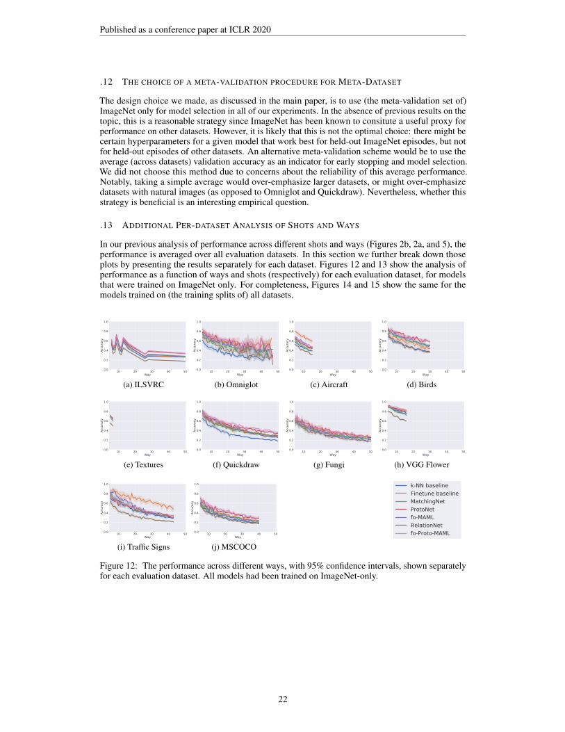
Published as a conference paper at ICLR 2020
.12 THE CHOICE OF A META-VALIDATION PROCEDURE FOR META-DATASET
The design choice we made, as discussed in the main paper, is to use (the meta-validation set of)ImageNet only for model selection in all of our experiments. In the absence of previous results on thetopic, this is a reasonable strategy since ImageNet has been known to consitute a useful proxy forperformance on other datasets. However, it is likely that this is not the optimal choice: there might becertain hyperparameters for a given model that work best for held-out ImageNet episodes, but notfor held-out episodes of other datasets. An alternative meta-validation scheme would be to use theaverage (across datasets) validation accuracy as an indicator for early stopping and model selection.We did not choose this method due to concerns about the reliability of this average performance.Notably, taking a simple average would over-emphasize larger datasets, or might over-emphasizedatasets with natural images (as opposed to Omniglot and Quickdraw). Nevertheless, whether thisstrategy is beneficial is an interesting empirical question.
.13 ADDITIONAL PER-DATASET ANALYSIS OF SHOTS AND WAYS
In our previous analysis of performance across different shots and ways (Figures 2b, 2a, and 5), theperformance is averaged over all evaluation datasets. In this section we further break down thoseplots by presenting the results separately for each dataset. Figures 12 and 13 show the analysis ofperformance as a function of ways and shots (respectively) for each evaluation dataset, for modelsthat were trained on ImageNet only. For completeness, Figures 14 and 15 show the same for themodels trained on (the training splits of) all datasets.
10 20 30 40 50Way
0.0
0.2
0.4
0.6
0.8
1.0
Accu
racy
(a) ILSVRC
10 20 30 40 50Way
0.0
0.2
0.4
0.6
0.8
1.0
Accu
racy
(b) Omniglot
10 20 30 40 50Way
0.0
0.2
0.4
0.6
0.8
1.0
Accu
racy
(c) Aircraft
10 20 30 40 50Way
0.0
0.2
0.4
0.6
0.8
1.0
Accu
racy
(d) Birds
10 20 30 40 50Way
0.0
0.2
0.4
0.6
0.8
1.0
Accu
racy
(e) Textures
10 20 30 40 50Way
0.0
0.2
0.4
0.6
0.8
1.0
Accu
racy
(f) Quickdraw
10 20 30 40 50Way
0.0
0.2
0.4
0.6
0.8
1.0
Accu
racy
(g) Fungi
10 20 30 40 50Way
0.0
0.2
0.4
0.6
0.8
1.0
Accu
racy
(h) VGG Flower
10 20 30 40 50Way
0.0
0.2
0.4
0.6
0.8
1.0
Accu
racy
(i) Traffic Signs
10 20 30 40 50Way
0.0
0.2
0.4
0.6
0.8
1.0
Accu
racy
(j) MSCOCO
k-NN baselineFinetune baselineMatchingNetProtoNetfo-MAMLRelationNetfo-Proto-MAML
Figure 12: The performance across different ways, with 95% confidence intervals, shown separatelyfor each evaluation dataset. All models had been trained on ImageNet-only.
22
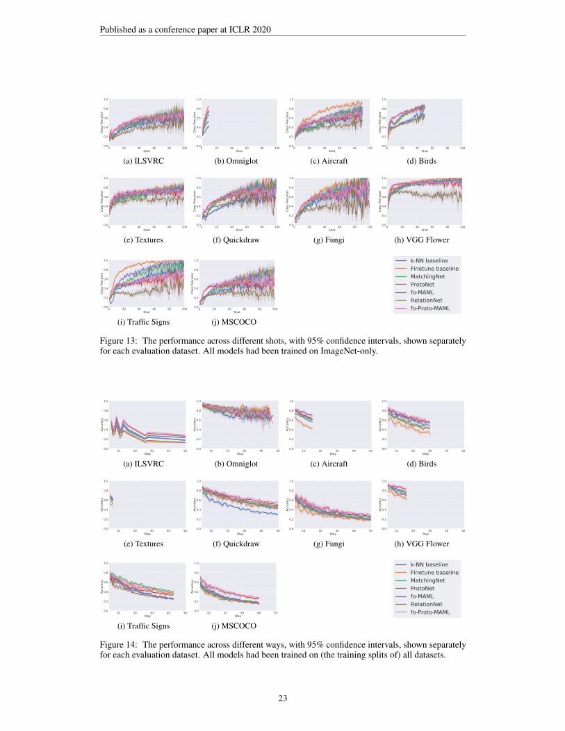
Published as a conference paper at ICLR 2020
0 20 40 60 80 100Shot
0.0
0.2
0.4
0.6
0.8
1.0Cl
ass P
recis
ion
(a) ILSVRC
0 20 40 60 80 100Shot
0.0
0.2
0.4
0.6
0.8
1.0
Clas
s Pre
cisio
n
(b) Omniglot
0 20 40 60 80 100Shot
0.0
0.2
0.4
0.6
0.8
1.0
Clas
s Pre
cisio
n
(c) Aircraft
0 20 40 60 80 100Shot
0.0
0.2
0.4
0.6
0.8
1.0
Clas
s Pre
cisio
n
(d) Birds
0 20 40 60 80 100Shot
0.0
0.2
0.4
0.6
0.8
1.0
Clas
s Pre
cisio
n
(e) Textures
0 20 40 60 80 100Shot
0.0
0.2
0.4
0.6
0.8
1.0
Clas
s Pre
cisio
n
(f) Quickdraw
0 20 40 60 80 100Shot
0.0
0.2
0.4
0.6
0.8
1.0
Clas
s Pre
cisio
n
(g) Fungi
0 20 40 60 80 100Shot
0.0
0.2
0.4
0.6
0.8
1.0
Clas
s Pre
cisio
n
(h) VGG Flower
0 20 40 60 80 100Shot
0.0
0.2
0.4
0.6
0.8
1.0
Clas
s Pre
cisio
n
(i) Traffic Signs
0 20 40 60 80 100Shot
0.0
0.2
0.4
0.6
0.8
1.0
Clas
s Pre
cisio
n
(j) MSCOCO
k-NN baselineFinetune baselineMatchingNetProtoNetfo-MAMLRelationNetfo-Proto-MAML
Figure 13: The performance across different shots, with 95% confidence intervals, shown separatelyfor each evaluation dataset. All models had been trained on ImageNet-only.
10 20 30 40 50Way
0.0
0.2
0.4
0.6
0.8
1.0
Accu
racy
(a) ILSVRC
10 20 30 40 50Way
0.0
0.2
0.4
0.6
0.8
1.0
Accu
racy
(b) Omniglot
10 20 30 40 50Way
0.0
0.2
0.4
0.6
0.8
1.0
Accu
racy
(c) Aircraft
10 20 30 40 50Way
0.0
0.2
0.4
0.6
0.8
1.0
Accu
racy
(d) Birds
10 20 30 40 50Way
0.0
0.2
0.4
0.6
0.8
1.0
Accu
racy
(e) Textures
10 20 30 40 50Way
0.0
0.2
0.4
0.6
0.8
1.0
Accu
racy
(f) Quickdraw
10 20 30 40 50Way
0.0
0.2
0.4
0.6
0.8
1.0
Accu
racy
(g) Fungi
10 20 30 40 50Way
0.0
0.2
0.4
0.6
0.8
1.0
Accu
racy
(h) VGG Flower
10 20 30 40 50Way
0.0
0.2
0.4
0.6
0.8
1.0
Accu
racy
(i) Traffic Signs
10 20 30 40 50Way
0.0
0.2
0.4
0.6
0.8
1.0
Accu
racy
(j) MSCOCO
k-NN baselineFinetune baselineMatchingNetProtoNetfo-MAMLRelationNetfo-Proto-MAML
Figure 14: The performance across different ways, with 95% confidence intervals, shown separatelyfor each evaluation dataset. All models had been trained on (the training splits of) all datasets.
23

Published as a conference paper at ICLR 2020
0 20 40 60 80 100Shot
0.0
0.2
0.4
0.6
0.8
1.0
Clas
s Pre
cisio
n
(a) ILSVRC
0 20 40 60 80 100Shot
0.0
0.2
0.4
0.6
0.8
1.0
Clas
s Pre
cisio
n
(b) Omniglot
0 20 40 60 80 100Shot
0.0
0.2
0.4
0.6
0.8
1.0
Clas
s Pre
cisio
n
(c) Aircraft
0 20 40 60 80 100Shot
0.0
0.2
0.4
0.6
0.8
1.0
Clas
s Pre
cisio
n
(d) Birds
0 20 40 60 80 100Shot
0.0
0.2
0.4
0.6
0.8
1.0
Clas
s Pre
cisio
n
(e) Textures
0 20 40 60 80 100Shot
0.0
0.2
0.4
0.6
0.8
1.0
Clas
s Pre
cisio
n
(f) Quickdraw
0 20 40 60 80 100Shot
0.0
0.2
0.4
0.6
0.8
1.0
Clas
s Pre
cisio
n
(g) Fungi
0 20 40 60 80 100Shot
0.0
0.2
0.4
0.6
0.8
1.0
Clas
s Pre
cisio
n
(h) VGG Flower
0 20 40 60 80 100Shot
0.0
0.2
0.4
0.6
0.8
1.0
Clas
s Pre
cisio
n
(i) Traffic Signs
0 20 40 60 80 100Shot
0.0
0.2
0.4
0.6
0.8
1.0
Clas
s Pre
cisio
n
(j) MSCOCO
k-NN baselineFinetune baselineMatchingNetProtoNetfo-MAMLRelationNetfo-Proto-MAML
Figure 15: The performance across different shots, with 95% confidence intervals, shown separatelyfor each evaluation dataset. All models had been trained on (the training splits of) all datasets.
24