meta-analysis of welfare-to-work programs for research on poverty discussion paper no. 1312-05...

Institute for Research on Poverty Discussion Paper no. 1312-05

Report on a Meta-Analysis of Welfare-to-Work Programs

David Greenberg Department of Economics

University of Maryland, Baltimore County E-mail: [email protected]

Andreas Cebulla

National Centre for Social Research London, United Kingdom

E-mail: [email protected]

Stacey Bouchet School of Social Work

University of Maryland, Baltimore County E-mail: [email protected]

December 2005 Research on the project described in this document was funded through a contract from the Administration of Children and Families at the U.S. Department of Health and Human Services to the Maryland Institute for Policy Analysis and Research, University of Maryland, Baltimore County. All the views expressed are those of the authors and do not necessarily reflect the views of the funding agency. The authors are grateful to Karl Koerper, Peter Germanis, Howard Rolston, and especially Leonard Sternbach for their very helpful comments on an earlier draft of this report. The authors would like to thank Laura Hudges and Abigail Davis for helping to assemble the database used for the analysis. IRP Publications (discussion papers, special reports, and the newsletter Focus) are available on the Internet. The IRP Web site can be accessed at the following address: http://www.irp.wisc.edu

CONTENTS

EXECUTIVE SUMMARY ........................................................................................................................... i 1 INTRODUCTION ........................................................................................................................... 1 2 BACKGROUND ............................................................................................................................. 3 2.1 Previous Related Research..................................................................................................... 3 2.2 The Database.......................................................................................................................... 6 2.3 Components of the Current Research .................................................................................. 10 3. META-ANALYSIS ....................................................................................................................... 12 3.1 Weighting............................................................................................................................. 13 3.2 Steps in Conducting the Statistical Analysis of the Program Effect Estimates.................... 15 4 FINDINGS OF THE DESCRIPTIVE ANALYSIS....................................................................... 19 4.1 Earnings ............................................................................................................................... 21 4.2 Percentage Employed........................................................................................................... 21 4.3 Amount of AFDC Payment.................................................................................................. 22 4.4 Percentage Participating in AFDC ....................................................................................... 22 4.5 Description of the Tested Interventions, Target Populations, and Sites .............................. 23 5. HYPOTHESES TESTED IN THE REGRESSION ANALYSES................................................. 26 5.1 Intervention Characteristics ................................................................................................. 26 5.2 Characteristics of the Target Population .............................................................................. 28 5.3 Socioeconomic Conditions at the Sites ................................................................................ 29 5.4 Selecting Explanatory Variables for the Regression Analysis............................................. 30 5.5 Omitted and Misspecified Variables .................................................................................... 33 6. BASIC REGRESSION FINDINGS .............................................................................................. 35 6.1 Sanctions .............................................................................................................................. 37 6.2 Job Search ............................................................................................................................ 37 6.3 Basic Education.................................................................................................................... 37 6.4 Vocational Education ........................................................................................................... 38 6.5 Work Experience.................................................................................................................. 38 6.6 Financial Incentives ............................................................................................................. 39 6.7 Time Limits.......................................................................................................................... 39 6.8 Number of Years since 1982................................................................................................ 39 6.9 One-Parent Families versus Two-Parent Families ............................................................... 40 6.10 Average Age of the Target Group........................................................................................ 40 6.11 Percentage of the Target Group Employed in the Year Prior to Random Assignment........ 41 6.12 Annual Percentage Change in Local Manufacturing Employment...................................... 41 6.13 Poverty Rate......................................................................................................................... 42 6.14 Maximum AFDC Payments................................................................................................. 43 6.15 Summary of Key Findings ................................................................................................... 43 7. SENSITIVITY ANALYSES ......................................................................................................... 44 8. THE PREDICTIVE ABILITY OF THE REGRESSIONS............................................................ 46 9. PROGRAM IMPACTS OVER TIME........................................................................................... 50 10. ANALYSIS OF OUTLIERS ......................................................................................................... 53 10.1 The Prevalence of Outlier Programs and Outlier Estimates................................................. 54 10.2 Separating Positive and Negative Outliers........................................................................... 56 10.3 What Causes Type B Outliers to Occur? ............................................................................. 59 11. ANALYSIS OF BENEFIT-COST FINDINGS ............................................................................. 60 11.1 Descriptive Analysis ............................................................................................................ 62 11.2 Regression Analysis ............................................................................................................. 64 12. ANALYSIS OF SUBGROUPS ..................................................................................................... 67 12.1 Caveats ................................................................................................................................. 69

12.2 Three Types of Analyses...................................................................................................... 70 12.3 Findings for the Comparison of Unadjusted Means for the Pure Subgroups....................... 71 12.4 Findings for Quarter 7 Differences in Means between Subgroups ...................................... 73 13. ANALYSIS OF CHILD OUTCOMES.......................................................................................... 76 13.1 Evaluations that Measured Child Outcomes ........................................................................ 78 13.2 A Meta-Analysis of Program Effects on Children ............................................................... 80 13.3 Findings................................................................................................................................ 81 13.4 Regression Findings ............................................................................................................. 83 13.5 Summary of Key Findings ................................................................................................... 84 14. VOLUNTARY PROGRAMS........................................................................................................ 85 15. SUMMARY OF FINDINGS AND CONCLUSIONS................................................................... 87 15.1 Impacts of Mandatory Welfare-to-Work Interventions ....................................................... 87 15.2 What Makes Welfare-to-Work Interventions Successful?................................................... 88 15.3 Effectiveness among Subgroups .......................................................................................... 89 15.4 Program Impacts over Time................................................................................................. 90 15.5 Analysis of Outliers.............................................................................................................. 90 15.6 Costs and Benefits................................................................................................................ 90 15.7 Child Outcomes.................................................................................................................... 91 15.8 Voluntary Programs ............................................................................................................. 92 15.9 Conclusions: Lessons for Policy and Analysis .................................................................... 92 APPENDIX A. The Welfare-to-Work Program (Meta-Analysis) Database............................................... 95 APPENDIX B. Measurement of Child Outcomes ...................................................................................... 99 APPENDIX TABLES............................................................................................................................... 101 FIGURE 1. How Welfare Policies Might Affect Children ....................................................................... 105 TABLES 1–27 .......................................................................................................................................... 107 REFERENCES ......................................................................................................................................... 139

EXECUTIVE SUMMARY

This report uses meta-analysis, a set of statistically based techniques for combining quantitative

findings from different studies, to synthesize estimates of program effects from random assignment

evaluations of welfare-to-work programs and to explore the factors that best explain differences in the

programs’ performance. The analysis is based on data extracted from the published evaluation reports and

from official sources. All the programs included in the analysis targeted recipients of Aid to Families with

Dependent Children (AFDC; now called Temporary Assistance for Needy Families, TANF1). The

objective of the analysis is to establish the principal characteristics of welfare-to-work programs that were

associated with differences in success, distinguishing between variations in the services received,

differences in the characteristics of those who participated in each program, and variations in the

socioeconomic environment in which the programs operated.

Meta-analysis is a powerful instrument for analyzing the combined impacts of comparable policy

interventions, while controlling for a range of factors pertaining to these interventions or the environment

in which they took place. However, like other statistical techniques, meta-analysis can be subject to data

limitations that adversely affect its capacity to produce robust and reliable results. Multicollinearity of

variables (resulting from small sample size), inconsistencies in the information provided in different

evaluation reports, and omitted or misspecified variables are some of the data analysis risks that we

sought to minimize by, for instance, verifying data entries and carefully considering the specification of

the regression equations that are estimated. It would have been impossible, as well as impractical, to

eradicate all risk of error in the analyses, much of which would have been beyond the control of this study

and could be traced back to the original evaluations. In the light of such limitations, many of the

1Because most data used in this study were generated before AFDC was converted to the Temporary Assistance for Needy Families program, for convenience we use the AFDC acronym throughout this report.

ii

conclusions that are reached are subjected to sensitivity tests. These tests were conducted to establish the

robustness of the meta-analyses’ key findings.

Separate meta-analyses of both voluntary and mandatory programs were conducted. Voluntary

programs provide services (e.g., help in job search, training, and remedial education) for those who apply

for them, and they sometimes provide financial incentives to encourage work. Mandatory programs are

targeted at recipients of government transfer payments. They also provide employment-oriented services

and sometimes provide financial work incentives, but differ from voluntary programs by requiring

participation in the services by potentially subjecting individuals assigned to the program to fiscal

sanctions (i.e., reductions in transfer payments) if they do not cooperate.

This study uses a unique database, assembled specifically for synthesizing findings from

evaluations of welfare-to-work programs. The data used in the study are from 27 random assignment

evaluations of mandatory welfare-to-work programs for AFDC applicants and recipients and four random

assignment evaluations of voluntary welfare-to-work programs for AFDC recipients. The evaluations in

the study sample were conducted similarly. AFDC applicants and recipients were randomly assigned to

either a program group that participated in the welfare-to-work program being evaluated or to a control

group, which was eligible to receive any services that existed prior to the introduction of the welfare-to-

work program. Relying mainly on administrative data, various measures of outcomes (such as earnings

and the percentage receiving AFDC) were computed for the members of the program and control groups

over time. Once this follow-up information was available, each program effect was estimated as the

difference in the mean outcome for the program group and the control group, a measure that is often

referred to as the “program impact.”

The database contains four measures of program impacts:

• average earnings,

• the percentage in employment,

• the average amount of AFDC received, and

iii

• the percentage in receipt of AFDC.

Program impacts are available for up to twenty calendar quarters after random assignment, along

with the levels of statistical significance for each of these impact measures. Findings from cost-benefit

analyses are also included when available. In addition, the database contains the values of a number of

explanatory variables. These include the characteristics of the program population (gender and ethnic

mix, age distribution, family structure, education levels, and so forth), measures of program effects on

participation in various activities (job search, basic education, vocational training, and work experience),

whether each evaluated program tested financial incentive and time limits, program effects on

sanctioning, and socioeconomic data for each of the program sites and for each of the evaluation years

(site unemployment and poverty rates, the percentage of the workforce in manufacturing employment,

median household income, and the maximum AFDC payment for which a family of three was eligible).

Because controls often receive services similar to those received by persons assigned to the

evaluated programs, but from other sources, it is important to measure the net difference between the two

groups in their receipt of services—that is, the program’s impact on participation in services. These net

differences indicate that a typical mandatory welfare-to-work program puts much more emphasis on

increasing participation in relatively inexpensive activities, such as job search, than on increasing

participation in more costly activities, such as basic education and vocational training. Nonetheless, it cost

the government almost $2,000 (in year 2000 dollars) more per member of the program group to operate

the evaluated mandatory programs than to run the programs serving controls. Voluntary programs

typically put more emphasis on expensive services than mandatory programs do and, hence, are usually

more costly to run.

The four impacts mentioned above were examined in four separate calendar quarters (the 3rd, 7th,

11th, and 15th after random assignment). Between 64 and 79 estimates were available for each impact

measure during the two earlier quarters, and between 44 and 56 estimates were available during the later

two quarters. The analysis suggests that welfare-to-work programs, on average, had the intended positive

iv

impact on the four indicators, although these averages were usually small. There was considerable

variation among the individual programs, however, suggesting that some performed much better than

others.

Much of the analysis was devoted to determining why some programs were more successful than

others. Among the more important conclusions concerning mandatory welfare-to-work programs that

were reached are the following (findings for voluntary programs are described later):

• Three program features appear to be positively related to the effectiveness of mandatory welfare-to-work interventions: increased participation in job search, the use of time limits, and the use of sanctions. The sanction impact is only important in the first couple of years after entry into a program.

• Financial incentives decrease impacts on whether AFDC is received and on the amount of AFDC that is received, but do not improve impacts on labor market outcomes.

• The evidence is somewhat mixed over whether increases in participation in basic education, vocational education, and work experience increase program effectiveness. However, in general the findings do not support putting additional resources into these activities.

• It is not clear whether the effectiveness of mandatory welfare-to-work programs has improved over time.

• Mandatory welfare-to-work programs appear to do better in strong labor markets than in weak ones.

• Because generous state AFDC programs (represented in the analysis by the size of the maximum AFDC payment for which a family of three is eligible) reduce incentives to leave the welfare rolls, it was anticipated that the relationship between AFDC generosity and program impacts on the receipt of AFDC would be negative. However, the evidence on this relationship is mixed, varying with the statistical procedures used to test the hypothesis.

• A typical mandatory welfare-to-work program appears to have a positive effect on all four program impact measures for five to seven years after random assignment, although the impacts begin to decline after two or three years.

• In general, mandatory welfare-to-work programs appear to be more effective in serving relatively more disadvantaged caseloads than more advantaged caseloads—for example, AFDC recipients (rather than applicants), program group members without recent employment experience (rather than program group members with recent employment experience), and long-term (rather than short-term) participants in AFDC. However, similar evidence of a differential impact for program group members with and without a high school diploma is lacking. Moreover, there is some evidence of a positive relationship between program impacts and the average age of persons in the caseload.

v

The findings listed above are based on weighted regressions in which the dependent variables are

estimates of program impacts and the weights, as prescribed by meta-analysis, are the inverse of the

standard errors of the impact estimates. The report provides evidence suggesting that these regressions

can be used to assess whether it is likely that a particular mandatory welfare-to-work program is

performing better or worse than an average mandatory program. Although this information is not as

reliable as that provided by a full evaluation, it can serve as a partial substitute for such an evaluation.

The net operating costs of a typical mandatory welfare-to-work program (i.e., the cost to the

government of providing program services, excluding income transfers, such as AFDC payments), were

around $1,800 per program group member (in year 2000 dollars). These costs, most of which are incurred

in the first few months after participants enter a program, are larger for programs that substantially

increase participation in basic education and vocational education. Increases in participation in work

experience do not seem to increase costs, perhaps because work experience participants are often assigned

to agencies other than those operating the welfare-to-work programs, and whatever costs are involved

may not get incorporated into estimates of net operating costs. Increases in participation in job search

appear to result in very small increases in cost, while financial incentives appear fairly costly to

administer. Increases in sanction rates engender considerable costs, presumably because of government

expenditures required for administering and enforcing sanctions.

Benefit-cost analyses were conducted as part of the evaluation of many, but far from all, of the

evaluations of the welfare-to-work programs in the database. Findings from these analyses indicate that

the net benefits (i.e., benefits less costs) of a typical mandatory welfare-to-work program are surprisingly

small. According to the findings, which attempt to capture total net benefits over several years (often

five), society receives net benefits of around $500 per program group member from a typical mandatory

welfare-to-work program; savings to the government are around $400 per program group member, on

average; and those assigned to a typical program are barely affected. It is likely that the net benefits from

a typical mandatory welfare-to-work program are actually even smaller than these estimates imply

vi

because, as shown in the report, benefit-cost analyses are less likely to be conducted for those programs

with especially small impacts on earnings.

Unsurprisingly, the net benefits received by participants are higher for program group members in

programs that offer financial incentives than for those assigned to programs that do not. However, the

increases in participant net benefits are fully or nearly offset by reductions in government net benefits.

Thus, the social cost of financial incentives appears to be small or negligible. Because the findings also

suggest that they do little to increase employment or earnings, financial incentives that are provided

through welfare-to-work programs are perhaps best viewed as simply transferring income from the

government to low-wage welfare recipients who find jobs.

We used meta-analysis to systematically identify interventions with very high positive or negative

impacts. In doing so, we defined “very high” positive or negative impacts as those at least one standard

deviation above or below, respectively, the mean for all interventions. We did this for all four impact

measures for quarters 3, 7, 11, and 15. We required interventions to have at least two quarterly outliers

before classifying them as having had exceptionally high positive or negative outliers because we were

interested in identifying programs that repeatedly, perhaps persistently, under- or overperformed. This

was to avoid highlighting isolated instances of above-average positive or negative performance that may

not be sustained over time. We conducted two types of analysis: (1) we compared each impact estimate in

a given calendar quarter to the weighted mean of all impact estimates available for that quarter (Type A);

(2) we used the weighted regressions and their explanatory variables to control for factors that influence

the effectiveness of welfare-to-work interventions (Type B). We find, as expected, that interventions are

more likely to produce Type A than Type B outliers. Additional analysis that may well be worth

undertaking, but that would require information beyond that in our database, would be required to

determine why interventions that produced Type B outliers were over- or underperforming.

As indicated by the fact that they produced multiple positive outliers for different impact

measures, the GAIN evaluation interventions in California’s Riverside and Butte Counties and the

vii

NEWWS evaluation in Portland Oregon are among those that repeatedly overperformed. Other

interventions with repeated positive outlier impacts include the California Work Pays Demonstration and

the New York State Child Assistance Program. Both record more Type B than Type A outliers; that is,

their status as overperforming interventions becomes more apparent after the factors that influence

program impacts have been taken into account. Repeatedly underperforming programs include

Minnesota’s Family Investment Program (MFIP), Vermont’s Welfare Restructuring Project (WRP), and

GAIN’s Tulare County intervention. MFIP especially underperformed with respect to reducing AFDC

payments or the number of AFDC recipients, perhaps because it offered financial incentives.

Seven of the random assignment evaluations of mandatory welfare-to-work programs in our

database provided sufficient information on child outcomes for analysis as part of this report. Even

though the data severely limited in-depth analysis of program impacts for children, several findings are

noteworthy. Overall, program impacts on children were small, but there is evidence that the considerable

variation across programs in their estimated impacts on children is not entirely due to sampling error, but

is partially attributable to systematic differences among the interventions. However, with the exception of

impacts on the emotional and behavioral problems of children, we were unable to determine what these

systematic differences might be.

There is no support in our data for the proposition that increasing the net incomes of welfare

families improves child outcomes. However, the welfare-to-work programs that were examined did not

produce large changes in the incomes of those assigned to them. When various program characteristics

are controlled, impacts on emotional and behavioral problems are less positive for school-age children

than for young children. Additionally, three program features appear to positively affect the impact of

welfare-to-work interventions on children’s behavioral and emotional outcomes: sanctions, participation

in basic education, and participation in unpaid work. Two features of welfare-to-work programs exert

negative influences on impacts on childhood behavioral or emotional impacts: financial incentives and

viii

time limits. Finally, increasing expenditures on welfare-to-work programs has a positive effect on their

impacts on childhood behavioral and emotional problems.

There have been four evaluations of ten interventions that paid a stipend to AFDC recipients who

volunteered for temporary jobs that were intended to help them learn work skills. These voluntary

welfare-to-work interventions increased the earnings and decreased the AFDC payments of participants

by modest, but nontrivial, amounts. However, there is fairly substantial variation in these impacts. A

partial explanation for this variation appears to be that more expensive voluntary welfare-to-work

programs produce larger impacts on earnings and AFDC payment amounts than less expensive programs.

We found no evidence of a similar relationship between program costs and program impacts for

mandatory welfare-to-work programs.

The research that is presented in this report suggests a number of conclusions about welfare-to-

work programs. One that particularly stands out is that although there are a few welfare-to-work programs

that may be worth emulating, most such programs by themselves are unlikely to reduce the size of welfare

rolls by very much or to improve the lives of most program group members and their children very

substantially. Thus, they must be coupled with other policies, such as earnings subsidies.

Report on a Meta-Analysis of Welfare-to-Work Programs

1. INTRODUCTION

The research presented in this report uses meta-analysis to conduct a statistical synthesis of

findings from random assignment evaluations of welfare-to-work programs and to explore the factors that

best explain differences in performance. The analysis is based on data extracted from the published

evaluation reports and from official sources. All the programs included in the analysis were targeted on

recipients of Aid to Families with Dependent Children (AFDC).2 The objective of the analysis is to

establish the principal characteristics of welfare-to-work programs that were associated with differences

in success, distinguishing among variations in the services received, differences in the characteristics of

those who participated in each program, and variations in the socioeconomic environment in which the

programs operated.

In part, the origins of this report can be traced back to the greater use of the “1115 waiver

authority” in the 1980s and, especially, the 1990s. Although available since the 1960s, waivers were

increasingly applied for by U.S. states that wanted to experiment with their welfare provisions, including

not only welfare-to-work programs, but also involving child support measures and Food Stamps and

Medicaid provisions. The federal government became more receptive to the idea of welfare-to-work

experimentation and increasingly granted state waivers, leading to a rapid rise in new welfare-to-work

programs being tried and tested. In exchange, states were usually required to evaluate the policy changes

they implemented, and the federal government increasingly required more rigorous evaluations that

included the use of random assignment. However, it is important to recognize that a number of states did

not have to be coaxed by the waiver process to undertake random assignment evaluations of the welfare-

2Because most data used in this study are for years before AFDC was converted to the Temporary Assistance for Needy Families (TANF) program, for convenience we use the AFDC acronym throughout this report.

2

to-work programs, but did so voluntarily because of a desire to learn about the effectiveness of their

innovations. Interestingly, the interest of both the states and the federal government in random assignment

evaluations during the 1990s was stimulated by a series of successful random assignment evaluations

undertaken in the early 1980s by MDRC, a New York City evaluation firm.

Thus, by the turn of the last century, there were a plethora of evaluations of welfare-to-work

programs designed to promote work and reduce welfare caseloads, the results of which have been widely

disseminated (Greenberg and Shroder, 2004; Friedlander, Greenberg, and Robins, 1997; Gueron and

Pauly, 1991; Greenberg and Wiseman, 1992; and Walker, 1991). The evaluations measured the effects

(usually called “impacts”) of welfare-to-work programs on outcome indicators, such as the receipt of

welfare, the employment status of welfare recipients, their earnings, and the amount of welfare benefit

they received. Some, but not all, of these evaluations also estimated the overall costs and benefits of the

evaluated programs. Some of the more recent evaluations have also measured program impacts on

measures of the welfare of the children of program participants. These impact measures are all examined

in the report.

While the evaluations were able to gauge the effectiveness of each welfare-to-work program, they

were rarely able to determine reliably the program features that contributed to success or failure. For

instance, social and environmental conditions affecting program sites were seldom taken into account, nor

were the characteristics of programs. In fact, they did not need to be, because the evaluation designs used

by many studies, based on random assignment of welfare recipients into experimental and control groups,

guaranteed that individuals in the two groups shared environmental conditions and characteristics. In

addition, evaluations often recorded impacts for only the first one, two, or three years after program

implementation and were thus unable to assess the long-term performance and viability of interventions.

Because their evaluation period was short-term, there was again less need to control for conditions that

might have affected impacts over time.

3

Meta-analysis provides a statistically based means for assembling and distilling findings from

collections of policy evaluations. The approach is based on a well-established statistical methodology. On

the basis of a comprehensive, systematic review of available evidence, meta-analysis is a check against

unwarranted generalizations and unfounded myths, and therefore can help lead to a more sophisticated

understanding of the subtleties of policy impacts.

The remainder of this report first provides additional background information, including a

discussion of previous statistical syntheses of welfare-to-work programs and a description of the specially

constructed database of welfare-to-work evaluations that is used in the study. It then outlines the

methodological principles of meta-analysis. This is followed by a discussion of findings from a formal

meta-evaluation of the welfare-to-work programs in our sample. Finally, the findings are summarized and

conclusions are drawn on their policy implications.

2. BACKGROUND

2.1 Previous Related Research

In a 1997 summary of training and employment program evaluations, Friedlander et al. suggested

that welfare-to-work programs typically result in modest, but sometimes in substantial, positive effects on

the employment and earnings of one-parent families headed by women. They also noted that the programs

are often found to reduce the receipt of welfare and welfare payment levels of these families, but these

effects are usually modest and tend to decrease over time. The evidence is less clear for two-parent

families.

Friedlander et al. (1997) make a useful distinction between voluntary and mandatory programs.

Voluntary programs provide services (e.g., help in job search, training, and remedial education) for those

who apply for them and they sometimes provide financial incentives to work for individuals who apply

for them. Mandatory programs are targeted at recipients of government transfer payments. They also

provide employment-oriented services and sometimes provide financial work incentives, but they

4

formally require participation in the services by potentially subjecting individuals assigned to the program

to fiscal sanctions (i.e., reductions in transfer payments) if they do not cooperate.

The Friedlander et al. (1997) review also indicates that there is considerable variation in the

effectiveness of different training and employment programs. As previously indicated, a key objective of

the research described in this report is to examine the extent to which this variation is attributable to the

characteristics of the programs themselves, the characteristics of participants in the programs, and the

economic environment in which the programs are conducted.

In previous, closely related, work, we conducted a meta-analysis of 24 random-assignment

evaluations of mandatory welfare-to-work programs that operated in over 50 sites between 1982 and 1996

and were targeted at one-parent families on AFDC. Published papers on this research (Ashworth et al.,

2004, and Greenberg et al., forthcoming) highlighted the effects of the receipt of program services and

participant and site characteristics on program impacts on earnings and the receipt of AFDC. For

example, the findings suggest that higher levels of program sanctioning rates result in larger impacts on

earnings and leaving the welfare rolls. They also imply that if a program can increase the number of

participants who engage in job search, it will, as a result, have larger effects on their earnings and on their

ability to leave the welfare rolls. On the other hand, increases in participation in basic or remedial

education, vocational training, or work experience and the provision of financial work incentives do not

appear to result in larger increases in earnings. Additional findings from the meta-analysis indicate that

program impacts on earnings are larger for white than for nonwhite participants and for older participants

than for younger participants. They also appear to be larger when unemployment rates are relatively low.

In another published paper, Greenberg et al. (2004) examined how program impacts on earnings change

over time and found that the effects of a typical welfare-to-work program appear to increase after random

assignment for two or three years and then disappear after five or six years.

Of all the welfare-to-work programs that have been evaluated by random assignment in the

United States, the two that operated in Riverside, California, and Portland, Oregon, produced the most

5

dramatic impacts. As a result, these programs have become very well known. Greenberg et al.

(forthcoming) examined the factors that contributed to Riverside and Portland’s exceptional success.

More specifically, they first measured the difference in impacts for these two programs and the impact for

an average site. They then determined whether the estimated regression could explain a substantial

proportion of these differences (it typically could). The findings suggest that only part of this success can

be attributed to the design of the programs that operated in Riverside and Portland. The social and ethnic

mix of the programs’ participants and the economic conditions prevailing at Riverside and Portland at the

time of evaluation were also important.

There have been several recent studies in addition to our own that have also attempted to unravel

the factors that cause program effectiveness to vary across training, employment, and welfare-to-work

programs. For example, the National Evaluation of Welfare-to-Work Strategies, which provides a

comparative analysis of eleven welfare-to-work programs over a five-year period, was particularly

concerned with comparing the effectiveness of employment-focused and education-focused programs

(Hamilton et al., 2001). However, although this study compared impacts across different programs, it did

not control for differential exogenous factors, such as variations in the mix of program participants or in

economic conditions. It found that welfare-to-work programs that emphasize labor market attachment

were more effective in reducing welfare spending, increasing earnings, and facilitating the return to

employment of participants than programs that emphasized human capital development.

In a path-breaking re-analysis of random assignment evaluations of California’s Greater Avenues

for Independence (GAIN) program, Florida’s Project Independence, and the National Evaluation of

Welfare-to-Work Strategies, Bloom, Hill, and Riccio (2003) pooled the original survey data for over

69,000 members of program and control groups who were located in 59 different welfare offices. The

resulting hierarchical linear analysis, which utilized unpublished qualitative data on the program delivery

processes, found that the way in which welfare-to-work programs were delivered and the emphasis that

was placed on getting the “work-first” message across strongly affected the second-year impacts of the

6

programs included in the analysis. The results also indicated that welfare-to-work programs were less

effective in environments with higher unemployment rates.

Greenberg, Michalopoulos, and Robins (2003) have recently completed a meta-analysis of the

impacts of voluntary training programs on earnings. They systematically took account of differences in

program design, the characteristics of program participants, and labor market conditions. Their analysis

indicates that program effects are greatest for adult women participants (many of whom received

welfare), modest for adult men, and negligible for youth. They also found race to be an important

determinant of program impacts on earnings and that, at least for adults, more expensive programs were

not more effective than otherwise similar less expensive programs.

2.2 The Database

All the studies listed above provide useful information. However, the database on which we based

our previous research offered several distinct advantages over the data sources utilized in the other

studies. In particular, the database:

1. Provided the widest coverage of mandatory welfare-to-work program evaluations by including all those available by the end of 2000 that used a random assignment design to assess programs that provided job search, training services, or financial incentives to encourage work to AFDC recipients. However, unlike Hamilton et al. (2001) and Bloom, Hill, and Riccio (2003), it utilized data that pertain to each evaluated program (“macro-level” data), not to individual members of program and control groups (“micro-level” data).

2. Recorded all the quarterly and annual program impact estimates that were published in various reports from these evaluations by the end of 2000.

3. Included variables that pertain to the receipt of program services, the characteristics of program participants, and the characteristics of the sites in which the programs operated.

The database that we previously used for the studies described above has been greatly updated

and expanded for use in the research described in this report. First, data for new impact estimates for

previously evaluated mandatory welfare-to-work programs have been added. Second, data from several

more recently initiated random-assignment evaluations of mandatory welfare-to-work programs have also

been incorporated into the database. Third, the database that we previously used contained information on

7

only mandatory welfare-to-work programs. Random-assignment evaluations of voluntary programs that

were targeted specifically at AFDC recipients have now been added. Fourth, indicators of the evaluated

programs’ impact on the well-being of the children of program participants, as well as outcome

information on the children of controls, have been added to the database for those programs for which

they are available. Fifth, the original database recorded the net effect of mandatory welfare-to-work

programs on the proportion of program participants who were sanctioned (that is, it indicates the

experimental-control difference in percentage sanctioned) and indicated whether each evaluated program

provided financial work incentives. The information in the database about sanctions and financial

incentives has been greatly expanded. For example, it now records the duration of the sanctions and

whether the sanctions required the complete or only the partial withdrawal of AFDC benefits. For those

evaluated programs that offered financial work incentives to welfare recipients, the database now

indicates the dollar amount of the financial incentive that would be received by an individual with two

children who has been in a full-time minimum wage job for two months. A similar calculation is available

for an individual who has worked full-time for 13 months. All financial information that is recorded in the

database—and, by implication, available for use in this report—has been inflated to year 2000 dollars.

Further information about the database and how it can be accessed is provided in Appendix A.

The random assignment welfare-to-work evaluations that are included in the database are listed in

Table 1.3 Some of the listed evaluations were conducted at more than one site. Moreover, some of these

sites experimented with more than one type of welfare-to-work program (or intervention). In other words,

3Four of the evaluations listed in Table 1 are excluded from the meta-analysis described in this report. Two of the evaluations were of a voluntary pilot program that was run in Canada, the Self-Sufficiency Project (SSP). Because of differences in the Canadian and U.S. welfare systems, as well as other differences between the two countries, in conducting a meta-analysis, data from the SSP evaluations should probably not be pooled with evaluation data from the United States, and we did not do so. Another excluded program is New York State’s Comprehensive Employment Opportunities Support Centers Program. This voluntary program was simply unique; there was no other program to which it could be appropriately compared. The final excluded evaluation is of the Wisconsin Self-Sufficiency First/Pay for Performance Program, a mandatory program. This evaluation was subject

8

an evaluation may have reported the impacts of several interventions, undertaken at several sites. This is

reflected in our database, which records the impacts for each site and intervention separately. For

example, the National Evaluation of Welfare-to-Work Strategies (NEWWS) pertains to 11 interventions

at seven sites.

The majority of the evaluations of mandatory welfare-to-work programs in our database were

conducted in the 1990s. For 77 of the 116 interventions recorded in the database, random assignment

commenced between 1990 and 1998. A further 38 interventions were evaluated in the 1980s, including a

few for which the random assignment extended into the following decade. One evaluation, MDRC’s

study of the National Supported Work Demonstration program, was completed in the 1970s. Only one

evaluation, Indiana’s Welfare Reform program, was conducted after the introduction of TANF, which

replaced AFDC4 and took effect July 1, 1997.5 TANF ended federal entitlement to assistance and created

block grants to fund state expenditures on benefits, administration, and services to needy families. It also

introduced time limits on the receipt of welfare assistance and changed work requirements for benefit

recipients. 6

to a number of technical problems and, consequently, only limited confidence can be placed in the estimates of program effects that were produced by it.

4It also replaced the Job Opportunities and Basic Skills Training (JOBS) program and the Emergency Assistance (EA) program.

5Indiana’s Welfare Reform program included the random assignment of two participant and control group cohorts. The assignment for the later cohort commenced in March 1998 and was completed in February 1999. In all other cases, the random assignment process had started and was completed before TANF took effect. Five of the evaluated state welfare reform programs listed in Table 1 continue to run under the same name at the time of writing (May 2005), although some may have modified their service contents. These are California’s CALWORKS, Delaware’s A Better Chance (ABC), Iowa’s Family Investment Program (FIP), Minnesota’s Family Investment Program (MFIP) and Virginia’s Initiative for Employment, not Welfare (VIEW).

6The introduction of TANF in lieu of AFDC was intended to enhance the services available to welfare recipients and improve their effectiveness in placing recipients in jobs, increasing their earnings, and reducing their welfare dependency. It is conceivable, therefore, that the taking effect of TANF would influence some of our findings. As explained in more detail below, we conduct the meta-analysis for different calendar quarters after the random assignment of program and control groups. For those interventions that completed random assignment in the mid-1990s, impacts that were measured three or four years after random assignment, in fact, occurred after the date during which TANF took effect. It is impossible to determine with precision the number of persons assigned to the samples used in the evaluations in our database that may have been affected by TANF because program evaluations

9

All the evaluated welfare-to-work programs listed in Table 1 were intended to encourage

employment and also, in most cases, to reduce dependency on welfare. The evaluations are divided

between those that assessed mandatory programs and those that examined voluntary programs. There are

a few evaluations listed in Table 1 that assessed programs that provided financial work incentives but not

services. We classify those “pure” financial work incentive programs for which individuals had to apply

as “voluntary” and those for which welfare recipients were made eligible, regardless of whether they

applied, as “mandatory.” Individuals assigned to “pure” financial work incentive programs that are

classified as “mandatory” were obviously not subject to sanctions for refusal to participate in services, as

no services were offered. However, the manner in which eligibility to participate in the program was

determined was similar to that of mandatory programs that did provide services.

The older experiments listed in Table1 (for example, SWIM in San Diego and the Employment

Initiatives program in Baltimore) tended to be of demonstration programs, which were run for the express

purpose of seeing how well they functioned. The study sites volunteered for this purpose and may not

have been very representative. For example, funding levels may have been high and the staff

exceptionally motivated. However, there is little evidence on whether the findings were distorted by such

factors. Most of the more recent random assignment evaluations (for example, the Virginia Independence

Program and the Indiana Welfare Reform program) resulted because a state desired to implement a new

program and as a condition of obtaining federal waivers was required to evaluate the intervention using

random assignment. These evaluations often took place when state AFDC programs were undergoing

typically do not provide data about the number of individuals randomly assigned at each point in time during the random assignment process. However, assuming a steady process of random assignment with a similar number of individuals assigned in each calendar quarter, we estimate that, in the case of the 3rd quarter impact measurements in our database, roughly 1 percent were taken during or after 1997. This increased to around 6 percent for Quarter 7, 16 percent for Quarter 11, and 42 percent for Quarter 15. (We count an impact measurement as having taken place during or after 1997 if the evaluation data for at least half the sample population pertain to that period. See also footnote 13.) Our analysis captures some of the potential effect of TANF by including an independent variable that measures for each evaluation the years between its mid-point of random assignment and the mid-point of random assignment of the earliest of the evaluation, included in our database.

10

many changes. Consequently, staff was probably less motivated and had less time to focus on the

innovations being evaluated than was the case in the earlier evaluations.

2.3 Components of the Current Research

The research described in this report attempts to exploit the greater diversity of programs and

greater number of impact estimates that are available in the updated and expanded database. For example,

we examine voluntary welfare-to-work programs, as well as those that are mandatory. In our prior work,

we were only able to study the latter. In all, 27 evaluations of mandatory welfare-to-work programs and

four evaluations of voluntary welfare-to-work programs, which together cover nearly 100 interventions,

are used in the analysis.

A key objective of the research described in this report, like the original analyses that were

described earlier, is to explore whether and how program impacts are affected by various program,

participant, or site characteristics. To determine how robust our conclusions are, we subject much of our

statistical analysis to sensitivity tests. These tests will be described when they are presented.

Our previous analysis was limited to program impacts among one-parent families. In this report,

we examine program impacts on two-parent families, as well as those on one-parent families. Only two

measures of program impacts—earnings and the percentage of program group members receiving

AFDC—were examined in our earlier research. In addition to utilizing the updated and expanded

database to reexamine program impacts on earnings and AFDC receipt, the research presented in this

report includes an analysis of additional measures of program effects, including impacts on employment

status and the amount of AFDC benefits received. The estimates of net program benefits, which were

obtained from the cost-benefit analyses that were part of many (but not all) of the welfare-to-work

evaluations listed in Table 1, are also examined. In addition, an analysis is conducted of the various

measures of the effects of welfare-to-work programs on child well-being, which, as previously mentioned,

have been added to the database.

11

The database contains up to 20 calendar quarters of impact estimates for the evaluated programs

(although fewer quarters of estimates were available from many evaluations). Using these estimates, we

examine how the impacts of welfare-to-work programs vary over time. The additional data allow for a

longer-term follow-up of impacts. As previously mentioned, we also explored this issue in our earlier

research. However, the updated database contains substantial numbers of additional quarters of measured

impacts, especially from the later calendar quarters, that were not previously available to us, permitting

somewhat more precise estimates of how program effects change over time.

Current understanding of what constitutes a “successful” welfare-to-work program or a “failed”

one is mainly based on simple comparisons of the impacts of selected welfare-to-work programs that

rarely attempt to standardize for differences in participant or site characteristics that exist across

programs. In this report, we attempt to identify especially successful and unsuccessful programs after

controlling for the effects of measurable program features and target group and site characteristics. The

objective of this analysis is to identify welfare-to-work programs that are highly successful or

unsuccessful, ceteris paribus. In other words, the goal is to distinguish programs that still record positive

or negative impacts even after accounting for factors that might be expected to increase or decrease

impacts, such as a program design, and advantageous or disadvantageous labor market conditions and

target group characteristics. Once identified, one can speculate as to what accounts for the remaining

over- or underperformance of these programs.

It has been recognized that welfare reform and welfare-to-work programs might affect different

population subgroups differentially (Walters, 2001). Thus, a few studies have begun to explore the effects

of, for example, different amounts of education or differences in ethnic origin on program impacts

(Michalopoulos, Schwartz, and Adams-Ciardullo, 2001 and Harknett, 2001). In this report, we add to this

research by presenting comparisons of the separate impact estimates for subgroups contained in the

database.

12

3. META-ANALYSIS

This section provides a brief description of the meta-analysis methods that we use to accomplish

the goals discussed above. Meta-analysis provides a set of statistical tools that allow one to determine

whether the variation in impact estimates from evaluations of welfare-to-work programs is statistically

significant and, if it is, to examine the sources of this variation. For example, it can be used to determine

whether some of the variation is due to differences in the mix of program target groups, economic

conditions in the places and the time periods in which the evaluations took place, or the types of services

provided by the programs. Good descriptions of meta-analysis are available in Hedges (1984), Rosenthal

(1991), Cooper and Hedges (1994), and Lipsey and Wilson (2001).

Separate meta-analyses of the mandatory and voluntary welfare-to-work programs, were

conducted. The motivation of individuals entering these two types of programs would be expected to

differ. In addition, as a result of differences in the evaluation design that is typically used, a higher

proportion of those assigned to the program group of voluntary programs than those assigned to the

program group of mandatory programs typically receive program services and financial work incentive

payments.

The alternative to using meta-analysis (or a related statistical method such as the hierarchical

linear approach utilized by Bloom, Hill, and Riccio [2003]) to synthesize the evaluations of welfare-to-

work interventions is a narrative review. Both approaches rely on comparisons among evaluated

programs. It is important to recognize that, even if these comparisons are limited to programs that were

evaluated through random assignment (as they are in this study), the comparisons themselves are

nonexperimental in character and thus may be subject to bias.

Although both meta-analysis and narrative synthesis rely on available information from

evaluation reports, and as a result and as discussed later, are subject to numerous limitations, meta-

analysis offers a number of advantages. Possibly most important, it imposes discipline on drawing

conclusions about why some programs are more successful than others by formally testing whether

13

apparent relationships between estimated program impacts and program, client, and environmental

characteristics are statistically significant. Moreover, it can focus on one of these characteristics, while

statistically holding others constant. In addition, given a set of evaluations that are methodologically solid

(for example, based on random assignment) narrative synthesis typically gives equal weight to each,

regardless of the statistical significance of the estimates of program impacts or the size of the sample

upon which they are based. As discussed in the following section, meta-analysis uses a more sophisticated

approach.

3.1 Weighting

In conducting a meta-analysis of program impacts, it is essential take account of the fact that the

impact estimates for the individual programs are based on different sample sizes and, hence, have

different levels of statistical precision. The reason for taking account of different levels of statistical

precision is suggested by the following formal statistical model, which explains variation in a specific

program impact, such as on earnings, employment, AFDC receipt, or child outcomes:

Ei = E*i + ei, where i = 1, 2, 3,…, n

where Ei is the estimated effect or impact of a welfare-to-work intervention, E*i is the “true”

effect (obtained if the entire target population had been evaluated), n is the number of interventions for

which impact estimates are available, and ei is the error due to estimation on a sample smaller than the

population. It is assumed that ei has a mean of zero and a variance of vi.

To provide an estimate of the mean effect that takes account of the fact that vi varies across

intervention impact estimates, a weighted mean can be calculated, the weight being the inverse of vi, 1/vi.

The reason for weighting by the inverse of the variance of the estimates of program impacts is intuitive.

In evaluations, estimates of impacts from policy interventions are usually obtained by using samples from

the intervention’s target population. One subset of persons from this population who are assigned to the

program is compared to another subset of persons from the same population who are not assigned. As a

result of sampling from the target population, the impact estimates are subject to sampling error. The

14

variance of an estimated impact (which typically becomes smaller as the size of the underlying sample

increases) indicates the size of the sampling error. In general, a smaller variance implies a smaller

sampling error and, hence, that an impact estimate is statistically more reliable. Because all estimates of

intervention impacts are not equally reliable, they should not be treated the same. By using the inverse of

the variance of the effect estimates as a weight, estimates that are obtained from larger samples and,

therefore, are more reliable, contribute more to various statistical analyses than estimates that are less

reliable.7

We use such weights throughout in conducting the statistical analysis presented in this report.

Typically, however, the evaluations used in this study did not report the exact value of the variance of the

impact estimates, but instead reported that estimates of impacts were not statistically significant or were

significant at the 1-, 5-, or 10-percent levels. Thus, the standard errors had to be imputed, except for those

relatively rare instances when exact standard errors were provided. Once the standard errors were

imputed, the variance could be computed as their square.

For impacts that are measured as proportions (e.g., the impact on the percentage of program

group members who are employed or receiving AFDC), the imputation of the standard errors was done as

follows:

)/)1(()/)1((2cccttt NPPNPP −+−=σ ,

where 2σ is the standard error of the program impact, tP is the proportion receiving AFDC in the

treatment group, tN is the number of people in the treatment group, cP is the proportion receiving AFDC

in the control group, and cN = the number of people in the control group.

7There is an alternative weighting scheme that attempts to take account of factors that cause variation in program impacts that were not measured (e.g., the quality of leadership at program sites or local attitudes towards welfare recipients), as well as sampling variation (see Raudenbush, 1994). This method is laborious to implement and we do not use it here.

15

For impacts that are measured as a continuous variable (e.g., earnings or the amount of AFDC

received), imputation of the standard error is considerably more complex. First, for impacts that were

significant at the 5- or 10-percent levels, it was assumed that the p-value was distributed at the midpoint

of the possible range, i.e., if 0.1>p>0.05, p was assumed to equal 0.075; and if 0.05>p>0.01, p was

assumed to equal 0.03. Second, cases for which impacts were significant at the 1-percent levels have an

unbounded t-value and cases for which impacts were not significant can have extremely small standard

errors. For these cases, we used the following procedure: (1) we multiplied each of the standard errors

imputed as described above for impacts that were significant at the 5- or 10-percent levels by the square

root of the sample on which the impact estimate was based; (2) we computed the average of the values

derived in (1); (3) for cases in which impacts were significant at the 1-percent level or were not

significant, we imputed the standard error by dividing the constant derived in (2) by the square root of the

sample size on which the impact estimate was based.

No measures of statistical significance are available for the cost-benefit estimates of program

effectiveness because such estimates are a composite of separate impact estimates. Thus, in our analysis

of these measures, we weight by the square root of the total sample used in the evaluation (i.e., by the

square root of tN + cN ), rather than by 1/vi. However, for impact estimates for which both measures are

available, the simple correlation between them is quite high, around .85 to .9.

3.2 Steps in Conducting the Statistical Analysis of the Program Effect Estimates

Descriptive Analysis. The first step in performing the meta-analysis was to conduct a descriptive

analysis of program impacts. Thus, we present statistics for the means and medians of the impact

estimates, their standard deviations, and their minimum and maximum values. Both weighted and

unweighted means are reported. These statistics provide an overall picture of the size of the effects of

welfare-to-work programs and how they vary.

16

Regression Analysis. The next step consists of using regression analysis to explain the variation

among the program effect estimates. This analysis is limited to the evaluations of the mandatory

programs, as there are an insufficient number of observations for the voluntary programs to conduct a

regression analysis. The analysis performed for the voluntary programs is described below. For the

reasons discussed above, we focus on regressions that are weighted by 1/vi. However, given the problems

in computing 1/vi, we also estimated unweighted regressions for comparison purposes. It may be useful to

point out that the R-squared in both the unweighted and weighted regression must be less than one

because the program impact estimates are subject to sampling error. This would be true even if all the

systematic sources of variation in the program impact estimates could be taken into account.

To examine how the impacts of welfare-to-work interventions change over time, we pooled

impact measures across the twenty post-random-assignment calendar quarters in our database. Otherwise,

however, we estimated separate regressions for intervention impacts measures in four different post-

random-assignment calendar quarters, the 3rd, 7th, 11th, and 15th.8 There are three reasons we did this. First,

we can determine whether the importance of certain explanatory variables changes over time. For

example, one might anticipate that job search would have a stronger influence on earnings during the

early post-random-assignment quarters than later calendar quarters and that the opposite might be true of

vocational training. Second, an evaluation of a welfare-to-work intervention usually reports impact

estimates for several different calendar quarters. These impact estimates are not statistically independent

of one another. Moreover, more quarters of impact estimates are available for some evaluated programs

than for others. Thus, pooling across quarters would inappropriately give more weight to some

8There were a few evaluations that did not report impact estimates for the quarters of interest, but did report them for nearby quarters—for example, for quarter 6 or 8 or 9, but not quarter 7. These values were included in conducting the analysis in order to maximize the number of quarterly observations on which the calculations are based. In addition, there were a few evaluations that reported program effects on annual earnings and annual AFDC receipts, but did not provide quarterly estimates of these impacts. In these instances, the annual estimates were divided by four and assigned to the quarter of interest that occurred during the year over which the annual impacts were measured.

17

evaluations than to others. Estimating separate regressions for different quarters helps circumvent these

problems. Third, we conducted Chow tests of several of the impact measures to see if different regression

models were needed for different calendar quarters. The tests resoundingly rejected the hypothesis that

the coefficient vector for calendar quarters 1–10 are the same as that for quarters 11–20. Although less

strongly, they also rejected the hypotheses that the regression models were the same for quarters 1–5 as

for quarters 6–10 and the same for quarters 11–15 as for quarters 16–20. These results imply that although

impact estimates might be pooled across a few adjacent or nearly adjacent calendar quarters, separate

regressions should be estimated for quarters that are far apart.

In estimating separate regressions for quarters 3, 7, 11, and 15, we conducted additional Chow

tests to determine whether different regression models are required for program impacts that are estimated

for one-parent families and for those that were estimated for two-parent families or for impacts for

programs that provided services and for impacts for programs that only provided financial work

incentives. This time, the tests strongly and consistently indicated that the coefficient vectors did not

significantly differ for these different groups and, hence, that the impact estimates could be pooled across

the groups.

In estimating the regressions, we needed measures of the difference that welfare reform programs

made in terms of the type and range of services provided as explanatory variables. For this purpose, we

used the difference in participation rates in various activities (job search, basic education, work

experience, and so forth) between those assigned to programs and those assigned to the control groups.

Thus, we obtain measures that quantify the “net effect” of the introduction of a welfare reform program

relative to the traditional program. These measures have an advantage over other effect indicators, such as

stated policies or declared program intentions, in that they reflect what actually occurred. In addition, they

take account of program nonparticipation, including caseload attrition due to unassisted return to work or

leaving the welfare rolls on one’s own volition. As relative or “net” effect indicators, they also take

account of variations in the intensity of service provision between different programs and program sites.

18

There is a possibility, however, that the measures of program participation rates that are used as

explanatory variables in the regressions are endogenously determined. This could occur, for example, if

programs that have a client population of individuals who are mostly job ready (e.g., high school

graduates with considerable previous work experience) tend to stress job search, while programs with

large fractions of clients who are not job ready tend to emphasize basic education. Similarly, programs

that are located at sites with low unemployment rates might tend to emphasize job search and those with

high unemployment rates might make more use of vocational training. Under these circumstances,

program participation rates would, in part, reflect client and site characteristics, causing estimates of the

relation between these measures and program impacts to be biased. It should be borne in mind, however,

that the regressions control directly for client and site characteristics. Moreover, as discussed above, the

program participation rates that we actually use in the regressions are measured in terms of the degree to

which each program changes the pre-program regime—that is, the difference between the program group

and the control group. Although program designs may reflect the characteristics of the available client

population or local environmental conditions, it is not apparent that changes in how programs are run

would be affected by client and site characteristics, assuming that these characteristics remain fairly

stable.

Homogeneity Tests. For the 7th and the 11th calendar quarters, the database contains ten impact

estimates for programs that placed welfare recipients who volunteered to participate into temporary jobs

that paid them a stipend while they learned work skills. This is an insufficient number to conduct a

regression analysis of the sort we conducted with the mandatory programs. Thus, we have conducted

formal tests of homogeneity instead. We also conducted tests of homogeneity of the measures of the

effects of welfare-to-work programs on child well-being, because sample size is also limited. In this case,

we have a variety of different measures for each of three different age groups, but relatively few estimates

for most measures. The homogeneity tests allowed us to see whether the estimated impacts differ

19

significantly from one another (e.g., whether impacts for expensive interventions differ from impacts for

inexpensive interventions).

A homogeneity test relies on the Q statistic, where Q is the weighted sum of squares of the

estimated impacts, iE , about the weighted mean effect, E , and where (as before) the weights are the

inverse of the variance of the estimated impacts (Lipsey and Wilson, 2001, pp. 215–216). Thus, the

formula for Q is

Q = Σ 1/vi ( iE - E )2

Q is distributed as a chi-square with the degrees of freedom one less than the number of program

effect estimates. If Q is below the critical chi-square value, then the distribution in the program effect

estimates around their mean is no greater than that expected from sampling error alone. If the null test of

homogeneity is rejected (i.e., Q exceeds the critical value), this implies that there are differences among

the program effect estimates that are due to systematic factors (e.g., differences in program or target

group characteristics), not just sampling error alone.

To analyze the voluntary welfare-to-work programs and the child well-being impact measures,

we first pooled all the available program impact estimates and then, using the test described above,

determined whether they are distributed homogeneously. In those cases when they are not, we then

divided the impact estimates into subgroups on the basis of various potential explanatory factors (e.g.,

differences in net government operational costs, services provided, client characteristics, or site

environmental characteristics) and repeated the homogeneity test. If the impact estimates for the

subgroups are more homogeneous than those for the full set of observations, then this suggests an

explanation for at least some of the divergence in the impact estimates.

4. FINDINGS OF THE DESCRIPTIVE ANALYSIS

As noted earlier, the analyses in this report focus on four indicators of program impacts:

increases in the earnings received by members of the program group, increases in the percentage of those

20

in the program group in employment, decreases in the amount of AFDC payments that those in the

program group received, and decreases in the percentage of those in the program group in receipt of

AFDC payments. Table 2 presents basic descriptive statistics for these four indicators, measured at the

3rd, 7th, 11th and 15th quarter after random assignment for mandatory welfare-to-work interventions. Both

weighted and unweighted estimates are shown. However, unless we specifically indicate otherwise, in

discussing Table 2 we focus on the weighted estimates.

Some caution is required in comparing statistics for different quarters because the number of

evaluations and, therefore, the composition of the evaluations upon which the statistics are based,

changes.9 This is illustrated by the increasing importance over time since random assignment of the

weighted mean impacts relative to their median counterparts. With the exception of the impact measuring

the percentage employed, by the 15th quarter the means are higher than their corresponding medians. The

results for later quarters, in particular the 15th quarter, are, thus, based on a greater proportion of relatively

high-impact programs than appears to have been the case during earlier quarters.

The most striking result in Table 2 is the modest sizes of the impacts, whether measured as means

or medians. For example, the weighted impacts on quarterly earnings are all around $100 or less than

$500 annually (in year 2000 dollars) and the weighted impacts on AFDC payments tend to be even

smaller. However, the standard deviations of the mean impacts are quite large, suggesting that some of

the evaluated interventions were much more effective than others. Thus, it is useful to explore the reasons

why success differs among welfare-to-work programs. Much of the rest of this report is devoted to such

an exploration.

9In addition, the number of individuals in the evaluation sample populations that move out of state increases over time. This causes problems in making comparisons over time because most evaluations of welfare-to-work programs rely on state-gathered administrative data. Thus, program impacts cannot usually be estimated for persons moving out of state. Consequently, if program impacts for persons moving out of state differ from those remaining in-state, the evaluation findings will be increasingly distorted over time. Furthermore, because both program and control group members who move out of state, do not show up in state administrative data, they are

21

4.1 Earnings

The largest number of observations is available for impacts on the earnings of the program group.

Individuals taking part in traditional welfare programs (the control group) earn, on average, $675

(weighted) in quarter 3. This rises to nearly $1,360 (weighted) in quarter 15 (in year 2000 dollars).

Similarly, mean impacts—that is, the difference between the control groups’ and the program groups’

earnings—average $74 in quarter 3 and $115 in quarter 15. Program group members therefore earn, on

average, around 10 percent more per quarter than control group members. The proportion of extra

earnings, however, declines somewhat in later quarters as mean impacts rise less from one quarter to the

next than the mean control group earnings do. In fact, the unweighted mean impact declines between the

11th and the 15th quarter, while mean earnings for the control group continue to increase. Large standard

deviations highlight the variability of both weighted and unweighted impacts among the evaluated

interventions.

4.2 Percentage Employed

Around a third of control group members are employed in each quarter, although this fraction

increases somewhat over time. Welfare-to-work programs appear to increase employment among those

assigned to them by about three percentage points. However, while this is an 11.3 percent increase over

the control groups’ mean employment rate in the third quarter after random assignment, it is only a 7.5

percent increase in the 15th quarter. Again, high standard deviations indicate considerable variation among

programs. The weighted and unweighted mean employment figures for controls are fairly similar, as are

the weighted and unweighted impact estimates.

usually treated in evaluations of welfare-to-work evaluations as neither receiving AFDC nor working. To the extent this is not the case, the impact estimates will be further distorted, and this distortion will increase over time.

22

4.3 Amount of AFDC Payment

The weighted amount of AFDC payments received between the 3rd and the 15th quarter by

members of the control groups of welfare-to-work programs declines, on average, from $1,033 in quarter

3 to under $460 in quarter 15 as individuals increasingly leave the AFDC rolls without the intervention of

a welfare-to-work program. It will be recalled that a reduction in AFDC payment is recorded as a positive

impact; that is, positive values for the impact indicate a reduction in the receipt of AFDC. Thus, in the 3rd

quarter, as control group members receive $1,033 on average, individuals assigned to the program group

receive approximately $38 less (i.e., about $995). In the 15th quarter, the control mean is only $458, or

less than half of the mean recorded for the 3rd quarter, while the weighted mean impact reaches $75, or

about twice the amount recorded for a typical site after three quarters. AFDC payments to program group

members in quarter 15, therefore, average around $383.

As a proportion of control group AFDC payments, mean impacts increase from less than 4

percent ($37.8/$1,032.8) in the 3rd quarter to over 16 percent ($75.1/$458.0) in the 15th quarter. However,

the mean and median impacts change differentially between quarters. For example, the median impact

value declines from $89 in the 11th quarter to $41 in the 15th quarter. Thus, the increase in the mean

impact between these quarters may be affected by the greater presence of a number of very high-impact

programs among the declining total of observations available in the final quarter.

4.4 Percentage Participating in AFDC

A similar trend can be observed for the percentage of individuals still receiving AFDC payments

after random assignment. For the control group, this proportion decreases from nearly 81 percent in the

3rd quarter to 41 percent in the 15th quarter; that is, it is approximately halved. The additional reduction in

the receipt of AFDC due to welfare-to-work programs averages 1.5 percentage points in the 3rd quarter

and 4.4 percentage points in the 15th quarter. Hence, as the AFDC caseload among those randomly

assigned in welfare-to-work experiments declines, both the relative and the absolute program impact

23

increases. The decline in the median impact from the 11th to the 15th quarter again suggests that the

greater mean impact of welfare-to-work programs in the later quarters after random assignment at least in

part reflects the increasing importance of high-impact programs in the remaining sample of evaluated

interventions.

Overall, the descriptive statistics from Table 2 suggest that, on average, welfare-to-work

programs had the intended positive impact on all four indicators and that these positive impacts were

maintained in all four quarters we have examined. However, the programs’ absolute and relative impacts

appear to be sustained longer with respect to AFDC payments and AFDC receipt than earnings and

employment. In all instances, standard deviations matched, or indeed exceeded, the mean impact values,

suggesting considerable variation among individual programs. For later quarters, as the number of

evaluations declines, their composition also changes, with the inclusion of a greater proportion of high-

impact interventions.

4.5 Description of the Tested Interventions, Target Populations, and Sites

As mentioned earlier, much of the analysis in this report relies on estimating regressions to

examine the relation between the four impact measures described above and measures of program design,

the characteristics of the target population, and social and economic conditions at the sites of the

evaluated programs. A list of variables that are in the database and thus could potentially be used as

explanatory variables in these regressions appears in Table 3, along with their means and standard

deviations.

These means and standard deviations pertain to the subset of 79 observations for which estimates

of impacts on earnings were available in the 7th calendar quarter. As indicated by Table 2, the sample size

and hence the sample composition varies by impact measure and by quarter. In addition, the values of the

site socioeconomic condition measures are specific to the year during which the impacts were measured.

Hence, the means and standard deviations of the variables listed in Table 3 also vary to some extent by

24

impact measure and quarter. However, the values that appear in the table are representative of the values

for the other impact measures and quarters.

As indicated by Table 3, some of the variables listed are not available for every observation. As

discussed below, we attempted to minimize this problem by selecting explanatory variables for the

regressions that have relatively few missing values. When an explanatory variable was nevertheless

missing in running the regressions, we used its mean value. Later we report the results of sensitivity tests

in which we compare our findings with those from regressions in which observations with missing values

are dropped.

A key indicator of program design is how it affects the receipt of the services it provides. Because

controls often receive services similar to those received by persons assigned to the evaluated programs,

but from outside the program, it is important to measure the net difference between the two groups in

their receipt of services—that is, the program’s impact on participation in services. The measures of

impacts on participation that are reported in Table 3 typically indicate whether participation has occurred

by around a year after random assignment, although some evaluations record participation impacts later

than that. The data indicate that a typical mandatory welfare-to-work intervention in our sample put much

more emphasis on increasing participation in relatively inexpensive activities, such as job search, than on

increasing participation in more costly activities, such as basic education and vocational training.

Nonetheless, it costs the government almost $2,000 (in year 2000 dollars) more to operate the evaluated

programs than to run the programs serving controls.

Arguably, the singularly greatest contribution of the evaluated mandatory welfare-to-work

interventions was to increase participation in job search activities by an average of 21 percentage points.

The programs’ net contributions to other activities, including those aimed at promoting human resource

development, were considerably smaller, increasing participation in basic education by an average of just

seven percentage points and in vocational training and work experience by less than three percentage

points. Indeed, some individual programs with a work-first emphasis actually had a negative impact on

25

participation in these activities. The mandatory nature of the programs covered by Table 3 is exemplified

by the six-percentage-point average net increase in sanctions that resulted from them.

About 15 percent of the 79 interventions that comprise the sample for Table 3 tested time limits

and nearly one-third tested financial incentives. Nearly half of the latter interventions (“pure” financial

incentive programs) were designed to test financial incentives alone. The mean financial incentive amount

of $82.75 that appears in Table 3 is computed by averaging over all 79 interventions those that provided

financial incentives and those that did not. Thus, the interventions that did provide financial incentives

paid about $250, on average, to a single mother with two children during her 13th month in a full-time job.

The mid-point of the random assignment of the earliest evaluations of mandatory programs listed

in Table 1 occurred in 1983. The mid-point of random assignment of the typical mandatory welfare-to-

work intervention in our sample took place about eight years later.

In a typical evaluated intervention, the average age of family heads in the target population was

31, and about one-quarter were under 25. The number of children in these families was about two.

Around half the families had at least one child less than six years of age. On average, 36 percent of the

target population was black, 41 percent was white, and 17 percent was Hispanic. Just over half of the

family heads in the target population for a typical evaluation had obtained a high school degree or

diploma, and this varied little across the evaluated intervention. Finally, slightly less than half the family

heads had been employed during the year before random assignment, with some variation across sites.

Unemployment rates, which serve as indicators of the availability of jobs, averaged 6.4 percent

across the sample of interventions in Table 3 but, as indicated by a standard deviation of 2.3, varied

considerably. An alternative measure of the availability of jobs is the annual percentage change in

manufacturing employment, which was just over 1 percent, and, as the standard deviation of 4.5 implies,

was often negative. Poverty rates, which are indicative of a range of factors reflecting both individual

characteristics (e.g., lone parenthood, lower educational attainment) and area characteristics (lower job

availability in deprived areas, less commercial investment, greater risk of segregation), averaged 14.6

26

percent. Annual median household income, which averaged $40,237 (in year 2000 dollars) across the

evaluation sites, provides an alternate measure of local living standards. Manufacturing employment

accounted for 13 percent of total employment at the sites, on average.

Two measures of the characteristics of the AFDC programs at the evaluation sites appear in Table

3. The first indicates the generosity of AFDC payments across the program sites. Averaged across the

interventions, single mothers with two children and no other income were eligible for a monthly payment

of $603 (in year 2000 dollars). The standard deviation of just under $200 of the maximum AFDC

payment confirms the considerable state-to-state variation in generosity. The second measure attempts to

capture the “toughness” of sanctions at the sites as exemplified by either specifying a minimum sanction

length at the first sanction (the alternative is to sanction until compliance) or terminating full family

AFDC benefits during the first sanction (the alternative is a partial reduction in benefits). Only 6 percent

of the sites had at least one of these provisions.

5. HYPOTHESES TESTED IN THE REGRESSION ANALYSES

A number of hypotheses are possible about the relation between the intervention impact estimates

and the variables described in the previous section. We consider some of these hypotheses in this section.

As will be seen, in a number of instances there are plausible contradictory hypotheses, one of which

implies a negative relationship between a given explanatory variable and intervention impacts and the

other of which implies a positive relationship.

5.1 Intervention Characteristics

It is, of course, difficult, if not impossible, to capture the essence of a welfare-to-work

intervention with a few quantitative measures. However, the best available measures are probably the net

participation and sanction rate estimates that appear in Table 3. In general, we anticipated that an increase

in any activity, holding program effects on other activities constant, would be positively related to

program impacts, if the activity were at all effective. However, some training activities, such as basic

27

education, work experience, and (especially) vocational training, require a number of weeks to complete.

If these activities are not very effective in increasing earnings, but those participating in them believe that

they will be, they may hold some individuals on the welfare rolls and out of the labor market longer than

would otherwise be the case. Thus, net participation rates for basic education and vocational training

could be negatively related to the impacts of welfare-to-work interventions.

Sanctioning would be expected to have an indirect effect on welfare-to-work intervention impacts

by increasing participation in program services. These indirect effects should, in principle, be captured by

the measures of net participation in program activities. However, sanctions may also have positive direct

effects on program impacts. In those instances in which an AFDC grant is entirely eliminated families are

terminated from the welfare rolls and, as a consequence, some of the heads of these families will

presumably seek employment. Even when the grant is only partially reduced, the reduction may cause

some individuals to decide to leave the AFDC rolls and seek employment.

We expected that financial incentives would be positively related to program impacts on

employment and earnings. However, because these incentives usually raise the earnings level at which

families can continue to receive AFDC, we also anticipated that they would be negatively related to

intervention impacts on whether AFDC was received. Moreover, it is also conceivable that greater

earnings disregards reduce the work effort of AFDC recipients who would work even in their absence, as

these persons are able to maintain their standard of living while working fewer hours (see Blank, Card,

and Robins, 2000). Whenever this is the case, total income would remain roughly the same and earnings

disregards would reduce earnings.

Although few members of the treatment groups who were assigned to the interventions that tested

time limits actually reached these limits during the earlier calendar quarters after random assignment, the

very existence of time limits may create pressures to leave the welfare rolls and replace transfer payments

with earnings. For instance, the lengths of different welfare spells are summed under most time limit

provisions to determine whether a family has reached the limit. Thus, to the extent possible, families may

28

wish to conserve months on welfare for those times when they need financial aid the most. Consequently,

we anticipated that time limits would be positively related to intervention impacts in all the calendar

quarters we examine, but especially the later quarters as members of welfare-to-work program groups

begin to approach them.

The purpose of the number of years since 1982 variable that appears in Table 3 is to test whether

welfare-to-work programs have improved over time because more has been learned about running them

effectively. If so, the relation between this variable and the program impact estimates would be positive.

As previously discussed, however, older random assignment evaluations tended to be of demonstration

programs, while more recent evaluations were typically of new welfare reform programs that states

desired to implement. This difference could have caused the estimated relation to be negative.

5.2 Characteristics of the Target Population

Two opposing hypotheses can be formulated about the relationship between program impacts and

the extent to which the caseload in a welfare-to-work program faces disadvantages or barriers in obtaining

employment and, hence, in increasing earnings and leaving the AFDC rolls. On the one hand, program

impacts may be smaller the more disadvantaged the participant caseload, because persons in such a

caseload will have greater difficulty in obtaining employment. On the other hand, members of more

advantaged caseloads may be better able to obtain employment on their own, without the aid of a welfare-

to-work program, while such an intervention may be needed to help those with barriers to employment

overcome them. If so, impacts will be larger the more disadvantaged the caseload is. To illustrate, impacts

could be larger for program group members with recent work experience because it is easier for these

persons than for program group members with a long-term welfare dependency to find jobs. The contrary

possibility is that such individuals may be better able than persons with a long-term welfare dependency

to succeed in the labor market on their own without help from a program. If so, the impacts of the

interventions will be smaller as the percentage of the target population that worked during the year prior

to random assignment becomes larger.

29

5.3 Socioeconomic Conditions at the Sites

The impacts of welfare-to-work programs on earnings and welfare receipt are likely to be

influenced by the socioeconomic conditions that prevailed at the times and places the programs operated.

The evaluations that are included in our database measured program impacts under a wide variety of

socioeconomic conditions. Although each individual study estimated training effects over only a few

years, taken together, they cover a time span of nearly two decades. Moreover, the evaluated programs

operated in varied communities. For example, the welfare-to-work programs included in this study

include programs from high-benefit states, such as California and Connecticut, alongside states with

relatively low AFDC benefit levels, such as Arkansas, Virginia, and Florida. However, although this

means that the study captures a range of benefit regimes and associated work incentive conditions, the

included programs are not necessarily nationally representative.

In theory, measures of the availability of jobs at the evaluation sites (e.g., the unemployment rate

or the annual percentage change in manufacturing employment) could be either positively or negatively

related to the impacts of welfare-to-work interventions. On the one hand, if jobs are scarce, then those

who are assigned to a welfare-to-work program may enjoy a competitive advantage over similar persons

who enter the program when jobs are difficult to find. If so, the relationship between the unemployment

rate and program impacts would be positive and that between the change in manufacturing employment

and program impacts negative. On the other hand, a welfare-to-work program may be most helpful when

jobs are plentiful. If so, the relationship between the unemployment rate and program impacts would be

negative and that between the change in manufacturing employment and impacts positive. Finally, there

could be a quadratic relationship between the two measures of job availability and program impacts. This

would occur if, when there are few job openings, there is little that a welfare-to-work program can

accomplish; but when jobs are in abundance, welfare recipients can readily obtain employment without

the aid of a program. Under these circumstances, program impacts would be greatest when job

availability is between these two extremes.

30

Similar reasoning suggests that the relationship between the poverty rate or median household

income and the impacts of welfare-to-work initiatives could be either positive or negative. On the one

hand, a welfare-to-work program could be especially helpful to persons who reside in areas with limited

economic opportunities, providing them an advantage over similar persons who do not receive services

from such a program, resulting in a positive relation between impacts and poverty rates and a negative

relation between impacts and median household income. On the other hand, neither persons assigned to

such a program nor similar persons who are not assigned may have decent employment opportunities in

highly disadvantaged areas. Thus, a welfare-to-work program may have relatively little impact in such

areas. In addition, if a job is obtained, it should pay less where poverty rates are high or median household

income is low. This suggests that the poverty rate at the evaluation sites should be negatively related to

program impacts on earnings and median household income should be positively related.

The generosity of welfare payments at the evaluation sites (which is represented in the analysis

by the size of the maximum AFDC payment for which a family of three is eligible) is expected to reduce

the impact of a welfare-to-work program on the receipt of AFDC by reducing the incentive of some

welfare recipients to leave the rolls. In addition, the earnings level at which families can continue to

receive AFDC increases with the generosity of welfare payments, making it more feasible to remain on

the welfare rolls while working.

Welfare payment generosity could either reduce or increase the impact of a welfare-to-work

intervention on the amount of AFDC payments. If individuals are more likely to remain on the welfare

rolls when the system is more generous, this will, of course, also increase the amount of AFDC that is

paid out. Once individuals leave the AFDC rolls, however, the reductions in transfer payments will be

greater.

5.4 Selecting Explanatory Variables for the Regression Analysis

Because the number of impact estimates that are available in each quarter that we analyze is

limited, especially in the 11th and 15th quarters, multicollinearity was a serious potential problem in

31

conducting the regression analysis. Thus, it was necessary to restrict the explanatory variables to a subset

of those appearing in Table 3.

We used the following strategy to do this. First, with one minor exception (discussed below), we

use the same regression model throughout, rather than “tailoring” the set of explanatory variables to each

impact measure. Relying in part on the hypotheses discussed above, the variables were mainly selected

for conceptual reasons. However, the number of missing values was also considered. It was also

necessary to drop variables that were highly correlated with other variables that were in the model in

order to minimize multicollinearity.

Second, and most important, because policy makers have control over the design of welfare-to-

work programs, but little control over most contextual factors at the program sites, and thus would

presumably be more interested in how the former affects program impacts than the latter, we attempt to

capture the characteristics of the intervention being evaluated as completely as possible. With this in

mind, the regressions include all but three of the intervention characteristic variables listed in Table 3. We

did not include the net cost of operating the evaluated welfare-to-work programs because it is missing for

about a third of our observations and it tends to be collinear with the participation measures (e.g.,

programs that substantially increase basic and vocational education tend to be more expensive). A

preliminary examination suggested, however, that the net cost of welfare-to-work programs is virtually

unrelated to their impacts. To conserve the number of explanatory variables, we also did not distinguish

between pure incentive programs and those that provided both financial incentives and services and we

did not include variables that measured the size of the financial incentive package. A preliminary

investigation suggested that the pure financial incentive programs may be less effective than mixed

programs, holding other factors constant, but this result was rarely statistically significant. The

preliminary analysis also included a measure of the amount of the financial incentive that would be

received by an AFDC recipient who found a minimum wage job that she or he kept for over a year. The

32

coefficient on this measure was small and never approached statistical significance, indicating that the

generosity of the financial incentive did not matter.

Third, because we use a large number of intervention characteristics variables and were

concerned about the number of available observations and multicollinearity, the regressions include a

minimal number of variables representing target population and site characteristics. While being

parsimonious, however, we attempted to control for socioeconomic conditions as best as possible so we

could isolate the true effects of program characteristics on program impacts.

Specifically, we included the following three socioeconomic contextual variables in all the

regressions: the average age of the target population, the percentage of the target population employed in

the year prior to random assignment, and the annual percentage change in manufacturing employment. In

addition, the regressions on impacts on earnings and employment include the poverty rate, and the

regressions on impacts on AFDC payments and the receipt of AFDC include the maximum AFDC

payment available to a family of three. The first variable is most likely to capture the state of the labor

market at the evaluation sites and the second the generosity of the welfare system.

Hypotheses concerning all the included variables were discussed earlier and need not be repeated

here. It is important to point out, however, that the included socioeconomic variables proxy many of the

variables that were left out. For example, the hypotheses that we developed concerning the annual

percentage change in manufacturing employment and the unemployment rate are similar, as are those

pertaining to the poverty rate and median household income. Moreover, the poverty rate also captures the

racial composition and the educational level of the target population to a considerable degree. For

example, using the same set of observations as those on which Table 3 is based, the simple correlation

between the poverty rate and the percentage of the target population that is white is -.68 and the simple

correlation between the poverty rate and the percent of the target population with a high school degree or

equivalent is -.59. Similarly, being employed in the year prior to random assignment is highly correlated

with length of time on AFDC (-.66), the percentage of the target population that is white (.52), and the

33

percentage of the target population with a high school degree or equivalent (.52). In addition, the average

age of the target population is highly correlated with number of children in the families in the target

population (.78) and the percentage of families having a child under six (-.66). Most of the sites that had

“tough” sanctions were also testing time limits (.64).10 Thus, only one of these variables could be used in

the regressions, and we chose the latter.

When explanatory variables were highly correlated with one another, we usually selected the one

with the fewest missing values for inclusion in the estimated regression equations. If we had selected the

variables we ended up excluding in their place, some of the conclusions drawn from the regressions

would have differed. For example, instead of emphasizing the effects of time limits on program impacts,

we would have discussed how impacts were influenced by strong sanctions.

5.5 Omitted and Misspecified Variables

Like virtually all nonexperimental empirical work that estimates relationships, this study is

potentially subject to biases resulting from omitted variables. Such biases result if an omitted factor is

correlated with both the dependent variable and at least one of the included explanatory variables. Ideally,

therefore, the hypotheses discussed above should be tested holding everything constant that may affect

both the dependent variables and the explanatory variables. As noted in the previous section, one

limitation in doing this is multicollinearity. However, controlling for all potential influences is also both

impossible because information is not available about all the factors that may be germane, and impractical

because there are such a wide variety of possibilities. For example, the data needed to measure staff

morale, cooperation among organizational units, employer attitudes towards welfare recipients, and the

10We also examined a dummy variable that equaled one if an intervention imposed more rigorous sanctions on the program group than on the control group and zero otherwise. Just over 20 percent of the evaluated interventions did so. This variable was even more highly correlated with the testing of time limits than the dummy variable discussed in the text.

34

quality of leadership at welfare-to-work program sites do not exist. A number of the more recent welfare-

to-work experiments (e.g., Minnesota’s MFIP, Delaware’s ABC program, Iowa’s FIP, and Virginia’s

VIEW) tested a wide variety of provisions, including changes in rules affecting assets, rules pertaining to

exemptions from participating in welfare-to-work requirements, sanctions for not complying with

nonwork requirements (such as cooperating with child support and ensuring that children receive

immunizations and attend school), family caps that did not allow family benefits to increase with the birth

of an additional child, and requirements for minors with children of their own. Whether these provisions

are correlated with both the program impacts and the explanatory variables that we focus on in this study

is unclear. However, even if they are, it is difficult to construct measures of some of them because of their

complexity (e.g., requirements for minor parents), while others are specific to only one or two of the

experiments in our database (e.g., family caps).

Biases may be caused by misspecified explanatory variables, as well as omitted variables. To the

extent variables are misspecified or measured with error, their coefficient estimates are generally biased

towards zero.

One example of explanatory variables that may be misspecified to some degree are the measures

of participation in program activities that are commonly available in reports on the evaluations of welfare-

to-work programs and that are used in this study. To illustrate, welfare recipients are usually counted as

participants in a particular program activity such as job search or basic education if they take part in these

activities for as little as one day. Intensity of participation is not measured. Nor is the order in which

services are provided. For instances, so-called “work-first” programs require participants seek jobs first

and provide them with education and training only if they fail to find employment, while programs that

emphasize human capital development provide education and training first and job search afterward.

However, work-first programs usually have a greater measured impact on participation in job search than

those that emphasize human capital development, while the latter have a greater impact on participation in

35

basic education and vocational training. Such considerations are not captured by the measures of program

participation produced by most welfare-to-work evaluations.

There are other difficulties in appropriately specifying various explanatory variables. For

example, available estimates of site environmental variables often do not correspond to the exact

geographic area in which program target populations live and work, although we attempted to make as

close a match as possible. Although we have information about the percentage of program target

populations that were employed prior to random assignment, it might be more useful to know the average

number of months of prior employment, but the required data are not available. More generally, we are

limited to aggregate information about the characteristics of members of program and control groups. It

would be better to have information at the individual level—for example, the number of weeks each

individual in the evaluation sample population worked prior to random assignment.11 It is especially

difficult to construct a variable, or even a set of variables, that adequately captures the use of sanctioning

by welfare-to-work programs because sanctioning is so multidimensional, including for example how

easy it is to be reinstated after being sanctioned, the extent to which families who are sanctioned are

followed up, the services available to those who are sanctioned, and the number of times individuals are

sanctioned. As previously discussed, we did construct measures of several dimensions of sanctioning for

use in this study, but because of multicollinearity we were restricted to a simple measure of program

impact on the percentage of program group households that were sanctioned.

6. BASIC REGRESSION FINDINGS

The regressions that examine the hypotheses discussed above are reported in Tables 4 through 7.

The regressions for each of the four impact measure are contained in a separate table. Each table reports

11As previously mentioned, Bloom, Hill, and Riccio (2003) were able to utilize such data in conducting a hierarchical linear analysis of a subset of welfare-to-work evaluations.

36

regressions for the 3rd, 7th, 11th, and 15th calendar quarters. Although it is useful and frequently interesting

to compare the regressions across the impact measures and calendar quarters, and we do so below, it is

important to keep in mind that sample composition varies among the impact measures and quarters and

this may account for some of the differences in findings.

The regression for each impact and quarter was computed twice, once with only the nine

intervention characteristic measures and once with the four socioeconomic contextual measures also

included. The F-test for the first of these computations indicates whether the coefficients on the nine

intervention characteristic variables are jointly statistically significant, while the F-test for the second set

of computations indicates whether the coefficients on the four socioeconomic contextual characteristic

variables are jointly significant when these variables are added to the original nine. The F-tests indicate

that, with one exception,12 the first set of coefficients are always jointly highly significant at conventional

levels, but that the second set of coefficients frequently are not jointly significant, even when some of the

individual coefficients are significant. This suggests that differences in design among programs contribute

importantly to why some interventions are more effective or less effective than others, but that once

program characteristics are taken into account, differences among target populations and site

characteristics often do not play an important role. However, there are important exceptions to the latter

conclusion, as suggested by the fact that the F-test for the coefficients on the contextual variables is

sometimes statistically significant and, even when it is not, some of the individual coefficients are

significant.

Because two regressions are reported for each of four different calendar quarters and four

different impact measures, the findings in Tables 4–7 are complex to interpret. In presenting the results,

we treat all four impacts as positive values, including impacts on AFDC receipt and payments, although,

12The exception occurs for the regressions on the 15th quarter earnings impact. No individual coefficient is statistically significant in either of these regressions.

37

unlike the earnings and the employment impacts, they record reductions rather than increases in

participation and financial receipts. The reporting of all four impacts as positive values results in their

meta-regression coefficients having the same sign if an explanatory variable has similar effects on

different impact measures. This should aid in the interpretation of the regression results.

In the discussion of the regression results, we first consider each explanatory variable separately.

This is followed by a brief overall summary of key findings.

6.1 Sanctions

Increasing the sanction rate appears to have a positive effect on program impacts, especially those

on whether AFDC is received and on the amount of AFDC received. Although some of the coefficients

on sanctioning are negative, these negative coefficients are never statistically significant, while the

positive coefficients are often significant. The coefficients on sanctions are usually largest in the 7th

calendar quarter, when they are always positive and highly statistically significant at conventional levels.

After that the importance of sanctioning appears to fade, suggesting that sanctions help get welfare

recipients off the welfare rolls and into jobs initially, but do not necessarily keep them there over the

longer term.

6.2 Job Search

Tables 4–7 indicate that increasing the use of job search has a positive effect on the impact of

welfare-to-work programs, regardless of how the impact is measured. The coefficients on the job search

variable are almost always positive and are usually statistically significant. Moreover, the contribution of

job search does not seem to diminish with time since random assignment.

6.3 Basic Education

Tables 4 and 5 imply that increasing participation in basic education does not improve labor

market outcomes. The coefficients on the basic education variable are sometimes positive and sometimes

38

negative in Tables 4 and 5, but they are small relative to the coefficients on job search and statistically

significant in only one regression. Although Table 6 suggests that increasing participation in basic

education may decrease the amount of AFDC payments the welfare-to-work program group receives,

Table 7 implies that this does not reduce the welfare rolls, except possibly in the 15th quarter. It is difficult

to reconcile the divergent implications of Tables 6 and 7; but, in general, there appears to be little

evidence in support of making basic education a major component of welfare-to-work programs.

6.4 Vocational Education

The coefficients on vocational education are statistically insignificant at conventional levels more

often than not. Moreover, they are typically negative in sign, even when significant. The major exceptions

occur in the regressions on impacts on AFDC payments during the 7th and 11th quarters. There, the

coefficients on vocational training are both positive and highly significant, but only in the regressions that

contain the socioeconomic contextual variables. These coefficients are not very robust, however. For

example, if the variable for maximum AFDC payments is dropped from the regression specification, they

become nonsignificant and shrink greatly in size, with the 11th quarter coefficient becoming negative. We

conclude that increasing participation in vocational training does not exert a positive influence on the

impacts of welfare-to-work programs and may even have a negative effect.

6.5 Work Experience

The coefficients on the work experience variable are seldom statistically significant and, when

they are significant, they are usually only marginally so. The major exceptions occur for the 7th quarter

impacts in the regressions on the receipt of AFDC and the amount of AFDC received, when the

coefficients are negative. Overall, the evidence does not seem to indicate that program impacts improve

very much, if at all, with an increase in participation in work experience.

39

6.6 Financial Incentives

Tables 6 and 7 indicate that including financial incentives in a welfare-to-work program exerts a

negative influence on its impacts on the receipt of AFDC and on the amount of AFDC received. These

negative coefficients are highly statistically significant through the 11th quarter and are often large relative

to the mean impacts (see Table 2). However, they appear to diminish over time as individuals leave the

welfare rolls and no longer qualify for financial incentive payments. This finding is unsurprising as

financial incentives typically operate by increasing the earnings disregarded in computing AFDC benefits.

What is surprising is that the financial incentive coefficients are usually negative in sign and occasionally

statistically significant in the labor market regressions reported in Tables 4 and 5. As noted earlier, this

may be the result of earnings disregards reducing the work effort of some employed AFDC recipients

who decide to work fewer hours while maintaining their overall income. The objective of financial

incentives is, of course, to encourage employment and thereby increase earnings, but they do not appear

to do so.

6.7 Time Limits

The coefficients on the dummy variable for time limits are almost always positive in sign and

they are often statistically significant. Moreover, they appear to grow through the 11th quarter (about three

years after random assignment) as AFDC recipients approach the time limits or even reach them. Thus,

either through threat or direct implementation, time limits seem to increase the impacts of mandatory

welfare-to-work interventions. However, as indicated by Table 4, they do not seem to have much effect

on earnings, except possibly in the 11th quarter.

6.8 Number of Years since 1982

The purpose of this variable is to determine whether policy makers have learned from past

experiences so that newer programs are more successful than older ones. Unfortunately, a clear

40

conclusion cannot be drawn. The coefficients on the years since 1982 variable are always positive in the

regressions on labor market impacts (see Tables 4 and 5), but they are rarely statistically significant. They

are more often statistically significant in the regressions on the AFDC impacts (see Tables 6 and 7), but

are about as likely to be negative as positive.13

6.9 One-Parent Families versus Two-Parent Families

All evaluations of welfare-to-work programs assess their effects on one-parent families as this

group constitutes over 90 percent of all families who received AFDC. Some also include two-parent

families in the evaluation, and when they do, one- and two-parent families are usually evaluated

separately. Thus, a dummy variable was included in the regression specification to distinguish between

impacts estimated for the two types of families, with impacts for two-parent families assigned a value of

one and impacts for one-parent families assigned a value of zero. The findings are difficult to interpret

because the coefficients on this variable are positive about as often as they are negative, and a subset of

both the positive and negative coefficients are statistically significant.

6.10 Average Age of the Target Group

Young welfare recipients, many of whom are teenagers or in their early twenties, may face

greater disadvantages in the labor market than older recipients both because of their age and because their

children tend to be younger. Thus, caseload age may be positively associated with impacts of welfare-to-

13To examine whether the findings were affected by the implementation of TANF, which began in 1997, we created a dummy variable that equaled one if an impact was estimated in 1997 or thereafter for most of the evaluation sample and zero if it was not. This variable was used as an additional explanatory variable in the regression both with and without the years since 1982 variable, with which it is highly collinear, also included. (The regressions that included the variable are not reported.) Regardless of whether the years since 1982 measure is included in the regression, the variable was positive and statistically significant in the 15th quarter in the earnings and percentage employed regressions and negative and statistically significant in the 11th quarter percentage participating in AFDC regression. Otherwise, it was never statistically significant. However, even when it was significant, it had little effect on the other regression coefficients. We conclude from this exercise that our results are quite robust to the introduction of TANF.

41

work interventions. It could instead be negatively related, however, if the programs help younger

recipients overcome barriers that would otherwise exist, but older recipients can find jobs on their own. In

addition, older recipients tend to have more children.

As it turns out, the coefficients on the average age of the target group are positive much more

often than they are negative. Moreover, none of the negative coefficients are statistically significant,

while a few of the positive coefficients are significant. Thus, there is weak evidence that program impacts

are larger when the average age of the target group is greater.

6.11 Percentage of the Target Group Employed in the Year Prior to Random Assignment

AFDC recipients with recent employment experience, most of whom have been on the welfare

rolls for relatively short periods of time, are much more likely to find employment readily and leave the

welfare rolls than their counterparts who have little or no work experience and are long-term recipients.

Moreover, as pointed out earlier, such individuals also tend to have more education and are more likely to

be white, which may also make it easier for them to obtain a job.

However, if these more job-ready recipients can find employment on their own, without the aid of

welfare-to-work programs, but less job-ready recipients need the help of such programs, then the relation

between our measure of recent employment and program impacts may be negative. As it turns out, except

for the 3rd calendar quarter, the coefficients on the recent employment variable are always negative.

However, most of these negative coefficients are not statistically significant. Thus, there is only weak

evidence that welfare-to-work programs do more to aid recipients without recent employment experience

than recipients who can more readily obtain employment on their own.

6.12 Annual Percentage Change in Local Manufacturing Employment

This variable reflects the state of the labor markets at the intervention sites at the time the

evaluations were conducted by indicating whether manufacturing jobs were being added or lost. The

coefficients on the variable are usually positive. Furthermore, they are often statistically significant, and

42

they are only significant when they are also positive. This suggests that welfare-to-work programs work

best when there are job openings.14 The fact that the coefficients in the earnings and employment

regressions are only positive and statistically significant in the 3rd and 7th calendar quarters suggests that

the availability of jobs is most important during the first couple of years after AFDC recipients are

assigned to welfare-to-work programs.

6.13 Poverty Rate

The poverty rate is only included in the earnings and employment regressions and was intended

to capture both the availability of jobs at the places and times the evaluated interventions operated and the

quality of those jobs that were available. As noted earlier, a high poverty rate is also indicative of target

populations that are less likely to have a high school degree and more likely to be nonwhite. With only

one exception, the coefficients on this variable are negative, suggesting that earnings and employment are

lower when there are fewer jobs available,15 those that are available are unattractive, and program target

populations are more disadvantaged. However, the coefficients are statistically significant only in the 7th

quarter.

14As previously mentioned, it can be argued that when job availability is very low, there is little that a welfare-to-work program can accomplish; but when jobs are in abundance, welfare recipients can readily obtain employment without the aid of a program. This argument implies that program impacts will be greatest when conditions are between these two extremes. In unreported regressions, we tested this hypothesis by adding the square of the annual percentage change in manufacturing employment to the regressions presented in Tables 4 and 5 that include the linear value of the change in manufacturing employment. Except for the employment regression in the 7th quarter, when the coefficients on both terms of the quadratic were highly statistically significant, there was little support for the hypothesis. The overall fit of the remaining seven regressions was reduced (i.e., the F-value fell and the adjusted R-squared often was reduced), and the coefficient on the squared poverty rate term in these regressions never approached statistical significance.

15We also estimated regressions for earnings and employment that included the quadratic of the poverty rate. Neither the coefficient on the linear poverty rate term nor the coefficient on the squared poverty rate term ever approached statistical significance.

43

6.14 Maximum AFDC Payments

We suggested earlier that the generosity of AFDC (as represented by the maximum payment for

which a single mother with two children and no earnings is eligible) could be either positively or

negatively related to program impacts on AFDC payment amounts. Table 6 indicates that this relationship

is positive and, except for the 15th quarter, highly statistically significant. However, we expected AFDC

generosity to be negatively associated with program impacts on the size of the welfare rolls, both because

program break-even levels are higher under more generous programs and because welfare recipients may

be more hesitant to leave the rolls when benefits are more generous. Table 7 suggests that this hypothesis

finds weak support in the 3rd and 15th quarters,when the coefficients on maximum AFDC payments are

negative but insignificant, but not in the 7th and 11th quarters,when the coefficients are both positive and

statistically significant.

6.15 Summary of Key Findings

Conclusions based on the regressions results discussed above are summarized below. We

examine the robustness of these conclusions in Section 7; until then, they should be considered tentative.

• Three program features appear to be positively related to the effectiveness of welfare-to-work interventions: increased participation in job search, the use of time limits, and the use of sanctions. The latter relationship is only important in the first couple of years after entry into a program.

• Financial incentives decrease impacts on whether AFDC is received and on the amount of AFDC that is received, but do not improve impacts on labor market outcomes.

• The evidence is somewhat mixed on hether increases in participation in basic education, vocational education, and work experience increase program effectiveness. In general, the findings do not support putting additional resources into these activities.

• It is not clear whether the effectiveness of welfare-to-work programs has improved over time.

• Welfare-to-work programs appear to do better in strong labor markets than in weak ones, especially in the first year or two after individuals enter these programs.

• Impacts on the size of AFDC payments and (possibly) the receipt of AFDC are larger in locations where AFDC systems are more generous.

44

• Based on the regression results described above, it is not clear whether the welfare-to-work interventions tend to be more effective or less effective in serving relatively more disadvantaged caseloads than more advantaged caseloads. The typically negative relation between program impacts and recent job experience suggests that they are more effective in serving a relatively disadvantaged caseload, but the generally positive relation between impacts and caseload age and the negative association between impacts and the poverty rate implies the opposite. However, none of these relationships is very often statistically significant. In Section 12, we directly compare subgroups of relatively disadvantaged AFDC recipients with subgroups that are relatively less disadvantaged and find some evidence that welfare-to-work program impacts tend to be larger for the former than for the latter, although this evidence is still not entirely conclusive.

7. SENSITIVITY ANALYSES

It is important to determine whether the list of key findings that appears above is robust. In this

section, we examine whether these findings change when the assumptions that underlie the regressions

reported in the previous section are modified. Specifically, we tested the sensitivity of the findings to each

of the following modifications:

1. Running unweighted regressions. This is especially important for regressions on impacts that are measured as continuous variables (i.e., earnings and the amount of AFDC payments) because, as explained earlier, some strong assumptions were needed to derive the weights used in computing the weighted regressions for these impacts.

2. Excluding the observations with the two highest and two lowest impact estimates from those used to run the regressions. This sensitivity test indicates whether the findings were influenced by extreme values.

3. Dropping observations with missing values for any of the explanatory variables from the regressions. In the regressions reported in the previous section, we instead used the sample mean of a variable when it was missing for an observation.16

4. When the same control group was used in estimating the impacts of two different interventions at the same site, each impact estimate was given only half the weight they were given in computing

16There are a number of additional ways in which missing values might be treated in the regression analysis, although the two methods we examine would be expected to produce findings that differ the most from one another. For example, the missing values might have been imputed. We did not do so because the computational requirements are quite time consuming. Yet another approach is to treat missing values on explanatory variables as “list-wise.” In other words, the correlation between two variables is made up by each available pair-wise observation between the two variables. In earlier work (Ashworth et al., 2004), we used this method and found that our findings differed little from those that used the mean when a value was missing.

45

the previously reported regressions. The purpose of this exercise was to see if the findings are sensitive to possible dependency between the two impact estimates.

To minimize the number of regressions involved, we limited these sensitivity tests to the 7th

quarter after random assignment and to regressions that included the full list of explanatory variables. The

7th quarter allows us to maximize sample size, while also examining a period well after most individuals

who were assigned to the evaluated programs are no longer receiving program services.

The results from the sensitivity tests for each impact estimate appear in Tables 8 through 11. For

purposes of comparison, the first column repeats the 7th quarter regressions that appear in Tables 4–7. The

remaining four columns contain regressions based on each of the four modifications described above.

With a few exceptions, which are discussed in the following paragraph, the key findings from the

earlier regressions appear quite robust, although the magnitudes of some of the individual coefficients on

the different variables sometimes change substantially. The adjusted R-squared for the unweighted

regressions are much smaller than those for the weighted regressions and the coefficients are considerably

less likely to be statistically significant. However, the coefficients are generally of the same sign and even

of the same order of magnitude as the original estimates, especially when the latter are statistically

significant. The coefficients in the fourth column, in which observations containing missing information

are dropped, vary the most from the original estimates. These differences probably occur both because the

observations used for the two computations differ considerably from one another and because the smaller

sample size on which the estimates in the fourth column are based causes them to be less precise. Thus,

there are fewer significant coefficients in the fourth column than in the first. Nonetheless, most of our

earlier conclusions are still supported.

Turning now to our individual conclusions, Table 10 provides some indication that increases in

participation in basic education may increase program impacts on the amount of AFDC that is paid out,

which is contrary to the third bullet point that appears at the end of the previous section. However, the

sensitivity tests do not suggest that the three remaining impacts increase as basic education increases.

Furthermore, the sensitivity analyses provide additional support for our earlier contention that the

46

significant positive relation between increases in participation in vocational education and impacts on

AFDC payments found in the first column is not robust. The fourth columns of Table 9 and 11 exhibit

negative (but insignificant) relations between program impacts and the annual percentage change in

manufacturing employment, thereby weakening our conclusion that welfare-to-work programs are most

effective when labor market conditions are good. However, the relationship continues to be positive in the

fourth columns of Tables 8 and 10, supporting the conclusion. Moreover, the other sensitivity tests are

also consistent with the conclusion. Perhaps the strongest case for changing one of the original

conclusions in light of the sensitivity analysis concerns the relations between AFDC generosity and

program impacts on the receipt of AFDC and the size of AFDC payments. Our original estimates indicate

that these relationships are positive, while three of the sensitivity tests suggest that they are negative. For

previously discussed reasons, a negative relationship between AFDC generosity and program impacts on

the receipt of AFDC seems more plausible than a negative one.

8. THE PREDICTIVE ABILITY OF THE REGRESSIONS

The regressions that were reported earlier can be assessed in terms of their predictive ability. We

do this in two ways:

First, we reestimate the 7th quarter regressions reported in Tables 4–7, leaving out a randomly

selected observation. We then see how successfully the regressions can predict the impact of the omitted

observation. This test is repeated for ten randomly selected observations for each of the four impact

measures. The selection of the ten observations is conducted by independently generating random

numbers for each of the four impact measures. Thus, 40 separate predictive regressions were estimated in

all.

Second, we reestimate the 7th quarter regressions reported in Tables 4–7, leaving out the five

observations that resulted from the three most recently evaluated mandatory welfare-to-work programs in

47

our database.17 We then see how well the impacts of these newer programs are predicted on the basis of

findings from the older welfare-to-work programs. This is important because it indicates how reliably

evaluations of existing programs can predict the impacts of future programs.

In assessing both sets of predictions, it is important to recognize that their accuracy can be

determined only by comparing them to estimates of program impacts; they cannot be compared to the

“true” impact of a welfare-to-work intervention. As previously discussed, because each estimated impact

is subject to sampling error, it is unlikely to measure the “true” effect exactly. Indeed, unless the standard

error of the estimated impact is small, it could diverge considerably from the “true” value. Consequently,

it is quite possible that a predicted impact and an estimated impact differ, but the former is actually closer

to the “true” impact than the latter. There is no way to know for sure.

Table 12 compares 7th quarter estimated impacts with 7th quarter predicted impacts. The first

panel presents the comparison for the ten randomly selected observations and the second panel reports the

comparison for the five observations drawn from the three most recent evaluations. The ten observations

in the first panel differ for each of the four impact measures because they were selected by four

independent random draws, but the five observations in the second panel remain constant across the

impact measures.

It is evident that many of the individual predicted impacts in Table 12 vary considerably from

their estimated counterparts. Indeed, sometimes they even have a different sign. Moreover, for the ten

randomly selected interventions, the average of the absolute value of the difference, which is shown in the

bottom row of the panel for each impact measure, is larger than the average estimated impact for all four

impact measures. The predictive performance of the regressions is considerably better in the case of the

17Specifically, these evaluations consist of the Connecticut Jobs First Program, which was evaluated at two sites (New Haven and Hartford), the Los Angeles Jobs First GAIN Program, in which separate evaluations were conducted for one-parent and two-parent families, and the second random assignment evaluation of the Indiana Welfare Reform Program.

48

five most recent interventions in terms of this comparison, however. This suggests that the regressions

can provide useful information about how well future welfare-to-work programs are likely to function,

even though a prediction for a specific individual program is likely to be subject to considerable error.

The divergence between the estimated and predicted impacts occurs for two reasons. First, as

already discussed, the estimated impacts are subject to sampling error. Second, the regressions on which

the predictions are based undoubtedly fail to capture some of the systematic factors that cause the “true”

impacts of welfare-to-work programs to vary. This is really an omitted variables problem. Unfortunately,

it is not possible to determine the relative importance of these two sources of divergence. However, by

averaging across the observations, both sources of divergence tend to wash out to some extent. Thus,

except for the pair of figures appearing in the bottom right-hand corner of Table 12, the averages for the

estimated and predicted impacts that are presented at the bottom of each panel are quite similar to one

another. It is also interesting to note that the predicted impacts suggest that the five most recent

interventions should have substantially larger impacts, on average, than the ten randomly selected

interventions (with the exception of the impact on the receipt of AFDC), and the estimated impacts

indicate that this is indeed the case.

Assuming, as seems likely, that the omitted variables are an important source of the differences

between the estimated and predicted impacts, the results in Table 12 suggest that although it is possible to

predict impacts for groups of welfare-to-work programs with reasonable accuracy, predictions of the

impacts of individual interventions will often be subject to considerable error. Yet the fact that a number

of the coefficients on which the predictions are based are statistically significant implies that it is possible

to say something useful about a “typical” (i.e., average) welfare-to-work program, information that is of

considerable value at the national policy level. However, because it is likely that most welfare-to-work

programs differ from a “typical” program in various ways that are difficult to measure, few individual

programs are probably sufficiently “typical” that their impacts can be predicted with precision.

49

Nonetheless, the regression findings are still of use for predictive purposes. For example, local

welfare officials might want to know if it is likely that a proposed welfare-to-work program will do better

than already existing programs. Alternatively, they may want an idea of whether it is likely that their

current welfare-to-work program is performing better than a “typical” welfare-to-work program, but not

have to conduct a full evaluation to find out. The regressions can potentially provide useful information

about such issues, providing the values pertaining to the local program are available for each of the

explanatory variables used in the regressions. For example, if local administrators who already had a

welfare-to-work program planned to increase the participation in job search by (say) 10 percentage points,

decrease participation in basic education by (say) 5 percentage points, and introduce financial incentives

and leave everything unchanged, they could then use the regressions to predict the combined impact of

these changes.

To illustrate, the weighted average for 7th quarter earnings impacts in Table 2 is $99, but the

predicted earnings for Case 1 in Table 12 are less than this amount. This implies that this intervention

performed worst than a typical program. The fact that the estimated impact for Case 1 is also below the

average impact indicates that this conclusion is probably correct. The predicted impact for Case 2, on the

other hand, is well above $99, suggesting that this program performs better than a typical welfare-to-work

program, a conclusion that is again verified by comparing the estimated impact with the impact for a

typical welfare-to-work program. Conclusions based on the regressions about whether individual

programs are performing better or worse than typical programs are not confirmed every time, of course—

for example, they are not confirmed for earnings impacts for Cases 7 and 8—but as the following

tabulation demonstrates, in most cases they are.

50

Percentage of Confirmed Predictions of Whether Impacts Are Larger or Smaller than the Impacts of a “Typical” Program

Randomly Selected

Interventions Most Recent Intervention

Earnings 80% 40% Percentage Employed 80 80 Average AFDC Payments 60 60 Percentage Receiving AFDC payments 60 40

An important reason why a specific welfare-to-work program may perform better or worse than a

“typical” program is because potentially important factors (for example, leadership and staff morale)

could not be measured and included in the regressions. Thus, using the regressions to compare a particular

program with a “typical” program can only be viewed as suggestive. However, by comparing the

explanatory variable values for a local program with those for a “typical” program (see Table 3), an

administrator can obtain pertinent information about how the former differs from the latter. Such a

comparison may suggest, for example, that participation in job search might be usefully increased, while

participation in basic education is decreased.

9. PROGRAM IMPACTS OVER TIME

In this section, we look at how long program impacts last. Most of the studies listed in Table 1

measured program impacts for several calendar quarters after random assignment took place. This

allowed us to investigate how impacts might change over time across a range of program evaluations. A

variable was constructed for this purpose that equals one for program impact estimates that pertain to the

first post-random-assignment quarter, two for estimates that pertain to the second post-random-

assignment quarter, and so forth. We refer to this variable as the “quarters since random assignment”

variable.

The findings described earlier suggest that job search and sanctions make key contributions to the

effectiveness of welfare-to-work programs. It seems possible that such programs may give the

51

experimental group a competitive advantage in the labor market at first, but that this advantage will

diminish over time as the control group catches up. Thus, we expected that while the relation between the

quarters since random assignment variable and the program impact measures might initially be positive, it

would eventually turn negative.18

To investigate this possibility, we computed regressions with two time variables: the quarters

since random assignment variable in its original form (number of quarters) and the square of the quarters

since random assignment. We expected the coefficients on the first variable to be positive and the

coefficient on the second to be negative.

The coefficients are reported in Table 13. All the quarters of impact estimates that were provided

by each mandatory evaluation in our database were included in computing the regressions. The

regressions were estimated both with and without the inclusion of other explanatory variables. The

purpose of including the other explanatory variables in the regressions is to determine whether the

relation between impacts and quarters since random assignment changes after controlling for other

factors. The variables we use to control for other factors are identical to those used in the regressions

reported in Tables 4 through 7.

Both time variables are statistically significant at the 1-percent level in all eight regressions,

regardless of whether control variables are included in the regression or not. However, unsurprisingly, the

inclusion of the control variables considerably increases the explanatory power of the regression model,

as indicated by the increased value of the adjusted R-squared. This increase is particularly apparent with

respect to the amount of AFDC payment, where the adjusted R-squared increases from .048 to .484 as a

18However, an argument is frequently made that while basic education and vocational education are costly in the short term, they payoff in the longer term by equipping welfare recipients with additional human capital resources. If true, this would mean that the impacts of welfare-to-work programs might continue to increase over time. However, as discussed earlier, we found little evidence that basic education and vocational education are, in fact, effective in the longer term.

52

result of inclusion of the control variables. Nevertheless, this has no effect on the statistical significance

of the two time variables, although the size of the coefficients on both variables increases a bit.

The linear variable for the number of quarters is positively associated with all four impacts,

indicating that, indeed, program impacts increase over time. However, the coefficient on the squared time

variable is negative. In other words, while it is correct to say that program impacts increase with time, this

is only true initially as, after some point, they begin to shrink.

As indicated by the penultimate row in Table 13, the coefficients in the regressions including

control variables imply that the impacts of a typical welfare-to-work program begins to diminish between

the eighth and fourteenth quarter, depending on the impact indicator. After about two years (8.4 quarters),

the average program’s employment impact peaks and begins to decline, followed about a year later by the

amount of AFDC (10.7 quarters) and earnings (11.9 quarters) impacts. The decline in the impact on the

percentage receiving AFDC is the last to set in, doing so after approximately three and a half years (13.6

quarters).

The regressions that exclude the control variables imply that the impact peaks occur somewhat

later, although the difference between the two types of regression is less than one calendar quarter with

respect to earnings and the percentage employed. However, this rises to three and four quarters,

respectively, for the AFDC payment and percentage receipt impacts.

The regressions also imply that the impacts of a typical welfare-to-work program disappear five

to seven years after random assignment.19 Again, except for the percentage employed, the regressions that

exclude the control variables predict that this point occurs somewhat later. Some caution is required in

interpreting these findings because they are based on extrapolation somewhat beyond the sample range of

five years. In addition, as previously discussed, welfare-to-work interventions with large positive impacts

19Taken literally, the regressions predict that after five to seven years, impacts for a typical welfare-to-work program would become negative, which is implausible. This period is beyond the five-year range of the data, however. Moreover, the functional form of the regressions imposes this result.

53

tend to be evaluated for a longer period of time than less successful interventions. This could cause our

estimates of how long program impacts last to be exaggerated. An investigation of this possibility in

earlier research, which was limited to earnings impacts (Greenberg et al., 2004), suggests that the

exaggeration is only around half of one year.

In sum, the regressions show that a typical welfare-to-work program has a positive effect on all

four program performance measures for five to seven years after random assignment, although the

impacts begin to decline after two or three years.

10. ANALYSIS OF OUTLIERS

As previously documented, welfare-to-work interventions vary in their effectiveness. In this

section, we look more closely at interventions that stand out because they achieve especially high or

especially low impacts. We refer to these interventions as “outlier interventions” and the atypically large

or small impacts they produce as “outliers.” Somewhat arbitrarily, we define impacts that are outliers as

those that are at least one standard deviation higher or lower than the mean impact of the interventions in

our database. We identify outliers for all four impact measures. As in previous analyses, we focus on four

selected quarters after random assignment: quarters 3, 7, 11, and 15.

Using our definition of outliers, impacts that are at least one standard deviation above or below

the mean of all the impact estimates available in a given quarter, we identify outliers in two ways. First,

we simply compare each impact estimate in a given calendar quarter to the weighted mean of all the

impact estimates available for that quarter. We refer to these outliers as Type A outliers. Second, we

identify outliers by regressing the impacts on the same independent, explanatory variables that we used

previously. In other words, we use the weighted regressions that appear in Tables 4–7 and contain 13

explanatory variables to control for factors that affect the effectiveness of welfare-to-work programs. We

refer to these outliers as Type B outliers.

54

10.1 The Prevalence of Outlier Programs and Outlier Estimates

Table 14 summarizes details about the prevalence of outliers among the quarterly estimates of the

four impact measures. Across the four quarters, the evaluations of welfare-to-work programs included in

our database recorded between 232 (percentage receiving AFDC) and 259 (earnings) quarterly impact

estimates. Of these, between 71 (earnings) and 125 (percentage employed) are designated as outliers. In

relative terms, between about a quarter (earnings) and a half (percentage employed and percentage

receiving AFDC) of the impact estimates are classified as outliers.

Between one-third (earnings) and two-fifths (AFDC payment and percentage employed) of the

outliers are only Type A outliers. About half as many impact estimates are designated as only Type B

outliers—that is, they become outliers only after controlling for explanatory factors. The remaining

outliers are of both types. Thus, Type B outliers (those listed in the last two columns of Table 14) account

for around 60 percent of all the impact estimates designated as outliers.

These figures demonstrate that controlling for independent influences on program impacts

substantially reduces the number designated as outliers. Nonetheless, there are considerable numbers of

Type B outliers. There are two reasons for this. First, because of limitations on the availability of the data,

as discussed in considerable detail earlier, we could not control for all the factors that may cause impact

estimates to vary systematically from one another. Second, as also previously discussed, sampling error

causes impact estimates to vary across evaluated programs, but regression analysis does not control for

this. Thus, the “true” impacts of some interventions may not deviate very much from the mean for our

sample of interventions, even when their estimated impacts differ considerably.

In Table 15 we show the number of interventions for which outliers for a given type of impact

occur in more than one quarter. We refer to such interventions as “multiple outlier interventions.”

Because the statistics in Table 15 are based on four quarters of impact estimates, however, and not all

evaluations estimated impacts for all four quarters, not all interventions have the same chance of having

multiple outliers. Nevertheless, in focusing on interventions with multiple outliers, we aim to reduce the

55

risk of highlighting exceptionally high or low impacts that perhaps reflect isolated instances instead of

interventions that consistently under- or overperformed. Moreover, by considering multiple outlier

interventions, we are able to identify programs that over- or underperform two or more years after random

assignment, thereby highlighting those that may have required time to “settle in” before showing an

impact. The latter might be the case for programs that focused on developing human capital instead of

emphasizing immediate job placement.

Over the four quarters of data, earnings impacts are recorded for 99 interventions, employment

percentage impacts for 87 interventions, AFDC payment impacts for 90, and AFDC percentage receipt

impacts for 84 interventions. Only a minority of these interventions produced multiple outliers. Seventeen

of the 99 interventions with earnings impacts contain multiple outliers that are either Type A outliers,

Type B outliers, or both. The same is true for 42 of the 87 interventions with percentage employed impact

estimates; 27 of the 90 interventions with AFDC payment impact estimates; and 32 of the 84

interventions with percentage receiving AFDC impact estimates. The fourth column in Table 15 indicates

the number of outlier impacts accounted for by these interventions. A comparison of this column with the

third column in Table 14 indicates that the interventions with multiple outliers account for most of the

impact estimates designated as outliers.

About half of the interventions with multiple outliers produced two or more impact estimates

classified as Type B outliers, although this rises to over 60 percent in the case of the impact measure for

the percentage in receipt of AFDC (20 of 32). Thus, after controlling for external and program-specific

influences, far fewer interventions can be classified as multiple outlier interventions. Moreover,

interventions with multiple Type B earnings outliers account for just under half of all Type B earnings

outliers (23 of 14+34; see Table 14) and between 60 and 70 percent of the outliers for the other three

impact measures.

56

10.2 Separating Positive and Negative Outliers

So far, we have presented summary results for both positive and negative outliers. We now turn

to identifying the individual interventions with multiple outliers, distinguishing between those with

multiple positive outliers (Table 16) and those with multiple negative outliers (Table 17). These tables

show the number of quarterly outliers for interventions with multiple outliers both before and after

regression adjustments that control for factors affecting program impacts (Type A and Type B outliers,

respectively). Single Type B outliers are reported in parentheses if multiple Type A outliers occur for the

same impact measure, and vice versa.

Positive Outliers. Table 16 indicates that 22 interventions targeted at one-parent families and 10

interventions targeted at two-parent families have multiple positive outliers for one or more of the impact

measures. Together, these 32 interventions account for 210 outliers. Interventions implemented under the

GAIN program or assessed as part of the NEWWS evaluation are more likely to contain multiple outliers

for several, rather than just one or two, impact measures than most other interventions.

Two-parent interventions account for only about one-fifth of the interventions in our overall

sample (see Table 3) but comprise around one-third of the interventions listed in Table 16. This likely

reflects the much smaller samples usually used in evaluating interventions targeted at two-parent families

than used to evaluate interventions targeted at one-parent families. Smaller samples increase the statistical

variance and, as a result, raise the likelihood of impacts being classified as outliers.

Most interventions that produce multiple positive Type A outliers also produce multiple positive

Type B outliers, although, for a majority of interventions, there are fewer Type B outliers than Type A

outliers. However, there are numerous exceptions. For example, one-parent interventions that were

assessed as part of the California Work Pays Demonstration Program (CWPD) or the New York State

Child Assistance Program (CAP) tend to be associated with more Type B outliers than Type A outliers.

Riverside, GAIN and some of the interventions assessed as part of the NEWWS evaluation, in contrast,

57

lose outliers as a result of regression adjustment. Most interventions that are targeted at two-parent

families tend to retain the same number of multiple outliers before and after regression adjustment.

Negative Outliers. Eighteen one-parent family interventions and ten two-parent family

interventions produced multiple negative outliers. These 28 interventions account for 164 outliers in total,

a smaller number than in the case of positive outliers. Slightly fewer than half the interventions listed in

Table 17 (13 of 28) provided financial incentives. In contrast, in the overall sample, about a third of the

interventions offered these incentives (see Table 3).

Among the one-parent interventions, negative outliers less frequently stretch across more than

two impact measures than do positive outliers. Moreover, although there are a few exceptions, the

negative outliers tend to occur for either the AFDC impact measures or the labor market impact measures

but not both. One-parent interventions with multiple negative outliers thus underperformed either in terms

of increasing employment and earnings or in terms of reducing reliance on AFDC, but in stark contrast to

interventions with multiple positive outliers, they rarely underperformed on both accounts. This pattern is

absent in the case of interventions targeted at two-parent families.

Comparing Interventions with Multiple Positive and Negative Outliers. As indicated by Table 16,

besides GAIN’s Riverside intervention and the NEWWS evaluation’s Portland program, which are

already celebrated cases of high-impact one-parent family interventions, other especially notable high

performers among interventions targeted at one-parent families include the New York State Child

Assistance Program (CAP) and the NEWWS evaluation’s Labor Force Attachment (LFA) interventions in

Grand Rapids, Michigan, and Riverside, California. Among interventions targeted at two-parent families,

repeated high-impact performers include the GAIN program in Butte County and the California Work

Pays Demonstration sites in Alameda County and San Bernardino County.

By contrast, as indicated by Table 17, Minnesota’s Family Investment Program (MFIP),

Vermont’s Welfare Restructuring Project (WRP), and GAIN’s Tulare intervention underperformed for

58

both one-parent and two-parent families. In addition, Baltimore’s Employment Initiative generated

negative outliers for two-parent families, but not for one-parent families.

Most interventions appear in either Table 16 or in Table 17 but not both. Thus, they either

produce positive or negative impact outliers. Of course, evaluations that encompass multiple

interventions, such as GAIN or NEWWS, might have positive outliers for some interventions and

negative outliers for others. However, the same interventions record both positive and negative outliers in

only four instances. First, Minnesota’s Family Investment Program (MFIP) in urban Minnesota achieved

positive employment outliers, but negative AFDC payment and AFDC receipt outliers. This may reflect

the presence of financial incentives as part of the MFIP treatment. Second, New York State’s Child

Assistance Program (CAP) in Niagara County produced atypically large increases in earnings, but was

less effective in reducing the percentage of program group members receiving AFDC. This may again

reflect the provision of financial incentives. However, the regression adjustment has the interesting effect

of increasing the positive earnings outliers from one to two, but decreasing the negative AFDC receipt

outliers from two to one. Third, GAIN’s two-parent family program in San Diego shows positive AFDC

payment outliers, albeit only before regression adjustment, but negative employment impact outliers.

The fourth and final case of concurrent positive and negative outliers also represents the most

complex and perplexing instance. Vermont’s incentives-only variant of its Welfare Restructuring Project

(WRP) resulted in exceptionally large increases in the earnings of two-parent AFDC recipients, but

substantially underperformed in terms of the other three impact indicators. Financial incentives may have

been responsible for retaining a high proportion of program group members on AFDC, but the program’s

underperformance in terms of the employment indicator is more difficult to explain. This said, it may

reflect the fact that the program’s financial incentive structure slightly penalized program group members

59

during their first few months of employment, but substantially rewarded them after that.20 It is

conceivable that, for this reason, the program initially discouraged and delayed employment, leading to

negative employment and AFDC impact outliers. However, the reasons why the program had

substantially better than average impacts on earnings is unclear.

10.3 What Causes Type B Outliers to Occur?

We noted earlier that Type B outliers occur both because it is not possible through regression

analysis to control for all the factors that cause impacts to vary across interventions and because sampling

error causes some impacts estimates to be exceptionally large or small. However, the relative importance

of these factors cannot be measured. Moreover, almost by definition, uncertainty is inevitable about the

role of factors omitted from the regression equations. Thus, one can only speculate as to why a specific

intervention produces impacts that are outliers. This section contains such speculation for a few of the

interventions listed in Tables 16 and 17. Useful lessons may be learned by a more in-depth study of the

interventions listed in these tables than we are able to provide here.

Because of limited information in the evaluation reports used to construct our database, it has not

been possible to use regression analysis to control for how welfare-to-work programs deliver their

services, a factor that other authors suggest plays a significant role in determining program impacts

(Bloom et al., 2003). For example, in GAIN’s Riverside intervention and in the NEWWS evaluation’s

Riverside and Grand Rapids Labor Force Attachment programs, the staffs placed particular emphasis on

placing program group members into employment as quickly as possible. As shown in Table16, these

programs all produced exceptionally large positive impacts. Leadership and direction provided to

program staff by program management, which have been particularly associated with GAIN’s Riverside

20We estimate that a family of three would be $12 worse off per month under WRP during the first year of employment than under Vermont’s traditional welfare program. After that, they would be $168 better off.

60

intervention, may also be important. The NEWWS Portland program may have benefited from a feature

that allowed program group members to wait for a good job before accepting employment and from

arrangements that provided for close cooperation between the welfare agency and various partner

organizations. Other interventions made potentially important changes in their AFDC programs that may

well have been to the detriment of their performance. For example, Minnesota’s Family Investment

Program provided financial incentives that increased the earnings level at which families can continue to

receive AFDC, which may explain why the impacts of this program on AFDC payments and the receipt

of AFDC were exceptionally low. Although the regressions included a dummy variable that was intended

to control for the provision of financial incentives, it may have inadequately done so in the case of the

Minnesota program.

Sampling error is most likely to be important when the sample used to estimate impacts is small.

In evaluating welfare-to-work programs, much smaller samples are usually used to measure the impacts

of interventions targeted at two-parent families than at one-parent families, reflecting the smaller number

of two-parent families participating in AFDC. For example, 2,823 one-parent families but only 337 two-

parent families were used in evaluating the Employment Initiative Demonstration in Baltimore. The

corresponding figures for the GAIN program in Alameda County were 1,205 one-parent families and 182

two-parent families. This may help explain why negative outliers are associated with Baltimore and

Alameda’s two-parent interventions but not the one-parent interventions. However, the GAIN program in

San Diego County produced similar findings, yet the impact estimates for two-parent families were based

on a large sample of 3,277 observations.

11. ANALYSIS OF BENEFIT-COST FINDINGS

To determine whether welfare-to-work programs are socially efficient, evaluations cannot be

limited only to effects on persons in the program. They must take account of effects on society, which

includes persons not in the program. If a program has a positive earnings effect on those in the program,

then the effect on society may be positive or negative, depending on the costs incurred by the government

61

in operating the program. The usual way of taking account of societal effects is through benefit-cost

analysis. An illustration of the framework that is typically used in conducting benefit-cost studies of

welfare-to-work programs appears in Table 18.21

Costs and benefits will be shown in dollar amounts in Tables 19 and 20 as resulting from program

impacts on output produced while participating in work experience, earnings, tax payments, AFDC

payments, payments from other government transfer programs, and net operating costs. The plus and

minus signs indicate whether each amount is expected to be a benefit (+) or cost (-) from the perspectives

of four groups: persons assigned to the program, nonassignees (i.e., all persons outside the program

group, including taxpayers who pay the cost of operating the program), the government, and the whole of

society (those assigned plus those not assigned). As indicated, it is usually assumed that benefits and costs

to nonassignees and the government are identical except that the former benefits from the output that

individuals produce while assigned to work experience programs and the government does not. As can be

seen, benefits and costs to society are simply the algebraic sum of benefits and costs to those assigned and

those not assigned to a program. Hence, the framework implies that if a welfare-to-work program causes a

decline in transfer payments received by program group members (for example, in AFDC receipts and

food stamps), then this decline should be regarded as a cost to program group members (albeit one that

may be offset by earnings increases); as a savings or benefit to taxpayers; and as neither a benefit nor a

cost to society, but simply as a transfer of income from one segment of society to another.

One goal of benefit-cost analyses of welfare-to-work programs, as the last row of Table 18

suggests, is to determine whether the program being evaluated has positive or negative net benefits (i.e.,

benefits less costs) from each of the four perspectives represented by the four columns. The societal

perspective is usually viewed by economists as the appropriate one for assessing the efficiency of social

21For a detailed description of issues involved with conducting benefit-cost analyses of welfare-to-work programs, see Chapter 11 of Boardman et al., 2001.

62

programs. Policymakers, however, often focus on the government perspective, that is, on whether the

program increases or decreases government budgetary requirements.

11.1 Descriptive Analysis

Table 19 provides summary information on net benefits from each of the four perspectives.

Estimates of the government’s net operating costs are also presented. The estimates are measured in terms

of costs and benefits per individual assigned to the evaluated interventions. The estimates in Table 19 are

for the 49 benefit-cost studies included in our database. One set of estimates is used from each study.

Because most evaluations of welfare-to-work programs conduct only one benefit-cost study, summing

annual or quarterly estimates and projections of benefits and costs over several years (most often five),

only one set of estimates is usually available. If more than one estimate was available, however, we use

the most recent.

Both unweighted and weighted means are provided in Table 19. However, because net benefit

estimates are a composite from several different impact estimates, and also incorporate information from

other sources, standard errors do not exist for them. Yet the estimates are subject to sampling error, and,

weighting is appropriate. As mentioned earlier in the report, the weights we use are the square roots of the

number of observation in the total evaluation sample.

Except for the program group, the median net benefit estimates in Table 19 are somewhat larger

than their corresponding means, indicating that some underperforming interventions are pulling down the

average. In addition, the weighted values are larger than their unweighted counterparts, implying that

evaluations with larger samples tend to produce larger net benefit estimates than those with smaller

samples. It is not apparent why this should be the case. Net benefits received by nonassignees are

somewhat larger than those received by the government, although not by very much. This is unsurprising

because, as shown in Table 18, the computations of net benefits from these two perspectives are identical,

except that nonassignees are credited with the value of output produced in work experience programs and

63

the government is not. In most welfare-to-work programs, the value of such output is small, and in many

it does not exist.

Keeping in mind that, unlike the estimates of impacts on earnings and AFDC payments reported

in Table 2, the mean and median net benefit estimates in Table 19 are intended to capture the total effects

of interventions over several years, not just effects for a single quarter, they are surprisingly small from

all four perspectives. The largest are a little over $500 and the smallest a couple hundred dollars below

zero. The weighted medians, which tend to be the largest values, indicate that society receives net benefits

of around $500 from a typical welfare-to-work program, savings to the government are around $400, and

the welfare of program group members are barely affected.

It is likely that the net benefits of a typical welfare-to-work program are actually even smaller

than the estimates in Table 19 imply, because benefit-cost analyses are less likely to be conducted for

those programs with especially small impacts. For example, the weighted means of the estimated earnings

impacts in the 3rd and 7th quarters for our sample of studies were over twice as large for those

interventions for which benefit-cost analyses were conducted as for those for which they were not. The

gap is less striking for the unweighted averages but still substantial.

Thus, it seems apparent that the net benefits from a typical welfare-to-work intervention are

modest indeed. However, as the standard deviations and the minimum and maximum values reported in

Table 19 make clear, the variation across the 49 studies for which benefit-cost analyses were conducted is

enormous. Thus, according to the benefit-cost findings, there were some impressively successful welfare-

to-work programs and a few spectacular failures.

As is the case with the impact estimates presented in Table 2, this variation is due both to true

differences among programs and to sampling error. Unlike the impact analysis, however, it also results

because benefit-cost analyses of welfare-to-work programs are based on a large number of assumptions

(see Boardman et al., 2001, Chapter 11, for a detailed discussion) and different evaluators make

somewhat different assumptions. Although a discussion of these assumptions is beyond the scope of this

64

report, this last factor suggests that some of the individual cost-benefit estimates may be subject to

considerable error and these errors may differ in unsystematic ways across the studies.

11.2 Regression Analysis

To determine the factors that might influence the size of the net benefits from welfare-to-work,

we conducted a regression analysis with the net benefit estimates from all four perspectives as dependent

variables and the variables used in the previously discussed regressions on impacts as explanatory

variables. The regressions were weighted by the square root of the sample size. However, we also

estimated (unreported) unweighted regressions, which turned out to be very similar. The regression

estimates are presented in Table 20. Because of inaccuracies and inconsistencies in the estimates of net

benefits, because benefit-cost analyses are conducted for a somewhat unrepresentative subset of all

evaluations, and because it was not possible to use the weighting scheme recommended in the meta-

analysis literature, findings from these regressions should be considered as exploratory and viewed with

considerable caution.

Perhaps, at least in part, because of these shortcomings, relatively few of the coefficients in Table

20 are statistically significant. However, there may be other reasons as well. For example, as we saw

earlier, greater use of job search increases the earnings of participants, but it also reduces their transfer

benefits. Thus, as implied by the first two columns of Table 20, the net effect of job search on benefits

received by those assigned to welfare-to-work programs (the program group) is small and statistically

insignificant. Similar reasoning suggests that the negative, but insignificant, coefficients on sanctioning in

the first two columns may result because increases in sanction rates cause program group members to lose

more in transfer benefits than they gain in earnings. It is more difficult to interpret the negative,

marginally statistically significant, and fairly large effect of increases in participation in vocational

education on the net benefits received by program group members. However, some of our earlier reported

regressions implied that there was a negative relationship between vocational education and earnings.

65

Some of the other findings in Table 20 are straightforward to interpret. For example, two-parent

families appear to benefit substantially less than one-parent families from assignment to welfare-to-work

programs, and this translates into lower benefits to society from requiring two-parent families to

participate in these programs.22 The regressions on net benefits received by nonassignees and the

government imply that these benefits are larger when AFDC payments are more generous. This is

consistent with some of the earlier reported regressions that suggest that the impacts of welfare-to-work

programs on welfare payments increase with the generosity of the AFDC system. Recall, however, that

sensitivity tests indicated that this result is not very robust.

Unsurprisingly, net benefits are higher for those assigned to programs that offer financial

incentives than for programs that do not provide these incentives, and smaller for nonassignees and the

government. These effects are large and highly statistically significant. The two columns on the right of

Table 20 indicate that the increases in net benefits to the program group are offset or nearly so by the

reductions in nonassignee and government benefits. Thus, the social cost of financial incentives appears

to be small or negligible. Because our earlier findings suggest that they do little to increase employment

or earnings, financial incentives that are provided through welfare-to-work programs are perhaps best

viewed as simply transferring income from the government to low-wage welfare recipients who find jobs.

Their small social costs suggests that they are nonetheless efficient in this respect, as some research has

suggested that it typically costs taxpayers about $1.50 to $2.00 to transfer one dollar to low-income

persons (for example, see Gramlich, 1990, pp. 123–127, and Browning and Johnson, 1984). However, the

results shown in Table 20 do not take account of potential social costs resulting from distortions in the

labor supply and investment behavior of taxpayers, which are caused by transfer programs.

22The California Work Pays Demonstration, which produced positive outliers for two-parent AFDC families, was not included in the regressions reported in Table 20 because the evaluation of this program did not include a benefit-cost analysis.

66

In interpreting some of the remaining regression coefficients in Table 20, it is helpful to be aware

of how increases in participation in various services affect the net operating costs of welfare-to-work

programs. Operating costs are the cost to the government of providing program services, but do not

include transfers of income, such as AFDC payments. Table 19 indicates that these costs were around

$1,800 (in year 2000 dollars), on average, although the median value is considerably smaller. A weighted

regression on net operating costs appears below (with the standard errors in parentheses):

Regression Model of Program Impacts on Net Operating Costs

Constant $132.764 (455.47)

Intervention impact on % sanctioned 110.711 *** (26.52)

Intervention impact on % participated in job search 4.623 (13.54)

Intervention impact on % participated in basic education 104.051 *** (18.83)

Intervention impact on % participated in vocational education 48.174 (50.72)

Intervention impact on % participated in work experience -9.611 (35.54)

Intervention included financial incentive=1 520.460 (493.07)

Adjusted R-squared .549

These results imply that program net costs increase by over $100 per program group member for

every percentage-point increase in participation in basic education and by nearly $50 for every

percentage-point increase in vocational education, although the latter estimate is statistically imprecise.

Increases in participation in work experience do not seem to increase costs. This may be because work

experience participants are often assigned to agencies other than those operating welfare-to-work

experience and whatever operating costs are involved may not get incorporated into the net cost estimates.

Consistent with usual views on the topic, increases in participation in job search appear to result in very

small increases in cost, although the estimate is very imprecise. Although the coefficient is also

67

imprecisely estimated, financial incentives appear fairly costly to administer. Finally, the estimates also

indicate that a one-percentage-point increase in the sanction rate cost over $100, presumably because of

agency expenditures required for administering and enforcing sanctions.

Turning back to Table 20, it is not surprising that because basic education is costly to provide, it

significantly reduces the net benefits to nonassignees and the government. Our earlier results suggested

that basic education has a more or less negligible net effect on the earnings and transfer receipts of

program group members. Thus, there are few benefits to offset these costs. There is also some indication

in Table 20 that net benefits to non-assignees and the government are reduced by increasing participation

in vocational education, although this result is statistically insignificant and disappears once the

socioeconomic contextual variables are added to the regression model. Although sanctions are somewhat

costly, our previous results indicate that they also reduce AFDC payments. The findings in the middle

columns of Table 20 suggest that this reduction in AFDC benefits may more than offset increases in costs

that result from sanctions. Table 20 also suggests that increases in participation in job search do not

increase net benefits received by nonassignees and the government, and may even decrease them a bit.

This finding cannot be easily reconciled with our previously discussed results, which indicate that job

search reduces transfer payments and is inexpensive to provide, but may result from some of the

limitations of the regressions on net benefits mentioned earlier.

12. ANALYSIS OF SUBGROUPS

A minority of evaluations of random assignment welfare-to-work programs report impacts on

subgroups of those assigned and not assigned to programs. In this section, we summarize and analyze the

impacts for the four pairs of subgroups most commonly recorded in welfare-to-work evaluations:

1. Participants in AFDC who, at the time of random assignment, were either applicants for AFDC or already recipients of AFDC.

2. AFDC participants who had been in employment sometime during the year prior to random assignment or who had not been employed during that time.

68

3. AFDC participants who, at the time of random assignment, had obtained a high school diploma or General Education Degree or who had not.

4. Long-term AFDC participants who, at the time of random assignment, had received AFDC for two or more years or short-term participants who had received AFDC for less than two year or were new AFDC applicants.

While some evaluations report separate impacts for both AFDC applicants and AFDC recipients,

a small number of evaluated welfare-to-work programs specifically targeted only one of these subgroups.

We include both types of evaluations in our analysis. Our analysis of subgroups is limited to evaluations

of the effects of welfare-to-work programs on one-parent families, as impacts are very rarely reported for

subgroups of two-parent households.

Table 21 lists the evaluations that report specific subgroup impacts, including programs solely

targeted at applicants or recipients of AFDC. The characteristics that distinguish the four subgroup pairs

that appear in the table are all known or believed to influence the chances of AFDC participants finding

employment and leaving welfare. For instance, chances of leaving the welfare rolls typically decline with

the duration of AFDC participation. This may result from eroding occupational and social skills that are

rated highly by employers or simply because employers doubt that long-term welfare recipients have

much of a commitment to the work force. Hence, long-term recipients of AFDC would be expected to be

more difficult to place into work than short-term recipients. Similarly, AFDC applicants are more likely

to leave welfare after just a short time than existing recipients of AFDC. AFDC participants with recent

employment experience might find it easier to gain employment and to leave welfare than AFDC

participants who have not worked for a year or more. Employers not only value recent work experience as

a demonstration of acquired or retained occupational skills, but also as an indication of the AFDC

recipient’s willingness and ability to hold down a job. Skills and educational qualifications, of course,

also matter. In principle, employment chances are augmented by higher levels of education. AFDC

participants with a high school diploma may spend less time on welfare and more time in employment

than participants without a high school diploma. Their more advanced level of education should make

them more attractive to employers. We anticipate that program impacts will be smaller for those

69

subgroups that are able to find employment without the aid of welfare-to-work interventions (i.e., short-

term AFDC recipients, AFDC applicants, and AFDC participants with recent work experience or with a

high school diploma than for subgroups requiring assistance from interventions (i.e., long-term AFDC

recipients, AFDC recipients, and AFDC recipients without recent work experience or a high school

diploma).

12.1 Caveats

The evaluations listed in Table 21 report separate impact estimates for subgroups. As indicated by

the table, because the reporting of subgroup impact estimates is selective and irregular, the number of

estimates that are available for the meta-analysis varies among subgroups and among types of impact

measures. As before, below we report impacts for the 3rd, 7th, 11th and 15th quarter after random

assignment.

Evaluation reports typically contain less comprehensive data for subgroups than for the total

target population participating in a welfare-to-work experiment. They frequently cover fewer calendar

quarters or the data are limited to annual impacts.23 Moreover, the evaluation reports do not provide the

same detail, if they provide any at all, on the characteristics of subgroups or their rates of participation in

program services. In the absence of specific data about the subgroups, this information is taken from data

provided for the overall evaluation sample.

23Estimates of quarterly impacts can be obtained from annual data in the case of monetary impacts (i.e., earnings and the amount of AFDC payments) by dividing the annual impacts by four. For conceptual reasons and because there is no pattern apparent from evaluations that do provide quarterly data, we do not apportion annual to quarterly impacts in the case of percentage impacts (i.e., percentage employed and participation in AFDC). As a result, there are often fewer quarterly impact estimates available for the analyses of percentage impacts than for the analyses of monetary impacts. As in the main analyses, in order to boost the number of observations, impacts from quarters adjacent to the one in question have been included in the analysis where the latter quarter is not available. For instance, if no quarter 3 impact is available, the quarter 2 or quarter 4 impact is used, whenever it is present. The later quarter receives preference over the earlier quarter, if both are present.

70

As explained in Section 3, sample size is used in imputing standard errors when they are not

otherwise available in order to weight program impacts. Because we do not have data on the size of

individual subgroup samples in our database, we use the size of the overall evaluation sample for this

purpose. Values for individual subgroups are, of course, smaller than those for the evaluation sample as a

whole. It is important to bear this mind in interpreting the results of the meta-analysis.

12.2 Three Types of Analyses

Three types of analysis of subgroup impacts are reported. The first two analyses use only

subgroup impacts; this analysis is referred to as the “pure-subgroup analysis.” Dummy variables, coded 0

and 1, are added to the data to indicate the subgroup within a subgroup pair to which each impact estimate

refers. The third analysis includes both subgroup and main group impacts and is referred to as the “mixed-

group analysis.”

Pure-subgroup analyses. In the first pure-subgroup analysis, mean impacts are calculated for each

subgroup. This is done for all four quarters and for all four impact measures, using the impact estimates

available in each quarter.

The second pure-subgroup analysis computes the difference between the mean impacts for each

pair of subgroups, using regression analysis to adjust these differences for a range of explanatory control

variables. In other words, the regression-adjusted differences can be viewed as an attempt to control for

the fact that the two subgroups in each pair may differ from one another in numerous ways, such as in age

and in the services they received. This exercise is limited to impacts from the 7th quarter after random

assignment, the quarter that usually contains the largest number of observations.

The regression analysis follows the same principles outlined earlier for the main group analyses.

In fact, all the subgroup regressions take the independent variables of the main group analyses as their

starting point, but also include the subgroup dummy variable. Because fewer impact estimates are

available for the subgroup analyses than for the main-group analyses, however, multicollinearity between

explanatory variables is more serious. This reduces the number of explanatory variables that can be use in

71

the meta-analysis of subgroups relative to those employed in the main-group analyses. Thus, control

variables that are highly correlated with one another are dropped following two basic principles. First,

variables describing program characteristics are the last to be removed, because they describe program

conditions that administrators are able to influence and are, therefore, of particular practical interest.

Second, some variables that are highly correlated with others are removed, while retaining as many

explanatory variables as possible. For instance, if one variable is highly correlated with another two, but

the latter two are not highly correlated with one another, the former variable is dropped and the latter two

are retained.

Mixed-group analysis. The mixed-group analysis integrates subgroup and all other one-parent

impacts into one data file. As before, impact estimates that pertain to pure subgroups (e.g., AFDC

recipients or AFDC applicants) are coded 0 and 1, respectively. In addition, when separate impact

estimates for subgroups are not reported for an evaluated intervention, impact estimates that pertain to

individuals from both subgroup categories (e.g., recipients and applicants) are coded within this range as

appropriate. For instance, an impact for a program with 30 percent of the program group being AFDC

applicants and the remainder recipients is coded as 0.3 in constructing the subgroup variable used for

comparing recipients with applicants. Evaluations that do not report the proportion of subgroup members

within their total sample are excluded from the mixed-group analysis. As before, the regression seeks to

reduce multicollinearity among independent variables, while retaining as many variables that describe

program characteristics as possible.

12.3 Findings for the Comparison of Unadjusted Means for the Pure Subgroups

Table 22 presents weighted impact means for the four pairs of pure subgroups, four impact

measures, and four quarters.

Applicants and recipients. The simple means comparisons of the pure subgroup of AFDC

applicants and recipients that appear in Table 22 indicate that impacts for recipients are larger than those

for applicants with respect to the percentage receiving AFDC and the percentage employed in each of the

72

four reported quarters. The results are less consistent with respect to the amount of AFDC payment and

the amount of earnings. The latter is higher for recipients than applicants in the early quarters, but this is

reversed in the later quarters, when fewer evaluations are available for analysis. The relative sizes of the

amount of AFDC payment impacts alternate between the two subgroups from quarter to quarter.

Moreover, the impact means for the percentage receiving AFDC are negative for both subgroups in the

11th quarter. This is unusual, but the number of available impact estimates is small. This highlights the

sensitivity of the analyses to changes in the number and the composition of the impact estimates that are

available.

Employed and not employed in year prior to random assignment. Relatively few evaluations

estimate separate impacts for program group members who were, and were not, employed in the year

prior to random assignment, thereby reducing the robustness of comparisons between these two

subgroups. The number of observations that are available for each subgroup reaches double-digit figures

in only two instances. In both cases, the mean impact is larger for welfare-to-work program group

members without employment in the previous year than for those with previous employment.

Program group members with and without a high school diploma. The analysis of the mean

impacts of welfare-to-work program group members with and without a high school diploma also suffers

from a scarcity of observations. This said, comparisons in the four instances in which there are at least 20

observations all suggest a greater impact of welfare-to-work programs for program group members with

high school degrees.

Long-term and short-term participants in AFDC. Comparisons of impact means for long-term

and short-term participants in AFDC are again severely curtailed by the small number of observations

available for all but the 7th quarter. Both the AFDC payment and the earnings data for the 7th quarter

suggest a greater positive impact for long-term AFDC participants than for short-term participants.

Although earnings impacts are greater for short-term AFDC participants in the 3rd and 11th quarters, many

fewer observations are available for analysis in these two quarters.

73

Summary of findings from the comparison of unadjusted means. The comparison of these impact

means is hampered by the small number of observations available for analysis. In many instances,

findings are inconsistent from one quarter to the next or from one impact measure to the next. It is,

therefore, difficult to identify generalizable patterns across all four subgroups and impacts. Nevertheless,

with only one exception, whenever ten or more observations are available for each of the subgroup pairs,

impacts are more positive for the more disadvantaged subgroup—that is, for AFDC recipients (rather than

applicants), for program group members without recent employment experience (rather than program

group members with recent employment experience) and for long-term (rather than short-term)

participants in AFDC. The sole exception occurs in the comparison of welfare-to-work program group

members with and without a high school diploma. Program impacts average higher for the former than

the latter.

12.4 Findings for Quarter 7 Differences in Means between Subgroups

The pattern of relatively larger impacts for the more disadvantaged subgroup in each pair

becomes more apparent when the analysis focuses on the 7th quarter. Table 23 shows the differences in

weighted mean impacts for the pure subgroups without regression adjustment and the differences in

weighted mean impacts for the pure subgroups and for the mixed groups after regression adjustment. The

full regression results are reported in Tables A.1 through Table A.4 in the Appendix. Positive differences

indicate greater mean impacts among the first listed subgroup in each pair (i.e., the relatively more

advantaged subgroup) and negative differences imply the converse.

As explained above, the mixed-group analyses add data from evaluations for which the

proportion of welfare-to-work program group members belonging to subgroups is known, but impact

estimates for separate subgroups were not estimated, to data for the pure subgroups. This addition

substantially increases the number of observations available for analysis, particularly for the comparisons

between the subgroups of program group members who were and were not employed during the year

74

prior to random assignment and program group members who had and did not have a high school

diploma.

Applicants and recipients of AFDC. With the exception of the amount of AFDC payments, the

results reported in Table 23 indicate that a consistently greater program impact is achieved for AFDC

recipients (indicated by the negative sign) than for AFDC applicants. The differences are statistically

significant for all three types of analyses with respect to impacts on employment. The mixed-group

analysis also suggests that welfare-to-work programs perform significantly better for recipients than for

applicants with respect to their impacts on AFDC payments and earnings. However, this is not the case

with respect to participation in AFDC, which is only statistically significant in the pure-subgroup

analyses.

Employed or not employed in year prior to random assignment. The comparisons reveal

consistently greater impacts for program group members who have not been recently employed than for

those who have. However, statistical significance only occurs for earnings and the percentage employed

in the pure-subgroup analyses and for the amount of AFDC payments in the mixed-group analysis.

Program group members with and without high school diplomas. Findings are more mixed in the

comparison between the subgroup of welfare-to-work program group members with a high school

diploma and the subgroup of program group members without a high school diploma. Whereas welfare-

to-work programs produce greater impacts among program group members without high school diplomas

in terms of their participation in AFDC, the reverse is true for the other program impacts. However, with

only one exception (earnings in the regression-adjusted pure-subgroup analysis), none of the differences

in means are statistically significant.

Long-term and short-term participants in AFDC. Long-term participants in AFDC achieve

significantly greater impacts in quarter 7 than short-term participants in all three types of analysis for

three of the four impacts—namely, AFDC payments, earnings, and the percentage employed. Moreover,

the level of statistical significance of these differences is at the 1-percent level. This consistently high

75

level of significance sets the meta-analysis results for the subgroup of long-term and short-term

participants apart from those of any of the other subgroups. Only with respect to participation in AFDC

are the comparisons of means statistically not significant for the pure subgroups, although statistical

significance is achieved for the mixed groups.

Summary of findings from the comparison of quarter 7 impact differences. The comparison of

mean impacts between subgroups seven quarters after random assignment most clearly reveals the strong

and positively greater effects of welfare-to-work programs on long-term participants in AFDC than on

short-term recipients. At the other extreme, the subgroup analyses found little evidence of a statistically

significant difference in the performance of welfare-to-work programs for program group members with

and without high school diploma.

The evidence is more diverse for the remaining two subgroups. First, there is evidence that

welfare-to-work programs benefit program group members without recent employment experience more

than those with recent employment experience. However, this finding is statistically significant in less

than half of the comparisons, and it is never significant in all three types of analyses, suggesting once

again that the regression findings are highly sensitive to changes in the availability of impact estimates.

Second, the analyses suggest that welfare-to-work programs achieve greater impacts for AFDC

recipients than applicants. But again, although this finding is replicated across the four impact measures

and the three types of analyses, statistical significance is achieved across all three types of analysis in just

one instance, for the impact on the percentage employed.

When statistical significance of differences can be established, however, it is evident that welfare-

to-work programs are more likely to benefit individuals from more disadvantaged subgroups than

individuals from less disadvantaged subgroups. More specifically, AFDC recipients, program group

members not employed in the previous year, and long-term participants in AFDC are more likely to gain

from being assigned to welfare-to-work programs than their more advantaged counterparts. Similar

76

evidence of a differential impact for program group members with and without high school diploma is

lacking.

Comparing the results of the pure-group and the mixed-group analyses. Methodologically, the

pure-subgroup analyses are the more appropriate ones, as they use impact estimates separately for each

subgroup. Were it not for their small numbers, pure subgroups would provide the more appropriate

analysis framework. However, because the mixed-group analysis is based on a larger number of cases,

including those cases for which impacts were measured separately by subgroup, its results should be more

robust. Moreover, it is possible to include a larger number of explanatory control variables in

comparisons of subgroup differences.

Despite their differences, the pure-group and the mixed-group analyses produced remarkably

similar results. With just two exceptions (among 48 mean estimates), the estimated impacts were in the

same direction. Although there was less agreement between the two analyses concerning the statistical

significance of impacts, all three of the differences between impacts for short-term and long-term AFDC

recipients are highly statistically significant.

13. ANALYSIS OF CHILD OUTCOMES

Longitudinal studies have found that welfare use directly affects the economics of the household

and the behavior of the parents receiving it. This has serious implications for the children in those

households (Duncan and Brooks-Gunn, 1997). Specifically, factors such as the level of employment, the

level of earnings, how much welfare improves overall income, the level of stress, and the schedule and

conventionality of working hours can indirectly affect child well-being (Huston, 2002). Figure 1 depicts a

conceptual model of how welfare policies can affect child outcomes.

Although employment for single parents on AFDC is a key goal of current welfare policy, the

effects of maternal employment on child outcomes are not clear. When maternal employment does

appreciably increase income, the effects on children are positive, but employment may not increase

income if there is a loss of cash transfers and in-kind services (Bloom and Michalopoulos, 2001). Also,

77

increasing a family’s material resources by increasing maternal employment can change the amount of

time parents spend with children, as well as relationships among family members. For example, increased

employment can lead to less supervision for children, which can be particularly problematic for

adolescents in low-income neighborhoods. Research shows that in such cases, adolescents displayed

increased behavior problems and lower educational attainment (Huston, 2002).

While there is debate about the effects of income on child well-being (Mayer, 1997), there is

evidence that improving a family’s overall financial and material resources during a child’s early years

has significant, positive benefits on that child’s cognitive abilities, educational attainment, and

employment status later in life (Duncan and Brooks-Gunn, 1997). However, it is possible that other

factors are affecting these outcomes. For example, working families with higher incomes use formal child

care centers more than low-income families, who are more likely to use informal child care arrangements

with members of their extended family, and studies have shown that formal child care arrangements

produce better outcomes for children (NICHD, 1997). Also, low income is correlated with higher

parenting stress and the use of harsher punishments, which is associated with children’s diminished

socioemotional well-being (Conger and Elder, 1994; McLoyd, 1998). Indeed, the receipt of temporary

cash assistance alone has not been shown to have much relationship with child outcomes after controlling

for other demographic, human capital, and environmental factors (Yoshikawa, 1999).

The problem with the interpretation of these findings is that the data are largely correlational in

nature. In order to control for other endogenous variables, such as parental characteristics, experimental

studies are needed. Huston (2002) refers to the relationship between welfare, financial resources, family

systems, and child development as a “black box” in which researchers need to find causal links and

pathways. The best way to discover these links is through random assignment experiments.

The design of random assignment experiments enables researchers to control for unmeasured

differences, such as the individual characteristics of the parents and children and their family histories,

while determining the effects of the tested interventions on children. When measured, child outcomes are

78

generally broken down into three categories: academic/cognitive, behavioral/emotional, and health/safety.

Seven of the random assignment evaluations of mandatory welfare-to-work programs in our database

provided sufficient information on child outcomes for analysis as part of this report. The nature and

respective findings of each of these programs are discussed briefly below, with particular emphasis on

their impacts on child outcomes.

13.1 Evaluations that Measured Child Outcomes

Connecticut’s Jobs First Program. This demonstration project was one of the first to focus on

strict time limits for its recipients. In addition to time limits, however, it also offered financial work

incentives and an intensive focus on quick job placement. While Jobs First attained its goal of replacing

welfare with work among the treatment group, material hardship stayed high for both the control and

treatment groups. Jobs First had mixed effects on children. Children between the ages of 5 and 8

exhibited more positive behavior and fewer behavioral problems. Likewise, adolescents in the treatment

group were less likely to be convicted of a crime; however, their overall school achievement was

significantly less than adolescents in the control group (Bloom et al., 2002).

Florida’s Family Transition Program (FTP). This demonstration project focused primarily on

time limits for welfare receipt. It also offered financial incentives. The overall effects on adults showed

that the time limits increased employment and earnings, but did not significantly increase overall family

income. Further, by the time of the four-year follow-up, all of these effects had disappeared. For children

aged 5 to 12, there were no significant effects in the academic/cognitive area, but there were weak

decreases in behavioral/emotional problems and weak increases in health and safety. For adolescents,

school suspensions significantly increased (Morris et al., 2001).

Los Angeles Jobs First Greater Avenues for Independence (LA GAIN). The overarching goal of

LA GAIN was to convert an education-first welfare-to-work program to a work-first focused program. It

was successful for single-parent families; by two years after random assignment, the intervention caused

employment rates to increase substantially, welfare participation to fall, and earnings to increase.

79

However, little to no systematic effects on children were found, although there was a slight increase in

behavioral problems and academic achievement among a small group of preschoolers (Freedman et al.,

2000).

The National Evaluation of Welfare-to-Work Strategies (NEWWS). This demonstration project

included mothers who were 19 years of age or older with children who were 3 years old or above. Child

outcome data were collected in four of its seven sites, including three sites in which mothers could be

assigned to one of two treatment groups: education-first or work-first. The impacts on children from each

group were generally weak, and when they did occur, they were typically positive in some sites and

negative in others. The research suggests that even though the mothers in NEWWS had increased

employment, their overall income levels did not increase much because of lost welfare benefits. This may

help explain the weak and inconsistent impacts on children (Morris et al., 2001).

The Minnesota Family Investment Program (MFIP). MFIP provided families with strong

financial work incentives by providing cash supplements and subsidizing child and health care.

Additionally, there were no time limits placed on the receipt of welfare benefits. As a result, employment

and overall income increased throughout the final three-year follow-up assessment, while poverty

decreased among the families assigned to welfare-to-work programs. Impacts on children were mixed,

however. There were very weak or no impacts on children under 5; positive impacts on

behavioral/emotional and academic/cognitive measures for children age 5 to 12 (Morris et al., 2001), and

negative impacts on externalizing behaviors such as smoking, drinking, and substance abuse for

adolescents. Further, there was a significant decrease in injuries and accidents for children (Gennetian et

al., 2002).

Vermont’s Welfare Restructuring Project (WRP). WRP was an intensive demonstration project

that aimed to promote work and decrease dependency on welfare. Time limits were enforced, and if

members of the program group did not find employment, they were placed in minimum-wage jobs.

Failure to comply with WRP work requirements resulted in the state taking over the welfare grant.

80

Financial incentives were offered to encourage work. Although WRP increased employment and reduced

cash assistance, income and material hardship did not change, because the increased income generated

through employment was offset by the reduction in cash assistance. Program effects on children were

minimal. Absenteeism for children aged 10–13 decreased, but adolescents were much more likely to get

in trouble with the police (Scrivener et al., 2002).

Iowa’s Welfare Reform. The goal of Iowa’s welfare reform plan was to reduce the receipt of cash

assistance by increasing employment through employment-oriented services, sanctions for

noncompliance, and expanded earned income disregards. The program had mixed results. There was

higher participation in job training and placement programs, and employment increased. However,

outcomes were poor among AFDC applicants, as their earnings and incomes decreased substantially.

Furthermore, the children of applicants had poorer school achievement outcomes (Fraker et al., 2002).

13.2 A Meta-Analysis of Program Effects on Children

This brief review of the mixed impacts of welfare-to-work interventions on children provides a

basis for further investigation. Using information in our database on demonstration projects that examined

child outcomes, it is possible to get a clearer picture of the possible systematic effects of welfare-to-work

programs on children. We hypothesize that increasing the net income of members of the program group

(as measured by program impacts on net benefits) is positively related to program impacts on child

outcomes. As previously demonstrated, one way welfare-to-work programs increase the incomes of

AFDC recipients who go to work is through financial incentives. Thus, we also hypothesize that when

financial incentives are offered by an intervention, this will improve impacts on child outcomes. On the

other hand, time limits and program-induced increases in sanction rates are likely to increase stress within

a family and reduce family income. Hence, they may have negative effects on program impacts on

children. We also investigate whether impacts on the percentage of program group members who

participated in job search, basic education, vocational training, and unpaid work experience affect child

outcomes. Participation in all of these activities may increase family stress. Moreover, mothers are taken

81

out of the household while they are participating. Thus, we hypothesize that the impacts of welfare-to-

work programs on children will be negatively affected to the extent that programs increase participation

in these activities. Finally, we examine whether more costly welfare-to-work programs (as measured by

the government’s net operating cost) produce more positive impacts on children. A summary of the

explanatory variables just considered is provided in Table 24 for each of the evaluations that measured

program impacts on children.

The various child impacts that were measured by the evaluations include positive behavior,

school achievement, suspension, expulsion, repeating a grade, behavioral or emotional problems, and/or

child health. However, because different evaluations measured these impacts of welfare-to-work

programs on children differently (see Appendix B for details of measurement by evaluation), it was

necessary to make them comparable. In meta-analysis, this is usually done by converting impact estimates

into an “effect size” measure. Using a method developed by Glass (1976), we do this by first subtracting

the control group mean for each outcome from the treatment group mean for the outcome and then

dividing the resulting impact estimate by the standard deviation of the control group means.

13.3 Findings

Table 25 presents unweighted and weighted descriptive statistics for the child outcomes. A

positive effect size for an outcome measure indicates that the treatment group had a positive impact on the

child outcome, and vice versa. Cohen (1988) suggests that effect sizes can be interpreted as follows: small

effect size = .20, medium effect size = .50, and large effect size = .80. The means and medians indicate

that the effect size of the impact was quite small for each respective outcome, as all are well below .20.

However, the standard deviations and minimum and maximum values indicate that there is substantial

variation among the evaluated programs.

The Q-statistic is used to test whether this variation is attributable to program differences or to

sampling error. The results of these tests also appear on Table 25. All of the outcomes that were

aggregated across age groups failed the test for homogeneity. Even when each age group is examined

82

separately, all but two of the outcomes (young age suspension/expulsion and school-age positive

behavior) far exceed the critical value of chi-squared for p =.05. These results indicate that the observed

variability among the effect sizes is unlikely to have resulted from sampling error alone and, hence, that

some of the variation results from systematic differences among the interventions.

Next, we use weighted regressions to explore different possible explanatory variables that may

account for some of the variation in effect sizes among child impacts. To maximize sample size in

computing the regressions, we pooled the effect size estimates for the three age groups, using dummy

variables to control for differences in effect size across these groups. Multicollinearity was a serious

problem in conducting the regression analyses. Many of the program characteristics were highly

correlated (r >.50) with one another and other contextual variables, such as race and poverty rate. This,

combined with a small sample size, made it necessary to restrict the explanatory variables severely. This

limitation should be considered carefully when interpreting the regression results.

As previously discussed, the most logical possibilities were whether the program offered a

financial incentive (see Model 1, below), enforced time limits, or increased the sanction rate (Model 2).

We also examined whether program impacts on children were influenced by the net cost of the programs

to the government and net program benefits to members of the program group (Model 1). Finally, we

tested whether program impacts on the percentage of parents participating in job search, basic education,

vocational training, or unpaid work on child outcomes had an effect on program impacts on children

(Model 3).24

24We also investigated two additional potential sources of systematic differences in child impacts among programs by dividing the sample in two ways: Vermont versus other programs, and low-cost versus high-cost programs. However, these subgroups were nearly as heterogeneous as the combined groups. Thus, the null hypothesis that the variation in the effect sizes of child impacts is due entirely to sampling error is rejected for all the impact measures but young age suspension/expulsion and school-age positive behavior.

83

13.4 Regression Findings

The regressions include all the intervention characteristic variables listed in Table 24 but net

program benefits to members of the program group, as this was never a significant predictor of any of the

program impacts on children. We computed exploratory regressions on all the child impact measures

except the two for which we had only four observations (positive behavior and health). However,

statistically significant coefficients were obtained only for regressions that used the impact on the

“behavioral/emotional problems” measure as a dependent variable. Thus, these are the only findings we

report. These findings appear in Table 26 and are discussed below.

Model 1. Model 1 in Table 26 indicates that welfare-to-work programs have a less positive impact

on the emotional and behavioral problems of school-age than younger children, the comparison group.

The coefficient for adolescents is also negative, but not statistically significant. The coefficient for the

financial incentives dummy variable is negative and statistically significant, indicating that including

financial incentives in a welfare-to-work program negatively affects the program’s impact on childhood

emotional and behavioral outcomes even though the incentives increase the incomes of working AFDC

recipients. This result is the opposite of what we hypothesized. On the other hand, the coefficient on the

net cost variable is positive and highly statistically significant, suggesting that more expensive welfare-to-

work programs have more positive effects on this impact than less costly interventions.

Model 2. Like Model 1, Model 2 indicates that welfare-to-work programs have less positive

impacts on the emotional and behavioral outcomes of school-age children than they do on younger

children. Again, adolescents have a negative, but statistically insignificant, coefficient. In support of our

hypothesis, the coefficient on the dummy variable for time limits is negative and statistically significant,

indicating that time limits have a negative effect on the impact of welfare-to-work programs on children’s

behavioral or emotional outcomes. In contrast to our hypothesis, however, increases in the use of

sanctions appear to have a positive effect on this impact.

84

Model 3. The school-age dummy variable is again statistically significant and negative in Model

3, adding further support to the finding that impacts for this age group are smaller than for younger

children. The positive, statistically significant coefficient for participation in basic education and work

experience indicates that increasing the use of these services has positive effects on program impacts on

children’s behavioral and emotional outcomes.

13.5 Summary of Key Findings

Conclusions based on the results discussed above are summarized below. These findings, while

limited, provide some insight into how the characteristics of welfare-to-work interventions influence

program impacts on children. The findings should be considered highly tentative because important

contextual variables were not included as controls.25 Further research on the factors that influence the

impacts of welfare-to-work programs on children is clearly warranted.

• Overall, program impacts on children were small.

• There is evidence that the considerable variation across programs in their impacts on children is not entirely due to sampling error, but is partially attributable to systematic differences among the interventions. However, with the exception of impacts on the emotional and behavioral problems of children, we were unable to determine what these systematic differences might be.

• There is no support in our data that increasing the net income of welfare families improves child outcomes. However, the welfare-to-work programs that were examined did not produce large changes in the incomes of those assigned to them.

• When various program characteristics are controlled, impacts on emotional and behavioral problems are less positive for school-age children than for younger children.

• Three program features appear to positively affect the impact of welfare-to-work interventions on children’s behavioral and emotional outcomes: sanctions, participation in basic education, and participation in unpaid work. These findings are inconsistent with what we predicted. However, it

25For an in-depth discussion of contextual factors such as child care arrangements and home environment that affect child outcomes in five welfare-to-work demonstration projects, see Welfare Reform and Children: A Synthesis of Impacts in Five States, (2005), Washington DC, Administration for Children and Families, which is available at http://www.acf.hhs.gov/programs/opre/welfare_employ/ch_outcomes/reports/welfare_ reform_children/welfare_reform_toc.html.

85

may be worth noting that increasing the sanction rate was also found to have a positive effect on program impacts on getting program group members off AFDC and into jobs.

• Two features of welfare-to-work programs exert negative influences on impacts on childhood behavioral or emotional impacts: financial incentives and time limits. The result for financial incentives, while not supportive of our hypothesis, is consistent with the previously discussed finding that financial incentives decrease program impacts on AFDC participation and payments, while failing to increase their impacts on employment and earnings

• Increasing expenditures on welfare-to-work programs has a positive effect on their impacts on childhood behavioral and emotional problems.

14. VOLUNTARY PROGRAMS

There are four voluntary evaluations in our database (Supported Work, Homemaker Health Aide,

Maine’s Training Opportunities in the Private Sectors, and New Jersey’s Grant Diversion Project) that at

least superficially appear similar. They all evaluated programs that paid a stipend to AFDC recipients who

volunteered for temporary jobs that were intended to help them learn work skills.

Summary information about the results of these evaluations appears in the first two columns of

Table 27. Impact estimates were only available from all four evaluations for earnings and the amount of

AFDC received. Ten impact estimates are available for the 7th calendar quarter because one of the four

evaluations (the Homemaker Health Aide evaluation) assessed somewhat different programs that were

independently operated by six different states. One evaluation (Supported Work) did not estimate impacts

for the 11th quarter, so only nine observations are available for that quarter. Impact estimates are not

available for the 15th quarter, and we do not provide impact estimates for the 3rd quarter because some

members of the program groups were still actively participating in the programs then and some of the

evaluations counted the stipends they were receiving as earnings.

The means and medians shown in Table 27 indicate that the evaluated voluntary programs

increased the earnings of members of the program group by a modest amount in the 7th quarter and by

somewhat more in the 11th quarter. Conversely, impacts on AFDC payments were larger in the 7th quarter

than in the 11th quarter.

86

The standard deviations and maximum and minimums in the first two columns of Table 27

suggest that there is fairly substantial variation in these impacts. Whether this variation is due to

systematic differences among the intervention or merely attributable to sampling error is investigated by

Q-tests. Results from this investigation are shown in the second column of the table. The fact that the Q-

test statistic is well below the critical value for a chi-squared for the 7th quarter earnings impacts implies

that all the variation in these impacts can be attributed to sampling error. However, the Q-statistic is

above the critical value for a chi-squared for the variation in 11th quarter earnings, suggesting that some of

the variation in these impact results from systematic differences among the interventions. The hypothesis

that the variation in the impacts in AFDC payment impacts is due entirely to sampling error is

resoundingly rejected for both quarters.

We explored different possible explanations for variation in the impact estimates that is

attributable to systematic differences among the interventions and, thus, is not a result of sampling error.

The most promising explanation appears to be that, unlike mandatory welfare-to-work programs, more

expensive voluntary welfare-to-work produce larger impacts than less expensive programs.

To examine this possibility, we used estimates of operating costs per program group member,

which range between $2,500 and $16,000 (in year 2000 dollars) and refer to the early years of a

program’s operation, to divide the ten interventions into two subgroups of equal size: high-cost programs

and low-cost programs. As indicated by Table 27, with the exception of the 7th quarter earnings impact,

impacts were considerably higher for the high-cost programs than the low-cost programs. To investigate

this further, we computed weighted regressions in which operating cost per program group member was

the only explanatory variable. As expected, the coefficient on this variable is very small and statistically

insignificant for the 7th quarter earnings impacts. The other three coefficients are statistically significant at

the 5-percent level, however. More specifically, the results indicate that a $100 increase in expenditures

per program group member results in impacts on earnings that are almost $5 larger in the 11th quarter and

87

in impacts on AFDC payments that are about $5 larger in the 7th quarter and $2.50 higher in the 11th

quarter.

The Q-test statistics in the right-hand column of Table 27 imply that, with the exception of the 7th

quarter impacts on AFDC payments, the variation among the impacts for the low-cost interventions is due

to sampling error. The Q-test statistics in the fourth column indicate that the variation among the earnings

impacts for the high-cost interventions is also caused by sampling error, but that much of the variation

among the AFDC payment impacts results from systematic differences among these interventions. With

only five high-cost interventions with which to work, we were unsuccessful in discovering the sources of

these systematic differences.

15. SUMMARY OF FINDINGS AND CONCLUSIONS

A key goal of this research has been to increase information about what sorts of welfare-to-work

programs work best under different labor market conditions and for different types of welfare recipients.

Although the methodology we used is somewhat technical, our goal was a practical one: to provide

information to help policymakers make informed decisions in designing welfare-to-work programs.

We have analyzed 27 random-assignment evaluations of mandatory welfare-to-work programs

and four random-assignment evaluations of voluntary welfare-to-work programs, covering nearly 100

welfare-to-work interventions, exploring what program features increase or decrease an intervention’s

effectiveness and cost-effectiveness. In the following sections, we summarize our key findings and

present our conclusions.

15.1 Impacts of Mandatory Welfare-to-Work Interventions

Overall, mandatory welfare-to-work interventions had the desired impacts, although these were

typically of modest size. Quarterly earnings impacts, for instance, averaged around $75 (in year 2000

dollars) in the 3rd quarter, rising to $115 in the 15th quarter. Over a year, the earnings for program group

members from a typical welfare-to-work intervention, therefore, amounted to around $500 more than for

88

control group members, about a 10 percent increase. However, there was considerable variation among

the interventions. Similarly, the percentage of AFDC participants who were employed in a given quarter

was around 10 percent (or three percentage points) higher among program group members in the

mandatory reform program than among participants in traditional AFDC programs. Again, there was

considerable variation among interventions impacts.

The amount of AFDC payments received by control families in the evaluations of mandatory

welfare-to-work programs declined sharply between quarters, from an average of $1,033 in the 3rd quarter

to $458 in the 15th quarter. The additional decreases attributable to reform programs rose from $38 to $75

over the same period. A very similar pattern was apparent for AFDC participation, which declined from

81 percent to 41 percent between the 3rd and the 15th quarter among control group members. It decreased

by a further 1.5 percentage points in the 3rd quarter and 4.4 percentage points in the 15th quarter among

persons assigned to the reform programs. However, the trends over time may be exaggerated by the

inclusion in the analysis of a greater proportion of high-impact interventions in the later quarters.

15.2 What Makes Welfare-to-Work Interventions Successful?

Using meta-analysis, this study has been able to go beyond conventional comparisons of the

impacts of selected mandatory welfare-to-work programs by identifying what makes a welfare-to-work

program “successful” or “unsuccessful.” In particular, we have been able to examine differences among

program characteristics, the characteristics of program caseloads, and the characteristics of the local

environment.

The analyses consistently indicated that sanctions and job search had strong, positive effects on

program impacts. The imposition of time limits was also found to increase impacts, albeit not for earnings

impacts. In contrast, activities intended to improve a program group member’s human capital (e.g., basic

or vocational education and work experience) did not have a consistent positive effect on program

impacts. In fact, in some instances, their effects may have been negative. Financial incentives reduced

89

program impacts on AFDC participation and payments, as might be expected, but, contrary to intentions,

failed to have positive effects on program impacts on earnings and employment.

The impacts of mandatory welfare-to-work programs seem to be larger when labor markets are

strong than when they are weak. It was not clear whether interventions were more effective for one-parent

or two-parent families. We were also unable to draw firm conclusions as to whether the performance of

welfare-to-work interventions has improved over time and, hence, whether program implementers have

learned from experience and improved the content and administration of programs.

A series of sensitivity tests generally confirmed the results of our meta-analyses. Although the

tests changed the size of some of the regression coefficients, the signs of the coefficients mostly remained

the same, especially when they were statistically significant. A further analysis suggested that the

regression models are useful for assessing whether a particular mandatory welfare-to-work program is

performing better or worse than an average program.

15.3 Effectiveness among Subgroups

The impacts of mandatory welfare-to-work programs seem to be greater for more disadvantaged

groups, particularly for long-term participants in AFDC (as compared to short-term participants). Other

subgroups that particularly benefited from these interventions were program group members without

employment experience during the year before random assignment (as compared to those with recent

employment experience) and existing recipients of AFDC (as opposed to new applicants). However, in

the latter two instances, the differences between the two subgroups that were compared were not always

statistically significant. Moreover, no statistical significance at all could be established for differences in

the impacts on program group members with and without a high school diploma. In addition, there was

some evidence that program impacts were larger for older caseloads than for younger caseloads.

90

15.4 Program Impacts over Time

Regression analysis suggests that the impacts of mandatory welfare-to-work programs typically

linger for between five and seven years, but begin to decline after two to three years. Employment was the

first of the impacts to decline, followed by AFDC payments and earnings, while the impact on the

percentage receiving AFDC was the last to decline.

15.5 Analysis of Outliers

A small number of mandatory interventions stand out for their very large or small impacts at

multiple times during the evaluation follow-up period. Programs with multiple, exceptionally large

impacts included the already celebrated welfare-to-work interventions in Riverside County, California,

and Portland, Oregon. Alongside these are two lesser-known programs, the California Work Pays

Demonstration and the New York State Child Assistance Program. The extent to which they

outperformed other programs became particularly apparent after the analysis controlled for factors that

affect program impacts.

Vermont’s Welfare Restructuring Project and Minnesota’s Family Investment Program were

repeatedly among the lowest performing interventions, possibly because they provided financial

incentives that tended to reduce program impacts on AFDC participation rates and payment amounts

while having little positive effect on employment rates or on earnings.

15.6 Costs and Benefits

The net costs to the government of operating the evaluated mandatory welfare-to-work

interventions averaged around $1,800 (in year 2000 dollars) per program group member, and most

occurred during the early months of a program’s implementation and evaluation period. Job search

activities were, by far, the lowest cost contributors to governments’ net operating costs, whereas basic and

91

vocational education and the administration of sanctions and financial incentives all added substantially to

net operating costs.

An analysis of benefit-cost data, which are available for 49 mandatory welfare-to-work

interventions, indicated that the median net benefit to society from these interventions was around $500

per program group member (in year 2000 dollars) and the median net benefit to the government was

approximately $400 per program group member. Program group members themselves seemed to gain

little from being assigned to most welfare-to-work programs. As benefits and costs are measured over a

number of years after random assignment, the fiscal gains from welfare-to-work programs appear small.

15.7 Child Outcomes

Even though welfare-to-work programs do not directly target child outcomes, it is likely that

changes in family income and maternal employment can affect child development. To examine these

relationships, seven evaluations of mandatory welfare-to-work programs that provided information on

child outcomes were analyzed in this report. In general, effects on children were small and mixed. No

clear widespread harm or benefits to children could be found. While several individual program

evaluations have found that increasing the incomes of welfare recipients increases positive outcomes for

children, we found no evidence of that in these data. However, the welfare-to-work programs that were

examined did not produce large changes in the incomes of those assigned to them. Several program

characteristics were found to affect program impacts on the behavioral and emotional outcomes among

children, but not other outcomes among children. Sanctions, participation in basic education, participation

in unpaid work, and program net operating costs were found to have positive effects on program impacts

on children’s behavioral and emotional outcomes, while financial incentives and time limits appear to

have a negative effect. Finally, after controlling for various program characteristics, it was clear that these

programs were less effective at affecting the behavioral and emotional outcomes of school-age children

than of younger children.

92

Findings from this analysis are tentative because we were unable to control for important social

and environmental indicators that may also affect child well-being. Indeed, many questions in the “black

box” remain unanswered. Still and all, policy makers should pay particular attention to the negative effect

that financial incentives had on impacts on behavioral and emotional outcomes for children, as well as the

fact that financial incentives certainly did not improve other types of impacts. On the other hand,

increasing sanctions did improve program impacts on children’s behavioral and emotional well-being, as

well as producing the desired effects on program group members.

15.8 Voluntary Programs

There were four evaluations of voluntary welfare-to-work interventions that paid a stipend to

AFDC recipients who volunteered for temporary jobs intended to provide them with work experience and

skills. These interventions had positive, but moderate, impacts on earnings and AFDC payments, and

more costly interventions had larger impacts than less expensive interventions.

15.9 Conclusions: Lessons for Policy and Analysis

Several conclusions of relevance to policy-making emerge from our analysis.

First, the meta-analysis, especially the analysis of findings from benefit-cost studies, suggests that

the effects of a typical welfare-to-work program are extremely modest. Although these programs are

probably worth running, and, as discussed below, can be improved, by themselves they will do little to

reduce the size of welfare rolls or improve the lives of most persons assigned to them. Thus, they must be

coupled with other policies. Thus, they must be coupled with other policies.

Second, the meta-analysis clearly supports the focus of welfare-to-work programs on job search.

Activities that emphasize human capital development appear less effective than job search activities and

are much more costly to provide.

Third, welfare-to-work interventions seem to produce better results for more disadvantaged

groups, but the evidence was consistent only for long-term recipients of AFDC. With respect to other

93

subgroups, the evidence was somewhat ambiguous. The greater benefit of program assignment accruing

to long-term AFDC recipients might, in fact, be the result of greater efforts to target these recipients by

some interventions. Arguably, there is a case for extending welfare-to-work programs to other

disadvantaged subgroups, particularly if further analysis shows that they are indeed served less well than

other similarly disadvantaged subgroups.

Fourth, we also found that financial incentives, or at least the current structure of these incentives,

have perverse effects on program impacts. Financial incentives tended to increase AFDC participation

and payments. Importantly, they also may have had a negative effect on employment and earnings

impacts, at least in the early quarters after random assignment. At best, they do not have the intended

positive effects. Moreover, the use of financial incentives seems to be one of the factors that caused some

specific interventions to markedly underperform. Furthermore, financial incentives appeared to have had

no effect on most impacts of welfare-to-work programs on children and a negative effect on program

impacts on behavioral and emotional outcomes for children. Thus, although financial incentives do

transfer income to the working poor, they appear to fail to have their intended effects on program group

members and their children, and they are costly to administer. Consequently, policy makers may want to

reconsider offering financial incentives or at least the way in which they are offered. Perhaps earning

subsidies that appreciably increase family income will produce the desired effects on parents and

children.

Fifth, the analysis suggests that welfare-to-work programs are more likely to be effective in

locations that are enjoying job growth. Thus, it may make sense to allocate additional resources to

welfare-to-work programs when job growth is occurring.

Sixth, there is evidence that the impacts of mandatory welfare-to-work programs linger for five to

seven years after random assignment. However, this evidence is not definitive, because most evaluations

of welfare-to-work programs do not provide impact estimates for this many years. Better information on

this important topic would be possible by extending the length of time over which impacts are estimated.

94

Finally, our analyses have found little evidence that the performance of welfare-to-work

programs has been improving over time. This might indicate an absence of systematic policy learning. It

is important that lessons from welfare-to-work programs are shared and that the results of analyses, such

as the one reported here, are widely studied. In particular, we found that while the effects of most welfare-

to-work programs are quite modest, a few stand out. However, our meta-analysis could determine only

some of the factors contributing to these success stories. Other methods, such as more detailed surveys

and focus groups, might be used to investigate these programs in more detail to attempt to unravel the

sources of their success.

95

APPENDIX A The Welfare-to-Work Program (Meta-Analysis) Database

The welfare-to-work program database is the largest and most comprehensive information source

on evaluations of U.S. welfare-to-work programs that is currently available. A public use copy of it can be

obtained from the Office of Planning, Research, and Evaluation (OPRE) of the U.S. Department of Health

and Human Services, Administration for Children and Families. The database can be used in several

different ways. For example, it allows researchers to conduct complex statistical studies of welfare-to-

work programs. It also provides a readily accessible means for analysts to make simple comparisons

among welfare-to-work programs. A Users’ Guide that provides a detailed description of the database is

also available from OPRE. In this report, we give only a brief description of the database.

The database is maintained in Microsoft Access. It contains detailed information on each of the

random assignment evaluations listed in Table 1 in the main body of the report. In the database,

evaluation studies are first classified by evaluation, then within each evaluation by site, and then within

each site by program. For example, in the case of the very large, and complex, National Evaluation of

Welfare-to-Work Strategies (NEWWS), there is one evaluation and there are seven sites. For three of

these sites, there is one program in each; and for the remaining four sites, there are two programs in each.

Thus, there are separate sets of program impact estimates for 11 interventions. In our analysis, we treat

each as a separate observation. In addition, for each of the 11, there are separate sets of effect estimates

for subgroups (for example, AFDC applicants and AFDC recipients, and persons with and without a high

school degree). In some (but not most) of the research described in this report, each of the subgroup

impact estimates is treated as a separate observation.

Although the NEWWS evaluation was limited to program impacts on one-parent families on

AFDC, other evaluations estimated separate impacts for one- and two-parent AFDC families (one

prominent example is the GAIN evaluation that was conducted at six sites in California during the late

1980s and early 1990s). When available, these separate impact estimates are both included in the database

and treated in the analysis as separate observations (that is, as pertaining to separate interventions).

96

The database is divided into five “levels”:

Level 1 lists the title of the evaluations, their evaluators, and the reports used in constructing the

database.

Level 2 contains the relevant sampling information for each intervention, including the sample

sizes and the characteristics of the sample population (gender, ethnicity, age/age group, education,

number of children, welfare and employment experience prior to random assignment, and so forth).

Level 3 contains both annual and quarterly estimates of program impact measures, as well as their

levels of statistical significance. Impacts are recorded for all the years (up to five) and all the quarters (up

to 20) for which they are available. Whenever it was possible, the impacts were recorded separately by

program site. Program impacts were collected for one-parent families and two-parent families separately,

whenever they were available. In addition, whenever they were available, impacts were recorded for both

the overall program target group and for program subgroups. The impact measures in Level 3 include:

• Average earnings during the quarter or year;

• Percentage ever employed during the quarter or year;

• Average AFDC payment amount during the quarter or year;

• Percentage ever in receipt of AFDC payments during the quarter or year;

• Net program benefits (that is, program benefits less program costs) from the perspectives of the experimental (or program) group, the control group, the government, and society as a whole;

• Assorted measures of program impacts on children (e.g., parent reports of school achievement, general health, behavior problems, and ever suspended or expelled from school) are recorded for three separate age groups (young, school age, and adolescents).

Level 4 records program participation statistics (for example, overall program participation rates;

program sanction rates; and rates of participation in job search, basic education, vocational training, and

work experience). Whenever it was available, this information was obtained separately for the program

treatment group and the control group and separately for different program sites. Level 4 also records the

gross and net cost per program group member to the government of operating each program and indicates

whether each program tested financial incentives and time limits. Information is also provided on the

97

dollar value of the financial incentives tested by the evaluated programs and on the characteristics of

sanctioning under the program.

Level 5 contains socio-economic background data for each of the program sites during each of the

evaluation years, including the unemployment and poverty rates, the percentage of the work force in

manufacturing employment, the annual percentage change in manufacturing employment, median

household income, and the maximum AFDC payment for which a family of three is eligible. Unlike the

data for levels 1 through 4, which were extracted directly from the evaluation reports, the level 5 data

were obtained from government sources, mainly various U.S. Census Bureau and Bureau of Labor

Statistics Web sites.

All levels of the database are linked via unique identifiers for each of the evaluations and

evaluation sites and are, therefore available for analysis. For reasons of comparability, all the financial

data (including earnings, AFDC payments received, median household income, and maximum AFDC

payments) have been inflated to year 2000 U.S. dollars.

99

APPENDIX B Measurement of Child Outcomes

POSITIVE BEHAVIOR

• MFIP and Iowa: Positive behavior in the focal child is measured by summing parental responses to a 25-item behavior scale that measured three positive behaviors: autonomy, social competence, and compliance. Parents rated the child on a scale of 0 to 10, with 0 indicating that the behavior was not at all like their child and 10 indicating that it was completely like their child. Scores can range from 0–70, with higher scores reflecting more positive behaviors.

• Connecticut’s Job First Program and Florida’s Family Transition Program: Positive behavior is defined as the percentage of children who scored in the top 25th percentile on a seven-item positive behavior scale developed by Polit (1996) and completed by the focal child’s mother. Responses ranged from 0 to 10, with 0 indicating that the behavior was not at all like their child and 10 indicating that it was completely like their child. Scores were summed.

SCHOOL ACHIEVEMENT

• MFIP: Parents reported their child’s overall school performance, with 1 indicating not doing well at all and 5 indicating the child is doing “very well” in school.

• Connecticut, FTP, LA GAIN, Vermont, and Iowa: School achievement was defined as the percentage of children performing below average in school.

EVER SUSPENDED OR EXPELLED

• NEWWS, MFIP, LA GAIN, Vermont, and Iowa: The percentage of children suspended or expelled since last interview.

• Connecticut and FTP: The percentage of children suspended since last interview.

BEHAVIORAL OR EMOTIONAL PROBLEMS

• Connecticut and FTP (Young Age and School Age): The percentage of children with serious behavioral problems. This is defined as the percentage of children who scored in the top 25th percentile of the Behavioral Problems Index (BPI), a 28-item scale that measures externalizing and internalizing behavioral problems with responses ranging from 0 (not true of my child) to 2 (often true of child). Scores were summed with higher scores representing more behavior problems.

100

• Connecticut and FTP (Adolescents): The percentage of children ever found guilty of a crime since random assignment.

• LA GAIN and NEWWS: The percentage of children who ever had special physical, emotional, or mental condition that made their mothers’ work or school difficult.

• MFIP and Iowa: The sum of parental responses to the 12-item externalizing scale of the BPI. The range of scores is from 0 to 22.

• Vermont: Parent-reported percentage of children having “trouble” with the police since the last interview.

EVER REPEATED A GRADE

• All evaluations but MFIP: Percentage of children who have repeated a grade since random assignment.

HEALTH

• Connecticut: The percentage of children in “good” health.

• MFIP: Parent responses from 1 (poor) to 5 (very good).

• FTP: The percentage of children in “poor” health.

• Iowa: The percentage of children in “fair” or “poor” health.

101

APPENDIX TABLES Table A.1

Regression Models of the Impacts of Welfare-to-Work Programs Results for AFDC Applicants and Recipients - 7 Quarters after Random Assignment

(Standard errors in parentheses)

Participation in AFDC Amount of AFDC Payment Earnings Percentage Employed

Pure Subgroups Mixed Groups Pure Subgroups Mixed Groups Pure Subgroups Mixed Groups Pure Subgroups Mixed Groups Constant -3.314*** -6.852*** -32.707 *** 74.605 -24.019 3.008* 2.274*** (0.71) (2.43) (28.76) (10.67) (50.14) (102.41) (1.52) (0.71) Applicant = 1 -1.342** 13.156 -24.565 -1.291** (0.50) (14.95) (29.35) (0.50) Proportion of applicants (0 to 1) 0.659 -68.336*** -49.021** 1.562*** (0.55) (12.77) (23.27) (0.44) Intervention impact on 0.063 0.116*** 3.811*** 7.035*** 0.158*** 0.199***

% sanctioned (0.04) (0.04) (0.52) (1.53) (0.04) (0.03) Intervention impact on 0.154*** 0.128*** 1.724** 1.770*** 4.078*** 1.225* 0.020 0.050***

% participated in job search (0.02) (0.02) (0.75) (0.31) (1.27) (0.70) (0.02) (0.01) Intervention impact on 0.112*** 0.078** 3.509*** 0.879 0.113 -0.043 -0.005

% participated in basic education (0.04) (0.03) (1.00) (0.61) (1.28) (0.04) (0.03) Intervention impact on 0.176* 0.130* 2.472 3.585*** 4.622 -1.736 0.281*** 0.115*

% participated in vocational education (0.10) (0.08) (3.83) (1.28) (4.49) (2.51) (0.10) (0.07) Intervention impact on 0.004 -2.295**

% participated in work experience (0.05) (1.02) Intervention included financial -93.866*** -43.947***

incentive=1 (9.14) (16.25) Intervention included time limit=1 2.311*** 2.652*** -5.139 157.348*** 2.241*** 1.151* (0.73) (0.66) (23.83) (42.78) (0.76) (0.68) Average age of target group 0.133* 6.006* (0.08) (3.28) % of target group with recent 0.004*** 0.000 -0.010 -0.001*

employment (0.00) (0.00) (0.27) (0.00) Annual % change in local -0.033 -0.128** 6.845*** 4.350 0.159***

manufacturing employment (0.07) 0.059 (1.49) (2.86) (0.05) Poverty rate -9.099** -7.513*** -0.125** -0.016*** (3.39) 1.795 (0.05) (0.00) Adjusted R-squared 0.299 0.0327 0.270 0.345 0.288 0.274 0.058 0.193 F-test for contribution of added variables 3.025** 4.354*** 3.001** 4.880*** 3.102** 4.397*** 1.363 3.21*** Number of observations 39 70 28 60 27 82 48 84 ***significant at the 1-percent level; **significant at the 5-percent level; *significant at the 10-percent level.

102

Table A.2

Regression Models of the Impacts of Welfare-to-Work Programs‚ 7 Quarters after Random Assignment Results for AFDC Participants Employed and Not Employed in Year Prior to Random Assignment



Pure Subgroup Mixed Group Pure Subgroup Mixed Group Pure Subgroup Mixed Group Pure Subgroup Mixed Group Constant 11.103*** -4.678* -19.114 -91.197** -34.798 -96.335 16.488*** -5.097** (2.52) (2.54) (25.73) (39.14) (43.37) (98.56) (2.44) (2.37) Employed in previous year = 1 -0.252 -8.670 -58.960** -2.203** (0.80) (12.30) (25.89) (0.76) Proportion employed in previous -0.647 -27.634** -32.553 -0.930

year (0 to 1) (0.79) (12.76) (27.92) (0.75) Intervention impact on 0.155*** 4.183*** 2.301*** 7.303*** 6.074*** 0.200***

% sanctioned (0.05) (0.79) (0.46) (1.68) (1.23) (0.03) Intervention impact on -0.217*** 0.001 5.093*** 3.561*** 4.662*** 2.823*** -0.306*** 0.077***

% participated in job search (0.06) (0.02) (0.73) (0.32) (1.35) (0.70) (0.05) (0.02) Intervention impact on -0.073* 1.261*** -2.477** 0.005

% participated in basic education (0.04) (0.42) (1.03) (0.03) Intervention impact on -0.571** 0.066 -6.064*** -2.392** 2.670 4.479* 0.056

% participated in vocational education (0.18) (0.07) (2.11) (0.96) (3.83) (2.59) (0.07) Intervention impact on -0.157*** 1.462 0.026

% participated in work experience (0.06) (2.49) (0.04) Intervention included financial incentive=1 -7.115*** -171.466*** 230.763*** -15.610 3.134*** (1.01) (12.28) (49.77) (32.97) (0.81) Intervention included time limit=1 3.148*** 71.710*** 1.777** (0.92) (10.09) (0.76) Number of years since 1982 -0.099 -0.132 (0.11) (0.11) Average age of target group 0.225** 2.779*** 3.644 0.139* (0.09) (1.24) (3.24) (0.07) Annual % change in local 0.003 10.054 8.153*** 5.764* 0.291** 0.139**

manufacturing employment (0.09) (2.84) (1.32) (3.04) (0.10) (0.06) Poverty rate -0.223** (0.10) Max. amount of AFDC for family of 3 (0.004) * (0.00) Adjusted R-squared 0.038 0.321 0.660 0.598 0.473 0.364 0.647 0.253 F-test for contribution of added variables 1.110 3.360*** 9.913*** 12.217*** 6.207*** 5.646*** 6.040** 3.001*** Number of observations 12 61 24 69 30 74 12 60 ***significant at the 1-percent level; **significant at the 5-percent level; *significant at the 10-percent level.

103

Table A.3

Regression Models of the Impacts of Welfare-to-Work Programs, 7 Quarters after Random Assignment Results for Participants with and without High School Diploma



Pure Subgroup Mixed Group Pure Subgroup Mixed Group Pure Subgroup Mixed Group Pure Subgroup Mixed Group Constant 1.507* -0.266 38.037** -45.925*** -155.368** 5.849 -1.985** -0.900 (0.77) (1.38) (15.60) (10.32) (59.93) (26.87) (0.77) (1.22) Has high school diploma=1 -0.033 3.119 55.100* 1.038 (0.69) (9.58) (29.12) (0.70) Proportion with high school diploma (0 to 1) -0.118 2.202 15.342 0.680 (0.68) (9.56) (26.82) (0.70) Intervention impact on -0.051 0.096** 3.443*** 2.764*** 12.466*** 6.680*** 0.130 0.157***

% sanctioned (0.07) (0.04) (0.59) (0.44) (2.03) (1.18) (0.07) (0.04) Intervention impact on 0.109*** 0.010 3.905*** 4.412*** 6.318*** 3.136*** 0.237*** 0.151***

% participated in job search (0.03) (0.02) (0.49) (0.30) (1.49) (0.74) (0.03) (0.02) Intervention impact on -0.010 2.076*** -5.021** -3.646** -0.078**

% participated in basic education (0.03) (0.55) (2.17) (1.41) (0.03) Intervention impact on -0.073 -10.773*** -0.894 1.538 1.667 0.098

% participated in vocational education (0.07) (1.49) (0.93) (4.69) (2.59) (0.07) Intervention impact on 0.051 -0.055

% participated in work experience (0.05) (0.04) Intervention included financial incentive=1 -7.015*** -160.362*** 2.964 2.346*** (0.79) (10.13) (28.53) (0.84) Intervention included time limit=1 2.589*** 72.235*** -6.734 0.424 (0.79) (9.56) (22.37) (0.84) Years since 1982 % of target group with recent employment -0.009 -0.002 (0.02) (0.00) Annual % change in local 8.926*** 27.334***

manufacturing employment (1.54) (6.96) Poverty rate 0.031 (0.06) Maximum amount of AFDC for family of 3 *** (0.00) Adjusted R-squared -0.11 0.249 0.592 0.596 0.553 0.34 0.533 0.44 F-test for contribution of added variables 0.471 2.891*** 8.614*** 10.041*** 5.331*** 4.827*** 7.076*** 5.247*** Number of observations 17 58 22 50 22 53 17 55 ***significant at the 1-percent level; **significant at the 5-percent level; *significant at the 10-percent level.

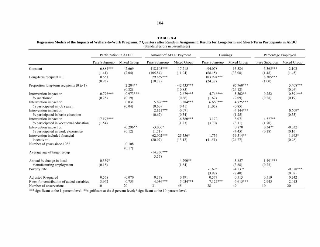
104

TABLE A.4

Regression Models of the Impacts of Welfare-to-Work Programs, 7 Quarters after Random Assignment: Results for Long-Term and Short-Term Participants in AFDC (Standard errors in parentheses)


Pure Subgroup Mixed Group Pure Subgroup Mixed Group Pure Subgroup Mixed Group Pure Subgroup Mixed Group

Constant 6.884*** -2.669 418.105*** 17.215 -94.078 15.584 5.365*** 2.103 (1.41) (2.04) (105.84) (11.04) (68.15) (33.08) (1.48) (1.45) Long-term recipient = 1 0.651 29.659*** 103.994*** 6.305*** (0.93) (10.77) (24.37) (1.00) Proportion long-term recipients (0 to 1) 2.204** -42.433*** 95.760*** 5.408*** (0.82) (10.85) (24.12) (0.96) Intervention impact on -0.798*** 0.973*** 2.679*** 4.746*** 5.562** 0.252 0.591***

% sanctioned (0.25) (0.19) (0.66) (1.62) (2.09) (0.28) (0.19) Intervention impact on 0.031 5.696*** 3.384*** 6.660*** 4.725***

% participated in job search (0.04) (0.60) (0.41) (1.03) (0.85) Intervention impact on 2.121*** -0.071 -4.144*** 0.609*

% participated in basic education (0.67) (0.54) (1.25) (0.35) Intervention impact on 17.198*** -6.580*** 3.172 3.071 4.527**

% participated in vocational education (1.54) (1.23) (3.70) (3.11) (1.70) Intervention impact on -0.296** -3.006* 0.870 0.347* -0.032

% participated in work experience (0.12) (1.71) (4.45) (0.18) (0.16) Intervention included financial -62.002*** -25.556* 1.736 -59.514** 1.993*

incentive=1 (20.07) (13.12) (41.51) (24.27) (0.98) Number of years since 1982 0.108 (0.17) Average age of target group -14.250*** 3.578 Annual % change in local -0.359* 4.290** 3.857 -1.491***

manufacturing employment (0.18) (1.84) (3.68) (0.23) Poverty rate -1.695 -4.537* -0.378*** (3.92) (2.40) (0.08) Adjusted R-squared 0.568 -0.070 0.378 0.391 0.577 0.513 0.519 0.242 F-test for contribution of added variables 3.962 0.753 4.036*** 5.034*** 7.127*** 6.615*** 2.945 2.013 Number of observations 10 20 31 45 28 49 10 20 ***significant at the 1-percent level; **significant at the 5-percent level; *significant at the 10-percent level.

105

FIGURE 1

HOW WELFARE POLICIES MIGHT AFFECT CHILDREN

Source: Welfare Reform and Children: A Synthesis of Impacts in Five States. 2005. Washington DC: Administration for Children and Families. Retrieved March 17, 2005, from http://www.acf.hhs.gov/programs/opre/welfare_employ/ch_outcomes/reports/welfare_reform_children/welfare_reform_toc.html.

107

Table 1 U.S. Welfare-to-Work Evaluations Included in the Database

Program Title

Short Program

Name Evaluator/Author

Midpoint of Random Assignment

FinancialIncentiveScheme

MANDATORY Greater Avenues for Independence Program GAIN

(California) MDRC 1989

Job Search and Work Experience in Cook County Cook County MDRC 1985 Community Work Experience Demonstrations West Virginia MDRC 1983 WORK Program Arkansas MDRC 1983 Employment Initiatives Baltimore MDRC 1983 Saturation Work Initiative Model SWIM

(San Diego) MDRC 1985

Employment Services Program Virginia MDRC 1984 Project Independence (Florida’s JOBS Program) Florida MDRC 1991 Jobs First Connecticut MDRC 1996 √ Family Transition Program FTP

(Florida) MDRC 1994

Los Angeles Jobs-First GAIN Evaluation Los Angeles MDRC 1996 San Diego Job Search and Work Experience Demonstration San Diego MDRC 1983 National Evaluation of Welfare-to-Work Strategies NEWWS MDRC 1993 Minnesota Family Investment Program MFIP MDRC 1994 √ Vermont’s Welfare Restructuring Project. Vermont MDRC 1995 √ Teenage Parent Demonstration Teenage

Parents Mathematica Policy

Research (MPR) 1988

Wisconsin Welfare Employment Experiment Wisconsin University of Wisconsin 1988 Ohio Transitions to Independence Demonstration Ohio Abt Associates 1990 Indiana Welfare Reform Program Indiana Abt Associates 1995 Saturation Work Program Philadelphia PA Department of Public

Welfare 1986

To Strengthen Michigan Families TSMF (Michigan)

Abt Associates 1993

A Better Chance ABC (Delaware)

Abt Associates 1996

Virginia Independence Program VIEW MPR 1996 Family Investment Program FIP(Iowa) MPR 1994 Personal Responsibility and Employment Program PREP

(Colorado) The Centers of the

University of Colorado 1995

Self-Sufficiency First/Pay for Performance Program SSF/PFP (Wisconsin)

Institute for Research on Poverty, University of

WI

1995

California Work Pays Demonstration Program (financial incentive only)

CWPDP UCLA School of Public Policy and Social Research

1993 √

Child Assistance Program CAP (New York)

Abt Associates 1989 √

VOLUNTARY Supported Work SW MDRC 1976 Homemaker Health Aide HHA Abt Associates 1984 Training Opportunities in the Private Sector Program TOPS

(Maine) MDRC 1984

New Jersey Grant Diversion Project NJGD MDRC 1985 New York State Comprehensive Employment Opportunities

Support Centers Program CEOSC Abt 1989

Self-Sufficiency Project SSP (Canada) MDRC 1994 √ Self-Sufficiency Project Plus SSP+ Canada) SRDC 1985 √

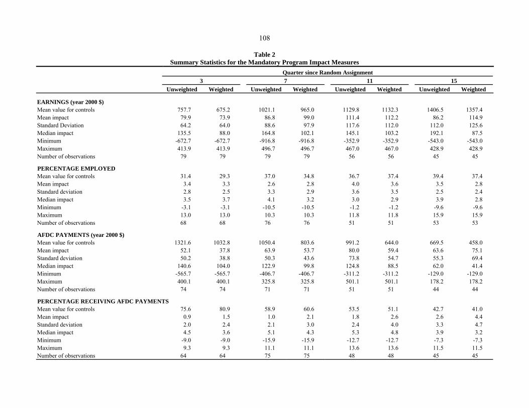
108

Table 2 Summary Statistics for the Mandatory Program Impact Measures

Quarter since Random Assignment 3 7 11 15 Unweighted Weighted Unweighted Weighted Unweighted Weighted Unweighted Weighted

EARNINGS (year 2000 $) Mean value for controls 757.7 675.2 1021.1 965.0 1129.8 1132.3 1406.5 1357.4 Mean impact 79.9 73.9 86.8 99.0 111.4 112.2 86.2 114.9 Standard Deviation 64.2 64.0 88.6 97.9 117.6 112.0 112.0 125.6 Median impact 135.5 88.0 164.8 102.1 145.1 103.2 192.1 87.5 Minimum -672.7 -672.7 -916.8 -916.8 -352.9 -352.9 -543.0 -543.0 Maximum 413.9 413.9 496.7 496.7 467.0 467.0 428.9 428.9 Number of observations 79 79 79 79 56 56 45 45

PERCENTAGE EMPLOYED Mean value for controls 31.4 29.3 37.0 34.8 36.7 37.4 39.4 37.4 Mean impact 3.4 3.3 2.6 2.8 4.0 3.6 3.5 2.8 Standard deviation 2.8 2.5 3.3 2.9 3.6 3.5 2.5 2.4 Median impact 3.5 3.7 4.1 3.2 3.0 2.9 3.9 2.8 Minimum -3.1 -3.1 -10.5 -10.5 -1.2 -1.2 -9.6 -9.6 Maximum 13.0 13.0 10.3 10.3 11.8 11.8 15.9 15.9 Number of observations 68 68 76 76 51 51 53 53

AFDC PAYMENTS (year 2000 $) Mean value for controls 1321.6 1032.8 1050.4 803.6 991.2 644.0 669.5 458.0 Mean impact 52.1 37.8 63.9 53.7 80.0 59.4 63.6 75.1 Standard deviation 50.2 38.8 50.3 43.6 73.8 54.7 55.3 69.4 Median impact 140.6 104.0 122.9 99.8 124.8 88.5 62.0 41.4 Minimum -565.7 -565.7 -406.7 -406.7 -311.2 -311.2 -129.0 -129.0 Maximum 400.1 400.1 325.8 325.8 501.1 501.1 178.2 178.2 Number of observations 74 74 71 71 51 51 44 44

PERCENTAGE RECEIVING AFDC PAYMENTS Mean value for controls 75.6 80.9 58.9 60.6 53.5 51.1 42.7 41.0 Mean impact 0.9 1.5 1.0 2.1 1.8 2.6 2.6 4.4 Standard deviation 2.0 2.4 2.1 3.0 2.4 4.0 3.3 4.7 Median impact 4.5 3.6 5.1 4.3 5.3 4.8 3.9 3.2 Minimum -9.0 -9.0 -15.9 -15.9 -12.7 -12.7 -7.3 -7.3 Maximum 9.3 9.3 11.1 11.1 13.6 13.6 11.5 11.5 Number of observations 64 64 75 75 48 48 45 45

109

Table 3 Means of Available Explanatory Variables

Number of

Observations Mean Standard Deviation

Characteristics of Interventions Program impacts on the percentage who:

Were sanctioned 62 6.37 7.77 Participated in job search 66 21.12 13.95 Participated in basic education 66 7.31 11.90 Participated in vocational education 66 2.81 5.02 Participated in work experience 76 2.86 5.57

Percentage of interventions that included financial incentives 79 31.65 46.81 Percentage of interventions that only provided financial incentives 79 15.19 36.12 Monthly amount of financial incentive after 13 months in a job in

year 2000 dollars 79 82.75 135.68 Percentage of interventions that included time limit 79 15.19 36.12 Percentage of interventions targeted at 2-parent families 79 20.25 40.45 Net cost to the government in year 2000 dollars 61 1,853.41 1,711.49 Number of years since 1982 to mid-point of random assignment 79 8.85 3.69

Characteristics of Target Population Average age of target group 71 31.02 3.92 Average number of children in family 62 1.94 0.33 Percentage of target population:

Employed during year before random assignment 63 48.33 17.41 On AFDC for at least 2 years before random assignment 63 46.08 23.92 With either a high school degree or a GED 62 51.50 11.08 Who were under 25 years of age 58 26.64 21.93 With at least one child under 6 years of age 51 50.71 23.56 Who were white 77 41.24 23.36 Who were black 76 36.02 25.96 Who were Hispanic 70 17.24 14.73

Socioeconomic Conditions at Site Maximum monthly AFDC payment for a family of 3 in year 2000

dollars 79 602.67 199.43 Median annual household income in year 2000 dollars 79 40,237.38 6,670.37 Poverty rate 79 14.61 4.96 Unemployment rate 79 6.36 2.34 Percentage of workforce in manufacturing employment 79 12.99 5.16 Annual percentage change in manufacturing employment 79 1.11 4.49 Percentage of sites that at first sanction specified minimum length

or terminated full family benefits 79 6.33 24.50

110

Table 4 Regression Models of the Impacts of Welfare-to-Work Programs on Earnings

(Standard errors in parentheses) Quarter since Random Assignment 3 7 11 15 Unweighted Weighted Unweighted Weighted Unweighted Weighted Unweighted Weighted Constant 11.644 -126.070 3.714 -5.523 -1.695 217.358 -62.258 -128.846 (30.80) (143.27) (41.62) (141.25) (47.61) (149.34) (78.61) (297.33) Intervention impact on 1.340 2.426* 4.586*** 6.337*** 2.217 -0.652 0.085 0.713

% sanctioned (1.17) (1.44) (1.43) (1.92) (1.53) (2.20) (2.01) (3.15) Intervention impact on 2.395*** 1.924** 2.280*** 1.711** 3.582*** 3.486*** 2.025 1.909

% participated in job search (0.77) (0.81) (0.80) (0.85) (0.97) (1.05) (1.42) (1.59) Intervention impact on -0.818 -1.859 -0.688 -1.873 0.967 1.373 -1.266 -1.795

% participated in basic education (1.09) (1.18) (1.11) (1.24) (1.13) (1.25) (1.90) (2.35) Intervention impact on -6.276** -4.889* -2.069 1.579 -6.791** -4.542 6.403 7.335

% participated in vocational education (2.58) (2.75) (2.63) (2.88) (3.09) (3.36) (4.88) (6.01) Intervention impact on 0.583 -1.238 0.919 -2.763 6.530* 6.487* 4.212 1.826

% participated in work experience (2.08) (2.25) (2.45) (2.74) (3.32) (3.74) (5.24) (7.06) Intervention included financial incentive=1 -63.761*** -46.481** -37.343* -44.170* -12.477 -20.880 27.623 16.641 (19.53) (21.31) (21.13) (23.06) (23.02) (25.70) (34.93) (39.02) Intervention included time limit=1 -3.916 -5.517 10.019 27.207 43.370 68.010** -5.058 5.527 (23.63) (25.47) (25.88) (31.26) (27.88) (32.95) (38.84) (46.82) Number of years since 1982 4.431 0.497 2.933 -1.452 2.845 5.583 10.209 8.677 (2.74) (3.40) (3.49) (4.22) (3.99) (5.15) (6.76) (8.15) Two-parent family target group=1 62.691* 40.910 35.280 38.581 -54.159 -3.799 38.792 18.250 (34.25) (40.40) (33.15) (39.22) (34.60) (40.94) (50.73) (72.87) Average age of target group 4.694 5.413 -2.256 4.455 (4.20) (4.04) (4.33) (7.42) % of target group with recent employment 0.425 -1.041 -3.147*** -0.424 (0.85) (0.87) (0.91) (1.53) Annual % change in local 7.636*** 7.693** -2.617 -2.444

manufacturing employment (2.82) (3.15) (3.36) (4.90) Poverty rate 0.943 -4.774** -1.087 -2.037 (2.19) (2.26) (2.72) (5.10) Adjusted R-squared 0.349 0.386 0.201 0.239 0.228 0.279 0.011 -0.075 F-test for regression 5.640*** 3.179*** 2.802*** 1.054 F-test for contribution of added variables 2.057* 1.855 1.825 0.299 Number of observations 79 79 79 79 56 56 45 45 ***significant at the 1-percent level; **significant at the 5-percent level; *significant at the 10-percent level

111

Table 5 Regression Models of the Impacts of Welfare-to-Work Programs on Percentage Employed

(Standard errors in parentheses) Quarter since Random Assignment 3 7 11 15 Unweighted Weighted Unweighted Weighted Unweighted Weighted Unweighted Weighted Constant -2.059** -3.983 -1.519 -5.193* -0.761 9.641** -3.330 -1.868 (0.79) (2.74) (0.92) (3.08) (1.43) (3.78) (2.09) (5.03) Intervention impact on 0.009 0.060* 0.106*** 0.180*** 0.029 -0.083 -0.036 -0.030

% sanctioned (0.03) (0.03) (0.03) (0.04) (0.03) (0.05) (0.04) (0.06) Intervention impact on 0.129*** 0.098*** 0.084*** 0.068*** 0.124*** 0.134*** 0.148*** 0.142***

% participated in job search (0.02) (0.02) (0.02) (0.02) (0.03) (0.03) (0.04) (0.04) Intervention impact on 0.013 -0.040 0.035 -0.014 0.043 0.047 0.069** 0.048

% participated in basic education (0.02) (0.03) (0.02) (0.03) (0.03) (0.03) (0.03) (0.04) Intervention impact on -0.372*** -0.314*** -0.162** -0.047 -0.202** -0.125 -0.004 0.006

% participated in vocational education (0.06) (0.07) (0.06) (0.07) (0.08) (0.08) (0.12) (0.13) Intervention impact on 0.071* 0.025 0.074* -0.037 0.087 0.091 -0.155 -0.201

% participated in work experience (0.04) (0.04) (0.04) (0.05) (0.07) (0.08) (0.11) (0.12) Intervention included financial incentive=1 -1.189** -0.741 -0.198 -0.097 -0.204 -0.786 -0.791 -0.718 (0.48) (0.51) (0.52) (0.56) (0.63) (0.67) (0.87) (0.82) Intervention included time limit=1 0.038 -0.303 1.060 1.368 3.301*** 3.283*** 3.791*** 3.788*** (0.66) (0.70) (0.74) (0.83) (0.83) (0.93) (0.99) (1.12) Number of years since 1982 0.406*** 0.206** 0.204*** 0.051 0.120 0.228 0.304* 0.276 (0.07) (0.09) (0.08) (0.10) (0.11) (0.14) (0.16) (0.18) Two-parent family target group=1 -0.966 -1.696** -1.782*** -2.146*** 0.457 2.197** 0.113 0.783 (0.63) (0.76) (0.65) (0.80) (0.73) (0.86) (0.92) (1.03) Average age of target group 0.146* 0.247*** -0.154 0.069 (0.08) (0.09) (0.10) (0.12) % of target group with recent employment 0.013 -0.014 -0.101*** -0.037 (0.02) (0.02) (0.02) (0.03) Annual % change in local 0.270*** 0.129* -0.093 -0.060

manufacturing employment (0.06) (0.07) (0.07) (0.08) Poverty rate -0.046 -0.129** -0.097 -0.092 (0.05) (0.05) (0.06) (0.08) Adjusted R-squared 0.355 0.403 0.191 0.221 0.328 0.493 0.261 0.279 F-test for regression 5.102*** 2.967*** 3.715*** 3.037*** F-test for contribution of added variables 2.158* 1.636 4.330*** 1.274 Number of observations 68 68 76 76 51 51 53 53 ***significant at the 1-percent level; **significant at the 5-percent level; *significant at the 10-percent level.

112

Table 6 Regression Models of the Impacts of Welfare-to-Work Programs on Amount of AFDC Payment

(Standard errors in parentheses) Quarter Since Random Assignment 3 7 11 15 Unweighted Weighted Unweighted Weighted Unweighted Weighted Unweighted Weighted Constant 29.429* 119.895** -20.133 -177.367*** -174.792*** -203.292*** -36.465 -33.129 (16.66) (59.75) (18.87) (58.87) (26.77) (65.24) (28.12) (100.44) Intervention impact on 4.111*** 3.261*** 3.692*** 5.842*** 0.916* 3.290*** -0.125 0.672

% sanctioned (0.56) (0.66) (0.58) (0.83) (0.53) (1.01) (0.84) (1.17) Intervention impact on 1.406*** 0.973** 2.701*** 1.093*** 4.183*** 1.945*** 2.928*** 1.437*

% participated in job search (0.33) (0.37) (0.34) (0.39) (0.40) (0.51) (0.60) (0.85) Intervention impact on 1.673*** 1.143* 2.069*** -0.947 3.151*** -0.557 1.700** 1.251

% participated in basic education (0.51) (0.60) (0.51) (0.64) (0.54) (0.74) (0.68) (0.90) Intervention impact on -3.393*** 0.125 -1.988* 4.303*** -1.694 4.369*** -1.295 -1.376

% participated in vocational education (1.08) (1.28) (1.05) (1.28) (1.19) (1.46) (1.90) (2.36) Intervention impact on -1.640 -0.840 -1.294 -4.835*** 1.865 -1.958 -1.897 -1.278

% participated in work experience (1.11) (1.22) (1.04) (1.30) (1.28) (1.61) (2.18) (2.97) Intervention included financial incentive=1 -118.585*** -138.649*** -84.248*** -111.666*** -78.413*** -107.303*** -20.716 -26.539 (8.82) (9.87) (8.38) (9.80) (9.93) (11.98) (16.43) (19.77) Intervention included time limit=1 18.760* 31.165*** 32.241*** 64.701*** 43.899*** 73.533*** 38.507** 55.726*** (10.43) (11.19) (11.23) (13.10) (11.36) (13.68) (15.69) (18.70) Number of years since 1982 -1.840 -0.250 0.558 -4.144* 13.353*** 5.778** 5.826** 2.687 (1.42) (1.62) (1.62) (2.17) (2.02) (2.86) (2.32) (2.74) Two-parent family target group=1 61.322** 74.592*** 46.902** 4.649 7.911 -16.586 -97.158*** -81.327** (24.21) (25.51) (20.56) (23.10) (23.12) (25.18) (33.06) (38.10) Average age of target group -3.213 5.065*** 1.958 0.998 (2.00) (1.82) (1.82) (2.93) % of target group with recent employment -1.354*** -0.483 -1.009** -0.709 (0.31) (0.36) (0.39) (0.62) Annual % change in local -0.572 6.925*** 5.122*** 4.672**

manufacturing employment (1.21) (1.54) (1.50) (1.88) Maximum AFDC payment for a family of 3 0.116*** 0.175*** 0.247*** 0.085 (0.03) (0.03) (0.04) (0.06) Adjusted R-squared 0.376 0.376 0.329 0.407 0.387 0.472 0.473 0.589 F-test for regression 5.880*** 4.819*** 4.508*** 5.283*** F-test for contribution of added variables 1.017 2.994** 2.650** 3.416** Number of observations 74 74 71 71 51 51 44 44 ***significant at the 1-percent level; **significant at the 5-percent level; *significant at the 10-percent level.

113

Table 7 Regression Models of the Impacts of Welfare-to-Work Programs on Percentage Participating in AFDC

(Standard errors in parentheses) Quarter Since Random Assignment 3 7 11 15 Unweighted Weighted Unweighted Weighted Unweighted Weighted Unweighted Weighted Constant 3.877*** 5.159** 2.810*** -1.755 1.846 4.321 -1.825 0.360 (0.75) (2.33) (0.85) (3.08) (1.32) (4.07) (1.65) (5.78) Intervention impact on 0.075*** 0.072** 0.117*** 0.181*** 0.103*** 0.107* 0.060 0.071

% sanctioned (0.02) (0.03) (0.03) (0.05) (0.04) (0.06) (0.05) (0.08) Intervention impact on 0.003 -0.001 0.057*** 0.026 0.085*** 0.053* 0.054 0.066*

% participated in job search (0.02) (0.02) (0.02) (0.02) (0.02) (0.03) (0.03) (0.04) Intervention impact on -0.021 -0.011 -0.019 -0.095*** -0.008 -0.055 0.063* 0.056

% participated in basic education (0.02) (0.02) (0.02) (0.03) (0.03) (0.03) (0.04) (0.05) Intervention impact on -0.085 -0.125** 0.002 0.131* -0.155** -0.078 -0.194* -0.229*

% participated in vocational education (0.05) (0.06) (0.06) (0.07) (0.08) (0.08) (0.10) (0.13) Intervention impact on -0.074* -0.056 -0.074 -0.157*** 0.031 -0.042 0.136 0.074

% participated in work experience (0.04) (0.05) (0.05) (0.06) (0.08) (0.09) (0.11) (0.16) Intervention included financial incentive=1 -6.006*** -6.262*** -5.424*** -5.52***7 -5.703*** -5.963*** -0.452 -0.197 (0.46) (0.50) (0.55) (0.63) (0.70) (0.82) (0.84) (1.10) Intervention included time limit=1 1.121* 0.835 2.043*** 3.301*** 4.659*** 6.194*** 1.884* 2.974** (0.62) (0.64) (0.74) (0.81) (0.84) (0.93) (0.99) (1.42) Number of years since 1982 -0.109* -0.112 -0.110 -0.249** -0.032 -0.196 0.438*** 0.328* (0.06) (0.08) (0.07) (0.10) (0.11) (0.15) (0.14) (0.18) Two-parent family target group=1 -1.664*** -1.783** -2.660*** -3.722*** -5.044*** -4.601*** -4.843*** -3.638** (0.56) (0.69) (0.68) (0.88) (0.82) (1.04) (1.17) (1.70) Average age of target group -0.052 0.159 0.025 0.057 (0.07) (0.10) (0.11) (0.16) % of target group with recent employment 0.021 -0.021 -0.07***0 -0.045 (0.01) (0.02) (0.02) (0.04) Annual % change in local 0.050 0.202*** 0.190** 0.006

manufacturing employment (0.06) (0.07) (0.09) (0.10) Maximum AFDC payment for a family of 3 -0.001 0.004** 0.004* -0.002 (0.00) (0.00) (0.00) (0.00) Adjusted R-squared 0.444 0.418 0.425 0.447 0.469 0.494 0.456 0.456 F-test for regression 6.593*** 7.086*** 5.605*** 5.095*** F-test for contribution of added variables 0.388 1.626 1.475 1.009 Number of observations 64 64 75 75 48 48 45 45 ***significant at the 1-percent level; **significant at the 5-percent level; *significant at the 10-percent level.

114

Table 8 Sensitivity Tests of Regression Models of the Impacts on Earnings (7th Quarter)

(Standard errors in parentheses) [1] [2] [3] [4] [5] Constant -5.523 180.587 -54.502 92.961 -2.906 (141.25) (167.48) (141.93) (188.81) (149.25) Intervention impact on 6.337*** 6.170*** 6.608*** 3.328 6.773***

% sanctioned (1.92) (2.29) (1.94) (2.85) (2.13) Intervention impact on 1.711** 1.510 1.610* 3.141** 1.701*

% participated in job search (0.85) (1.01) (0.85) (1.23) (0.92) Intervention impact on -1.873 -0.686 -2.221* 0.053 -1.997

% participated in basic education (1.24) (1.47) (1.25) (1.68) (1.33) Intervention impact on 1.579 -0.370 0.937 -0.924 1.906

% participated in vocational education (2.88) (3.42) (2.89) (3.46) (3.09) Intervention impact on -2.763 -3.945 -2.965 0.118 -3.153

% participated in work experience (2.74) (3.25) (2.75) (3.79) (2.89) Intervention included financial incentive=1 -44.170* -29.174 -45.387* -147.741** -38.148 (23.06) (27.31) (23.14) (64.80) (24.09) Intervention included time limit=1 27.207 -10.960 27.091 109.571 32.577 (31.26) (36.96) (31.32) (66.05) (33.49) Number of years since 1982 -1.452 6.167 -2.703 9.926 -3.297 (4.22) (5.02) (4.25) (6.97) (4.42) Two-parent family target group=1 38.581 19.958 -3.928 6.894 36.847 (39.22) (48.52) (41.12) (64.82) (40.66) Average age of target group 5.413 1.674 6.990* -0.260 6.219 (4.04) (4.80) (4.07) (5.45) (4.29) % of target group with recent employment -1.041 -2.320** -0.705 -1.258 -1.101 (0.87) (1.03) (0.87) (1.16) (0.91) Annual % change in local 7.693** 7.185* 7.382** 5.514 8.265**

manufacturing employment (3.15) (3.76) (3.19) (4.74) (3.32) Poverty rate -4.774** -9.846*** -4.486* -6.291* -5.310** (2.26) (2.67) (2.26) (3.71) (2.35) Adjusted R-squared 0.239 0.089 0.287 0.381 0.238 Number of observations 79 79 75 53 79 ***significant at the 1-percent level; **significant at the 5-percent level; *significant at the 10-percent level. Legend: [1] Original estimates, [2] Unweighted estimates, [3] Observations with two highest and lowest impacts omitted, [4] Observations with missing data omitted, [5] Observation using same controls given half weight.

115

Table 9 Sensitivity Tests of Regression Models of the Impacts on Percentage Employed (7th Quarter)


[1] [2] [3] [4] [5] Constant -5.193* -1.326 -3.748 -4.578 -5.470 (3.08) (7.37) (3.11) (3.63) (3.32) Intervention impact on 0.180*** 0.207** 0.159*** 0.111** 0.217***

% sanctioned (0.04) (0.10) (0.04) (0.05) (0.05) Intervention impact on 0.068*** 0.064 0.059*** 0.100*** 0.072***

% participated in job search (0.02) (0.04) (0.02) (0.02) (0.02) Intervention impact on -0.014 0.021 -0.024 0.028 -0.034

% participated in basic education (0.03) (0.06) (0.03) (0.03) (0.03) Intervention impact on -0.047 -0.099 -0.011 -0.117 -0.008

% participated in vocational education (0.07) (0.16) (0.07) (0.08) (0.08) Intervention impact on -0.037 -0.002 -0.009 0.048 -0.077

% participated in work experience (0.05) (0.12) (0.05) (0.06) (0.06) Intervention included financial incentive=1 -0.097 -0.083 -0.132 0.972 -0.099 (0.56) (1.41) (0.56) (1.30) (0.59) Intervention included time limit=1 1.368 2.321 0.824 1.861 1.894** (0.83) (1.56) (0.84) (1.41) (0.90) Number of years since 1982 0.051 0.011 0.113 0.262** -0.055 (0.10) (0.20) (0.10) (0.13) (0.11) Two-parent family target group=1 -2.146*** -1.451 -1.588* -1.614 -1.728** (0.80) (1.45) (0.81) (1.07) (0.82) Average age of target group 0.247*** 0.163 0.197** 0.105 0.290*** (0.09) (0.21) (0.09) (0.10) (0.10) % of target group with recent employment -0.014 -0.047 -0.022 -0.012 -0.016 (0.02) (0.04) (0.02) (0.02) (0.02) Annual % change in local 0.129* 0.181 0.096 -0.021 0.180**

manufacturing employment (0.07) (0.14) (0.07) (0.09) (0.08) Poverty rate -0.129** -0.129 -0.125** -0.033 -0.145*** (0.05) (0.10) (0.05) (0.08) (0.05) Adjusted R-squared 0.221 0.107 0.208 0.260 0.290 Number of observations 76 76 72 56 76 ***significant at the 1-percent level; **significant at the 5-percent level; *significant at the 10-percent level. Legend: [1] Original estimates, [2] Unweighted estimates, [3] Observations with two highest and lowest impacts omitted, [4] Observations with missing data omitted, [5] Observation using same controls given half weight.

116

Table 10 Sensitivity Tests of Regression Models of the Impacts on Amount of AFDC Payments

(7th Quarter) (Standard errors in parentheses)

[1] [2] [3] [4] [5] Constant -177.367*** -94.451 -22.656 89.217 -126.368** (58.87) (206.03) (58.96) (68.64) (62.27) Intervention impact on 5.842*** 4.724 2.961*** 0.887 6.208***

% sanctioned (0.83) (2.89) (0.87) (1.11) (0.94) Intervention impact on 1.093*** 3.021** 1.801*** 1.835*** 1.690***

% participated in job search (0.39) (1.33) (0.37) (0.45) (0.40) Intervention impact on -0.947 1.718 1.317** 1.497** -0.024

% participated in basic education (0.64) (1.55) (0.61) (0.69) (0.67) Intervention impact on 4.303*** 0.166 -1.385 -2.129 1.766

% participated in vocational education (1.28) (3.73) (1.26) (1.34) (1.33) Intervention impact on -4.835*** -0.749 -2.033 -1.591 -5.838***

% participated in work experience (1.30) (3.23) (1.33) (1.47) (1.40) Intervention included financial incentive=1 -111.666*** -54.605 -82.015*** -353.025*** -76.981*** (9.80) (41.12) (9.37) (23.44) (9.50) Intervention included time limit=1 64.701*** 25.285 31.286** 261.099*** 48.564*** (13.10) (53.23) (14.18) (23.78) (14.88) Number of years since 1982 -4.144* 3.687 -1.185 5.419* -7.036*** (2.17) (5.86) (2.16) (2.75) (2.29) Two-parent family target group=1 4.649 58.552 28.321 40.532 37.972 (23.10) (43.11) (23.41) (31.99) (24.98) Average age of target group 5.065*** 1.519 3.943** 1.803 8.166*** (1.82) (5.71) (1.81) (2.07) (1.91) % of target group with recent employment -0.483 -0.796 -0.769** -0.911** -0.503 (0.36) (1.16) (0.38) (0.43) (0.40) Annual % change in local 6.925*** 2.225 5.124*** 3.349* 7.261***

manufacturing employment (1.54) (3.60) (1.54) (1.84) (1.63) Maximum AFDC payment for a family of 3 0.175*** 0.092 -2.420** -6.988*** -2.353** (0.03) (3.31) (1.02) (1.28) (1.08) Adjusted R-squared 0.407 0.160 0.405 0.733 0.324 Number of observations 71 71 67 56 71 ***significant at the 1-percent level; **significant at the 5-percent level; *significant at the 10-percent level. Legend: [1] Original estimates, [2] Unweighted estimates, [3] Observations with two highest and lowest impacts omitted, [4] Observations with missing data omitted, [5] Observation using same controls given half weight.

117

Table 11 Sensitivity Tests of Regression Models of the Impacts on Percentage Participating in AFDC

(7th Quarter) (Standard errors in parentheses)

[1] [2] [3] [4] [5] Constant -1.755 -1.961 -1.259 5.095 -2.564 (3.08) (8.31) (3.36) (3.59) (2.76) Intervention impact on 0.181*** 0.141 0.173*** 0.014 0.190***

% sanctioned (0.05) (0.11) (0.05) (0.05) (0.04) Intervention impact on 0.026 0.053 0.031 0.016 0.042**

% participated in job search (0.02) (0.05) (0.02) (0.02) (0.02) Intervention impact on -0.095*** -0.057 -0.058** -0.019 -0.076***

% participated in basic education (0.03) (0.07) (0.03) (0.03) (0.02) Intervention impact on 0.131* -0.021 0.067 -0.048 0.077

% participated in vocational education (0.07) (0.17) (0.07) (0.08) (0.06) Intervention impact on -0.157*** -0.091 -0.180*** 0.050 -0.183***

% participated in work experience (0.06) (0.13) (0.06) (0.07) (0.05) Intervention included financial incentive=1 -5.527*** -4.970*** -4.114*** -14.738*** -4.406*** (0.63) (1.67) (0.65) (1.28) (0.54) Intervention included time limit=1 3.301*** 3.879** 3.157*** 11.922*** 3.034*** (0.81) (1.75) (0.85) (1.38) (0.71) Number of years since 1982 -0.249** -0.165 -0.296*** 0.262** -0.331*** (0.10) (0.21) (0.10) (0.13) (0.09) Two-parent family target group=1 -3.722*** -4.133** -2.269** -1.338 -3.748*** (0.88) (1.76) (0.99) (0.98) (0.75) Average age of target group 0.159 0.145 0.218** -0.009 0.265*** (0.10) (0.23) (0.10) (0.10) (0.08) % of target group with recent employment -0.021 0.007 -0.022 -0.008 -0.009 (0.02) (0.05) (0.02) (0.02) (0.02) Annual % change in local 0.202*** 0.030 0.176** -0.030 0.196***

manufacturing employment (0.07) (0.15) (0.07) (0.09) (0.06) Maximum AFDC payment for a family of 3 0.004** 0.049 -0.008 -0.200** -0.034 (0.00) (0.12) (0.06) (0.08) (0.05) Adjusted R-squared 0.447 0.311 0.398 0.691 0.382 Number of observations 75 75 70 57 75 ***significant at the 1-percent level; **significant at the 5-percent level; *significant at the 10-percent level. Legend: [1] Original estimates, [2] Unweighted estimates, [3] Observations with two highest and lowest impacts omitted, [4] Observations with missing data omitted, [5] Observation using same controls given half weight.

118

Table 12 Comparison of Estimated Impacts and Regression-Predicted Impacts for the 7th Quarter

Randomly Selected Interventions

Earnings % Employed Average AFDC Payments % Receiving AFDC

Case Estimated

Impact Predicted Impact

Absolute Difference

Estimated Impact

Predicted Impact

Absolute Difference

Estimated Impact

Predicted Impact

Absolute Difference

Estimated Impact

Predicted Impact

Absolute Difference

1 2.57 89.06 86.49 2.08 1.79 0.29 14.23 -97.99 112.22 5.30 -3.99 9.29 2 404.90 142.21 262.69 3.80 6.35 2.55 -44.56 29.56 74.11 -0.20 0.92 1.12 3 -77.51 80.28 157.78 -2.70 1.18 3.88 9.01 253.61 244.60 5.40 -1.23 6.63 4 -3.96 36.27 40.23 -0.40 2.95 3.35 275.14 -26.28 301.42 0.50 3.59 3.09 5 211.26 214.00 2.74 5.30 0.69 4.61 9.97 38.75 28.78 -1.50 2.35 3.85 6 -53.38 -40.80 12.58 -4.80 -2.27 2.53 62.71 16.85 45.86 3.40 4.31 0.91 7 90.04 172.68 82.64 2.80 3.24 0.44 -2.79 178.27 181.06 -4.30 -2.65 1.65 8 150.08 -42.37 192.46 4.80 2.85 1.95 175.25 100.52 74.74 2.40 4.50 2.10 9 31.50 -24.68 56.18 1.00 2.74 1.74 108.99 86.39 22.60 5.30 3.56 1.74 10 -96.74 0.61 97.35 10.20 4.24 5.96 129.45 199.10 69.65 3.80 4.45 0.65 Average 65.88 62.72 99.11 2.21 2.37 2.73 73.74 77.88 115.50 2.01 1.58 3.10 Most Recent Interventions

Earnings % Employed Average AFDC Payments % Receiving AFDC

Case Estimated Impact

Predicted Impact

Absolute Difference

Estimated Impact

Predicted Impact

Absolute Difference

Estimated Impact

Predicted Impact

Absolute Difference

Estimated Impact

Predicted Impact

Absolute Difference

A 93.17 109.41 16.24 8.10 3.95 4.15 64.90 -20.49 85.40 5.40 -2.21 7.61 B 255.43 62.87 192.56 7.60 3.72 3.88 49.20 6.57 42.63 5.70 -1.40 7.10 C 211.26 248.60 37.35 6.30 6.53 0.23 129.45 200.13 70.69 4.70 5.84 1.14 D 277.54 321.02 43.48 7.20 3.38 3.82 181.23 188.14 6.91 4.60 2.98 1.62 E -18.91 152.01 170.92 -0.10 5.31 5.41 50.83 62.92 12.09 0.80 2.64 1.84 Average 163.70 178.78 92.11 5.82 4.58 3.50 95.12 87.45 43.54 4.24 1.57 3.86

119

Table 13 The Impact of Welfare-to-Work over Time

Control Variables Earnings % Employed AFDC Payments % Receiving AFDC Excluded Included Excluded Included Excluded Included Excluded Included Constant 16.189*** -106.468*** 1.895*** -3.362*** -11.119*** -155.903*** -0.460*** -1.261* (5.69) (33.37) (0.15) (0.86) (2.82) (14.14) (0.11) (0.74) Number of quarters 16.706*** 18.207*** 0.379*** 0.323*** 12.364*** 13.124*** 0.471*** 0.564*** (1.43) (1.37) (0.04) (0.04) (0.65) (0.65) (0.03) (0.03) Number of quarters squared -0.679*** -0.766*** -0.021*** -0.019*** -0.473*** -0.614*** -0.014*** -0.021*** (0.07) (0.07) (0.00) (0.00) (0.03) (0.03) (0.00) (0.00) Adjusted R-squared 0.078 0.361 0.043 0.369 0.048 0.484 0.112 0.464 Number of observations 857 857 875 875 857 857 906 906 Quarter of peak growth 12.3 11.9 8.9 8.4 13.1 10.7 17.1 13.6 Quarter at which zero impact reached 25.5 24.4 21.9 21.9 25.2 21.2 33.1 26.2 ***significant at the 1-percent level; **significant at the 5-percent level; *significant at the 10-percent level.

120

Table 14 Number of Quarterly Impact Estimates That Are Outliers, Quarters 3, 7, 11 and 15

Type of Outliers

Total

Not Outliers Outliers

Only Type A

Only Type B

Both Types A & B

Earnings 259 188 71 23 14 34 Percentage employed 248 123 125 53 25 47 Mean AFDC payment 240 153 87 37 19 31 Percentage receiving

AFDC 232 115 117 44 26 47

Legend: → Type A = Outlier before controlling for explanatory variables. Type B = Outlier after controlling for explanatory variables.

121

Table 15 Multiple Outlier Interventions, Quarters 3, 7, 11, and 15

Interventions with Multiple Outliers

Number of Interventions with at Least Two Outliers

Number of Outliers Accounted for by

Interventions with at Least Two Outliers

All

Interventions Any Type Type Ba Any Type Type Ba

Earnings 99 17 9 42 23 Percentage employed 87 42 21 99 46 Mean AFDC payment 90 27 15 69 35 Percentage receiving

AFDC 84 32 20 83 46 aIncludes some cases that are also outliers under Type A. Legend: → Type A = Outlier before controlling for explanatory variables. Type B = Outlier after controlling for explanatory variables. .

122

TABLE 16 Welfare-To-Work Interventions with Multiple Positive Outliers, by Type and Impact

Earnings % Employed AFDC Payments % Receiving AFDC Program Title

Site/Intervention Type A Type B Type A Type B Type A Type B Type A Type B

One-Parent Family Programs Greater Avenues for Independence Program Butte (1) 2 Riverside 3 3 4 3 4 (1) 2 WORK Program (Arkansas) Jefferson & Pulaski S 2 3 (1) Employment Initiatives (Baltimore) 3 Saturation Work Initiative Model (San Diego) 3 2 2 Jobs First (Connecticut) Manchester 2 2 (1) New Haven 2 (1) 2 (1) Family Transition Program (Florida) 2 2 (1) Los Angeles Jobs-First GAIN Evaluation 2 3 San Diego Job Search and Work Experience Demonstration Job search & work experience 2 (1) National Evaluation of Welfare-to-Work Strategies (NEWWS) Grand Rapids -LFA 2 (1) 2 2 3 2 Riverside-LFA 2 (1) 3 (1) 3 Riverside: HCD 2 3 Portland (OR) 3 (1) 3 2 3 4 3 Columbus-Integrated case mgt 4 (1) Minnesota Family Investment Program Urban—services & incentives 2 (1) Vermont Welfare Restructuring Project Rutland—services & incentives 2 2 California Work Pays Demonstration Alameda (1) 2 San Bernardino (1) 2 New York State Child Assistance Program Monroe (1) 3 3 Niagara (1) 2 2 Suffolk 2 Two-Parent Family Programs Greater Avenues for Independence Program Butte 3 3 2 (1) 2 2 Los Angeles 4 4 Riverside (1) 2 2 (1) San Diego 2 Saturation Work Initiative Model (San Diego) 3 (1) Los Angeles Jobs-First GAIN Evaluation 3 3 3 San Diego Job Search and Work Experience Demonstration Job search only 2 (1) Vermont Welfare Restructuring Project Combined areas—incentives only 2 2 California Work Pays Demonstration Alameda 3 3 San Bernardino 3 3 2 2 2 2 Legend: → Type A = Outlier before controlling for explanatory variables. Type B = Outlier after controlling for explanatory variables. LFA - Labor Force Attachment. HCD - Human Capital Development. Note: Positive outliers are defined as one standard deviation or more above the mean impacts in quarters 3, 7, 11, and 15.

123

Table 17 Welfare-to-Work Interventions with Multiple Negative Outliers, by Type and Impact

Earnings % Employed AFDC Payment % Receiving AFDC Program Title

Site/Intervention Type A Type B Type A Type B Type A Type B Type A Type B

One-Parent Family Programs Greater Avenues for Independence Program (GAIN) Butte (1) 2 Tulare 2 (1) 2 Employment Services Program (Virginia) 2 2 2 San Diego Job Search and Work Experience Demonstration Job search only 2 Project Independence (Florida) Duval 2 (1) National Evaluation of Welfare-to-Work Strategies (NEWWS) Detroit 2 Oklahoma City 4 Minnesota Family Investment Program (MFIP) Urban - service & incentives 3 3 3 3 Urban - incentives only 2 3 3 3 3 Rural - services & incentives 2 2 2 2 Vermont Welfare Restructuring Project Barre—Incentives only 2 2 Burlington - incentives only 2 (1) Newport - services & incentives (1) 2 Newport—Incentives only 2 2 Teenage Parent Demonstration Newark 2 Indiana Welfare Reform Program Cohort—1998-99 2 California Work Pays Demonstration Los Angeles 2 (1) 2 (1) New York State Child Assistance Program Niagara 2 (1) Two-Parent Family Programs Greater Avenues for Independence Program (GAIN) Alameda (1) 2 2 2 San Diego 2 (1) Tulare 1 2 3 2 (1) Employment Initiatives (Baltimore) 2 2 2 2 2 The San Diego Job Search and Work Experience Demonstration Job search & work experience (1) 2 Job search only 2 2 Minnesota Family Investment Program (MFIP) Urban—services & incentives 2 2 Urban + rural—services & incentives 3 (1) 3 3 Vermont Welfare Restructuring Project Combined areas—services & incentives 2 2 2 4 2 Combined areas—incentives only 3 2 3 2 4 1 Legend: → Type A = Outlier before controlling for explanatory variables. Type B = Outlier after controlling for explanatory variables. LFA - Labor Force Attachment. HCD - Human Capital Development. Note: Negative outliers are defined as one standard deviation or more below the mean impacts in quarters 3, 7, 11 and 15.

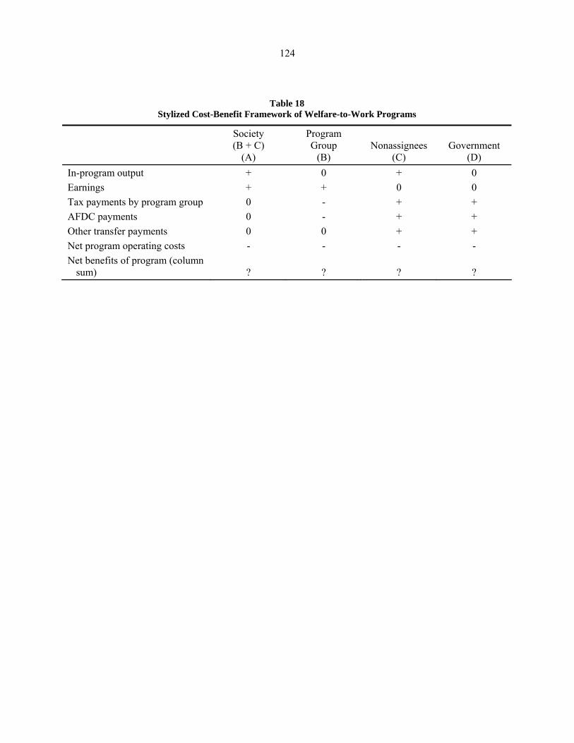
124

Table 18 Stylized Cost-Benefit Framework of Welfare-to-Work Programs

Society (B + C)

(A)

Program Group

(B) Nonassignees

(C) Government

(D) In-program output + 0 + 0 Earnings + + 0 0 Tax payments by program group 0 - + + AFDC payments 0 - + + Other transfer payments 0 0 + + Net program operating costs - - - - Net benefits of program (column

sum) ? ? ? ?

125

Table 19

Net Benefit-Costs of Interventions over Observation Period (year 2000 dollars)

Mean Standard Deviation Median

Unweighted Weighted Unweighted Weighted Unweighted Weighted Minimum Maximum No. of Obs.

Perspective

Program group $121 $122 $3,002 $2,932 $-54 $56 $-6,559 $11,040 49

Government -236 54 3088 2950 246 436 -9207 5287 49

Nonassignees -188 88 3133 2992 436 570 -9372 5287 49

Society 76 355 2928 2785 438 507 -5904 5966 49

Net cost to government 1,967 1,773 1,861 1,738 1,346 1,346 -290 8,613 49 Note: The observation period varied between evaluations, typically covering several years and, most frequently, five years.

126

Table 20 Regression Models of the Impacts of the Benefit-Cost Outcomes from Alternative Perspectives

(Standard errors in parentheses) Perspective Program Group Government Nonassignees Society

Constant -964.33 -10487.83 1957.22 4672.17 2130.83 4628.66 1513.32 -5620.21 (1658.9) (6826.2) (1719.0) (6664.3) (1713.6) (6711.4) (1627.5) (6023.3) Intervention impact on -99.42 -48.45 20.84 64.83 4.74 50.07 -28.22 67.47

% sanctioned (75.0) (85.4) (77.7) (83.4) (77.5) (83.9) (73.6) (75.3) Intervention impact on 31.99 26.28 -1.21 -44.04 -8.73 -50.11 7.71 -35.98

% participated in job search (31.3) (34.7) (32.4) (33.9) (32.3) (34.1) (30.7) (30.6) Intervention impact on 53.82 46.87 -104.85** -177.54**** -106.96** -175.82*** -39.22 -105.54**

% participated in basic education (44.6) (57.8) (46.2) (56.4) (46.1) (56.8) (43.8) (51.0) Intervention impact on -217.98* -282.42* -91.74 29.59 -106.44 9.77 -352.74*** -323.63**

% participated in vocational education (123.0) (139.4) (127.5) (136.1) (127.1) (137.0) (120.7) (123.0) Intervention impact on 70.13 29.83 -38.91 -4.73 5.03 40.53 84.08 78.98

% participated in work experience (89.4) (94.7) (92.6) (92.4) (92.4) (93.1) (87.7) (83.5) Intervention included financial 3735.60*** 4620.01*** -3686.69*** -5462.32*** -3830.52*** -5560.00*** -88.86 -766.41

incentive=1 (1103.3) (1263.2) (1143.3) (1233.3) (1139.7) (1242.0) (1082.4) (1114.7) Intervention included time limit=1 1612.98 1068.73 727.29 602.75 563.18 434.46 1956.49 1188.55 (1326.6) (1371.1) (1374.7) (1338.6) (1370.4) (1348.0) (1301.5) (1209.8) Number of years since 1982 32.67 -116.14 -51.00 -53.02 -46.66 -41.14 -48.66 -196.12 (156.4) (174.5) (162.1) (170.4) (161.6) (171.6) (153.4) (154.0) Two-parent family target group=1 -1541.57 -3159.42** 135.70 -1000.40 232.61 -892.60 -1566.91 -4331.89*** (1143.9) (1501.5) (1185.3) (1465.9) (1181.6) (1476.2) (1122.2) (1324.9) Average age of target group 334.09 -219.28 -215.89 130.52 (216.5) (211.4) (212.9) (191.1) % of target group with recent 67.84* 7.93 9.43 83.12**

employment (36.8) (35.9) (36.1) (32.4) Annual % change in local 90.88 77.92 53.26 142.51

manufacturing employment (153.2) (149.5) (150.6) (135.2) Maximum AFDC payment for a -4.2 8.0** 7.9** 2.7

family of 3 (3.2) (3.2) (3.2) (2.9) Adjusted R-squared 0.256 0.280 0.210 0.322 0.238 0.332 0.206 0.378 F-test for contribution of added variables 2.834** 1.324 2.422** 2.599* 2.662** 2.370* 2.385** 3.703 Number of observations 49 49 49 49 49 49 49 49 ***significant at the 1-percent level; **significant at the 5-percent level; *significant at the 10-percent level.

127

Table 21 Welfare-to-Work Evaluations Reporting Subgroup Impacts and Included in the Database

Program Title County AFDC

Applicants AFDC

Recipients

Employed in Year Before

RA

Not Employed in Year

Before RA

With High School

Diplomas

Without High School

Diplomas

Long-Term AFDC

Participants

Short-Term AFDC

Participants GAIN Alameda O X X X X Butte X X X X Los Angeles O X X X X Riverside X X X X San Diego X X X X Tulare X X X X Job Search and Work Experience in

Cook County X X X X Community Work Experience

Demonstrations WORK Program (Arkansas) Jefferson X X X X Pulaski South X X

Combined Jefferson & Pulaski South X X X X

Employment Initiatives (Baltimore) X X X X Saturation Work Initiative Model

(SWIM, San Diego) X X Employment Services Program

(Virginia) X X X X Project Independence (Florida’s JOBS

Program) All Florida counties X X X X X X

Jobs First (Connecticut) Manchester & Newhaven X X X X X X

The Family Transition Program (FTP, Florida) X X X

The Los Angeles Jobs-First GAIN Evaluation X X X X X X X

The San Diego Job Search and Work Experience Demonstration O X X X X

National Evaluation of Welfare-to-Work Strategies (NEWWS) Atlanta X X X X X X

Grand Rapids X X X X X X Riverside X X X X X X Portland (OR) X X X X X X Columbus X X X X X X Detroit X X X X X X Oklahoma City O X X X X X X

(table continues)

128

TABLE 21, continued

Program Title County AFDC

Applicants AFDC

Recipients

Employed in Year Before

RA

Not Employed in Year

Before RA

With High School

Diplomas

Without High School

Diplomas

Long-Term AFDC

Participants

Short-Term AFDC

Participants Minnesota Family Investment

Program Urban X X Rural X Vermont Welfare Restructuring

Project. Barre X X All research districts X X X X X X Teenage Parent Demonstration Camden O Newark O Chicago O To Strengthen Michigan Families

(TSMF) All sites X X Kalamazoo X X Madison Heights X X

McNichols/ Goddard X X

Schaefer/Six Mile X X Virginia Independence Program

(VIEW) Lynchburg X X Prince William X X Petersburg X X Family Investment Program (FIP,

Iowa) X X X X California Work Pays Demonstration

Program Alameda X X Los Angeles X X San Bernardino X X Combined X X New York State Child Assistance

Program (CAP) O Note: X - subgroup impacts available; O - program targeted at subgroup.

129

Table 22 Mean Impacts of Welfare-to-Work Programs for Selected Subgroups

AFDC Applicant (A) versus AFDC Recipients (R) Percentage Receiving AFDC Amount of AFDC Payment Earnings Percentage Employed Quarter A R A R A R A R 3 0.811 1.204 73.756 48.975 -27.827 33.553 2.268 2.508 N 29 18 23 13 20 11 33 19 7 0.172 1.74 48.67 55.288 36.215 58.684 1.774 2.711 N 23 16 13 15 16 11 29 19 11 -0.423 -0.064 34.665 31.314 127.552 52.244 1.375 2.677 N 8 13 6 9 10 11 14 13 15 0.836 2.011 28.32 79.434 101.932 -33.243 1.895 2.604 N 6 9 6 7 1 6 10 9 Employed (E) versus Not Employed in Year Prior to Random Assignment (NE) Percentage Receiving AFDC Amount of AFDC Payment Earnings Percentage Employed Quarter E NE E NE E NE E NE 3 4.076 0.311 55.941 56.038 89.748 87.033 2.655 0.838 N 3 3 5 6 4 3 3 3 7 2.652 2.929 81.223 92.407 72.949 143.747 1.466 3.001 N 6 6 12 12 15 15 6 6 11 1.4 2.8 69.028 89.55 191.084 172.011 6 2.3 N 1 1 1 1 8 8 1 1 15 -0.53 2.772 155.597 21.189 5.733 6.998 N 2 2 0 0 2 2 2 2

(table continues)

130

Table 22, continued

High School Diploma (HSD) versus No High School Diploma (nHSD) Percentage Receiving AFDC Amount of AFDC Payment Earnings Percentage Employed Quarter HSD nHSD HSD nHSD HSD nHSD HSD nHSD 3 -4.031 2.39 88.937 77.651 126.832 91.6 4.031 3.158 N 8 9 10 11 10 11 9 10 7 -3.914 3.069 89.56 88.987 118.84 103.384 3.914 3.095 N 8 9 10 12 11 11 8 9 11 5.76 117.52 5.4 N 0 1 0 0 0 2 0 1 15 -5.629 4.542 71.687 74.759 5.629 4.941 N 2 3 0 0 2 3 2 3 Long-Term AFDC Recipient (LT) versus Short-Term AFDC Recipients (ST) Percentage Receiving AFDC Amount of AFDC Payment Earnings Percentage Employed Quarter LT ST LT ST LT ST LT ST 3 -3.4 -2.639 52.944 -39.897 5.701 12.952 8.211 1.749 N 2 2 4 4 3 4 3 3 7 -1.753 -1.524 113.179 81.577 154.903 44.266 8.513 2.269 N 5 5 16 15 12 16 5 5 11 -7.67 161.971 308.949 5.96 N 2 0 0 0 7 5 2 0 15 N 0 0 0 0 0 0 0 0

131

Table 23 Differences between the Impacts of Welfare-to-Work Programs on Subgroups (7th Quarter)


Subgroup Impacts


Mean Difference N Mean Difference N Mean Difference N Mean Difference N

AFDC Applicants - AFDC Recipients Unadjusted, pure subgroups -1.568 39 -6.618 28 -22.469 27 -0.937** 48 (0.47) *** (4.07) (28.62) (0.43) Regression adjusted, pure subgroups -1.342 39 13.156 28 -24.565 27 -1.291** 48 (0.50) ** (14.95) (29.35) (0.50) Regression adjusted, mixed groups -0.659 70 -68.336*** 60 ** 82 -1.562*** 84 (0.55) (12.77) (23.27) (0.44) Employed - Not Employed in Year Prior to Random Assignment Unadjusted, pure subgroups -0.277 12 -11.184 24 -70.798** 30 -1.535* 12 (0.79) (12.26) (25.73) (0.75) Regression adjusted, pure subgroups -0.252 12 -8.67 24 -58.96** 30 -2.203** 12 (0.80) (12.30) (25.89) (0.76) Regression adjusted, mixed groups -0.647 61 -27.634** 69 -32.553 74 -0.93 60 (0.79) (12.76) (27.92) (0.75) High School Diploma - No High School Diploma Unadjusted, pure subgroups -0.037 17 0.573 22 15.456 22 0.819 17 (0.69) (9.55) (26.56) (0.70) Regression adjusted, pure subgroups -0.033 17 3.119 22 55.1* 22 1.038 17 (0.69) (9.58) (29.12) (0.70) Regression adjusted, mixed groups -0.118 58 2.202 50 15.342 53 0.680 55 (0.68) (9.56) (26.82) (0.70) Short-Term AFDC Participants - Long-Term AFDC Participants Unadjusted, pure subgroups 0.229 10 -31.602*** 31 -110.637*** 28 -6.244*** 10 (0.93) (10.68) (21.84) (1.24) Regression adjusted, pure subgroups -0.651 10 -29.659*** 31 -103.994*** 28 -6.305*** 10 (0.93) (10.77) (24.37) (1.00) Regression adjusted, mixed groups -2.204 20 -42.433*** 45 -95.76*** 49 -5.408*** 20 (0.82) ** (10.85) (24.12) (0.96) ***significant at the 1-percent level; **significant at the 5-percent level; *significant at the 10-percent level.

132

Table 24

Summary of Program Characteristics for Programs Reporting Child Outcomes

Program Characteristic Connecticut FTP LA GAIN NEWWS MFIP WRP Iowa

Financial incentive Yes Yes No No Yes Yes Yes Time limit Yes Yes No No No Yes No Program impacts on the percentage who Were sanctioned (net) 3.0 22.0 21.0 9.1a 0 0 b

Participated in job search 17.5 20.6 31.1 24.1a 12.6 13.8 1.6 Participated in basic education -0.1 9.8 -0.4 11.9a -1.1 1.8 3.4 Participated in vocational education 0.2 13.1 -2.1 3.3a -2.3 7.2 0 Participated in unpaid work experience -1.1 6.7 4.6 3.1a 0.5 0 1.5 Net benefits received by individual assigned to

program group in year 2000 dollars 6,103 1,759 732 -4,439a 8,993 1,619 434 Net government operating cost in year 2000 dollars 2,275 8,613 1,448 2,293a 200 1,323 180 aAverage of NEWWS sites. bData not available.

133

Table 25 Summary Statistics for Child Outcome Measures

All Observations Young Age School Age Adolescents Unwghted Weighted Unwghted Weighted Unwghted Weighted Unwghted Weighted

Behavioral/Emotional Problems Mean value for controls 10.78 8.68 6.81 5.83 13.00 15.32 10.56 5.21 Mean effect size 0.01 0.00 0.05 0.05 -0.08 -0.06 0.07 0.02 Standard deviation 0.25 0.13 0.13 0.13 0.18 0.15 0.32 0.12 Median effect size 0.01 0.00 0.01 0.01 -0.02 -0.03 0.01 0.01 Minimum -0.74 -0.74 -0.13 -0.13 -0.47 -0.47 -0.74 -0.74 Maximum 0.96 0.96 0.26 0.26 0.19 0.19 0.96 0.96 Q-test for homogeneity 418.39 78.70 183.21 114.82 Critical chi-squared at p=.05 55.76 14.07 25.00 26.30 Number of observations 41 41 8 8 16 16 17 17 Ever Suspended or Expelled Mean value for controls 17.61 15.38 8.09 7.56 13.01 13.08 26.69 22.60 Mean effect size -0.04 -0.03 -0.04 -0.03 -0.04 -0.03 -0.03 -0.02 Standard deviation 0.18 0.09 0.06 0.05 0.12 0.09 0.26 0.10 Median effect size -0.03 -0.02 -0.03 -0.02 -0.05 -0.04 -0.01 -0.01 Minimum -0.91 -0.91 -0.16 -0.16 -0.21 -0.21 -0.91 -0.91 Maximum 0.39 0.39 0.04 0.04 0.20 0.20 0.39 0.39 Q-test for homogeneity 113.75 12.87 81.53 80.19 Critical chi-squared at p=.05 56.94 14.07 26.30 26.30 Number of observations 42 42 8 8 17 17 17 17 Repeated a Grade Mean value for controls 10.90 11.71 9.15 9.80 11.30 12.32 11.22 12.13 Mean effect size 0.04 0.05 0.12 0.06 0.03 0.03 0.03 0.06 Standard deviation 0.22 0.17 0.35 0.30 0.14 0.09 0.22 0.12 Median effect size 0.03 0.03 -0.02 -0.03 0.03 0.03 0.05 0.07 Minimum -0.46 -0.46 -0.18 -0.18 -0.34 -0.34 -0.46 -0.46 Maximum 0.93 0.93 0.93 0.93 0.28 0.28 0.49 0.49 Q-test for homogeneity 693.23 432.16 82.93 115.64 Critical chi-squared at p=.05 56.94 14.07 27.59 25.00 Number of observations 42 42 8 8 18 18 16 16

(table continues)

134

Table 25, continued All Observations Young Age School Age Adolescents Unwghted Weighted Unwghted Weighted Unwghted Weighted Unwghted Weighted

School Achievement Mean value for controls 13.49 10.12 9.75 8.76 18.00 12.73 Mean effect size 0.06 0.03 0.05 -0.01 0.06 0.11 Standard deviation 0.22 0.12 0.16 0.10 0.29 0.13 Median effect size 0.07 0.00 0.04 -0.06 0.07 0.13 Minimum -0.30 -0.30 -0.23 -0.23 -0.30 -0.30 Maximum 0.77 0.77 0.30 0.30 0.77 0.77 Q-test for homogeneity 123.93 51.30 47.93 Critical chi-squared at p=.05 32.67 19.68 16.92 Number of observations 22 22 12 12 10 10 Positive Behavior Mean value for controls 74.20 44.90 Mean effect size 0.07 0.01 Standard deviation 0.10 0.02 Median effect size 0.03 0.00 Minimum 0.00 0.00 Maximum 21.00 21.00 Q-test for homogeneity 2.27 Critical chi-squared value at p=.05 7.82 Number of observations 4 4 Health Mean value for controls 23.81 32.36 Mean effect size -0.03 0.01 Standard deviation 0.11 0.08 Median effect size -0.04 0.04 Minimum -0.13 -0.13 Maximum 0.08 0.08 Q-test for homogeneity 24.80 Critical chi-squared value at p=.05 7.82 Number of observations 4 4

135

Table 26 Regression Models of the Impacts of Welfare-to-Work Programs on

Childhood Behavioral/Emotional Problems (Standard errors in parentheses)

Model 1 Model 2 Model 3 Constant 0.003 -0.029 -0.088 (0.02) (0.05) (0.04) School-Age dummy -0.049** -0.061*** -0.066*** (0.02) (0.02) (0.02) Adolescent dummy -0.016 -0.006 -0.006 (0.02) (0.02) (0.02) Intervention included financial incentive=1 -0.135*** (0.02) Intervention included time limit=1 -0.071*** (0.02) Program impacts on the percentage who:

Were sanctioned 0.008*** (0.00) Participated in job search 0.002 (0.00) Participated in basic education 0.004** (0.00) Participated in vocational education -0.008 (0.01) Participated in unpaid work experience 0.024**

(0.01) Net cost to the government in 1,000s of year 2000 dollars 0.022*** (0.00) Adjusted R-squared 0.202 0.232 0.174 F-test 2.956** 3.951*** 2.404** Number of observations 31 39 40 ***significant at the 1-percent level; **significant at the 5-percent level; *significant at the 10-percent level. Note: Regressions were also calculated by imputing the mean for missing values, with virtually the same results.

136

Table 27 Summary Statistics for Voluntary Program Impact Measures

All Observations High-Cost Programs Low-Cost Programs

Unwghted Weighted Unwghted Weighted Unwghted Weighted

EARNINGS 7th quarter since random assignment

Mean value for controls 1109.4 1016.0 1086.6 1168.1 1132.2 873.7 Mean impact 198.1 165.0 229.0 166.8 167.1 163.2 Standard deviation 209.6 132.3 132.3 132.3 184.9 122.8 Median impact 209.6 120.3 225.0 131.1 213.9 109.5 Minimum -170.1 -170.1 37.8 37.8 -170.1 -170.1 Maximum 545.2 545.2 545.2 545.2 371.8 371.8 Q-test for homogeneity 10.1 5.7 5.1 Critical chi-squared value at p=.05 16.9 9.5 9.5 Number of observations 10 10 5 5 5 5

11th quarter since random assignment

Mean value for controls 1149.7 1134.2 1191.9 1149.6 1097.0 1110.6 Mean impact 480.7 545.1 674.1 712.1 239.0 290.5 Standard deviation 482.2 578.7 601.3 601.3 209.3 317.6 Median impact 295.8 280.5 200.6 200.9 198.5 172.4 Minimum 55.1 55.1 463.8 463.8 55.1 55.1 Maximum 987.4 987.4 987.4 987.4 482.2 482.2 Q-test for homogeneity 25.5 8.2 4.6 Critical chi-squared value at p=.05 15.5 9.5 7.8 Number of observations 9 9 5 5 4 4

(table continues)

137

Table 27, continued

All Observations High-Cost Programs Low-Cost Programs

Unwghted Weighted Unwghted Weighted Unwghted Weighted AMOUNT OF AFDC PAYMENTS 7th quarter since random assignment


11th quarter since random assignment


139

References

Ashworth, K., A. Cebulla, D. Greenberg, and R. Walker. 2004. “Meta-Evaluation: Discovering What Works Best in Welfare Provision.” Evaluation 10 (2): 193–216.

Blank, R., D. Card, and P. Robins. 2000. “Financial Incentives for Increasing Work and Income among Low-Income Families.” In Finding Work: Jobs and Welfare Reform, edited by R. Blank and D. Card. New York: Russell Sage Foundation.

Bloom, D., and C. Michalopoulos. 2001. How Welfare and Work Policies affect Employment and Income: A Synthesis of Research. New York: Manpower Demonstration Research Corporation.

Bloom, D., S. Scrivener, C. Michalopoulos, P. Morris, R. Hendra, D. Adams-Ciardullo, J. Walter, and W. Vargas. 2002. Jobs First: Final Report on Connecticut’s Welfare Reform Initiative. New York: Manpower Demonstration Research Corporation.

Bloom, H. S., C. J. Hill, and J. Riccio. 2003. “Linking Program Implementation and Effectiveness: Lessons from a Pooled Sample of Welfare to Work Experiments.” Journal of Policy Analysis and Management 22(4): 551–575.

Boardman, A., D. Greenberg, A. Vining, and D. Weimer. 2001. Cost-Benefit Analysis: Concepts and Practice. Upper Saddle River, NJ: Prentice Hall.

Browning, E., and W. Johnson. 1984. “The Trade-Off between Equality and Efficiency.” Journal of Political Economy 92(2): 175–203.

Cohen, J. 1988. Statistical Power Analysis for the Behavioral Sciences. 2nd edition. Hillsdale, NJ: Erlbaum and Associates.

Conger, R., and G. H. Elder. 1994. Families in Troubled Times: Adapting to Changes in Rural America. New York: Aldine de Gruyter.

Cooper, H. M., and L. V. Hedges. 1994. Handbook of Research Synthesis. New York: Russell Sage Foundation.

Duncan, G., and J. Brooks-Gunn. 1997. “Income Effects across the Life Span: Integration and Interpretation.” In Consequences of Growing Up Poor, edited by G. Duncan and J. Brooks-Gunn. New York: Russell Sage Foundation.

Fraker, T., C. Ross, R. Stapulonis, R. Olsen, M. Kovac, M. Dion, and A. Rangarajan. 2002. The Evaluation of Welfare Reform in Iowa: Final Impact Report. Washington, DC: Mathematica Policy Research, Inc.

Freedman, S., J. Knab, L. Gennetian, and D. Navarro. 2000. The Los Angeles Jobs-First GAIN Evaluation: Final Report on a Work First Program in a Major Urban Center. New York: Manpower Demonstration Research Corporation.

Friedlander, D., D. H. Greenberg, and P. K. Robins. 1997. “Evaluating Government Training Programs for the Economically Disadvantaged.” Journal of Economic Literature 35: 1809–1855.

140

Gennetian, L. A., G. J. Duncan, V. W. Knox, W. G. Vargas, E. Clark-Kauffman, and A. S. London. 2002. How Welfare and Work Policies for Parents affect Adolescents: A Synthesis of Research. New York: Manpower Demonstration Research Corporation.

Glass, G. V. 1976. “Primary, Secondary, and Meta-Analysis.” Educational Researcher 5: 3–8.

Gramlich, E. M. 1990. A Guide to Benefit-Cost Analysis. Englewood Cliffs, NJ: Prentice Hall.

Greenberg, D. H., and M. Shroder. 2004. Digest of Social Experiments. 3rd edition. Washington, DC: Urban Institute Press.

Greenberg, D., C. Michalopoulos, and P. K. Robins. 2003. “A Meta-Analysis of Government-Sponsored Training Programs.” Industrial and Labor Relations Review 57(1): 31–53.

Greenberg, D. H., K. Ashworth, A. Cebulla, and R. Walker. 2004. “Do Welfare-To-Work Programmes Work for Long?” Fiscal Studies 25(1): 27–53.

Greenberg, D., K. Ashworth, A. Cebulla, and R. Walker. Forthcoming. “When Welfare-To-Work Programs Work Well: Explaining Why Riverside and Portland Shine So Brightly.” Industrial and Labor Relations Review.

Greenberg, D., and M. Wiseman. 1992. “What Did the OBRA Demonstrations Do?” In Evaluating Welfare and Training Programs, edited by C. F. Manski and I. Garfinkel. Cambridge, MA: Harvard University Press.

Gueron, J., and E. Pauly. 1991. From Welfare to Work. New York: Russell Sage Foundation.

Hamilton, G., S. Freedman, L. Gennetian, C. Michalopoulos, J. Walter, D. Adams-Ciardullo, and A. Gassman-Pines. 2001. “National Evaluation of Welfare-To-Work Strategies: How Effective are Different Welfare-To-Work Approaches? Five-Year Adult and Child Impacts for Eleven Programs.” New York: Manpower Demonstration Research Corporation.

Harknett, K. 2001. “Working and Leaving Welfare: Does Race or Ethnicity Matter?” Social Service Review 75(3): 359–385.

Hedges, L. V. 1984. “Advances in Statistical Methods for Meta-Analysis.” In Issues in Data Synthesis: New Directions in Program Evaluation, edited by P. Wortman and W. H. Yeaton. San Francisco: Jossey-Bass.

Huston, A. 2002. “Reforms and Child Development.” Future of Children 12(1): 59–78.

Lipsey, M., and D. B. Wilson. 2001. Practical Meta-Analysis. Thousand Oaks, CA: Sage Publications.

Mayer, S. E. 1997. What Money Can’t Buy: Family Income and Children’s Life Chances. Cambridge, MA: Harvard University Press.

McLoyd, V. C. 1998. “Socioeconomic Disadvantage and Child Development.” American Psychologist 53: 185–204.

141

Michalopoulos, C., and C. Schwartz, with D. Adams-Ciardullo. 2001. National Evaluation of Welfare-To-Work Strategies: What Works Best for Whom? Impacts of 20 Welfare-To-Work Programs by Subgroup. Washington, DC: U.S. Department of Health and Human Services, Administration for Children and Families.

Morris, P., A. Huston, G. Duncan, D. Crosby, and J. Bos. 2001. How Welfare and Work Policies affect Children: A Synthesis of Research. New York: Manpower Demonstration Research Corporation.

NICHD Early Child Care Research Network. 1997. “Familial Factors Associated with the Characteristics of Nonmaternal Care for Infants.” Journal of Marriage and the Family 59: 389–408.

Polit, D. 1996. Parenting and Child Outcome Measures in the New Chance 42-Month Survey. New York: Manpower Demonstration Research Corporation.

Raudenbush, S. W. 1994. “Random Effects Models.” In The Handbook of Research Synthesis, edited by H. N. Cooper and L. V. Hedges. New York: Russell Sage Foundation.

Rosenthal, R. 1991. Meta-Analytic Procedures for Social Research. Revised edition. Newbury Park, CA: Sage Publications.

Scrivener, S. R. Hendra, C. Redcross, D. Bloom, C. Michalopoulos, and J. Walter. 2002. Final Report on Vermont’s Welfare Restructuring Project. New York: Manpower Demonstration Research Corporation.

Walker, R. 1991. Thinking about Workfare: Learning from U.S. Experience. London: HMSO.

Walters, R. 2001. Racial and Ethnic Disparities in the Era of Devolution: A Persistent Challenge to Welfare Reform. A Report of Research Findings from the Scholar Practitioner Program of the Devolution Initiative. Battle Creek, MI: W. K. Kellogg Foundation. Retrieved March 17, 2005, from http://www.wkkf.org/Pubs/Devolution/Pub3622.pdf.

Yoshikawa, H. 1999. “Welfare Dynamics, Support Services, Mothers’ Earnings, and Child Cognitive Development: Implications for Contemporary Welfare Reform.” Child Development 70: 779–801.

Zaslow, M., K. Moore, J. Brooks, P. Morris, K. Tout, Z. Redd, and C. Emig. 2002. “Experimental Studies of Welfare Reform and Children.” The Future of Children 12(1): 79–96.

meta-analysis of welfare-to-work programs for research on poverty discussion paper no. 1312-05...

Documents